


Languages
Pages
Legal


Phylogenetics
Alexei Drummond

2CS369 2007
Friday quiz: How many rooted binary trees having 20 labeled terminal nodes are there?
(A) 2027025(B) 34459425(C) 8.20 1021 (D) 3.21 1070
Bonus question: What about unrooted trees?

CS369 2007 3
Computational Biology
Multiple sequence alignment
Global Local
Evolutionary tree reconstruction
Substitution matrices
Pairwise sequence alignment (global and local)
Database searching
BLAST
Sequence statistics
Adapted from slide by Dannie Durant

Molecules as Documents of Evolutionary History
• Macromolecules contain information about the processes and history that formed them
HIV-1 (UK) ATCGGATGCTAAAGCATATGACACAGAGGTACATAATGTTTHIV-1 (USA) ATCAGATGCTAGAGCTTATGATACAGAGGTACA---TGTTT
• However, this information is often fragmentary, camouflaged or lost completely
• One of the aims of computational biology is to recover as much of this information as possible and decipher its meaning

Phylogenetics• Views similarity (homology) as evidence of common
ancestry– Homology: similarity that is the result of inheritance from a
common ancestor• Uses tree diagrams to portray relationships based upon
recency of common ancestry• Monophyletic groups (clades) - contain species which are
more closely related to each other than to any outside of the group
• Phylogenetics has in recent years become a statistical science based on probabilistic models of evolution.

Bacterium 1
Bacterium 3Bacterium 2
Eukaryote 1
Eukaryote 4Eukaryote 3Eukaryote 2
Bacterium 1
Bacterium 3Bacterium 2
Eukaryote 1
Eukaryote 4Eukaryote 3
Eukaryote 2
Types of Phylogenies
• Cladograms show clusters– Branch lengths are
meaningless
• Phylograms show clusters and branch lengths– Branch lengths can represent time
or genetic distance– Vertical dimension is meaningless

Rooting trees using an outgroup
archaea
archaea
archaea
eukaryote
eukaryote
eukaryote
eukaryote
bacteria outgroup
root of ingroup
eukaryoteeukaryote
eukaryoteeukaryote
archaeaarchaeaarchaea
Monophyletic
Group (clade)
Unrooted tree
Rooted by outgroup
Monophyletic
Group (clade)

CS369 2007 8
Anatomy of a tree
Bacterium 1
Bacterium 3
Bacterium 2
Eukaryote 1
Eukaryote 4
Eukaryote 3
Eukaryote 2
External branch or edge
Internal branch or edge
Internal node External node or tip
Taxon
Root

Problems in Phylogenetics
• Correctly aligning multiple sequences• Choosing an evolutionary model of
sequence change– To estimate the genetic distance between
sequences• Inferring phylogenetic trees• Testing evolutionary hypotheses
– (we won’t cover this material in 369)

45678910
2048136
15105945
10395135135202702534459425
8.20 1021 3.21 1070
2.11 10267
enumerable by handenumerable by hand on a rainy dayenumerable by computerstill searchable very quickly on computera bit more than the number of hairs on your headGreater than the population of Auckland≈ upper limit for exhaustive searching; about the number
of possible combinations of numbers in the UK National Lottery≈ upper limit for branch-and-bound searching≈ the number of particles in the universenumber of trees to choose from in the “Out of Africa” data (Vigilant et al., 1991)
n #trees
How many trees are there?For n taxa there are
(2n – 3)! = (2n – 3)(2n – 5)...(3)(1) rooted, binary trees:

ABCDE
0
1
00
00
0
00
11
0
00
00
0
10
00
1
00
10
1
00
11
0
00
11
1
00
11
1
00
11
1
10
1
1 2 3 4 5 6 7 8 9 01
Characters
Taxa
ABCDE
Taxa
Distances
Phylogenetic Reconstruction
• There are essentially two types of data for phylogenetic tree estimation:– Distance data, usually stored in a distance matrix, e.g. DNA×DNA
hybridisation data, morphometric differences, immunological data, pairwise genetic distances
– Character data, usually stored in a character array;• e.g. multiple sequence alignment of DNA sequences, morphological
characters.

Phylogenetic Reconstruction
• Given the huge number of possible trees even for small data sets, we have two options:– Build one according to some clustering
algorithm– Assign a “goodness of fit” criterion (an
objective function) and find the tree(s) which optimise(s) this criterion

CS369 2007 13
Distances NucleotideSites
Type of Data
UPGMA
Neighbor-Joining
Minimum Evolution
Maximum Parsimony
Maximum Likelihood
Tree
Bui
ldin
g M
etho
d
Opt
imal
ityC
riter
ion
Clu
ster
ing
Alg
orith
m
Phylogenetic Reconstruction

Clustering Algorithms
• The clustering algorithms are usually very fast, and simple but– there is no explicit optimality criterion, so
• we have no measure of how good the tree is!• we do not get any idea about other potential trees –
were there any better trees?
• Common methods are Neighbour-Joining and UPGMA.

A B
Node 1
* NJ uses rate-corrected distances
Clustering Algorithms
• The UPGMA and neighbor-joining (NJ) methods are both greedy heuristics which join, at each step, the two closest* sub-trees that are not already joined.
• They are based on the minimum evolution principle.• An important concept in both of these methods is a pair of
neighbors, which is defined as two nodes that are connected via a single node:

CS369 2007 16
UPGMA Example
A B C D
A 0
B 8 0
C 7 9 0
D 12 14 11 0
A
C
3.5
3.5
€
dB (AC ) = (dBA + dBC ) /2 = (8 + 9) /2 = 8.5dD(AC ) = (dDA + dDC ) /2 = (12 +11) /2 =11.5

CS369 2007 17
UPGMA Example
€
d(ABC )D = (dAD + dBD + dCD ) /3 = (12 +14 +11) /3 ≈12.33
AC B D
AC 0
B 8.5 0
D 11.5 14 0
A
C
3.5
3.5
B4.25
0.75

CS369 2007 18
UPGMA Example
A
C
3.5
3.5
B4.25
0.75
ABC D
ABC 0
D 12.33 0
1.92
6.17D

CS369 2007 19
UPGMA weaknesses
A B C D
A 0
B 8 0
C 7 9 0
D 12 14 11 0
A
B
3
5
C3
12
6D
There is a (non clock-like) tree that fits the distancematrix exactly!

CS369 2007 20
UPGMA properties
• UPGMA assumes that the rates of evolution are clock-like.– Assumes the rate of substitution is the same on
all branches of the tree• Produces a rooted tree

CS369 2007 21
Neighbor-joining
• Most widely-used distance based method for phylogenetic reconstruction
• UPGMA illustrated that it is not enough to pick the closest neighbors (at least when there is rate heterogeneity across branches)
• Idea: take into account averaged distances to other leaves as well
• Produces an unrooted tree

CS369 2007 22
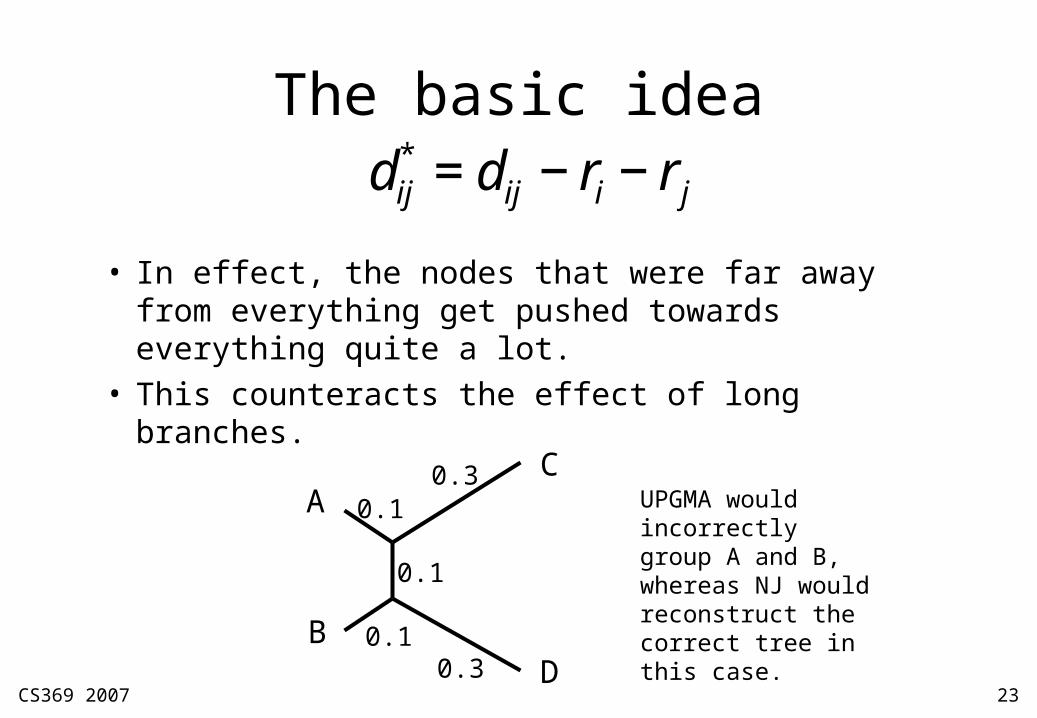
The basic idea
• We start by moving every node i closer to all other nodes by this amount:
€
ri =1n −2
dijj∑
• As a result the new (squashed) distances are:
€
dij* = dij − ri − rj
• We are pushing node i closer to all other nodes by an amount slightly more than the average distance to all other taxa.
CS369 2007 23
The basic idea
• In effect, the nodes that were far away from everything get pushed towards everything quite a lot.
• This counteracts the effect of long branches.€
dij* = dij − ri − rj
A
B
C
D
0.3
0.3
0.1
0.1
0.1
UPGMA would incorrectly group A and B, whereas NJ would reconstruct the correct tree in this case.

CS369 2007 24
Neighbor-joining
• We use an algorithm very similar to UPGMA to connect the two closest nodes, i and j, using these new squashed distances.
• We join these into a cluster and make a new node k to correspond to their ancestor, and pick distances from i, j and all other nodes to k.
• The squashed distances are updated at each step.
• See Durbin book, p171 for details.

CS369 2007 25
Runtime of the algorithm
• Both of these clustering-based algorithms take O(n3) time once we have the distance matrix.
• There are n steps and in each step we do:– (1) find the smallest distance– (2) join these two taxa– (3) compute the distance from the new ancestor to all
others• Step (1) takes O(n2) and the other two steps take
O(n)
Top Related