


Languages
Pages
Legal


Phase Behavior of Diblock Copolymer/Homopolymer Blends


Phase Behavior of Diblock Copolymer/Homopolymer Blends
By
Jiajia Zhou, M.Sc.
A Thesis
Submitted to the School of Graduate Studies
in Partial Fulfilment of the Requirements
for the Degree
Doctor of Philosophy
McMaster University
c©Copyright by Jiajia Zhou, December 2010

Doctor of Philosophy (2010) McMaster University
(Department of Physics & Astronomy) Hamilton, Ontario, Canada
TITLE: Phase Behavior of Diblock Copolymer/Homopolymer Blends
AUTHOR: Jiajia Zhou, M.Sc.
SUPERVISOR: Dr. An-Chang Shi
NUMBER OF PAGES: xiv, 120
ii

Abstract
Self-consistent field theory (SCFT) is a well established theoretical framework for
describing the thermodynamics of block copolymer melts and blends. Combined with
numerical methods, the SCFT can give useful and accurate predictions regarding the
phase behavior of polymer blends.
We have applied SCFT to study the phase behavior of blends composed of diblock
copolymers (AB) and homopolymers (C). Two cases are studied in detail. In the
first case the homopolymers have a repulsive interaction to the diblock copolymers.
We found an interesting feature in the phase diagram that there exists a bump of
the phase boundary line when A is the majority-component. In the second case,
the homopolymers have an attractive interaction to one of the blocks of the diblock
copolymers. A closed-loop of microphase separation region forms for strong interac-
tions. For both cases, we have investigated the effects of homopolymer concentration,
homopolymer chain length, and monomer-monomer interactions, on the phase behav-
ior of the system.
We also investigated micelle formation in polymer blends. Diblock copolymers (AB)
blended with homopolymers (A) can self-assemble into lamellar, cylindrical and spher-
ical micelles. The critical micelle concentrations for different geometries are deter-
mined using self-consistent field theory. The effect of varying copolymer block asym-
metry, homopolymer molecular weight and monomer-monomer interactions on micelle
morphology are examined. When the blends are confined between two flat surfaces,
the shape of the micelles may differ from that of the bulk micelles. We study the
shape variation of a spherical micelle under confinement and its dependence on the
film thickness and surface selectivity.
iii

Acknowledgements
Like life, basketball is messy and unpredictable. It has its way with you, no
matter how hard you try to control it. The trick is to experience each moment
with a clear mind and open heart. When you do that, the game –and life– will
take care of itself.
–Phil Jackson
It is hard to argue with someone as decorated as Phil Jackson, especially considering
that he has to use the toe to wear all his NBA champion rings. I like this quote because
not only it is quite wise, but also it can still make sense if you replace the basketball with
diblock copolymer.
I have had the fortune/misfortune of taking a meandering path in my graduate study,
depending on the point of view. Someone may think that it is quite a waste of time to
spend eight years in graduate school. However, as any long-distant runners can testify, the
finish time is hardly the most important criterion to evaluate a race; it is the journey, the
experience that really matter. For me, I have really enjoyed the scenic route.
I wouldn’t pass the final line (almost) without some amazing people who have helped
and cheered for me on this long journey. I want to take this opportunity to thank them.
Inevitably, I will miss some names, and for those people I apologize in advance.
I would like to thank my supervisor, Dr An-Chang Shi. You pointed me in the right
direction when I was almost lost. Thanks for giving me the opportunity to explore the
wonderful world of polymer physics (to be honest, I thought before only quantum mechanics
is the real physics). Your patience, understanding and knowledge are greatly admired and
appreciated. From you, I have learned (hopefully) how to do research and find interesting
questions. The advices you gave me, both professional and personal, have helped me a lot.
You’ve taught me so, so much –thank you.
iv

I consider myself lucky to have Dr Cecile Fradin, Dr Duncan O’Dell and Dr Maikel
Rheinstadter serve on my committee – thank you all for your advice and support throughout
my grad school. I also want to thank all my teachers at McMaster. You taught me a lot,
not just the knowledge but also how to be a good person. Special thanks to our secretaries
in the main office: Mara, Cheryl, Rosemary, Tina, Liz and Caroline. You have made my
life much easier.
The research in this thesis would not have been possible without the help of many
people. In particular, I’d like to thank all my office-mates in the softies office: Dave, Issei,
Youhai, Weihua, Jianfeng, Melissa, Ashkan and Lily. I also want to thank Dr Kari Dalnoki-
Veress and his experimental group: Adam, Marie-Josee, Jessica, Marc-Antoni, Josh and
Rob. Thanks for all the help during the years.
I want to thank all my friends at Mac, especially Laura (thanks for all those haircuts,
coffee breaks and Bridges), Jason (thanks for those smokes I bummed off you), Ning Fanlong,
Cao Jun, Chen Jun, Zhou Zhuowei, Wu Meng, Ran Wenqi, Shen Sijing, Zhao Yang, Liang
Yu and Liu Zhen. You guys are wonderful and I could not imagine what my life would be
without you. Thanks to my friends Ai Yinghua, Xiao Lingyi, Yang Lilin, Jin Xiaoliang,
Shen Wenjing, Wang Wei, Guo Yang, Zhang Rui, Qin Wenjia, Fang Hao, Zhu Taoxi, Gan
Guojun, Liu Bin and Wang Kun. Every time I run into problems, you guys are always
there for me.
I thought I’ve got almost everyone until passing afternoon starts to play in the iTunes.
Without Iron & Wine’s Our Endless Numbered Days and Beatles’ Sgt. Pepper’s Lonely
Hearts Club Band, those late nights would be much longer. So thanks. Also thanks to
Steve Jobs: the macbook I bought three years ago still works like a charm, and I probably
think buying another one if you can reduce the price further :p
Finally, I would like to thank my family: my parents Kang Zhengfen and Zhou Yiping,
my wife Su Manyu. Without your support I would never be able to make this far. Thank
you.
v

Table of Contents
Abstract iii
Acknowledgements iv
List of Figures ix
Chapter 1 Introduction 1
1.1 Diblock copolymers . . . . . . . . . . . . . . . . . . . . . . . . . . . . 1
1.2 Diblock copolymer/homopolymer blends . . . . . . . . . . . . . . . . 5
1.3 Objective and outline . . . . . . . . . . . . . . . . . . . . . . . . . . . 6
Chapter 2 Self-Consistent Field Theory 9
2.1 Notations . . . . . . . . . . . . . . . . . . . . . . . . . . . . . . . . . 10
2.2 Partition function . . . . . . . . . . . . . . . . . . . . . . . . . . . . . 11
2.3 Single-chain partition functions . . . . . . . . . . . . . . . . . . . . . 15
2.4 Canonical ensemble theory . . . . . . . . . . . . . . . . . . . . . . . . 18
2.4.1 Homogeneous Phase . . . . . . . . . . . . . . . . . . . . . . . 21
2.5 Grand canonical ensemble theory . . . . . . . . . . . . . . . . . . . . 22
2.5.1 Homogeneous Phase . . . . . . . . . . . . . . . . . . . . . . . 23
2.5.2 Activity . . . . . . . . . . . . . . . . . . . . . . . . . . . . . . 24
Chapter 3 Numerical Implementation 26
3.1 General algorithm . . . . . . . . . . . . . . . . . . . . . . . . . . . . . 27
3.1.1 General recipe . . . . . . . . . . . . . . . . . . . . . . . . . . . 29
vi

3.2 Spectral method . . . . . . . . . . . . . . . . . . . . . . . . . . . . . . 30
3.2.1 Restricted spectral method . . . . . . . . . . . . . . . . . . . . 33
3.2.2 Restricted spectral method recipe . . . . . . . . . . . . . . . . 37
3.3 Finite difference method . . . . . . . . . . . . . . . . . . . . . . . . . 38
3.3.1 Finite difference method . . . . . . . . . . . . . . . . . . . . . 39
3.3.2 The Crank-Nicolson scheme . . . . . . . . . . . . . . . . . . . 41
3.3.3 Finite difference method recipe . . . . . . . . . . . . . . . . . 41
3.3.4 ADI (Alternating-Direction Implicit) method . . . . . . . . . . 43
Chapter 4 Phase Behavior of AB/C Blends 44
4.1 Phase diagrams . . . . . . . . . . . . . . . . . . . . . . . . . . . . . . 47
4.2 Case I: fA < 0.5 . . . . . . . . . . . . . . . . . . . . . . . . . . . . . . 49
4.3 Case II: fA > 0.5 . . . . . . . . . . . . . . . . . . . . . . . . . . . . . 56
4.4 Summary . . . . . . . . . . . . . . . . . . . . . . . . . . . . . . . . . 58
Chapter 5 AB/C Blends with Attractive Interaction 60
5.1 Random phase approximation . . . . . . . . . . . . . . . . . . . . . . 62
5.2 Self-consistent field theory . . . . . . . . . . . . . . . . . . . . . . . . 71
5.3 Summary . . . . . . . . . . . . . . . . . . . . . . . . . . . . . . . . . 79
Chapter 6 Bulk micelles 81
6.1 Isolated micelles . . . . . . . . . . . . . . . . . . . . . . . . . . . . . . 83
6.2 Results and Discussions . . . . . . . . . . . . . . . . . . . . . . . . . 87
vii

6.3 Summary . . . . . . . . . . . . . . . . . . . . . . . . . . . . . . . . . 95
Chapter 7 Micelles in Thin Film 97
7.1 Hard-surface effect . . . . . . . . . . . . . . . . . . . . . . . . . . . . 99
7.2 Results and discussion . . . . . . . . . . . . . . . . . . . . . . . . . . 101
7.2.1 Geometry frustration . . . . . . . . . . . . . . . . . . . . . . . 104
7.2.2 Surface selectivity . . . . . . . . . . . . . . . . . . . . . . . . . 106
7.3 Summary . . . . . . . . . . . . . . . . . . . . . . . . . . . . . . . . . 107
Chapter 8 Summary and Perspective 109
8.1 Key results . . . . . . . . . . . . . . . . . . . . . . . . . . . . . . . . 109
8.2 Perspective . . . . . . . . . . . . . . . . . . . . . . . . . . . . . . . . 110
Bibliography 115
viii

List of Figures
1.1 Ordered structure observed in diblock copolymer melts. Gyroid (G) and
perforated-lamellar phase are adapted from ref. [9], and Fddd phase is
adapted from ref. [8]. . . . . . . . . . . . . . . . . . . . . . . . . . . . 2
1.2 (a) Theoretical phase diagram calculated using the self-consistent field
theory. (b) Experimental phase diagram measured using polystyrene-
polyisoprene diblock copolymers. Adapted from ref. [9]. . . . . . . . . 4
2.1 An illustration of the mean field approximation: an interacting many-chain
system is approximated by a single chain in an averaged potential field
ωr. . . . . . . . . . . . . . . . . . . . . . . . . . . . . . . . . . . . . . 9
2.2 The parameters used to describe the diblock copolymer/homopolymer
(AB/C) blends. . . . . . . . . . . . . . . . . . . . . . . . . . . . . . . 11
3.1 A schematic presentation of self-consistent field theory to illustrate the
relation between the density fields, the potential fields and the propa-
gators of path integral. . . . . . . . . . . . . . . . . . . . . . . . . . . 27
3.2 The spatial grid for the finite difference method. . . . . . . . . . . . . . . 40
4.1 Phase diagram of AB/C blend with parameters χABN = 11.0, χBCN =
12.0, χACN = 0 and κ = 1.0. The results are plotted in terms of the
homopolymer volume fraction φH and the A-monomer fraction of the
diblock fA. For clarity, only the largest 2-phase region is labeled. . . . 48
4.2 Phase diagram of AB/C blend with parameters χABN = 11.0, χBCN =
14.0 and χACN = 0 for three different value of κ = 0.5, 1.0 and 1.5.
The results are plotted in φH-fA axes. . . . . . . . . . . . . . . . . . . 50
ix

4.3 Spatial variables of LAM structure for AB/C blend with parameters χABN =
11.0, χBCN = 14.0, χACN = 0 and fA = 0.46. (a) Period of the LAM
structure ∆, measured in unit of Rg = Na2/6, as a function of the
homopolymer concentration φH . (b) The relative size of A-rich region
∆A, in unit of ∆, as a function of φH . . . . . . . . . . . . . . . . . . 53
4.4 C-monomer density profile for AB/C blend with parameters χABN = 11.0,
χBCN = 14.0, χACN = 0, fA = 0.46 and φH = 0.04. . . . . . . . . . 53
4.5 Phase diagram of AB/C blend with parameters χABN = 11.0, χBCN =
14.0, χACN = 0 and fA = 0.46. The results are plotted in φH-κ axes. 54
4.6 Phase diagram of AB/C blend with parameters χABN = 11.0, χACN = 0
and κ = 1.0. The results are plotted in φH-χBCN axes. . . . . . . . . 55
4.7 Phase diagram of AB/C blend with parameters χABN = 11.0, χBCN =
12.0 and χACN = 0 for three different value of κ = 0.5, 1.0 and 1.5.
The results are plotted in terms of φH and fA. . . . . . . . . . . . . 56
4.8 Phase diagram of AB/C blend with parameters χABN = 11.0, χBCN =
12.0, χACN = 0 and fA = 0.55. The results are plotted in terms of
the homopolymer volume fraction φH and the relative length of the
homopolymer κ. . . . . . . . . . . . . . . . . . . . . . . . . . . . . . . 57
4.9 Phase diagram of AB/C blend with parameters χABN = 11.0, χACN = 0
and κ = 1.0. The results are plotted in terms of the homopolymer
volume fraction φH and the interaction parameter χBCN . . . . . . . . 59
x
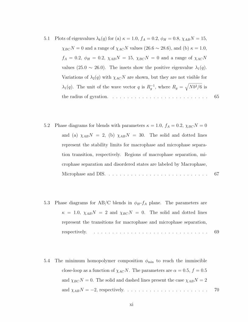
5.1 Plots of eigenvalues λk(q) for (a) κ = 1.0, fA = 0.2, φH = 0.8, χABN = 15,
χBCN = 0 and a range of χACN values (26.6 ∼ 28.6), and (b) κ = 1.0,
fA = 0.2, φH = 0.2, χABN = 15, χBCN = 0 and a range of χACN
values (25.0 ∼ 26.0). The insets show the positive eigenvalue λ1(q).
Variations of λ2(q) with χACN are shown, but they are not visible for
λ1(q). The unit of the wave vector q is R−1g , where Rg =
√Nb2/6 is
the radius of gyration. . . . . . . . . . . . . . . . . . . . . . . . . . . 65
5.2 Phase diagrams for blends with parameters κ = 1.0, fA = 0.2, χBCN = 0
and (a) χABN = 2, (b) χABN = 30. The solid and dotted lines
represent the stability limits for macrophase and microphase separa-
tion transition, respectively. Regions of macrophase separation, mi-
crophase separation and disordered states are labeled by Macrophase,
Microphase and DIS. . . . . . . . . . . . . . . . . . . . . . . . . . . . 67
5.3 Phase diagrams for AB/C blends in φH-fA plane. The parameters are
κ = 1.0, χABN = 2 and χBCN = 0. The solid and dotted lines
represent the transitions for macrophase and microphase separation,
respectively. . . . . . . . . . . . . . . . . . . . . . . . . . . . . . . . 69
5.4 The minimum homopolymer composition φmin to reach the immiscible
close-loop as a function of χACN . The parameters are α = 0.5, f = 0.5
and χBCN = 0. The solid and dashed lines present the case χABN = 2
and χABN = −2, respectively. . . . . . . . . . . . . . . . . . . . . . . 70
xi

5.5 Phase diagrams of AB/C blends with parameters κ = 1.0, χABN = 11,
χBCN = 0, and (a) χACN = −30, (b) χACN = 12. The superscripts of
HEX and BCC phase denote the components that form the cylinders
and spheres near the lattice centers. There are regions of 2-phase
coexistence between the ordered phases. . . . . . . . . . . . . . . . . 73
5.6 Phase diagram of AB/C blends with parameters κ = 1.0, χABN = 2,
χBCN = 0 and χACN = −40. The dotted line shows the RPA result. 74
5.7 Phase diagrams of AB/C blends with parameters χABN = 2, χBCN = 0,
χACN = −40 and (a) κ = 0.5, (b) κ = 1.5. . . . . . . . . . . . . . . . 77
5.8 Phase diagrams of AB/C blends with parameters κ = 1.0, χABN = 2,
χBCN = 0, and (a) χACN = −35, (b) χACN = −45. . . . . . . . . . 78
6.1 Free energy difference ∆G between a cylindrical micelle and the homoge-
neous phase, plotted as a function of copolymer chemical potential µc.
The blends have the parameters fA = 0.60, κ = 1.0 and χN = 20. . . 84
6.2 Density profiles for an isolate cylindrical micelle. The blend has the pa-
rameters fA = 0.60, κ = 1.0, χN = 20 and µc = 3.87. . . . . . . . . . 85
6.3 Dependence of µcmc on the copolymer asymmetry fA as derived from the
scaling method. Three morphologies are plotted: lamellar (blue solid
line), cylindrical (green, dashed line) and spherical (red dotted line). . 88
6.4 Dependence of µcmc on the copolymer asymmetry fA for blends with χN =
20 and κ = 1.0. The critical micelle concentrations are plotted in the
inset. Notation as in Fig. 6.3. . . . . . . . . . . . . . . . . . . . . . . 89
6.5 Dependence of µcmc and φcmc on the copolymer asymmetry fA for blends
with χN = 20 and κ = 2.0. Notation as in Fig. 6.3. . . . . . . . . . . 90
xii

6.6 Dependence of µcmc and φcmc on the copolymer asymmetry fA for blends
with χN = 50 and κ = 1.0. Notation as in Fig. 6.3. . . . . . . . . . . 90
6.7 Dependence of φcmc on the homopolymer/copolymer length ratio κ for
blends with χN = 20 and fA = 0.70. Two morphologies are plotted:
cylindrical (green, dashed line) and spherical (red dotted line). The
difference in the cmc of the two morphologies is plotted in the inset for
clarity. . . . . . . . . . . . . . . . . . . . . . . . . . . . . . . . . . . . 92
6.8 Micelle properties as a function of κ for blends with χN = 20 and fA =
0.70. The core radius (a), the corona thickness (b), the excess copoly-
mers (c) and the penetrating homopolymers (d) are plotted. Notation
as in Fig. 6.7. . . . . . . . . . . . . . . . . . . . . . . . . . . . . . . . 92
6.9 Dependence of φcmc on the interaction parameter χN for blends with κ =
1.0 and fA = 0.70. Two morphologies are plotted: cylindrical (green,
dashed line) and spherical (red dotted line). The difference in the cmc
of the two morphologies is plotted in the inset for clarity. . . . . . . . 94
6.10 Micelle properties as a function of χN for blends with κ = 1.0 and
fA = 0.70. The core radius (a), the corona thickness (b), the excess
copolymers (c) and the penetrating homopolymers (d) are plotted. No-
tation as in Fig. 6.9. . . . . . . . . . . . . . . . . . . . . . . . . . . . 94
7.1 Coordinate system for modeling the micelle formation in AB/A films. . 99
7.2 Total monomer density near the hard surface for τ = 0.15Rg. . . . . . . . 100
7.3 Monomer density profiles for a spherical micelle formed in the AB/A films.
The length unit is√Nb. . . . . . . . . . . . . . . . . . . . . . . . . . 102
xiii

7.4 Copolymer density away from the micelle (x = 4√Nb). The parameters
are the same as Fig. 7.3. . . . . . . . . . . . . . . . . . . . . . . . . . 103
7.5 (a) x- and z-radius for a spherical micelle under confinement. (b) ellipticity.
The insets in (b) are the φcB(r) profile for D = 2.0√Nb (top) and
D = 1.4√Nb (bottom). . . . . . . . . . . . . . . . . . . . . . . . . . 105
7.6 The ratio between x- and z-radius as a function of surface selectivity for
the symmetric case. The two insets show the density profile of φcB for
two different value of selectivity: Λ = 1 (left) and Λ = 50 (right). . . . 106
7.7 The density profile of φcB when the two surface have different selectivity.
(a) Λl = 0, Λu = 1; (b) Λl = 0, Λu = 50; (c) the difference. . . . . . . 107
xiv

Ph.D. Thesis ––––––––– Jiajia Zhou ––––––––– McMaster University - Physics & Astronomy ––––––––– 2010
Chapter 1
Introduction
Polymers are chain-like macromolecules in which many small molecular units,
called monomers, are linked together by covalent bonds. A macromolecule is called a
homopolymer if all of its monomers are chemically identical. Examples of homopoly-
mers are synthetic polymers like polystyrene, made of long chain of styrene. Copoly-
mers, on the other hand, contain two or more chemically distinct monomers. Most
biopolymers are copolymers: deoxyribonucleic acids (DNA) consist of long chain of
four types of nucleotides, and proteins are made up of about twenty different amino-
acids.
1.1 Diblock copolymers
Diblock copolymers are one special type of copolymers, in which the polymer
chains are composed of two blocks of different monomers [1, 2]. Physicists and
chemists are fascinated about diblock copolymers because, despite their simple chem-
ical structure, they can self-assemble into a variety of ordered structures with the
domain size in the order of nanometers. Different morphologies can be formed as
a result of a competition between the interaction energy and the chain stretching.
First of all, different blocks do not like mixing and tend to separate out into distinct
parts. One the other hand, the chemical bonds linking different blocks prevent the
separation at a macroscopic length. Therefore, diblock copolymers have to make
some comprise between the separating and mixing, resulting in the formation of var-
1

Ph.D. Thesis ––––––––– Jiajia Zhou ––––––––– McMaster University - Physics & Astronomy ––––––––– 2010
ious ordered structures. For diblock copolymers, the simplest and most common
morphologies are the so called classical structures: lamellae consisting of alternating
layers (LAM), cylinders packed on a hexagonal lattice (HEX), and spheres arranged
in a body-centered cubic lattice (BCC). There are also some complex structures: gy-
roid which is a bicontinuous phase with Ia3d symmetry [3, 4], perforated-lamellar
phase [5], and a very recently discovered Fddd phase which is a noncubic network
morphology [6, 7, 8]. Schematic pictures of these morphologies are shown in Fig. 1.1.
BCCHEXLAM
fdddPLG
Figure 1.1: Ordered structure observed in diblock copolymer melts. Gyroid (G) andperforated-lamellar phase are adapted from ref. [9], and Fddd phase is adapted fromref. [8].
Several properties of the diblock copolymer make it an ideal model system for
the study of self-assembly. First of all, in the condensed melt, the polymer chains
overlap each other and interact with many other chains. This ensures the validity of
the mean-field approximation which can greatly simplify the model. Secondly, the
high degree of polymerization allows one to model the polymers as flexible Gaussian
2

Ph.D. Thesis ––––––––– Jiajia Zhou ––––––––– McMaster University - Physics & Astronomy ––––––––– 2010
chains, whose energy is due to the stretching and has a simple form. Thirdly, the
atomic details are suppressed by the macromolecular nature of the polymers, and the
phase behavior of diblock copolymers is mainly controlled by two parameters: the
block asymmetry fA and the product of the total degree of polymerization N and
the Flory-Huggins parameter χ. Various theoretical approaches have been developed
to study the phase behavior of diblock copolymers. Among them, the self-consistent
field theory proves to be one of the most successful. Fig. 1.2 compares the phase
diagrams of diblock copolymers calculated from self-consistent field theory and from
experiments [9]. Remarkably, the theory is able to predict all the stable morphologies
and their relative positions in the phase diagram.
Edwards first introduced the idea of self-consistent field theory to polymer science.
In his 1965 paper [10], he suggested that the probability distribution of a polymer
chain may be approximated by that of a random walk in the external potential field,
and the field can be determined a posteriori from the monomer density distribution.
The theory was then applied to diblock copolymer melts by Helfand [11, 12]. Lately,
several groups have made important contributions to the theory [13, 14, 15, 16].
Early attempts to calculate the phase diagram of diblock copolymers were restricted
by limited computer resources, so approximation schemes were also developed to
further simplify the theory. Among them, the most notable ones are Leibler’s weak
segregation theory [17] and Semenov’s strong segregation theory [18]. Advances in the
modern computers and numerical methods allow one to solve the self-consistent field
theory without further approximation. The first complete phase diagram including all
the known and proposed phases of diblock copolymers was calculated by Matsen and
Schick [19] using a spectral method. Efficient algorithms to solve self-consistent field
equations in real-space have also been developed [20, 21]. Combined with numerical
methods, self-consistent field theory is capable of providing accurate predictions for
3

Ph.D. Thesis ––––––––– Jiajia Zhou ––––––––– McMaster University - Physics & Astronomy ––––––––– 2010
Figure 1.2: (a) Theoretical phase diagram calculated using the self-consistent fieldtheory. (b) Experimental phase diagram measured using polystyrene-polyisoprenediblock copolymers. Adapted from ref. [9].
4

Ph.D. Thesis ––––––––– Jiajia Zhou ––––––––– McMaster University - Physics & Astronomy ––––––––– 2010
the phase behavior of polymeric systems. A number of monographs [1, 22] and review
articles [9, 23, 24, 25] on self-consistent field theory are available in the literature.
It can be concluded that self-consistent field theory provides a powerful theoretical
framework to study block copolymers.
1.2 Diblock copolymer/homopolymer blends
Blending provides an effective and economical route to obtain new materials be-
cause the end products can have combinative and enhanced properties of their con-
stituents. In general, different homopolymers do not mix due to the unfavorable
thermodynamics. The entropy of mixing is often insignificant for long-chain ho-
mopolymers. Copolymers are ideal candidates to use as compatibilizers, which are
utilized to increase the miscibility of polymers. From a theoretical point of view,
the mix of homopolymers with diblock copolymers provides new behavior. Therefore
a better understanding of the phase behavior of diblock copolymer/homopolymer
blends is highly desirable.
There are two different angles we can take to approach this system. One is to treat
the diblock copolymers as the majority component and we slowly add in homopoly-
mers. The key question here is how the homopolymers distribute in the copolymer
matrix. In general, the homopolymers can either separate from the diblock copoly-
mers, or localize in domains of like blocks. In the former case, macrophase separation
occurs, while in the latter situation, the blends may undergo order-order transitions.
Using the ordered structure formed by the diblock copolymer as a template, the
homopolymers can be located in the regions where the copolymer chains are strongly
stretched and thus relieve the packing frustration. In turn, new structures which are
not found in diblock copolymer melts may be stabilized, among them are the double
5

Ph.D. Thesis ––––––––– Jiajia Zhou ––––––––– McMaster University - Physics & Astronomy ––––––––– 2010
diamond phase with a Pn3m symmetry [26] and the plumber’s nightmare phase with
an Im3m symmetry [27].
From the other end of the spectrum, when a small amount of diblock copolymers
are added into a homopolymer melt, local aggregates called micelles can be formed.
Normally, one block of the copolymers is miscible to the homopolymers and the other
one not. The local self-assembly is driven by this unbalance of miscibility. Specif-
ically, the miscible blocks stay on the surface of the micelles, while the immiscible
blocks are buried in the interior. The process of micelle formation is similar to the
segregation of surfactants in water and the formation of bilayers from lipids. De-
pending on the copolymer configuration and interaction parameters, micelles with
different shapes can be formed; they can be flat bilayer sheets, cylinders or spheres.
A quantitative understanding of how the micelle shapes are determined by various
factors is important from the fundamental polymer physics point of view.
Beside providing a paradigm to study self-assembly, block copolymer micelles can
also be used for several applications. Various types of micelle shape can be used as
templates for the fabrication of nano-structured materials. Also, diblock micelles are
significantly more stable than the ones by surfactants of low-molecular weight. This
offers opportunities to utilize spherical micelles for drug delivery.
Because of its success in diblock copolymer melts, self-consistent field theory is
a natural choice to study the phase behavior of diblock copolymer/homopolymer
blends.
1.3 Objective and outline
Using self-consistent field theory as the main tool, we address several problems
related to the phase behavior of diblock copolymer/homopolymer blends in this thesis.
6

Ph.D. Thesis ––––––––– Jiajia Zhou ––––––––– McMaster University - Physics & Astronomy ––––––––– 2010
Chapter 2 reviews the theoretical framework of self-consistent field theory, using
the AB/C blend as an example. The theory is developed in both canonical and grand
canonical ensembles. Chapter 3 presents the numerical implementation of the theory.
The central problem is how to solve a modified diffusion equation. Two methods,
the spectral method and the finite difference method, are discussed in detail. The
purpose of these two chapters is to lay the foundation for later applications.
In Chapter 4 and 5, we apply self-consistent field theory to study the phase be-
havior of AB/C blends. Chapter 4 considers blends of asymmetric copolymers. The
addition of the homopolymer C provides further control of the phase diagram and en-
riches the phase behavior. We examine the effect of the homopolymer concentration,
the homopolymer chain length, and the monomer-monomer interactions. In partic-
ular, an interesting feature of the phase diagram, a bump of the phase boundary
line when A is the minority component, is discussed in term of competition between
entropy and energy effects.
New phase behavior emerges when the interaction between the homopolymer C
and one of the blocks becomes attractive. Inspired by recently experimental work
of Chen et al. [28], we study the AB/C blends where all three binary pairs, A/B,
B/C and C/A, are miscible. Despite the miscibility of the binary pairs, a closed-loop
immiscible region exists when the A/C and B/C pair interactions are sufficiently dif-
ferent. Inside the closed-loop, the system undergoes microphase separation, exhibiting
different ordered structures. In Chapter 5, we use both random phase approximation
and self-consistent field theory to interrogate this interesting phenomenon.
We present the study of micellar structure of AB/A blends in Chapter 6 and 7.
The subject of Chapter 6 is the micelle shape transition in bulk. Diblock copoly-
mers added into homopolymer melts can self-assemble into lamellar, cylindrical and
spherical micelles. The critical micelle concentrations for different geometries are de-
7

Ph.D. Thesis ––––––––– Jiajia Zhou ––––––––– McMaster University - Physics & Astronomy ––––––––– 2010
termined using self-consistent field theory. The effects of varying copolymer block
asymmetry, homopolymer molecular weight and monomer-monomer interaction on
micelle morphology are investigated.
In Chapter 7, we consider micelle formation under planar confinement. The shape
of the micelles under confinement may differ from the bulk micelles due to the pres-
ence of two impenetrable surfaces. We use a real-space self-consistent field theory to
examine the properties of an isolated micelle. We focus on the effect of film thickness
and surface selectivity on the micelles. The results reveal that the spherical symme-
try is broken by the film geometry, whereas the top-down symmetry is broken by the
surface selectivity.
In Chapter 8 we summarize the key results of this thesis and give some perspective
on future directions in this research area.
8

Ph.D. Thesis ––––––––– Jiajia Zhou ––––––––– McMaster University - Physics & Astronomy ––––––––– 2010
Chapter 2
Self-Consistent Field Theory
The system of interest consists of many polymer chains interacting with each
other. In the framework of self-consistent field theory, this essentially many-body
problem is replaced by the problem of an ideal Gaussian chain in an effective mean-
field potential. This procedure is shown schematically in Fig. 2.1. If the mean-field
potential can be specified, the thermodynamical properties of the system, such as
the partition function and monomer densities, can be expressed in terms of the chain
propagators, which are related to the mean field by the modified diffusion equations.
From the monomer densities, a new mean-field potential can be constructed. The
procedure results in a closed set of equations that can be solved self-consistently using
numerical methods. Once the self-consistent solutions are reached, the free energy
can be evaluated for various ordered structures. A phase diagram is constructed by
finding the morphology with the lowest free energy.
Figure 2.1: An illustration of the mean field approximation: an interacting many-chain system is approximated by a single chain in an averaged potential field ωr.
9

Ph.D. Thesis ––––––––– Jiajia Zhou ––––––––– McMaster University - Physics & Astronomy ––––––––– 2010
In this chapter, we develop the self-consistent field theory for a binary blend of AB
diblock copolymers and C homopolymers. We formulate the theory using a canonical
ensemble approach first. Then the theory will be extended to the grand canonical
ensemble.
2.1 Notations
In this section, we introduce the parameters and variables to describe the binary
blends of diblock copolymer AB and homopolymer C. We will try to keep the notation
consistent throughout this thesis.
The diblock copolymer AB and homopolymer C are labeled as polymer 1 and 2,
respectively. In the canonical ensemble, the volume, the temperature and the numbers
of polymer chains are the controlling thermodynamic parameters. We consider n1
diblock copolymer and n2 homopolymer chains in a volume V . Each polymer chain
is composed of Np monomers of species α = A,B for p = 1 or α = C for p = 2.
The chain length of the diblock copolymer is N1 = κ1N . We choose N1 = N to be
the reference chain length, so κ1 = 1. The homopolymer has a length of N2 = κ2N .
The ratio of the two polymer lengths is κ = N2/N1 = κ2. For the diblock copolymer,
the degrees of polymerization of the different blocks are NA = fAN and NB = fBN
(where fA + fB = 1). For the homopolymer, we have NC = N2 = κN .
Each type of monomer is associated with a statistical length bα = σαb, where
b is a reference length. The monomers are assumed to have the same monomer
density ρ0. The blend is incompressible, mimicking the hardcore monomer-monomer
interaction, and the hardcore volume per monomer is ρ−10 . The volume fractions (or
concentrations) for the copolymers and homopolymers are 1−φH and φH , respectively.
We will use the convention that all lengths are scaled by the radius of gyration for the
10

Ph.D. Thesis ––––––––– Jiajia Zhou ––––––––– McMaster University - Physics & Astronomy ––––––––– 2010
NA = fAN NB = fBN
NC = !N
!AB
!AC !BC
Parameter space:
!H
1− !H
(!, fA, "H , #ABN, #BCN, #ACN)
Diblock copolymer AB
Homopolymer C
Figure 2.2: The parameters used to describe the diblock copolymer/homopolymer(AB/C) blends.
copolymer, Rg = b√N/6. The chain length is scaled by the copolymer chain length
N . Finally, the interactions between each pair are characterized by the Flory-Huggins
parameters: χAB, χBC and χAC . All relevant parameters are summarized in Fig. 2.2.
2.2 Partition function
Polymer chains with high degree of polymerization can be effectively treated as
continuous, linearly elastic filaments without bending penalty. This is the so called
continuous Gaussian chain model [29]. In this model, the conformation of an α-
block of the i-th chain is denoted by a continuous-space curve Rαi (s), with s being
the variable analog to the arc length, varying from 0 to Nα. For a given chain
conformation Rαi (s), the local concentration of α-monomers at position r is,
φα(r) =1
ρ0
np∑i=1
∫ Nα
0dsδ(r−Rα
i (s)). (2.1)
11

Ph.D. Thesis ––––––––– Jiajia Zhou ––––––––– McMaster University - Physics & Astronomy ––––––––– 2010
This is a set of delta functions located at the position of each chain segment. Ev-
idently, this microscopic density function is a very singular function of the chain
position. The hat on the variable φα emphasizes the dependence on the chain con-
formation.
The potential energy of a continuous Gaussian chain can be written as
U0[Rαi (s)] =
3kBT
2b2α
∫ Nα
0ds
∣∣∣∣∣dRαi (s)
ds
∣∣∣∣∣2
, (2.2)
where dRαi (s)/ds is the derivative of the curve Rα
i (s) at contour position s. We use
the square bracket notation U0[Rαi (s)] to indicate that U0 is a functional of Rα
i (s).
If we view the space curve as a flexible rubber band, |dRαi (s)/ds| corresponds to
the local stretching at the contour position s, then eqn (2.2) is a summation of
a harmonic potential energy contribution from each segment ds, with the spring
constant being 3kBT/2b2α. Potential energy of this form is commonly known as the
Edwards Hamiltonian.
The probability distribution of observing Rαi (s) in the configuration space is the
standard Boltzmann distribution
p0[Rαi (s)] = A exp
− 3
2b2α
∫ Nα
0ds
(dRα
i (s)
ds
)2 , (2.3)
where A is a normalization constant. The probability P0[Ri(s)] for a given chain
conformation Ri(s) is then given by
P0[Ri(s)] =n1∏i=1
p0(RA
i (s))p0(RBi (s))δ[RA
i (NA)−RBi (NB)]
n2∏i=1
p0(RC
i (s)),
(2.4)
where the connection between the A- and B-block from the same chain is ensured by
the delta functions.
12

Ph.D. Thesis ––––––––– Jiajia Zhou ––––––––– McMaster University - Physics & Astronomy ––––––––– 2010
The partition function of the blend can be written in terms of the functional
integral over all the chain conformations,
Z =zn1
01 zn202
n1!n2!
∫DRi(s)P0[Ri(s)]
∏r
δ(∑α
φα(r)− 1)e−W [φ(r)], (2.5)
where z0p is the kinetic energy contribution to the partition functions, and n1!n2! in
the denominator counts for the fact that chains of the same type are indistinguish-
able. The delta-functions are introduced to enforce the incompressibility condition.
The exponent term in the partition function is the Boltzmann factor associated with
the monomer-monomer interaction potential W [φ(r)], which is a functional of the
microscopic densities φ(r). We use the simple Flory-Huggins form of interaction
energy
W [φ(r)] = ρ0
∫dr[χABφA(r)φB(r) + χBC φB(r)φC(r) + χAC φA(r)φC(r)
]=
1
2
∑α 6=β
ρ0χαβ
∫drφα(r)φβ(r). (2.6)
The partition function Z contains all the information about the thermodynamics
of the AB/C system. However the evaluation of Z is not possible since the integrand
depends on the chain conformation through the microscopic density functions φα.
A standard algebraic trick is to use the identity
1 =∫
Dφα∏α
∏r
δ(φα(r)− φα(r)), (2.7)
where φα(r) is a dummy function for the functional integration and will later be
identified as the average monomer density. Inserting this identity into expression
(2.5), we have
Z =zn1
01 zn202
n1!n2!
∫Dφα(r)
∏r
δ(∑α
φα(r)− 1)e−W [φ(r)]
×∫
DRi(s)P0[Ri(s)]∏α
∏r
δ(φα(r)− φα(r)). (2.8)
13

Ph.D. Thesis ––––––––– Jiajia Zhou ––––––––– McMaster University - Physics & Astronomy ––––––––– 2010
Furthermore, auxiliary fields can be introduced by using the integral definition of
the delta function:
1 =∫
Dφα(r)Dωα(r) exp
[∑α
ρ0
∫drωα(r)(φα(r)− φα(r))
]. (2.9)
The range of the ωα(r) integral is along a line in the complex plane from −i∞ to i∞.
The field ωα(r) can be viewed as a chemical potential field that is thermodynamically
conjugate to the density field φα(r) [30]. Substituting the identity (2.9) into the
partition function expression (2.8), we have
Z =zn1
01 zn202
n1!n2!
∫Dφα(r)Dωα(r)
∏r
δ(∑α
φα(r)− 1)
× exp
[∑α
ρ0
∫drωα(r)φα(r)−W [φ]
]
×∫
DRi(s)P0[Ri(s)] exp
[−∑α
ρ0
∫drωα(r)φα(r)
]. (2.10)
The advantage of this form is that the integration over the chain conformation
is done with the relatively simple integrand exp[−∑α ρ0
∫drωα(r)φα(r)]. With the
Gaussian probability distributions (2.3) and the definition of the microscopic density
(2.1), the integral over the chain conformation can be written as,
∫DRi(s)P0[Ri(s)] exp
[−∑α
ρ0
∫drωα(r)φα(r)
]
=n1∏i=1
∫DRA
i (s)DRBi (s)p0[RA
i (s)]p0[RBi (s)]
×δ[RAi (NA)−RB
i (NB)] exp
− ∑α=A,B
∫ Nα
0dsωα(Rα
i (s))
×n2∏i=1
∫DRC
i (s)p0[RCi (s)] exp
[−∫ NC
0dsωC(Rα
i (s))
]= (Q1V )n1(Q2V )n2 , (2.11)
14

Ph.D. Thesis ––––––––– Jiajia Zhou ––––––––– McMaster University - Physics & Astronomy ––––––––– 2010
where Qp is the partition function of a polymer chain of type p in the external field
ωα (α = A,B for p = 1 and α = C for p = 2). These single-chain partition functions
are defined by
Q1 =1
V
∫DRA
i (s)DRBi (s)p0[RA
i (s)]p0[RBi (s)]
×δ[RAi (NA)−RB
i (NB)] exp
− ∑α=A,B
∫ Nα
0dsωα(Rα
i (s))
(2.12)
Q2 =1
V
∫DRC
i (s)p0[RCi (s)] exp
[−∫ NC
0dsωC(RC
i (s))
]. (2.13)
Furthermore, the incompressibility condition can be enforced using a Lagrange
multiplier field η(r),
δ(∑α
φα(r)− 1) = exp
[−ρ0
∫drη(r)(
∑α
φα(r)− 1)
]. (2.14)
With the definition of the single-chain partition function Qp and the field η(r),
the partition function of the AB/C blend can be rewritten as a functional integral
over three fields: the density fields φα(r), the chemical potential fields ωα(r), and the
Lagrange multiplier field η(r),
Z =∫
Dφα(r)Dωα(r)Dη(r)∏r
exp
[∑α
ρ0
∫drωα(r)φα(r)−W [φ]
−ρ0
∫drη(r)(
∑α
φα(r)− 1)
](z01Q1V )n1
n1!
(z02Q2V )n2
n2!. (2.15)
The dependence of the chain conformation has been absorbed into the single-chain
partition functions Qp. This formulation of the partition function is the starting point
of our theory.
2.3 Single-chain partition functions
The quantity Qp[ωα] in the above expression is the partition function for a single
chain subjected to the external field ωα(r). It is a functional of the field ωα(r), and
15

Ph.D. Thesis ––––––––– Jiajia Zhou ––––––––– McMaster University - Physics & Astronomy ––––––––– 2010
contains the chain conformation contribution to the total partition function Z. In
the following, we discuss the partition function for the diblock copolymer AB and
homopolymer C using the path integral formula [31].
The single-chain partition function Q1 for AB diblock copolymer can be expressed
in terms of the chain propagators Qα(r, s|r′),
Q1 =1
V
∫dr1dr2dr3QA(r1, NA|r2)QB(r2, NB|r3), (2.16)
where the chain propagators are defined by
Qα(r, s|r′) =∫ R(s)=r
R(0)=r′DR(s) exp
− ∫ s
0ds′
3
2b2α
[dR(s′)
ds′
]2
+ ωα(R(s′))
.(2.17)
The physical meaning of these propagators is that Qα(r, s|r′) represents the condi-
tional probability of monomer s at position r, given the monomer 0 is at position r′,
in the presence of an external field ωα(r).
From the definition (2.17), we can easily check the relation
Qα(r, s|r′) =∫
dr′′Qα(r, s− s′′|r′′)Qα(r′′, s′′|r′). (2.18)
This relation is based on the fact the propagator for a sub-chain [0, s] is independent
of the position of s′′-monomer (0 < s′′ < s). Equation of the form (2.18) is referred
to as a Chapman-Kolmogorov equation in the theory of stochastic process [32].
The integral form of the Chapman-Kolmogorov equation is difficult to use and
sometimes a differential form is preferred. The corresponding differential equation is
known as the Fokker-Planck equation in probability theory [32] and the Feynman-Kac
formula in quantum mechanics [33]:
∂
∂sQα(r, s|r′) =
b2α
6∇2Qα(r, s|r′)− ωα(r)Qα(r, s|r′). (2.19)
The initial conditions is Qα(r, 0|r′) = δ(r − r′). This equation is commonly referred
to as a modified diffusion equation in the polymer literature.
16

Ph.D. Thesis ––––––––– Jiajia Zhou ––––––––– McMaster University - Physics & Astronomy ––––––––– 2010
In later applications, it is convenient to use the end-integrated propagators, defined
by integrating the end position r′ of function Qα(r, s|r′)
qα(r, s) =∫
dr′Qα(r, s|r′), (2.20)
q+α (r, s) =
∫dr′dr′′Qα(r, s|r′)Qβ(r′, Nβ|r′′), (2.21)
where β = B if α = A and vice versa. These end-integrated propagators satisfy the
same differential equation as Qα(r, s|r′), but with different initial conditions
qα(r, 0) = 1, (2.22)
q+α (r, 0) =
∫dr′Qβ(r, Nβ|r′) = qβ(r, Nβ). (2.23)
Using the end-integrated propagators, the single-chain partition function Q1 can be
expressed as
Q1 =1
V
∫drqA(r, NA) =
1
V
∫drqB(r, NB). (2.24)
The single-chain partition function Q2 for C homopolymer can also be expressed
in terms of the chain propagators QC(r, s|r′),
Q2 =1
V
∫dr1dr2QC(r1, NC |r2) (2.25)
where the definition of the chain propagator QC(r, s|r′) is the same as QA(r, s|r′) and
QB(r, s|r′). It also satisfies the same modified diffusion equation (2.19) with the same
initial condition.
The end-integrated propagator qC(r, s) can also be defined as,
qc(r, s) =∫
dr′QC(r, s|r′). (2.26)
Comparing to the diblock copolymer, one end-integrated propagator is sufficient for
homopolymers.
17

Ph.D. Thesis ––––––––– Jiajia Zhou ––––––––– McMaster University - Physics & Astronomy ––––––––– 2010
The single-chain partition function for the homopolymer is written in terms of the
propagator,
Q2 =1
V
∫drqC(r, NC). (2.27)
2.4 Canonical ensemble theory
In canonical ensemble, the number of polymer chains is fixed. We can write the
partition function in terms of an “effective Hamiltonian” [22, 34],
Z =∫
DφαDωα∏r
δ(∑α
φα(r)− 1) exp
[∑α
ρ0
∫drωα(r)φα(r)−W [φα]
]
×(z01Q1V )n1
n1!
(z02Q2V )n2
n2!
=∫
DφαDωα∏r
δ(∑α
φα(r)− 1) exp[−H[φα, ωα]
], (2.28)
where the effective Hamiltonian is given by
H[φα, ωα] = W [φα]−∑α
ρ0
∫drωα(r)φα(r)− ln
(z01Q1V )n1
n1!− ln
(z02Q2V )n2
n2!
=1
2
∑α 6=β
ρ0χαβ
∫drφα(r)φβ(r)−
∑α
ρ0
∫drωα(r)φα(r)
−∑p
np lnz0peQpV
np, (2.29)
where the Stirling formula n! ≈ (n/e)n is used.
We make some simple manipulations to the eqn (2.29). They are (i) using the
average concentrations φp = npNp/ρ0V , (ii) using the radius of gyration Rg = b√N/6
as the length scale, (iii) redefining the fields by including the factor N , Nωα(r) →
ωα(r). After these manipulations, we arrive at the result,
H[φα, ωα] =ρ0R
3g
N
1
2
∑α 6=β
χαβN∫
drφα(r)φβ(r)−∑α
∫drωα(r)φα(r)
−V∑p
φpκp
lnz0peNpQp
ρ0φp
. (2.30)
18

Ph.D. Thesis ––––––––– Jiajia Zhou ––––––––– McMaster University - Physics & Astronomy ––––––––– 2010
We can also write this in terms of an effective Hamiltonian density,
h[φα, ωα] ≡NH[φα, ωα]
ρ0R3gV
=1
V
∫dr
1
2
∑α 6=β
χαβNφα(r)φβ(r)−∑α
ωα(r)φα(r)
−∑p
φpκp
lnQp +∑p
φpκp
ln(φpe
) +∑p
µ0pφp, (2.31)
where µ0p ≡ (N/Np) ln(ρ0/z0pNp) are constants which can be neglected.
Following the same procedure, the modified diffusion equation for the propagators
can be rewritten in the form,
∂
∂sqα(r, s) = σ2
α∇2qα(r, s)− ωα(r)qα(r, s). (2.32)
The equations for q+α (r, s) (α = A,B) and qC(r, s) have the same form. The initial
conditions are
qα(r, 0) = 1, (2.33)
q+α (r, 0) = qβ(r, fβ), (2.34)
qC(r, 0) = 1. (2.35)
In terms of the propagators, the single-chain partition functions are given by
Q1 =1
V
∫drq+
A(r, fA) =1
V
∫drq+
B(r, fB), (2.36)
Q2 =1
V
∫drqC(r, κ2). (2.37)
The partition function of the system is then written in the form,
Z =∫
DφαDωαDη exp[− Ω[φα, ωα, η]
], (2.38)
Ω[φα, ωα, η] = H[φα, ωα] + ρ0R3g
∫drη(r)(
∑α
φα(r)− 1). (2.39)
19

Ph.D. Thesis ––––––––– Jiajia Zhou ––––––––– McMaster University - Physics & Astronomy ––––––––– 2010
At this point, no approximation has been made except the minor one of Stirling’s
formula. The thermodynamic properties of a blend AB/C is completely determined
if we can evaluate the functional integral (2.38). Unfortunately, except for some very
special cases, the integral cannot be carried out exactly. Therefore, we need approxi-
mate methods to proceed. The most fruitful method is the mean field approximation,
which amounts to replacing the functional integral (2.38) by the value of the integrand
at its saddle point. Therefore, this approximation is also referred as saddle-point ap-
proximation or steepest descent method. Technically the approximation is obtained
by demanding that the functional derivatives of Ω[φα, ωα, η] with respect to
the fields are zero,
δΩ[φα, ωα, η]δωα(r)
= 0, (2.40)
δΩ[φα, ωα, η]δφα(r)
= 0, (2.41)
δΩ[φα, ωα, η]δη(r)
= 0, (2.42)
which leads to the following mean-field equations,
φα(r) = 〈φα(r)〉 (2.43)
ωα(r) =∑β 6=α
χαβN [φβ(r)− φβ(r)] + η(r), (2.44)
∑α=A,B,C
φα(r) = 1. (2.45)
Eqn (2.43) confirms that φα(r) is equal to 〈φα(r)〉, the thermal average of the
microscopic density in a system of non-interacting chains subjected to the external
fields ωα(r). The dependence on the external fields are through the propagators
φα(r) =φ1
Q1
∫ fα
0dsqα(r, s)q+
α (r, fα − s) α = A,B, (2.46)
φC(r) =φ2
κ2Q2
∫ κ2
0dsqC(r, s)qC(r, κ2 − s). (2.47)
20

Ph.D. Thesis ––––––––– Jiajia Zhou ––––––––– McMaster University - Physics & Astronomy ––––––––– 2010
Eqn (2.44) relates the mean-field potential to the average monomer density. We
also add some constants to the fields to make∫
drωα(r) = 0. Those constants are
φA = φ1fA, φB = φ1fB, φC = φ2. (2.48)
Eqn (2.45) is simply the incompressible condition.
Within the mean-field approximation, the Helmholtz free energy density is ob-
tained by inserting the mean field solution into expression (2.31),
fMF =1
V
∫dr
1
2
∑α 6=β
χαβNφα(r)φβ(r)−∑α
ωα(r)φα(r)
−∑p
φpκp
lnQp +∑p
φpκp
ln(φpe
) +∑p
µ0pφp. (2.49)
2.4.1 Homogeneous Phase
The simplest solution of the mean-field equations is obtained for a homogeneous
phase, in which the monomer densities and the mean-field potentials are constant,
φα(r) = φα and ωα(r) = 0, leading to the trivial solution qα(r, s) = q+α (r, s) = 1. The
free energy density of a homogeneous phase is therefore given by
fH = χABNfAfBφ21 +(χACNfA+χBCNfB)φ1φ2 +
φ1
κ1
lnφ1
e+φ2
κ2
lnφ2
e+µ01φ1 +µ02φ2.
(2.50)
It is noticed that this free energy has the standard Flory-Huggins form [35].
21

Ph.D. Thesis ––––––––– Jiajia Zhou ––––––––– McMaster University - Physics & Astronomy ––––––––– 2010
2.5 Grand canonical ensemble theory
In the grand canonical ensemble, the numbers of polymer chains vary to maintain
chemical equilibrium. The controlling parameters are the chemical potentials µ1 and
µ2. The grand partition function is defined by,
ς =∞∑
n1=0
∞∑n2=0
en1µ1+n2µ2Zn1,n2
=∫
DφαDωα∏r
δ(∑α
φα(r)− 1) exp
[∑α
ρ0
N
∫drωα(r)φα(r)−W [φα]
]
×∞∑
n1=0
(z01Q1V )n1
n1!
∞∑n2=0
(z02Q2V )n2
n2!
=∫
DφαDωα∏r
δ(∑α
φα(r)− 1) exp[−HG[φα, ωα]
], (2.51)
where HG is given by,
HG[φα, ωα] =1
2
∑α 6=β
ρ0χαβ
∫drφα(r)φβ(r)−
∑α
ρ0
N
∫drωα(r)φα(r)
−eµ1z01Q1V − eµ2z02Q2V. (2.52)
The corresponding energy density is
hG[φ, ω] ≡ N
ρR3gV
HG(φ, ω)
=1
V
∫dr
1
2
∑α 6=β
χαβNφα(r)φβ(r)−∑α
ωα(r)φα(r)
−eµ1−µ01Q1 − eµ2−κ2µ02
Q2
κ2
, (2.53)
where µ0p ≡ (1/κp) ln(ρ0/z0pNp) are constants defined before for the canonical en-
semble.
The partition function of the system is then written in the form,
ς =∫
DφαDωαDη exp[− Ω[φα, ωα, η]
], (2.54)
Ω[φα, ωα, η] = HG[φα, ωα] + ρ0R3g
∫drη(r)(
∑α
φα(r)− 1). (2.55)
22

Ph.D. Thesis ––––––––– Jiajia Zhou ––––––––– McMaster University - Physics & Astronomy ––––––––– 2010
The mean-field equations are again derived by demanding the functional deriva-
tives of Ω to vanish, which leads to the following mean-field equations,
φα(r) = e∆µ1
∫ fα
0dsqα(r, s)q+
α (r, fα − s) α = A,B, (2.56)
φC(r) =eκ2∆µ2
κ2
∫ κ2
0dsqC(r, s)q+
C (r, κ2 − s), (2.57)
ωα(r) =∑β 6=α
χαβNφβ(r) + η(r), (2.58)
∑α=A,B,C
φα(r) = 1. (2.59)
The control parameter ∆µp = µp − µ0p = µp/κp − µ0p, is the effective chemical
potential per monomer.
Once solutions of the mean-field equations are obtained, the Gibbs free energy
density can be computed using the expression,
gMF =1
V
∫dr
1
2
∑α 6=β
χαβNφα(r)φβ(r)−∑α
ωα(r)φα(r)
− e∆µ1Q1 − eκ2∆µ2Q2
κ2
.
(2.60)
2.5.1 Homogeneous Phase
For a disordered phase all the concentrations and fields are constants. The prop-
agators are easily to obtain in this case,
Qα(r, s|r′) = e−ωαsδ(r− r′), (2.61)
qα(r, s) = e−ωαs, α = A,B,C, (2.62)
q+α (r, s) = e−ωαs−ωβfβ , α, β = A,B, (2.63)
Q1 = e−ωAfA−ωBfB , (2.64)
Q2 = e−ωCκ2 . (2.65)
Therefore the mean-field equations become,
φA = e∆µ1Q1fA = φ1fA, (2.66)
23

Ph.D. Thesis ––––––––– Jiajia Zhou ––––––––– McMaster University - Physics & Astronomy ––––––––– 2010
φB = e∆µ1Q1fB = φ1fB, (2.67)
φC = eκ2∆µ2Q2 = φ2, (2.68)
φ1 = e∆µ1−ωAfA−ωBfB , (2.69)
φ2 = eκ2(∆µ2−ωC), (2.70)
ωα =∑β 6=α
χαβNφβ + η, (2.71)
∑α
φα =∑p
φp = 1. (2.72)
The Gibbs free energy density is,
gH =1
2
∑α 6=β
χαβNφαφβ −∑α
ωαφα − e∆µ1Q1 − eκ2∆µ2Q2
κ2
. (2.73)
2.5.2 Activity
It is useful to note that the densities φα(r) and the free energy are invariant under
the transformation,
∆µp → ∆µp + µ0 ωα = ωα + µ0. (2.74)
This is easy to understand because it is the energy difference matters rather than the
absolute value of the energy. The partition function changes as Qp → e−κpµ0Qp, but
the combination eκp∆µpQp is invariant under the transformation (2.74).
Using this property, we can choose µ0 = −∆µ1 to set the factor e∆µ1 to 1. The
mean-field equations become,
φA(r) =∫ fA
0ds qA(r, s)q+
A(r, fA − s) (2.75)
φB(r) =∫ fB
0ds qB(r, s)q+
B(r, fB − s) (2.76)
φC(r) = z∫ κ2
0ds qC(r, s)qC(r, κ2 − s), (2.77)
ωα(r) =∑β 6=α
χαβNφβ(r) + η(r), (2.78)
24
Ph.D. Thesis ––––––––– Jiajia Zhou ––––––––– McMaster University - Physics & Astronomy ––––––––– 2010
∑α=A,B,C
φα(r) = 1, (2.79)
where z = exp(κ2(∆µ2 −∆µ1))/κ2.
The Gibbs free energy density can be computed using the expression,
gMF =1
V
∫dr
1
2
∑α 6=β
χαβNφα(r)φβ(r)−∑α
ωα(r)φα(r)
−Q1 − zQ2. (2.80)
This free energy is often used as the starting point for the calculation in grand
canonical ensemble.
25

Ph.D. Thesis ––––––––– Jiajia Zhou ––––––––– McMaster University - Physics & Astronomy ––––––––– 2010
Chapter 3
Numerical Implementation
The mean-field approximation employed in the self-consistent field theory simpli-
fies the model considerably, but solutions to the mean-field equations are still difficult
to obtain due to the nonlinear and non-local nature of the equations. Further ap-
proximations exist to derive an analytic expression for the partition function and the
chain propagators. Noticeable examples are Leibler’s weak segregation theory [17]
and Semenov’s strong segregation theory [18]. These analytic methods are useful to
gain some insights on the system behavior at extreme conditions, but a more gener-
alized method that can be applied to any segregation is desirable. For this purpose,
a variety of numerical methods have been developed for the self-consistent field the-
ory. They are powerful tools and capable of giving accurate predictions regarding the
complex phase behavior of polymer mixtures.
In this chapter, we discuss the numerical methods used in this thesis. Using
the example of AB/C blends, we present the details of procedure to compute the
equilibrium structures and phase diagrams of polymer mixtures. In Section 3.1, we
present the general procedure to solve the mean-field equations, using an iteration
method. Two classes of numerical methods are discussed in detail: the spectral
method (Section 3.2) and the finite difference method (Section 3.3). The spectral
method is used to calculate the phase diagrams for the AB/C blends, while the finite
difference method is employed in the study of micellization in AB/A blends.
26

Ph.D. Thesis ––––––––– Jiajia Zhou ––––––––– McMaster University - Physics & Astronomy ––––––––– 2010
3.1 General algorithm
In order to calculate the equilibrium structures of AB/C blends using self-consistent
field theory, we have to solve for two sets of unknown fields: the monomer density
fields φα(r) and the chemical potential fields ωα(r). These two fields are closely
related and one can be determined with the knowledge of the other one. Therefore,
they should be determined in such a way that they do not contradict each other, i.e.,
the self-consistent condition. In Fig. 3.1 , we show the relation between the density
and potential fields.
!!(r)monomer density fields
chemical potential fields !!(r)
q!(r, s)propagatorseqn. (3.1)
eqn. (3.2)
eqn. (3.3)-(3.7)
Figure 3.1: A schematic presentation of self-consistent field theory to illustrate therelation between the density fields, the potential fields and the propagators of pathintegral.
From density fields to potential fields: ωα = F (φα)
The potential fields can be evaluated from the densities using
ωα(r) =∑β 6=α
χαβN [φβ(r)− φβ] + η(r). (3.1)
27

Ph.D. Thesis ––––––––– Jiajia Zhou ––––––––– McMaster University - Physics & Astronomy ––––––––– 2010
The potential fields include the Flory-Huggins interactions and an Lagrange multiplier
field η(r) to ensure the incompressibility.
From potential fields to density fields: φα = G (ωα)
When the potential fields are known, the densities can be calculated through
the end-integrated propagators. For the diblock copolymer AB, the end-integrated
propagators qα(r, s) and q+α (r, s) (α = A,B) are solutions of the modified diffusion
equations in the mean field ωα(r),
∂
∂sqα(r, s) = σ2
α∇2qα(r, s)− ωα(r)qα(r, s), (3.2)
with the initial condition qα(r, 0) = 1, q+α (r, 0) = qβ(r, fβ). For the homopolymer
C, one end-integrated propagator qC(r, s) is sufficient. It satisfies the same diffusion
equation with initial condition qC(r, 0) = 1.
The density fields then can be calculated from
φA(r) =φ1
Q1
∫ fA
0dsqA(r, s)q+
A(r, fA − s), (3.3)
φB(r) =φ1
Q1
∫ fB
0dsqB(r, s)q+
B(r, fB − s), (3.4)
φC(r) =φ2
κ2Q2
∫ κ2
0dsqC(r, s)qC(r, κC − s), (3.5)
where φA = φ1fA, φB = φ1fB, φC = φ2. Qp are single-chain partition functions
Q1 =1
V
∫drq+
A(r, fA) =1
V
∫drq+
B(r, fB), (3.6)
Q2 =1
V
∫drqC(r, κ2). (3.7)
In the numerical implementation of self-consistent field theory, this part of com-
putation is the most time-consuming step due to the non-local and nonlinear nature
of the above equations.
Iteration
28

Ph.D. Thesis ––––––––– Jiajia Zhou ––––––––– McMaster University - Physics & Astronomy ––––––––– 2010
Formally, we wish to find a solution for the equation
ωα = F · G −1(ωα). (3.8)
This is normally done numerically using an iteration method. An iteration method
attempts to solve the equation by finding successive approximations to the solution
starting from an initial guess. In our case, the following procedure is repeated until
the ωα converges:
ω0α ← initial guess,
ω1α = F · G −1(ω0
α),
ω2α = F · G −1(ω1
α),...
(3.9)
Once the iteration ends, the free energy density is given by,
f =1
V
∫dr
1
2
∑α 6=β
χαβNφα(r)φβ(r)−∑α
ωα(r)φα(r)
−∑p
φpκp
lnQp +∑p
φpκp
ln(φpe
) +∑p
µ0pφp. (3.10)
3.1.1 General recipe
1. Initialize the potential fields ωα(r). This is done by either using a random
number generator or computing from the density profile of a known stable struc-
ture.
2. Evaluate the propagators by solving the modified diffusion equation (3.2). Then
the density fields φα(r) can be calculated using eqn. (3.3)-(3.7).
3. Update the new potential fields using eqn. (3.1). If the difference between
new and old potential fields is less than the required precession, go to step 4,
otherwise return to step 2.
29

Ph.D. Thesis ––––––––– Jiajia Zhou ––––––––– McMaster University - Physics & Astronomy ––––––––– 2010
4. Compute the free energy density using eqn. (3.10).
3.2 Spectral method
In the spectral method, the modified diffusion equation is solved in the reciprocal
space. If the symmetry of the ordered structure is known, the spectral method is
numerically more efficient to compute the equilibrium free energy than any other
methods. The key aspect of the spectral method is that the functions of the ordered
structures are all periodic functions. Therefore, the density fields φα(r), the potential
fields ωα(r) and the propagators qα(r, s) can all be expanded in a set of smooth
basis functions that have the same symmetry of the ordered structure and that are
eigenfunctions of the Laplacian operator.
For an ordered structure, the reciprocal lattice vectors G are completely specified
by the space group of that structure. We choose the plane waves eiG·r to be the basis
functions. Any function F (r) can be expressed in the form
F (r) =∑G
F (G)eiG·r, (3.11)
F (G) =1
V
∑G
F (r)e−iG·r. (3.12)
The latter equation is the reverse transformation.
These basic functions satisfy the orthonormal condition
∫dre−iG
′·reiG·r = V δG,G′ . (3.13)
They are also the eigenfunction of the Laplacian operator with eigenvalue λG =
−|G|2,
(∇2 − λG)eiG·r = 0. (3.14)
These basis functions can be ordered according to the eigenvalue |G|.
30

Ph.D. Thesis ––––––––– Jiajia Zhou ––––––––– McMaster University - Physics & Astronomy ––––––––– 2010
The density and potential fields can be expanded in terms of eiG·r,
φα(r) =∑G
φα(G)eiG·r, (3.15)
ωα(r) =∑G
ωα(G)eiG·r. (3.16)
The ordered structure is then completely specified by the Fourier coefficients φα(G)
and ωα(G). In Fourier space, the mean-field equations become
φA(G) =φ1
Q1
∑G′
∫ fA
0ds qA(G′, s)q+
A(G−G′, fA − s), (3.17)
φB(G) =φ1
Q1
∑G′
∫ fB
0ds qB(G′, s)q+
B(G−G′, fB − s), (3.18)
φC(G) =φ2
κ2Q2
∑G′
∫ κ2
0ds qC(G′, s)qC(G−G′, κ2 − s), (3.19)
ωα(G) =∑β 6=α
χαβN [φβ(G)− φβδG,0] + η(G), (3.20)
∑α=A,B,C
φα(G) = δG,0. (3.21)
The single-chain partition functions Qp is given by
Q1 = q+A(G = 0, fA) = q+
B(G = 0, fB), (3.22)
Q2 = qC(G = 0, κ2). (3.23)
The modified diffusion equations for the propagators become
∂
∂sqα(G, s) = −
∑G′Hα(G,G′)qα(G′, s), (3.24)
∂
∂sq+α (G, s) = −
∑G′Hα(G,G′)q+
α (G′, s), (3.25)
where the Hα(G,G′) are defined by
Hα(G,G′) ≡ σ2αG
2δG,G′ + ωα(G−G′). (3.26)
The initial conditions for the propagators in the Fourier space are,
qA(G, 0) = qB(G, 0) = qC(G, 0) = δG,0, (3.27)
q+A(G, 0) = qB(G, fB), (3.28)
q+B(G, 0) = qA(G, fA). (3.29)
31

Ph.D. Thesis ––––––––– Jiajia Zhou ––––––––– McMaster University - Physics & Astronomy ––––––––– 2010
For convenience, we can write qα(G, s) into a column vector qα(s), and Hα(G,G′)
into a matrix form Hα. We can do that because the reciprocal lattices G can be
ordered. Then the modified diffusion equation can be written in a matrix form:
∂
∂sqα(s) = −Hαqα(s), (3.30)
∂
∂sq+α (s) = −Hαq
+α (s). (3.31)
One may immediately notice that these equations have the same form as the time-
dependent Schrodinger equation. Thus we can borrow the methods used in quantum
mechanics to solve the modified diffusion equation. Formally, the solution at later
times s can be obtained by applying the time evolution operator e−sHα to the initial
states,
qα(s) = e−sHαqα(0), (3.32)
q+α (s) = e−sHαq+
α (0). (3.33)
In order to evaluate the time evolution operator, we need to calculate the eigen-
values and eigenfunctions of the “Hamiltonian” Hα(G,G′),
∑G′Hα(G,G′)ψαn(G′) = εαnψ
αn(G′). (3.34)
Because these operators are Hermitian operators, all the eigenvalues are real and
the eigenfunctions form a complete orthonormal set,
∑G
ψα∗n (G)ψαm(G) = δnm, (3.35)∑n
ψα∗n (G)ψαn(G′) = δG,G′ . (3.36)
By expanding the propagators in terms of these eigenfunctions, solutions (3.32)-(3.33)
can be written explicitly as
qα(G, s) =∑n
e−εαnsqαn(0)ψαn(G), (3.37)
q+α (G, s) =
∑n
e−εαnsqα+
n (0)ψαn(G), (3.38)
32

Ph.D. Thesis ––––––––– Jiajia Zhou ––––––––– McMaster University - Physics & Astronomy ––––––––– 2010
where the coefficients qαn(0) and qα+n (0) are determined by the initial conditions,
qαn(0) = ψα∗n (0), (3.39)
qα+n (0) =
∑m
e−εβmfβψβ∗m (0)
[∑G′ψβm(G′)ψα∗n (G′)
]. (3.40)
Using these expressions, the single-chain partition function is given by
Q1 =∑n,m
e−εAn fAψAn (0)
[∑G′ψA∗n (G′)ψBm(G′)
]ψB∗m (0)e−ε
BmfB , (3.41)
Q2 =∑n
e−εCn κ2ψC∗n (0)ψCn (G). (3.42)
The density profiles are
φα(G) =φ1fαQ1
∑n,m
1− e−(εαm−εαn)fα
(εαm − εαn)fαe−ε
αnfαψα∗n (0)
[∑G′ψαn(G′)ψαm(G−G′)
]qα+m (0)
(3.43)
for α = A,B, and
φC(G) =φ2
Q2
∑n,m
1− e−(εCm−εCn )κ2
(εCm − εCn )κ2
e−εCn κ2ψC∗n (0)
[∑G′ψCn (G′)ψCm(G−G′)
]ψC∗m (0).
(3.44)
The accuracy of the spectral method depends on M , the number of basis functions
used in expansion (3.15)-(3.16). The advantage of using spectral method lies in its
excellent convergence over M . If qM(x) is the approximation to a continuous function
q(x) using a truncated basis of M basis functions, the error |q(x)− qM(x)| can decay
more rapidly than any finite power of 1/M as M → ∞ [22]. In practice, certain
accuracy can be reached by using a small M .
3.2.1 Restricted spectral method
The most time-consuming part of the spectral method is to solve the eigen-
equations for the matrix (3.26). In general, this requires O(M3) operations for a
M ×M matrix, which is a very expensive calculation. For ordered structures, it is
33

Ph.D. Thesis ––––––––– Jiajia Zhou ––––––––– McMaster University - Physics & Astronomy ––––––––– 2010
possible to use fewer basis functions by exploiting the symmetry of the structure un-
der investigation. The basic idea is that for an ordered structure, some of the Fourier
coefficients are not independent, thus we can reduce the number of basic functions
by grouping the ones that are related. This leads to a set of new basis functions that
can be written as a linear combination of old plane-wave basis functions
fn(r) =1√Nn
∑i∈n
Sni eiGn
i ·r, (3.45)
where the wave vectors Gni are related by the point group symmetry operation and
satisfy the relation |Gni |2 = λn, i.e., they are within one star. Here n is used to label
the new basis functions. The factors Sni = ±1 according to the space group and Nn
is the number of reciprocal lattice vectors belonging to the n-th star. The definition
of fn(r) can be found from ref. [36].
Similar to the previous section, we can expand the density and potential fields in
terms of fn(r),
φα(r) =∑n
φαnfn(r), (3.46)
ωα(r) =∑n
ωαnfn(r). (3.47)
The mean-field equations can also be written in terms of these coefficients. In partic-
ular, the Hamiltonians become symmetric matrices with matrix elements,
Hαnm = σ2
αλnδnm +∑l
Γnmlωαl , (3.48)
where the coefficients Γnml are defined by integral over the multiplication of three
basis functions,
Γnml =1
V
∫drfn(r)fm(r)fl(r)
=1√
NnNmNl
∑i∈n
∑j∈m
∑k∈l
Sni Smj S
lkδGn
i +Gmj +Gl
k,0. (3.49)
34

Ph.D. Thesis ––––––––– Jiajia Zhou ––––––––– McMaster University - Physics & Astronomy ––––––––– 2010
The eigenvalues and eigenfunctions of the matrices Hαnm are found by solving the
equations ∑m
Hαnmψ
αmi = εαi ψ
αni, (3.50)
where i labels the eigenvalues and eigenfunctions. The eigenfunctions form a complete
orthonormal set, ∑n
ψαniψαnj = δij,
∑i
ψαniψαmi = δnm. (3.51)
The end-integrated propagators can be expressed in the form,
qαn(t) =∑i
e−εαi tψα1iψ
αni, (3.52)
qα+n (t) =
∑i,j
e−εαi tψαni
[∑m
ψαmiψβmj
]e−ε
βj fβψβ1j. (3.53)
The single-chain partition functions and density coefficients can be written as,
Q1 = qA+1 (fA) =
∑i,j
e−εAi fAψA1i
[∑m
ψAmiψBmj
]e−ε
Bj fBψB1j, (3.54)
Q2 = qC1 (κ2) =∑i
e−εCi κ2ψC1iψ
C1i, (3.55)
φαn =φ1
Q1
∫ fα
0ds∑m,l
Γnmlqαm(s)qα+
l (fα − s) α = A,B, (3.56)
φCn =φ2
κ2Q2
∫ κ2
0ds∑m,l
ΓnmlqCm(s)qCl (κ2 − s). (3.57)
For AB/C blend, it is useful to construct the following quantities using the eigen-
values and eigenfunctions of Hαnm,
vAi = e−εAi fA , vBi = e−ε
Bi fB , vCi = e−ε
Ci κ2 , (3.58)
LABij =∑n
ψAniψBnj = LBAji , (3.59)
TAi =∑j
LABij vBj ψ
B1j, TBi =
∑j
LBAij vAj ψ
A1j, (3.60)
SAn,ij =∑m,l
ΓnmlψAmiψ
Alj , SBn,ij =
∑m,l
ΓnmlψBmiψ
Blj , SCn,ij =
∑m,l
ΓnmlψCmiψ
Clj ,
(3.61)
35

Ph.D. Thesis ––––––––– Jiajia Zhou ––––––––– McMaster University - Physics & Astronomy ––––––––– 2010
gAij =ψA1i(v
Ai − vAj )
(εAj − εAi )fA, gBij =
ψB1i(vBi − vBj )
(εBj − εBi )fB, gCij =
ψC1i(vCi − vCj )
(εCj − εCi )κ2
. (3.62)
Using these quantities, the single-chain partition functions are given by,
Q1 =∑i
vAi ψA1iT
Ai =
∑i
vBi ψB1iT
Bi , (3.63)
Q2 =∑i
vCi ψC1iψ
C1i. (3.64)
The density coefficients are
φAn =φ1fAQ1
∑i,j
gAijSAn,ijT
Aj , (3.65)
φBn =φ1fBQ1
∑i,j
gBijSBn,ijT
Bj , (3.66)
φCn =φ2
Q2
∑i,j
gCijSCn,ijψ
C1j. (3.67)
The coefficients of the fields ωαn are determined from the self-consistent conditions,
ωαn =∑β 6=α
χαβN [φβn − φβδn,1] + ηn, (3.68)
where the coefficients ηn are to be adjusted so that the system satisfies the incom-
pressibility condition,
φAn + φBn + φCn = δn,1. (3.69)
The free energy density is
f =1
2
∑α 6=β
∑n
χαβNφαnφ
βn −
∑α
∑n
ωαnφαn − φ1 lnQ1 −
φ2
κ2
lnQ2. (3.70)
Notice that the n = 1 terms are simply the free energy density of the homogeneous
phase, then the mean-field free energy per chain less that of the homogeneous phase
is given by
∆f =1
2
∑α 6=β
∑n=2
χαβNφαnφ
βn −
∑α
∑n=2
ωαnφαn − φ1 lnQ1 −
φ2
κ2
lnQ2. (3.71)
36

Ph.D. Thesis ––––––––– Jiajia Zhou ––––––––– McMaster University - Physics & Astronomy ––––––––– 2010
3.2.2 Restricted spectral method recipe
1. At a given point of the parameter space (fA, κ2, φ1, χαβN) and for a given phase
with a specified space group, determine the reciprocal lattice vectors Gni and
the coefficients Sni . Calculate the coefficients Γnml and λn.
2. Choose a lattice period D.
3. Make an initial guess for φαn and calculate the initial values of ωαn using
ωαn =∑β 6=α
χαβN [φβn − φβδn,1] + ηn, (3.72)
assuming ηn = 0. Notice that φα1 = φα, ωα1 = 0 and they are unchanged during
iterations.
4. Compute the matrix elements (3.50). Solve the eigenvalue problem using the
LAPACK library ∗ , ∑m
Hαnmψ
αmi = εαi ψ
αni. (3.73)
Once we know εαi and ψαni, Qp and φαn can be calculated using eqns. (3.63)-(3.67).
5. Calculate the Lagrange multiplier
ηn =
∑α ω
αnXα∑
αXα
, (3.74)
where
XA = χBC(χAB + χAC − χBC), (3.75)
XB = χAC(χBC + χAB − χAC), (3.76)
XC = χAB(χAC + χBC − χAB). (3.77)
∗http://www.netlib.org/lapack/
37

Ph.D. Thesis ––––––––– Jiajia Zhou ––––––––– McMaster University - Physics & Astronomy ––––––––– 2010
Calculate the changes (for n > 1),
δωαn =∑β 6=α
χαβNφβn + ηn − ωαn , (3.78)
δφn =∑α
δφαn. (3.79)
If these changes are smaller than a certain convergence criterion, proceed to
next step. Otherwise, calculate new ωαn using,
ωα′
n = ωαn + γδωαn − βδφn, (3.80)
where γ and β are small positive numbers (β = γ = 0.1 are reasonable), and
return to step 2.
6. Compute the free energy density using eqn. (3.71).
The procedure is then repeated for a different lattice period, D, until the lowest
free energy density is obtained.
3.3 Finite difference method
When no spatially periodic structures are expected in the system under study, or
there is no prior knowledge of the equilibrium morphologies, a generalized form of
the spectral method can be used [37]. On the other hand, for some cases it is advan-
tageous to use the real-space method. The real-space method is easy to understand
conceptually, and the implementation is straightforward. A variety of techniques have
been developed to solve the self-consistent equations in real space [15, 20, 21, 22, 38,
39, 40].
As the name suggests, we solve the problem in the real space. A computational
grid of discrete points is assigned to the volume V , and the monomer density φ,
the potential field ω, and the propagator q(x, s) are sampled at each grid point. To
38

Ph.D. Thesis ––––––––– Jiajia Zhou ––––––––– McMaster University - Physics & Astronomy ––––––––– 2010
demonstrate the numerical method, we focus on a one-dimensional modified diffusion
equation
∂
∂sq(x, s) =
b2
6∇2xq(x, s)− ω(x)q(x, s) (3.81)
with the initial condition q(x, 0) = 1 and suitable boundary conditions at the edges
of some interval 0 ≤ x ≤ L. We use m to label the different coordinates. m = 0, 1, 2
corresponds to the Cartesian, cylindrical and spherical coordinates, respectively. For
the latter two cases, we assume the variables only depends on the radius r = x and
there is no angular dependence.
3.3.1 Finite difference method
A standard technique for obtaining a numerical solution of an initial value problem
like eqn. (3.81) is to apply the finite difference method. For simplicity we use the
equally spaced discretization and use Nx and Ns points in the interval x ∈ [0, L] and
s ∈ [0, 1], respectively:
xj = j∆x, j = 0, 1, . . . , Nx − 1, (3.82)
sn = n∆s, n = 0, 1, . . . , Ns − 1. (3.83)
The value of the propagator q(x, s) at the grid point (xj, sn) will be denoted by
qnj = q(xj, sn). (3.84)
The next step is to introduce approximations for the relevant derivatives. Consider
the grid points of j − 1, j and j + 1, as shown in Fig. 3.3.1. Sj,1 is the area of the
interface separating xj−1 and xj. Sj,2 is defined similarly. These interfaces are parallel
planes for m = 0, concentric cylindrical shells for m = 1, and concentric spherical
shells for m = 2.
39

Ph.D. Thesis ––––––––– Jiajia Zhou ––––––––– McMaster University - Physics & Astronomy ––––––––– 2010
xj!1 xj+1xj
Sj,1 Sj,2
!Vj
Figure 3.2: The spatial grid for the finite difference method.
The idea is to compute the Laplacian using the integral form of the Gaussian law
∫V∇ · (∇q)dV =
∫S(∇q)dS, (3.85)
where the volume integration is computed over the space in between of interface Sj,1
and Sj,2. Writing eqn. (3.85) in discrete form, we have
(∇2q)j∆Vj = (∇q)Sj,2Sj,2 − (∇q)Sj,1Sj,1. (3.86)
The gradient terms on the right-hand side of eqn. (3.86) are evaluated at the interface,
(∇q)Sj,1 =qj − qj−1
∆x, (3.87)
(∇q)Sj,2 =qj+1 − qj
∆x. (3.88)
The final form is
(∇2q)j = Lxqj +O(∆x2) (3.89)
with
Lxqj = Lx(j, 2)qj+1 + Lx(j, 1)qj−1 − [Lx(j, 2) + Lx(j, 1)]qj, (3.90)
and
Lx(j, 1) =Sj,1
∆Vj∆x, Lx(j, 2) =
Sj,2∆Vj∆x
. (3.91)
40

Ph.D. Thesis ––––––––– Jiajia Zhou ––––––––– McMaster University - Physics & Astronomy ––––––––– 2010
In this expression, Lx represents the one-dimension discrete form of the Laplacian
operator. The discretization is second order accurate in x.
3.3.2 The Crank-Nicolson scheme
We use the Crank-Nicolson scheme [41] to discretize the modified diffusion equa-
tion,qn+1j − qnj
∆s=b2
6Lx
1
2(qn+1j + qnj )− ωj
1
2(qn+1j + qnj ). (3.92)
This scheme is unconditionally stable for any size of contour step ∆s and second order
accurate in s.
We use qn to denote the a column vector of Nx elements, each one taking the
value of qnj . Then eqn. (3.92) can be written in matrix form:(1− b2∆s
12Lx +
∆s
2ω
)qn+1 =
(1 +
b2∆s
12Lx −
∆s
2ω
)qn. (3.93)
Formally, the solution is
qn+1 =
(1− b2∆s
12Lx +
∆s
2ω
)−1 (1 +
b2∆s
12Lx −
∆s
2ω
)qn (3.94)
Knowing qn, the propagator at next time step qn+1 can be calculated by two
matrix operations: a matrix inversion followed by a multiplication of two matrices.
In general, a matrix inversion or multiplication for a Nx×Nx matrix requires O(N2x)
operations, which imposes a huge computational cost when Nx becomes large. Fortu-
nately the matrix in (3.94) is tridiagonal and its inverse can be efficiently computed
in O(Nx) [41]. We repeat the calculation in (3.94) Ns − 1 times starting with q0 = 1
to obtain q(xj, sn). The total number of operation for a one-dimensional system is of
order O(NxNs). Similar procedure can be used to calculate q+(xj, sn).
3.3.3 Finite difference method recipe
41

Ph.D. Thesis ––––––––– Jiajia Zhou ––––––––– McMaster University - Physics & Astronomy ––––––––– 2010
1. Depending on the problem, choose a suitable coordinate.
2. Choose a suitable simulation box [0, L] and reasonable values for the grid spacing
∆x and the contour step ∆s. The discretization scheme (3.82)-(3.83) should be
determined by the problem and the required accuracy.
3. Compute the one-dimensional Laplacian operator Lx using eqn. (3.90)-(3.91) .
4. All the relevant functions are defined at the grid points:
φj = φ(xj), ωj = ω(xj), (3.95)
qnj = q(xj, sn), (q+)nj = q+(xj, sn). (3.96)
Make an initial guess for ωj, either by using a random number generator or
computing from a known stable density profile.
5. Calculate the matrix element
U (∆s) =
(1− b2∆s
12Lx +
∆s
2ω
)−1 (1 +
b2∆s
12Lx −
∆s
2ω
)(3.97)
6. Repeat the following operation Ns − 1 times
qn+1 = U (∆s)qn, (3.98)
with the initial condition q0 = 1.
7. Once the propagators qnj are determined, the monomer densities φj can be
calculated using eqn. (3.3)-(3.7). The free energy density f can be computed
by eqn. (3.10). These integrals can be evaluated using simple trapezoidal rule
or Simpson’s rule [41].
42
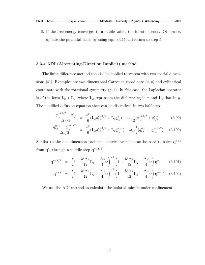
Ph.D. Thesis ––––––––– Jiajia Zhou ––––––––– McMaster University - Physics & Astronomy ––––––––– 2010
8. If the free energy converges to a stable value, the iteration ends. Otherwise,
update the potential fields by using eqn. (3.1) and return to step 5.
3.3.4 ADI (Alternating-Direction Implicit) method
The finite difference method can also be applied to system with two spatial dimen-
sions [41]. Examples are two-dimensional Cartesian coordinate (x, y) and cylindrical
coordinate with the rotational symmetry (ρ, z). In this case, the Laplacian operator
is of the form Lx + Ly, where Lx represents the differencing in x and Ly that in y.
The modified diffusion equation then can be discretized in two half-steps:
qn+1/2i,j − qni,j
∆s/2=
b2
6(Lxq
n+1/2i,j + Lyq
ni,j)− ωi,j
1
2(qn+1/2i,j + qni,j), (3.99)
qn+1i,j − q
n+1/2i,j
∆s/2=
b2
6(Lxq
n+1/2i,j + Lyq
n+1i,j )− ωi,j
1
2(qn+1i,j + q
n+1/2i,j ). (3.100)
Similar to the one-dimension problem, matrix inversion can be used to solve qn+1
from qn, through a middle step qn+1/2,
qn+1/2 =
(1− b2∆s
12Lx +
∆s
4ω
)−1 (1 +
b2∆s
12Ly −
∆s
4ω
)qn, (3.101)
qn+1 =
(1− b2∆s
12Ly +
∆s
4ω
)−1 (1 +
b2∆s
12Lx −
∆s
4ω
)qn+1/2. (3.102)
We use the ADI method to calculate the isolated micelle under confinement.
43

Ph.D. Thesis ––––––––– Jiajia Zhou ––––––––– McMaster University - Physics & Astronomy ––––––––– 2010
Chapter 4
Phase Behavior of AB/C Blends
The development of new polymeric materials is driven by increasingly complicated
requirements of advanced engineering, as well as by the desire to improve material
properties and reduce production cost. Beside synthesizing new types of homopoly-
mers and copolymers, blending different polymers provides another route to obtain
new materials [42, 43]. Polymer blends can have combinative and enhanced prop-
erties of their components. From a thermodynamic point of view, polymer blends
may be miscible, partially miscible, or immiscible. The physical properties of poly-
mer blends vary drastically in these different states. From this perspective, a good
understanding of the phase behavior of polymer blends is crucial. Because polymer
blends are composed of more than one element, their phase behavior is controlled
by a large number of parameters, such as chain lengths, monomer interactions and
polymer architectures. Due to the very large parameter space, theoretical study is
crucially important to understand the phase behavior and material properties in this
complex system.
Polymer blends containing block copolymers are of considerable interest because of
their remarkable structural properties [1]. One intriguing feature of block copolymers
is that they can self-assemble into periodic structures on the length scale of tens
of nanometer. The simplest block copolymer/homopolymer blend consists of diblock
copolymers and homopolymers that are chemically identical to one of the blocks of the
copolymers (AB/A system). There have been extensive studies on this system, both
44

Ph.D. Thesis ––––––––– Jiajia Zhou ––––––––– McMaster University - Physics & Astronomy ––––––––– 2010
in experiment and theory [44, 26, 45, 46, 47, 48, 49]. The phase diagrams of AB/A
blends exhibit both macrophase separation and microphase separations. The phase
behavior depends on the volume fraction of the homopolymer φH , and the relative
chain length of the homopolymer κ comparing to the copolymer. In general, there are
three different cases: (i) κ < 1. In this case, the chain length of the homopolymers
is less than that of the copolymers. The concentration of the short homopolymers is
roughly uniform throughout the region of the corresponding block, and the microphase
separation exists over a wide range of homopolymer concentration. (ii) κ ∼ 1. The
length of the homopolymers is comparable to the copolymers, and the homopolymers
will accumulate close to the center of the domain of the corresponding block. The
system tends to be microphase separated when the homopolymer concentration is
small, and undergoes macrophase separation at large homopolymer concentration.
(iii) κ > 1. The long homopolymers tend to be separated from the copolymers, and
the macrophase separation region appears dominantly in the phase diagram. The
above argument gives a qualitative description of the influence of the homopolymer
length, but a quantitative definition of these regions is still lacking.
More generally, it will be interesting to explore the system in which the homopoly-
mers are chemically distinct from both blocks of the copolymers (AB/C system).
Compared to the AB/A blends, one significant change is that the number of inter-
action parameters required to describe the system increases from one to three (the
three Flory-Huggins parameters χAB, χBC and χAC). Although the parameter space
of a general AB/C system is too large to be mapped out completely, it is possible to
compute some characteristic phase diagrams. These phase diagrams can be viewed
as a starting point to understand the complex phase behaviors of the blends, and also
to shed some light on possible future experiments.
45

Ph.D. Thesis ––––––––– Jiajia Zhou ––––––––– McMaster University - Physics & Astronomy ––––––––– 2010
In our study, we make some simplifications to a general AB/C blend. First we
assume the interactions between χBC > 0 and χAC = 0, which means the added
homopolymer C tends to accumulate in the region where A-block is occupied. This
setup resembles the AB/A system, but with the freedom of adjusting the interac-
tion between the homopolymer and the other block, while keeping χAB constant.
Furthermore, we consider only the classical phases: lamellae (LAM), cylinders on a
hexagonal lattice (HEX), and spheres on a body-centered cubic lattice (BCC). Com-
plex structures, such as close-packed spheres, perforated lamellae and bi-continuous
cubic phases, can also occur for certain parameters [26]. In general they are found
only in narrow regions between the classical phases. In this study, we are more in-
terested in the evolution of the ordered structure by varying different parameters,
therefore restrict ourselves to the three classical phases. The main interest of this
study is about asymmetric diblock copolymers, and we focus on the effect of the
homopolymer length and interaction parameters on the phase transition.
Our study can be viewed as an extension of the work of Matsen [45] and Janert and
Schick [46]. Matsen examined the AB/A system in the weakly segregated region. One
interesting phenomena occurs when blending A homopolymers to diblock copolymers
where A is the majority component. The blend starts with hexagonal structure, and
changes to lamellar structure when small amount of homopolymer are added, and
then switches back to hexagonal structure with more homopolymers added. We will
give a detailed analysis of this phenomenon and its origin. Janert and Schick also
studied AB/A blends and focused on the effect of the homopolymer chain length.
But their blends consist of symmetric diblock copolymers, while our work extends to
the asymmetric copolymers.
46

Ph.D. Thesis ––––––––– Jiajia Zhou ––––––––– McMaster University - Physics & Astronomy ––––––––– 2010
4.1 Phase diagrams
We solve the self-consistent equations in the grand canonical ensemble using the
spectral method. For each blend parameters, we calculate the free energy for dif-
ferent morphologies and the one with lowest free energy is the stable structure. Al-
though we work in the grand-canonical ensemble, we present our results in terms
of the canonical variables. For a general AB/C system, there are six parameters
(κ, fA, φH , χABN,χBCN,χACN) controlling the phase behavior. We set χACN = 0
as discussed before, which results a parameter space of five dimensions. We plot
our results using two-dimensional phase diagrams, with the abscissa always being
the homopolymer concentration φH . These figures can be viewed as two-dimensional
cross-sections of the five-dimensional parameter space.
Figure 4.1 shows a typical phase diagram for the blend with parameters χABN =
11.0, χBCN = 12.0, χACN = 0 and κ = 1.0, plotted in the φH-fA plane. This phase
diagram is similar to the results from Matsen [45] because the difference between
χABN and χBCN is small, thus our system resembles the AB/A system. Differ-
ent phases are labelled as DIS (disordered or homogeneous), LAM (lamellae), HEX
(cylinders on a hexagonal lattice), BCC (spheres on a body-centered cubic lattice) and
2-phase (macrophase separation). These short-handed notations are used throughout
this thesis.
Depending on the diblock copolymer composition, the blends undergo different
morphology transitions when the homopolymer concentration increases. Two different
phase sequences exist, distinguished by whether the macrophase separation appears
after large amount of homopolymer are added. When A is the minority component,
the pure diblock copolymers favor a structure which has curved interfaces to adopt
the volume asymmetry between A and B. When small amount of homopolymer is
added, the blend exhibits a transition to a structure with less curved interfaces (BCC
47

Ph.D. Thesis ––––––––– Jiajia Zhou ––––––––– McMaster University - Physics & Astronomy ––––––––– 2010
0.2
0.3
0.4
0.5
0.6
0.7
0 0.1 0.2 0.3 0.4 0.5 0.6 0.7 0.8 0.9 1
f A
!H
DIS
BCC
HEX
LAM
HEX
BCC
2-phase
Figure 4.1: Phase diagram of AB/C blend with parameters χABN = 11.0, χBCN =12.0, χACN = 0 and κ = 1.0. The results are plotted in terms of the homopolymervolume fraction φH and the A-monomer fraction of the diblock fA. For clarity, onlythe largest 2-phase region is labeled.
48

Ph.D. Thesis ––––––––– Jiajia Zhou ––––––––– McMaster University - Physics & Astronomy ––––––––– 2010
to HEX, or HEX to LAM). When the concentration of homopolymers is increased to
certain degree , the homopolymers and copolymers are separated into at a macroscopic
scale. Each region is either homopolymer-rich or copolymer-rich. The fraction of
copolymer-rich regions shrink when more homopolymers are added into the blends,
and eventually the disordered phase is reached again when significant amount of
homopolymers are added.
The second scenario happens when A is the majority component of the diblock
copolymer. The signature of this case is the disappearance of the 2-phase region in
the phase diagram. Also, a reverse of phase transitions seems to occur when the
homopolymer concentration is low. For example, at fA = 0.55, the blend starts with
HEX structure for pure diblock copolymers. When small amount of homopolymers
are added, the blend changes to LAM structure and then switches back to HEX
structure. This feature appears as a bump of the transition lines in the φH-fA phase
diagram. When more homopolymers are added, the blend undergoes an unbinding
transition where the spacing of the ordered structure increases and eventually di-
verges at certain homopolymer concentration. Disordered phase is reached after the
unbinding transition.
In the following, we will discuss these two cases separately, and focus on the effect
of the homopolymer chain length and the monomer-monomer interactions.
4.2 Case I: fA < 0.5
For pure diblock copolymers with fA < 0.5, the A-monomers forms the core of
the structure and arranges on a Bravais lattice. When the homopolymers C are
added, there are more B-monomers and less A-monomers to interact with C, while
C-monomers have a repulsive interaction with B.
49

Ph.D. Thesis ––––––––– Jiajia Zhou ––––––––– McMaster University - Physics & Astronomy ––––––––– 2010
We study blends with parameters χABN = 11.0, χBCN = 14.0 and χACN = 0,
where the χBCN value is chosen higher than before in order to enhance the B/C
interaction. Fig. 4.2 shows a partial phase diagram near fA = 0.457 (this is the fA
value of LAM-HEX boundary for pure diblock copolymers). The phase boundaries
are two lines close to each other. Above the lines is the LAM phase and below is the
HEX phase, with the LAM-HEX coexistence in between the lines. Blends with three
different κ values are shown here to demonstrate the effect of the homopolymer length.
For short homopolymers (κ = 0.5), the value of fA at the LAM-HEX boundary
decreases as the homopolymer concentration increases. As the homopolymer length
becomes comparable to the copolymer, the slope of the phase boundary line become
positive. Longer homopolymers has even steeper positive slope, as shown in Fig. 4.2
for κ = 1.5.
0.451
0.452
0.453
0.454
0.455
0.456
0.457
0.458
0.459
0 0.002 0.004 0.006 0.008 0.01 0.012 0.014 0.016 0.018
f A
!H
"=0.5
"=1.0
"=1.5LAM
HEX
Figure 4.2: Phase diagram of AB/C blend with parameters χABN = 11.0, χBCN =14.0 and χACN = 0 for three different value of κ = 0.5, 1.0 and 1.5. The results areplotted in φH-fA axes.
50

Ph.D. Thesis ––––––––– Jiajia Zhou ––––––––– McMaster University - Physics & Astronomy ––––––––– 2010
This phenomena can be explained by the competition between the entropy and
energy. Since the A/C repulsive interaction is weaker than the B/C interaction,
homopolymers C mostly accumulate in the A-rich region. When the concentration of
the homopolymer increases, the homopolymers tend to increase the size of the A-rich
region and cause the blend to make a transition to a structure in which A-monomers
occupy more space compared to the B-monomers (HEX to LAM for fA is small).
In this way the extra space gained allows homopolymer C to settle, resulting the
negative slope of the phase boundary line.
Beside the entropy effect, there is also the energy effect which tends to reduce the
interaction energy by minimizing the contact between B and C. This will force the
A-rich region where C monomers are mostly accumulated to contract, and counteract
the expansion of A-rich region due to the entropy effect.
For short homopolymers, the entropy effect dominates, so the slope of the LAM-
HEX boundary is negative. As the length of the homopolymer approaches that of the
diblock, the repulsive interaction between B and C becomes stronger and the energy
effect becomes relevant. When homopolymers are added, the tendency of the A-
rich region to expand in order to accompany more homopolymers starts to compete
with its tendency to contract in order to minimize the unfavorable B/C contacts.
The energy effect becomes more important for longer homopolymers, thus causes the
LAM-HEX boundary line to have a positive slope.
We can also analyze the density profiles and calculate the size of the microstructure
to gain some insight of this phenomena. In Figure 4.3, we plot the period of the LAM
structure and the relative size of the A-rich region as a function of homopolymer
concentration φH . The parameter for the blends are χABN = 11.0, χBCN = 14.0,
χACN = 0 and fA = 0.46. In this calculation, the size of the A-rich region is measured
along the direction normal to the interface, and defined as twice the distance from
51

Ph.D. Thesis ––––––––– Jiajia Zhou ––––––––– McMaster University - Physics & Astronomy ––––––––– 2010
the lamellae center to the point where the second derivative of φA + φC is zero. Here
we want to emphasize that the period is calculated by minimizing the free energy for
a lamellar structure, and it does not necessarily mean that the LAM phase is stable.
We also plot the monomer-density of C for blends with the same parameters and
homopolymer concentration φH = 0.04, as shown in Figure 4.4. The density profiles
are plotted as a function of distance from the center of the A-rich region. Both figures
include three different length of the homopolymers κ = 0.5, 1.0, 1.5.
For the three different lengths of the homopolymers considered here, the period of
the LAM phase is a monotonic increasing function of the homopolymer concentration.
Although contraction of the period has been observed for LAM phase when very short
homopolymers are added [49], for homopolymers whose length is on the same order
as that of copolymer, the swelling of the ordered structure is more common. Since the
added homopolymer C tends to accumulate inside the A-rich region, we would also
expect the the relative size of A-rich region to increase as well. However, as shown
in Figure 4.3(b), the relative size of A-rich region actually decreases when small
amount of homopolymers are added, and the tendency of decreasing is more distinct
for longer homopolymers. This strange behavior can be explained by considering how
the homopolymers distribute. As seen in Figure 4.4, the high-weight homopolymers
(κ = 1.5) have a stronger segregation comparing to the short homopolymers (κ = 0.5).
The concentrated C monomers form a well-defined C-rich layer near the middle of
A-rich region, thus forming an A-attractive layer. The A monomers tend to gather
close to the C-rich layer, resulting in the pulling the A-B boundary close to the C-rich
layer.
Another point of view is from the previous discussion about the competition be-
tween the entropy and energy effect. Their influences on the size of the microstructure
have opposite trends; the entropy effect causes the ∆A/∆ to expand, whereas the en-
52

Ph.D. Thesis ––––––––– Jiajia Zhou ––––––––– McMaster University - Physics & Astronomy ––––––––– 2010
0.466 0.468
0.47 0.472 0.474 0.476 0.478
0.48 0.482
0 0.01 0.02 0.03 0.04 0.05 0.06 0.07
!A/!
"H
#=0.51.0
1.5
0.466 0.468
0.47 0.472 0.474 0.476 0.478
0.48 0.482
0 0.01 0.02 0.03 0.04 0.05 0.06 0.07
!A/!
"H
#=0.51.0
1.5
0.466 0.468
0.47 0.472 0.474 0.476 0.478
0.48 0.482
0 0.01 0.02 0.03 0.04 0.05 0.06 0.07
!A/!
"H
#=0.51.0
1.5
3.25
3.3
3.35
3.4
3.45
3.5
3.55
3.6
3.65
!
#=1.51.0
0.5
3.25
3.3
3.35
3.4
3.45
3.5
3.55
3.6
3.65
!
#=1.51.0
0.5
3.25
3.3
3.35
3.4
3.45
3.5
3.55
3.6
3.65
!
#=1.51.0
0.5
Figure 4.3: Spatial variables of LAM structure for AB/C blend with parametersχABN = 11.0, χBCN = 14.0, χACN = 0 and fA = 0.46. (a) Period of the LAMstructure ∆, measured in unit of Rg = Na2/6, as a function of the homopolymerconcentration φH . (b) The relative size of A-rich region ∆A, in unit of ∆, as afunction of φH .
0
0.001
0.002
0.003
0.004
0.005
0.006
0.007
0.008
0.009
0.01
0 0.2 0.4 0.6 0.8 1
!=0.5!=1.0!=1.5
Figure 4.4: C-monomer density profile for AB/C blend with parameters χABN = 11.0,χBCN = 14.0, χACN = 0, fA = 0.46 and φH = 0.04.
53

Ph.D. Thesis ––––––––– Jiajia Zhou ––––––––– McMaster University - Physics & Astronomy ––––––––– 2010
ergy effect tends to decrease ∆A/∆. When the homopolymer concentration is low, the
energy effect outplays entropy effect, causing ∆A/∆ to decrease. Longer homopoly-
mers have a stronger energy effect so ∆A/∆ has a sharper negative slope comparing
to the short homopolymers. As we add more homopolymers, the entropy effect even-
tually prevails, and ∆A/∆ starts to increase for all three lengths of homopolymers at
high homopolymer concentration.
It is easier to demonstrate the effect of the homopolymer length by plotting the
phase diagram in φH-κ axes. Figure 4.5 shows such a phase diagram for blends with
parameters χABN = 11.0, χBCN = 14.0, χACN = 0 and fA = 0.46.
0.8
0.9
1
1.1
1.2
1.3
1.4
0 0.02 0.04 0.06 0.08 0.1 0.12 0.14
!
"H
HEX
LAM
2-phase
Figure 4.5: Phase diagram of AB/C blend with parameters χABN = 11.0, χBCN =14.0, χACN = 0 and fA = 0.46. The results are plotted in φH-κ axes.
There are two regions of κ, each showing different phase behaviors. When κ <
0.85, LAM phase is stable until relatively high concentration of homopolymer. The
blend then macrophase separates into LAM-DIS coexisted phase. As κ > 0.85, the
blend makes the transition from LAM to HEX at a small value of φH . Semenov
54

Ph.D. Thesis ––––––––– Jiajia Zhou ––––––––– McMaster University - Physics & Astronomy ––––––––– 2010
[44] had argued this scenario as long homopolymers clumping together to form the
nucleus for the ordered structure. The blend then undergoes macrophase separation
at a higher homopolymer concentration.
13
13.5
14
14.5
15
0 0.01 0.02 0.03 0.04 0.05 0.06 0.07
! BCN
"H
HEX
LAM
2-phase
Figure 4.6: Phase diagram of AB/C blend with parameters χABN = 11.0, χACN = 0and κ = 1.0. The results are plotted in φH-χBCN axes.
The length of the homopolymer is one of many factors which can influence the
energy effect. Others include the three Flory-Huggins parameters and the A-monomer
fraction of the diblock fA. For the interaction parameters, it is the difference between
χACN and χBCN that matters. Figure 4.6 demonstrates this effect. While keeping
χACN constant, we vary χBCN from 13 to 15. There are also two ranges of χBCN
with different phase behaviors, similar to Figure 4.5. This is understandable since in
both scenarios, we are changing the interaction between B and C, either by varying
the number of C monomers, or changing the Flory-Huggins parameter between B and
C.
55

Ph.D. Thesis ––––––––– Jiajia Zhou ––––––––– McMaster University - Physics & Astronomy ––––––––– 2010
4.3 Case II: fA > 0.5
For blends in which A-monomers are the majority component, we will focus on
the transition bump at the LAM-HEX boundary, as shown in Fig. 4.1 near fA = 0.54.
We study the blends with parameters χABN = 11.0, χBCN = 12.0, χACN = 0. Fig.
4.7 shows a partial phase diagram around fA = 0.54 for three value of κ = 0.5, 1.0
and 1.5.
0.53
0.535
0.54
0.545
0.55
0.555
0.56
0.565
0.57
0 0.05 0.1 0.15 0.2
f A
!H
LAM
HEX
"=0.5
"=1.0
"=1.5
Figure 4.7: Phase diagram of AB/C blend with parameters χABN = 11.0, χBCN =12.0 and χACN = 0 for three different value of κ = 0.5, 1.0 and 1.5. The results areplotted in terms of φH and fA.
Comparing Figure 4.7 and Figure 4.2, we notice that the bump feature in the
phase transition lines for fA > 0.5. For short homopolymer (κ = 0.5), the value of fA
at the LAM-HEX boundary decreases as the homopolymer concentration increases.
As the homopolymer length becomes comparable to the copolymer, the slope of the
phase boundary is positive initially, and becomes negative after certain value of φH .
For κ = 1.0, this value is about 0.092. Longer homopolymer has even larger positive
56

Ph.D. Thesis ––––––––– Jiajia Zhou ––––––––– McMaster University - Physics & Astronomy ––––––––– 2010
slope, as shown in Fig. 4.7 for κ = 1.5, but there may not be a bump because the
macrophase separation appears before the plunge of the transition line.
We again plot the phase diagram in φH-κ axes in order to apprehend the effect of
the homopolymer length. Figure 4.8 shows such a phase diagram for the blend with
parameters χABN = 11.0, χBCN = 12.0, χACN = 0 and fA = 0.55. The fA is chosen
to be right above the value of HEX-LAM transition (fA = 0.543) for pure diblock
copolymers.
0.8
0.9
1
1.1
1.2
1.3
1.4
1.5
0 0.05 0.1 0.15 0.2 0.25 0.3 0.35 0.4
!
"H
HEX
LAM
2-phase
Figure 4.8: Phase diagram of AB/C blend with parameters χABN = 11.0, χBCN =12.0, χACN = 0 and fA = 0.55. The results are plotted in terms of the homopolymervolume fraction φH and the relative length of the homopolymer κ.
There are three regions of κ, each showing different phase behaviors. When κ <
0.8, HEX phase is stable until relatively high concentration of homopolymer. The
blend then macrophase separates into HEX-DIS coexisted phase. As 0.8 < κ < 1.1,
the blend makes the transition from HEX to LAM at a small value of φH and then
reverses the transition at a higher concentration. When more homopolymers are
added, the blend also undergoes macrophase separation. This is the region where the
57

Ph.D. Thesis ––––––––– Jiajia Zhou ––––––––– McMaster University - Physics & Astronomy ––––––––– 2010
bump appears in φH-fA plots. As κ > 1.1, the blend keeps the lamellar phase after
changing from HEX to LAM, and macrophase separates into LAM-DIS coexisted
phase when φH is large.
The reversion of phase transition is a distinct feature for fA > 0.5, in comparison
with the phase diagram for fA < 0.5 (Fig. 4.5). The difference is caused by the
different value of φH at which the system undergoes macrophase transition. When
small amount of homopolymers is added, the energy effect acts first and the blend
makes a transition to decrease the space occupied by the A-rich domain. In the fA >
0.5 case, the blend undergoes transition from HEX to LAM. When more homopolymer
is added, there are two ways to distribute the extra homopolymers. One way is for the
homopolymers to macrophase separated from the diblock copolymer, which accounts
for the appearance of 2-phase region at higher φH . The other way is to increase the
size of A-rich domain, if the entropy gain from increasing A-rich domain is more than
enough to compensate both the entropy penalty of reducing the B-rich region and the
energy effect. It is easier for blends with fA < 0.5 to take this routine because the
φH value for macrophase separation is low. As for fA > 0.5, it takes large amount
of homopolymer to reach the macrophase separation, so the second scenario happens
for fA > 0.5 as the blends reverse back to HEX phase as φH increases.
Figure 4.9 shows the effect of varying interaction parameter χBCN for the blend
with parameters χABN = 11.0, χACN = 0 and κ = 1.0. There are also three ranges
of χBCN with different phase behaviors, similar to Figure 4.8.
4.4 Summary
In this chapter, we constructed phase diagrams of AB/C blends using self-consistent
field theory. Our study has focused on the asymmetric diblock copolymer, especially
58

Ph.D. Thesis ––––––––– Jiajia Zhou ––––––––– McMaster University - Physics & Astronomy ––––––––– 2010
11.4
11.6
11.8
12
12.2
12.4
12.6
12.8
13
0 0.05 0.1 0.15 0.2 0.25 0.3 0.35 0.4
! BCN
"H
HEX
LAM
2-phase
Figure 4.9: Phase diagram of AB/C blend with parameters χABN = 11.0, χACN = 0and κ = 1.0. The results are plotted in terms of the homopolymer volume fractionφH and the interaction parameter χBCN .
those close to the LAM-HEX boundary. The influences of the homopolymer con-
centration, the homopolymer chain length and the interaction parameters, on the
phase behavior have been investigated. An interesting reversion of phase transition
has been described for fA > 0.5 case. In this study we only consider the classical
phases, and more complex structure are expected to appear in a small region between
the classical phases, but this should not change the qualitative picture of the phase
transition sequence.
59

Ph.D. Thesis ––––––––– Jiajia Zhou ––––––––– McMaster University - Physics & Astronomy ––––––––– 2010
Chapter 5
AB/C Blends with Attractive Interaction
One feature of AB/C blends studied in the previous chapter is that there are large
regions of macrophase separating in the phase diagram. From engineering point of
view, sometimes this is undesirable because most applications rely on the homoge-
neous property of the material. Therefore, the interactions between the homopoly-
mers and the diblock copolymers have to be controlled carefully.
The phase behavior of AB/C blends can be categorized into three cases, depend-
ing on the miscibility of C with respect to the AB diblock copolymers. If the ho-
mopolymer C is immiscible with both blocks A and B, the situation is simple: the
homopolymers will be separated from diblock copolymers. A more complex case in-
volves AB/C blends where the homopolymers C are immiscible with one block of the
diblock copolymers, but interact favorable with the other block [50, 51, 52, 53, 54].
This system is similar to the case of amphiphilic molecules in solution, which is im-
portant to understand the self-assembly of surfactants and lipids. A simple example
of this class of blends is that the homopolymers are chemically identical to one of
the blocks of the copolymers, i.e., an AB/A blend. Binary AB/A blends have been
extensively studied theoretically [26, 44, 45, 46] and experimentally [47, 48, 49]. The
phase diagrams of AB/A blends show the coexistence of macrophase separation and
microphase separation, and the addition of the homopolymers tends to stabilize some
complex ordered structures. The previous chapter was devoted to this case.
60

Ph.D. Thesis ––––––––– Jiajia Zhou ––––––––– McMaster University - Physics & Astronomy ––––––––– 2010
Another interesting case occurs for blends consisted of C homopolymers that are
miscible with both the A and B blocks. The miscible nature of the blends may pro-
vide potential applications which rely on homogeneity of the material. Theoretically
and practically, the extension to the attractive interactions between compounds may
lead to new phenomena and create new materials. In general, miscible blends are
characterized by homogeneous phases. However, phase separation can be induced by
differential monomer-monomer interactions. An example is found in ternary blends
composed of A/B/C homopolymers where all three binary pairs are miscible. A
closed-loop immiscible region is found in the phase diagram [55, 56, 57, 58]. In
cases that the attractive interaction between A/C is much stronger than that of B/C
and A/B, A and C homopolymers tend to be separated from B. On the other hand,
macroscopic phase separation of A and B cannot take place for AB/C blends, because
A and B are chemically bonded together. Similar to the case of block copolymers,
AB/C blends can reduce their free energy through microphase separation. Indeed,
the microphase separation of AB/C blends has been observed in experiment of Chen
et al. [28]. These authors investigated AB/C blends where the interactions between
each pair of segments are favorable. Their experiments revealed a phase diagram with
a closed microphase separation loop, despite the fact that the C homopolymers have
attractive interactions with both blocks of the copolymers.
In this chapter, we present a theoretical study of the phase behavior of diblock
copolymer/homopolymer blends. The study focuses on the case where the homopoly-
mers attract to one block much more strongly than to the other block of the diblock
copolymers. We use the Gaussian chain model for the polymers, and apply the ran-
dom phase approximation (RPA) to examine the stability limits of the homogeneous
phase, leading to both macrophase and microphase separation transition. While the
RPA calculates the stability boundary of the homogeneous phase, we are also inter-
61

Ph.D. Thesis ––––––––– Jiajia Zhou ––––––––– McMaster University - Physics & Astronomy ––––––––– 2010
ested in the morphological details inside the microphase separation region. For this
purpose, self-consistent field theory is employed. Various representative phase dia-
grams are constructed to illuminate the general trends in the phase behavior by vary-
ing the homopolymer length and monomer-monomer interaction parameters. Com-
parison with available experiments is given.
5.1 Random phase approximation
The random phase approximation analysis of a polymer blend [59, 17, 60, 61]
starts with an external potential field uα acting on the α monomer. Assuming that
the external fields are small, the density response to the external potential, δφα, can
be written in the Fourier space as a linear function of the external potential,
δφα(q) = − 1
kBT
∑β
Sαβ(q)uβ(q), (5.1)
where Sαβ(q) is the Fourier transform of the density-density correlation between α
and β monomers. Here we have used the fact that functions depend on the wave
vector q only through its magnitude q ≡ |q| because of the isotropic symmetry of a
homogeneous phase.
The interaction between the monomers can be taken into account through the
mean-field approximation. To this end, the effective potential acting on the αmonomer
is written in the form,
ueffα (q) = uα(q) + kBT
∑β 6=α
χαβδφβ + η, (5.2)
where the second term accounts for the mean-field interaction between α and β
monomers, and η is a potential required to assure the incompressible condition
∑α
δφα(q) = 0. (5.3)
62

Ph.D. Thesis ––––––––– Jiajia Zhou ––––––––– McMaster University - Physics & Astronomy ––––––––– 2010
The random phase approximation assumes that the density response δφα is given
by the effective potential,
δφα(q) = − 1
kBT
∑β
Sαβ(q)ueffβ (q), (5.4)
where Sαβ(q) is the Fourier transform of the density-density correlation when the
external potential vanishes.
Equations (5.1)-(5.4) form a set of simultaneous equations for the unknowns δφα
and η. By solving these equations, the correlation functions Sαβ can be found in
terms of Sαβ and χαβ. The final results are [61]
SAA(q) = SAA(q)− 2[W3(q)/S3(q)]χBC/F (q) (5.5)
SAB(q) = SAB(q)− [W3(q)/S3(q)]
×(χAB − χBC − χAC)/F (q) (5.6)
SBB(q) = SBB(q)− 2[W3(q)/S3(q)]χAC/F (q) (5.7)
where
Sαβ(q) = Sαβ(q)− tα(q)tβ(q)/S3(q), (5.8)
tα(q) =∑β
Sαβ(q), (5.9)
S3(q) =∑α,β
Sαβ(q), (5.10)
W3(q) = 2SAB(q)SBC(q)SAC(q)
+SAA(q)SBB(q)SCC(q)− SAA(q)S2BC(q)
−SBB(q)S2AC(q)− SCC(q)S2
AB(q), (5.11)
F (q) = 2[SAB(q)χAB + SBC(q)χBC + SAC(q)χAC ]
+[W3(q)/S3(q)]2χABχBC + 2χBCχAC
+2χACχAB − χ2AB − χ2
BC − χ2AC + 1, (5.12)
63

Ph.D. Thesis ––––––––– Jiajia Zhou ––––––––– McMaster University - Physics & Astronomy ––––––––– 2010
Here we only express SAA, SAB and SBB explicitly because the other Sαβ can be
written as combinations of these three due to the incompressibility and the symmetry
of Sαβ = Sβα.
The free energy of AB/C blends can be written as a Landau expansion about the
homogeneous state in terms of the density fluctuations δφα,
F − Fhom
(ρ0V kBT/N)=
1
2!(2π)
∫S−1αβ (q)δφα(q)δφβ(−q)dq + · · · ,
=1
2!(2π)
∫λk(q)|δψk(q)|2dq + · · · , (5.13)
where S−1αβ (q) is the inverse of the correlation function Sαβ(q). Here we have neglected
terms with order higher than two, and the second-order term can be further written
in a quadratic form, where λk(q) are eigenvalues of the matrix S−1αβ (q). The stability
of the homogeneous phase depends on the sign of eigenvalues λk(q). When λk(q) > 0,
the contribution of any fluctuations to the free energy is always positive, so the
homogeneous phase is stable. When λk(q) < 0, the fluctuations reduce the free
energy and the homogeneous phase is unstable.
Normally, the inverse of the correlation function S−1αβ (q) is a 3×3 matrix for the
AB/C blends. The incompressible condition reduces the order of the matrix by one.
The spinodal line is determined by the condition that the smaller eigenvalue goes to
zero. Typical plots of λk(q) are shown in Fig. 5.1. In general, one of the eigenval-
ues λ1(q) is always positive, while the other one λ2(q) approaches zero when χACN
changes.
The macrophase separation is characterized by λ2(q) → 0 at q = 0. This is
shown in Figure 5.1(a) for blends with κ = 1.0, fA = 0.8, φH = 0.2, χABN = 15,
χBCN = 0 and different χACN values. The eigenvalue λ2(q) has a minimum at
q = 0, and the minimum value approaches zero when χACN increases. When λ2(q)
becomes negative, any small density fluctuations with q = 0 decrease the free energy,
64
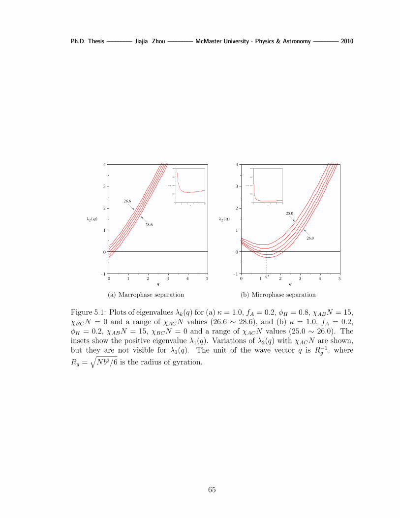
Ph.D. Thesis ––––––––– Jiajia Zhou ––––––––– McMaster University - Physics & Astronomy ––––––––– 2010
26.6
28.6
(a) Macrophase separation
q*
26.0
25.0
(b) Microphase separation
Figure 5.1: Plots of eigenvalues λk(q) for (a) κ = 1.0, fA = 0.2, φH = 0.8, χABN = 15,χBCN = 0 and a range of χACN values (26.6 ∼ 28.6), and (b) κ = 1.0, fA = 0.2,φH = 0.2, χABN = 15, χBCN = 0 and a range of χACN values (25.0 ∼ 26.0). Theinsets show the positive eigenvalue λ1(q). Variations of λ2(q) with χACN are shown,but they are not visible for λ1(q). The unit of the wave vector q is R−1
g , where
Rg =√Nb2/6 is the radius of gyration.
65

Ph.D. Thesis ––––––––– Jiajia Zhou ––––––––– McMaster University - Physics & Astronomy ––––––––– 2010
leading to a growth of fluctuations with macroscopic wavelength. This corresponds
to a macrophase separation between the diblock-rich phase and homopolymer-rich
phase.
On the other hand, the diblock copolymers in the blend introduce the possibility
of microphase separation. A microphase transition is characterised by the eigenvalue
λ2(q) → 0 at some finite q∗ > 0. This is shown in Figure 5.1(b) for blends with
κ = 1.0, fA = 0.2, φH = 0.2, χABN = 15, χBCN = 0 and different χACN values.
The Fourier mode with nonzero wave number q∗ becomes unstable upon increasing
χACN , leading to the formation of ordered structure with length scale of (q∗/2π)−1.
This is in contrast to Figure 5.1(a) where the Fourier mode q = 0 is destabilized first.
The six parameters (κ, fA, φH , χABN,χBCN,χACN) characterising the AB/C blends
lead to a huge phase space. Some restrictions are needed so that the phase behavior
can be described. We will keep κ = 1.0 for the RPA calculation, which means the
homopolymer C has the same degree of polymerization as the diblock copolymer AB.
Furthermore, we will assume χBCN = 0, which represents the case where the A/C
interaction is much stronger than the B/C interaction.
Fig. 5.2(a) shows a typical phase diagram in the φH-χACN plane. The parameters
are fA = 0.2 and χABN = 2. The solid lines and dotted lines represent, respectively,
the stability limits for the macrophase separation transition (χACN)macro and mi-
crophase separation transition (χACN)micro.
The blends are disordered around χACN = 0 and φH = 1, and ordered phases
appear at both χACN > 0 and χACN < 0. In the region where χACN > 0, increasing
χACN induces an instability to either macrophase separation or microphase sepa-
ration, depending on the blend composition and copolymer asymmetry. For blends
with a minority of homopolymers, microphase separation occurs first when χACN is
66

Ph.D. Thesis ––––––––– Jiajia Zhou ––––––––– McMaster University - Physics & Astronomy ––––––––– 2010
Micrphase
DIS
Macrophase
(a) χABN = 2
Macrophase
DIS
Microphase
(b) χABN = 30
Figure 5.2: Phase diagrams for blends with parameters κ = 1.0, fA = 0.2, χBCN = 0and (a) χABN = 2, (b) χABN = 30. The solid and dotted lines represent the stabilitylimits for macrophase and microphase separation transition, respectively. Regions ofmacrophase separation, microphase separation and disordered states are labeled byMacrophase, Microphase and DIS.
increased. However, when the composition of the homopolymers increases to certain
value, the blend undergoes macrophase separation when χACN is increased. The crit-
ical composition for blends with fA = 0.2 is φH ≈ 0.2. The shape of the stability lines
also suggests that, for small φH value, both (χACN)macro and (χACN)micro decrease
with increasing φH , while (χACN)macro increases with increasing φH at large φH value.
The former case suggests that the composition of the diblock copolymer in the blend
suppresses the phase transition, which is known as the compatibilizing effect of the
block polymers [62].
On the other hand, the microphase separation also occurs in the region where
χACN is negative. Since the interaction between the blocks χABN = 2, the pure
diblock copolymers are in the disordered state. The stability line for the microphase
separation approaches φH = 0 axis infinitely close when χACN has a large negative
value. It is interesting that for a homogeneous diblock copolymer melt, adding a small
67

Ph.D. Thesis ––––––––– Jiajia Zhou ––––––––– McMaster University - Physics & Astronomy ––––––––– 2010
amount of homopolymers C which has a strong attractive interaction with one of the
blocks will induce the phase separation. Upon increasing φH , (χACN)micro increases
sharply at first, then decreases after φH ≈ 0.25.
A similar phase diagram for blends with χABN = 30 is shown in Fig. 5.2(b). In
this case, the pure diblock copolymers are in the ordered state. This leads to the
convergence of the two microphase separation regions at χACN > 0 and χACN < 0.
Another perspective to understand the phase transition is to plot the phase di-
agram in the φH-fA plane for fixed interaction parameters. Fig. 5.3 shows phase
diagrams for blends with χABN = 2 and different values of χACN . They can be
viewed as cross-sections pictures of Fig. 5.2(a) at different values of χACN . At
χACN = 30, because of the strong repelling interaction between A/C, a large region
of macrophase separation exists, while a small region of microphase separation oc-
curs near the φH = 0 axis. As χACN decreases, the macrophase separation region
shrinks and eventually disappears at a negative value of χACN . At the same time,
a closed-loop microphase separation region appears, as can be seen from Fig. 5.3(c)
and 5.3(d). Qualitatively, this closed immiscible loop corresponds to the one observed
in experiments [28].
The closed-loop microphase separated region emerges at large negative value of
χACN , and also seems to expand with decreasing χACN . For a fixed copolymer
asymmetry fA, the lowest requirement of the homopolymer composition φmin to reach
the microphase transition is reduced when χACN decreases. This can be shown in
Figure 5.4, which plots the minimum value of φmin to reach the close-loop as a function
of χACN . When χACN decreases, the close-loop of microphase separation appears at
χACN ≈ −36 for χABN = 2, and at χACN ≈ −44 for χABN = −2. For the same
χACN value, the blend with a lower χABN value requires more copolymer composition
to reach the microphase transition.
68

Ph.D. Thesis ––––––––– Jiajia Zhou ––––––––– McMaster University - Physics & Astronomy ––––––––– 2010
Macrophase
DIS
Microphase
(a) χACN = 30
Macrophase
DIS
(b) χACN = 5
Microphase
DIS
(c) χACN = −50
Microphase
DIS
(d) χACN = −90
Figure 5.3: Phase diagrams for AB/C blends in φH-fA plane. The parameters areκ = 1.0, χABN = 2 and χBCN = 0. The solid and dotted lines represent thetransitions for macrophase and microphase separation, respectively.
69

Ph.D. Thesis ––––––––– Jiajia Zhou ––––––––– McMaster University - Physics & Astronomy ––––––––– 2010
Figure 5.4: The minimum homopolymer composition φmin to reach the immisci-ble close-loop as a function of χACN . The parameters are α = 0.5, f = 0.5 andχBCN = 0. The solid and dashed lines present the case χABN = 2 and χABN = −2,respectively.
70

Ph.D. Thesis ––––––––– Jiajia Zhou ––––––––– McMaster University - Physics & Astronomy ––––––––– 2010
5.2 Self-consistent field theory
Because of its simplicity, random phase approximation provides a convenient
method to calculate the order-disorder transition for various parameter sets, but
it is difficult to apply RPA to the order-order transition. On the other hand, self-
consistent field theory has been proved a powerful method to determine the mi-
crostructures of polymer blends [19, 22, 25, 26, 45, 46]. Therefore, it is desirable to
apply self-consistent field theory to the study of the phase behavior of AB/C blends
with attractive interactions.
Similar to previous chapter, we consider only the classical phases: lamellae (LAM),
cylinders on a hexagonal lattice (HEX), and spheres on a body-centered cubic lattice
(BCC). Complex structures, such as close-packed spheres, perforated lamellae and
bi-continuous cubic phases, can also occur for certain parameters [26]. These non-
classical phases were usually found in narrow regions between the classical phases. In
this study, we are more interested in the evolution of the phase diagram by varying
different parameters, therefore we restrict ourselves to the three classical phases.
Fig. 5.5(a) shows a phase diagram in the φH-fA plane for blends with κ = 1.0,
χABN = 11, χBCN = 0 and χACN = −30. In this case, the value of χABN is large
enough so the diblock copolymer melt is in an ordered state. The results should
converge to the pure diblock results as the homopolymer concentration goes to zero,
which is the case as shown in Figure 5.5(a). The phase behavior shown in Figure
5.5(a) is typical for the case where the homopolymers attract strongly to one of the
blocks (χACN = −30). This attractive interaction drives the C homopolymers to
the A-domains, leading to larger regions of ordered phases for mediated homopoly-
mer concentrations. For comparison, a phase diagram for the blends with κ = 1.0,
χABN = 11, χBCN = 12 and χACN = 0 is presented in Fig. 5.5(b) (from Chapter
71

Ph.D. Thesis ––––––––– Jiajia Zhou ––––––––– McMaster University - Physics & Astronomy ––––––––– 2010
4). Here the parameters are chosen in such a way that the C monomers accumulate
inside the A-rich region for both cases.
These two phase diagrams display similar features when the homopolymer concen-
tration is small. In this region, the majority of the blend is diblock copolymers and
adding small amount of homopolymers should preserve the morphologies. When the
homopolymer concentration becomes large, these two phase diagrams exhibit different
phase behavior. For the case shown in Fig. 5.5(b), where the interaction parameter
χBCN is positive, two possible scenarios of phase behavior appear. When fA is large,
only one disordered phase is stable. The blend tends to undergo unbinding transition
where the spacing of the ordered structure increases and eventually diverges at certain
homopolymer concentration [26, 45, 46]. When fA is small, macroscopic phase sepa-
ration becomes an option. Adding more homopolymers induces a macrophase separa-
tion transition, in which the blend separates into copolymer-rich and homopolymer-
rich regions. On the other hand, for the case shown in Fig. 5.5(a), where χACN has
a large negative value, only one disordered phase is permitted. When the homopoly-
mer concentration is large, the blends exhibit neither the unbinding transition nor
the macrophase separation. This behavior is due to the strong attractive interaction
between the A and C monomers. As the homopolymer concentration is increased
close to unity, both cases reach a disordered phase.
When all three binary pairs are miscible, the AB/C blends exhibit another type
of phase behavior. Fig. 5.6 shows a typical phase diagram for this case with κ = 1.0,
χABN = 2, χBCN = 0 and χACN = −40. In this case the blends are in a disordered
phase at φH = 0 and φH = 1. Ordered phases occur in a closed-loop region, as
indicated by the RPA analysis. Inside the closed-loop, different ordered structures
are found. The order-order transitions between these structures are controlled largely
by the homopolymer concentration φH .
72

Ph.D. Thesis ––––––––– Jiajia Zhou ––––––––– McMaster University - Physics & Astronomy ––––––––– 2010
(a) χACN = −30
(b) χACN = 12
Figure 5.5: Phase diagrams of AB/C blends with parameters κ = 1.0, χABN = 11,χBCN = 0, and (a) χACN = −30, (b) χACN = 12. The superscripts of HEX andBCC phase denote the components that form the cylinders and spheres near thelattice centers. There are regions of 2-phase coexistence between the ordered phases.
73

Ph.D. Thesis ––––––––– Jiajia Zhou ––––––––– McMaster University - Physics & Astronomy ––––––––– 2010
Figure 5.6: Phase diagram of AB/C blends with parameters κ = 1.0, χABN = 2,χBCN = 0 and χACN = −40. The dotted line shows the RPA result.
There are two critical points at which all ordered phases converge on the order-
disorder transition boundary. For the parameters used here, one point is located at
(φH = 0.083, fA = 0.58), and the other one at (φH = 0.33, fA = 0.21). The order-
disorder transition is a second-order transition at these two critical points, while the
transition is first-order elsewhere. The nature of the order-disorder transition (ODT)
can be understood by considering the third-order term in the free energy expansion.
A first-order phase transition occurs when a non-zero third-order term is present.
In the case of a phase transition from the disordered phase to the BCC phase, the
third-order term does not vanish in general. Therefor a first-order ODT is expected.
At the critical points, the ODT corresponds to a direct transition from the disordered
phase to a lamellar phase. In this case the symmetry of the lamellar phase ensures
the vanishing of the third-order term, resulting in a second-order ODT [63].
It is important to point out the limitation of the present theory. The mean-field
approach used here approximates the fluctuating potential by a thermal averaged
74

Ph.D. Thesis ––––––––– Jiajia Zhou ––––––––– McMaster University - Physics & Astronomy ––––––––– 2010
potential. This assumption becomes inaccurate near the order-disorder transition,
where the fluctuations are large. The fluctuations can shift the position of the phase
boundary, and may change the second-order ODT into a weakly first-order transition
[64, 65].
When the homopolymer concentration is increased, the AB/C blends change from
a disordered phase to BCC, HEX and LAM phases. This sequence of phase transition
can be understood by examining how homopolymers are distributed in the diblock
melt. Since the interaction between A and B are at χABN = 2, which is well below
the ODT value of 10.5 for symmetric diblocks, the pure diblock copolymers are in
a disordered state. When small amount of homopolymers are added to the system,
due to their strong attraction to A-blocks, the homopolymers are distributed around
the A-blocks, resulting in an effective segregation of the A-B blocks. Ordered phases
emerge when this effective segregation becomes strong enough. Another way to pic-
ture this effect is to take the homopolymers as the core-forming agents of micelles in a
diblock copolymer melt. The appearance of the spherical phase as the homopolymers
are added can be regarded as the ordering of these micelles. The key observation
here is that the reduction of interaction energy from A-C segregation is sufficient to
overcome the entropy loss. At the strong-segregation limit, a similar mechanism for
the formation of reverse structures has been discussed by Semenov [44].
At higher homopolymer concentration, the volume of A/C domain increases. The
packing requirement of larger A/C domains leads to a change of the interfaces between
A/C and B, such that the interfaces are curved more towards the B-domain. This
mechanism lead to order-order phase transitions from BCC to HEX, and then from
HEX to LAM phases. After the LAM structure, adding more homopolymers induces
the phase transition to HEX, and then to BCC, where the HEX and BCC both have
75

Ph.D. Thesis ––––––––– Jiajia Zhou ––––––––– McMaster University - Physics & Astronomy ––––––––– 2010
B-blocks as the central components. Eventually, a disordered phase is reached when
sufficient amount of homopolymers are added.
In order to explore the effect of the A/C interactions, phase diagrams are con-
structed for different A/C interactions, either by changing the molecular-weight of C
homopolymers or by changing the value of the Flory-Huggins parameter χAC . Fig.
5.7(a), 5.6 and 5.7(b) show the evolution of the phase diagrams with increasing κ
(κ = 0.5, 1.0 and 1.5). Alternatively, the phase diagrams in Fig. 5.8(a), 5.6 and
5.8(b) demonstrate the progression as χACN decreases (χACN = −35, −40 and −45)
at fixed κ. It is obvious that the qualitative feature of the phase diagram stays the
same in these phase diagrams. The main difference is the size of the closed-loop or-
dered phase region. Increasing the interaction will increase the area of the parameter
space in which the blend is ordered.
Experimentally, several groups had studied blends with attractive interactions [28,
66]. In Ref. [28], Chen et al. studies the phase diagrams of PVPh-b-PMMA/PVP
blends, where all three binary pairs, PVPh/PMMA, PMMA/PVP and PVP/PVPh,
are miscible. Their setup closely resembles the blends studied in this work. They
found a closed-loop microphase separation region surrounded by disordered phases.
The three classical phases were also observed inside the closed-loop. The position of
the closed-loop is similar to our theoretical prediction. Furthermore, the transition
sequence of ordered phases from their experiments is consistent with our theoretical
phase diagrams.
In a slightly different experiment setup [66], Tirumala et al. studied a triblock
copolymer/homopolymer blend (PEO-PPO-PEO/PAA), where PAA interacts selec-
tively to the end-block PEO. Upon increasing homopolymer concentration, they ob-
served a phase sequence of disordered phase to lamellae, then to cylinders consisted
76

Ph.D. Thesis ––––––––– Jiajia Zhou ––––––––– McMaster University - Physics & Astronomy ––––––––– 2010
(a) κ = 0.5
(b) κ = 1.5
Figure 5.7: Phase diagrams of AB/C blends with parameters χABN = 2, χBCN = 0,χACN = −40 and (a) κ = 0.5, (b) κ = 1.5.
77

Ph.D. Thesis ––––––––– Jiajia Zhou ––––––––– McMaster University - Physics & Astronomy ––––––––– 2010
(a) χACN = −35
(b) χACN = −45
Figure 5.8: Phase diagrams of AB/C blends with parameters κ = 1.0, χABN = 2,χBCN = 0, and (a) χACN = −35, (b) χACN = −45.
78

Ph.D. Thesis ––––––––– Jiajia Zhou ––––––––– McMaster University - Physics & Astronomy ––––––––– 2010
of PPO, then back to disordered phase. This transition sequence is again consistent
with our theoretical predictions.
5.3 Summary
In this chapter, we have investigated the phase behavior of blends composed of
AB diblock copolymers and C homopolymers. Two theoretical methods have been
employed to construct the phase diagrams. By using the random phase approxima-
tion, the stability limits of the homogeneous phase are obtained. The phase dia-
grams are characterized by the coexistence of macrophase separation and microphase
separation. When the interaction between A/C is repulsive, increasing χACN will
induce the transition from disordered phase to ordered phase, and the property of
the transition depends on the homopolymer concentration. In general, blends with
low homopolymer concentration tend to undergo microphase separation transition,
whereas macrophase separation occurs at high homopolymer concentration. When
the interaction parameter χACN becomes attractive, the macrophase separation dis-
appears while the microphase separation can still occur when the magnitude of χACN
is large. The microphase separation is caused by the strong attraction between the
homopolymers to one of the blocks of the diblock copolymers. The difference be-
tween the A/C and B/C interactions leads to the spatial separation of B monomers
from the A/C monomers, but the chemical connections between A and B prevent
the macrophase separation. The microphase separation manifests itself in the φH-fA
phase diagram in a closed-loop region.
The detailed morphologies inside the closed-loop are calculated using self-consistent
field theory. The RPA results provide a guidance to explore the parameter space.
Three classical ordered phases (LAM, HEX and BCC) are included in the current
79
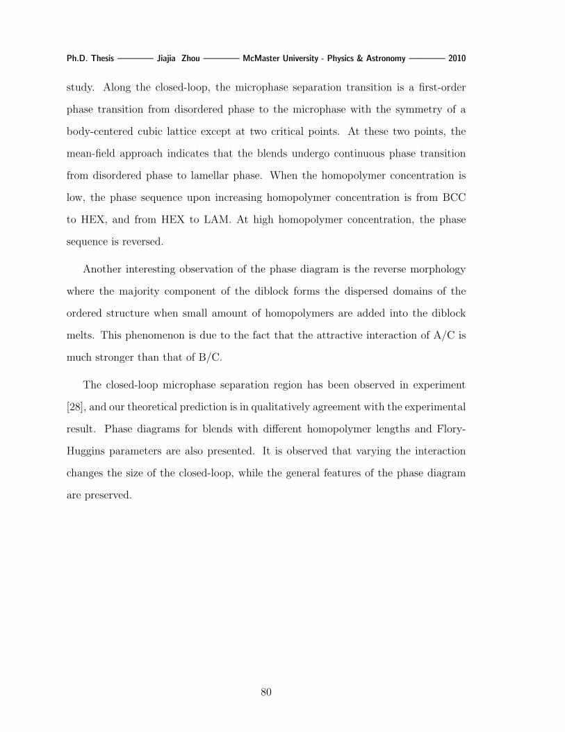
Ph.D. Thesis ––––––––– Jiajia Zhou ––––––––– McMaster University - Physics & Astronomy ––––––––– 2010
study. Along the closed-loop, the microphase separation transition is a first-order
phase transition from disordered phase to the microphase with the symmetry of a
body-centered cubic lattice except at two critical points. At these two points, the
mean-field approach indicates that the blends undergo continuous phase transition
from disordered phase to lamellar phase. When the homopolymer concentration is
low, the phase sequence upon increasing homopolymer concentration is from BCC
to HEX, and from HEX to LAM. At high homopolymer concentration, the phase
sequence is reversed.
Another interesting observation of the phase diagram is the reverse morphology
where the majority component of the diblock forms the dispersed domains of the
ordered structure when small amount of homopolymers are added into the diblock
melts. This phenomenon is due to the fact that the attractive interaction of A/C is
much stronger than that of B/C.
The closed-loop microphase separation region has been observed in experiment
[28], and our theoretical prediction is in qualitatively agreement with the experimental
result. Phase diagrams for blends with different homopolymer lengths and Flory-
Huggins parameters are also presented. It is observed that varying the interaction
changes the size of the closed-loop, while the general features of the phase diagram
are preserved.
80

Ph.D. Thesis ––––––––– Jiajia Zhou ––––––––– McMaster University - Physics & Astronomy ––––––––– 2010
Chapter 6
Bulk micelles
The linkages between the incompatible segments make the diblock copolymer an
ideal model system to study the self-assembly. One interesting example is the mi-
cellization of diblock copolymers blended with homopolymers which are chemically
identical to one of the blocks (AB/A blends). The covalent bonds between the incom-
patible blocks lead to the formation of aggregates. Similar phenomenon occurs for
other amphiphilic molecules, such as the segregation of the surfactants in water and
the bilayer formation of lipids. A good understanding of the micellization in diblock
copolymer/homopolymer blends not only is important from the fundamental polymer
physics point of view, it may also provide guidance to more complicated biological
systems.
Consider a melt of A homopolymers and we gradually add diblock copolymers AB
into the system. At very low copolymer concentration, the diblock copolymers stay as
isolated chains in the homopolymer matrix, and the physical properties of the blend
vary smoothly. As more copolymers are added, the B-blocks of the copolymers tend
to cluster together in order to avoid the unfavored contact with the A homopolymers,
thus forming micellar aggregates. The copolymer concentration at which the micelles
start to emerge is called the critical micelle concentration (cmc) [67]. The physical
properties of the blend also experience abrupt changes due to a sharp increase of
the micelle number. Various micelle morphologies, including lamellar, cylindrical,
and spherical micelles, can be obtained. The preferred morphology is decided by
81

Ph.D. Thesis ––––––––– Jiajia Zhou ––––––––– McMaster University - Physics & Astronomy ––––––––– 2010
several factors, such as the copolymer concentration, diblock asymmetry, the copoly-
mer/homopolymer lengths, and the monomer-monomer interaction. Micelles formed
by copolymers consist of a core of the B-blocks surrounded by a corona of the A-
blocks. The corona may or may not be swollen by the A homopolymers. These
aggregates typically have a characteristic size which is much larger than those of a
single molecule, but they do not become macroscopic objects. This makes micelles
suitable for potential medical applications, particularly in drug delivery [68].
A large number of theories and simulations have been developed over the years in
order to model the micelle formation. Several authors have derived an analytic form
of the total free energy as a function of the thermodynamic variables, such as the
number of copolymers per micelle, the core and corona sizes. Leibler [69] studied the
case of long homopolymer chains that do not penetrate into the corona of the micelle.
Leibler considered spherical geometry, and the model was extended to cylindrical and
lamellar micelles by Shull et al. [70]. On the other hand, when homopolymers have
a length compatible to that of copolymers, they can swell the corona of the micelles.
Leibler et al. [71] considered the formation of spherical micelles in this scenario, and
later the theory was revised to study the transition between cylindrical and spherical
micelles by Mayes et al. [72]. These methods clearly illustrate the fundamental
physics of the micellization, but in order to make quantitative comparison with the
experiments, more elaborate methods are required.
Self-consistent field theory is a powerful theoretical method to model polymer
systems, and its molecular-level accuracy can provide detailed information about
the micelle structure. Several researches have been conducted to the study of the
micellization [73, 74, 75, 76, 77, 78, 79]. Duque [76] employed the theory with an
additional constraint that permits the examination of intermediate structures. Chang
et al. [77] used a pressure difference to stabilize the micelle. Greenall et al. [78, 79]
82

Ph.D. Thesis ––––––––– Jiajia Zhou ––––––––– McMaster University - Physics & Astronomy ––––––––– 2010
used a method of varying the size of simulation box. These studies have greatly
enriched our understanding of the micelle formation. However, there still lacks a
thorough investigation of the shape transition by changing various parameters.
In this chapter, we use self-consistent field theory to model an isolated micelle in
dilute systems of diblock copolymers AB with homopolymers A. We consider three
different micelle morphologies: lamellar, cylindrical and spherical. We focus on the
shape transition of the micelle and the roles of the diblock asymmetry, the homopoly-
mer length and the interaction parameter.
6.1 Isolated micelles
Here we introduce the notations for the binary blend of AB/A. Most of them are
consistent with previous notations for AB/C blends.
The blend is composed of diblock copolymers with a chain length N , and ho-
mopolymers with a chain length κN in a volume of V . The copolymer has a fraction
fA of A-monomers, and fB(= 1 − fA) of B-monomers. The volume fraction for A-
monomer in the homopolymer, A- and B-monomer in the copolymer are φhA, φcA and
φcB, respectively. The copolymer concentration is φc = φcA + φcB. (This should not
be confused with concentration of the C-monomer used before, but since we do not
have a C component, here the subscript c stands for copolymer). We also assume the
blend is incompressible and all monomers have the same volume ρ−10 . The monomer-
monomer interaction is characterized by the standard Flory-Huggins parameter χ.
We formulate the theory in the grand-canonical ensemble. The incompressibility per-
mits the choice of setting the chemical potential for homopolymers to be zero, and
the controlling parameter is the copolymer chemical potential µc, or equivalently, the
activity zc ≡ exp(µc)/κ.
83
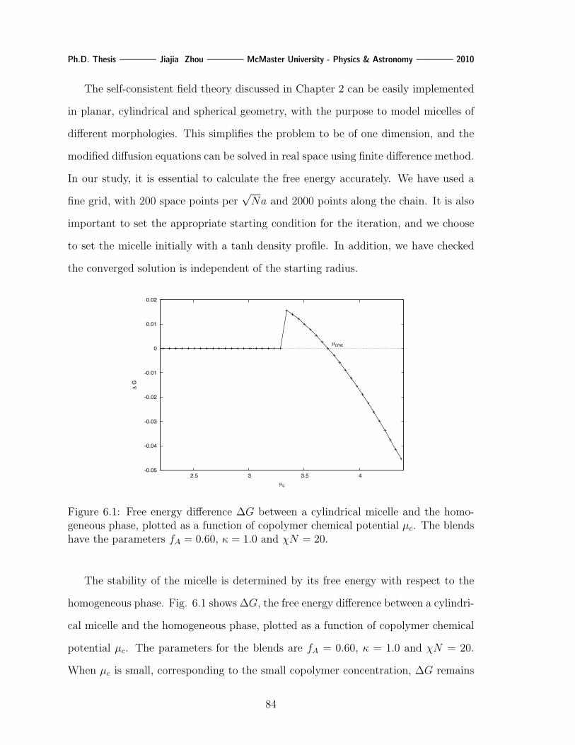
Ph.D. Thesis ––––––––– Jiajia Zhou ––––––––– McMaster University - Physics & Astronomy ––––––––– 2010
The self-consistent field theory discussed in Chapter 2 can be easily implemented
in planar, cylindrical and spherical geometry, with the purpose to model micelles of
different morphologies. This simplifies the problem to be of one dimension, and the
modified diffusion equations can be solved in real space using finite difference method.
In our study, it is essential to calculate the free energy accurately. We have used a
fine grid, with 200 space points per√Na and 2000 points along the chain. It is also
important to set the appropriate starting condition for the iteration, and we choose
to set the micelle initially with a tanh density profile. In addition, we have checked
the converged solution is independent of the starting radius.
-0.05
-0.04
-0.03
-0.02
-0.01
0
0.01
0.02
2.5 3 3.5 4
! G
µc
µcmc
Figure 6.1: Free energy difference ∆G between a cylindrical micelle and the homo-geneous phase, plotted as a function of copolymer chemical potential µc. The blendshave the parameters fA = 0.60, κ = 1.0 and χN = 20.
The stability of the micelle is determined by its free energy with respect to the
homogeneous phase. Fig. 6.1 shows ∆G, the free energy difference between a cylindri-
cal micelle and the homogeneous phase, plotted as a function of copolymer chemical
potential µc. The parameters for the blends are fA = 0.60, κ = 1.0 and χN = 20.
When µc is small, corresponding to the small copolymer concentration, ∆G remains
84

Ph.D. Thesis ––––––––– Jiajia Zhou ––––––––– McMaster University - Physics & Astronomy ––––––––– 2010
around zero. When µc approaches µcmc from below, ∆G increases slightly, and then
becomes negative when µc is greater than µcmc. Here we define cmc as the copolymer
concentration of the bulk when the excess free energy becomes negative. By using
this definition, we have neglected the translational entropy of the micelles. Since we
are mostly concerned with the blends of small copolymer concentrations, the density
of micelles is small and the interactions between micelles are negligible. Once the µcmc
is found, the critical micelle concentration can be calculated from the bulk relation,
µcκ
=lnφcκ− ln(1− φc) + fBχN(1− 2fBφc) (6.1)
0
0.2
0.4
0.6
0.8
1
0 0.5 1 1.5 2 2.5 3
!
r
Rcore Rcore+Lcorona
!hA!cA!cB
Figure 6.2: Density profiles for an isolate cylindrical micelle. The blend has theparameters fA = 0.60, κ = 1.0, χN = 20 and µc = 3.87.
One of the advantages of self-consistent field method is that detailed density pro-
files can be obtained for the isolated micelle. Fig. 6.2 shows the density profiles for the
same blend in Fig. 6.1 with µc = 3.87. With this knowledge, we are able to compute
the geometrical variables of the micelle, such as the core and corona sizes, and the
material properties of the micelle, such as the number of copolymer/homopolymer
85

Ph.D. Thesis ––––––––– Jiajia Zhou ––––––––– McMaster University - Physics & Astronomy ––––––––– 2010
within the micelle. For the core radius, a simple definition would be the point where
φcA(r) = φcB(r). However, this definition breaks down in the weak segregation region
when sufficient amount of homopolymers are present inside the core. We opt to first
calculate the radius of gyration of the core. For spherical micelles, it has a form
R2g,core =
∫r2(φcB(r)− φbcB)dV∫(φcB(r)− φbcB)dV
, (6.2)
where φbcB is the B-block concentration of copolymers in the bulk phase which has to
be removed to isolate the core. The core radius then can be computed from Rg,core,
R2g,core =
3
5R2
core. (6.3)
Following a similar procedure, we can compute the radius of gyration of the corona,
R2g,corona =
∫r2(φcA(r)− φbcA)dV∫(φcA(r)− φbcA)dV
, (6.4)
where φbcA is the A-block concentration of copolymers in bulk. The corona thickness
is related to Rg,corona by
R2g,corona =
3
5
(Rcore + Lcorona)5 −R5core
(Rcore + Lcorona)3 −R3core
. (6.5)
For lamellar and cylindrical micelles, similar forms can be obtained.
In order to better understand the material distribution inside the micelle, we define
two more variables for the micelle. The first one is the excess copolymers, defined as
Ω =1
Vmicelle
∫ Rmicelle
0(φc(r)− φbc)dV, (6.6)
where Rmicelle = Rcore + Lcorona and φbc is the copolymer concentration in bulk. This
variable characterizes the number of copolymers that are segregated. The second one
is the penetrating homopolymer which has a form
Θ =1
Vmicelle
∫ Rmicelle
0φhA(r)dV. (6.7)
86

Ph.D. Thesis ––––––––– Jiajia Zhou ––––––––– McMaster University - Physics & Astronomy ––––––––– 2010
This variable describes the number of homopolymers which penetrate inside the mi-
celles, which is a good indication for the degree of swelling.
6.2 Results and Discussions
In general, the critical micelle concentration for certain morphology is a function
of the diblock asymmetry fA, the homopolymer/copolymer length ratio κ, and the
interaction parameter χN . The cmc for different morphologies can be obtained from
self-consistent field theory, and the preferred micelle geometry is the one with the
lowest cmc. Since the chemical potential is a monotonic function of the copolymer
concentration in dilution solution, the same result can be obtained by comparing the
copolymer chemical potential.
We begin by examining the dependence of fA, while keeping κ and χN constant.
Before we present our results, it is intuitive to repeat the results from the scaling
theory [70] for comparison. In Fig. 6.3, the value of µcmc/(χN)1/3 for different
geometries are plotted as functions of copolymer asymmetry fA. The micelle geometry
is expected to be lamellar for fA < 0.65, cylindrical for 0.65 < fA < 0.87, and
spherical for fA > 0.87. Also, the value of fA at which the shape transition occurs
is independent of χN , due to the coincidence that µcmc for different geometries have
the same prefactor (χN)1/3.
In the inset of Fig. 6.4, the critical micelle concentrations are plotted as a function
of fA for blends with κ = 1.0 and χN = 20. The curves for different geometries are
close to each other and it is difficult to distinguish them, but the trend of increasing
cmc as fA is increased can be seen. When fA is increased while the total length of the
copolymer kept constant, the length of B-block is reduced, which effectively reduces
the incompatibility between copolymers and homopolymers. At the same time, the
87

Ph.D. Thesis ––––––––– Jiajia Zhou ––––––––– McMaster University - Physics & Astronomy ––––––––– 2010
0.4
0.5
0.6
0.7
0.8
0.9
1
1.1
1.2
1.3
1.4
0.5 0.6 0.7 0.8 0.9 1
µcm
c/(!N
)1/3
fA
lamcyl
sph
Figure 6.3: Dependence of µcmc on the copolymer asymmetry fA as derived from thescaling method. Three morphologies are plotted: lamellar (blue solid line), cylindrical(green, dashed line) and spherical (red dotted line).
length of A-block is increased, which improves the solubility of the copolymers in the
homopolymers. Thus a higher copolymer concentration is required for the micelles to
form.
The shape transition can be more clearly seen from the chemical potential plot,
as shown in Fig. 6.4. µcmc is a decreasing function of fA for cylindrical and spherical
micelles, except when the copolymer becomes very asymmetric. The µcmc for bilayers
also has a small negative slope, in contrast to the scaling theory. For more symmetric
copolymers, the chemical potential is much lower for the lamellar micelles than for
the cylindrical and spherical micelles, indicating the bilayer structure is favored. As
fA increases, µcmc decreases. The slopes of the decrease are different for different
geometries, as the curve for spherical micelles decreases most sharply, and that for
the lamellar is more flat. The comparison between µcmc indicates a trend of shape
transition: lamellar → cylindrical → spherical. This tendency can be explained by
a simple geometrical argument; as fA increases, the ratio between the volume of the
88

Ph.D. Thesis ––––––––– Jiajia Zhou ––––––––– McMaster University - Physics & Astronomy ––––––––– 2010
3.4
3.5
3.6
3.7
3.8
3.9
4
4.1
0.5 0.55 0.6 0.65 0.7 0.75
µcm
c
fA
3.4
3.5
3.6
3.7
3.8
3.9
4
4.1
0.5 0.55 0.6 0.65 0.7 0.75
µcm
c
fA
3.4
3.5
3.6
3.7
3.8
3.9
4
4.1
0.5 0.55 0.6 0.65 0.7 0.75
µcm
c
fA
-3-2.5
-2-1.5
-1-0.5
0
0.5 0.55 0.6 0.65 0.7 0.75
log(! c
mc)
fA
Figure 6.4: Dependence of µcmc on the copolymer asymmetry fA for blends withχN = 20 and κ = 1.0. The critical micelle concentrations are plotted in the inset.Notation as in Fig. 6.3.
corona (A-block) and core (B-block) becomes larger, causing the interfaces between
the A/B blocks to curve more towards the core. For κ = 1.0 and χNc = 20, shape
transitions happen at fA = 0.54 and fA = 0.65.
In Fig. 6.5, plots similar to those in Fig. 6.4 are shown except the length ratio
of homopolymer/copolymer is changed to κ = 2.0. In contrast to the scaling results,
the transition points move towards more asymmetric copolymers. In this case, they
are at fA = 0.59 and fA = 0.70.
In Fig. 6.6, we increase the incompatibility between A/B monomers, χN = 50,
while keeping the homopolymer length the same. The change of χNc has a pronounced
effect on cmc (notice the difference in y-scale of Fig. 6.4 and 6.6 insets). Similar to
Fig. 6.5, the transition points also shift to more asymmetric copolymers.
The shape transition of the micelle can also be induced by varying the homopoly-
mer molecular weight. We choose to study the blends with fA = 0.70 and χN = 20.
For such an asymmetric diblock copolymer, the lamellar structure is unstable, so only
89

Ph.D. Thesis ––––––––– Jiajia Zhou ––––––––– McMaster University - Physics & Astronomy ––––––––– 2010
3.1
3.2
3.3
3.4
3.5
3.6
3.7
3.8
0.5 0.55 0.6 0.65 0.7 0.75
µcm
c
fA
3.1
3.2
3.3
3.4
3.5
3.6
3.7
3.8
0.5 0.55 0.6 0.65 0.7 0.75
µcm
c
fA
3.1
3.2
3.3
3.4
3.5
3.6
3.7
3.8
0.5 0.55 0.6 0.65 0.7 0.75
µcm
c
fA
-3
-2.5
-2
-1.5
-1
-0.5
0.5 0.55 0.6 0.65 0.7 0.75
log(! c
mc)
fA
Figure 6.5: Dependence of µcmc and φcmc on the copolymer asymmetry fA for blendswith χN = 20 and κ = 2.0. Notation as in Fig. 6.3.
5
5.2
5.4
5.6
5.8
6
0.55 0.6 0.65 0.7 0.75 0.8
µcm
c
fA
5
5.2
5.4
5.6
5.8
6
0.55 0.6 0.65 0.7 0.75 0.8
µcm
c
fA
5
5.2
5.4
5.6
5.8
6
0.55 0.6 0.65 0.7 0.75 0.8
µcm
c
fA
-8-7-6-5-4-3-2
0.55 0.6 0.65 0.7 0.75 0.8
log(! c
mc)
fA
Figure 6.6: Dependence of µcmc and φcmc on the copolymer asymmetry fA for blendswith χN = 50 and κ = 1.0. Notation as in Fig. 6.3.
90

Ph.D. Thesis ––––––––– Jiajia Zhou ––––––––– McMaster University - Physics & Astronomy ––––––––– 2010
cylindrical and spherical micelles are considered. In Fig. 6.7, the critical micelle con-
centrations are plotted as functions of κ. Since the difference in cmc between different
homopolymer lengths is considerably larger than those between different shapes for a
given homopolymer length, we also plot the difference of cmc in the inset to demon-
strate the transition point more clearly. The micelle undergoes the transition from
spherical to cylindrical at around κ = 2.0.
To better understand the mechanism of the shape transition, we plot the mi-
celle core radius, the corona thickness, the excess copolymers and the penetrating
homopolymers in the micelle. In Fig. 6.8(a), the radius of the core consisted mostly
of B-blocks of the copolymers are shown as a function of κ. The copolymer chain
configurations in the core are notably different for the two geometries. In the core
of the cylindrical micelles, the B chains are only slightly extended from their Gaus-
sian configuration (the unperturbed rms end-to-end distance for the B-block with
fB = 0.3 is 0.22√Na). When the homopolymer length is increased, the B chains are
stretched further, but in a more slow manner. This is because more copolymers are
segregated into the micelle, as shown in Fig. 6.8(c). This effect counters the increase
of core radius and provides some release for the B chains. For the spherical micelle,
similar trends of the core radius and excess copolymers are found, but comparing to
the cylindrical micelles, B-blocks are severely elongated in the spherical micelle.
The corona of the micelle consists of mostly A-blocks of the copolymer, swollen
by A homopolymers. The corona thickness is shown in Fig. 6.8(b). Although the
corona thickness appears to be much larger than the length of the unperturbed A-
block (0.34√Na), the A-blocks are not strongly stretched due to the presence of A
homopolymers. The difference between the two morphologies lies in the degree of
swelling, as shown in Fig. 6.8(d). The cylindrical micelle has more homopolymers
penetrating into the corona than the spherical micelle. Those homopolymers can help
91
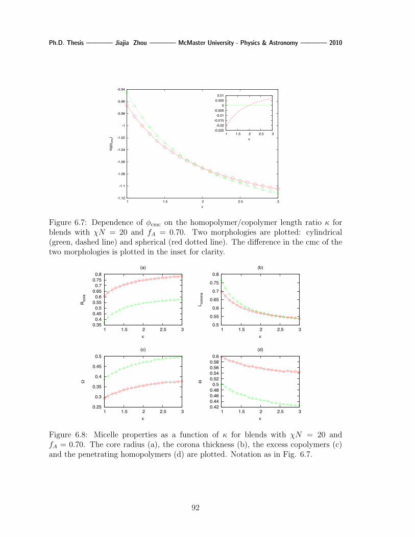
Ph.D. Thesis ––––––––– Jiajia Zhou ––––––––– McMaster University - Physics & Astronomy ––––––––– 2010
-1.12
-1.1
-1.08
-1.06
-1.04
-1.02
-1
-0.98
-0.96
-0.94
1 1.5 2 2.5 3
log(! c
mc)
"
-0.025-0.02
-0.015-0.01
-0.005 0
0.005 0.01
1 1.5 2 2.5 3"
Figure 6.7: Dependence of φcmc on the homopolymer/copolymer length ratio κ forblends with χN = 20 and fA = 0.70. Two morphologies are plotted: cylindrical(green, dashed line) and spherical (red dotted line). The difference in the cmc of thetwo morphologies is plotted in the inset for clarity.
0.25
0.3
0.35
0.4
0.45
0.5
1 1.5 2 2.5 3
!
"
(c)
0.42 0.44 0.46 0.48
0.5 0.52 0.54 0.56 0.58
0.6
1 1.5 2 2.5 3
#
"
(d)
0.35 0.4
0.45 0.5
0.55 0.6
0.65 0.7
0.75 0.8
1 1.5 2 2.5 3
R cor
e
"
(a)
0.5
0.55
0.6
0.65
0.7
0.75
0.8
1 1.5 2 2.5 3
L cor
ona
"
(b)
Figure 6.8: Micelle properties as a function of κ for blends with χN = 20 andfA = 0.70. The core radius (a), the corona thickness (b), the excess copolymers (c)and the penetrating homopolymers (d) are plotted. Notation as in Fig. 6.7.
92

Ph.D. Thesis ––––––––– Jiajia Zhou ––––––––– McMaster University - Physics & Astronomy ––––––––– 2010
to relax the A-blocks in the corona. When κ is increased, the size of the homopolymers
becomes bigger comparing to the micelle, and it is more difficult for the homopolymers
to penetrate inside the corona. Therefore, the corona length decreases as κ increases.
The deformation of the polymer chain in both the core and the corona are remark-
ably different for the two geometries. Comparing the spherical micelle, the B-blocks
in the core of cylindrical micelle are less stretched, and the A-blocks in the corona
is more relaxed. This contrast results in a shape transition from spherical micelle to
cylindrical micelle as the homopolymer length is increased, as demonstrated in Fig.
6.7. Similar effect has been discussed in Ref. [72] for the case κ < 1.
Change in the micelle morphology can also take place by varying the interaction
parameter χN . We consider blends with parameters fA = 0.7 and κ = 1.0. The
critical micelle concentrations and some properties of the micelle are plotted in Fig.
6.9 and 6.10. A change of morphology from spherical to cylindrical micelle is exhibited
when the χN is increased, similar to the case when κ is increased. However, there
are some notable differences. First, the cmc changes more rapidly by varying χN .
The value of cmc is reduced by two orders of magnitude when χN changes from 20
to 40, while the cmc has the same order when κ changes from 1 to 2. Varying the
homopolymer length is to change the surrounding of the micelle, while changing the
interaction parameter directly alters the incompatibility between the A/B blocks of
the copolymers, so latter has a much profound effect on the cmc. Second, as shown
in Fig. 6.10(b), there appears to be a minimum in the corona thickness when χN is
increased. At the weak segregation region when χN is small, the corona is strongly
swollen by the A homopolymers. As χN increases, the repelling between A and B
monomers pushes A homopolymers away from the corona, subsequently reducing the
corona thickness. As χN becomes larger and reaches the strong segregation region,
the interfacial energy becomes important. Both the A/B blocks of copolymers have
93

Ph.D. Thesis ––––––––– Jiajia Zhou ––––––––– McMaster University - Physics & Astronomy ––––––––– 2010
-4.5
-4
-3.5
-3
-2.5
-2
-1.5
-1
-0.5
20 25 30 35 40 45 50
log(! c
mc)
"Nc
-0.025-0.02
-0.015-0.01
-0.005 0
0.005 0.01
0.015 0.02
20 25 30 35 40 45 50"Nc
Figure 6.9: Dependence of φcmc on the interaction parameter χN for blends withκ = 1.0 and fA = 0.70. Two morphologies are plotted: cylindrical (green, dashedline) and spherical (red dotted line). The difference in the cmc of the two morphologiesis plotted in the inset for clarity.
0.25 0.3
0.35 0.4
0.45 0.5
0.55 0.6
0.65
20 25 30 35 40 45 50
!
"N
(c)
0.35
0.4
0.45
0.5
0.55
0.6
20 25 30 35 40 45 50
#
"N
(d)
0.35 0.4
0.45 0.5
0.55 0.6
0.65 0.7
0.75 0.8
0.85 0.9
20 25 30 35 40 45 50
R cor
e
"N
(a)
0.62 0.64 0.66 0.68
0.7 0.72 0.74 0.76 0.78
20 25 30 35 40 45 50
L cor
ona
"N
(b)
Figure 6.10: Micelle properties as a function of χN for blends with κ = 1.0 andfA = 0.70. The core radius (a), the corona thickness (b), the excess copolymers (c)and the penetrating homopolymers (d) are plotted. Notation as in Fig. 6.9.
94
Ph.D. Thesis ––––––––– Jiajia Zhou ––––––––– McMaster University - Physics & Astronomy ––––––––– 2010
to be stretched in order to reduce the surface per copolymer, therefore the corona
thickness starts to increase. This is similar to the case of diblock melts, where the
period of the order structure increases as χN increase.
Changes of the micelle morphology in dilute poly(styrene-butadiene)/polystyrene
solutions were observed experimentally by Kinning et al. [80]. They have examined
the case of varying the homopolymer length, and their results are in agreement with
the trend shown in Fig. 6.9.
6.3 Summary
In this chapter, we have investigated the shape transition of an isolated micelle
formed in the AB/A blends. Self-consistent field theory has been employed to com-
pute the critical micelle concentration for three different morphologies: lamellar, cylin-
drical and spherical. By comparing the cmc for different shapes, the preferred micelle
geometry is determined. Several factors can influence the micelle morphology, and
we have explored the diblock asymmetry, the homopolymer/copolymer length ratio
and the monomer-monomer interaction. It is found the micelle undergoes a sequence
of shape transitions, lamellar → cylindrical → spherical, when the A-block of the
copolymer becomes longer. For asymmetric copolymers with a large A-block, the
transition from spherical to cylindrical micelle is expected when the homopolymer
length is increased. A similar trend appears when the repulsive interaction between
different monomers become stronger. The mechanism of the shape transition can
be explained by examining the chain deformation inside the micelle. Valuable infor-
mation can be obtained from the theory, such as the geometrical dimensions of the
micelle, and the distribution of the polymers. These properties are closely related to
the controlling parameters. By varying these parameters, micelle with required shape
95

Ph.D. Thesis ––––––––– Jiajia Zhou ––––––––– McMaster University - Physics & Astronomy ––––––––– 2010
and size may be obtained for potential applications. Since it is inconceivable and
expensive for experimentalists to explore the parameter space by trial-and-error, the-
oretical study is crucially important to understand the underlying cause and provide
guidance for the experiments.
It is important to point out the limitation of the present approach. Since we have
neglected the translational entropy of the micelles, the critical micelle concentrations
calculated are only valid when the copolymer concentration is small. Also, for lamel-
lar and cylindrical micelles, we only considered the ideal case, while in reality, infinite
long cylinders and infinite broad bilayers can not be formed. The ends of the cylin-
ders or the edges of the lamellae will have a contribution to the free energy, so the
points of shape transition needed be shifted accordingly. Nevertheless, by comparing
the minimum copolymer concentration required for micellization in three geometries
under ideal conditions, we have obtained the trends we expect to observe in dilute
systems of diblock copolymer with homopolymers. Due to the computational com-
plexity, we only considered the three simplest geometries. Irregular micelle shape
may occur under certain conditions, such as under confinement, which is the subject
of next chapter.
96

Ph.D. Thesis ––––––––– Jiajia Zhou ––––––––– McMaster University - Physics & Astronomy ––––––––– 2010
Chapter 7
Micelles in Thin Film
Polymer thin films are widely used in technology and industry. Applications of
polymer thin films include protective surface coatings, birefringent elements in optical
devices, and printing circuits in flexible solar cells. Films made by blending differ-
ent homopolymers/copolymers provide an economical route to obtain new product
with enhanced properties. In general, the usage of polymer films requires the surface
properties to be homogeneous, but polymer blends tend to phase separate. Copoly-
mers can be used as compatibilizers to induce miscibility in polymer mixtures, but
they tends to form aggregates when the concentration exceeds the critical micelle
concentration (cmc).
Polymer thin films can also be viewed as polymer blends under planar confinement.
For copolymer melts, planar confinement can induce novel morphologies which are not
available in bulk system [81, 82, 83]. The phase behavior is determined by the relation
between the size of confinement and the natural spacing of the structure. When these
two sizes are compatible, bulk structures are preserved; otherwise, new morphologies
like perforated lamellae can be formed. Similarly, the confinement can also influence
the micelle formation in diblock copolymer/homopolymer blends, and the important
factor is the ratio between the micelle dimensions and the size of confinement. When
the degree of confinement is small, the micelle reacts by slightly shrinking its size.
As the confinement becomes compatible to the micelle size, the micelle formation
97
Ph.D. Thesis ––––––––– Jiajia Zhou ––––––––– McMaster University - Physics & Astronomy ––––––––– 2010
becomes unfavorable. This results in an increase of the critical micelle concentration
[84, 85] or shape change.
In order to better understand the micelle formation in thin film, we study the mi-
celle shape change in diblock copolymer/homopolymer films. As we have discussed in
Chapter 6, micelles can have different morphologies in bulk system: bilayers, cylinders
and spheres. Only the planar micelles are commensurate with the thin film geometry,
while the other two undergo deformation when the degree of confinement increases.
For simplicity, we choose to focus on the spherical micelles in this chapter.
Several parameters control the micelle formation. In the bulk system, the mi-
cellization depends primarily on the copolymer architecture and monomer-monomer
interactions. In the thin film, the confinement introduces the effect of structure frus-
tration and surface interaction. The degree of structure frustration depends on the
relationship between the micelle size and film thickness. If the two are incomparable,
the aggregate must deviate from its equilibrium shape to relieve the imposed frus-
tration. Even change of micelle morphology can be induced when the confinement
is strong. Beside the geometry confinement, the other important factor in thin film
is the surface selectivity. The interaction between monomers and hard surfaces can
be neutral or preferential. The selective surface interactions also can cause deviation
from the structures observed in the bulk.
In this chapter, we use self-consistent field theory to study the shape of a single
micelle formed in the diblock copolymer/homopolymer (AB/A) blends. In Section
7.1, we incorporate the hard-surface effect in the SCFT framework. The deformation
of a spherical micelle is discussed in Section 7.2, and the effect of various parameters
are elucidated.
98

Ph.D. Thesis ––––––––– Jiajia Zhou ––––––––– McMaster University - Physics & Astronomy ––––––––– 2010
7.1 Hard-surface effect
To model the spherical micelles under planar confinement, we adapt a cylindrical
coordinate system (x = r, z) which has rotational symmetry with respect to z-axis.
The z-axis is perpendicular to the film surfaces, which are located at z = 0 and
z = D. Fig. 7.1 shows a schematic setup of the coordinate system.
O
z
D
x
Figure 7.1: Coordinate system for modeling the micelle formation in AB/A films.
In previous chapters, the incompressibility condition is enforced in the self-consistent
field theory. The total monomer density∑φα(r) = 1 everywhere. Under planar con-
finement, the top and bottom surface are impenetrable, which requires the monomer
density to vanish at the surface. A common method to solve this problem is to use
a profile φ0(r) that is 1 everywhere except close to the surface. Close to the surface,
the density varies continuously from 0 to 1 over a short distance of τ . The choice of
φ0(r) in the surface layer is not important, and we use the one proposed by Meng
and Wang [86] to enhance numerical stability,
φ0(r) =
[exp[4τz/(τ2−z2)]−1exp[4τz/(τ2−z2)]+1
]20 ≤ z ≤ τ
1 τ ≤ z ≤ D − τ[exp[4τ(D−z)/(τ2−(D−z)2)]−1exp[4τ(D−z)/(τ2−(D−z)2)]+1
]2D − τ ≤ z ≤ D.
(7.1)
The incompressibility constraint can be rewritten as
∑α
φα(r) = φ0(z). (7.2)
99

Ph.D. Thesis ––––––––– Jiajia Zhou ––––––––– McMaster University - Physics & Astronomy ––––––––– 2010
The total density profile near the surface is plotted in Fig. 7.2 for τ = 0.15Rg.
0
0.2
0.4
0.6
0.8
1
0 0.02 0.04 0.06 0.08 0.1 0.12 0.14
! 0(z
)
z
Figure 7.2: Total monomer density near the hard surface for τ = 0.15Rg.
The surface interaction is represented by a surface field H(r). For simplicity, a
short-range, linear field is used:
H(r) =
Γl(1− z/τ) 0 ≤ z ≤ τ
0 τ ≤ z ≤ D − τ
Γu[1− (D − z)/τ ] D − τ ≤ z ≤ D
(7.3)
The constant Γl and Γu are used to characterize the surface selectivity for the lower
and upper surfaces, respectively. In our notation, a positive value of Γ corresponds to
the attractive interaction to A-monomer (or a repulsive interaction to B-monomer).
The surface interaction adds another term in the field equations
ωA(r) = χNφB(r)−H(r) + η(r), (7.4)
ωB(r) = χNφA(r) +H(r) + η(r). (7.5)
100

Ph.D. Thesis ––––––––– Jiajia Zhou ––––––––– McMaster University - Physics & Astronomy ––––––––– 2010
The surface contribution to the total free energy is
fs = − 1
V
∫0≤z≤τ
dV H(r)[φA(r)− φB(r)] +∫D−τ≤z≤D
dV H(r)[φA(r)− φB(r)](7.6)
The self-consistent equations are solved in the real-space using the ADI method
[41]. In this chapter, we focus on the case that the homopolymer and copolymer have
the same length, so κ = 1. The blends have intermediate segregation at χN = 20.
7.2 Results and discussion
We present the results using two-dimension color plots. Fig. 7.3 shows the
monomer densities for a single spherical micelle under confinement. The three plots
correspond to the (a) B-block of the copolymer; (b) A-block of the copolymer and (c)
A-homopolymer. The light color corresponds to larger value of concentration.
The parameters are fA = 0.7, κ = 1, φc = 0.1 and χN = 20. The separation
between the surfaces are 4√Nb which is larger than the natural size of the micelle.
The surface selectivity is neutral so Λl = Λu = 0. The micelle consists of a core of the
B-blocks of the copolymer, surrounded by a corona of A-blocks. There are also small
amounts of A-homopolymers swelling the corona, as shown in the φhA(r) profile.
Far away from the micelle, the concentrations are expected to reach the bulk
values. However, due to the presence of the two hard surfaces, the density profile is
not homogeneous along the z direction (see Fig. 7.4). Because of the total density
is less than 1 near the surface, this effectively reduces the A-B repulsive interaction
in the surface layer [45]. Therefore it is energetically favorable for copolymers to
accumulate close to the surfaces. Furthermore, the B-block has a stronger tendency
to swell the surface layer than the A-block. This is because the surfaces are neutral, so
there are no differences between a diblock copolymer chain and a homopolymer chain
101

Ph.D. Thesis ––––––––– Jiajia Zhou ––––––––– McMaster University - Physics & Astronomy ––––––––– 2010
0 0.5 1 1.5 2 2.5 3 3.5 4
0
0.5
1
1.5
2
2.5
3
3.5
4
0.06
0.08
0.1
0.12
0.14
0.16
0.18
0.2
0 0.5 1 1.5 2 2.5 3 3.5 4
0
0.5
1
1.5
2
2.5
3
3.5
4
0
0.05
0.1
0.15
0.2
0.25
0 0.5 1 1.5 2 2.5 3 3.5 4
0
0.5
1
1.5
2
2.5
3
3.5
4
0.5
0.55
0.6
0.65
0.7
0.75
0.8
0.85
Rx
Rz
!cB(r)
!cA(r)
!hA(r)
Figure 7.3: Monomer density profiles for a spherical micelle formed in the AB/Afilms. The length unit is
√Nb.
102

Ph.D. Thesis ––––––––– Jiajia Zhou ––––––––– McMaster University - Physics & Astronomy ––––––––– 2010
for the surface. From the entropy point of view, both ends of the copolymer have the
equal probability to be found near the surface. This corresponds to an enrichment
of the minority-component of the copolymer (B-block for fA = 0.7). This effect is
demonstrated in Fig. 7.4.
0
0.002
0.004
0.006
0.008
0.01
0.012
0.014
0.016
0.018
0 0.5 1 1.5 2 2.5 3 3.5 4z
!c!cA!cB
Figure 7.4: Copolymer density away from the micelle (x = 4√Nb). The parameters
are the same as Fig. 7.3.
In order to quantify the confinement effect, we calculate the radii in both x- and
z-direction, defined as
R2x =
∫dV [φc(r)− φ′c(z)](x− x0)2∫
dV [φc(r)− φ′c(z)], (7.7)
R2z =
∫dV [φc(r)− φ′c(z)](z − z0)2∫
dV [φc(r)− φ′c(z)], (7.8)
where (x0, z0) = (0, D/2) is the micelle center position. φ′c(z) is the copolymer density
away from the micelles and only depends on z. The removal of φ′c(z) is necessary in
order to isolate the micelle from the background.
103

Ph.D. Thesis ––––––––– Jiajia Zhou ––––––––– McMaster University - Physics & Astronomy ––––––––– 2010
7.2.1 Geometry frustration
In order to understand the effect of confinement, we perform the calculation for
films with thickness range from 8.0√Nb to 1.0
√Nb. Both surfaces are neutral (Λl =
Λu = 0). The x- and z-radius are calculated from the density profile. The results are
shown in Fig. 7.5(a). To characterize the shape deformation, we define the ellipticity
ε as the ratio between the two radii,
ε =Rx
Rz
. (7.9)
The value of ε is shown in Fig. 7.5(b).
The shape change of an isolated spherical micelle shows two different stages. Ini-
tially, when D is large, there are only slight change for both radii as the influence
of the surfaces are negligible. When the film thickness becomes comparable to the
size of the micelle, the copolymers that forms the micelle start to overlap with the
surface layer. This will cause the micelle to contract in the z-direction, as the Rz
starts to reduce at about D = 3.0√Nb. Interestingly, the radius in x-direction is also
reduced, which corresponds to the diminishing of the micelle volume. The simula-
tion demonstrates that the confinement reduces the number of copolymer chains per
micelle, and it becomes favorable for copolymer to stay as isolated chains instead of
forming the micelles. When the film thickness is reduced further, the surface layer
starts touch the core of the micelle. Spherical micelles become unstable and undergo
a morphology transition to cylindrical micelles with their axes normal to the surface.
For the parameters used here, this occurs at about D = 1.6√Nb. In the inset of Fig.
7.5, the φcB(r) profiles are shown for D = 2.0√Nb (top) and D = 1.4
√Nb (bottom).
104

Ph.D. Thesis ––––––––– Jiajia Zhou ––––––––– McMaster University - Physics & Astronomy ––––––––– 2010
0.25
0.3
0.35
0.4
0.45
0.5
0.55
0.6
1 2 3 4 5 6 7 8
R
D
Rx
Rz
0.4
0.5
0.6
0.7
0.8
0.9
1
1.1
1 2 3 4 5 6 7 8
!
D
(a)
(b) 0
0.05
0.1
0.15
0.2
0.25
0.3
0.35
0 0.5 1 1.5 2 2.5 3 3.5 4
-1
-0.8
-0.6
-0.4
-0.2
0
0.2
0.4
0.6
0.8
1
0
0.05
0.1
0.15
0.2
0.25
0.3
0.35
0.4
0.45
0.5
0 0.5 1 1.5 2 2.5 3 3.5 4
-0.8
-0.6
-0.4
-0.2
0
0.2
0.4
0.6
0.8
Figure 7.5: (a) x- and z-radius for a spherical micelle under confinement. (b) elliptic-ity. The insets in (b) are the φcB(r) profile for D = 2.0
√Nb (top) and D = 1.4
√Nb
(bottom).
105

Ph.D. Thesis ––––––––– Jiajia Zhou ––––––––– McMaster University - Physics & Astronomy ––––––––– 2010
7.2.2 Surface selectivity
The shape of a micelle can also be tuned by the surface interaction. In Fig. 7.6,
the ratio of Rx/Rz is plotted as a function of surface selectivity.
0.864
0.865
0.866
0.867
0.868
0.869
0.87
0.871
0.872
0.873
0.874
0.875
0 5 10 15 20 25 30 35 40 45 50
Rx/R
z
!
x-radius/z-radius
0
0.05
0.1
0.15
0.2
0.25
0.3
0.35
0 0.5 1 1.5 2 2.5 3 3.5 4
-1
-0.8
-0.6
-0.4
-0.2
0
0.2
0.4
0.6
0.8
1
0
0.05
0.1
0.15
0.2
0.25
0.3
0.35
0 0.5 1 1.5 2 2.5 3 3.5 4
-1
-0.8
-0.6
-0.4
-0.2
0
0.2
0.4
0.6
0.8
1
! = 1
! = 50
Figure 7.6: The ratio between x- and z-radius as a function of surface selectivity forthe symmetric case. The two insets show the density profile of φcB for two differentvalue of selectivity: Λ = 1 (left) and Λ = 50 (right).
Here we consider the symmetric case where the two surfaces have the same selec-
tivity Λl = Λu = Λ. Since the positive value of Λ corresponds to attractive interaction
to the A-monomer, so equivalently an repulsive interaction to the B-monomer. The
ratio reduces as the repulsive interaction to B-monomer becomes stronger. In the
inset of Fig. 7.6, the φcB(r) profiles are shown for Λ = 1 (left) and Λ = 50 (right).
For the asymmetric case, we calculate the density profile for two sets of parameters.
Fig. 7.7 shows the results. The lower surface selectivity Λl = 0, while the upper
surface Λu = 1 for Fig. 7.7(a) and Λu = 50 for Fig. 7.7(b). It is difficult to tell
the difference, so in Fig. 7.7(c) the deference between (b) and (c) are plotted. The
106

Ph.D. Thesis ––––––––– Jiajia Zhou ––––––––– McMaster University - Physics & Astronomy ––––––––– 2010
stronger repulsive interaction of the upper surface produce an depletion zone near the
top of the film.
0
0.05
0.1
0.15
0.2
0.25
0.3
0.35
0 0.5 1 1.5 2 2.5 3 3.5 4
-1
-0.8
-0.6
-0.4
-0.2
0
0.2
0.4
0.6
0.8
1
0
0.05
0.1
0.15
0.2
0.25
0.3
0.35
0 0.5 1 1.5 2 2.5 3 3.5 4
-1
-0.8
-0.6
-0.4
-0.2
0
0.2
0.4
0.6
0.8
1
-0.02
-0.015
-0.01
-0.005
0
0.005
0 0.5 1 1.5 2 2.5 3 3.5 4
-1
-0.8
-0.6
-0.4
-0.2
0
0.2
0.4
0.6
0.8
1
(a)
(b)
(c)
Figure 7.7: The density profile of φcB when the two surface have different selectivity.(a) Λl = 0, Λu = 1; (b) Λl = 0, Λu = 50; (c) the difference.
7.3 Summary
In this chapter, we consider the micelle formation under planar confinement. The
density profiles of a spherical micelle formed in AB/A blends are computed using
107

Ph.D. Thesis ––––––––– Jiajia Zhou ––––––––– McMaster University - Physics & Astronomy ––––––––– 2010
self-consistent field theory. The shape of the micelle becomes anisotropic under pla-
nar confinement. Deviation from the spherical geometry is noticeable when the film
thickness is comparable to the size of the micelle. Morphology transition can also
happen when the confinement is strong. We consider the effect of film thickness and
surface selectivity. The results reveal that the spherical symmetry is destroyed by the
film geometry whereas the top-down symmetry is broken by the surface selectivity.
108

Ph.D. Thesis ––––––––– Jiajia Zhou ––––––––– McMaster University - Physics & Astronomy ––––––––– 2010
Chapter 8
Summary and Perspective
In this chapter, we summarize key results for various topics examined in this thesis
and discuss some questions and problems which may be worth investigating in the
future.
8.1 Key results
In this thesis, we have used self-consistent field theory to study the phase behav-
ior of diblock copolymer/homopolymer blends. We approached this system from two
different angles. Chapter 4 and 5 focused on the equilibrium structures of AB/C
blends. The key question addressed here is the morphology transition induced by
adding homopolymers to diblock copolymers. In general, homopolymers can either
separate from diblock copolymers, or accumulate to like blocks. In the former case,
macrophase separation occurs, while in the later situation, blends may undergo order-
order transition. Depending on the interaction between homopolymers and diblock
copolymers, two model systems have been studied in detail. The first one involves
homopolymers that have a repulsive interaction to diblock copolymers. We found
an interesting feature in the phase diagram that there exists a bump of the phase
boundary line when A is the majority-component. In the second case, we consider
homopolymers that have an attractive interaction to one of the blocks of diblock
copolymers. A closed-loop of microphase separation region forms when the interac-
109

Ph.D. Thesis ––––––––– Jiajia Zhou ––––––––– McMaster University - Physics & Astronomy ––––––––– 2010
tion becomes strong. For both cases, we have considered the effect of homopolymer
concentration, homopolymer chain length, and monomer-monomer interactions.
The second angle is to study the micelle formation in AB/A blends, and chapter
6 and 7 are devoted to this subject. When small amounts of diblock copolymers
are blended with homopolymers, the copolymers can segregate and self-assemble into
lamellar, cylindrical and spherical micelles. The critical micelle concentration for
each geometry is determined using self-consistent field theory. In general, micelles
undergo transition lamellar → cylindrical → spherical when the A-block becomes
longer. Various factors can influence the micelle morphology, and we have considered
the effect of varying copolymer block asymmetry, homopolymer molecular weight
and monomer-monomer interactions. When blends are confined between two flat
surfaces, the shape of the micelle may differ from that of the bulk micelle. We have
studied the shape variation of an isolated spherical micelle under planar confinement
and the dependence on the film thickness and surface selectivity. The results reveal
that the spherical symmetry is destroyed by the film geometry whereas the top-down
symmetry is broken by the surface selectivity.
8.2 Perspective
Diblock copolymer/homopolymer blends
Compared to neat AB diblock copolymers, the addition of C homopolymers in-
creases the controlling parameters from (fA, χN) to (fA, κ, φH , χABN,χBCN,χACN).
The increase of freedom can be seen as a blessing in the sense that now we have
more ways to control and manipulate material properties. It can also be viewed as a
curse because interesting phenomena may be determined by several parameters and
it is difficult to isolate the key factor. Since it is inconceivable and expensive for
110

Ph.D. Thesis ––––––––– Jiajia Zhou ––––––––– McMaster University - Physics & Astronomy ––––––––– 2010
experimentalists to explore the parameter space by trial-and-error, theories and sim-
ulations are important to study the phase diagram systematically and identify the
predominant parameters for polymer blends.
In this thesis, we have used the Flory-Huggins type of interaction. The microscopic
feature of the system is incorporated in the three pairs of interaction parameters (χAB,
χBC , χAC). We assume these Flory-Huggins parameters can vary independently. In
reality, the situation is not as simple. Once the chemical components are chosen, these
interaction parameters are correlated and can be viewed as functions of temperature.
This effectively reduces the parameter space to four-dimension. Various factors can
contribute to the relation between the pair interactions and their dependence on
temperature. In order to make quantitative comparison between experiments and
theory prediction, we need to establish a microscopic theory for the χ-parameters.
This, even just for binary blends, still remains a formidable task [87], and requires
further investigation.
Although we only consider the classical morphologies in this thesis, the phase di-
agram of AB/C blend can be much richer than the AB melts due to the emergence of
the complex structures. For the special case of AB/A blends, a bewildering variety of
morphologies are predicted to be stable [26, 27, 45, 88], but the parameters have to
be controlled carefully in order to observe these structures in experiments. Replacing
the A-homopolymer with another chemically distinct C-homopolymer allows more
freedom to navigate the parameter space. Theoretic study and simulations can help
to identify the region in phase diagram where the complex morphologies exist.
AB/C blends with attractive interaction
111

Ph.D. Thesis ––––––––– Jiajia Zhou ––––––––– McMaster University - Physics & Astronomy ––––––––– 2010
Some applications of polymer blends require the material properties to be homoge-
neous. But it is difficult to generate blends in disordered phase because the long-chain
polymers tend to phase-separate. The use of C-homopolymer with attractive inter-
action provides one way to solve this problem. Interesting ordered structures can
also be induced by the attractive interactions [89]. The closed-loop phase diagram
obtained in this thesis can be seen as a starting point to understand AB/C blends
with attractive interactions.
The study of AB/C blends shows a first-order phase transition from BCC phase
to the disordered phase along the closed-loop phase boundary except at two critical
points. At these two points, the blends undergo a continuous phase transition from
disordered phase to lamellar phase according to the mean-field theory. It is well-
known that fluctuations become important near critical points and may affect the
phase behavior qualitatively [64, 65]. So it would be useful to conduct the stability
analysis near the order-disorder transition.
In experiments, the hydrogen-bonding provides a promising candidate to realize
the attractive interaction. Recently, several groups have studied the polymer blends
involving hydrogen-bonding [28, 66, 90, 91, 92, 93, 94, 95, 96, 97, 98]. Comparison
between the experiments and simulations can be used to test several assumptions in
the theory. One central question is the validity of use of a negative Flory-Huggins
parameter to model the hydrogen bonding. Further research would be required to
construct a microscopic model for the attractive interaction.
Bulk micelles
We consider an isolated micelle in our calculation of critical micelle concentration,
so the results are only valid when the copolymer concentration is small. When the
112

Ph.D. Thesis ––––––––– Jiajia Zhou ––––––––– McMaster University - Physics & Astronomy ––––––––– 2010
micelle concentration become large, the model needs to incorporate the translational
entropy of the micelles. The interactions between micelles also become important
at high micelle concentration. Essentially this is a many-body problem and may be
difficult to study. As a first attempt, the interaction between two micelles may be
easier to tackle [99].
For the lamellar and cylindrical micelles, we only considered the ideal case. While
in reality, bilayers always have an edge and cylindrical micelles terminate with two
endcaps. The ends of the cylinders and the edges of the lamellae will have contribu-
tions to the free energy, so they should also be taken into consideration. Once we
consider the edge effect, the lamellar and the cylindrical micelles become finite, and
the distribution of micelles with different sizes would require further study.
Another interesting phenomenon is the surface micelle [74, 100]. This can be
viewed as an intermediate case between the bulk micelles and micelles under planar
confinement. Under equilibrium conditions, block copolymers in general will adsorb
to the surface to form a laterally homogeneous layer. However, for very asymmetric
diblock copolymers, formation of laterally heterogeneous surface micelles is possible.
It will be valuable to systematically analyze the surface micelle morphologies and
their dependence on the polymer conformation.
Micelles under confinement
The study of the micelle formation between two planar surfaces brings together
two important concepts in physics: the self-assembly and the geometrical confinement.
Effect of confinement on ordered structures have been thoroughly studied [101, 102],
but the effect on micelle formation is not fully understood. One issue is the effect of
113

Ph.D. Thesis ––––––––– Jiajia Zhou ––––––––– McMaster University - Physics & Astronomy ––––––––– 2010
confinement on critical micelle concentration. Similar to the study for bulk micelles,
a comprehensive study on the cmc for confined system will be valuable.
The diblock micelles are significantly more stable than the ones made by surfac-
tants of low-molecular weight. This offers opportunities to utilize spherical micelles
for drug delivery. Under real biological situation, the micelles would be required to
pass through various confined surroundings, such as the capillary vessels. We only
consider the planar confinement in this thesis. Further examination on the cylindri-
cal confinement would be interesting and provide insights on how micelles behave in
physiological environments.
114

Ph.D. Thesis ––––––––– Jiajia Zhou ––––––––– McMaster University - Physics & Astronomy ––––––––– 2010
Bibliography
[1] I. Hamley, The Physics of Block Copolymers (Oxford University Press, Oxford, 1998).
[2] F. K. Bates and G. H. Fredrickson, Physics Today 52, 33 (1999).
[3] D. A. Hajduk et al., Macromolecules 27, 4063 (1994).
[4] M. F. Schulz, F. S. Bates, K. Almdal, and K. Mortensen, Phys. Rev. Lett. 73, 86
(1994).
[5] I. W. Hamley et al., Macromolecules 26, 5959 (1993).
[6] C. A. Tyler and D. C. Morse, Phys. Rev. Lett. 94, 208302 (2005).
[7] M. Takenaka et al., Macromolecules 40, 4399 (2007).
[8] M. I. Kim et al., Macromolecules 41, 7667 (2008).
[9] M. Matsen, J. Phys.: Condens. Matter 14, R21 (2002).
[10] S. Edwards, Proc. Phys. Soc. 85, 613 (1965).
[11] E. Helfand, J. Chem. Phys. 62, 999 (1975).
[12] E. Helfand, Macromolecules 8, 552 (1975).
[13] K. M. Hong and J. Noolandi, Macromolecules 14, 727 (1981).
[14] K. Shull, Macromolecules 25, 2122 (1992).
[15] J. D. Vavasour and M. D. Whitmore, Macromolecules 25, 5477 (1992).
[16] M. Banaszak and M. D. Whitmore, Macromolecules 25, 3406 (1992).
[17] L. Leibler, Macromolecules 13, 1602 (1980).
[18] A. N. Semenov, Sov. Phys. -JETP 61, 733 (1985).
[19] M. Matsen and M. Schick, Phys. Rev. Lett. 72, 2660 (1994).
[20] F. Drolet and G. Fredrickson, Phys. Rev. Lett. 83, 4317 (1999).
115

Ph.D. Thesis ––––––––– Jiajia Zhou ––––––––– McMaster University - Physics & Astronomy ––––––––– 2010
[21] G. Tzeremes, K. Rasmussen, T. Lookman, and A. Saxena, Phys. Rev. E. 65, 041806
(2002).
[22] G. H. Fredrickson, The Equilibrium Theory of Inhomogeneous Polymers (Clarendon
Press, Oxford, 2006).
[23] F. Schmid, J. Phys.: Condens. Matter 10, 8105 (1998).
[24] G. H. Fredrickson, V. Ganesan, and F. Drolet, Macromolecules 35, 16 (2002).
[25] A.-C. Shi, in Developments in Block Copolymer Science and Technology, edited by I.
Hamley (John Wiley & Sons, New York, 2004), Chap. 8.
[26] M. Matsen, Phys. Rev. Lett. 74, 4225 (1995).
[27] F. Martinez-Veracoechea and F. Escobedo, Macromolecules 42, 1775 (2009).
[28] W.-C. Chen, S.-W. Kuo, U.-S. Jeng, and F.-C. Chang, Macromolecules 41, 1401
(2008).
[29] M. Doi and S. Edwards, The Theory of Polymer Dynamics (Clarendon Press, Oxford,
1994).
[30] D. Chandler, Introduction to Modern Statistical Mechanics (Oxford University Press,
Oxford, 1987).
[31] H. Kleinert, Path Integrals in Quantum Mechanics, Statistics, Polymer Physics and
Finance Markets, 4th ed. (World Scientific Publishing, Singapore, 2006).
[32] N. van Kampen, Stochastic Processes in Physics and Chemistry, 3rd ed. (Elsevier,
Amsterdam, 2007).
[33] R. Feynman and A. Hibbs, Quantum Mechanics and Path Integrals (McGraw-Hill,
New York, 1965).
[34] A. Zee, Quantum Field Theory in a Nutshell (Princeton University Press, Princeton,
2003).
[35] M. Doi, Introduction to Polymer Physics (Clarendon Press, Oxford, 1996).
116
Ph.D. Thesis ––––––––– Jiajia Zhou ––––––––– McMaster University - Physics & Astronomy ––––––––– 2010
[36] International Tables of X-Ray Crystallography, edited by N. Henry and K. Lonsdale
(Kynoch Press, Birmingham, UK, 1965).
[37] Z. Guo et al., Phys. Rev. Lett. 101, 028301 (2008).
[38] J.-L. Barrat, G. H. Fredrickson, and S. W. Sides, J. Phys. Chem. B 109, 6694 (2005).
[39] E. Helfand and Z. R. Wasserman, Macromolecules 9, 879 (1976).
[40] Y. Bohbot-Raviv and Z.-G. Wang, Phys. Rev. Lett. 85, 3428 (2000).
[41] W. H. Press, S. A. Teukolsky, W. T. Vetterling, and B. P. Flannery, Numerical Recipes,
3rd ed. (Cambridge University Press, New York, 2007).
[42] Polymer Blends, edited by D. Paul and S. Newman (Academic Press, New York,
1978).
[43] L. Utracki, Polymer Alloys and Blends: Thermodynamics and Rheology (Hanser Pub,
New York, 1989).
[44] A. Semenov, Macromolecules 26, 2273 (1993).
[45] M. Matsen, Macromolecules 28, 5765 (1995).
[46] P. Janert and M. Schick, Macromolecules 31, 1109 (1998).
[47] T. Hashimoto, H. Tanaka, and H. Hasegawa, Macromolecules 23, 4378 (1990).
[48] H. Tanaka, H. Hasegawa, and T. Hashimoto, Macromolecules 24, 240 (1991).
[49] K. Winey, E. Thomas, and L. Fetters, Macromolecules 24, 6182 (1991).
[50] M. Jiang and H. Xie, Prog. Polym. Sci. 16, 977 (1991).
[51] M. Jiang, T. Huang, and J. Xie, Macromol. Chem. Phys. 196, 787 (1995).
[52] B. Lowenhaupt, A. Steurer, G. Hellmann, and Y. Gallot, Macromolecules 27, 908
(1994).
[53] J. Zhao, E. Pearce, and T. Kwei, Macromolecules 30, 7119 (1997).
[54] Y. Han, E. Pearce, and T. Kwei, Macromolecules 33, 1321 (2000).
[55] L. Zeman and D. Patterson, Macromolecules 5, 513 (1972).
117

Ph.D. Thesis ––––––––– Jiajia Zhou ––––––––– McMaster University - Physics & Astronomy ––––––––– 2010
[56] W. Jo, Y. Kwon, and I. Kwon, Macromolecules 24, 4708 (1991).
[57] C. Manestrel et al., Macromolecules 25, 1701 (1992).
[58] S.-W. Kuo, C.-L. Lin, and F.-C. Chang, Macromolecules 35, 278 (2002).
[59] P.-G. de Gennes, Scaling Concepts in Polymer Physics (Cornell University Press,
Ithaca, 1979).
[60] K. Mori, H. Tanaka, and T. Hashimoto, Macromolecules 20, 381 (1987).
[61] Y. Ijichi and T. Hashimoto, Polym. Commun. 29, 135 (1988).
[62] H. Tanaka and T. Hashimoto, Polym. Commun. 29, 212 (1988).
[63] R. Wang et al., Macromolecules 42, 2275 (2009).
[64] G. H. Fredrickson and E. Helfand, J. Chem. Phys. 87, 697 (1987).
[65] L. Kielhorn and M. Muthukumar, J. Chem. Phys. 107, 5588 (1997).
[66] V. Tirumala et al., Macromolecules 41, 7978 (2008).
[67] S. A. Safran, Statistical Thermodynamics of Surfaces, Interfaces, and Membranes
(Addison-Wesley, New York, 1994).
[68] Y. Kim, P. Dalhaimer, D. Christian, and D. Discher, Nanotechnology 16, S484 (2005).
[69] L. Leibler, Makromol. Chem., Macromol. Symp. 16, 1 (1988).
[70] K. R. Shull, E. J. Kramer, G. Hadziioannou, and W. Tang, Macromolecules 23, 4780
(1990).
[71] L. Leibler, H. Orland, and J. C. Wheeler, J. Chem. Phys. 79, 3550 (1983).
[72] A. M. Mayes and M. O. de la Cruz, Macromolecules 21, 2543 (1988).
[73] P. Linse, Macromolecules 26, 4437 (1993).
[74] K. R. Shull, Macromolecules 26, 2346 (1993).
[75] F. Leermakers, C. Wijmans, and G. Fleer, Macromolecules 28, 3434 (1995).
[76] D. Duque, J. Chem. Phys. 119, 5701 (2003).
118

Ph.D. Thesis ––––––––– Jiajia Zhou ––––––––– McMaster University - Physics & Astronomy ––––––––– 2010
[77] K. Chang and D. C. Morse, Macromolecules 39, 7746 (2006).
[78] M. J. Greenall, D. M. A. Buzza, and T. C. B. McLeish, Macromolecules 42, 5873
(2009).
[79] M. J. Greenall, D. M. A. Buzza, and T. C. B. McLeish, J. Chem. Phys. 131, 034904
(2009).
[80] D. J. Kinning, K. I. Winey, and E. L. Thomas, Macromolecules 21, 3502 (1988).
[81] Q. Wang, P. Nealey, and J. de Pablo, Macromolecules 34, 3458 (2001).
[82] Y. Yin et al., ChemPhysChem 5, 540 (2004).
[83] P. Chen, H. Liang, and A.-C. Shi, Macromolecules 40, 7329 (2007).
[84] S. Zhu et al., Nature 400, 49 (1999).
[85] X. Zhang, G. Chen, and W. Wang, J. Chem. Phys. 127, 034506 (2007).
[86] D. Meng and Q. Wang, J. Chem. Phys. 126, 234902 (2007).
[87] K. Foreman and K. Freed, Adv. Chem. Phys. 103, 335 (1998).
[88] F. J. Martinez-Veracoechea and F. A. Escobedo, Macromolecules 42, 9058 (2009).
[89] A. Jain and U. Wiesner, Macromolecules 37, 5665 (2004).
[90] H.-F. Lee et al., Macromolecules 39, 5458 (2006).
[91] W.-C. Chen et al., Macromolecules 42, 3580 (2009).
[92] S.-C. Chen et al., Macromolecules 43, 1083 (2010).
[93] W.-C. Chen, S.-W. Kuo, and F.-C. Chang, Polymer 51, 4176 (2010).
[94] V. R. Tirumala et al., Adv. Mater. 20, 16031608 (2008).
[95] K. Dobrosielska, S. Wakao, A. Takano, and Y. Matsushita, Macromolecules 41, 7695
(2008).
[96] K. Dobrosielska et al., Macromolecules 42, 7098 (2009).
[97] N. Hameed, J. Liu, and Q. Guo, Macromolecules 41, 7596 (2008).
119

Ph.D. Thesis ––––––––– Jiajia Zhou ––––––––– McMaster University - Physics & Astronomy ––––––––– 2010
[98] N. Hameed, N. V. Salim, and Q. Guo, J. Chem. Phys. 131, 214905 (2009).
[99] R. B. Thompson and M. W. Matsen, J. Chem. Phys. 112, 6863 (2000).
[100] A. Cavallo, M. Muller, and K. Binder, Macromolecules 41, 4937 (2008).
[101] B. Yu et al., Phys. Rev. Lett. 96, 138306 (2006).
[102] P. Chen, H. Liang, and A.-C. Shi, Macromolecules 41, 8938 (2008).
120
Top Related