


Languages
Pages
Legal

2/12/14, 7:03 PMc19
Page 1 of 23http://www.boomer.org/c/p4/c19/c19.html
PHAR 7633 Chapter 19
Multi-Compartment Pharmacokinetic ModelsStudent Objectives for this Chapter
To draw the scheme and write the differential equations appropriate to a multi-compartment pharmacokinetic modelTo recognize and use the integrated equations for these models to calculate parameter values and for dosage regimen calculationsTo calculate the parameters of these models using the method of residuals
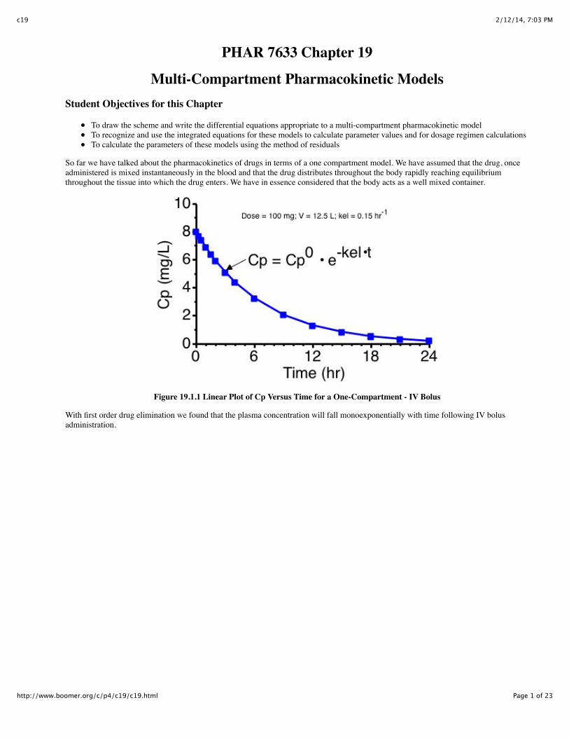
So far we have talked about the pharmacokinetics of drugs in terms of a one compartment model. We have assumed that the drug, onceadministered is mixed instantaneously in the blood and that the drug distributes throughout the body rapidly reaching equilibriumthroughout the tissue into which the drug enters. We have in essence considered that the body acts as a well mixed container.
Figure 19.1.1 Linear Plot of Cp Versus Time for a One-Compartment - IV Bolus
With first order drug elimination we found that the plasma concentration will fall monoexponentially with time following IV bolusadministration.

2/12/14, 7:03 PMc19
Page 2 of 23http://www.boomer.org/c/p4/c19/c19.html
Figure 19.1.2 Semi-Log Plot of Cp Versus Time
And the log of the plasma concentration will fall as a straight line.
Figure 19.1.3 Semi-Log Plot of Cp Versus Time. Two-Compartment - IV Bolus. Note Fast and Slow Processes
Commonly we find with real data, especially if we have a number of early data points, that the log Cp versus time plot is not a straightline. We see an initial early deviation from the straight line, followed by a log-linear phase. The initial phase is a more rapid drop inplasma concentration before settling into the log-linear fall in plasma concentration.
This suggests that the body is not behaving as a single well mixed compartment. There appears, mathematically, to be distributionbetween two (or more) compartments. That is we don't have instantaneous equilibrium between the drug in all the various tissues of thebody. In the next approximation we can consider that the body is behaving as two distinct compartments. These compartments can becalled the central compartment and the peripheral compartment. Exact anatomical assignment to these compartments is not alwayspossible. However, generally the rapidly perfused tissues often belong in the central compartment.
This page (http://www.boomer.org/c/p4/c19/c1901.html) was last modified: Wednesday 02 Oct 2013 at 12:03 PM
Material on this website should be used for Educational or Self-Study Purposes Only
Copyright © 2001-2014 David W. A. Bourne ([email protected])
TP

2/12/14, 7:03 PMc19
Page 3 of 23http://www.boomer.org/c/p4/c19/c19.html
PHAR 7633 Chapter 19
Multi-Compartment Pharmacokinetic Models
Intravenous Administration
Scheme or diagram
Figure 19.2.1 Two Compartment Pharmacokinetic Model
Clearance Model Equilibrium Model
Differential equation
The differential equation for drug in the central compartment following intravenous bolus administration is:-
Equation 19.2.1 Differential Equation for the Central Compartment
The kel • X1 term describes elimination of the drug from the central compartment, while the k12 • X1 and k21 • X2 terms describe thedistribution of drug between the central and peripheral compartments. Writing differential equations can be reviewed in Chapter 2.
Integrated equation
Integration of this equation (using Laplace transforms) leads to a biexponential equation for plasma concentration as a function of time,Equation 19.2.2
Equation 19.2.2 Integrated Equation for Plasma Concentration versus Time
Equation 19.2.3 Integrated Equation for Cp versus Time including k21 and V1
with α > β and

2/12/14, 7:03 PMc19
Page 4 of 23http://www.boomer.org/c/p4/c19/c19.html
Equation 19.2.4 Calculating values for A and B
The A, B, α, and β terms were derived from the micro-constants during the integration process. They are functions of the micro-constantk12, k21, kel and V1
Using the substitutions for the sum and product of α and β.
α + β = kel + k12 + k21
α • β = kel • k21
If we know the values of kel, k12 and k21 we can calculate α + β as well as α • β. Substituting these values into Equation 19.2.3 gives usvalues for α and β.
Equation 19.2.5 Converting from kel, k12 & k21 to α & β
Note, in this equation, α is calculated when '+' is used in the numerator and β is calculated when '-' is used in place of the '±'. Thus α isgreater than β.
Once we have values for α and β we can calculate values for A and B using Equation 19.2.4.
An example calculation (from the homework)
"A drug follows first order (i.e. linear) two compartment pharmacokinetics. After looking in the literature we find a number of parametervalues for this drug. These numbers represent the micro constants for this drug. In order that we can calculate the drug concentrationafter a single IV bolus dose these parameters need to be converted into values for the macro constants. The kel and V1 for this drug inthis patient (90.5 kg) are 0.192 hr-1 and 0.39 L/kg, respectively. The k12 and k21 values this drug are 1.86 and 1.68 hr-1, respectively.What is the plasma concentration of this drug 1.5 hours after a 500 mg, IV Bolus dose. In order to complete this calculation first calculatethe appropriate A, B, α and β values."
Since α + β = kel + k12 + k21 = 0.192 + 1.86 + 1.68 = 3.732
and
α x β = kel x k21 = 0.192 x 1.68 = 0.32256
Now:
α = [(a+b) + sqrt((a+b)2 - 4xaxb)]/2 = [3.732 + sqrt(3.7322 - 4x0.32256)]/2 = [3.732 + 3.5549]/2 = 3.643 hr-1
β = [3.732 - 3.5549]/2 = 0.08853 hr-1
A = Dose x (α - k21)/[V1 x (α - b)] = 500 x (3.643 - 1.68)/[90.5 x 0.39 x (3.643 - 0.08853)] = 500 x 1.963/[35.295 x 3.55447] = 7.824mg/L
B = Dose x (k21 - b)/[V1 x (α - b)] = 500 x (1.68 - 0.08853)/[35.295 x 3.55447] = 6.343 mg/L
The last step is
Cp = α x e(-α x t) + β x e(-β x t) = 7.824 x e(-3.643 x 1.5) + 6.343 x e(-0.08853 x 1.5) = 7.824 x 0.004234 + 6.343 x 0.8756 = 0.0331 + 5.5542= 5.59 mg/L

2/12/14, 7:03 PMc19
Page 5 of 23http://www.boomer.org/c/p4/c19/c19.html
Later in this chapter we will use equations for the reverse process of converting α, β, A and B into values for k12, k21, kel and V1.

2/12/14, 7:03 PMc19
Page 6 of 23http://www.boomer.org/c/p4/c19/c19.html
Calculator 19.2.1 Calculate A, B, α and β
Dose: 500
V1: 25
kel: 0.2
k21: 1.5
k12: 2.0
Calculate
A is:
α is:
B is:
β is:
This page (http://www.boomer.org/c/p4/c19/c1902.html) was last modified: Wednesday 02 Oct 2013 at 10:50 AM
Material on this website should be used for Educational or Self-Study Purposes Only
Copyright © 2001-2014 David W. A. Bourne ([email protected])
2/12/14, 7:03 PMc19
Page 7 of 23http://www.boomer.org/c/p4/c19/c19.html
PHAR 7633 Chapter 19
Multi-Compartment Pharmacokinetic Models
Parameter Determination
Method of residuals
Values for kel, k12, k12 and other parameters can be determined by first calculating A, B, α, and β. For this we can use the method ofresiduals (in a similar fashion to determining ka and kel for the one compartment model after oral administration). Starting with theequation for Cp.
Equation 19.3.1 Concentration versus time after an IV Bolus Dose, Two Compartment Model
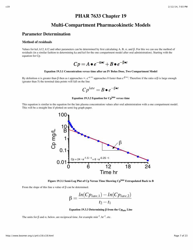
By definition α is greater than β then as t approaches ∞, e-α • t approaches 0 faster than e-β • t. Therefore if the ratio α/β is large enough(greater than 5) the terminal data points will fall on the line
Equation 19.3.2 Equation for Cplate versus time
This equation is similar to the equation for the late plasma concentration values after oral administration with a one compartment model.This will be a straight line if plotted on semi-log graph paper.
Figure 19.3.1 Semi-Log Plot of Cp Versus Time Showing Cplate Extrapolated Back to B
From the slope of this line a value of β can be determined.
Equation 19.3.3 Determining β from the Cplate Line
The units for β and α, below, are reciprocal time, for example min-1, hr-1, etc.

2/12/14, 7:03 PMc19
Page 8 of 23http://www.boomer.org/c/p4/c19/c19.html
Biological half-life or Terminal half-life
The t1/2 calculated as 0.693/β is often called the biological half-life or terminal half-life. It is the half-life describing the terminalelimination of the drug from plasma. [For the one compartment model the biological half-life was equal to 0.693/kel].
The difference between the Cplate values (red line) at early times and the actual data at early times is again termed the 'residual'
Equation 19.3.4 Equation for Residual versus time
Figure 19.3.2 Semi-Log Plot of Cp Versus Time Showing Residual Line and Cplate Line
Click on the figure to view as an interactive graph or a Interactive graph as a Linear Plot
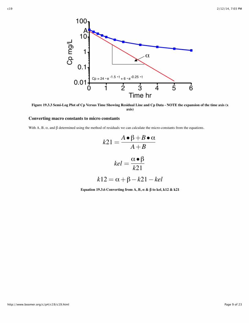
The slope of the residual line (green line) will provide the value of α and A can be estimated as the intercept of the concentration axis (y-axis). A more accurate value for the α value can be determined by expanding the scale on the time axis (Figure 19.3.3). Don't forget touse the new time values when calculating α from the equation
Equation 19.3.5 Determining α from the Residual Line
2/12/14, 7:03 PMc19
Page 9 of 23http://www.boomer.org/c/p4/c19/c19.html
Figure 19.3.3 Semi-Log Plot of Cp Versus Time Showing Residual Line and Cp Data - NOTE the expansion of the time axis (xaxis)
Converting macro constants to micro constants
With A, B, α, and β determined using the method of residuals we can calculate the micro-constants from the equations.
Equation 19.3.6 Converting from A, B, α & β to kel, k12 & k21
2/12/14, 7:03 PMc19
Page 10 of 23http://www.boomer.org/c/p4/c19/c19.html
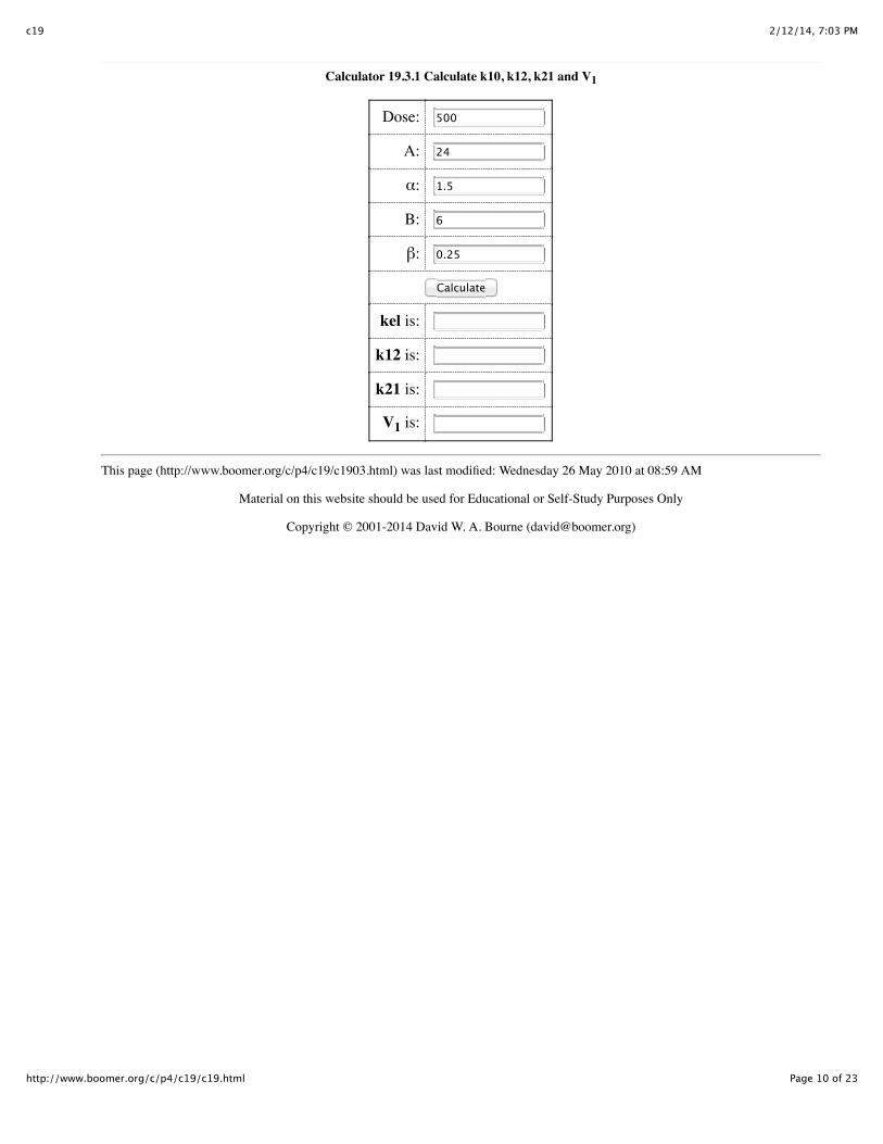
Calculator 19.3.1 Calculate k10, k12, k21 and V1
Dose: 500
A: 24
α: 1.5
B: 6
β: 0.25
Calculate
kel is:
k12 is:
k21 is:
V1 is:
This page (http://www.boomer.org/c/p4/c19/c1903.html) was last modified: Wednesday 26 May 2010 at 08:59 AM
Material on this website should be used for Educational or Self-Study Purposes Only
Copyright © 2001-2014 David W. A. Bourne ([email protected])

2/12/14, 7:03 PMc19
Page 11 of 23http://www.boomer.org/c/p4/c19/c19.html
PHAR 7633 Chapter 19
Multi-Compartment Pharmacokinetic Models
Effect of k12 and k21 on Drug Concentration versus Time
Changing the Ratio of k12 to k21
Figure 19.4.1 Plot of Cp versus Time Showing the Effect of Different k12/21 Ratio Values
Click on the figure to view as an interactive graph or a Interactive graph as a Semi-log Plot
From the k12 and k21 values we can assess the extent of distribution of drug into the peripheral compartment. The higher the ratiok12/k21 the greater the distribution of drug into the peripheral compartment. The larger the individual values of k12 and k21 the faster isthe transfer between the central and peripheral compartments and the more the body behaves as a single compartment.
As the ratio increases the distribution phase is more pronounced. Conversely with the ratio 1/4 there is very little distribution phase. Alsonote that the β value or the slope of the terminal phase is changing even though the kel is fixed at 0.2 hr-1.
Changing the Magnitude of k12 and k21 with the Same Ratio
With faster and faster distribution the initial drop in plasma concentration becomes quite rapid. If you were sampling every 30 minutes,the initial phase would be missed. The data would look just like a one compartment model. Redrawing the slow plot with k12/k21(0.5/0.25) over 24 hours and gives a plot that is definitely still biexponential.

2/12/14, 7:03 PMc19
Page 12 of 23http://www.boomer.org/c/p4/c19/c19.html
Figure 19.4.2 Plot of Cp versus Time Showing the Effect of Different k12/21 Magnitudes
Click on the figure to view as an interactive graph or a Interactive graph as a Semi-log Plot
Simulate other concentration versus time curves after IV bolus administration with the two compartment pharmacokinetic model using
macro constants (A, B, α and β)
Linear plot - Semi-log plot
or micro constants (kel, k12, k21, and V1)
Linear plot - Semi-log plot
This page (http://www.boomer.org/c/p4/c19/c1904.html) was last modified: Wednesday 26 May 2010 at 08:59 AM
Material on this website should be used for Educational or Self-Study Purposes Only
Copyright © 2001-2014 David W. A. Bourne ([email protected])
2/12/14, 7:03 PMc19
Page 13 of 23http://www.boomer.org/c/p4/c19/c19.html
PHAR 7633 Chapter 19
Multi-Compartment Pharmacokinetic Models
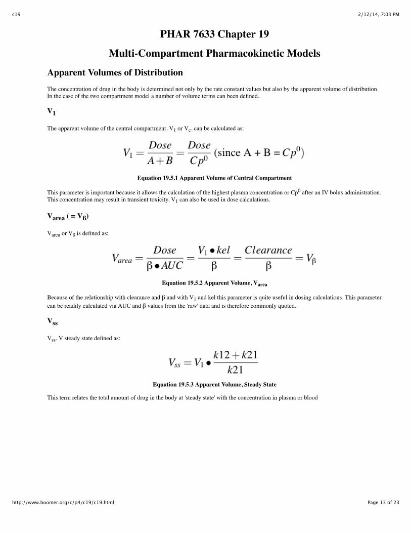
Apparent Volumes of DistributionThe concentration of drug in the body is determined not only by the rate constant values but also by the apparent volume of distribution.In the case of the two compartment model a number of volume terms can been defined.
V1
The apparent volume of the central compartment, V1 or Vc, can be calculated as:
Equation 19.5.1 Apparent Volume of Central Compartment
This parameter is important because it allows the calculation of the highest plasma concentration or Cp0 after an IV bolus administration.This concentration may result in transient toxicity. V1 can also be used in dose calculations.
Varea ( = Vß)
Varea or Vß is defined as:
Equation 19.5.2 Apparent Volume, Varea
Because of the relationship with clearance and β and with V1 and kel this parameter is quite useful in dosing calculations. This parametercan be readily calculated via AUC and β values from the 'raw' data and is therefore commonly quoted.
Vss
Vss, V steady state defined as:
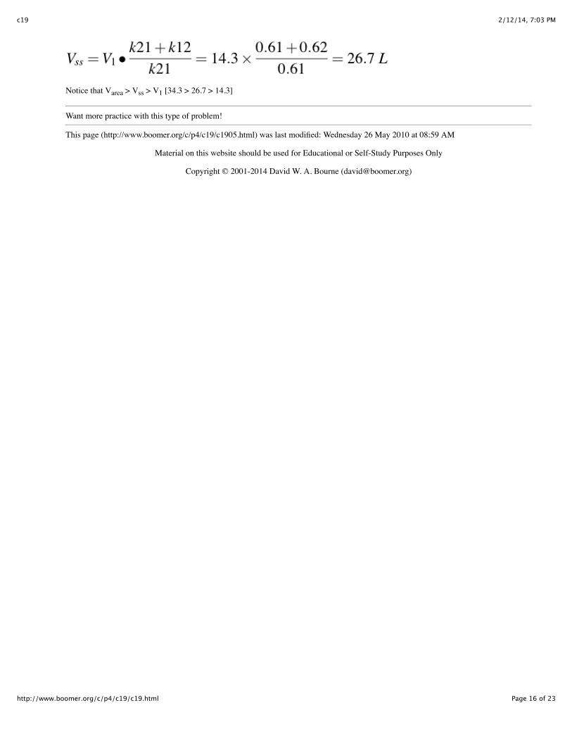
Equation 19.5.3 Apparent Volume, Steady State
This term relates the total amount of drug in the body at 'steady state' with the concentration in plasma or blood

2/12/14, 7:03 PMc19
Page 14 of 23http://www.boomer.org/c/p4/c19/c19.html
Figure 19.5.1 Plot of X1 (Plasma) and X2 (Tissue) Compartment Concentrations, Showing 'Steady State' with Both Lines Parallel
The relationship between volume terms is that:
Varea > Vss > V1
And for a one compartment model the values for all these parameters are equal.
Example Calculation
As an example we can look at the data in the table below.
Table 19.5.1 Two Compartment Pharmacokinetics
Time (hr) Concentration (mg/L) Cplate (mg/L) Residual (mg/L)
0.5 20.6 8.8 11.8
1 13.4 7.8 5.6
2 7.3 6.1 1.2
3 5.0 4.7 0.3
4 3.7 3.7 -
6 2.2
8 1.4
10 0.82
12 0.50

2/12/14, 7:03 PMc19
Page 15 of 23http://www.boomer.org/c/p4/c19/c19.html
Figure 19.5.2 Plot of Cp versus Time Illustrating the Method of Residuals
The first two columns are the time and plasma concentration which may be collected after IV bolus administration of 500 mg of drug.These data are plotted (n) in Figure 19.5.2 above. At longer times, after 4 hours, out to 12 hours the data appears to follow a straight lineon semi- log graph paper. Since α > β this terminal line is described by B • e-β • t.
Following it back to t = 0 gives B = 10 mg/L. From the slope of the line β = 0.25 hr-1. Cplate values at early times are shown in column 3and the residual in column 4. The residual values are plotted (o) also giving a value of A = 25 mg/L and α = 1.51 hr-1 Note that α/β = 6,thus these values should be fairly accurate.
B = 10 mg/L, β = (ln 10 - ln 0.5)/12 = 2.996/12 = 0.25 hr-1
A = 25 mg/L, α = (ln 25 - ln 0.27)/3 = 4.528/3 = 1.51 hr-1
Therefore Cp = 25 • e-1.51 • t + 10 • e-0.25 • t
We can now calculate the micro-constants.
The AUC by the trapezoidal rule + Cplast/β = 56.3 + 2.0 = 58.3 mg.hr.L-1, [Note the use of β] thus
2/12/14, 7:03 PMc19
Page 16 of 23http://www.boomer.org/c/p4/c19/c19.html
Notice that Varea > Vss > V1 [34.3 > 26.7 > 14.3]
Want more practice with this type of problem!
This page (http://www.boomer.org/c/p4/c19/c1905.html) was last modified: Wednesday 26 May 2010 at 08:59 AM
Material on this website should be used for Educational or Self-Study Purposes Only
Copyright © 2001-2014 David W. A. Bourne ([email protected])
2/12/14, 7:03 PMc19
Page 17 of 23http://www.boomer.org/c/p4/c19/c19.html
PHAR 7633 Chapter 19
Multi-Compartment Pharmacokinetic Models
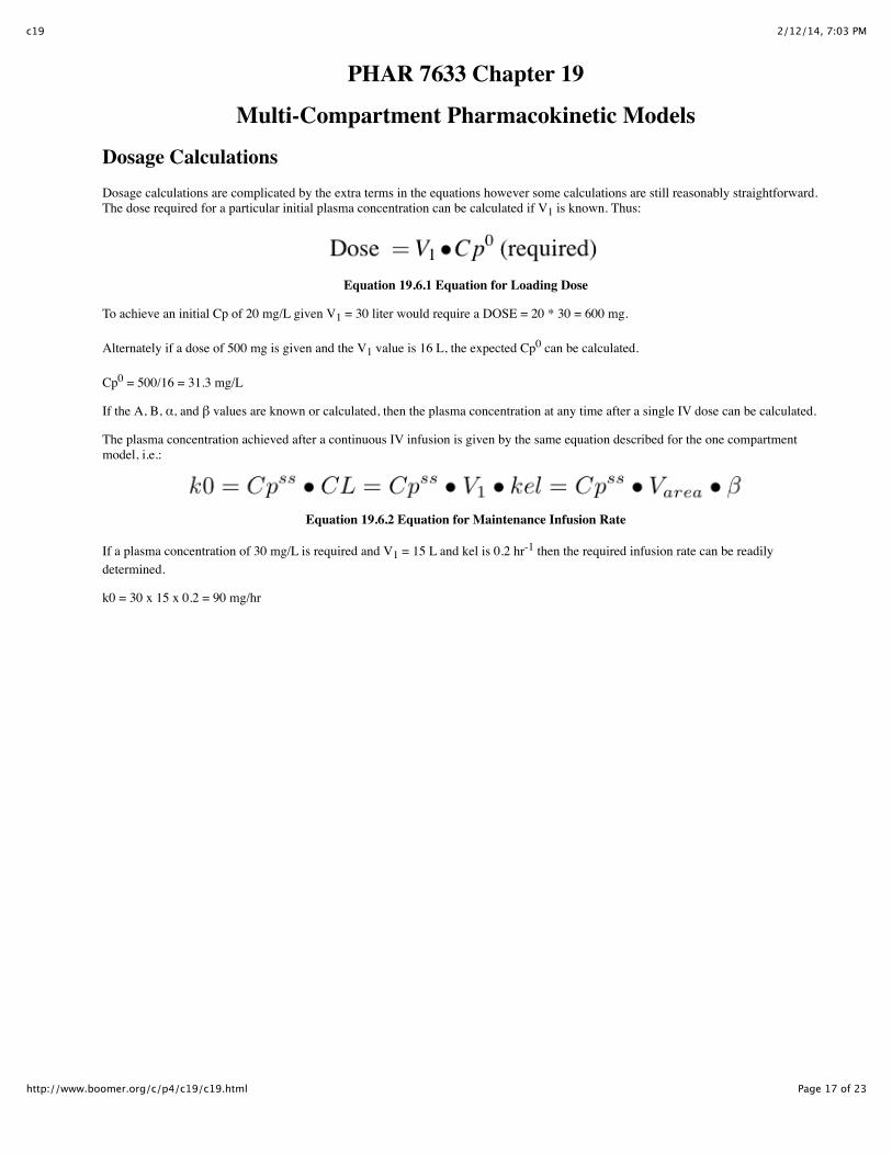
Dosage CalculationsDosage calculations are complicated by the extra terms in the equations however some calculations are still reasonably straightforward.The dose required for a particular initial plasma concentration can be calculated if V1 is known. Thus:
Equation 19.6.1 Equation for Loading Dose
To achieve an initial Cp of 20 mg/L given V1 = 30 liter would require a DOSE = 20 * 30 = 600 mg.
Alternately if a dose of 500 mg is given and the V1 value is 16 L, the expected Cp0 can be calculated.
Cp0 = 500/16 = 31.3 mg/L
If the A, B, α, and β values are known or calculated, then the plasma concentration at any time after a single IV dose can be calculated.
The plasma concentration achieved after a continuous IV infusion is given by the same equation described for the one compartmentmodel, i.e.:
Equation 19.6.2 Equation for Maintenance Infusion Rate
If a plasma concentration of 30 mg/L is required and V1 = 15 L and kel is 0.2 hr-1 then the required infusion rate can be readilydetermined.
k0 = 30 x 15 x 0.2 = 90 mg/hr

2/12/14, 7:03 PMc19
Page 18 of 23http://www.boomer.org/c/p4/c19/c19.html
Figure 19.6.1 Linear Plot of Cp Versus Time With IV Bolus and Infusion
Click on the figure to view as an interactive graph or a Interactive graph as a Semi-log Plot
Since the time to reach the steady state concentration is controlled by the β value this could mean a slow approach to the desired value,thus an IV bolus loading dose may be useful. Unfortunately this calculation is not straight forward as you will see if you explore theapplet.
With V1 = 15 L, kel = 0.2 hr-1, and required Cp = 30 mg/L
Bolus DOSE = 15 x 30 = 450 mg and
Infusion Rate = k0 = 30 x 15 x 0.2 = 90 mg/hr
Figure 19.6.2 Linear Plot after an IV Infusion and a Higher or Lower Bolus Dose
As you can see (Figure 19.6.1 and 19.6.2 above) this gives quite a dip in the Cp versus time curve.
With Bolus DOSEs, either 600 or 300 mg (shown in Figure 19.6.2) the curves may or may not be better depending on the therapeuticrange of the drug.

2/12/14, 7:03 PMc19
Page 19 of 23http://www.boomer.org/c/p4/c19/c19.html
Figure 19.6.3 Linear Plot of Cp versus Time With Fast and Slow Infusion
Click on the figure to view as an interactive graph or a Interactive graph as a Semi-log Plot
Another alternative is to give a fast infusion followed by the maintenance infusion. Here 1200 mg was given over 4 hours (at 300 mg/hr)before switching to the slower 90 mg/hr maintenance rate.
Try a dosing problem with a drug following a two compartment pharmacokinetic model.
This page (http://www.boomer.org/c/p4/c19/c1906.html) was last modified: Wednesday 26 May 2010 at 08:59 AM
Material on this website should be used for Educational or Self-Study Purposes Only
Copyright © 2001-2014 David W. A. Bourne ([email protected])

2/12/14, 7:03 PMc19
Page 20 of 23http://www.boomer.org/c/p4/c19/c19.html
PHAR 7633 Chapter 19
Multi-Compartment Pharmacokinetic Models
Oral AdministrationFollowing oral administration of a drug with two compartment characteristics, Cp is described by an equation with three exponentialterms.
Diagram 19.7.1 Scheme for Oral Two-Compartment Pharmacokinetic Model
The model is shown in Diagram 19.7.1.
Equation 19.7.1 Differential Equation for Drug Amount in the Body after Oral Administration
Differential equation
Equation 19.7.2 Integrated Equation for Drug Amount in the Body after Oral Administration
where A + B + C = 0

2/12/14, 7:03 PMc19
Page 21 of 23http://www.boomer.org/c/p4/c19/c19.html
Figure 19.7.1 Semi-Log Plot Showing Pronounced Distribution
Figure 19.7.2 Semi-Log Plot Without Distribution Phase Evident

2/12/14, 7:03 PMc19
Page 22 of 23http://www.boomer.org/c/p4/c19/c19.html
Bioavailability
Bioavailability calculations are the same as for the one compartment model, i.e., by comparison of AUC or U∞. These apply for anylinear system. Also if α, β, and ka are sufficiently separated the method of residuals can be applied (twice) to determine values for thesethree parameters.
Average Plasma Concentration
The average plasma concentration equation can also be used to calculate appropriate dosing regimens. For example if an average plasmaconcentration of 20 mg/L is required and V1 = 15 L, kel = 0.15 hr-1, F = 0.9 and a dosing interval of 12 hours is to be used then therequired dose can be calculated from the equation for Cpaverage.
Equation 19.7.3 Equation for Average Plasma Concentration
The required dose can be calculated using Equation 19.7.3 and the data provided. Thus
2/12/14, 7:03 PMc19
Page 23 of 23http://www.boomer.org/c/p4/c19/c19.html
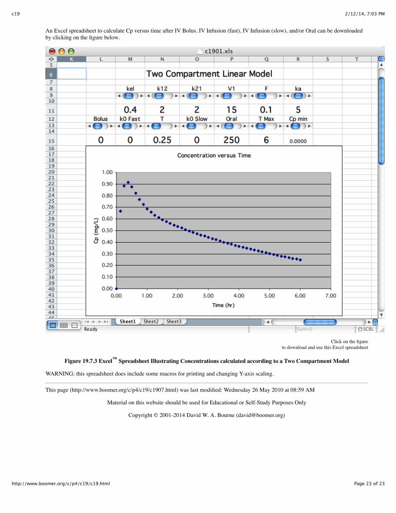
An Excel spreadsheet to calculate Cp versus time after IV Bolus, IV Infusion (fast), IV Infusion (slow), and/or Oral can be downloadedby clicking on the figure below.
Click on the figureto download and use this Excel spreadsheet
Figure 19.7.3 Excel™ Spreadsheet Illustrating Concentrations calculated according to a Two Compartment Model
WARNING; this spreadsheet does include some macros for printing and changing Y-axis scaling.
This page (http://www.boomer.org/c/p4/c19/c1907.html) was last modified: Wednesday 26 May 2010 at 08:59 AM
Material on this website should be used for Educational or Self-Study Purposes Only
Copyright © 2001-2014 David W. A. Bourne ([email protected])
Top Related