


Languages
Pages
Legal


Package ‘emplik’August 17, 2018
Maintainer Mai Zhou <[email protected]>
Version 1.0-4.3
Depends R (>= 3.0)
Imports quantreg, stats
Suggests KMsurv, boot
Author Mai Zhou. (Art Owen for el.test(). Yifan Yang for C code.)
Description Empirical likelihood ratio tests for means/quantiles/hazardsfrom possibly censored and/or truncated data. Now does regression too.This version contains some C code.
Title Empirical Likelihood Ratio for Censored/Truncated Data
License GPL (>= 2)
URL http://www.ms.uky.edu/~mai/EmpLik.html
NeedsCompilation yes
Repository CRAN
Date/Publication 2018-08-17 20:50:54 UTC
R topics documented:BJnoint . . . . . . . . . . . . . . . . . . . . . . . . . . . . . . . . . . . . . . . . . . . 2bjtest . . . . . . . . . . . . . . . . . . . . . . . . . . . . . . . . . . . . . . . . . . . . . 3bjtest1d . . . . . . . . . . . . . . . . . . . . . . . . . . . . . . . . . . . . . . . . . . . 5bjtestII . . . . . . . . . . . . . . . . . . . . . . . . . . . . . . . . . . . . . . . . . . . . 6el.cen.EM . . . . . . . . . . . . . . . . . . . . . . . . . . . . . . . . . . . . . . . . . . 8el.cen.EM2 . . . . . . . . . . . . . . . . . . . . . . . . . . . . . . . . . . . . . . . . . 10el.cen.test . . . . . . . . . . . . . . . . . . . . . . . . . . . . . . . . . . . . . . . . . . 14el.ltrc.EM . . . . . . . . . . . . . . . . . . . . . . . . . . . . . . . . . . . . . . . . . . 16el.test . . . . . . . . . . . . . . . . . . . . . . . . . . . . . . . . . . . . . . . . . . . . 18el.test.wt . . . . . . . . . . . . . . . . . . . . . . . . . . . . . . . . . . . . . . . . . . . 20el.test.wt2 . . . . . . . . . . . . . . . . . . . . . . . . . . . . . . . . . . . . . . . . . . 21el.trun.test . . . . . . . . . . . . . . . . . . . . . . . . . . . . . . . . . . . . . . . . . . 23emplikH.disc . . . . . . . . . . . . . . . . . . . . . . . . . . . . . . . . . . . . . . . . 25
1

2 BJnoint
emplikH.disc2 . . . . . . . . . . . . . . . . . . . . . . . . . . . . . . . . . . . . . . . . 27emplikH1.test . . . . . . . . . . . . . . . . . . . . . . . . . . . . . . . . . . . . . . . . 29emplikH2.test . . . . . . . . . . . . . . . . . . . . . . . . . . . . . . . . . . . . . . . . 31emplikHs.disc2 . . . . . . . . . . . . . . . . . . . . . . . . . . . . . . . . . . . . . . . 33emplikHs.test2 . . . . . . . . . . . . . . . . . . . . . . . . . . . . . . . . . . . . . . . 35findUL . . . . . . . . . . . . . . . . . . . . . . . . . . . . . . . . . . . . . . . . . . . . 38findUL2 . . . . . . . . . . . . . . . . . . . . . . . . . . . . . . . . . . . . . . . . . . . 40findULold . . . . . . . . . . . . . . . . . . . . . . . . . . . . . . . . . . . . . . . . . . 42myeloma . . . . . . . . . . . . . . . . . . . . . . . . . . . . . . . . . . . . . . . . . . 43RankRegTest . . . . . . . . . . . . . . . . . . . . . . . . . . . . . . . . . . . . . . . . 44RankRegTestH . . . . . . . . . . . . . . . . . . . . . . . . . . . . . . . . . . . . . . . 46ROCnp . . . . . . . . . . . . . . . . . . . . . . . . . . . . . . . . . . . . . . . . . . . 48ROCnp2 . . . . . . . . . . . . . . . . . . . . . . . . . . . . . . . . . . . . . . . . . . . 49smallcell . . . . . . . . . . . . . . . . . . . . . . . . . . . . . . . . . . . . . . . . . . . 51WRegEst . . . . . . . . . . . . . . . . . . . . . . . . . . . . . . . . . . . . . . . . . . 52WRegTest . . . . . . . . . . . . . . . . . . . . . . . . . . . . . . . . . . . . . . . . . . 53
Index 55
BJnoint The Buckley-James censored regression estimator
Description
Compute the Buckley-James estimator in the regression model
yi = βxi + εi
with right censored yi. Iteration method.
Usage
BJnoint(x, y, delta, beta0 = NA, maxiter=30, error = 0.00001)
Arguments
x a matrix or vector containing the covariate, one row per observation.
y a numeric vector of length N, censored responses.
delta a vector of length N, delta=0/1 for censored/uncensored.
beta0 an optional vector for starting value of iteration.
maxiter an optional integer to control iterations.
error an optional positive value to control iterations.
bjtest 3
Details
This function compute the Buckley-James estimator when your model do not have an interceptterm. Of course, if you include a column of 1’s in the x matrix, it is also OK with this function andit is equivalent to having an intercept term. If your model do have an intercept term, then you couldalso (probably should) use the function bj( ) in the Design library. It should be more refined thanBJnoint in the stopping rule for the iterations.
This function is included here mainly to produce the estimator value that may provide some usefulinformation with the function bjtest( ). For example you may want to test a beta value near theBuckley-James estimator.
Value
A list with the following components:
beta the Buckley-James estimator.
iteration number of iterations performed.
Author(s)
Mai Zhou.
References
Buckley, J. and James, I. (1979). Linear regression with censored data. Biometrika, 66 429-36.
Examples
x <- matrix(c(rnorm(50,mean=1), rnorm(50,mean=2)), ncol=2,nrow=50)## Suppose now we wish to test Ho: 2mu(1)-mu(2)=0, theny <- 2*x[,1]-x[,2]xx <- c(28,-44,29,30,26,27,22,23,33,16,24,29,24,40,21,31,34,-2,25,19)
bjtest Test the Buckley-James estimator by Empirical Likelihood
Description
Use the empirical likelihood ratio and Wilks theorem to test if the regression coefficient is equal tobeta.
The log empirical likelihood been maximized is∑d=1
log ∆F (ei) +∑d=0
log[1 − F (ei)];
where ei are the residuals.

4 bjtest
Usage
bjtest(y, d, x, beta)
Arguments
y a vector of length N, containing the censored responses.
d a vector (length N) of either 1’s or 0’s. d=1 means y is uncensored; d=0 meansy is right censored.
x a matrix of size N by q.
beta a vector of length q. The value of the regression coefficient to be tested in themodel yi = βxi + εi
Details
The above likelihood should be understood as the likelihood of the error term, so in the regressionmodel the error epsilon should be iid.
This version can handle the model where beta is a vector (of length q).
The estimation equations used when maximize the empirical likelihood is
0 =∑
di∆F (ei)(x ·m[, i])/(nwi)
which was described in detail in the reference below.
Value
A list with the following components:
"-2LLR" the -2 loglikelihood ratio; have approximate chisq distribution under Ho.
logel2 the log empirical likelihood, under estimating equation.
logel the log empirical likelihood of the Kaplan-Meier of e’s.
prob the probabilities that max the empirical likelihood under estimating equation.
Author(s)
Mai Zhou.
References
Buckley, J. and James, I. (1979). Linear regression with censored data. Biometrika, 66 429-36.
Zhou, M. and Li, G. (2008). Empirical likelihood analysis of the Buckley-James estimator. Journalof Multivariate Analysis 99, 649-664.
Zhou, M. (2016) Empirical Likelihood Method in Survival Analysis. CRC Press.
Examples
xx <- c(28,-44,29,30,26,27,22,23,33,16,24,29,24,40,21,31,34,-2,25,19)

bjtest1d 5
bjtest1d Test the Buckley-James estimator by Empirical Likelihood, 1-dim only
Description
Use the empirical likelihood ratio and Wilks theorem to test if the regression coefficient is equal tobeta. For 1-dim beta only.
The log empirical likelihood been maximized is∑d=1
log ∆F (ei) +∑d=0
log[1 − F (ei)].
Usage
bjtest1d(y, d, x, beta)
Arguments
y a vector of length N, containing the censored responses.
d a vector of either 1’s or 0’s. d=1 means y is uncensored. d=0 means y is rightcensored.
x a vector of length N, covariate.
beta a number. the regression coefficient to be tested in the model y = x beta + epsilon
Details
In the above likelihood, ei = yi − x ∗ beta is the residuals.
Similar to bjtest( ), but only for 1-dim beta.
Value
A list with the following components:
"-2LLR" the -2 loglikelihood ratio; have approximate chi square distribution under Ho.
logel2 the log empirical likelihood, under estimating equation.
logel the log empirical likelihood of the Kaplan-Meier of e’s.
prob the probabilities that max the empirical likelihood under estimating equationconstraint.
Author(s)
Mai Zhou.

6 bjtestII
References
Buckley, J. and James, I. (1979). Linear regression with censored data. Biometrika, 66 429-36.
Owen, A. (1990). Empirical likelihood ratio confidence regions. Ann. Statist. 18 90-120.
Zhou, M. and Li, G. (2008). Empirical likelihood analysis of the Buckley-James estimator. Journalof Multivariate Analysis. 649-664.
Examples
xx <- c(28,-44,29,30,26,27,22,23,33,16,24,29,24,40,21,31,34,-2,25,19)
bjtestII Alternative test of the Buckley-James estimator by Empirical Likeli-hood
Description
Use the empirical likelihood ratio (alternative form) and Wilks theorem to test if the regressioncoefficient is equal to beta, based on the estimating equations.
The log empirical likelihood been maximized is
n∑j=1
log pj ;∑
pj = 1
where the probability pj is for the jth martingale differences of the estimating equations.
Usage
bjtestII(y, d, x, beta)
Arguments
y a vector of length N, containing the censored responses.
d a vector of length N. Either 1’s or 0’s. d=1 means y is uncensored; d=0 means yis right censored.
x a matrix of size N by q.
beta a vector of length q. The value of the regression coefficient to be tested in themodel Yi = βxi + εi
bjtestII 7
Details
The above likelihood should be understood as the likelihood of the martingale difference terms. Forthe definition of the Buckley-James martingale or estimating equation, please see the (2015) bookin the reference list.
The estimation equations used when maximize the empirical likelihood is
0 =∑
di∆F (ei)(x ·m[, i])/(nwi)
where ei is the residuals, other details are described in the reference book of 2015 below.
The final test is carried out by el.test. So the output is similar to the output of el.test.
Value
A list with the following components:
"-2LLR" the -2 loglikelihood ratio; have approximate chisq distribution under Ho.
logel2 the log empirical likelihood, under estimating equation.
logel the log empirical likelihood of the Kaplan-Meier of e’s.
prob the probabilities that max the empirical likelihood under estimating equation.
Author(s)
Mai Zhou.
References
Zhou, M. (2016) Empirical Likelihood Methods in Survival Analysis. CRC Press.
Buckley, J. and James, I. (1979). Linear regression with censored data. Biometrika, 66 429-36.
Zhou, M. and Li, G. (2008). Empirical likelihood analysis of the Buckley-James estimator. Journalof Multivariate Analysis, 99, 649–664.
Zhu, H. (2007) Smoothed Empirical Likelihood for Quantiles and Some Variations/Extension ofEmpirical Likelihood for Buckley-James Estimator, Ph.D. dissertation, University of Kentucky.
Examples
data(myeloma)bjtestII(y=myeloma[,1], d=myeloma[,2], x=cbind(1, myeloma[,3]), beta=c(37, -3.4))

8 el.cen.EM
el.cen.EM Empirical likelihood ratio for mean with right, left or doubly censoreddata, by EM algorithm
Description
This program uses EM algorithm to compute the maximized (wrt pi) empirical log likelihood func-tion for right, left or doubly censored data with the MEAN constraint:∑
di=1
pif(xi) =
∫f(t)dF (t) = µ.
Where pi = ∆F (xi) is a probability, di is the censoring indicator, 1(uncensored), 0(right censored),2(left censored). It also returns those pi.
The empirical log likelihood been maximized is∑di=1
log ∆F (xi) +∑di=0
log[1 − F (xi)] +∑di=2
logF (xi).
Usage
el.cen.EM(x,d,wt=rep(1,length(d)),fun=function(t){t},mu,maxit=25,error=1e-9,...)
Arguments
x a vector containing the observed survival times.
d a vector containing the censoring indicators, 1-uncensored; 0-right censored;2-left censored.
wt a weight vector (case weight). positive. same length as d
fun a left continuous (weight) function used to calculate the mean as in H0. fun(t)must be able to take a vector input t. Default to the identity function f(t) = t.
mu a real number used in the constraint, the mean value of f(X).
maxit an optional integer, used to control maximum number of iterations.
error an optional positive real number specifying the tolerance of iteration error. Thisis the bound of the L1 norm of the difference of two successive weights.
... additional arguments, if any, to pass to fun.
Details
This implementation is all in R and have several for-loops in it. A faster version would use C to dothe for-loop part. But this version seems faster enough and is easier to port to Splus.
We return the log likelihood all the time. Sometimes, (for right censored and no censor case) wealso return the -2 log likelihood ratio. In other cases, you have to plot a curve with many values ofthe parameter, mu, to find out where is the place the log likelihood becomes maximum. And from
el.cen.EM 9
there you can get -2 log likelihood ratio between the maximum location and your current parameterin Ho.
In order to get a proper distribution as NPMLE, we automatically change the d for the largestobservation to 1 (even if it is right censored), similar for the left censored, smallest observation. µis a given constant. When the given constants µ is too far away from the NPMLE, there will beno distribution satisfy the constraint. In this case the computation will stop. The -2 Log empiricallikelihood ratio should be infinite.
The constant mu must be inside (min f(xi),max f(xi)) for the computation to continue. It is alwaystrue that the NPMLE values are feasible. So when the computation stops, try move the mu closer tothe NPMLE — ∑
di=1
p0i f(xi)
p0i taken to be the jumps of the NPMLE of CDF. Or use a different fun.
Difference to the function el.cen.EM2: here duplicate (input) observations are collapsed (withweight 2, 3, ... etc.) but those will stay separate by default in the el.cen.EM2. This will lead to adifferent loglik value. But the -2LLR value should be same in either version.
Value
A list with the following components:
loglik the maximized empirical log likelihood under the constraint.
times locations of CDF that have positive mass.
prob the jump size of CDF at those locations.
"-2LLR" If available, it is Minus two times the Empirical Log Likelihood Ratio. Shouldbe approximately chi-square distributed under Ho.
Pval The P-value of the test, using chi-square approximation.
lam The Lagrange multiplier. Added 5/2007.
Author(s)
Mai Zhou
References
Zhou, M. (2005). Empirical likelihood ratio with arbitrary censored/truncated data by EM algo-rithm. Journal of Computational and Graphical Statistics, 643-656.
Murphy, S. and van der Vaart (1997) Semiparametric likelihood ratio inference. Ann. Statist. 25,1471-1509.
Examples
## example with tied observationsx <- c(1, 1.5, 2, 3, 4, 5, 6, 5, 4, 1, 2, 4.5)d <- c(1, 1, 0, 1, 0, 1, 1, 1, 1, 0, 0, 1)el.cen.EM(x,d,mu=3.5)## we should get "-2LLR" = 1.2466....

10 el.cen.EM2
myfun5 <- function(x, theta, eps) {u <- (x-theta)*sqrt(5)/epsINDE <- (u < sqrt(5)) & (u > -sqrt(5))u[u >= sqrt(5)] <- 0u[u <= -sqrt(5)] <- 1y <- 0.5 - (u - (u)^3/15)*3/(4*sqrt(5))u[ INDE ] <- y[ INDE ]return(u)}el.cen.EM(x, d, fun=myfun5, mu=0.5, theta=3.5, eps=0.1)## example of using wt in the input. Since the x-vector contain## two 5 (both d=1), and two 2(both d=0), we can also doxx <- c(1, 1.5, 2, 3, 4, 5, 6, 4, 1, 4.5)dd <- c(1, 1, 0, 1, 0, 1, 1, 1, 0, 1)wt <- c(1, 1, 2, 1, 1, 2, 1, 1, 1, 1)el.cen.EM(x=xx, d=dd, wt=wt, mu=3.5)## this should be the same as the first example.
el.cen.EM2 Empirical likelihood ratio test for a vector of means with right, left ordoubly censored data, by EM algorithm
Description
This function is similar to el.cen.EM(), but for multiple constraints. In the input there is a vectorof observations x = (x1, · · · , xn) and a function fun. The function fun should return the (n by k)matrix
(f1(x), f2(x), · · · , fk(x)).
Also, the ordering of the observations, when consider censoring or redistributing-to-the-right, isaccording to the value of x, not fun(x). So the probability distribution is for values x. This programuses EM algorithm to maximize (wrt pi) empirical log likelihood function for right, left or doublycensored data with the MEAN constraint:
j = 1, 2, · · · , k∑di=1
pifj(xi) =
∫fj(t)dF (t) = µj .
Where pi = ∆F (xi) is a probability, di is the censoring indicator, 1(uncensored), 0(right censored),2(left censored). It also returns those pi. The log likelihood function is defined as∑
di=1
log ∆F (xi) +∑di=2
logF (xi) +∑di=0
log[1 − F (xi)] .
Usage
el.cen.EM2(x,d,xc=1:length(x),fun,mu,maxit=25,error=1e-9,...)

el.cen.EM2 11
Arguments
x a vector containing the observed survival times.
d a vector containing the censoring indicators, 1-uncensored; 0-right censored;2-left censored.
xc an optional vector of collapsing control values. If xc[i] xc[j] have different val-ues then (x[i], d[i]), (x[j], d[j]) will not merge into one observation with weighttwo, even if they are identical. Default is not to merge.
fun a left continuous (weight) function that returns a matrix. The columns (=k) ofthe matrix is used to calculate the means and will be tested in H0. fun(t) mustbe able to take a vector input t.
mu a vector of length k. Used in the constraint, as the mean of f(X).
maxit an optional integer, used to control maximum number of iterations.
error an optional positive real number specifying the tolerance of iteration error. Thisis the bound of the L1 norm of the difference of two successive weights.
... additional inputs to pass to fun().
Details
This implementation is all in R and have several for-loops in it. A faster version would use C to dothe for-loop part. (but this version is easier to port to Splus, and seems faster enough).
We return the log likelihood all the time. Sometimes, (for right censored and no censor case) wealso return the -2 log likelihood ratio. In other cases, you have to plot a curve with many values ofthe parameter, mu, to find out where the log likelihood becomes maximum. And from there youcan get -2 log likelihood ratio between the maximum location and your current parameter in Ho.
In order to get a proper distribution as NPMLE, we automatically change the d for the largestobservation to 1 (even if it is right censored), similar for the left censored, smallest observation.µ is a given constant vector. When the given constants µ is too far away from the NPMLE, therewill be no distribution satisfy the constraint. In this case the computation will stop. The -2 Logempirical likelihood ratio should be infinite.
The constant vector mu must be inside (min f(xi),max f(xi)) for the computation to continue. Itis always true that the NPMLE values are feasible. So when the computation stops, try move the mucloser to the NPMLE —
µ̂j =∑di=1
p0i fj(xi)
where p0i taken to be the jumps of the NPMLE of CDF. Or use a different fun.
Difference to the function el.cen.EM: due to the introduction of input xc here in this function,the output loglik may be different compared to the function el.cen.EM due to not collapsing ofduplicated input survival values. The -2LLR should be the same from both functions.
Value
A list with the following components:
loglik the maximized empirical log likelihood under the constraints.
times locations of CDF that have positive mass.

12 el.cen.EM2
prob the jump size of CDF at those locations.
"-2LLR" If available, it is Minus two times the Empirical Log Likelihood Ratio. Shouldbe approx. chi-square distributed under Ho.
Pval If available, the P-value of the test, using chi-square approximation.
lam the Lagrange multiplier in the final EM step. (the M-step)
Author(s)
Mai Zhou
References
Zhou, M. (2005). Empirical likelihood ratio with arbitrary censored/truncated data by EM algo-rithm. Journal of Computational and Graphical Statistics, 643-656.
Zhou, M. (2002). Computing censored empirical likelihood ratio by EM algorithm. Tech Report,Univ. of Kentucky, Dept of Statistics
Examples
## censored regression with one right censored observation.## we check the estimation equation, with the MLE inside myfun7.y <- c(3, 5.3, 6.4, 9.1, 14.1, 15.4, 18.1, 15.3, 14, 5.8, 7.3, 14.4)x <- c(1, 1.5, 2, 3, 4, 5, 6, 5, 4, 1, 2, 4.5)d <- c(1, 1, 1, 1, 1, 1, 1, 1, 1, 1, 1, 0)### first we estimate beta, the MLElm.wfit(x=cbind(rep(1,12),x), y=y, w=WKM(x=y, d=d)$jump[rank(y)])$coef## you should get 1.392885 and 2.845658## then define myfun7 with the MLE valuemyfun7 <- function(y, xmat) {temp1 <- y - ( 1.392885 + 2.845658 * xmat)return( cbind( temp1, xmat*temp1) )}## now testel.cen.EM2(y,d, fun=myfun7, mu=c(0,0), xmat=x)## we should get, Pval = 1 , as the MLE should.## for other values of (a, b) inside myfun7, you get other Pval##rqfun1 <- function(y, xmat, beta, tau = 0.5) {temp1 <- tau - (1-myfun55(y-beta*xmat))return(xmat * temp1)}myfun55 <- function(x, eps=0.001){u <- x*sqrt(5)/epsINDE <- (u < sqrt(5)) & (u > -sqrt(5))u[u >= sqrt(5)] <- 0u[u <= -sqrt(5)] <- 1y <- 0.5 - (u - (u)^3/15)*3/(4*sqrt(5))u[ INDE ] <- y[ INDE ]return(u)}## myfun55 is a smoothed indicator fn.

el.cen.EM2 13
## eps should be between (1/sqrt(n), 1/n^0.75) [Chen and Hall]el.cen.EM2(x=y,d=d,xc=1:12,fun=rqfun1,mu=0,xmat=x,beta=3.08,tau=0.44769875)## default tau=0.5el.cen.EM2(x=y,d=d,xc=1:12,fun=rqfun1,mu=0,xmat=x,beta=3.0799107404)###################################################### next 2 examples are testing the mean/median residual time###################################################mygfun <- function(s, age, muage) {as.numeric(s >= age)*(s-(age+muage))}mygfun2 <- function(s, age, Mdage)
{as.numeric(s <= (age+Mdage)) - 0.5*as.numeric(s <= age)}## Not run:library(survival)time <- cancer$timestatus <- cancer$status-1###for mean residual timeel.cen.EM2(x=time, d=status, fun=mygfun, mu=0, age=365.25, muage=234)$Pvalel.cen.EM2(x=time, d=status, fun=mygfun, mu=0, age=365.25, muage=323)$Pval### for median resudual timeel.cen.EM2(x=time, d=status, fun=mygfun2, mu=0.5, age=365.25, Mdage=184)$Pvalel.cen.EM2(x=time, d=status, fun=mygfun2, mu=0.5, age=365.25, Mdage=321)$Pval
## End(Not run)## Not run:#### For right censor only data (Kaplan-Meier) we can use this function to get a faster computation#### by calling the kmc 0.2-2 package.el.cen.R <- function (x, d, xc = 1:length(x), fun, mu, error = 1e-09, ...){xvec <- as.vector(x)d <- as.vector(d)mu <- as.vector(mu)xc <- as.vector(xc)n <- length(d)if (length(xvec) != n)stop("length of d and x must agree")if (length(xc) != n)stop("length of xc and d must agree")if (n <= 2 * length(mu) + 1)stop("Need more observations")if (any((d != 0) & (d != 1) ))stop("d must be 0(right-censored) or 1(uncensored)")if (!is.numeric(xvec))stop("x must be numeric")if (!is.numeric(mu))stop("mu must be numeric")
funx <- as.matrix(fun(xvec, ...))pp <- ncol(funx)if (length(mu) != pp)stop("length of mu and ncol of fun(x) must agree")temp <- Wdataclean5(z = xvec, d, zc = xc, xmat = funx)x <- temp$valued <- temp$ddw <- temp$weight

14 el.cen.test
funx <- temp$xxmatd[length(d)] <- 1xd1 <- x[d == 1]if (length(xd1) <= 1)stop("need more distinct uncensored obs.")funxd1 <- funx[d == 1, ]xd0 <- x[d == 0]wd1 <- w[d == 1]wd0 <- w[d == 0]m <- length(xd0)
pnew <- NAnum <- NAif (m > 0) {gfun <- function(x) { return( fun(x, ...) - mu ) }temp <- kmc.solve(x=x, d=d, g=list(gfun))logel <- temp$loglik.h0logel00 <- temp$loglik.nulllam <- - temp$lambda}if (m == 0) {num <- 0temp6 <- el.test.wt2(x = funxd1, wt = wd1, mu)pnew <- temp6$problam <- temp6$lambdalogel <- sum(wd1 * log(pnew))logel00 <- sum(wd1 * log(wd1/sum(wd1)))}tval <- 2 * (logel00 - logel)list(loglik = logel, times = xd1, prob = pnew, lam = lam,iters = num, `-2LLR` = tval, Pval = 1 - pchisq(tval,df = length(mu)))}
## End(Not run)
el.cen.test Empirical likelihood ratio for mean with right censored data, by QP.
Description
This program computes the maximized (wrt pi) empirical log likelihood function for right censoreddata with the MEAN constraint:∑
i
[dipig(xi)] =
∫g(t)dF (t) = µ
where pi = ∆F (xi) is a probability, di is the censoring indicator. The d for the largest observationis always taken to be 1. It then computes the -2 log empirical likelihood ratio which should be

el.cen.test 15
approximately chi-square distributed if the constraint is true. Here F (t) is the (unknown) CDF;g(t) can be any given left continuous function in t. µ is a given constant. The data must containsome right censored observations. If there is no censoring or the only censoring is the largestobservation, the code will stop and we should use el.test( ) which is for uncensored data.
The log empirical likelihood been maximized is∑di=1
log ∆F (xi) +∑di=0
log[1 − F (xi)].
Usage
el.cen.test(x,d,fun=function(x){x},mu,error=1e-8,maxit=15)
Arguments
x a vector containing the observed survival times.d a vector containing the censoring indicators, 1-uncensor; 0-censor.fun a left continuous (weight) function used to calculate the mean as in H0. fun(t)
must be able to take a vector input t. Default to the identity function f(t) = t.mu a real number used in the constraint, sum to this value.error an optional positive real number specifying the tolerance of iteration error in
the QP. This is the bound of the L1 norm of the difference of two successiveweights.
maxit an optional integer, used to control maximum number of iterations.
Details
When the given constants µ is too far away from the NPMLE, there will be no distribution satisfythe constraint. In this case the computation will stop. The -2 Log empirical likelihood ratio shouldbe infinite.
The constant mu must be inside (min f(xi),max f(xi)) for the computation to continue. It is alwaystrue that the NPMLE values are feasible. So when the computation cannot continue, try move themu closer to the NPMLE, or use a different fun.
This function depends on Wdataclean2(), WKM() and solve3.QP()
This function uses sequential Quadratic Programming to find the maximum. Unlike other functionsin this package, it can be slow for larger sample sizes. It took about one minute for a sample of size2000 with 20% censoring on a 1GHz, 256MB PC, about 19 seconds on a 3 GHz 512MB PC.
Value
A list with the following components:
"-2LLR" The -2Log Likelihood ratio.xtimes the location of the CDF jumps.weights the jump size of CDF at those locations.Pval P-valueerror the L1 norm between the last two wts.iteration number of iterations carried out

16 el.ltrc.EM
Author(s)
Mai Zhou, Kun Chen
References
Pan, X. and Zhou, M. (1999). Using 1-parameter sub-family of distributions in empirical likelihoodratio with censored data. J. Statist. Plann. Inference. 75, 379-392.
Chen, K. and Zhou, M. (2000). Computing censored empirical likelihood ratio using QuadraticProgramming. Tech Report, Univ. of Kentucky, Dept of Statistics
Zhou, M. and Chen, K. (2007). Computation of the empirical likelihood ratio from censored data.Journal of Statistical Computing and Simulation, 77, 1033-1042.
Examples
el.cen.test(rexp(100), c(rep(0,25),rep(1,75)), mu=1.5)## second example with tied observationsx <- c(1, 1.5, 2, 3, 4, 5, 6, 5, 4, 1, 2, 4.5)d <- c(1, 1, 0, 1, 0, 1, 1, 1, 1, 0, 0, 1)el.cen.test(x,d,mu=3.5)# we should get "-2LLR" = 1.246634 etc.
el.ltrc.EM Empirical likelihood ratio for mean with left truncated and right cen-sored data, by EM algorithm
Description
This program uses EM algorithm to compute the maximized (wrt pi) empirical log likelihood func-tion for left truncated and right censored data with the MEAN constraint:∑
di=1
pif(xi) =
∫f(t)dF (t) = µ .
Where pi = ∆F (xi) is a probability, di is the censoring indicator, 1(uncensored), 0(right censored).The d for the largest observation x, is always (automatically) changed to 1. µ is a given constant.This function also returns those pi.
The log empirical likelihood function been maximized is
∑di=1
log∆F (xi)
1 − F (yi)+
∑di=0
log1 − F (xi)
1 − F (yi).
Usage
el.ltrc.EM(y,x,d,fun=function(t){t},mu,maxit=30,error=1e-9)

el.ltrc.EM 17
Arguments
y an optional vector containing the observed left truncation times.
x a vector containing the censored survival times.
d a vector containing the censoring indicators, 1-uncensored; 0-right censored.
fun a continuous (weight) function used to calculate the mean as in H0. fun(t)must be able to take a vector input t. Default to the identity function f(t) = t.
mu a real number used in the constraint, mean value of f(X).
error an optional positive real number specifying the tolerance of iteration error. Thisis the bound of the L1 norm of the difference of two successive weights.
maxit an optional integer, used to control maximum number of iterations.
Details
We return the -2 log likelihood ratio, and the constrained NPMLE of CDF. The un-constrainedNPMLE should be WJT or Lynden-Bell estimator.
When the given constants µ is too far away from the NPMLE, there will be no distribution satisfythe constraint. In this case the computation will stop. The -2 Log empirical likelihood ratio shouldbe infinite.
The constant mu must be inside (min f(xi),max f(xi)) for the computation to continue. It is alwaystrue that the NPMLE values are feasible. So when the computation stops, try move the mu closer tothe NPMLE — ∑
di=1
p0i f(xi)
p0i taken to be the jumps of the NPMLE of CDF. Or use a different fun.
This implementation is all in R and have several for-loops in it. A faster version would use C to dothe for-loop part. (but this version is easier to port to Splus, and seems faster enough).
Value
A list with the following components:
times locations of CDF that have positive mass.
prob the probability of the constrained NPMLE of CDF at those locations.
"-2LLR" It is Minus two times the Empirical Log Likelihood Ratio. Should be approxi-mate chi-square distributed under Ho.
Author(s)
Mai Zhou

18 el.test
References
Zhou, M. (2002). Computing censored and truncated empirical likelihood ratio by EM algorithm.Tech Report, Univ. of Kentucky, Dept of Statistics
Tsai, W. Y., Jewell, N. P., and Wang, M. C. (1987). A note on product-limit estimator under rightcensoring and left truncation. Biometrika, 74, 883-886.
Turnbbull, B. (1976). The empirical distribution function with arbitrarily grouped, censored andtruncated data. JRSS B, 290-295.
Zhou, M. (2005). Empirical likelihood ratio with arbitrarily censored/truncated data by EM algo-rithm. Journal of Computational and Graphical Statistics 14, 643-656.
Examples
## example with tied observationsy <- c(0, 0, 0.5, 0, 1, 2, 2, 0, 0, 0, 0, 0 )x <- c(1, 1.5, 2, 3, 4, 5, 6, 5, 4, 1, 2, 4.5)d <- c(1, 1, 0, 1, 0, 1, 1, 1, 1, 0, 0, 1)el.ltrc.EM(y,x,d,mu=3.5)ypsy <- c(51, 58, 55, 28, 25, 48, 47, 25, 31, 30, 33, 43, 45, 35, 36)xpsy <- c(52, 59, 57, 50, 57, 59, 61, 61, 62, 67, 68, 69, 69, 65, 76)dpsy <- c(1, 1, 1, 1, 1, 1, 1, 1, 0, 0, 0, 1, 1, 0, 1 )el.ltrc.EM(ypsy,xpsy,dpsy,mu=64)
el.test Empirical likelihood ratio test for the means, uncensored data
Description
Compute the empirical likelihood ratio with the mean vector fixed at mu.
The log empirical likelihood been maximized is
n∑i=1
log ∆F (xi).
Usage
el.test(x, mu, lam, maxit=25, gradtol=1e-7,svdtol = 1e-9, itertrace=FALSE)
Arguments
x a matrix or vector containing the data, one row per observation.
mu a numeric vector (of length = ncol(x)) to be tested as the mean vector of xabove, as H0.
lam an optional vector of length = length(mu), the starting value of Lagrangemultipliers, will use 0 if missing.

el.test 19
maxit an optional integer to control iteration when solve constrained maximization.
gradtol an optional real value for convergence test.
svdtol an optional real value to detect singularity while solve equations.
itertrace a logical value. If the iteration history needs to be printed out.
Details
If mu is in the interior of the convex hull of the observations x, then wts should sum to n. If mu isoutside the convex hull then wts should sum to nearly zero, and -2LLR will be a large positive num-ber. It should be infinity, but for inferential purposes a very large number is essentially equivalent.If mu is on the boundary of the convex hull then wts should sum to nearly k where k is the numberof observations within that face of the convex hull which contains mu.
When mu is interior to the convex hull, it is typical for the algorithm to converge quadratically tothe solution, perhaps after a few iterations of searching to get near the solution. When mu is outsideor near the boundary of the convex hull, then the solution involves a lambda of infinite norm.The algorithm tends to nearly double lambda at each iteration and the gradient size then decreasesroughly by half at each iteration.
The goal in writing the algorithm was to have it “fail gracefully" when mu is not inside the convexhull. The user can either leave -2LLR “large and positive" or can replace it by infinity when theweights do not sum to nearly n.
Value
A list with the following components:
-2LLR the -2 loglikelihood ratio; approximate chisq distribution under Ho.
Pval the observed P-value by chi-square approximation.
lambda the final value of Lagrange multiplier.
grad the gradient at the maximum.
hess the Hessian matrix.
wts weights on the observations
nits number of iteration performed
Author(s)
Original Splus code by Art Owen. Adapted to R by Mai Zhou.
References
Owen, A. (1990). Empirical likelihood ratio confidence regions. Ann. Statist. 18, 90-120.
20 el.test.wt
Examples
x <- matrix(c(rnorm(50,mean=1), rnorm(50,mean=2)), ncol=2,nrow=50)el.test(x, mu=c(1,2))## Suppose now we wish to test Ho: 2mu(1)-mu(2)=0, theny <- 2*x[,1]-x[,2]el.test(y, mu=0)xx <- c(28,-44,29,30,26,27,22,23,33,16,24,29,24,40,21,31,34,-2,25,19)el.test(xx, mu=15) #### -2LLR = 1.805702
el.test.wt Weighted Empirical Likelihood ratio for mean, uncensored data
Description
This program is similar to el.test( ) except it takes weights, and is for one dimensional mu.
The mean constraint considered is:n∑i=1
pixi = µ.
where pi = ∆F (xi) is a probability. Plus the probability constraint:∑pi = 1.
The weighted log empirical likelihood been maximized is
n∑i=1
wi log pi.
Usage
el.test.wt(x, wt, mu, usingC=TRUE)
Arguments
x a vector containing the observations.
wt a vector containing the weights.
mu a real number used in the constraint, weighted mean value of f(X).
usingC TRUE: use C function, which may be benifit when sample size is large; FALSE:use pure R function.
Details
This function used to be an internal function. It becomes external because others may find it usefulelsewhere.
The constant mu must be inside (minxi,maxxi) for the computation to continue.
el.test.wt2 21
Value
A list with the following components:
x the observations.
wt the vector of weights.
prob The probabilities that maximized the weighted empirical likelihood under meanconstraint.
Author(s)
Mai Zhou, Y.F. Yang for C part.
References
Owen, A. (1990). Empirical likelihood ratio confidence regions. Ann. Statist. 18, 90-120.
Zhou, M. (2002). Computing censored empirical likelihood ratio by EM algorithm. Tech Report,Univ. of Kentucky, Dept of Statistics
Examples
## example with tied observationsx <- c(1, 1.5, 2, 3, 4, 5, 6, 5, 4, 1, 2, 4.5)d <- c(1, 1, 0, 1, 0, 1, 1, 1, 1, 0, 0, 1)el.cen.EM(x,d,mu=3.5)## we should get "-2LLR" = 1.2466....myfun5 <- function(x, theta, eps) {u <- (x-theta)*sqrt(5)/epsINDE <- (u < sqrt(5)) & (u > -sqrt(5))u[u >= sqrt(5)] <- 0u[u <= -sqrt(5)] <- 1y <- 0.5 - (u - (u)^3/15)*3/(4*sqrt(5))u[ INDE ] <- y[ INDE ]return(u)}el.cen.EM(x, d, fun=myfun5, mu=0.5, theta=3.5, eps=0.1)
el.test.wt2 Weighted Empirical Likelihood ratio for mean(s), uncensored data
Description
This program is similar to el.test( ) except it takes weights.
The mean constraints are:n∑i=1
pixi = µ.
Where pi = ∆F (xi) is a probability. Plus the probability constraint:∑pi = 1.

22 el.test.wt2
The weighted log empirical likelihood been maximized is
n∑i=1
wi log pi.
Usage
el.test.wt2(x, wt, mu, maxit = 25, gradtol = 1e-07, Hessian = FALSE,svdtol = 1e-09, itertrace = FALSE)
Arguments
x a matrix (of size nxp) or vector containing the observations.
wt a vector of length n, containing the weights. If weights are all 1, this is verysimila to el.test. wt have to be positive.
mu a vector of length p, used in the constraint. weighted mean value of f(X).
maxit an integer, the maximum number of iteration.
gradtol a positive real number, the tolerance for a solution
Hessian logical. if the Hessian needs to be computed?
svdtol tolerance in perform SVD of the Hessian matrix.
itertrace TRUE/FALSE, if the intermediate steps needs to be printed.
Details
This function used to be an internal function. It becomes external because others may find it useful.
It is similar to the function el.test( ) with the following differences:
(1) The output lambda in el.test.wts, when divided by n (the sample size or sum of all the weights)should be equal to the output lambda in el.test.
(2) The Newton step of iteration in el.test.wts is different from those in el.test. (even when all theweights are one).
Value
A list with the following components:
lambda the Lagrange multiplier. Solution.
wt the vector of weights.
grad The gradian at the final solution.
nits number of iterations performed.
prob The probabilities that maximized the weighted empirical likelihood under meanconstraint.
Author(s)
Mai Zhou

el.trun.test 23
References
Owen, A. (1990). Empirical likelihood ratio confidence regions. Ann. Statist. 18, 90-120.
Zhou, M. (2002). Computing censored empirical likelihood ratio by EM algorithm. Tech Report,Univ. of Kentucky, Dept of Statistics
Examples
## example with tied observationsx <- c(1, 1.5, 2, 3, 4, 5, 6, 5, 4, 1, 2, 4.5)d <- c(1, 1, 0, 1, 0, 1, 1, 1, 1, 0, 0, 1)el.cen.EM(x,d,mu=3.5)## we should get "-2LLR" = 1.2466....myfun5 <- function(x, theta, eps) {u <- (x-theta)*sqrt(5)/epsINDE <- (u < sqrt(5)) & (u > -sqrt(5))u[u >= sqrt(5)] <- 0u[u <= -sqrt(5)] <- 1y <- 0.5 - (u - (u)^3/15)*3/(4*sqrt(5))u[ INDE ] <- y[ INDE ]return(u)}el.cen.EM(x, d, fun=myfun5, mu=0.5, theta=3.5, eps=0.1)
el.trun.test Empirical likelihood ratio for mean with left truncated data
Description
This program uses EM algorithm to compute the maximized (wrt pi) empirical log likelihood func-tion for left truncated data with the MEAN constraint:∑
pif(xi) =
∫f(t)dF (t) = µ .
Where pi = ∆F (xi) is a probability. µ is a given constant. It also returns those pi and the piwithout constraint, the Lynden-Bell estimator.
The log likelihood been maximized is
n∑i=1
log∆F (xi)
1 − F (yi).
Usage
el.trun.test(y,x,fun=function(t){t},mu,maxit=20,error=1e-9)

24 el.trun.test
Arguments
y a vector containing the left truncation times.
x a vector containing the survival times. truncation means x>y.
fun a continuous (weight) function used to calculate the mean as in H0. fun(t)must be able to take a vector input t. Default to the identity function f(t) = t.
mu a real number used in the constraint, mean value of f(X).
error an optional positive real number specifying the tolerance of iteration error. Thisis the bound of the L1 norm of the difference of two successive weights.
maxit an optional integer, used to control maximum number of iterations.
Details
This implementation is all in R and have several for-loops in it. A faster version would use C to dothe for-loop part. But it seems faster enough and is easier to port to Splus.
When the given constants µ is too far away from the NPMLE, there will be no distribution satisfythe constraint. In this case the computation will stop. The -2 Log empirical likelihood ratio shouldbe infinite.
The constant mu must be inside (min f(xi),max f(xi)) for the computation to continue. It is alwaystrue that the NPMLE values are feasible. So when the computation stops, try move the mu closer tothe NPMLE — ∑
di=1
p0i f(xi)
p0i taken to be the jumps of the NPMLE of CDF. Or use a different fun.
Value
A list with the following components:
"-2LLR" the maximized empirical log likelihood ratio under the constraint.
NPMLE jumps of NPMLE of CDF at ordered x.
NPMLEmu same jumps but for constrained NPMLE.
Author(s)
Mai Zhou
References
Zhou, M. (2005). Empirical likelihood ratio with arbitrary censored/truncated data by EM algo-rithm. Journal of Computational and Graphical Statistics, 14, 643-656.
Li, G. (1995). Nonparametric likelihood ratio estimation of probabilities for truncated data. JASA90, 997-1003.
Turnbull (1976). The empirical distribution function with arbitrarily grouped, censored and trun-cated data. JRSS B 38, 290-295.

emplikH.disc 25
Examples
## example with tied observationsvet <- c(30, 384, 4, 54, 13, 123, 97, 153, 59, 117, 16, 151, 22, 56, 21, 18,
139, 20, 31, 52, 287, 18, 51, 122, 27, 54, 7, 63, 392, 10)vetstart <- c(0,60,0,0,0,33,0,0,0,0,0,0,0,0,0,0,0,0,0,0,0,0,0,0,0,0,0,0,0,0)el.trun.test(vetstart, vet, mu=80, maxit=15)
emplikH.disc Empirical likelihood ratio for discrete hazard with right censored, lefttruncated data
Description
Use empirical likelihood ratio and Wilks theorem to test the null hypothesis that∑i
[f(xi, θ) log(1 − dH(xi))] = K
where H(t) is the (unknown) discrete cumulative hazard function; f(t, θ) can be any predictablefunction of t. θ is the parameter of the function and K is a given constant. The data can be rightcensored and left truncated.
When the given constants θ and/or K are too far away from the NPMLE, there will be no hazardfunction satisfy this constraint and the minus 2Log empirical likelihood ratio will be infinite. In thiscase the computation will stop.
Usage
emplikH.disc(x, d, y= -Inf, K, fun, tola=.Machine$double.eps^.25, theta)
Arguments
x a vector, the observed survival times.
d a vector, the censoring indicators, 1-uncensor; 0-censor.
y optional vector, the left truncation times.
K a real number used in the constraint, sum to this value.
fun a left continuous (weight) function used to calculate the weighted discrete haz-ard inH0. fun(x, theta) must be able to take a vector input x, and a parametertheta.
tola an optional positive real number specifying the tolerance of iteration error insolve the non-linear equation needed in constrained maximization.
theta a given real number used as the parameter of the function f .

26 emplikH.disc
Details
The log likelihood been maximized is the ‘binomial’ empirical likelihood:∑Di logwi + (Ri −Di) log[1 − wi]
where wi = ∆H(ti) is the jump of the cumulative hazard function, Di is the number of failuresobserved at ti, Ri is the number of subjects at risk at time ti.
For discrete distributions, the jump size of the cumulative hazard at the last jump is always 1. Wehave to exclude this jump from the summation since log(1 − dH(·)) do not make sense.
The constants theta and K must be inside the so called feasible region for the computation tocontinue. This is similar to the requirement that in testing the value of the mean, the value must beinside the convex hull of the observations. It is always true that the NPMLE values are feasible. Sowhen the computation stops, try move the theta and K closer to the NPMLE. When the computationstops, the -2LLR should have value infinite.
In case you do not need the theta in the definition of the function f , you still need to formallydefine your fun function with a theta input, just to match the arguments.
Value
A list with the following components:
times the location of the hazard jumps.
wts the jump size of hazard function at those locations.
lambda the final value of the Lagrange multiplier.
"-2LLR" The discrete -2Log Likelihood ratio.
Pval P-value
niters number of iterations used
Author(s)
Mai Zhou
References
Fang, H. (2000). Binomial Empirical Likelihood Ratio Method in Survival Analysis. Ph.D. Thesis,Univ. of Kentucky, Dept of Statistics.
Zhou and Fang (2001). “Empirical likelihood ratio for 2 sample problem for censored data”. TechReport, Univ. of Kentucky, Dept of Statistics
Zhou, M. and Fang, H. (2006). A comparison of Poisson and binomial empirical likelihood. TechReport, Univ. of Kentucky, Dept of Statistics

emplikH.disc2 27
Examples
fun4 <- function(x, theta) { as.numeric(x <= theta) }x <- c(1, 2, 3, 4, 5, 6, 5, 4, 3, 4, 1, 2.4, 4.5)d <- c(1, 0, 1, 0, 1, 0, 1, 0, 1, 1, 0, 1, 1)# test if -H(4) = -0.7emplikH.disc(x=x,d=d,K=-0.7,fun=fun4,theta=4)# we should get "-2LLR" 0.1446316 etc....y <- c(-2,-2, -2, 1.5, -1)emplikH.disc(x=x,d=d,y=y,K=-0.7,fun=fun4,theta=4)
emplikH.disc2 Two sample empirical likelihood ratio for discrete hazards with rightcensored, left truncated data, one parameter.
Description
Use empirical likelihood ratio and Wilks theorem to test the null hypothesis that∫f1(t)I[dH1<1] log(1 − dH1(t)) −
∫f2(t)I[dH2<1] log(1 − dH2(t)) = θ
where H∗(t) is the (unknown) discrete cumulative hazard function; f∗(t) can be any predictablefunctions of t. θ is the parameter. The given value of θ in these computation are the value to betested. The data can be right censored and left truncated.
When the given constants θ is too far away from the NPMLE, there will be no hazard functionsatisfy this constraint and the -2 Log empirical likelihood ratio will be infinite. In this case thecomputation will stop.
Usage
emplikH.disc2(x1, d1, y1= -Inf, x2, d2, y2 = -Inf,theta, fun1, fun2, tola = 1e-6, maxi, mini)
Arguments
x1 a vector, the observed survival times, sample 1.
d1 a vector, the censoring indicators, 1-uncensor; 0-censor.
y1 optional vector, the left truncation times.
x2 a vector, the observed survival times, sample 2.
d2 a vector, the censoring indicators, 1-uncensor; 0-censor.
y2 optional vector, the left truncation times.
fun1 a predictable function used to calculate the weighted discrete hazard in H0.fun1(x) must be able to take a vector input x.
fun2 similar to fun1, but for sample 2.

28 emplikH.disc2
tola an optional positive real number, the tolerance of iteration error in solve thenon-linear equation needed in constrained maximization.
theta a given real number. for Ho constraint.
maxi upper bound for lambda, usually positive.
mini lower bound for lambda, usually negative.
Details
The log likelihood been maximized is the ‘binomial’ empirical likelihood:∑D1i logwi + (R1i −D1i) log[1 − wi] +
∑D2j log vj + (R2j −D2j) log[1 − vj ]
where wi = ∆H1(ti) is the jump of the cumulative hazard function at ti, D1i is the number offailures observed at ti, R1i is the number of subjects at risk at time ti.
For discrete distributions, the jump size of the cumulative hazard at the last jump is always 1. Wehave to exclude this jump from the summation in the constraint calculation since log(1 − dH(·))do not make sense.
The constants theta must be inside the so called feasible region for the computation to continue.This is similar to the requirement that in ELR testing the value of the mean, the value must be insidethe convex hull of the observations. It is always true that the NPMLE values are feasible. So whenthe computation stops, try move the theta closer to the NPMLE. When the computation stops, the-2LLR should have value infinite.
Value
A list with the following components:
times the location of the hazard jumps.
wts the jump size of hazard function at those locations.
lambda the final value of the Lagrange multiplier.
"-2LLR" The -2Log Likelihood ratio.
Pval P-value
niters number of iterations used
Author(s)
Mai Zhou
References
Zhou and Fang (2001). “Empirical likelihood ratio for 2 sample problems for censored data”. TechReport, Univ. of Kentucky, Dept of Statistics

emplikH1.test 29
Examples
if(require("boot", quietly = TRUE)) {####library(boot)data(channing)ymale <- channing[1:97,2]dmale <- channing[1:97,5]xmale <- channing[1:97,3]yfemale <- channing[98:462,2]dfemale <- channing[98:462,5]xfemale <- channing[98:462,3]fun1 <- function(x) { as.numeric(x <= 960) }emplikH.disc2(x1=xfemale, d1=dfemale, y1=yfemale,x2=xmale, d2=dmale, y2=ymale, theta=0.2, fun1=fun1, fun2=fun1, maxi=4, mini=-10)
######################################################### You should get "-2LLR" = 1.511239 and a lot more other outputs.########################################################emplikH.disc2(x1=xfemale, d1=dfemale, y1=yfemale,x2=xmale, d2=dmale, y2=ymale, theta=0.25, fun1=fun1, fun2=fun1, maxi=4, mini=-5)
########################################################### This time you get "-2LLR" = 1.150098 etc. etc.##############################################################}
emplikH1.test Empirical likelihood for hazard with right censored, left truncateddata
Description
Use empirical likelihood ratio and Wilks theorem to test the null hypothesis that∫f(t)dH(t) = θ
with right censored, left truncated data. Where H(t) is the unknown cumulative hazard function;f(t) can be any given function and θ a given constant. In fact, f(t) can even be data dependent, justhave to be ‘predictable’.
Usage
emplikH1.test(x, d, y= -Inf, theta, fun, tola=.Machine$double.eps^.5)
Arguments
x a vector of the censored survival times.
d a vector of the censoring indicators, 1-uncensor; 0-censor.
y a vector of the observed left truncation times.
theta a real number used in the H0 to set the hazard to this value.

30 emplikH1.test
fun a left continuous (weight) function used to calculate the weighted hazard in H0.fun must be able to take a vector input. See example below.
tola an optional positive real number specifying the tolerance of iteration error insolve the non-linear equation needed in constrained maximization.
Details
This function is designed for the case where the true distributions are all continuous. So there shouldbe no tie in the data.
The log empirical likelihood used here is the ‘Poisson’ version empirical likelihood:
n∑i=1
δi log(dH(xi)) − [H(xi) −H(yi)] .
If there are ties in the data that are resulted from rounding, you may break the tie by adding adifferent tiny number to the tied observation(s). If those are true ties (thus the true distribution isdiscrete) we recommend use emplikdisc.test().
The constant theta must be inside the so called feasible region for the computation to continue.This is similar to the requirement that in testing the value of the mean, the value must be inside theconvex hull of the observations. It is always true that the NPMLE values are feasible. So whenthe computation complains that there is no hazard function satisfy the constraint, you should try tomove the theta value closer to the NPMLE. When the computation stops prematurely, the -2LLRshould have value infinite.
Value
A list with the following components:
times the location of the hazard jumps.
wts the jump size of hazard function at those locations.
lambda the Lagrange multiplier.
"-2LLR" the -2Log Likelihood ratio.
Pval P-value
niters number of iterations used
Author(s)
Mai Zhou
References
Pan, X. and Zhou, M. (2002), “Empirical likelihood in terms of hazard for censored data”. Journalof Multivariate Analysis 80, 166-188.

emplikH2.test 31
Examples
fun <- function(x) { as.numeric(x <= 6.5) }emplikH1.test( x=c(1,2,3,4,5), d=c(1,1,0,1,1), theta=2, fun=fun)fun2 <- function(x) {exp(-x)}emplikH1.test( x=c(1,2,3,4,5), d=c(1,1,0,1,1), theta=0.2, fun=fun2)
emplikH2.test Empirical likelihood for weighted hazard with right censored, lefttruncated data
Description
Use empirical likelihood ratio and Wilks theorem to test the null hypothesis that∫f(t, ...)dH(t) = K
with right censored, left truncated data, where H(t) is the (unknown) cumulative hazard function;f(t, ...) can be any given left continuous function in t; (of course the integral must be finite).
Usage
emplikH2.test(x, d, y= -Inf, K, fun, tola=.Machine$double.eps^.5,...)
Arguments
x a vector containing the censored survival times.
d a vector of the censoring indicators, 1-uncensor; 0-censor.
y a vector containing the left truncation times. If left as default value, -Inf, itmeans no truncation.
K a real number used in the constraint, i.e. to set the weighted integral of hazardto this value.
fun a left continuous (in t) weight function used to calculate the weighted hazard inH0. fun(t, ... ) must be able to take a vector input t.
tola an optional positive real number specifying the tolerance of iteration error insolve the non-linear equation needed in constrained maximization.
... additional parameter(s), if any, passing along to fun. This allows an implicitfunction of fun.
Details
This version works for implicit function f(t, ...).
This function is designed for continuous distributions. Thus we do not expect tie in the observationx. If you believe the true underlying distribution is continuous but the sample observations have tiedue to rounding, then you might want to add a small number to the observations to break tie.

32 emplikH2.test
The likelihood used here is the ‘Poisson’ version of the empirical likelihood
n∏i=1
(dH(xi))δi exp[−H(xi) +H(yi)].
For discrete distributions we recommend use emplikdisc.test().
Please note here the largest observed time is NOT automatically defined to be uncensored. In theel.cen.EM( ), it is (to make F a proper distribution always).
The constant K must be inside the so called feasible region for the computation to continue. Thisis similar to the requirement that when testing the value of the mean, the value must be inside theconvex hull of the observations for the computation to continue. It is always true that the NPMLEvalue is feasible. So when the computation cannot continue, that means there is no hazard functiondominated by the Nelson-Aalen estimator satisfy the constraint. You may try to move the thetaand K closer to the NPMLE. When the computation cannot continue, the -2LLR should have valueinfinite.
Value
A list with the following components:
times the location of the hazard jumps.
wts the jump size of hazard function at those locations.
lambda the Lagrange multiplier.
"-2LLR" the -2Log Likelihood ratio.
Pval P-value
niters number of iterations used
Author(s)
Mai Zhou
References
Pan, XR and Zhou, M. (2002), “Empirical likelihood in terms of cumulative hazard for censoreddata”. Journal of Multivariate Analysis 80, 166-188.
See Also
emplikHs.test2
Examples
z1<-c(1,2,3,4,5)d1<-c(1,1,0,1,1)fun4 <- function(x, theta) { as.numeric(x <= theta) }emplikH2.test(x=z1,d=d1, K=0.5, fun=fun4, theta=3.5)#Next, test if H(3.5) = log(2) .emplikH2.test(x=z1,d=d1, K=log(2), fun=fun4, theta=3.5)

emplikHs.disc2 33
#Next, try one sample log rank testindi <- function(x,y){ as.numeric(x >= y) }fun3 <- function(t,z){rowsum(outer(z,t,FUN="indi"),group=rep(1,length(z)))}emplikH2.test(x=z1, d=d1, K=sum(0.25*z1), fun=fun3, z=z1)##this is testing if the data is from an exp(0.25) population.
emplikHs.disc2 Two sample empirical likelihood ratio for discrete hazards with rightcensored, left truncated data. Many constraints.
Description
Use empirical likelihood ratio and Wilks theorem to test the null hypothesis that∫f1(t)I[dH1<1] log(1 − dH1(t)) −
∫f2(t)I[dH2<1] log(1 − dH2(t)) = θ
where H∗(t) are the (unknown) discrete cumulative hazard functions; f∗(t) can be any predictablefunctions of t. θ is a vector of parameters (dim=q >= 1). The given value of θ in these computationare the value to be tested. The data can be right censored and left truncated.
When the given constants θ is too far away from the NPMLE, there will be no hazard functionsatisfy this constraint and the -2 Log empirical likelihood ratio will be infinite. In this case thecomputation will stop.
Usage
emplikHs.disc2(x1, d1, y1= -Inf, x2, d2, y2 = -Inf,theta, fun1, fun2, maxit=25,tola = 1e-6, itertrace =FALSE)
Arguments
x1 a vector, the observed survival times, sample 1.
d1 a vector, the censoring indicators, 1-uncensor; 0-censor.
y1 optional vector, the left truncation times.
x2 a vector, the observed survival times, sample 2.
d2 a vector, the censoring indicators, 1-uncensor; 0-censor.
y2 optional vector, the left truncation times.
fun1 a predictable function used to calculate the weighted discrete hazard in H0.fun1(x) must be able to take a vector input (length n) x, and output a matrix ofn x q.
fun2 Ditto.
tola an optional positive real number, the tolerance of iteration error in solve thenon-linear equation needed in constrained maximization.
theta a given vector of length q. for Ho constraint.
maxit integer, maximum number of iteration.
itertrace Logocal, lower bound for lambda
34 emplikHs.disc2
Details
The log empirical likelihood been maximized is the ‘binomial empirical likelihood’:∑D1i logwi + (R1i −D1i) log[1 − wi] +
∑D2j log vj + (R2j −D2j) log[1 − vj ]
where wi = ∆H1(ti) is the jump of the cumulative hazard function at ti, D1i is the number offailures observed at ti, and R1i is the number of subjects at risk at time ti (for sample one). Similarfor sample two.
For discrete distributions, the jump size of the cumulative hazard at the last jump is always 1. Wehave to exclude this jump from the summation in the constraint calculation since log(1 − dH(·))do not make sense. In the likelihood, this term contribute a zero (0*Inf).
This function can handle multiple constraints. So dim( theta) = q. The constants theta must be in-side the so called feasible region for the computation to continue. This is similar to the requirementthat in testing the value of the mean, the value must be inside the convex hull of the observations.It is always true that the NPMLE values are feasible. So when the computation stops, try move thetheta closer to the NPMLE. When the computation stops, the -2LLR should have value infinite.
This code can also be used to compute one sample problems. You need to artificially supply data forsample two (with minimal sample size (2q+2)), and supply a function fun2 that ALWAYS returnszero (zero vector or zero matrix). In the output, read the -2LLR(sample1).
Value
A list with the following components:
times1 the location of the hazard jumps in sample 1.
times2 the location of the hazard jumps in sample 2.
lambda the final value of the Lagrange multiplier.
"-2LLR" The -2Log Likelihood ratio."-2LLR(sample1)"
The -2Log Likelihood ratio for sample 1 only.
niters number of iterations used
Author(s)
Mai Zhou
References
Zhou and Fang (2001). “Empirical likelihood ratio for 2 sample problems for censored data”. TechReport, Univ. of Kentucky, Dept of Statistics
Examples
if(require("boot", quietly = TRUE)) {####library(boot)data(channing)ymale <- channing[1:97,2]

emplikHs.test2 35
dmale <- channing[1:97,5]xmale <- channing[1:97,3]yfemale <- channing[98:462,2]dfemale <- channing[98:462,5]xfemale <- channing[98:462,3]fun1 <- function(x) { as.numeric(x <= 960) }########################################################emplikHs.disc2(x1=xfemale, d1=dfemale, y1=yfemale,x2=xmale, d2=dmale, y2=ymale, theta=0.25, fun1=fun1, fun2=fun1)
########################################################### This time you get "-2LLR" = 1.150098 etc. etc.##############################################################fun2 <- function(x){ cbind(as.numeric(x <= 960), as.numeric(x <= 860))}############ fun2 has matrix output ###############emplikHs.disc2(x1=xfemale, d1=dfemale, y1=yfemale,x2=xmale, d2=dmale, y2=ymale, theta=c(0.25,0), fun1=fun2, fun2=fun2)
################# you get "-2LLR" = 1.554386, etc ###########}
emplikHs.test2 Two sample empirical likelihood ratio test for hazards with right cen-sored, left truncated data. Many constraints.
Description
Use empirical likelihood ratio and Wilks theorem to test the null hypothesis that∫f1(t)dH1(t) −
∫f2(t)dH2(t) = θ
where H∗(t) is the (unknown) cumulative hazard functions; f∗(t) can be any predictable functionsof t. θ is a vector of parameters (dim=q). The given value of θ in these computation are the valueto be tested. The data can be right censored and left truncated.
When the given constants θ is too far away from the NPMLE, there will be no hazard functionsatisfy this constraint and the -2 Log empirical likelihood ratio will be infinite. In this case thecomputation will stop.
Usage
emplikHs.test2(x1, d1, y1= -Inf, x2, d2, y2 = -Inf,theta, fun1, fun2, maxit=25,tola = 1e-7,itertrace =FALSE)
Arguments
x1 a vector of length n1, the observed survival times, sample 1.
d1 a vector, the censoring indicators, 1-uncensor; 0-censor.
y1 optional vector, the left truncation times.
x2 a vector of length n2, the observed survival times, sample 2.

36 emplikHs.test2
d2 a vector, the censoring indicators, 1-uncensor; 0-censor.
y2 optional vector, the left truncation times.
fun1 a predictable function used to calculate the weighted discrete hazard to form thenull hypothesis H0. fun1(x) must be able to take a vector input (length n1) x,and output a matrix of n1 x q. When q=1, the output can also be a vector.
fun2 Ditto. but for length n2
tola an optional positive real number, the tolerance of iteration error in solve thenon-linear equation needed in constrained maximization.
theta a given vector of length q. for Ho constraint.
maxit integer, maximum number of Newton-Raphson type iterations.
itertrace Logocal, if the results of each iteration needs to be printed.
Details
The log likelihood been maximized is the Poisson likelihood:∑D1i logwi −
∑R1iwi +
∑D2j log vj −
∑R2jvj
where wi = ∆H1(ti) is the jump of the cumulative hazard function at ti (for first sample), D1i
is the number of failures observed at ti, R1i is the number of subjects at risk at time ti. Dido forsample two.
For (proper) discrete distributions, the jump size of the cumulative hazard at the last jump is always1. So, in the likelihood ratio, it cancels. But the last jump of size 1 still matter when computing theconstraint.
The constants theta must be inside the so called feasible region for the computation to continue.This is similar to the requirement that in testing the value of the mean, the value must be inside theconvex hull of the observations. It is always true that the NPMLE values are feasible. So when thecomputation stops, try move the theta closer to the NPMLE, which we print out first thing in thisfunction, even when other later computations do not go. When the computation stops, the -2LLRshould have value infinite.
You can also use this function for one sample problems. You need to artificially supply data forsample two of minimal size (like size 2q+2), and specify a fun2() that ALWAYS return 0’s (zerovector, with length=n2 vector length, or zero matrix, with dim n2 x q as the input). Then, look for-2LLR(sample1) in the output.
Value
A list with the following components:
"-2LLR" The -2Log empirical Likelihood ratio.
lambda the final value of the Lagrange multiplier."-2LLR(sample1)"
The -2Log empirical likelihood ratio for sample one only. Useful in one sampleproblems.
"Llog(sample1)"
The numerator only of the above "-2LLR(sample1)", without -2.
emplikHs.test2 37
Author(s)
Mai Zhou
References
Zhou and Fang (2001). “Empirical likelihood ratio for 2 sample problems for censored data”. TechReport, Univ. of Kentucky, Dept of Statistics
See Also
emplikH2.test
Examples
if(require("boot", quietly = TRUE)) {####library(boot)data(channing)ymale <- channing[1:97,2]dmale <- channing[1:97,5]xmale <- channing[1:97,3]yfemale <- channing[98:462,2]dfemale <- channing[98:462,5]xfemale <- channing[98:462,3]fun1 <- function(x) { as.numeric(x <= 960) }########################################################fun2 <- function(x){ cbind(as.numeric(x <= 960), as.numeric(x <= 860))}############ fun2 has matrix output ###############emplikHs.test2(x1=xfemale, d1=dfemale, y1=yfemale,x2=xmale, d2=dmale, y2=ymale, theta=c(0,0), fun1=fun2, fun2=fun2)
}################################################################### Second example:if(require("KMsurv", quietly = TRUE)) {####library(KMsurv)data(kidney)### these functions counts the risk set size, so delta=1 always ###temp1 <- Wdataclean3(z=kidney$time[kidney[,3]==1], d=rep(1,43) )temp2 <- DnR(x=temp1$value, d=temp1$dd, w=temp1$weight)TIME <- temp2$timesRISK <- temp2$n.riskfR1 <- approxfun(x=TIME, y=RISK, method="constant", yright=0, rule=2, f=1)temp1 <- Wdataclean3(z=kidney$time[kidney[,3]==2], d=rep(1,76) )temp2 <- DnR(x=temp1$value, d=temp1$dd, w=temp1$weight)TIME <- temp2$timesRISK <- temp2$n.riskfR2 <- approxfun(x=TIME, y=RISK, method="constant", yright=0, rule=2, f=1)
### the weight function for two sample Gehan-Wilcoxon type test ###fun <- function(t){ fR1(t)*fR2(t)/((76*43)*sqrt(119/(76*43)) )}### Here comes the test: ###emplikHs.test2(x1=kidney[kidney[,3]==1,1],d1=kidney[kidney[,3]==1,2],
x2=kidney[kidney[,3]==2,1],d2=kidney[kidney[,3]==2,2],

38 findUL
theta=0, fun1= fun, fun2=fun)### The results should include this ####$"-2LLR"#[1] 0.002473070##$lambda#[1] -0.1713749################################################ the weight function for log-rank test #####funlogrank <- function(t){sqrt(119/(76*43))*fR1(t)*fR2(t)/(fR1(t)+fR2(t))}##### Now the log-rank test ###emplikHs.test2(x1=kidney[kidney[,3]==1,1],d1=kidney[kidney[,3]==1,2],
x2=kidney[kidney[,3]==2,1],d2=kidney[kidney[,3]==2,2],theta=0, fun1=funlogrank, fun2=funlogrank)
##### The result of log rank test should include this #####$"-2LLR"#[1] 2.655808##$lambda#[1] 3.568833############################################################# the weight function for both type test ####funBOTH <- function(t) {
cbind(sqrt(119/(76*43))*fR1(t)*fR2(t)/(fR1(t)+fR2(t)),fR1(t)*fR2(t)/((76*43)*sqrt(119/(76*43)))) }
#### The test that combine both tests ###emplikHs.test2(x1=kidney[kidney$type==1,1],d1=kidney[kidney$type==1,2],
x2=kidney[kidney$type==2,1],d2=kidney[kidney$type==2,2],theta=c(0,0), fun1=funBOTH, fun2=funBOTH)
#### the result should include this #####$"-2LLR"#[1] 13.25476##$lambda#[1] 14.80228 -21.86733##########################################}
findUL Find the Wilks Confidence Interval from the Given (empirical) Likeli-hood Ratio Function
Description
This program uses uniroot( ) to find the upper and lower (Wilks) confidence limits based on the -2log likelihood ratio, which the required input fun is supposed to supply.
Basically, starting from MLE, we search on both directions, by step away from MLE, until we findvalues that have -2LLR = level. (the value of -2LLR at MLE is supposed to be zero.)

findUL 39
At curruent implimentation, only handles one dimesional parameter, i.e. only confidence intervals,not confidence regions.
For examples of using this function to find confidence interval, see the pdf vignettes file.
Usage
findUL (step = 0.01, initStep =0, fun, MLE, level = 3.84, ...)
Arguments
step a positive number. The starting step size of the search. Reasonable value shouldbe about 1/5 of the SD of MLE.
initStep a nonnegative number. The first step size of the search. Sometimes, you maywant to put a larger innitStep to speed the search.
fun a function that returns a list. One of the item in the list should be "-2LLR",which is the -2 log (empirical) likelihood ratio. The first input of fun must bethe parameter for which we are seeking the confidence interval. (The MLE orNPMLE of this parameter should be supplied as in the input MLE). The rest ofthe input to fun are typically the data. If the first input of fun is set to MLE,then the returned -2LLR should be 0.
MLE The MLE of the parameter. No need to be exact, as long as it is inside theconfidence interval.
level an optional positive number, controls the confidence level. Default to 3.84 =chisq(0.95, df=1). Change to 2.70=chisq(0.90, df=1) to get a 90% confidenceinterval.
... additional arguments, if any, to pass to fun.
Details
Basically we repeatedly testing the value of the parameter, until we find those which the -2 loglikelihood value is equal to 3.84 (or other level, if set differently).
If there is no value exactly equal to 3.84, we stop at the value which result a -2 log likelihood justbelow 3.84. (as in the discrete case, like quantiles.)
Value
A list with the following components:
Low the lower limit of the confidence interval.
Up the upper limit of the confidence interval.
FstepL the final step size when search lower limit. An indication of the precision.
FstepU Ditto. An indication of the precision of the upper limit.
Lvalue The -2LLR value of the final Low value. Should be approximately equal to level.If larger than level, than the confidence interval limit Low is wrong.
Uvalue Ditto. Should be approximately equa to level.
40 findUL2
Author(s)
Mai Zhou
References
Zhou, M. (2016). Empirical Likelihood Method in Survival Analysis. CRC Press.
Examples
## example with tied observations. Kaplan-Meier mean=4.0659.## For more examples see vignettes.x <- c(1, 1.5, 2, 3, 4, 5, 6, 5, 4, 1, 2, 4.5)d <- c(1, 1, 0, 1, 0, 1, 1, 1, 1, 0, 0, 1)myfun6 <- function(theta, x, d) {el.cen.EM2(x, d, fun=function(t){t}, mu=theta)}findUL(step=0.2, fun=myfun6, MLE=4.0659, x=x, d=d)
findUL2 Find the Wilks Confidence Interval from the Given (empirical) Likeli-hood Ratio Function
Description
This program uses simple search and uniroot( ) to find the upper and lower (Wilks) confidence limitsbased on the -2 log likelihood ratio, which the required input fun is supposed to supply.
This function is faster than findUL( ).
Basically, starting from MLE, we search on both directions, by step away from MLE, until we findvalues that have -2LLR = level. (the value of -2LLR at MLE is supposed to be zero.)
At curruent implimentation, only handles one dimesional parameter, i.e. only confidence intervals,not confidence regions.
For examples of using this function to find confidence interval, see the pdf vignettes file.
Usage
findUL2(step=0.01, initStep=0, fun, MLE, level=3.84, tol=.Machine$double.eps^0.5, ...)
Arguments
step a positive number. The starting step size of the search. Reasonable value shouldbe about 1/5 of the SD of MLE.
initStep a nonnegative number. The first step size of the search. Sometimes, you maywant to put a larger innitStep to speed the search.

findUL2 41
fun a function that returns a list. One of the item in the list should be "-2LLR",which is the -2 log (empirical) likelihood ratio. The first input of fun must bethe parameter for which we are seeking the confidence interval. (The MLE orNPMLE of this parameter should be supplied as in the input MLE). The rest ofthe input to fun are typically the data. If the first input of fun is set to MLE,then the returned -2LLR should be 0.
MLE The MLE of the parameter. No need to be exact, as long as it is inside theconfidence interval.
level an optional positive number, controls the confidence level. Default to 3.84 =chisq(0.95, df=1). Change to 2.70=chisq(0.90, df=1) to get a 90% confidenceinterval.
tol tolerance to pass to uniroot( ). Default to .Machine$double.eps^0.5
... additional arguments, if any, to pass to fun.
Details
Basically we repeatedly testing the value of the parameter, until we find those which the -2 loglikelihood value is equal to 3.84 (or other level, if set differently).
If there is no value exactly equal to 3.84, we stop at the value which result a -2 log likelihood justbelow 3.84. (as in the discrete case, like quantiles.)
Value
A list with the following components:
Low the lower limit of the confidence interval.
Up the upper limit of the confidence interval.
FstepL the final step size when search lower limit. An indication of the precision.
FstepU Ditto. An indication of the precision of the upper limit.
Lvalue The -2LLR value of the final Low value. Should be approximately equal to level.If larger than level, than the confidence interval limit Low is wrong.
Uvalue Ditto. Should be approximately equa to level.
Author(s)
Mai Zhou
References
Zhou, M. (2016). Empirical Likelihood Method in Survival Analysis. CRC Press.
Zhou, M. (2002). Computing censored empirical likelihood ratio by EM algorithm. JCGS

42 findULold
Examples
## example with tied observations. Kaplan-Meier mean=4.0659.## For more examples see vignettes.x <- c(1, 1.5, 2, 3, 4, 5, 6, 5, 4, 1, 2, 4.5)d <- c(1, 1, 0, 1, 0, 1, 1, 1, 1, 0, 0, 1)myfun6 <- function(theta, x, d) {el.cen.EM2(x, d, fun=function(t){t}, mu=theta)}findUL2(step=0.2, fun=myfun6, MLE=4.0659, x=x, d=d)
findULold Find the Wilks Confidence Interval from the Given (empirical) Likeli-hood Ratio Function
Description
This program uses simple search to find the upper and lower (Wilks) confidence limits based on the-2 log likelihood ratio, which the required input fun is supposed to supply.
Basically, starting from MLE, we search on both directions, by step away from MLE, until we findvalues that have -2LLR = level. (the value of -2LLR at MLE is supposed to be zero.)
At curruent implimentation, only handles one dimesional parameter, i.e. only confidence intervals,not confidence regions.
For examples of using this function to find confidence interval, see the pdf vignettes file.
Usage
findULold (step = 0.01, initStep =0, fun, MLE, level = 3.84, ...)
Arguments
step a positive number. The starting step size of the search. Reasonable value shouldbe about 1/5 of the SD of MLE.
initStep a nonnegative number. The first step size of the search. Sometimes, you maywant to put a larger innitStep to speed the search.
fun a function that returns a list. One of the item in the list should be "-2LLR",which is the -2 log (empirical) likelihood ratio. The first input of fun must bethe parameter for which we are seeking the confidence interval. (The MLE orNPMLE of this parameter should be supplied as in the input MLE). The rest ofthe input to fun are typically the data. If the first input of fun is set to MLE,then the returned -2LLR should be 0.
MLE The MLE of the parameter. No need to be exact, as long as it is inside theconfidence interval.
level an optional positive number, controls the confidence level. Default to 3.84 =chisq(0.95, df=1). Change to 2.70=chisq(0.90, df=1) to get a 90% confidenceinterval.
... additional arguments, if any, to pass to fun.
myeloma 43
Details
Basically we repeatedly testing the value of the parameter, until we find those which the -2 loglikelihood value is equal to 3.84 (or other level, if set differently).
If there is no value exactly equal to 3.84, we stop at the value which result a -2 log likelihood justbelow 3.84. (as in the discrete case, like quantiles.)
Value
A list with the following components:
Low the lower limit of the confidence interval.
Up the upper limit of the confidence interval.
FstepL the final step size when search lower limit. An indication of the precision.
FstepU Ditto. An indication of the precision of the upper limit.
Lvalue The -2LLR value of the final Low value. Should be approximately equal to level.If larger than level, than the confidence interval limit Low is wrong.
Uvalue Ditto. Should be approximately equa to level.
Author(s)
Mai Zhou
References
Zhou, M. (2016). Empirical Likelihood Method in Survival Analysis. CRC Press.
Examples
## example with tied observations. Kaplan-Meier mean=4.0659.## For more examples see vignettes.x <- c(1, 1.5, 2, 3, 4, 5, 6, 5, 4, 1, 2, 4.5)d <- c(1, 1, 0, 1, 0, 1, 1, 1, 1, 0, 0, 1)myfun6 <- function(theta, x, d) {el.cen.EM2(x, d, fun=function(t){t}, mu=theta)}findULold(step=0.2, fun=myfun6, MLE=4.0659, level = qchisq(0.9, df=1) , x=x, d=d)
myeloma Multiple Myeloma Data
44 RankRegTest
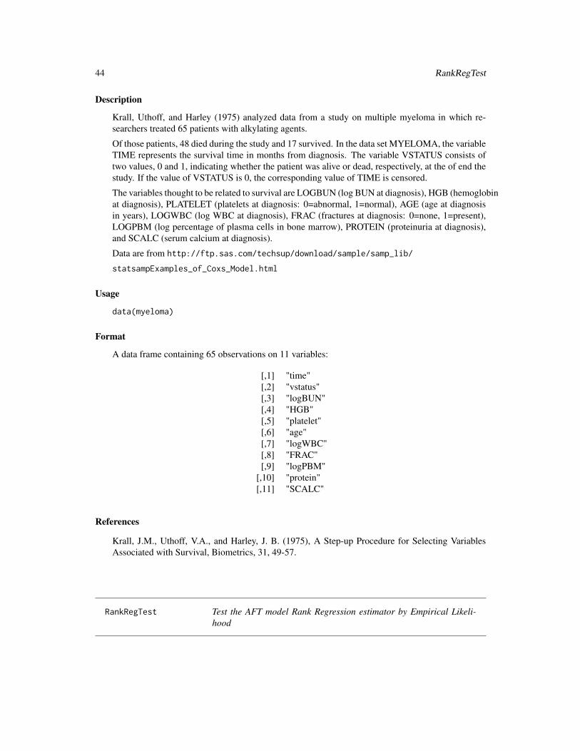
Description
Krall, Uthoff, and Harley (1975) analyzed data from a study on multiple myeloma in which re-searchers treated 65 patients with alkylating agents.
Of those patients, 48 died during the study and 17 survived. In the data set MYELOMA, the variableTIME represents the survival time in months from diagnosis. The variable VSTATUS consists oftwo values, 0 and 1, indicating whether the patient was alive or dead, respectively, at the of end thestudy. If the value of VSTATUS is 0, the corresponding value of TIME is censored.
The variables thought to be related to survival are LOGBUN (log BUN at diagnosis), HGB (hemoglobinat diagnosis), PLATELET (platelets at diagnosis: 0=abnormal, 1=normal), AGE (age at diagnosisin years), LOGWBC (log WBC at diagnosis), FRAC (fractures at diagnosis: 0=none, 1=present),LOGPBM (log percentage of plasma cells in bone marrow), PROTEIN (proteinuria at diagnosis),and SCALC (serum calcium at diagnosis).
Data are from http://ftp.sas.com/techsup/download/sample/samp_lib/
statsampExamples_of_Coxs_Model.html
Usage
data(myeloma)
Format
A data frame containing 65 observations on 11 variables:
[,1] "time"[,2] "vstatus"[,3] "logBUN"[,4] "HGB"[,5] "platelet"[,6] "age"[,7] "logWBC"[,8] "FRAC"[,9] "logPBM"
[,10] "protein"[,11] "SCALC"
References
Krall, J.M., Uthoff, V.A., and Harley, J. B. (1975), A Step-up Procedure for Selecting VariablesAssociated with Survival, Biometrics, 31, 49-57.
RankRegTest Test the AFT model Rank Regression estimator by Empirical Likeli-hood

RankRegTest 45
Description
Use the empirical likelihood ratio and Wilks theorem to test if the regression coefficient is equal tobeta, based on the rank estimator for the AFT model.
The log empirical likelihood been maximized is∑d=1
log ∆F (ei) +∑d=0
log[1 − F (ei)];
where ei are the residuals.
Usage
RankRegTest(y, d, x, beta, type="Gehan")
Arguments
y a vector of length N, containing the censored responses.
d a vector (length N) of either 1’s or 0’s. d=1 means y is uncensored; d=0 meansy is right censored.
x a matrix of size N by q.
beta a vector of length q. the value of the regression coefficient to be tested in themodel yi = βxi + εi .
type default to Gehan type. The other option is Logrank type.
Details
The estimator of beta can be obtained by function rankaft( ) in the package rankreg. But hereyou may test other values of beta. If you test the beta value that is obtained from the rankaft( ),then the -2LLR should be 0 and the p-value should be 1.
The above likelihood should be understood as the likelihood of the error term, so in the regressionmodel the error ei should be iid.
The estimation equation used when maximize the empirical likelihood is
0 =∑i
φ(ei)di∆F (ei)(xi − x̄i)/(nwi)
which was described in detail in the references below.
See also the function RankRegTestH, which is based on the hazard likelihood.
Value
A list with the following components:
"-2LLR" the -2 loglikelihood ratio; should have approximate chisq distribution under Ho.
logel2 the log empirical likelihood, under estimating equation.
logel the log empirical likelihood of the Kaplan-Meier of e’s.
prob the probabilities that max the empirical likelihood under rank estimating equa-tion constraint.
46 RankRegTestH
Author(s)
Mai Zhou.
References
Kalbfleisch, J. and Prentice, R. (2002) The Statistical Analysis of Failure Time Data. 2nd Ed. Wiley,New York. (Chapter 7)
Jin, Z., Lin, D.Y., Wei, L. J. and Ying, Z. (2003). Rank-based inference for the accelerated failuretime model. Biometrika, 90, 341-53.
Zhou, M. (2005). Empirical likelihood analysis of the rank estimator for the censored acceleratedfailure time model. Biometrika, 92, 492-98.
Examples
data(myeloma)RankRegTest(y=myeloma[,1], d=myeloma[,2], x=myeloma[,3], beta= -15.50147)# you should get "-2LLR" = 9.050426e-05 (practically zero)# The beta value, -15.50147, was obtained by rankaft() from the rankreg package.
RankRegTestH Test the AFT model, Rank Regression estimator by (Hazard)EmpiricalLikelihood
Description
Use the empirical likelihood ratio and Wilks theorem to test if the regression coefficient is equal tobeta, based on the rank estimator/estimating equation of the AFT model.
The log empirical likelihood been maximized is the hazard empirical likelihood.
Usage
RankRegTestH(y, d, x, beta, type="Gehan")
Arguments
y a vector of length N, containing the censored responses.
d a vector (length N) of either 1’s or 0’s. d=1 means y is uncensored; d=0 meansy is right censored.
x a matrix of size N by q.
beta a vector of length q. the value of the regression coefficient to be tested in themodel yi = βxi + εi .
type default to Gehan type. The other option is Logrank type.

RankRegTestH 47
Details
The estimator of beta can be obtained by function rankaft( ) in the package rankreg. But hereyou may test other values of beta. If you test the beta value that is obtained from the rankaft( ),then the -2LLR should be 0 and the p-value should be 1.
The above likelihood should be understood as the likelihood of the error term, so in the regressionmodel the error ei should be iid.
The estimating equation used when maximize the empirical likelihood is
0 =∑i
R(ei)φ(ei)di∆A(ei)(xi − x̄i)
where all notation was described in detail in the references below.
Value
A list with the following components:
"-2LLR" the -2 loglikelihood ratio; should have approximate chisq distribution under H0.
logel2 the log empirical likelihood, under estimating equation.
logel the log empirical likelihood of the Kaplan-Meier of e’s.
Author(s)
Mai Zhou
References
Zhou, M. (2016) Empirical Likelihood Methods in Survival Analysis. CRC Press.
Kalbfleisch, J. and Prentice, R. (2002) The Statistical Analysis of Failure Time Data. 2nd Ed. Wiley,New York. (Chapter 7)
Jin, Z., Lin, D.Y., Wei, L. J. and Ying, Z. (2003). Rank-based inference for the accelerated failuretime model. Biometrika, 90, 341-53.
Zhou, M. (2005). Empirical likelihood analysis of the rank estimator for the censored acceleratedfailure time model. Biometrika, 92, 492–498.
Examples
data(myeloma)RankRegTestH(y=myeloma[,1], d=myeloma[,2], x=myeloma[,3], beta= -15.50147)# you should get "-2LLR" = 9.050426e-05 (practically zero)# The beta value, -15.50147, was obtained by rankaft() from# the rankreg package.

48 ROCnp
ROCnp Test the ROC curve by Empirical Likelihood
Description
Use empirical likelihood ratio to test the hypothesis Ho: (1-b0)th quantile of sample 1 = (1-t0)thquantile of sample 2. This is the same as testing Ho: R(t0)= b0, where R(.) is the ROC curve.
The log empirical likelihood been maximized is∑d1=1
log ∆F1(t1i) +∑d1=0
log[1 − F1(t1i)] +∑d2=1
log ∆F2(t2j) +∑d2=0
log[1 − F2(t2j)].
This empirical likelihood ratio has a chi square limit under Ho.
Usage
ROCnp(t1, d1, t2, d2, b0, t0)
Arguments
t1 a vector of length n. Observed times, may be right censored.
d1 a vector of length n, censoring status. d=1 means t is uncensored; d=0 means tis right censored.
t2 a vector of length m. Observed times, may be right censored.
d2 a vector of length m, censoring status.
b0 a scalar between 0 and 1.
t0 a scalar, betwenn 0 and 1.
Details
Basically, we first test (1-b0)th quantile of sample 1 = c and also test (1-t0)th quantile of sample 2= c. This way we obtain two log likelihood ratios.
Then we minimize the sum of the two log likelihood ratio over c.
See the tech report below for details on a similar setting.
Value
A list with the following components:
"-2LLR" the -2 loglikelihood ratio; have approximate chisq distribution under Ho.
cstar the estimated common quantile.
Author(s)
Mai Zhou.

ROCnp2 49
References
Zhou, M. and Liang, H (2008). Empirical Likelihood for Hybrid Two Sample Problem with Cen-sored Data. Univ. Kentucky Tech. Report.
Su, H., Zhou, M. and Liang, H. (2011). Semi-parametric hybrid empirical likelihood inference fortwo-sample comparison with censored data. Lifetime Data Analysis, 17, 533-551.
Examples
#### An example of testing the equality of two medians. No censoring.ROCnp(t1=rexp(100), d1=rep(1,100), t2=rexp(120), d2=rep(1,120), b0=0.5, t0=0.5)############################################################################## Next, an example of finding 90 percent confidence interval of R(0.5)#### Note: We are finding confidence interval for R(0.5). So we are testing#### R(0.5)= 0.35, 0.36, 0.37, 0.38, etc. try to find values so that#### testing R(0.5) = L , U has p-value of 0.10, then [L, U] is the 90 percent#### confidence interval for R(0.5).#set.seed(123)#t1 <- rexp(200)#t2 <- rexp(200)#ROCnp( t1=t1, d1=rep(1, 200), t2=t2, d2=rep(1, 200), b0=0.5, t0=0.5)$"-2LLR"#### since the -2LLR value is less than 2.705543 = qchisq(0.9, df=1), so the#### confidence interval contains 0.5.#gridpoints <- 35:65/100#ELvalues <- gridpoints#for( i in 1:31 ) ELvalues[i] <- ROCnp(t1=t1, d1=rep(1, 200),# t2=t2, d2=rep(1, 200), b0=gridpoints[i], t0=0.5)$"-2LLR"#myfun1 <- approxfun(x=gridpoints, y=ELvalues)#uniroot( f= function(x){myfun1(x)-2.705543}, interval= c(0.35, 0.5) )#uniroot( f= function(x){myfun1(x)-2.705543}, interval= c(0.5, 0.65) )#### So, taking the two roots, we see the 90 percent confidence interval for R(0.5)#### in this case is [0.4478081, 0.5889425].
ROCnp2 Test the ROC curve by Empirical Likelihood
Description
Use empirical likelihood ratio to test the hypothesis Ho: (1-b0)th quantile of sample 1 = (1-t0)thquantile of sample 2. This is the same as testing Ho: R(t0)= b0, where R(.) is the ROC curve.
The log empirical likelihood been maximized is∑d1=1
log ∆F1(t1i) +∑d1=0
log[1 − F1(t1i)] +∑d2=1
log ∆F2(t2j) +∑d2=0
log[1 − F2(t2j)].
This empirical likelihood ratio has a chi square limit under Ho.
Usage
ROCnp2(t1, d1, t2, d2, b0, t0)

50 ROCnp2
Arguments
t1 a vector of length n. Observed times, sample 1. may be right censored.
d1 a vector of length n, censoring status. d=1 means t is uncensored; d=0 means tis right censored.
t2 a vector of length m. Observed times, sample 2. may be right censored.
d2 a vector of length m, censoring status.
b0 a scalar, between 0 and 1.
t0 a scalar, betwenn 0 and 1.
Details
First, we test (1-b0)th quantile of sample 1 = c and also test (1-t0)th quantile of sample 2 = c. Thisway we obtain two log likelihood ratios.
Then we minimize the sum of the two log likelihood ratios over c.
This version use an exhaust search for the minimum (over c). Since the objective (log lik) arepiecewise constants, the optimum( ) function in R do not work well. See the tech report below fordetails on a similar setting.
Value
A list with the following components:
"-2LLR" the -2 loglikelihood ratio; have approximate chisq distribution under Ho.
cstar the estimated common quantile.
Author(s)
Mai Zhou
References
Su, Haiyan; Zhou, Mai and Liang, Hua (2011). Semi-parametric Hybrid Empirical LikelihoodInference for Two Sample Comparison with Censored Data. Lifetime Data Analysis, 17, 533-551.
Examples
#### An example of testing the equality of two medians.#### No censoring.# ROCnp2(t1=rexp(100), d1=rep(1,100), t2=rexp(120),# d2=rep(1,120), b0=0.5, t0=0.5)################################################################### This example do not work on the Solaris Sparc machine.#### But works fine on other platforms.############### Next, an example of finding 90 percent confidence#### interval of R(0.5)#### Note: We are finding confidence interval for R(0.5).#### So we are testing

smallcell 51
#### R(0.5)= 0.35, 0.36, 0.37, 0.38, etc. try to find#### values so that testing R(0.5) = L , U has p-value#### of 0.10, then [L, U] is the 90 percent#### confidence interval for R(0.5).#set.seed(123)#t1 <- rexp(200)#t2 <- rexp(200)#ROCnp( t1=t1, d1=rep(1, 200), t2=t2, d2=rep(1, 200),# b0=0.5, t0=0.5)$"-2LLR"#### since the -2LLR value is less than#### 2.705543 = qchisq(0.9, df=1), so the#### confidence interval contains 0.5.#gridpoints <- 35:65/100#ELvalues <- gridpoints#for(i in 1:31) ELvalues[i] <- ROCnp2(t1=t1, d1=rep(1, 200),# t2=t2, d2=rep(1, 200), b0=gridpoints[i], t0=0.5)$"-2LLR"#myfun1 <- approxfun(x=gridpoints, y=ELvalues)#uniroot(f=function(x){myfun1(x)-2.705543},# interval= c(0.35, 0.5) )#uniroot(f= function(x){myfun1(x)-2.705543},# interval= c(0.5, 0.65) )#### So, taking the two roots, we see the 90 percent#### confidence interval for R(0.5) in this#### case is [0.4457862, 0.5907723].###############################################
smallcell Smallcell Lung Cancer Data
Description
There are 121 observations on 4 variables. Arm is the indication of two treatments. Entry is the ageof the patient at entry. Survival is the survival time and indicator is the censoring indicator (rightcensoring). For more details please see the reference below.
Data are from Ying, Z., Jung, SH, and Wei, LJ (1995). Median regression analysis with censoreddata. Journal of the American Statistical Association, 90, 178-184.
Usage
data(smallcell)
Format
A data frame containing 121 observations on 4 variables:
[,1] "arm"[,2] "entry"[,3] "survival"[,4] "indicator"

52 WRegEst
References
Ying, Z., Jung, SH, and Wei, LJ (1995). Median regression analysis with censored data. Journal ofthe American Statistical Association, 90, 178-184.
WRegEst Compute the casewise weighted regression estimator for AFT model
Description
For the AFT model, this function computes the case weighted estimator of beta. Either the leastsquares estimator or the regression quantile estimator.
Usage
WRegEst(x, y, delta, LS=TRUE, tau=0.5)
Arguments
x a matrix of size N by q.
y a vector of length N, containing the censored responses. Usually the log of theoriginal observed failure times.
delta a vector (length N) of either 1’s or 0’s. d=1 means y is uncensored; d=0 meansy is right censored.
LS a logical value. If TRUE then the function will return the least squares estimator.If FALSE then the function will return the quantile regression estimator, with thequantile level specified by tau. .
tau a scalar, between 0 and 1. The quantile to be used in quantile regression. Iftau=0.5 then it is the median regression. If LS=TRUE, then it is ignored.
Details
Due to the readily available minimizer, we only provide least squares and quantile regression here.However, in the companion testing function WRegTest the user can supply a self defined psifunction, corresponding to the general M-estimation in the regression modeling. (since there is nominimization needed).
The estimator is the minimizer ofn∑i=1
wiρ(Yi −Xib)
Assuming a correlation modelYi = Xiβ + σ(Xi)εi
, where ρ() is either the square or the absolute value function.
Value
The estimator β̂.
WRegTest 53
Author(s)
Mai Zhou.
References
Zhou, M.; Bathke, A. and Kim, M. (2012). Empirical likelihood analysis of the HeteroscasticAccelerated Failure Time model. Statistica Sinica, 22, 295-316.
Examples
data(smallcell)WRegEst(x=cbind(1,smallcell[,1],smallcell[,2]),
y=smallcell[,3], delta=smallcell[,4])######################################################## you should get x1 x2 x3#### -59.22126 -488.41306 16.03259####################################################WRegEst(x=cbind(1,smallcell[,1],smallcell[,2]),
y=log10(smallcell[,3]), delta=smallcell[,4], LS=FALSE)############################################################ you should get#### [1] 2.603342985 -0.263000044 0.003836832########################################################
WRegTest Test the case weighted regression estimator by Empirical Likelihood
Description
Use the empirical likelihood ratio and Wilks theorem to test if the regression coefficient is equal tobeta0, by the case weighted estimation method.
The log empirical likelihood been maximized is∑d=1
log ∆F (yi) +∑d=0
log[1 − F (yi)].
Usage
WRegTest(x, y, delta, beta0, psifun=function(t){t})
Arguments
x a matrix of size N by q. Random design matrix.
y a vector of length N, containing the censored responses.
delta a vector (length N) of either 1’s or 0’s. delta=1 means y is uncensored; delta=0means y is right censored.
beta0 a vector of length q. The value of the regression coefficient to be tested in thelinear model .

54 WRegTest
psifun the estimating function. The definition of it determines the type of estimatorunder testing.
Details
The above likelihood should be understood as the likelihood of the censored responses y and delta.
This version can handle the model where beta is a vector (of length q).
The estimation equations used when maximize the empirical likelihood is
0 =∑
δi∆F (Yi)Xi(Yi −Xiβ0)
which was described in detail in the reference below.
For median regression (Least Absolute Deviation) estimator, you should define the psifun as+1,−1 or 0 when t is > 0, < 0 or = 0.
For ordinary least squares estimator, psifun should be the identity function psifun <- function(t)t.
Value
A list with the following components:
"-2LLR" the -2 log likelihood ratio; have approximate chisq distribution under H0.
P-val the p-value using the chi-square approximation.
Author(s)
Mai Zhou.
References
Zhou, M.; Bathke, A. and Kim, M. (2012). Empirical likelihood analysis of the case weightedestimator in heteroscastic AFT model. Statistica Sinica, 22, 295-316.
Examples
xx <- c(28,-44,29,30,26,27,22,23,33,16,24,29,24,40,21,31,34,-2,25,19)

Index
∗Topic datasetsmyeloma, 43smallcell, 51
∗Topic htestBJnoint, 2bjtest, 3bjtest1d, 5bjtestII, 6el.cen.EM, 8el.cen.EM2, 10el.cen.test, 14el.ltrc.EM, 16el.test, 18el.test.wt, 20el.test.wt2, 21el.trun.test, 23emplikH.disc, 25emplikH.disc2, 27emplikH1.test, 29emplikH2.test, 31emplikHs.disc2, 33emplikHs.test2, 35findUL, 38findUL2, 40findULold, 42RankRegTest, 44RankRegTestH, 46ROCnp, 48ROCnp2, 49WRegTest, 53
∗Topic nonparametricBJnoint, 2bjtest, 3bjtest1d, 5bjtestII, 6el.cen.EM, 8el.cen.EM2, 10el.cen.test, 14el.ltrc.EM, 16
el.test, 18el.test.wt, 20el.test.wt2, 21el.trun.test, 23emplikH.disc, 25emplikH.disc2, 27emplikH1.test, 29emplikH2.test, 31emplikHs.disc2, 33emplikHs.test2, 35findUL, 38findUL2, 40findULold, 42RankRegTest, 44RankRegTestH, 46ROCnp, 48ROCnp2, 49WRegEst, 52WRegTest, 53
∗Topic survivalel.cen.EM, 8el.cen.EM2, 10el.cen.test, 14el.ltrc.EM, 16el.trun.test, 23emplikH.disc, 25emplikH.disc2, 27emplikH1.test, 29emplikH2.test, 31emplikHs.disc2, 33emplikHs.test2, 35
BJnoint, 2bjtest, 3bjtest1d, 5bjtestII, 6
el.cen.EM, 8el.cen.EM2, 10el.cen.test, 14
55

56 INDEX
el.ltrc.EM, 16el.test, 18el.test.wt, 20el.test.wt2, 21el.trun.test, 23emplikH.disc, 25emplikH.disc2, 27emplikH1.test, 29emplikH2.test, 31emplikHs.disc2, 33emplikHs.test2, 35
findUL, 38findUL2, 40findULold, 42
myeloma, 43
RankRegTest, 44RankRegTestH, 46ROCnp, 48ROCnp2, 49
smallcell, 51
WRegEst, 52WRegTest, 53
Top Related