


Languages
Pages
Legal


Option pricing andreplication withtransaction costs anddividends
Stylianos PERRAKISUniversity of Ottawa
Jean LEFOLLUniversity of Geneva
INTERNATIONAL CENTER FOR FINANCIALASSET MANAGEMENT AND ENGINEERING
Research Paper N° 8

Option pricing and replication with transaction costs and dividends
Stylianos Perrakisa and Jean Lefoll*b
a Faculty of Administration and department of economics, University of Ottawa,Ottawa, CANADA, KIN6N5
b HEC and International Finance Laboratory, University of Geneva,1211 Genève 4, SWITZERLAND
Abstract
This paper derives optimal perfect hedging portfolios in the presence of transaction costs within thebinomial model of stock returns, for a market maker that establishes bid and ask prices for Americancall options on stocks paying dividends prior to expiration. It is shown that, while the option holder'soptimal exercise policy at the ex-dividend date varies according to the stock price, there are intervals ofvalues for such a price where the optimal policy would depend on the holder's preferences.Nonetheless, the perfect hedging assumption still allows the derivation of optimal hedging portfolios forboth long and short positions of a market maker on the option.
Keywords: Pricing; Transaction costs; American options; DividendsJEL classification: G13
This version July 1999
Forthcoming in the Journal of Economic Dynamics and Control
* Corresponding author: [email protected].
Parts of the work were done while Lefoll was in sabbatical leave at the University of Ottawa during1994-95 and while Perrakis was a Visiting Professor at ALBA, Greece, during 1997-98. The authorswish to thank the Canadian Social Sciences and Humanities Research Council and the Swiss FondsNational de la Recherche Scientifique for financial support under grant #1214-040687.94, and ThierryVessereau for research assistance. A preliminary version was presented at the AFFI meetings, Tunis,June 1994, and at the NFA meetings, September 1994. We wish to thank participants at doctoralseminars at Concordia University and Université de Montréal, for helpful advice and comments. Wealso acknowledge the helpful comments from three referees and from Michaël Selby guest editor of thisissue.

EXECUTIVE SUMMARY
In a market where market makers must quote bid and ask prices, like the SOFFEX, it isimportant to be able to determine the bid and ask prices of the traded assets. This is also truefor negociated option contracts when the bid and ask prices must take transaction costs intoaccount. The methodology developed in this paper allows us to derive bid and ask prices forAmerican options on dividend-paying stocks under the assumption that the market makershedge themselves perfectly against all possible investor decisions. Since the derived prices areindependent from the market makers' preferences, including their taste for risk, the perfecthedging assumption increases the theoretical bid/ask spread. In fact, all possible spreads thatmay depend on market makers' risk aversion must lie within the perfectly hedged bid/askspread.
In an empirical study using daily data on the SOFFEX we found that the averageobserved bid/ask spreads were smaller than the theoretical spreads derived by the algorithmspresented in this article when there are dividends prior to option expiration, contrary tooptions on stocks without such dividends. From this it may be inferred that during the periodunder study the market makers did not necessarily try to hedge themselves perfectly.Nonetheless, the data show that the observed spreads were on average biased downwards andthe quoted bid prices were lower than those corresponding to perfect hedging. Given that thetheoretical prices assume that the underlying asset's price follows the binomial model, thebid/ask spread tends to increase with the number of times the market makers' portfolios arerestructured. This increases the theoretical spread because of the transaction costs incurred ineach restructuring. In order to counterbalance this effect, which is unavoidable in the binomialmodel under perfect hedging, we have adopted an ad hoc procedure of adjustment of thetransaction costs. This assumes that these costs increase at a rate that decreases in proportionto the number of times the portfolios are restructured, as specified in this article. With thisadjustment the average theoretical bid/ask spreads become comparable to those observed onthe SOFFEX. Thus, with this ad hoc adjustment of the transaction costs and with the perfecthedging hypothesis it is possible to derive bid/ask spreads comparable to those observed onthe SOFFEX, thus yielding bounds within which the market makers' spreads should liewhether or not they use perfect hedging.
The proposed algorithms allow a quick estimation of the theoretical bid and ask pricesand may thus be used by market makers on the SOFFEX. They are, to our knowledge, theonly ones that produce such prices under the perfect hedging hypothesis. The auhors have alsoextended their procedure to American put options and to options on stock indices.

1
Option Pricing and Replication with Transaction Costs and Dividends
I. Introduction
This paper derives American call option prices and replicating portfolios under transaction
costs when there are known dividends prior to option expiration. It thus extends similar derivations
for European options originally introduced by Merton (1989), and subsequently extended by Boyle
and Vorst (1992, BV), Bensaid et al (1992, BLPS), and Perrakis and Lefoll (1997a, PL).
The notion of option replication underlies the two main option pricing models in financial
theory, the continuous-time Black and Scholes (1973) model, and the binomial model of Cox, Ross
and Rubinstein (1979) and Rendleman and Bartter (1979). The European call option price is
derived by constructing a portfolio that includes the stock and the riskless asset, whose return
characteristics replicate exactly those of the option, under the assumption that there are no
transaction costs. This assumption cannot be relaxed easily. Transactions costs manifest themselves
on the side of the underlying stock by the existence not of a single price, but of an interval of prices
contained within the bid and ask price of the stock. An option pricing model that incorporates
transactions costs should derive the option bid and ask prices from the bid and ask prices of the
underlying stock, as well as from other possible transactions costs.
This kind of derivation was first attempted by Merton (1989) for a binomial model that had
only two periods till option expiration, by assuming that options are produced by financial
intermediaries under perfect hedging. These intermediaries replicate the option with a stock-plus-
riskless asset portfolio that incorporates proportional transactions costs when changing the stock
holdings; in this way they hedge their positions perfectly, namely they make sure that they have

2
sufficient cash to cover their obligations under all circumstances. Two such portfolios are issued, for
the option buyers and the option writers respectively, corresponding ultimately to the ask and bid
prices of the option.
The Merton derivations were extended to any number of periods to expiration in the BV
and BLPS studies. While the BV study used exact replication, BLPS pointed out that it may not be
optimal to replicate the option to obtain perfect hedging: by not rebalancing the portfolio the
intermediary avoids some transactions costs, ending up with more cash at expiration than required
by perfect hedging. BLPS developed algorithms for optimal portfolio rebalancing in the presence
of transactions costs when the option is at least perfectly hedged; such strategies are known as
super-replication. They also derived conditions for the optimality of exact option replication. The
PL study extended their approach to cases of non-convexity of the final constraints.
In this paper option prices and super-replicating portfolios1 are derived in a binomial model
with transactions costs when there are known dividends to be paid to the stockholders at given
times prior to the expiration of the option. The derived portfolios super-replicate investors' long and
short positions in options under such conditions. It is well known since Merton (1973) that in such
cases the European and American call options do not have the same price, and that the American
option may be either prematurely exercised at the ex-dividend date, or left unexercised till
expiration. Option prices with dividends in the absence of transactions costs were derived by Roll
(1977), Geske (1979), and Whaley (1981), and extended by Selby and Hodges (1987), in the
context of the Black-Scholes model. This paper bears the same relationship to the Merton, BV and
BLPS studies as Roll, Geske, and Whaley to the Black-Scholes model. As with the earlier studies,
its main contribution is the identification of the early exercise boundary, the stock prices at ex-
dividend dates that separate early from deferred exercise. The introduction of transaction costs

3
makes this boundary rather complex, insofar as there is now a region of such stock prices, rather
than a single price, at each ex-dividend date: there is immediate (deferred) exercise above (below)
this region, while within it the exercise depends on whether the last move was an up or a down.
Before closing this brief survey of the literature, we note some alternative approaches to
option pricing with transactions costs. An early study by Leland (1985) derived an approximate
option replication model under transaction costs within the continuous-time Black-Scholes model.
Leland assumed an exogenously-given finite number of portfolio rebalancing periods, which did
not constitute a perfectly-hedged position, with sufficient cash to cover all terminal option values.
More recently Soner et al (1995) showed that the value of the portfolio replicating the long option
in continuous time tends to the stock price for any finite transaction cost.
Other studies are based on optimizing portfolio choice (including options) for a given
investor utility function. In contrast to perfect hedging, the resulting option reservation price would
depend on the investor wealth and utility function used in the derivations. Examples of such an
approach are Hodges and Neuberger (1989), Dumas and Luciano (1991), and Constantinides
(1986). This approach has not been able till now to derive equilibrium option bid and ask prices. As
Davis et al. (1993) point out, there are theoretical issues that remain unsolved, since the reservation
prices for option buyers and writers define an empty set of equilibrium prices.
On the other hand, the main weakness of the perfectly-hedged binomial-based approaches
to option pricing under transaction costs is the need to specify exogenously the number of steps in
the binomial tree. This is a potentially fatal flaw, since the bid/ask spread increases with this
number of steps. At the limit the ask price tends to the stock price, while the bid price is equal to
the well-known Merton (1973) lower bound for finite values of binomial time steps2.

4
A possible solution was proposed by Henrotte (1993) and Flesaker and Hughston (1994),
who proposed replacing the fixed transaction cost parameter by one that declines in proportion to
the square root of the number of binomial steps. This method is the only one so far that produces
reasonable non-trivial option prices under transaction costs, both in continuous time and on
binomial lattices. It serves as the main justification for the approach adopted in this paper, although
the algorithms developed here do not depend on it. Further, several technical conditions necessary
for our results are satisfied for reasonable parameter values under such an assumption.
In the next section we present the general model and review the results available for option
pricing and replication in the binomial model in the presence of transactions costs and without any
dividends. A single dividend is introduced in sections III and IV, for the long and short calls
respectively, while section V extends the results to any number of dividends and presents some
numerical examples. The proofs of the main results are given in summary form in the appendix.
More detailed proofs of these results are available from our working paper (Perrakis and Lefoll,
1997b).
II. The General Model
Let u, d and R denote the three parameters of the binomial process, denoting respectively
the size of the up and down moves, and one plus the riskless rate of interest, with d<R<u. Let also k
denote the transactions cost parameter, assumed for simplicity the same for sales and purchases of
stock. This implies that the purchase of $1 of shares costs $(1+k), while the short sale of $1 of
shares yields $(1-k); we assume that there are no transactions costs in the riskless asset. The
exercise price of the option is X, and T is the expiration time of the option (in number of periods).
At some time τ∈(0,T) there is a dividend D that is paid3; this dividend can be constant in dollar or

5
in yield terms, or any other function of the stock price at the ex-dividend date. Hence, if Sτ is the
price of the stock at τ the subsequent values of the stock price follow the initial binomial process,
with starting price4 Sτ-D, assumed positive for all possible Sτ. Let also S0 denote the initial stock
price. Our purpose is to derive the values of portfolios that super-replicate investors’ long and short
positions in the American option on such a stock; denoted by the subscripts a and b respectively. If
the options are issued by a perfectly-hedged financial intermediary, as in Merton (1989), then their
respective ask and bid prices are Cad(S0,T) and Cbd(S0,T), with the subscript d denoting the presence
of a dividend.
Similarly, we denote by Ca(S0,n) and Cb(S0,n) the corresponding ask and bid prices when
the initial stock price is S0, the expiration time is n, and there are no dividends prior to expiration of
the option. In other words, if Nj and Bj denote respectively the number of shares and amount of
cash at time j∈[0,n] in the super-replicating portfolios of long and short options, we have
Ca(S0,n)=N0aS0+B0a, Cb(S0,n) = -(N0bS0+B0b), and the terminal portfolios (Nn,Bn) are respectively
equal to (1,-X) and (-1,X) for Ca and Cb, or to (0,0) in both cases, depending on the terminal value
of Sn . The values Ca and Cb are in this case equal to those of the corresponding European options,
and were derived in the previously-mentioned studies of Merton (1989), BV and BLPS.
In the BV study these derivations were by replication at every node of the binomial tree.
However, their derivation for the short call is valid if and only if the following conditions hold5:
d(1+k)≤R(1-k),(1)
R(1+k)≤u(1-k).
In the more general formulation of the BLPS study it was shown that replication is an
optimal perfect hedging policy only for long call options with physical delivery of the asset, and for

6
all European options when (1) holds. Otherwise, for short calls with physical delivery, and for both
long and short calls with cash settlement, super-replication implies that it may be optimal not to
rebalance the stock-plus-riskless asset portfolio at every node in order to save on transactions costs.
A key assumption of the BLPS study is that the optimal policy at option expiration be
prespecified as a function of the terminal stock price Sn. This assumption was relaxed in PL, where
it was shown that it is inconsistent with the perfect hedging requirement when there are transactions
costs. For instance, for Sn∈[X/(1+k),X/(1-k)] an option holder may or may not exercise the option,
depending on his/her preference for holding stock or cash6 at time n; perfect hedging implies that
the intermediary must have enough cash to hedge either one of these two positions. In American
options this dependence appears at every node of the binomial tree, thus requiring a major
reformulation of the BLPS approach.
Relations (1) are important technical conditions on the binomial parameters, affecting the
optimal hedging policies. In the PL study it was shown that BLPS algorithm may no longer be
valid when (1) is violated, due to the presence of non-convexities in the final constraints in the
program (4)-(5) below. When these constraints are non-convex the BLPS algorithm can identify
only local minima of the objective function at every node of the binomial tree. For such cases PL
derived an extension of the BLPS algorithm, that showed that the option bid price coincided with
the well-known Merton lower bound for European calls, Max{0,S0-X/Rn}, when the following
inequality holds:
(2) d(1+k)>u(1-k).

7
In this paper it will be assumed that (1) holds, even though this is not necessary for all the derived
results. The violations of (1) are discussed as an extension, and it is shown that when (2) holds the
derived option bid and ask prices assume trivial values.
Let ωj denote a particular path from 0 to j∈[1,n], i.e. a particular sequence of up and down
moves, and Sj(ωj) the corresponding stock price; clearly, ωj+1=uωj or dωj. Following BLPS, we
model the transactions costs by means of the function φ(y), which is equal to (1+k)y for y≥0 and to
(1-k)y for y≤0. Then for any time j the hedging portfolio must contain enough cash in the riskless
asset to cover the subsequent position, including the transactions cost. This implies that:
(3) RBj≥Bj+1+φ(Nj+1-Nj)Sj+1(ωj+1),
where (Nj,Bj) are dependent on the path ωj. At expiration, for the long call with physical delivery
the terminal portfolio (Nn,Bn) is equal to (1,-X) when (1-k)Sn≥X and to (0,0) when (1+k)Sn≤X,
since all option holders will unequivocally exercise or let expire the option. For intermediate values
of Sn, however, the option holders may or may not exercise the option, and the cash must be
sufficient to hedge either action; this implies that RBn-1≥Max{-X+φ(1-Nn-1)Sn(ωn),φ(-Nn-1)Sn(ωn)}
for Sn∈(X/(1+k),X/(1-k)). The BLPS algorithm computes sequentially the optimal path-dependent
portfolios by evaluating for each path the following function:
(4) Qj(Nj-1,ωj)=Min{Bj+φ(Nj-Nj-1)Sj(ωj)} Nj,Bj
subject to
(5) RBj≥Max{Qj+1(Nj,uωj),Qj+1(Nj,dωj)}.
8
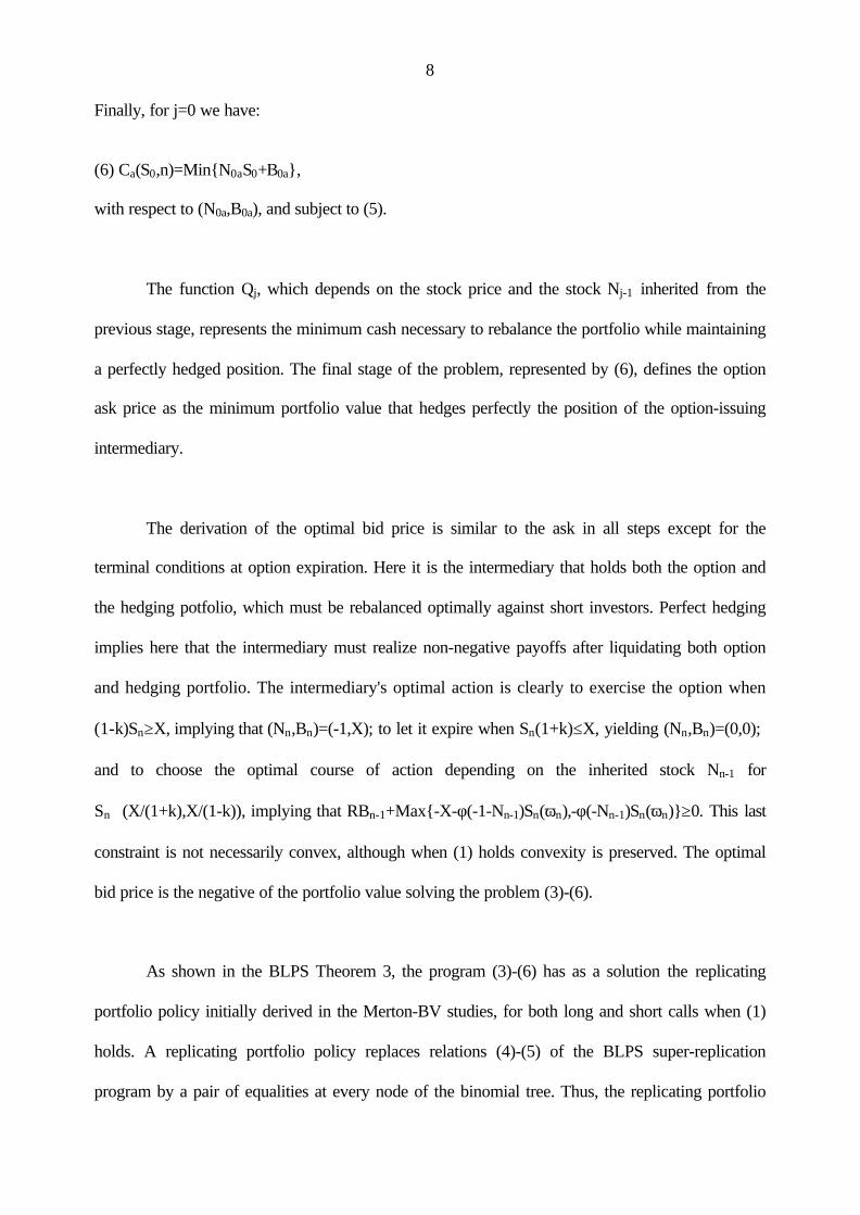
Finally, for j=0 we have:
(6) Ca(S0,n)=Min{N0aS0+B0a},
with respect to (N0a,B0a), and subject to (5).
The function Qj, which depends on the stock price and the stock Nj-1 inherited from the
previous stage, represents the minimum cash necessary to rebalance the portfolio while maintaining
a perfectly hedged position. The final stage of the problem, represented by (6), defines the option
ask price as the minimum portfolio value that hedges perfectly the position of the option-issuing
intermediary.
The derivation of the optimal bid price is similar to the ask in all steps except for the
terminal conditions at option expiration. Here it is the intermediary that holds both the option and
the hedging potfolio, which must be rebalanced optimally against short investors. Perfect hedging
implies here that the intermediary must realize non-negative payoffs after liquidating both option
and hedging portfolio. The intermediary's optimal action is clearly to exercise the option when
(1-k)Sn≥X, implying that (Nn,Bn)=(-1,X); to let it expire when Sn(1+k)≤X, yielding (Nn,Bn)=(0,0);
and to choose the optimal course of action depending on the inherited stock Nn-1 for
Sn∈(X/(1+k),X/(1-k)), implying that RBn-1+Max{-X-φ(-1-Nn-1)Sn(ωn),-φ(-Nn-1)Sn(ωn)}≥0. This last
constraint is not necessarily convex, although when (1) holds convexity is preserved. The optimal
bid price is the negative of the portfolio value solving the problem (3)-(6).
As shown in the BLPS Theorem 3, the program (3)-(6) has as a solution the replicating
portfolio policy initially derived in the Merton-BV studies, for both long and short calls when (1)
holds. A replicating portfolio policy replaces relations (4)-(5) of the BLPS super-replication
program by a pair of equalities at every node of the binomial tree. Thus, the replicating portfolio

9
(N,B) at any node S is found recursively from the portfolios (Ni,Bi) of the successor nodes Si, i=1,2,
with S1=uS, S2=dS, by means of relations (4)-(6) of BV, which are reproduced here:
NSu(1+k)+BR=N1Su(1+k)+B1 ,(7a)
NSd(1-k)+BR=N2Sd(1-k)+B2 ,
for the ask price, and
NSu(1-k)+BR=N1Su(1-k)+B1 ,(7b)
NSd(1+k)+BR=N2Sd(1+k)+B2 ,
for the bid price when (1) holds.
Before introducing the dividends we need some auxiliary results pertaining to the properties
of Ca(S0,n) and Cb(S0.n) as functions of the initial stock price S0. Indeed, if the option is not
exercised at the ex-dividend date when the stock has value Sτ, it will be hedged optimally by a
portfolio with value equal to Ca(Sτ-D,T-τ). This is a function defined on the sequence of points Sτ
generated by the binomial tree at the ex-dividend date. After that date the properties of the
unexercised option as a function of Sτ will determine the option holder's optimal policy at τ, as it
will be shown in the next section. Similar considerations apply also for the option's bid price.
The following auxiliary results are similar to well-known properties of European calls7, and
will play a role when dividends are introduced.
Lemma 1. Ca(S0,n) is increasing and convex in S0, and ∂Ca/∂S0 ≤1. Further, N0a is non-decreasing
and B0a is non-increasing in S0, with Max{N0a}=1 and Min{B0a}=-X/Rn for S0dn≥X/(1-k).
Proof. See appendix.

10
Lemma 2. When either (1) or (2) hold then Cb(S0,n) is increasing and convex in S0, ∂Cb/∂S0 ≤1,
while -N0b is non-decreasing and -B0b is non-increasing in S0, with Max{-N0b}=1 and
Min{-Bob}= X/Rn. Further, in all cases Cb(S0,n)≤Ca(S0,n).
Proof. See appendix.
Lemma 3. The functions B0a+(1+k)N0aS0≡Ca+(S0) and B0a+(1-k)NoaS0≡Ca-(S0) are non-
negative, non-decreasing and convex in S0. The same properties also hold for the functions
[-B0b-(1+k)N0bS0]≡Cb+(S0) and [-B0b-(1-k)NobS0]≡Cb-(S0), but only when (1) is true.
Proof. See appendix.
These three lemmas establish very useful properties for the results to be derived in the next
section. In particular, any initial stock price and time to option expiration in a binomial model
define automatically a pair of portfolios, one of which replicates the long option, and the other
hedges perfectly and optimally the short option. Both portfolios can be assumed known in any
given case; they will be used in finding the option bid and ask values when a dividend exists prior
to expiration.
III. Ask Prices for American Calls with Transactions Costs and a Single Dividend
Let Sτ∈[S0dτ,S0uτ] denote the stock price at the ex-dividend date. If the option is exercised
the option holder (which can be the intermediary or an investor) receives a portfolio (1,-X).
Otherwise, the stock price model becomes binomial with initial price Sτ-D, and the option's
expiration time is T-τ. This last option has no dividends till expiration; hence, it is equivalent to an
option on a binomial stock with starting price Sτ-D, that delivers the portfolio (1,-X) in T-τ periods.
As discussed in the previous section, if this option is held by an investor then it can be hedged

11
perfectly at τ by the intermediary by a portfolio (Nτa,Bτa) that replicates exactly the call, and whose
value is Nτa(Sτ-D)+Bτa=Ca(Sτ-D,T-τ).
The intermediary, which sells the option at the ask price, must hedge its position against
either action by the investor. Conversely, the intermediary holds a long position with respect to
option writers; it is perfectly hedged if it adopts the best policy (from its point of view) in each
case. We know from the previous section that, if it does not exercise at τ, its optimal hedging
portfolio is (Nτb,Bτb), that may or may not replicate the option depending on the values of the
parameters; in either case its value is -[Nτb(Sτ-D)+Bτb]=Cb(Sτ-D,T-τ).
Consider first the intermediary's hedging policy for investors having a long position on the
option. These investors would choose to exercise the option at τ or hold it till expiration, depending
on which alternative is more profitable. Clearly, if Sτ(1-k)-X≥Ca(Sτ-D,T-τ) it is unequivocally
better to exercise. Similarly, if Sτ(1+k)-X≤Cb(Sτ-D,T-τ) the holder is better-off not exercising (he
can do better by selling the unexercised option and buying one share of the stock). In-between the
optimal decision depends on the holder's preference between holding stock at τ or at T. For the
intermediary to be perfectly hedged the cash available at time τ should be sufficient to hedge either
position. The key issue is to define the ranges of values of Sτ∈[S0dτ,S0uτ] for which these actions
are optimal.
By Lemma 1 Ca(Sτ-D,T-τ) becomes asymptotically equal to its lower bound, Sτ-D-X/RT-τ for
sufficiently large Sτ. Similarly, by lemma 2 Cb(Sτ-D,T-τ) is either exactly equal to that same
expression when (2) holds, or becomes asymptotically equal to it for sufficiently large Sτ when (1)
holds. Hence, X/(1+k)≥D+X/RT-τ is a necessary condition for Cb(Sτ-D,T-τ) to be greater than or

12
equal to Sτ(1+k)-X for all Sτ, implying that the option holder would never exercise the call at τ. For
exercise at τ to be profitable for all investors for some Sτ, on the other hand, we must have X/(1-
k)<D+X/RT-τ.
We shall assume that this last inequality holds, since all other cases are special cases of it.
Then the regions of values of Sτ that delineate the appropriate optimal option exercise policies
depend on the intersection of the convex function Ca(Sτ-D,T-τ) with the line Sτ(1-k)-X; this
intersection can have 0, 1 or 2 common points. If Sτ(1-k)-X intersects Sτ-D-X/RT-τ above the point
where the latter becomes equal to Ca(Sτ-D,T-τ), as in Figure 1, then there is only one such
intersection point, denoted by Sτ2, while Sτ1 denotes the intersection of Sτ(1+k)-X and Cb(Sτ-D,T-τ).
There may also be two intersection points8, Sτ2 and Sτ3, or no intersection point, when the entire
function Ca(Sτ-D,T-τ) lies above the line Sτ(1-k)-X. We shall use the case depicted in Figure 1 as
our base case (see note 8).The key issue is the location of the points Sτi, i=1,2, with respect to the
interval [S0dτ,S0uτ].
Suppose that we are as in Figure 1. If both points are within that interval then immediate
exercise is clearly profitable for all option holders for Sτ≥Sτ2. Similarly, all option holders would
choose not to exercise for Sτ≤Sτ1. For Sτ∈(Sτ1,Sτ2), on the other hand, some investors may choose
to exercise and others may not, and the intermediary must be hedged against either action.
Accordingly, the intermediary's position at τ should be as follows:
deliver (Nτ,Bτ)=(1,-X) for Sτ ≥ Sτ2;
hold (Nτ,Bτ)=(Nτa,Bτa) for Sτ ≤ Sτ1, where (Nτa,Bτa) represents the long option-replicating portfolio9,
corresponding to a starting stock price of (Sτ-D) and a maturity of T-τ;
have enough cash at τ to hedge either one of these two deliveries for Sτ∈(Sτ1,Sτ2) .

13
Figure 1
The two values Sτ2 and Sτ1 are, respectively, the lowest Sτ satisfying Sτ(1-k)-X≥Ca(Sτ-D,T-τ), and
the highest Sτ satisfying Sτ(1+k)-X≤Cb(Sτ-D,T-τ). The existence of the points Sτi, i=1,2, within the
interval of admissible values of Sτ will depend on the given values of S0, X, u, d, R, D, T and τ. If
any one of those points does not exist within the appropriate interval (as, for instance, when Ca(Sτ-
D,T-τ) lies entirely above Sτ(1-k)-X) then the intermediary's optimal policy would cover only some
of the above actions.
We can now derive the ask price for the call with dividends, Cad(S0,T), which can be found
after the situation prevailing at the ex-dividend date τ has been established. It is found from the
following program:
(P1) Cad(S0,T)=Min{N0S0+B0}, subject to RBj-1(ωj)-Bj(ωj)≥φ(Nj(ωj)-Nj-1(ωj))Sj(ωj) for every j≤τ-1
and for every path ωj.
At j=τ, and for the situation depicted in Figure 1, the above constraint is replaced by the following:
(8a) RBτ-1≥-X+φ(1-Nτ-1)Sτ(ωτ), Sτ(ωτ)∈{[S0dτ,S0uτ]∩[Sτ;Sτ(ωτ)>Sτ2]};
(8b) RBτ-1≥Bτa+φ(Nτa-Nτ-1)[Sτ(ωτ)-D]-DNτ-1, Sτ(ωτ)∈{[S0dτ,S0uτ]∩[Sτ;Sτ(ωτ)≤Sτ1]};
(8c) RBτ-1≥Max{-X+φ(1-Nτ-1)Sτ(ωτ), Bτa+φ(Nτa-Nτ-1)[Sτ(ωτ)-D]-DNτ-1} for Sτ(ωτ)∈{[S0dτ,S0uτ]∩(Sτ1,Sτ2)}.
We note that at τ-1 the portfolio (Nτ-1,Bτ-1) that hedges the option is entitled to the dividend even if
the option holder decides not to exercise, thus accounting for the extra cash DNτ-1 in the RHS of
(8a,b,c). Let Wm(Nτ-1, Sτ) denote the RHS of (8m), m=a,b.
14
The program (P1) is an adaptation of the BLPS algorithm for the dividend case with a
horizon at the x-dividend date τ, with a few important differences. Thus, although there is still
physical delivery of the option in some terminal states, the terminal portfolio (Nτ,Bτ) is no longer
prespecified. Nonetheless, the RHS of the constraints (8a,b,c) is convex in Nτ-1, since it is the
maximum of two convex functions. Hence, by setting Qτ(Nτ-1,ωτ)≡ RHS of (8a,b,c), we note that
Qτ is convex in Nτ-1, implying that Lemma 5 of BLPS is valid, and Qj(Nj-1,ωj) as given by (4) is
valid for all j≤τ-1.
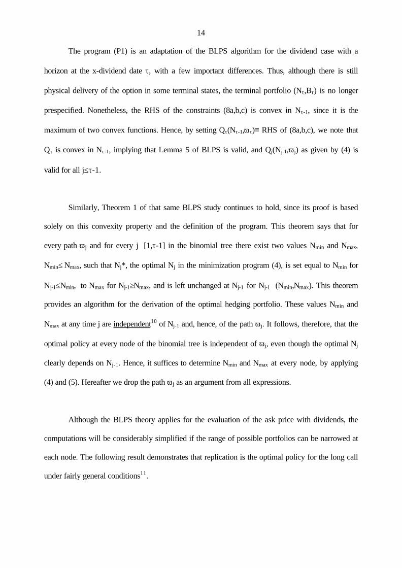
Similarly, Theorem 1 of that same BLPS study continues to hold, since its proof is based
solely on this convexity property and the definition of the program. This theorem says that for
every path ωj and for every j∈[1,τ-1] in the binomial tree there exist two values Nmin and Nmax,
Nmin≤ Nmax, such that Nj*, the optimal Nj in the minimization program (4), is set equal to Nmin for
Nj-1≤Nmin, to Nmax for Nj-1≥Nmax, and is left unchanged at Nj-1 for Nj-1∈(Nmin,Nmax). This theorem
provides an algorithm for the derivation of the optimal hedging portfolio. These values Nmin and
Nmax at any time j are independent10 of Nj-1 and, hence, of the path ωj. It follows, therefore, that the
optimal policy at every node of the binomial tree is independent of ωj, even though the optimal Nj
clearly depends on Nj-1. Hence, it suffices to determine Nmin and Nmax at every node, by applying
(4) and (5). Hereafter we drop the path ωj as an argument from all expressions.
Although the BLPS theory applies for the evaluation of the ask price with dividends, the
computations will be considerably simplified if the range of possible portfolios can be narrowed at
each node. The following result demonstrates that replication is the optimal policy for the long call
under fairly general conditions11.

15
Theorem 1. Assume that:
R(1+k)<u(1+k)-kD/Sτ-1,(9)
R(1-k)>d(1-k)+kD/Sτ-1.
Then a unique option replicating portfolio in the presence of dividends exists and is the optimal
perfectly-hedging policy for the long call if inequalities (9) hold.
Proof. See appendix.
The validity of this theorem depends on the technical conditions (9), since if these
conditions do not hold in a strict form the optimal hedging policy is not necessarily unique. A direct
comparison of (1) and (9) shows that (1) implies (9) if 2Sτ-1≥D, which obviously holds. On the
other hand, for general parameter values (9) is not necessarily a weaker inequality than (2). Under
the commonly used definition of u, d and R shown in (12) below, however, it can be shown that (9)
holds also under (2) for most reasonable values of k and the dividend rate. This is discussed further
in section V.
Thus, the replicating portfolio emerges as a solution to the optimal hedging problem for the
asking price of an option in the presence of dividends when conditions (9) hold. The main
difference with the no-dividend case in computing the option ask price Cad lies at the ex-dividend
time, at which the perfectly-hedging intermediary must be prepared to restructure its hedging
portfolio to face either delivery of the stock, or default to the optimal hedging portfolio after the
dividend has been paid. The recursive relations needed to evaluate the replicating portfolio at time
τ-1 differ from those applicable to all time periods j∈[0,τ-2], where the optimal hedging portfolio is
derived by applying relations (7a). By contrast, at τ-1 the form of the equations determining the
optimal portfolio (Nτ-1*,Bτ-1*) depends on the location of the successor nodes Sτ with respect to the
intervals defined in the RHS of (8a,b,c). For instance, for uSτ-1≤Sτ1 the optimal portfolio at τ-1 must

16
replicate portfolios that, in turn, replicate the options expiring at T with starting stock prices uSτ-1-D
and dSτ-1-D. Similarly, when both uSτ-1 and dSτ-1 lie above Sτ2, the optimal portfolio at τ-1
replicates the portfolio (1,-X). In this last case it is clear that (7a) still apply. In all other cases,
though, these relations must be modified to take into account the existence of dividends.
When at least one of the successor nodes of Sτ-1 lies within the interval (Sτ1,Sτ2) the
portfolio (Nτ-1*,Bτ-1*) replicates a position that may correspond to immediate or deferred exercises
for both successor nodes, or to immediate exercise for an up move and deferred exercise for a down
move. It can be shown that the constraints Wb(Nτ-1,uSτ-1) and Wb(Nτ-1,dSτ-1) intersect at a single
value of Nτ-1 that lies within the interval [Nτa(d),Nτa(u)]; the corresponding portfolio is given by the
system:
(10a) u(1+k)Sτ-1Nτ-1+RBτ-1-kDNτ-1=(1+k)Nτa(u)(uSτ-1-D)+Bτa(u),
(10b) d(1-k)Sτ-1Nτ-1+RBτ-1+kDNτ-1=(1-k)Nτa(d)(dSτ-1-D)+Bτa(d),
with deferred exercise in both successor nodes, as in equation (8b). The only other possibility is
when Wa(Nτ-1,uSτ-1) intersects with Wb(Nτ-1,dSτ-1) at a value Nτ-1>Nτa(d). This intersection defines a
portfolio replicating immediate and deferred exercise for up and down moves respectively, with
corresponding stockholdings Nτ =1 and Nτ =Nτa(d) ; it is given by the system:
(11a) u(1+k)Sτ-1Nτ-1+RBτ-1=u(1+k)Sτ-1-X ,
(11b) (same as (10b)).

17
It can be easily seen that when at least one of uSτ-1 or dSτ-1 lies within the interval (Sτ1,Sτ2) the
optimal replicating portfolio (Nτ-1*,Bτ-1*) is the one corresponding to the largest Nτ-1 solving
(10a,b) or (11a,b). Further, it can be shown that if (11a,b) is the appropriate system for some value
of Sτ-1 then (10a,b) cannot be the appropriate system for any higher values of Sτ-1.
Hence, the early exercise boundary, which is a single value of the stock price in the absence
of transaction costs, is now replaced by the set of values (Sτ1,Sτ2) of the stock price at time τ, which
define the regions {Sτ:Sτ≤Sτ1}, {Sτ:Sτ≥Sτ2}, {Sτ:Sτ∈(Sτ1,Sτ2)}. These can be easily translated to
corresponding intervals of values of Sτ-1. For Sτ-1∈(Sτ1/u,Sτ2/d) there exists a (possibly empty)
subinterval [Sτ-1,1,Sτ-1,2]⊂(Sτ1/u,Sτ2/d) of values of Sτ-1, such that (Nτ-1*,Bτ-1*)=(1,-X) for Sτ-1≥Sτ-1,2,
(Nτ-1*,Bτ-1*) is the solution of (10a,b) for Sτ-1≤Sτ-1,1, and (Nτ-1*,Bτ-1*) is the solution of (11a,b) for
Sτ-1∈(Sτ-1,1,Sτ-1,2). Once (Nτ-1*,Bτ-1*) have been defined at every node, we find (Nj*, Bj*) for
j∈[0,τ-2] by applying (7a).
Example. Let S0=X=100, R=1, T=3, u=1.05, d=1/u, D=5, τ=2, k=6%. The corresponding
binomial tree is shown in Figure 2, together with the three values of Ca(Sτ-D,1) at τ, at the nodes
labelled 1,2,3; the bid prices at τ for the unexercised calls are given by the Merton bound
Max{0, Sτ-D-X/R}, which is 0 at nodes 2 and 3 and equal to 5.25 at node 1. The values Cai(Sτ-
D,1), i=1,2, are found by applying the system (7a) with N1=1, B1=-X/R, N2=B2=0, to the
corresponding nodes; for instance, for S=105.25 the solution of (7a) yields N=0.748, B=-70.477.
With these values it is clear that at τ we have Ca(Sτ-D,T-τ)>Sτ(1-k)-X at nodes 1 and 2, while
Sτ1 coincides with node 3 in Figure 2. Hence, in both nodes 1 and 2 the intermediary may face
either immediate or deferred exercise, and we need to determine by applying (8c) which one of
the two will impose the heaviest cash requirements. At node 1 Wa(Nτ-1,S1)=-100+110.25

18
(1-Nτ-1)1.06>Wb(Nτ-1,S1)=-70.477-5Nτ-1+105.25φ(0.748-Nτ-1) for all Nτ-1∈[0,1], while at
point 2 Wa(0,S2)>Wb(0,S2) but Wa(1,S2)<Wb(1,S2). At node 1, therefore, the intermediary
should hedge against immediate exercise, at node 3 against deferred exercise, and at node 2
against both immediate and deferred exercise depending on Nτ-1. Hence, at τ-1 the hedging
portfolios for the two paths originating from each one of the nodes A and B are found by solving
system (11a,b) at both nodes, yielding NA*=0.6952, BA*=-64.384, NB*=0.2154, BB*=-18.426.
Last, at the origin we get by applying (7a) that N0=0.5574, B0=-46.092, yielding Cad=9.652.
Figure 2
Next we examine the limiting form of the call ask price when the number of periods to the
ex-dividend date becomes very large. Here it will be ultimately assumed12 that the dividend is a
constant proportion γ of Sτ, where γ satisfies (9). The limiting process of the binomial model is as in
Cox, Ross and Rubinstein (1979), with u, d and R given by
(12) u=eσ√h, d=1/u, R=erh,
where h≡t/τ=(t1-t)/(T-τ), t and t1 are the continuous times to ex-dividend date and option expiration
respectively, τ and T are the numbers of discrete periods within t and t1, σ is the volatility of the
stock, and r is the riskless rate of interest.
As in BV pp. 274-276, the evaluation of the replicating portfolio corresponds to a
discounted expectation under a modified Markovian process, in which the transition probabilities
depend on the previous move. The Markovian process consists of a sequence of random variables
x1,...,xτ, each one of which can have only two states with values lnu and lnd. The stock price Sτ is

19
equal to S0eY, where Y=Σxj. In the appendix it is shown that Cad may be approximated by the
following expression, with the expectation taken with respect to the random variable Y:
(13) Cad=R-τE{Max[S0eY-X,Bτa+Nτa(1-γ)S0eY]}.
For k=0 expression (13) becomes the value of an American call option with a single
proportional dividend payable at τ under the binomial model. It is well-known13 that no closed-
form solution exists for the limiting form of the value of such a call option when τ→∞. American
calls with dividends are generally evaluated by the Roll-Geske-Whaley (RGW) procedure, which
takes the discounted risk-neutral expectation of the maximum of the immediate and deferred
exercise values of the option at the ex-dividend date, under the lognormal distribution that forms
the limit14 of the binomial process (12). (13), therefore, does not converge to a closed-form
expression. It can be shown, on the other hand, that for a large τ an approximate limiting lognormal
distribution of the stock price Sτ exists under our process, similar to the limiting distribution of (12)
but incorporating the transactions costs. The limiting form of Cad is then expressed by the following
result.
Theorem 2. For large τ and T-τ and small k the ask price Cad of a call option issued by a perfectly-
hedged intermediary when there is a constant dividend yield γ policy at t can be approximated by a
modified1 5 RGW procedure, ie. by e- r t times the expectation of the function
Max{St -X,Ca((1-γ)St,t1-t)}, the latter evaluated with a risk-neutral lognormal distribution with
variance σ2[1 + (2k√τ)/(σ√t)]. This approximation has the same relationship to the discrete process
used in (13) as the original RGW approach has to the binomial American call option value.
Proof. See appendix.

20
Theorem 2 provides an easy way of extending the RGW procedure in order to approximate
the call ask price in the presence of dividends. Of particular interest are approximations
incorporating the Henrotte-Flesaker and Hughston assumption that the transaction cost parameter
varies inversely with the number of binomial periods to ex-dividend date or to option expiration. In
our notation this means that k=κ√h, where κ is a constant parameter, implying that the variance of
the limiting lognormal process is σ2(1+2κ/σ). Examples of the accuracy of the approximation for
various values of t, k and/or κ are given in Section V.
IV. Bid Prices for American Calls With a Single Dividend
The optimal perfect hedging policy is somewhat different for the short call with dividends.
Here it is the intermediary that has the choice of exercising the option at τ or holding it till
expiration. Nonetheless, the stock price limits Sτi, i=1,2,3 are still valid in terms of the optimality of
the exercise policy. At the ex-dividend time τ the intermediary finds itself holding a call option plus
the hedging portfolio. It can exercise the option or hold it till expiration, in which case it must also
restructure the portfolio, so that it guarantees non-negative payoffs at T. The optimal hedging
portfolio at τ is the one that corresponds to the best policy, of exercising or restructuring and
waiting till T.
As in the no-dividend case, we treat separately the two cases where either (1) or (2) hold. If
(1) hold then the optimal hedging portfolio at τ, if the option is not exercised, is independent of the
holdings (Nτ-1,Bτ-1), and is equal to the portfolio (Nτb,Bτb). This is the optimal hedging portfolio for
a short option without dividends, expiring T-τ periods later with exercise price X and starting stock

21
price Sτ-D. By contrast, the optimal hedging policy for such an option when (2) holds is dependent
on the holdings (Nτ-1,Bτ-1).
In all cases the bid price Cbd(S0,T) of a call option on a stock that includes a dividend
payment at τ is equal to -(N0S0+B0), where (N0,B0) are found from the program:
(P2)Min{N0S0+B0}, subject to RBj-1(ωj)-Bj(ωj)≥φ(Nj(ωj)-Nj-1(ωj))Sj(ωj) for every j≤τ-1 and for
every path ωj.
Suppose that (1) hold and that the situation is as depicted in Figure 1. Then at j=τ the constraint on
RBτ-1 is replaced by the following:
RBτ-1≥X+φ(-1-Nτ-1(ωτ))Sτ(ωτ), Sτ(ωτ)∈{[S0dτ,S0uτ]∩[Sτ;Sτ(ωτ)≥Sτ2]};
RBτ-1≥Bτb+φ(-Nτ-1+Nτb)[Sτ(ωτ)-D]-DNτ-1, Sτ(ωτ)∈{[S0dτ,S0uτ]∩[Sτ;Sτ(ωτ)≤Sτ1]};
(14)
RBτ-1+Max{-X-φ(-1-Nτ-1)Sτ(ωτ),-Bτb-φ(-Nτ-1+Nτb)[Sτ(ωτ)-D]+DNτ-1}≥0,
Sτ(ωτ)∈{[S0dτ,S0uτ]∩[Sτ1,Sτ2]}.
The last condition can be rewritten as:
(14a) RBτ-1≥Min{X+φ(-1-Nτ-1)Sτ(ωτ),Bτb+φ(Nτb-Nτ-1)[Sτ(ωτ)-D]-DNτ-1},
Sτ(ωτ)∈{[S0dτ,S0uτ]∩[Sτ1,Sτ2]}.

22
The first part in the RHS of (14a) corresponds to immediate and the second part to deferred
exercise. Here, in contrast to the long call, not only is the terminal portfolio at τ unspecified, but the
RHS of the constraint (14a), which is the minimum of two convex functions at each successor
node, is not necessarily convex in Nτ-1. Hence, the key Lemma 5 and Theorem 1 of BLPS do not
hold, implying that their results need to be re-examined within our context. Fortunately, convexity
is restored when (2) does not hold, and a unique solution emerges when (1) holds. The following
theorem16 is the counterpart of Theorem 2 of BLPS and Theorem 4 of BV.
Theorem 3. If relations (1) hold then a unique replicating portfolio exists for the short call in the
presence of a single constant dividend prior to expiration, which is also the optimal hedging
portfolio.
Proof. See appendix.
As with the long call, the replicating portfolio at τ-1 is rather complex. After identifying the
early exercise boundary points at τ, the portfolio replicates deferred exercise when Sτ≤Sτ1 for both
successor nodes. It is given by the solution to the following system, which corresponds to (10a,b):
(15a) u(1-k)Sτ-1Nτ-1+RBτ-1+kDNτ-1=(1-k)Nτb(u)(uSτ-1-D)+Bτb(u),
(15b) d(1+k)Sτ-1Nτ-1+RBτ-1-kDNτ-1=(1+k)Nτb(d)(dSτ-1-D)+Bτb(d).
This portfolio is eventually replaced by one that replicates immediate exercise for an up move and
deferred exercise for a down move. It is given by the solution of:
(16a) u(1-k)Sτ-1Nτ-1+RBτ-1=X-u(1-k)Sτ-1,
(16b) (same as (15b)).
23
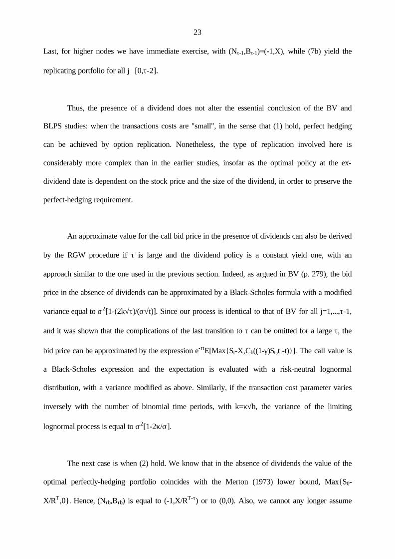
Last, for higher nodes we have immediate exercise, with (Nτ-1,Bτ-1)=(-1,X), while (7b) yield the
replicating portfolio for all j∈[0,τ-2].
Thus, the presence of a dividend does not alter the essential conclusion of the BV and
BLPS studies: when the transactions costs are "small", in the sense that (1) hold, perfect hedging
can be achieved by option replication. Nonetheless, the type of replication involved here is
considerably more complex than in the earlier studies, insofar as the optimal policy at the ex-
dividend date is dependent on the stock price and the size of the dividend, in order to preserve the
perfect-hedging requirement.
An approximate value for the call bid price in the presence of dividends can also be derived
by the RGW procedure if τ is large and the dividend policy is a constant yield one, with an
approach similar to the one used in the previous section. Indeed, as argued in BV (p. 279), the bid
price in the absence of dividends can be approximated by a Black-Scholes formula with a modified
variance equal to σ2[1-(2k√τ)/(σ√t)]. Since our process is identical to that of BV for all j=1,...,τ-1,
and it was shown that the complications of the last transition to τ can be omitted for a large τ, the
bid price can be approximated by the expression e-rtE[Max{St-X,Cb((1-γ)St,t1-t)}]. The call value is
a Black-Scholes expression and the expectation is evaluated with a risk-neutral lognormal
distribution, with a variance modified as above. Similarly, if the transaction cost parameter varies
inversely with the number of binomial time periods, with k=κ√h, the variance of the limiting
lognormal process is equal to σ2[1-2κ/σ].
The next case is when (2) hold. We know that in the absence of dividends the value of the
optimal perfectly-hedging portfolio coincides with the Merton (1973) lower bound, Max{S0-
X/RT ,0}. Hence, (Nτb,Bτb) is equal to (-1,X/RT-τ) or to (0,0). Also, we cannot any longer assume

24
that at time τ the intermediary will choose either to exercise the option, or to restructure the hedging
portfolio to the (Nτb,Bτb) that corresponds to a starting price Sτ-D, since the optimal hedging
portfolio is no longer independent of Nτ-1. The solution of this case is rather complex, but the
ultimate result turns out to be not very useful. It is expressed by Theorem 4, whose proof is
available from the authors on request.
Theorem 4. When both (2) and (9) hold the bid price of the call option in the presence of dividends
is equal to either Max{0,S0-X/Rτ} or to Max{0,S0-X/RT-D/Rτ}, depending on which one of the
second terms within braces is largest.
Theorem 4 basically implies that the bid price in the presence of a dividend is also equal to
the Merton bound under either immediate or defered exercise policy, whichever is largest. This is
the result that emerges when transaction costs become “too large” with respect to the binomial
parameters. It forms the counterpart of the result of Soner et al (1995) for the long call, and PL for
the short call when there are no dividends. Hence, the validity of relations (1) and (9) becomes
crucial in assessing the significance of the various theorems proved in this paper. Given their
importance, these relations will be discussed in the next section.
V. Extensions, Discussion, and Numerical Examples
All the results derived in this paper relied on the properties of the functions Cm(S0), Cm+(S0),
Cm-(S0), m=a,b, derived in Lemmas 1-3. It is the convexity of these functions and the size of their
derivatives that establish the key configuration of the early exercise boundary shown in Figure 1.
These properties also play a major role in the proofs of Theorems 1-3.

25
For this reason the extension of the above results to more than one dividend to expiration is
immediate and does not require a new formulation. It suffices to show that Lemmas 1-3 also hold
for the functions Cmd(S0), Cmd+(S0), Cmd-(S0), m=a,b, the option ask and bid prices when there is one
ex-dividend date prior to expiration. The proof relies on the solution of the systems (10a,b) and
(11a,b) for the long call ((15a,b) and (16a,b) for the short call) at τ-1, and the corresponding
relations (7a,b) for all times j∈[0,τ-1), and is otherwise identical to that of Lemmas 1-3. Hence, the
algorithms derived in Theorems 1 and 3 are also valid recursively for any number of dividends till
option expiration.
The inequality relations (1) are discussed at length in PL, where it is shown that for a
constant k they are satisfied only for small sizes of the binomial tree when u, d and R follow the
expressions that tend to diffusion. In other words, under (12) both τ and T-τ must be “small” for (1)
to hold.
Inequality set (9), though, is considerably more plausible, even for a constant k. Indeed,
consider the following parameter values17: σ=0.2, r=0.1, d=u-1, k=0.5%. Assume a dividend yield
D/Sτ≤0.1, and consider values of t/τ satisfying (9). It can be easily seen that with these parameter
values (9) is satisfied whenever √t/τ exceeds 0.00251, or whenever τ<39,500 price changes per
quarter. This works out to more than one price change per minute, corresponding to binomial tree
sizes far above those used in most practical applications.
Hence, as τ increases for a fixed k we have the following successive regimes: a) (1) and (9)
hold; b) (9) holds, but neither (1) nor (2) hold; c) both (2) and (9) hold; d) (2) holds but (9) is
violated. In the absence of dividends (9) is irrelevant, and the optimal portfolios are found by

26
relations (7a) for the ask price in all cases, while for the bid price they are given by relations (7b)
under regime (a), by the Merton bound under regime (c), and by one or the other of these two
alternatives under regime (b)18. In the presence of dividends Theorems 1 and 2 are valid under
regimes (a), (b) and (c), Theorem 3 holds under regime (a) and Theorem 4 under regime (c), while
one or the other may hold under regime (b).
Last, under regime (d), if (9) is not satisfied, then the general approach of this paper
continues to be valid, but none of the proofs of the theorems presented in this paper holds19.
Restructuring optimally the hedge portfolio for both long and short calls may now yield results that
have stockholdings lying outside the respective intervals [0,1] and [-1,0]. While it would still be
possible to derive results for such a case, the violation of (9) is, in our opinion, too rare an event to
make it worth the effort.
We provide below some perfectly-hedged option bid and ask prices when there is one
dividend prior to expiration, first for a fixed transaction cost parameter and a constant dividend, and
then for a proportional dividend and a parameter k declining in proportion to the size of the
binomial tree according to the Henrotte-Flesaker and Hughston assumption. The following
parameter values were kept constant in all results: S=$100; t1=0.25; t=t1/2; σ=0.2; r=0.1. For the
constant k and D in Table 1 T is 40, D=$5 and k=0.5%. With the chosen values of the other
parameters k=0.5% corresponds to the case where the inequalities (1) are satisfied. In our working
paper (Perrakis and Lefoll, 1997b) results are also provided for k=2.5%, when condition (2) is
satisfied and the bid prices are equal to the Merton bound.
In Table 1 the columns CaB and CbB indicate the ask and bid prices under the Black (1975)
assumption, as the maximum (for the ask) and the minimum (for the bid) of the call prices under

27
early and deferred exercise for all stock prices at ex-dividend date20. The entry ∆Cd is the difference
(Cad-Cbd) as percentage of the midpoint (Cad+Cbd)/2. The value-added of the new results presented
in this paper consists of the comparison of Cad (Cbd) to CaB (CbB).
As seen in the table below, and as expected from the computational algorithm, the
introduction of dividends raises substantially in all cases the correct ask price Cad in comparison
with the pseudo-American such price CaB. The increase is most significant when the option is at- or
slightly in-the-money. This rise, however, does not necessarily result in a wider bid/ask spread,
because the bid price Cbd rises even more than the ask price with respect to its pseudo-American
value. Similarly, Table 1 shows that when (1) holds the pseudo-American bid/ask spread is almost
always larger in both absolute and percentage terms than the correct spread. In other words, the
presence of dividends when transactions costs are not very large raises the bid price more than the
ask price, thus reducing the spread.
Table 1: Bid and ask call prices and spreads for T=40, k=.5%
Table 2, presents the ask and bid prices Cad and Cbd computed under our algorithm with a
transaction cost parameter k=κ√t1/T, under the Henrotte-Flesaker and Hughston assumption. These
values are then compared in Table 3 to the call prices of a conventional binomial model with
dividends, with k=0 but with modified volatilities equal to σ√(1+2κ/σ) and σ√(1-2κ/σ) for the ask
and the bid respectively. The dividend policy here is of the constant yield type21 with γ=5% and κ
was set equal to 0.5%; the remaining parameters are as in Table 1. Hence, the limiting case of k=0
and modified volatilities yields prices Cad and Cbd with respective volatilities equal to 0.2√1.05 and
0.2√0.95.

28
Table 2: Bid and ask call prices for k=κ√t1/T
Table 3: Bid and ask call prices for k=0, σ=0.2√1.05 and σ=0.2√.95
It is clear that the entries in Tables 2 and 3 are very close to each other, generally within
$.01 for both bid and ask. Further, there is a clear convergence to a value representing the
continuous-time limit as the number of time subdivisions increases, with the limit essentially
reached for T=50 (see note 12). Such convergence was also observed in all our other simulation
results (not reported here but available on request), in which σ was varied between 0.10 and 0.30,
and T was varied between 0.10 and 0.40. Hence, our algorithms represent the appropriate
generalization of the binomial model for American options in the presence of dividends and
transaction costs under the perfect hedging assumption.
VI. Conclusions
This paper has presented a procedure for the computation of the perfectly-hedged bid and
ask prices for an option on an asset with physical delivery when there are known dividends prior to
expiration. The computational algorithms extended previous studies by Boyle and Vorst (1992),
Bensaid et al (1992) and Perrakis and Lefoll (1997a). It was shown that the optimal perfect hedging
policy corresponded to a form of replication, somewhat more complex than the usual replication of
the positions of the two successor nodes of the binomial tree. This replication was always optimal
for the ask price, but it was optimal for the bid price only if the key inequality set (1) held.

29
The results were conditional on the key inequality set (9), containing restrictions on the
binomial, transaction cost parameters, and dividend yield at the ex-dividend dates. These
restrictions are weaker than the inequality set (1), which must be satisfied for the bid price to have a
non-trivial value. Both (1) and (9) are usually satisfied if the dividend policy is of the constant yield
type at ex-dividend date, and if the transaction cost parameter declines in proportion to the square
root of the number of time periods. In such a case both ask and bid prices reach continuous-time
limits with modified volatilities.
The results of this paper are for options with physical delivery of the underlying asset. An
important extension in future research would be to cash-settlement options, such as index options.

30
Appendix
Proof of Lemmas 1, 2 and 3.
All proofs use induction on n. For n=1 Lemmas 1 and 2 clearly hold, while for Lemma 3
the proof is virtually identical for all four functions; we shall present it in detail for the last two.
For n=1 the replicating portfolio (N0b,B0b) is equal to (-1,X/R), or to (0,0) when both S0u and
S0d are on the same side of X/(1-k). Assume that X/(1-k)∈(S0d,S0u); then the solution of system
(7b) yields a replicating portfolio -NobS0=[S0u(1-k)-X]/[u(1-k)-d(1+k)], B0b=-N0bS0d(1+k)/R,
and by (1) it is clear that all parts of the lemma hold22 for both functions for n=1, QED.
Next comes the convexity proof, which is identical for all functions in Lemmas 1-3, and
will again be carried out for the last two functions of Lemma 3. Assume that convexity holds for
both replicating portfolios (Nji,Bji), i=1,2, at time j and at nodes uSj and dSj respectively. Solving
the system (7b) and re-arranging, we get the replicating portfolio (Nj,Bj) at node Sj, which yields
-[(1-k)NjSj+Bj]=-{α[Nj1u(1-k)Sj+Bj1]+(1-α)[Nj2d(1+k)Sj+Bj2]}/R, where α≡[R(1-k)-d(1+k)]/
[u(1-k)-d(1+k)]∈[0,1]. By the induction hypothesis both terms in brackets are non-negative,
non-decreasing and convex in uSj and dSj, implying that their convex combination is also
convex in Sj; similar expressions hold for -[(1+k)NjSj+Bj], QED.
The proof for the other two functions of Lemma 3 involving the ask price replicating
portfolios, and for the functions Ca(S0,n) and Cb(S0,n) of Lemmas 1 and 2 is identical. Convexity
is also sufficient for the proof of the derivative conditions in Lemmas 1 and 2, since when the
option is always in-the-money both Ca and Cb are equal to S0-X/Rn. Finally, the last part of
Lemma 2 is a straightforward application of Lemma 2 of BLPS, QED.

31
It remains now to show that N(S0) is non-decreasing and B(S0) is non-increasing for both
ask and bid prices. Since the proof is identical, we present it only for the ask price and omit the
subscripts for simplicity of presentation. Solving (7a) we find that N(S)∼[C+(Su)-C-(Sd)]/S. By
the induction hypothesis N(dS) is non-decreasing in dS. Rewriting C+(Su)-C-(Sd) =[C+(Su)-
C+(Sd)]+[C+(Sd)-C-(Sd)] and dividing both of them by S, we observe that both are non-
decreasing: the second one is proportional to N(dS) and the first one to [C+(Su)-C+(Sd)]/[S(u-
d)], with the latter being non-decreasing by the convexity of the C+ function, QED.
The proof for B(S0) is similarly based on the convexity proven in the first part. From (7a)
we have B(S)∼u(1+k)C-(Sd)-d(1-k)C+(Su). Letting a prime denote the derivative, we have by
induction that B’(Sd) and B’(Su) are negative. Hence, B’(S)<0⇔(1+k)C-’(Sd)<(1-k)C+’(Su).
The right-hand-side (RHS) exceeds (1-k)(1+k)C’(Su), while C-’(Sd) is less than (1-k)C’(Sd),
thus reducing the relation to C’(Sd)<C’(Su), which obviously holds, QED.
Proof of Theorem 1.
Theorem 1 corresponds to Theorems 1 and 2 of our working paper (Perrakis and Lefoll,
1997b). Only a summary of the proofs of these two theorems will be given here. We first show
that the optimal stockholdings Nτ-1* at any node are in the interval [0,1]. At j=τ-1 we derive Qτ-
1(Nτ-2, Sτ-1) by solving the program (4) subject to (5), where the functions Qτ(Nτ-1,uSτ-1) and
Qτ(Nτ-1, dSτ-1) are given by the appropriate expressions in the RHS of (8a,b,c). We need to show
that Qτ(0,uSτ-1)≥Qτ(0,dSτ-1) and Qτ(1,uSτ-1)≤Qτ(1,dSτ-1), since we know that Nτa∈[0,1] always.
In such a case the slope of the binding constraint as a function of Nτ-1 in (5) would be either
-uSτ-1(1+k) or -uSτ-1(1+k)+Dk for Nτ-1=0-, both of which are less than -R(1+k)Sτ-1 in view of
(9), thus yielding an Nτ-1* that is ≥0 for all Nτ-2≤0; similarly, the slope at Nτ-1=1+ would be

32
greater than -R(1-k)Sτ-1, yielding Nτ-1*≤1. The demonstration relies heavily on the convexity
results of Lemmas 1, 2 and 3 and is straightforward but tedious because of the various cases
arising out of the different intervals of Sτ; it will be omitted.
Next we want to show that at time τ-1 the conditions of Theorem 3 of BLPS hold for the
unique optimal portfolio (Nτ-1*,Bτ-1*), since under these conditions program (4)-(6) yields a
unique replicating portfolio for all j∈[0,τ-1]. Hence, we must show that the convex functions
Qτ(Nτ-1,uSτ-1) and Qτ(Nτ-1,dSτ-1) intersect at a single value of Nτ-1, which defines (Nτ-1*,Bτ-1*).
We also have to show that Nτ-1* is non-decreasing and Bτ-1* is non-increasing in Sτ-1, and that
the optimal portfolios at any two successive values of Sτ-1 satisfy a certain technical condition
(condition (6) of BLPS). It suffices to provide the proof for points Sτ∈(Sτ1,Sτ2) or Sτ∈(Sτ3,∞),
since this is the most general case.
Consider two consecutive points A and B at τ-1 and their successor points l=1,2,3 in the
binomial tree, as in Figure A1(a), and let Sl denote the value of Sτ at point l, with the Sl's lying in
the indicated intervals. As argued above, Qτ(0,S1)≥Qτ(0,S2)≥Qτ(0,S3), with the inequalities
holding strictly for the interval of values of Sτ that we are considering. The constraints (8a,b,c)
define functions Qτ(Nτ-1,Sτ) that have the piecewise linear forms shown in Figure A1(bc), with
the slope of the steeper line(s) being -(1+k)Sτ or -(1+k)Sτ+kD, that of the flatter line
-(1-k)Sτ-kD, and with the last kink at a value of Nτ-1 that is greater than or equal to the
corresponding stockholding Nτa. Our theorem is easily seen to hold if it can be shown that
the functions Qτ(Nτ-1,uSτ-1) and Qτ(Nτ-1,dSτ-1) intersect at a single value of Nτ-1, defined by
the steeper line(s) of the u-function and the flattest line of the d-function, as in Figure A1(d).
By (9) that value would be Nτ-1*, the optimal Nτ-1 in the minimization problem (4) subject to (5),

33
and it would lie between the stockholdings Nτa corresponding to the successor u- and d-nodes in
the binomial tree. Further, the sequence of portfolios (Nτ-1*, Bτ-1*) along the successive nodes A
and B of the binomial tree at time τ-1 would satisfy the conditions of the BLPS Theorem 3.
Indeed, it is clear from Figure A1(d) that Nτ-1*(A)≥Nτ-1*(B), Bτ-1*(A) ≤Bτ-1*(B), while
condition (6) of Theorem 3 of BLPS corresponds to d(1-k) ≤R[Bτ-1*(B)-Bτ-1*(A)]/SA[Nτ-1*(A)-
Nτ-1*(B)]≤u(1+k). It is clearly satisfied, since the slope of the line BA in Figure A1(d) lies
between the two lines that bracket it to the left of point A, and whose slopes are -SAd(1-k)-kD
and -SAu(1+k)+kD.
Figure A1
The most general case is when both Qτ(Nτ-1,uSτ-1) and Qτ(Nτ-1, dSτ-1) are given by (8c),
ie. are both equal to Max {Wa( Nτ-1, Sτ), Wb ( Nτ-1, Sτ)}. For Nτ-1 ∈ [0,1] Wa (Nτ-1, uSτ-1)
≥ Wb(Nτ-1,dSτ-1), with the two functions being equal to -X at Nτ-1=1, and the inequality being
strict for Nτ-1∈[0,1). It suffices, therefore, to show that the steepest part of Wb(Nτ-1,uSτ-1)
intersects with the flattest part of Wb(Nτ-1,dSτ-1), as in Figure A1(d). Since Nτa(u)≥Nτa(d) and
Bτa(u)≤Bτa(d), it suffices to show that Wb(Nτa(d),uSτ-1)≥Wb(Nτa(d),dSτ-1), and/or that
Wb(Nτa(u),dSτ-1)≥Wb(Nτa(u),uSτ-1). The proof is again straightforward and will be omitted; it
uses induction on T-τ, as well as the convexity results of Lemma 3.
Proof of Theorem 2.
As shown in BV pp. 274-276, the evaluation of the replicating portfolio in the absence of
dividends corresponds to the discounted expectation of the call option value at expiration under

34
a modified Markovian process, in which the transition probabilities depend on the previous
move. Adopting similar notation to BV, we set these transition probabilities in matrix form P,
where:
and u =u(1+k), d =d(1-k); the initial transition takes place with probabilities p and 1-p for up
and down moves, where p=[R-d ]/[ u -d ]. In (A1) pu and pd are the probabilities of an up move,
given that the previous move was, respectively, an up and a down move. The Markovian process
consists of a sequence of random variables x1,...,xτ, each one of which can have only two states
with values lnu and lnd. The stock price Sτ is equal to S0eY, where Y=Σxj. Let also Yτ-1=
x1+...+xτ-1, and Y1=Max{Yτ-1:Yτ-1≤ln(Sτ-1,1/S0)}, Y2=Min{Yτ-1:Yτ-1≥ln(Sτ-1,2/S0)}.
In our case the Markovian process is identical to that of BV for all j=1,..,τ-1. At τ-1,
however, the matrix of transition probabilities will change depending on the value of Yτ-1.
Setting D=γSτ, we note that for Yτ-1≤Y1 and Yτ-1∈(Y1,Y2) the matrix P must be replaced by P1
and P2 respectively23, where:
(A2) P1=
p-1p-1
pp
du
du, P2=
′′
′′
p-1p-1
pp
du
du,
and pu=[R(1+k)- d ]/[u(1+k)-d(1-k)], pu'=[R(1+k)- d ]/[u -d(1-k)], k≡k(1-γ), while pd, pd' simply
replace R(1+k) by R(1-k) in the numerators. As for the terminal positions at τ, they correspond,
],d-u/[]d-k)-[R(1=p ],d-u/[]d-k)+[R(1=p ,p-1p-1
ppP )1A( du
du
du
≡

35
as argued earlier, to immediate or deferred exercise for Sτ-1 outside the interval (Sτ-1,1,Sτ-1.2), and
to immediate exercise for an up move and deferred exercise for a down move otherwise.
Analytically, therefore, the option ask price Cad is given by an expectation with respect to the
adjusted process, in an expression similar to (10) of BV:
(A3) Cad=R-τE{Max[(1+xτk)S0eY-X,Bτa+(1+xτk)NτaS0(1-γ)eY]},
where xτ=1 if xτ=lnu and xτ=-1 if xτ=lnd, and the adjusted process is identical to the one
described in BV except when the logarithmic returns Yτ-1 are such that Yτ-1≤Y1 and
Yτ-1∈(Y1,Y2), when the matrix P is replaced by P1 and P2 respectively.
For the limiting process we consider the binomial model given by (12) and we assume
t=1 for simplicity. We then examine the limiting value of (A3) when τ becomes large. For k=0
expression (A3) becomes the value of an American call option with a single proportional
dividend payable at τ under the binomial model. To prove the theorem we first show that for a
large τ an approximate limiting lognormal distribution of the stock price Sτ exists under our
process, similar to the limiting distribution of (12) but incorporating the transactions costs. The
following result allows us to use directly the derivations of the no-dividend case, as in BV,
pp.276-278.
Lemma 4. The random variable Y=x1+...+xτ of expression (13) has the same asymptotic
behaviour for large τ and small k as the corresponding random variable Y of the no-dividend
case, with:
(A4) E(Y)=r-Var(Y)/2 + O(1/√τ) +O(k2), Var(Y)=σ2{1 + O(k2) + [2k/σ + O(k3)]√τ} + O(1/√τ).

36
Proof. Let Y denote the random variable of the no-dividend case (the Y of the BV study).
Clearly, since Y=Yτ-1+xτ, Y and Y differ only insofar as the last step xτ takes place with
transition matrix P1, P2 or P depending on the value of Yτ-1, instead of P always. Rewriting
pu=[R(1+k)-d(1-k)]/[u(1+k)-d(1-k)-γk(u+d)] and expanding u+d=2[1+σ2(1/τ)/2+O(τ-3/2)], we
can rewrite pu as [R(1+k)-d(1-k)][u(1+k)-d(1-k)-γk(u+d)]/[[u(1+k)-d(1-k)]2-O(k2)-O(k/τ)],
which implies that pu≈pu[1+2kγ/[u(1+k)-d(1-k)]+O(1/τ)]=pu(1+λ1). Expanding the u and d terms
in the denominator of λ1, we find that λ1=[γk+O(1/τ)]/[k+σ√1/τ+O(1/τ)] ≈γk/[k+σ√1/τ], which
is <γ. Similarly, we have pd=pd(1+λ1), while pu'=[R(1+k)-d(1-k)]/[u(1+k)-d(1-k)-γkd].
Expanding d in the term γkd in the denominator and following the same procedure as with pu,
we get pu'≈pu(1+λ2), where λ2=γk/[2(k+(1+k)σ√1/τ)]<λ1/2; similarly, pd'≈pd(1+λ2).
To find E(Y) and Var(Y) we replace pu and pu' by their asymptotic approximations into
the transition matrices P1 and P2 and consider the distributions of Y and Y. Since Yτ-1 is
common to both these random variables, which differ only whenever Yτ-1<Y2, we consider the
following events i=1,...,6, with corresponding probabilities π i and expectations Ei≡E[Yτ-1� event
i occurs]: {Yτ-1≤Y1, last event at τ-1 is an up move}; {Yτ-1≤Y1, last event at τ-1 is a down
move}; {Yτ-1∈(Y1,Y2), last event at τ-1 is an up move}; {Yτ-1∈(Y1,Y2), last event at τ-1 is a
down move}; {Yτ-1≥Y2, last event at τ-1 is an up move}; {Yτ-1≥Y2, last event at τ-1 is a down
move}. Let also E≡E(Yτ-1). Then we have:
(A5) E(Y) =E+(π1+π3+π5)[pulnu+(1-pu)lnd]+(π2+π4+π6)[pdlnu+(1-pd)lnd]
+λ1(lnu-lnd)(π1pu+π2pd)+λ2(lnu-lnd)(π3pu+π4pd)
=E(Y)+2σ√1/τ[λ1(π1pu+π2pd)+λ2(π3pu+π4pd)].
37
Since the last term in the RHS of (A5) is clearly O(1/√τ), the first part of our Lemma 4 follows
directly from Lemma 2 of BV, QED.
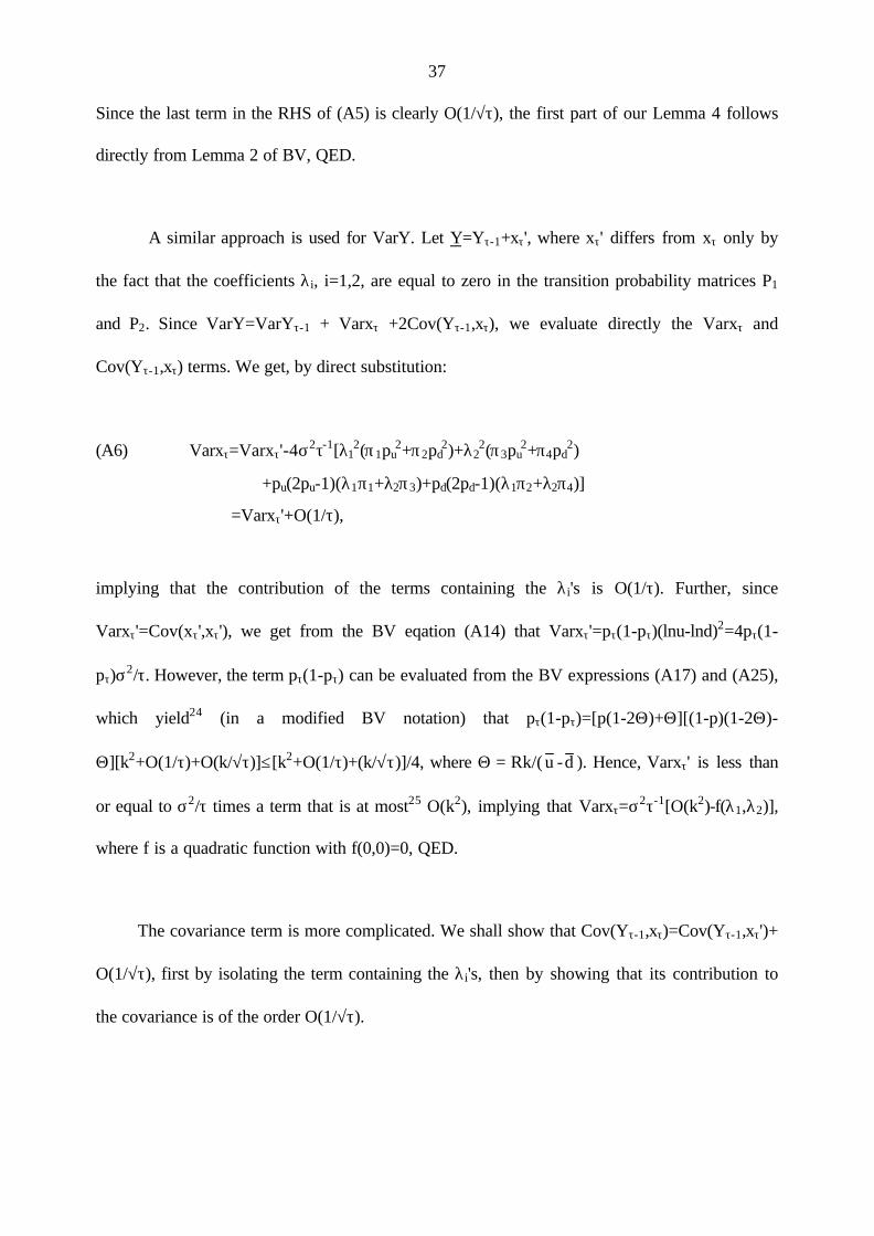
A similar approach is used for VarY. Let Y=Yτ-1+xτ', where xτ' differs from xτ only by
the fact that the coefficients λi, i=1,2, are equal to zero in the transition probability matrices P1
and P2. Since VarY=VarYτ-1 + Varxτ +2Cov(Yτ-1,xτ), we evaluate directly the Varxτ and
Cov(Yτ-1,xτ) terms. We get, by direct substitution:
(A6) Varxτ=Varxτ'-4σ2τ-1[λ12(π1pu
2+π2pd2)+λ2
2(π3pu2+π4pd
2)
+pu(2pu-1)(λ1π1+λ2π3)+pd(2pd-1)(λ1π2+λ2π4)]
=Varxτ'+O(1/τ),
implying that the contribution of the terms containing the λi's is O(1/τ). Further, since
Varxτ'=Cov(xτ',xτ'), we get from the BV eqation (A14) that Varxτ'=pτ(1-pτ)(lnu-lnd)2=4pτ(1-
pτ)σ2/τ. However, the term pτ(1-pτ) can be evaluated from the BV expressions (A17) and (A25),
which yield24 (in a modified BV notation) that pτ(1-pτ)=[p(1-2Θ)+Θ][(1-p)(1-2Θ)-
Θ][k2+O(1/τ)+O(k/√τ)]≤[k2+O(1/τ)+(k/√τ)]/4, where Θ = Rk/( u -d ). Hence, Varxτ' is less than
or equal to σ2/τ times a term that is at most25 O(k2), implying that Varxτ=σ2τ-1[O(k2)-f(λ1,λ2)],
where f is a quadratic function with f(0,0)=0, QED.
The covariance term is more complicated. We shall show that Cov(Yτ-1,xτ)=Cov(Yτ-1,xτ')+
O(1/√τ), first by isolating the term containing the λi's, then by showing that its contribution to
the covariance is of the order O(1/√τ).

38
We first observe that inequality (9) implies that γk is less than a term that is O(1/√τ).
Under the constant dividend yield assumption (9) takes the form u(1+k)>R(1+k), R(1-k)>d(1-k),
where k=k(1-γ). Expanding the first of these inequalities we get γk(1+σ/√τ)<(1+k)σ/√τ +O(1/τ),
or γk<(1+k)σ/√τ=O(1/√τ). Hence, γk is O(1/√τ), a fact that will be used in the subsequent proof.
Evaluating the Cov(Yτ-1,xτ) directly, we get, after replacing lnu and lnd,
(A7) Cov(Yτ-1,xτ)=Cov(Yτ-1,xτ')+2{λ1[puπ1(E1-E)+pdπ2(E2-E)]
+λ2[puπ3(E3-E)+pdπ4(E4-E)]}σ/√τ
=Cov(Yτ-1,xτ')+2Aσ/√τ ,
where A is a linear function of λ1 and λ2, of the type λ1α+λ2ß. We want to show that 2Aσ/√τ is
O(1/√τ) with the same degree of precision as in BV. By the Schwartz inequality we have
Cov2(Yτ-1,xτ)≤VarYτ-1Varxτ. Since VarYτ-1=σ2(1+2k√(τ-1)/σ)+O(1/√τ)+O(k2) and Varxτ is at
most equal to σ2τ-1[O(k2)-f(λ1,λ2)], we get from this inequality that Cov2(Yτ-1,xτ) is less than or
equal to [σ4τ-1+2kσ3√(1-τ-1)/√τ][O(k2)-f(λ1,λ2)] plus terms of order higher than 1/τ. All the
terms in this last expression are at most O(1/τ), given that kf(λ1,λ2) is at most O(1/√τ) since
kλ1<γk=O(1/√τ). Hence, Cov(Yτ-1,xτ) is at most O(1/√τ), QED.
The last step is to show that Cov(Yτ-1,xτ') is O(1/√τ), in which case (A7) implies that
2Aσ/√τ will also be O(1/√τ). Replacing Yτ-1 by the sum Σxi, we find that Cov(Yτ-1,xτ')=
ΣCov(xτ-i,xτ'). Evaluating the terms in the sum on the basis of the BV relation (A14) (p. 287) we
find that, in that study's notation,
(A8) ΣCov(xτ-i,xτ')=Σpτ-i(1-pτ-i)Θi2i(lnu-lnd)2≤(1/4)ΣΘi2i(4σ2/τ),

39
where we have used relation (A17) of BV. Since ΣΘi2i=[2Θ-(2Θ)τ]/[1-2Θ], we can neglect the
factor (2Θ)τ, as in BV p. 290. Similarly, replacing 2Θ/[1-2Θ] into the RHS of (A8) by its
asymptotic value √τ[k/2σ+O(1/√τ)] (from (A23) of BV), we find that Cov(Yτ-1,xτ') is O(1/√τ),
QED.
This key result allows us now to employ the same technique as in BV in finding the
asymptotic properties of the RHS of (A3). It implies that for large τ and small k the factor xτ in
expression (A3) can be neglected, implying that Cad can be approximated by expression (13). As
argued in BV (p. 277) the distribution of Y for large τ tends to the normal with mean and
variance given by (A4); hence, the distribution of Sτ tends to the corresponding lognormal
distribution. Similarly, if the number of periods T-τ from ex-dividend date to option expiration
is also large then the term Bτa+Nτa(1-γ)S0eY would tend to a Black-Scholes call option value with
variance σ2[1 + (2k√T-τ)/(σ√t-t1)]. Theorem 2 now follows by using the standard RGW
approach in order to evaluate the limiting form of (13).
Proof of Theorem 3.
The main task is to show that such a portfolio exists and is the optimal hedging portfolio
at time τ-1, since this would restore the convexity in Nj of the constraints (5) for all j≤τ-2. The
key to the proof is the form of the constraint (14a) when at least one of the points uSτ-1 and dSτ-1
lies within the indicated interval. There are many possibilities; only the most important or
difficult to prove will be covered here. By Lemma 2 Nτb∈[-1,0], implying that the slopes of both
constraints in (14a) are -Sτ(1+k) and -(1+k)Sτ+Dk for Nτ-1≤-1, and -(1-k)Sτ and -(1-k)Sτ-Dk for
Nτ-1≥0. By (1) and (9) Nτ-1*, the optimal Nτ-1, will lie within the interval [-1,0] if it can be shown

40
that it is the u-and d-branches of the constraints at the RHS of (14a) that bind respectively at Nτ-1
= -1 and Nτ-1=0.
If Nτb=-1 then for Nτ-1=-1 it is the relative sizes of X and X/RT-τ+D that will determine
whether it is the first or the second term in braces in the RHS of (14a) that binds. It will be
assumed that we are in the situation shown in Figure 1, with X/(1-k)<X/RT-τ+D, which is the
most complex; in such a case we have -1<Nτb(u)<Nτb(d)≤0 for Sτ within the interval indicated in
(14a). Consider first the case where the second terms in the RHS of (14a) bind at both u- and d-
branches. For Nτ-1=-1 the u-branch lies above the d-branch if (1+k)(u-d)Sτ-1>
∆Bτb+(1+k)∆Nτb(Sτ-D), where ∆Bτb≡Bτb(d)-Bτb(u) and ∆Nτb(Sτ-D)≡Nτb(d)(dSτ-1-D)-Nτb(u)(uSτ-1-
D); this inequality holds by the convexities shown in Lemma 3. Similarly, at Nτ-1=0 ∆Bτb+(1-
k)∆Nτb(Sτ-D)>0 by Lemma 3. The constraints in (14a) become then convex, implying by (1) and
(9) that they have a unique intersection, which defines Nτ-1*, QED.
Similarly, if it is the first term in (14a) that binds in both branches the d-branch is
dominant for all Nτ-1∈(-1,0) and the u-branch for Nτ-1≤-1, implying that Nτ-1*=-1. Note that,
since the slope of the first term exceeds both slopes of the second term in (14a), we only need to
compare the second terms in both branches if the second term in the u-branch is ≤X at Nτ-1=-1.
For D=0 it was already known from BV and BLPS that the optimal perfectly hedging
portfolio is a replicating one given by (7b). This implies that for D=0 the constraints in (14a)
intersect as in Figure A2: the portfolio is defined by point Ñ, where the flattest part of the u-
branch intersects with the steepest part of the d-branch. This type of intersection is also
preserved when D is >0 but (1) and (9) hold, as it can be easily shown by induction on T-τ. This
point is also the optimal portfolio (Nτ-1*,Bτ-1*) when it is not restricted by the immediate

41
exercise constraint, as in Figure A2. In this case the lack of convexity of the constraints in the
RHS of (14a) does not prevent the existence of a single replicating portfolio corresponding to
deferred exercise and given by (15a,b).
By contrast, in the situation depicted in Figure A3 the portfolio at Ñ is infeasible since it
lies above the immediate exercise constraint for the u-branch. Hence, the optimal hedging
portfolio corresponds to a portfolio replicating immediate exercise for an up move and deferred
exercise for a down move. This portfolio is given by (16a,b). The optimality of the solutions of
both (15a,b) and (16a,b) comes from an application of the program (4)-(6), in conjunction with
inequalities (1) and (9) on the slopes of the constraints in Figures A2 and A3. Last, we have
Nτ-1*=-1, Bτ-1*=X when the immediate exercise constraint intersects the vertical axis below the
point A in Figure A3.
It was thus shown that replication is optimal at τ-1. It is also easy to show that the
optimal portfolio (Nτ-1*,Bτ-1*) along the successive nodes of the binomial tree satisfies the
conditions for the optimality of replication of the BLPS Theorem 3, as with the long call. This
completes the proof of the theorem.
Figure A2
Figure A3

42
References
Bensaïd, B., J. P. Lesne, H. Pagès, and J. Scheinkman, 1992, Derivative asset pricing withtransaction costs, Mathematical Finance 2, 63-86.
Black, F., 1975, Fact and fantasy in the use of options, Financial Analysts Journal 31, 36-41, 61-72.
Black, F. and M. Scholes, 1973, The pricing of options and corporate liabilities, Journal of PoliticalEconomy 81, 637-659.
Boyle, P. P. and T. Vorst, 1992, Option replication in discrete time with transactions costs, Journalof Finance 47, 271-293.
Constantinides, G., 1986, Capital market equilibrium with transactions costs, Journal of PoliticalEconomy 94, 842-862.
Cox, J. C., S. Ross and M. Rubinstein, 1979, Option pricing: A simplified approach, Journal ofFinancial Economics 7, 229-263.
Cox, J. C. and M. Rubinstein, 1985, Options markets (Prentice Hall, Englewood Cliffs).
Davis, M. H. A., V. G. Panas, and T. Zariphopoulou, 1993, European option pricing withtransaction costs, SIAM Journal of Control and Optimization 31, 470-493.
Dumas, B. and E. Luciano, 1991, An exact solution to a dynamic portfolio choice problem undertransactions costs, Journal of Finance 46, 577-595.
Edirisinghe, C., Naik, V., and Uppal, R., 1993, Optimal replication of options with transaction costsand trading restrictions, Journal of Financial and Quantitative Analysis 28, 117-138.
Flesaker, B. and L. P. Hughston, 1994, Contingent claim replication in continuous time withtransaction costs, Working paper (Merrill Lynch).
Geske, R., 1979, A note on an analytical formula for unprotected american call options on stockswith known dividends, Journal of Financial Economics 7, 375-380.
Henrotte, P., 1993, Transactions costs and duplication strategies, Working paper (Graduate Schoolof Business, Stanford University).
Hodges, S. and A. Neuberger, 1989, Optimal replication of contingent claims under transactionscosts, Review of Futures Markets 8, 222-242.
Hull, J. C., 1997, Options, futures, and other derivatives (Prentice-Hall, Englewood Cliffs).
Jarrow, R. and S. Turnbull, 1996, Derivative securities (Southwestern, Cincinnati).
Lefoll, J. and S. Perrakis, 1995, Transactions costs and option bid-and-ask spread on the SwissOptions and Financial Futures Exchange (SOFFEX), Canadian Journal of Administrative Sciences12, 276-289.
43
Leland, H., 1985, Option pricing and replication with transactions costs, Journal of Finance 40,1283-1301.
Merton, R.C., 1973, Theory of rational option pricing, Bell Journal of Economics and ManagementScience 4, 141-183.
Merton, R.C., 1989, On the Application of the continuous-time theory of finance to financialintermediation and insurance, The Geneva Papers on Risk and Insurance 14, 225-261.
Omberg, E., 1987, A note on the convergence of binomial-pricing and compound-option models,Journal of Finance 42, 463-469.
Perrakis, S. and J. Lefoll, 1997a, Derivative asset pricing with transactions costs: An extension,Computational Economics 10, 359-376.
Perrakis, S. and J. Lefoll, 1997b, Option pricing and replication with transaction costs anddividends, Working paper 97.02 (International Finance Laboratory, Université de Genève).
Rendleman, R. and B. Bartler, 1979, Two-state option pricing, Journal of Finance 34, 1093-1110.
Roll, R., 1977, An analytic valuation formula for unprotected american call options on stocks withknown dividends, Journal of Financial Economics 5, 251-258.
Selby, M. J. P. and S. D. Hodges, 1987, On the evaluation of compound options, ManagementScience 33, 347-355.
Soner, H. M., S. E. Shreve, and J. Cvitanic, 1995, There is no nontrivial hedging portfolio foroption pricing with transaction costs, Annals of Applied Probability 5, 327-355.
Whaley, R. E., 1981, On the valuation of american call options on stocks with known dividends,Journal of Financial Economics 9, 207-212.

44
Endnotes
1. In fact, the derived portfolios replicate exercise or deferral at the successor nodes. Nonetheless,
the super-replication approach is necessary in American options since the optimality of
replication is parameter-dependent, as we show in this paper. The difference between
replication and super-replication in the analytical structure of the model is shown in the next
section.
2. See BV for the ask, and PL for the bid.
3. It is assumed, following Roll (1977), that the dividend is paid with certainty at time τ no matter
what the price of the stock; hence, for large values of T and τ and low values of Sτ the dividend
policy must be of the constant yield or less. Further, it is assumed without loss of generality that
payment of the dividend does not alter the initial binomial process.
4. Our results can easily be extended without reformulation to the case where the ex-dividend
price is Sτ-δD, with 0<δ�1.
5. An additional requirement is that the terminal price must satisfy Sn∉[X/(1+k),X/(1-k)]. As
shown in PL, replication is still optimal when there is a value of Sn in the interval
[X/(1+k),X/(1-k)].
6. When the stock price is in the indicated interval, it is cheaper for an investor who wishes to own
stock to exercise the option, even though the stock price may be below the exercised price.

45
7. These properties were originally proven in Merton (1973). The properties of the replicating
portfolios (N0i,B0i), i=a,b, as functions of S0 are easily seen to hold; see, for instance, BV.
8. Although this case is a theoretical possibility, it did not appear in any one of our simulation
results. For the constant dividend yield case the second intersection point does not appear if
the dividend yield exceeds the transaction cost parameter k, as is usually the case.
9. Note that this portfolio is independent of the holdings (Nτ-1,Bτ-1).
10. This point is important and controversial. The optimal policy at each node is dependent on
the inherited amount of stock. If the two boundary values Nmin and Nmax were also dependent
on that inherited amount the dynamic programming algorithm presented by BLPS would
have become explosive very quickly, given the increase in the number of possible paths
throughout the binomial tree. An incorrect statement to that effect was made in a paper by
Edirisinghe et al (1993, p. 119). The proof for the independence is in the original BLPS
paper, as two of its co-authors showed us in a private communication. We are indebted to
Bernard Bensaïd and Jean-Philippe Lesne for pointing out to us this property of their
algorithm.
11. Theorem 1 corresponds to Theorems 1 and 2 in our working paper (Perrakis and Lefoll,
1997b). Theorem 1 demonstrates that the stockholdings in the optimal portfolio lie between
0 and 1, while Theorem 2 proves the replication result. Note that because of this Theorem 2
in this paper is Theorem 3 in the working paper, Theorem 3 is Theorem 4, etc.

46
12. Otherwise (9) will be violated for low values of Sτ-1. Our results are also valid for dividend
policies with D=γSτ for all Sτ below a certain limit, and D constant for higher Sτ‘s.
13. See, for instance Cox and Rubinstein (1985), p. 240.
14. This limit is reached under an oscillating pattern that precludes the estimation of the number
of subdivisions necessary to reach an accurate solution; see Omberg (1987). In practice,
most textbooks suggest that as few as 30 subdivisions may be enough for an acceptable
accuracy level in most applications. See Hull (1997, p. 348), and Jarrow and Turnbull (1996,
p. 328).
15. The Roll-Geske-Whaley procedure normally assumes a constant dividend, whose discounted
value is subtracted from the initial stock price S0. While this is a reasonable formulation in the
absence of transactions costs, it would lead to an underestimation of the magnitude of the costs
of hedging the intermediary's position, since the value of the stock does not include the
dividend.
16. Since the optimal policy turns out to be independent of the path of values of Sτ in Theorem 3,
we omit the argument ωτ hereafter. Recall also that relations (9) are automatically satisfied
when (1) holds.
17. The value of σ is the one used by BV, while the value of k represents the maximum bid-ask
spread for stock quotations found in the Swiss market by Lefoll and Perrakis (1995).
18. See PL.

47
19. See the proof of Theorem 1 in our working paper (Perrakis and Lefoll, 1997b). Note that for
a constant k and for such large values of τ relations (2) are expected to hold, and the bid
price would become equal to the Merton bound as in Theorem 4, while the ask price would
also become very large.
20. These are known as pseudo-American prices. They are computed under the assumption that
exercise occurs either at ex-dividend date or at expiration for all nodes of the binomial tree.
21. The results were very similar when a constant D=$5 was assumed.
22. The first function has slope u(1-k2)(R-d)/[R[u(1-k)-d(1+k)]], while the second's slope has
the same denominator but a numerator equal to u[R(1-k)2-d(1-k2)]; both expressions satisfy
the lemma, since they lie respectively in (0,1+k) and (0,1-k).
23. The proof is identical to the sequence followed in the BV derivation of their equations (7)
and (8), where the starting stock price is Sτ-2.
24. In this step, as well as in other parts of this proof, we make use of the fact that for any
q∈(0,m) we have q(m-q)≤m2/4≤1/4 if m<1; here we have q=p(1-2Θ)+Θ.
25. We assume, without loss of generality, that O(k2) tends to zero slower than O(k/√τ).

Table 1: Bid and ask call prices and spreads for T=40, k=.5%
X($) Cad($) Cbd($) CaB($) CbB($) ∆Cd(%)
85 16.270 16.056 16.128 13.336 1.33
90 11.928 11.134 11.503 8.978 6.89
95 8.295 6.493 7.679 5.350 24.37
100 5.509 3.050 5.255 2.381 57.46
105 3.517 1.265 3.444 0.558 94.21
110 2.175 0.465 2.158 0.048 129.50
115 1.296 0.150 1.294 0.004 158.63

Table 2: Bid and ask call prices for k=κ√t1/T
T=6 T=20 T=50 T=100 T=200
X Cad Cbd Cad Cbd Cad Cbd+ Cad Cbd Cad Cbd
85 16.136 16.132 16.124 16.109 16.122 16.107 16.122 16.107 16.122 16.107
90 11.457 11.408 11.501 11.447 11.502 11.448 11.501 11.449 11.499 11.446
95 7.616 7.513 7.492 7.396 7.529 7.429 7.515 7.417 7.516 7.417
100 4.588 4.494 4.517 4.400 4.529 4.409 4.522 4.398 4.519 4.394
105 2.394 2.284 2.524 2.413 2.529 2.416 2.533 2.417 2.536 2.419
110 1.283 0.573 1.320 1.231 1.338 1.246 1.343 1.251 1.346 1.253
115 0.556 0.000 0.647 0.567 0.669 0.604 0.675 0.609 0.678 0.611

Table 3: Bid and ask call prices for k=0, σ=0.2√1.05 and σ=0.2√.95
T=6 T=20 T=50 T=100 T=200
X Cad Cbc Cad Cbd Cad Cbd Cad Cbd Cad Cbd
85 16.141 16.121 16.125 16.108 16.121 16.106 16.123 16.106 16.124 16.104
90 11.454 11.408 11.501 11.447 11.504 11.446 11.506 11.444 11.504 11.433
95 7.621 7.503 7.499 7.377 7.539 7.418 7.526 7.393 7.527 7.396
100 4.603 4.461 4.529 4.381 4.545 4.389 4.538 4.379 4.535 4.375
105 2.413 2.261 2.542 2.388 2.545 2.395 2.549 2.399 2.553 2.400
110 1.301 0.541 1.339 1.207 1.353 1.227 1.359 1.234 1.361 1.236
115 0.573 0.000 0.662 0.550 0.680 0.590 0.686 0.596 0.689 0.599

Ca (Sτ − D, T−τ)
Sτ2 −D
1−k
Dk1
X −+
Sτ −D
Dk1
X −−
Sτ1−D
45°
τ−TR
X
Cb (Sτ − D, T−τ)
1+k
Figure 1

•
1• 106.380 =
k-1
X =
A•
• u= 1.05 k=6%d= u-1 D=5R=1
100 • 2
•
X = 100
•B
•
•3
= X
1+ k = 94.34
•
SA = 105 S1 = 110.25SB = 95.238 S2 = 100
S3 = 90.703
Ca1 (105.25,1) = 8.247Ca2 (95,1) = 2.759Ca3 (85.703,1) = 0
Na1 = 0.748, Ba1 = -70.477Na2 = 0.2772, Ba2 = -23.577Na3 = 0, Ba3 = 0
Figure 2
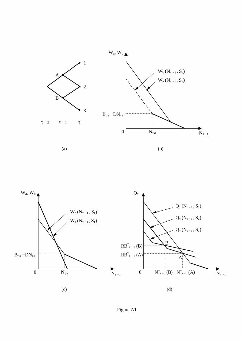
B •
•A
•
•
• 1
2
3
τ − 2 τ − 1 τ
(a)
Figure A1
0
Bτ a −DNτ a
Nτ a Nτ − 1
Wb (Nτ − 1 , Sτ)
Wa (Nτ − 1 , Sτ)
(b)
Wa, Wb
0
Bτ a −DNτ a
Nτ a Nτ − 1
Wb (Nτ − 1 , Sτ)
Wa (Nτ − 1 , Sτ)
(c)
Wa, Wb
A
B
Qτ (Nτ − 1 , S2)
RB*τ − 1 (A)
RB*τ − 1 (B)
N*τ − 1 (B)0 N*
τ − 1 (A) Nτ − 1
Qτ (Nτ − 1 , S1)
Qτ (Nτ − 1 , S3)
(d)
Qτ

Note: Values indicate the slopes of the constraints.
X
−u(1−k)S−Dk
−u(1−k)S
−u(1+k)S+Dk
−d(1−k)S
−d(1+k)S+Dk
−d(1−k)S−Dk
Ñ=Nτ − 1Nτ b(u) Nτ b(d) −10 Nτ − 1
Figure A2
RHS of (14a)

Figure A3
Nτ − 1
A
X −u(1−k)S−Dk
−u(1+k)S+Dk
−d(1+k)S+Dk
−d(1−k)S−Dk
ÑNτ b(u) Nτ b(d) −10 Nτ − 1
−d(1−k)S
−u(1−k)S
RHS of (14a)
Note: Values indicate the slopes of the constraints.
Top Related