


![Object-oriented Programming with PHP · Object-oriented Programming with PHP [2 ] Object-oriented programming Object-oriented programming is a popular programming paradigm where concepts](https://static.fdocuments.us/doc/165x107/5e1bb46bfe726d12f8517bf0/object-oriented-programming-with-php-object-oriented-programming-with-php-2-object-oriented.jpg)


Languages
Pages
Legal


Object identification techniques for object-oriented verification
Mike BaldwinCIMMS/University of Oklahoma

Baldwin’s presentation on object-oriented verification
Harold BrooksNSSL

Issues
• Object identification –how many objects do you see?
• How to characterize and measure differences between objects?
• Dealing with different numbers of observed and forecast objects

Automated rainfall object identification
• Contiguous regions of measurable rainfall (similar to Ebert and McBride 2000)

Connected component labeling
• Pure contiguous rainfall areas result in 34 unique “objects” in this example
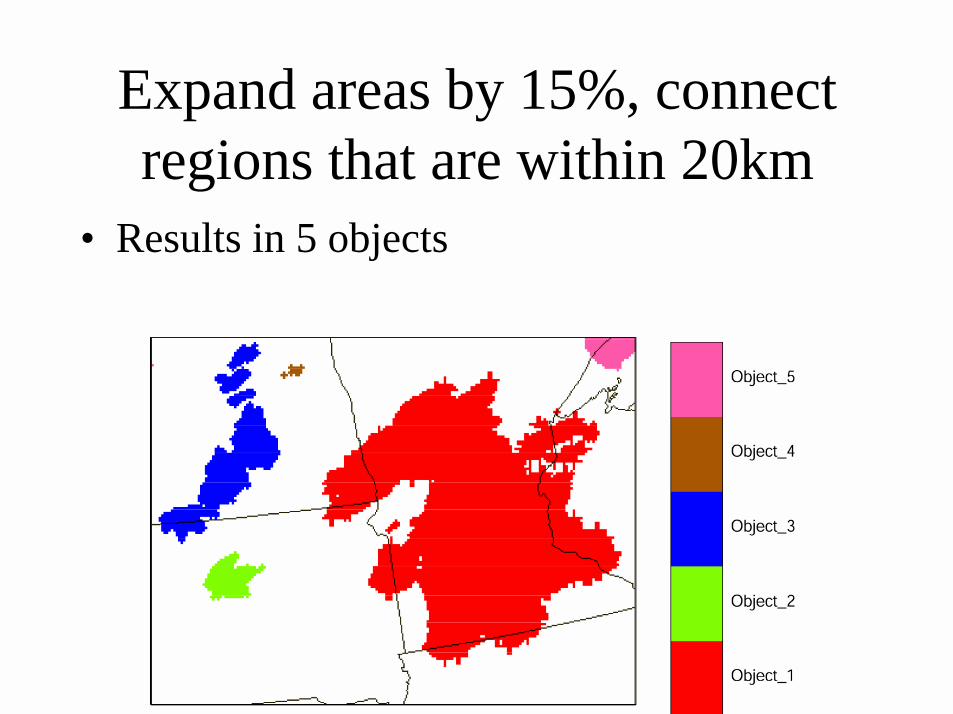
Expand areas by 15%, connect regions that are within 20km
• Results in 5 objects

Useful characterization
• Attributes related to rainfall intensity and auto-correlation ellipticity were able to produce groups of stratiform, cellular, linear rainfall systems in cluster analysis experiments
• However, autocorrelation calculation is SLOW

New auto-correlation attributes
• Replaced ellipticityof AC contours with max-min correlation at specific lags (50, 100, 150km, every 10°)
−0.2
−0.1
0
0.1
0.2
0.3
0.4
0.5
0.6
0.7
0.8
−60 −40 −20 0 20 40 60
−60
−40
−20
0
20
40
60

Attributes
• Area (km2), lat, lon• Mean, std dev (σ) of precip (mm) within object• Difference between max & min correlation at 50,
100, 150km lags (∆corr)• Orientation angle (θ) of max correlation at 50,
100, 150km lags (E-W = 0°, N-S=90°)• Each object is characterized by 11 attributes, with
a wide variety of units, ranges of values, etc.

How to measure “distance” between objects
• How to weigh different attributes?– Is 250km spatial distance same as 5mm precipitation
distance?
• Do attribute distributions matter?– Is 55mm-50mm same as 6mm-1mm?
• How to standardize attributes?– X'=(x-min)/(max-min)– X'=(x-mean)/σ– LEPS
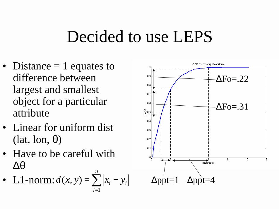
Decided to use LEPS• Distance = 1 equates to
difference between largest and smallest object for a particular attribute
• Linear for uniform dist (lat, lon, θ)
• Have to be careful with ∆θ
• L1-norm: ∆ppt=4∆ppt=1
∆Fo=.22
∆Fo=.31
∑=
−=n
iii yxyxd
1),(

NSSL/SPC Spring Program 2004
Observed ppt = Stage II (radar-only) 4km 1h accum• Comparison for ~1 month (May 10 – Jun 4)
Eta + ADAS + Level II
Eta (interp 40km grid)
Eta (interp 40 km)Init cond
YSU PBL, Lin et al. micro, Dudhia-RRTM rad
YSU PBL, Lin et al. micro,Dudhia-RRTM rad
MYJ PBL Ferrier micro, GFDL rad
Physics
4.0km/ 51 lvls4.0km/ 35 lvls4.5km/ 35 lvlsHorz/ vert grid
WRF-CAPSWRF-NCARWRF-NMM

Object ID and characterization
• Remapped each model to same grid as Stage II, common domain for all
• Run object ID, get attributes
• Create database of objects meso-α scale and larger [~ (200 km)2]

How to match observed and forecast objects?
F2 = false alarm
F1
O2
O3
O1 = missed event
dij = ‘distance’ between F iand O j

How to match observed and forecast objects?
F2 = false alarm
F1
O2
O3
O1 = missed event
Objects might “match” more than once…
If di* > dT then false alarm
If d*j > dT : missed event

Estimate of dT threshold
• Compute distance between each observed object and all others at the same time
• dT = 25th percentile = 2.5
• Forecasts have similar distributions
25th %-ile
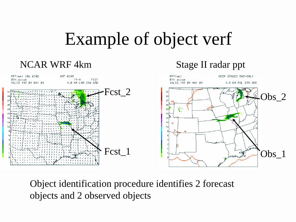
Example of object verf
Fcst_1
NCAR WRF 4km Stage II radar ppt
Obs_2Fcst_2
Obs_1
Object identification procedure identifies 2 forecast objects and 2 observed objects

Fcst_1
NCAR WRF 4km
Stage II radar ppt
Attributes
Area=70000 km2
mean(ppt)=0.97
σ (ppt)= 1.26
∆corr(50)=1.17
∆corr(100)=0.99
∆corr(150)=0.84
θ(50)=173°
θ(100)=173°
θ(150)=173°
lat = 40.2°N
lon = 92.5°W
Fcst_2 Obs_1 Obs_2
Area=70000 km2
mean(ppt)=0.60
σ (ppt)= 0.67
∆corr(50)=0.36
∆corr(100)=0.52
∆corr(150)=0.49
θ(50)=85°
θ(100)=75°
θ(150)=65°
lat = 44.9°N
lon =84.5°W
Area=135000
mean(ppt)=0.45
σ (ppt)= 0.57
∆corr(50)=0.37
∆corr(100)=0.54
∆corr(150)=0.58
θ(50)=171°
θ(100)=11°
θ(150)=11°
lat = 39.9°N
lon = 91.2°W
Area=285000
mean(ppt)=0.32
σ (ppt)= 0.44
∆corr(50)=0.27
∆corr(100)=0.42
∆corr(150)=0.48
θ(50)=95°
θ(100)=85°
θ(150)=85°
lat = 47.3°N
lon = 84.7°W
Obs_2
Obs_1

Distances between objects
• After transforming raw attributes to probability space (observed CDF: LEPS)
• Using L1-norm (Manhattan distance)
Fcst_1, Obs_1 : 1.48 [match]
Fcst_2, Obs_1 : 2.74
Fcst_1, Obs_2 : 2.75
Fcst_2, Obs_2 : 1.39 [match]
Obs_1, Obs_2 : 2.18
Fcst_1, Fcst_2 : 3.81

Average distances for matching fcst and obs objects
• 1-30h fcsts, 10 May – 03 June 2004• Eta (12km) = 2.12• WRF-CAPS = 1.97• WRF-NCAR = 1.98• WRF-NMM = 2.02

With set of matching obs and fcsts
• Nachamkin (2004) compositing ideas– errors given fcst event– errors given obs event
• Distributions of errors for specific attributes• Use classification to stratify errors by
convective mode
Top Related