


Languages
Pages
Legal

DES-TIME-2006
Dresden International Symposium on Technology and its Integration into Mathematics Education 2006
9th ACDCA Summer Academy
7th Int’l Derive & TI-CAS Conference
20-23 July 2006, Dresden, Germany
Numerical methods with the Voyage 200: to function or to program, That is the question!
Gilles PICARD and Chantal TROTTIER Ecole de technologie supérieure
1100, Notre-Dame street West, Montreal (Quebec) Canada [email protected]
ABSTRACT We teach a variety of math topics (Calculus of one and several variables, Differential Equations…) in a Technical Engineering School. The Voyage 200 is mandatory for all new full-time students. We encounter in these courses a few classical numerical methods (Newton’s method, numerical integration, Euler or Runge-Kutta methods). Beside the theoretical aspects, these methods are usually illustrated using functions or programs already defined in a CAS or using files or worksheets where students only have to modify some parameters and observe the results. Having to teach a course where numerical methods would be the main subject for about 4 weeks, we decided to ask students to program some of these algorithms using their TI symbolic calculators. We will explain briefly the differences between a function and a program on these calculators and show examples of the functions used normally in classrooms for the illustration of the classical methods. We will then see how to incorporate important aspects (number of iterations, tolerance, etc.) in the programming of these functions. Why should we want to create a program instead of a function? We will illustrate this with more complex algorithms, using examples from linear algebra (Cholesky and Gauss-Seidel methods) and even show examples of programs done by students. The aim here was to give students the interest and the ability to create their own programs on their calculator, showing them the advantage of programming in an environment where a great number of math-functions already exist. We were also able to create exam questions based on these programs and methods; examples will be shown in our presentation. We have observed more interest from the students for this topic when we asked them to program their calculators with these algorithms. Many of them were surprised how easy it was. Perhaps, teachers could see with their students slightly more complex functions or programs illustrating these numerical methods.
2
1. Introduction
Teaching basic mathematics in an engineering curriculum, we are used to see some classic
numerical methods, for example solutions of equations with Newton’s method, numerical
integration with Simpson’s method, solutions of differential equations with Euler’s or Runge-
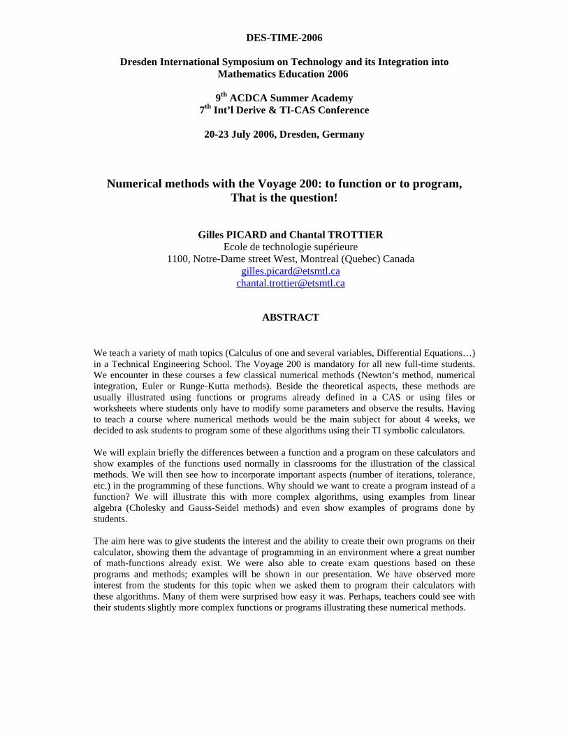
Kutta’s method. Students learn early on how to put a function in memory of their Voyage 200
calculators (everyone has it on his desktop in the classrooms). This is one of the first thing they
learn with the use of the symbolic calculator. We insist that the calculator does not merely put the
algebraic expression in memory but it’s more like a small program which, for the example below,
will associate cos( )t t− to the input t. Changing the input will not change what the function has to
do. Of course, if the variable used has an assigned value, this will reflect the output of the function.
Figure 1
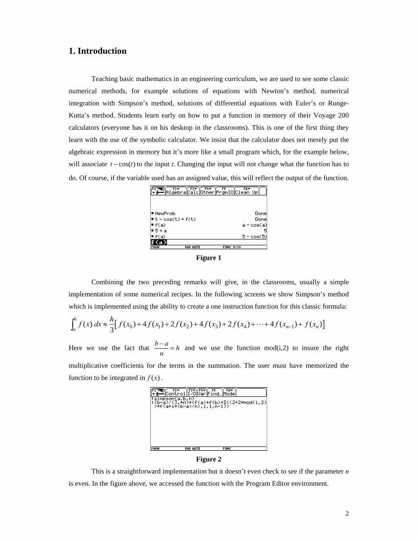
Combining the two preceding remarks will give, in the classrooms, usually a simple
implementation of some numerical recipes. In the following screens we show Simpson’s method
which is implemented using the ability to create a one instruction function for this classic formula:
[ ]0 1 2 3 4 1( ) ( ) 4 ( ) 2 ( ) 4 ( ) 2 ( ) 4 ( ) ( )3
bn na
hf x dx f x f x f x f x f x f x f x−≈ + + + + + + +∫
Here we use the fact that b a hn−
= and we use the function mod(i,2) to insure the right
multiplicative coefficients for the terms in the summation. The user must have memorized the
function to be integrated in ( )f x .
Figure 2
This is a straightforward implementation but it doesn’t even check to see if the parameter n
is even. In the figure above, we accessed the function with the Program Editor environment.
3
Another basic example is Newton’s method which is usually seen as an application of
derivatives for solving the equation ( ) 0f x = for a differentiable function. Let’s look at finding a
root of the equation cos( ) 0t t− = between 0 and 1. The classic iteration formula is
( )( )1
nn n
n
f xx x
f x+ = −′
starting with an appropriate initial value 0x . If we want to keep things simple
for the students, we’ll put the initial value in a variable (a for this example) and ask the Voyage
200 to evaluate ( )( )
f aa
f a−
′ and store the result again in variable a. Hitting the enter key calculates
the new value each time, a process that we can repeat until the value calculated doesn’t change
anymore, which happens here after 5 iterations (see figures 3a and 3b).
Figure 3a Figure 3b
We could also have defined a simple function named newton(a) which could do the same
thing.
Figure 4
This is fine in a first Calculus course but it would be better if we could have more control
on what happens, looking at the difference between two iterations or counting the number of
iterations needed for a specified precision.
2. Functions, from basics to more complex
Let’s look again at the Newton example and consider adding a verification in the function:
we want to verify if the tangent is horizontal and have a message announcing this when it happens
(of course Newton’s method fails in this case and will produce an undef answer). This will be

4
done be editing a copy of the function already in memory, using the Program Editor. The next two
screens show the initial function and the modified one where we added the verification.
Figure 5a Figure 5b
Having a function with more than one instruction, we have to use the delimiters
Func…EndFunc. The Voyage 200 uses classic and simple programming instructions, as showed in
figure 5b where the function newton1(a) starts to look more like a small program. Using this new
function still with the previous example of finding a root of cos( ) 0t t− = , but starting with
32
t π= , so that the derivative has zero value, we see that the function gives the right
warning.
Figure 6
It would be natural next to try to control the precision obtained from one iteration to the
next and to have a count of the number of iterations necessary to obtain a specified precision. We
would like to implement the following rule: stop the iterations when the difference (in absolute
value) of two consecutive iterations is less than a specified tolerance, let’s call this value tol. We
will add a maximum number of iterations (maxit) for convergence, to eliminate the possibility of a
divergent process we would have to stop manually. Of course we would like the function to return
two values: the result of the iterations and the number of steps needed to satisfy the tolerance
specified. This challenges one limitation of working with functions, the output in the Home
environment will be the result of the last line of code in the function. We will elude this problem
by creating a list containing two elements: the resulting solution and the number of steps needed.
Let’s look in the following screens how the previous function is modified to incorporate these
changes.

5
Figure 7a Figure 7b
We see that the function newton2 now has 3 parameters, a being the initial value to start
the iterations, tol the desired tolerance and maxit the maximum number of iterations. We have
defined two local variables m and xn, m is for counting the number of iterations and xn is the new
value obtained from the old one which is a (this is needed to evaluate the difference in absolute
value between two consecutive iterations). We use a loop command to iterate the process, ending it
when the tangent is horizontal or when the specified precision is obtained or when the maximum
number of iterations is reached. The last line of code executed will be a message of error or a list
containing the number of iterations (m), and the solution found (xn)
Let’s solve again the initial problem of finding a root of the equation cos( ) 0t t− =
between 0 and 1. We’ll use a maximum number of iterations of 10 and a tolerance of
0.00005. We see in the following screen that if we start the process with 1a = , we find in
3 steps a solution satisfying the desired tolerance.
Figure 8
If we start with 5a = , the calculator gives, after 10 steps, a false solution. Of
course, when using Newton’s method one must remember to use a starting point near the
desired solution to insure convergence. When our function returns a number of steps equal
to the maximum number of steps, one has to be suspicious of the result given. Finally, if
the function encounters a null value for the derivative, we’ll get an error message.
6
Looking at this last version of our Newton function, this really seems to be more a
program than a function, using classic code for creating loops, using conditional testing…
The user of this function still has to put the correct function to solve in a global memory,
( )f x in our example, and he has to decide a good starting value for the iterations to
converge. An advantage of functions like this one is that the result is given in the Home
environment and can be used in other calculations. Using the Voyage 200 for
programming is quite interesting since one can use in their own functions or programs,
system functions already implemented. We use in our function a command for the
calculation and evaluation of the derivative of a function at a given value. So the big
question, what is the difference between a function and a program, why use one instead of
the other?
3. From functions to programs
A function can be called in the Home environment and will return only one value or
expression there. It cannot create or modify a global variable in memory, but can use a value
already assigned in a global memory variable. A program on the other hand can create or modify
global variables as well as work with local variables. The only initial difference in the code is the
first and last line of code where Prgm and EndPrgm will replace the function delimiters Func and
EndFunc. A program will not return a value in the Home environment but has more elaborate
options for Input/Output using the “PrgmIO” screen accessed with F5 in the Home environment.
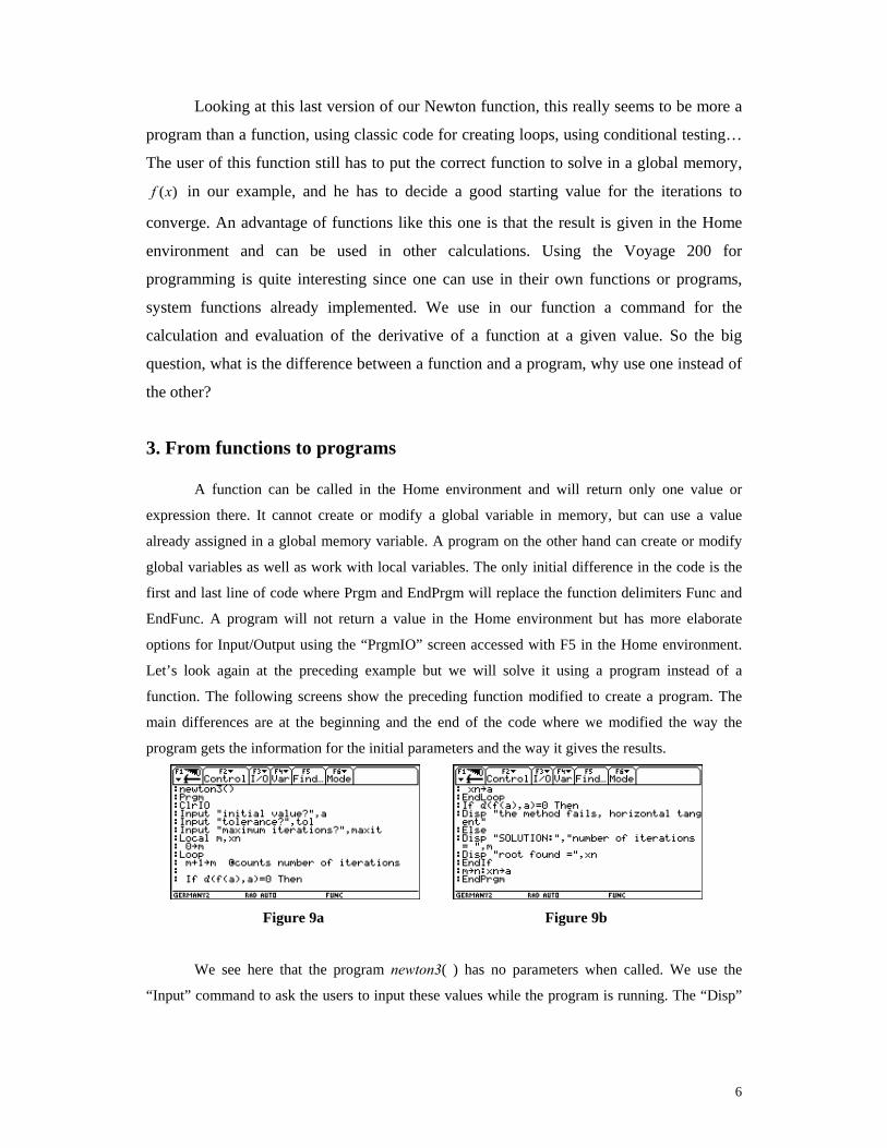
Let’s look again at the preceding example but we will solve it using a program instead of a
function. The following screens show the preceding function modified to create a program. The
main differences are at the beginning and the end of the code where we modified the way the
program gets the information for the initial parameters and the way it gives the results.
Figure 9a Figure 9b
We see here that the program newton3( ) has no parameters when called. We use the
“Input” command to ask the users to input these values while the program is running. The “Disp”
7
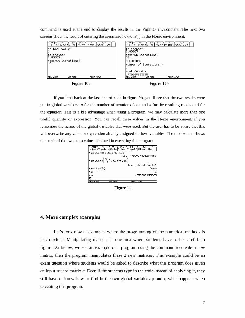
command is used at the end to display the results in the PrgmIO environment. The next two
screens show the result of entering the command newton3( ) in the Home environment.
Figure 10a Figure 10b
If you look back at the last line of code in figure 9b, you’ll see that the two results were
put in global variables: n for the number of iterations done and a for the resulting root found for
the equation. This is a big advantage when using a program; we may calculate more than one
useful quantity or expression. You can recall these values in the Home environment, if you
remember the names of the global variables that were used. But the user has to be aware that this
will overwrite any value or expression already assigned to these variables. The next screen shows
the recall of the two main values obtained in executing this program.
Figure 11
4. More complex examples
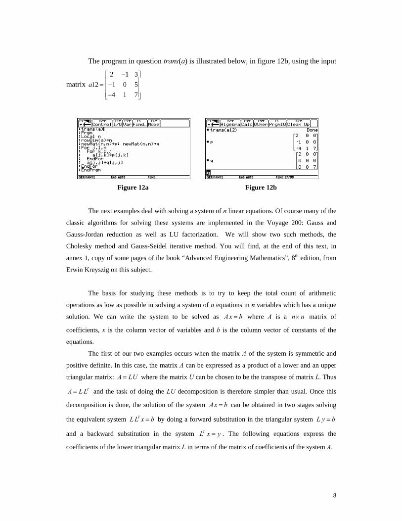
Let’s look now at examples where the programming of the numerical methods is
less obvious. Manipulating matrices is one area where students have to be careful. In
figure 12a below, we see an example of a program using the command to create a new
matrix; then the program manipulates these 2 new matrices. This example could be an
exam question where students would be asked to describe what this program does given
an input square matrix a. Even if the students type in the code instead of analyzing it, they
still have to know how to find in the two global variables p and q what happens when
executing this program.
8
The program in question trans(a) is illustrated below, in figure 12b, using the input
matrix 2 1 3
12 1 0 54 1 7
a−⎡ ⎤
⎢ ⎥= −⎢ ⎥⎢ ⎥−⎣ ⎦
Figure 12a Figure 12b
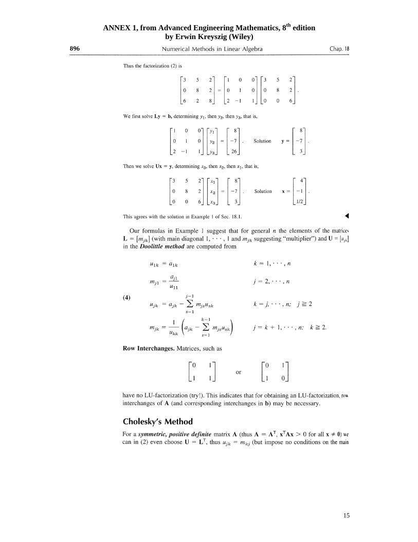
The next examples deal with solving a system of n linear equations. Of course many of the
classic algorithms for solving these systems are implemented in the Voyage 200: Gauss and
Gauss-Jordan reduction as well as LU factorization. We will show two such methods, the
Cholesky method and Gauss-Seidel iterative method. You will find, at the end of this text, in
annex 1, copy of some pages of the book “Advanced Engineering Mathematics”, 8th edition, from
Erwin Kreyszig on this subject.
The basis for studying these methods is to try to keep the total count of arithmetic
operations as low as possible in solving a system of n equations in n variables which has a unique
solution. We can write the system to be solved as A x b= where A is a n n× matrix of
coefficients, x is the column vector of variables and b is the column vector of constants of the
equations.
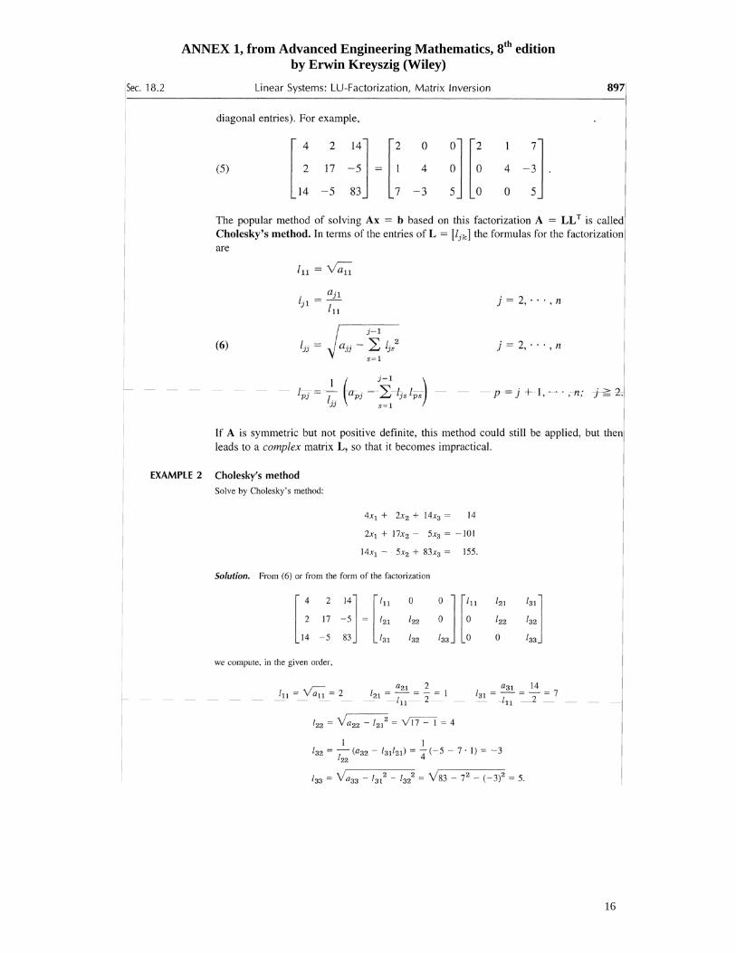
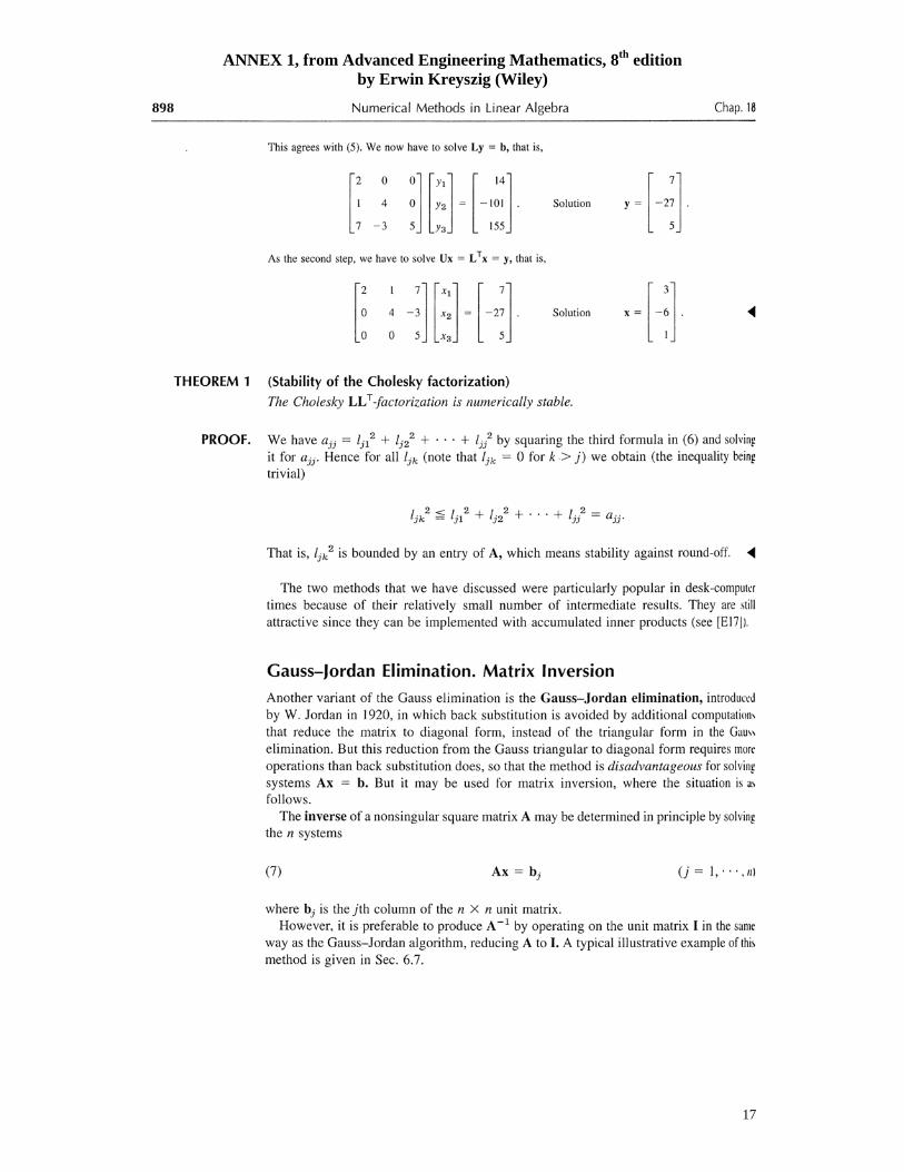
The first of our two examples occurs when the matrix A of the system is symmetric and
positive definite. In this case, the matrix A can be expressed as a product of a lower and an upper
triangular matrix: A LU= where the matrix U can be chosen to be the transpose of matrix L. Thus
TA L L= and the task of doing the LU decomposition is therefore simpler than usual. Once this
decomposition is done, the solution of the system A x b= can be obtained in two stages solving
the equivalent system TL L x b= by doing a forward substitution in the triangular system L y b=
and a backward substitution in the system TL x y= . The following equations express the
coefficients of the lower triangular matrix L in terms of the matrix of coefficients of the system A.

9
11 11
11
11
12
1
1
1
2, ,
2, ,
1 1, , ; 2
jj
j
jj jj jss
j
pj pj js pssjj
l aa
l j nl
l a l j n
l a l l p j n jl
−
=
−
=
=
= =
= − =
⎛ ⎞= − = + ≥⎜ ⎟
⎝ ⎠
∑
∑
The following screens show a function, implementing these equations, on the Voyage 200
which will be used to calculate the lower triangular matrix L of a symmetric matrix A. In some
semester, this function was given to student to illustrate programming and manipulating matrices
with the Voyage 200, in other semester, students were asked to program this decomposition and
gives us back their code with documentation which was then graded. You may notice the code
used below which is almost identical to the given formulas.
Figure 13a Figure 13b
Here is a numeric example with the matrix 4 2 142 17 5 13
14 5 83a
⎡ ⎤⎢ ⎥− =⎢ ⎥⎢ ⎥−⎣ ⎦
(see annex 1 for more
details with this example):
Figure 14
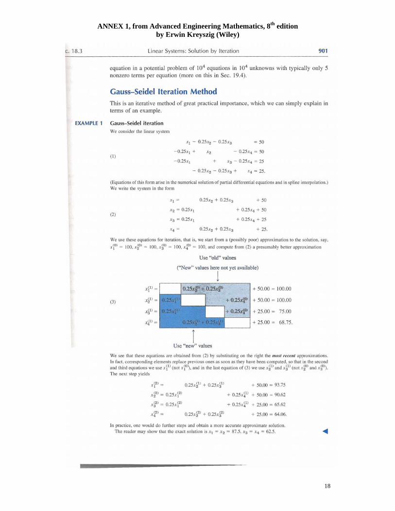
The last example is Gauss-Seidel method for solving the same linear system A x b= , but
using an iterative approach using an initial guess solution (0)x and calculating a sequence (1) (2) ( ), , , nx x x where each column vector ( )ix should be closer and closer to the solution of the
system. We stop this process when we obtain a specified accuracy. This is kind of a vector-based
10
fixed point iteration process and it requires some conditions to be convergent and to provide a
faster algorithm than the other classic methods. It can be interesting in large sparse system, with
many 0 entries, with large diagonal values with respect to the other entries in each line of the
matrix A. If we look at the example in annex 1, we see in fact the similarities with the fixed point
method where we iterate this equation: 1 ( )n nx f x+ = . In some semester, we asked students to
implement this method on their Voyage 200. This is the algorithm from Kreyszig’s book (page
902):
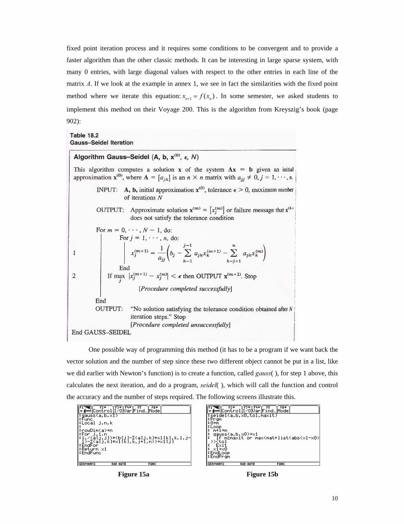
One possible way of programming this method (it has to be a program if we want back the
vector solution and the number of step since these two different object cannot be put in a list, like
we did earlier with Newton’s function) is to create a function, called gauss( ), for step 1 above, this
calculates the next iteration, and do a program, seidel( ), which will call the function and control
the accuracy and the number of steps required. The following screens illustrate this.
Figure 15a Figure 15b
11
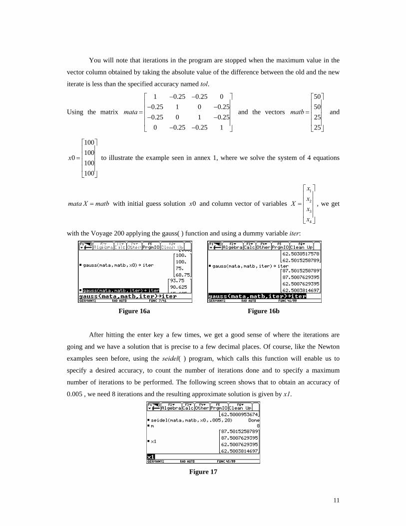
You will note that iterations in the program are stopped when the maximum value in the
vector column obtained by taking the absolute value of the difference between the old and the new
iterate is less than the specified accuracy named tol.
Using the matrix
1 0.25 0.25 00.25 1 0 0.250.25 0 1 0.250 0.25 0.25 1
mata
− −⎡ ⎤⎢ ⎥− −⎢ ⎥=⎢ ⎥− −⎢ ⎥− −⎣ ⎦
and the vectors
50502525
matb
⎡ ⎤⎢ ⎥⎢ ⎥=⎢ ⎥⎢ ⎥⎣ ⎦
and
100100
0100100
x
⎡ ⎤⎢ ⎥⎢ ⎥=⎢ ⎥⎢ ⎥⎣ ⎦
to illustrate the example seen in annex 1, where we solve the system of 4 equations
mata X matb= with initial guess solution 0x and column vector of variables
1
2
3
4
xx
Xxx
⎡ ⎤⎢ ⎥⎢ ⎥=⎢ ⎥⎢ ⎥⎣ ⎦
, we get
with the Voyage 200 applying the gauss( ) function and using a dummy variable iter:
Figure 16a Figure 16b
After hitting the enter key a few times, we get a good sense of where the iterations are
going and we have a solution that is precise to a few decimal places. Of course, like the Newton
examples seen before, using the seidel( ) program, which calls this function will enable us to
specify a desired accuracy, to count the number of iterations done and to specify a maximum
number of iterations to be performed. The following screen shows that to obtain an accuracy of
0.005 , we need 8 iterations and the resulting approximate solution is given by x1.
Figure 17
12
5. Examples from students
The next examples will show briefly work done by students where the assignment was to
program and document either Gauss-Seidel’s or Cholesky’s method on their symbolic calculators.
They had to give us the programs so we could test them.
Example 1:
This is a simple program which does Gauss-Seidel iterations. Here is the code:
seidelt(a,b,x0,err,maxloop) Prgm Local n,j rowDim(a)->n newMat(n,1)->xn For c,1,maxloop For j,1,n 1/(a[j,j]) * (b[j] - ∑(a[j,k]*xn[k],k,1,j-1) - ∑(a[j,k]*x0[k],k,j+1,n)) -> xn[j] EndFor If max(abs(xn-x0))[1,1] < err Then Exit Else xn->x0 EndIf EndFor EndPrgm
This is quite similar to what we showed in figure 15, but simpler, everything is done inside
the program; the number of iterations is in variable c and the solution is in the variable xn.
Example 2:
This next example, also with Gauss-Seidel, shows a function that could (may be) return
the right solution but there is no way of knowing the number of iterations done. Furthermore, there
is a problem if you don’t give the right value for the parameter n which is the number of equations
in the system (this should be done directly in the program with the appropriate command).
Figure 18a Figure 18b
13
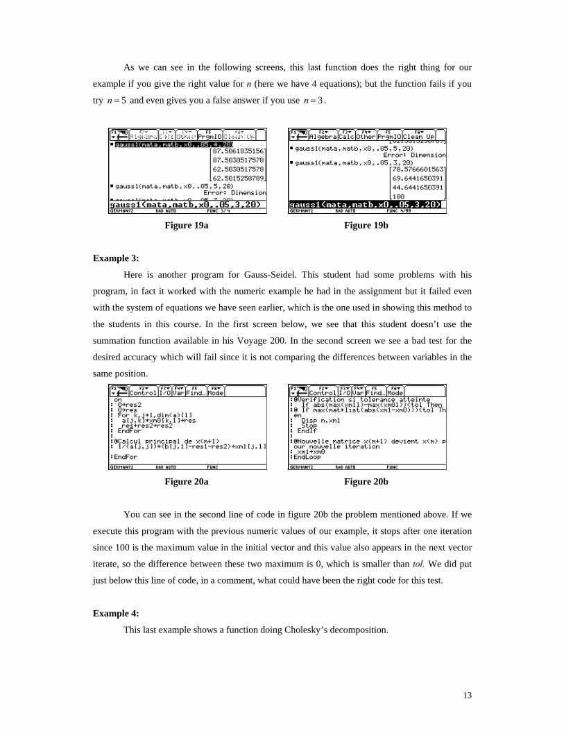
As we can see in the following screens, this last function does the right thing for our
example if you give the right value for n (here we have 4 equations); but the function fails if you
try 5n = and even gives you a false answer if you use 3n = .
Figure 19a Figure 19b
Example 3:
Here is another program for Gauss-Seidel. This student had some problems with his
program, in fact it worked with the numeric example he had in the assignment but it failed even
with the system of equations we have seen earlier, which is the one used in showing this method to
the students in this course. In the first screen below, we see that this student doesn’t use the
summation function available in his Voyage 200. In the second screen we see a bad test for the
desired accuracy which will fail since it is not comparing the differences between variables in the
same position.
Figure 20a Figure 20b
You can see in the second line of code in figure 20b the problem mentioned above. If we
execute this program with the previous numeric values of our example, it stops after one iteration
since 100 is the maximum value in the initial vector and this value also appears in the next vector
iterate, so the difference between these two maximum is 0, which is smaller than tol. We did put
just below this line of code, in a comment, what could have been the right code for this test.
Example 4:
This last example shows a function doing Cholesky’s decomposition.
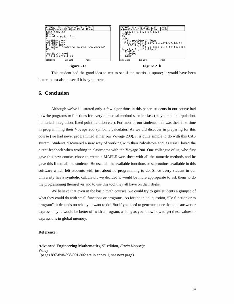
14
Figure 21a Figure 21b
This student had the good idea to test to see if the matrix is square; it would have been
better to test also to see if it is symmetric.
6. Conclusion
Although we’ve illustrated only a few algorithms in this paper, students in our course had
to write programs or functions for every numerical method seen in class (polynomial interpolation,
numerical integration, fixed point iteration etc.). For most of our students, this was their first time
in programming their Voyage 200 symbolic calculator. As we did discover in preparing for this
course (we had never programmed either our Voyage 200), it is quite simple to do with this CAS
system. Students discovered a new way of working with their calculators and, as usual, loved the
direct feedback when working in classrooms with the Voyage 200. One colleague of us, who first
gave this new course, chose to create a MAPLE worksheet with all the numeric methods and he
gave this file to all the students. He used all the available functions or subroutines available in this
software which left students with just about no programming to do. Since every student in our
university has a symbolic calculator, we decided it would be more appropriate to ask them to do
the programming themselves and to use this tool they all have on their desks.
We believe that even in the basic math courses, we could try to give students a glimpse of
what they could do with small functions or programs. As for the initial question, “To function or to
program”, it depends on what you want to do! But if you need to generate more than one answer or
expression you would be better off with a program, as long as you know how to get these values or
expressions in global memory.
Reference:
Advanced Engineering Mathematics, 9th edition, Erwin Kreyszig Wiley (pages 897-898-898-901-902 are in annex 1, see next page)
ANNEX 1, from Advanced Engineering Mathematics, 8th edition by Erwin Kreyszig (Wiley)
15
ANNEX 1, from Advanced Engineering Mathematics, 8th edition by Erwin Kreyszig (Wiley)
16
ANNEX 1, from Advanced Engineering Mathematics, 8th edition by Erwin Kreyszig (Wiley)
17
ANNEX 1, from Advanced Engineering Mathematics, 8th edition by Erwin Kreyszig (Wiley)
18

ANNEX 1, from Advanced Engineering Mathematics, 8th edition by Erwin Kreyszig (Wiley)
19
Top Related