


Languages
Pages
Legal


1
Numerical Methods
Process Systems Engineering
OPTIMIZATION
Numerical methods in chemical
engineering
Edwin Zondervan

2
Numerical Methods
Process Systems Engineering
OVERVIEW
• In this lecture we get introduced to constrained and unconstrained optimization.
• We will use the simplex method to solve linear programming problems (LP)
• We will use the Lagrange multiplier method to solve nonlinear programming problems (NLP’s)
• And we will briefly discuss optimal control, using Pontryagin’s principle.
• Lastly we will play a little with another optimization platform (AMPL)
3
Numerical Methods
Process Systems Engineering
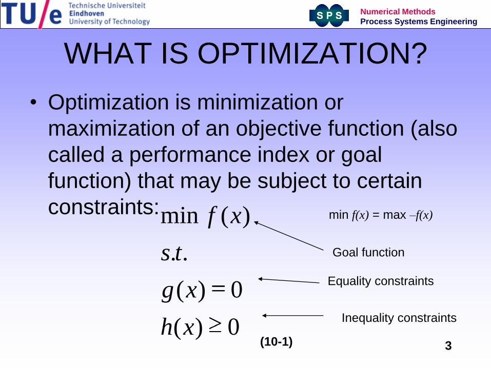
WHAT IS OPTIMIZATION?
• Optimization is minimization or
maximization of an objective function (also
called a performance index or goal
function) that may be subject to certain
constraints:
0)(
0)(
..
)(min
xh
xg
ts
xf
Goal function
Equality constraints
Inequality constraints
min f(x) = max –f(x)
(10-1)

4
Numerical Methods
Process Systems Engineering
OPTIMIZATION SPECTRUM
Problem Method Solvers
LP Simplex method
Barrier methods
Linprog (Matlab)
CPLEX (GAMS, AIMMS, AMPL,
OPB)
NLP
QP
Lagrange multiplier method
Successive linear programming
Quadratic programming
Fminsearch/fmincon (Matlab)
MINOS (GAMS, AMPL)
CONOPT (GAMS)
MIP
MILP
MINLP
MIQP
Branch and bound
Dynamic programming
Generalized Benders Decomposition
Outer Approximation method
Disjunctive programming
Bintprog (Matlab)
DICOPT (GAMS)
BARON (GAMS)
MATHEMATICAL PROGRAMMING
META HEURISTICS
Neural networks, fuzzy modeling, genetic algorithms,
expert systems, etc.
Constraint programming, stochastic programming, multi-
objective programming, etc.
ADVANCED TOPICS

5
Numerical Methods
Process Systems Engineering
FACTORS OF CONCERN
• Continuity of the functions
• Convexity of the functions
• Global versus local optima
• Constrained versus unconstrained optima

6
Numerical Methods
Process Systems Engineering
LINEAR PROGRAMMING
• In linear programming the objective
function and the constraints are linear
functions!
• For example:
0
0
6025
6082
..
8840),(max
2
1
21
21
2121
x
x
xx
xx
ts
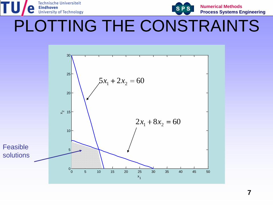
xxxxfz If the constraints are satisfied, but
the objective function is not
maximized/minimized we speak of
a feasible solution.
If also the objective function is
maximized/minimized, we speak of
an optimal solution!
(10-2)
7
Numerical Methods
Process Systems Engineering
PLOTTING THE CONSTRAINTS
0 5 10 15 20 25 30 35 40 45 500
5
10
15
20
25
30
x1
x2
6082 21 xx
6025 21 xx
Feasible
solutions

8
Numerical Methods
Process Systems Engineering
PLOTTING THE OBJECTIVE FUNCTION
0 5 10 15 20 25 30 35 40 45 500
5
10
15
20
25
30
x1
x2
z=0
z=840
Optimal
solution

9
Numerical Methods
Process Systems Engineering
NORMAL FORM OF AN LP PROBLEM
0
0
6025
6082
..
8040),(max
2
1
21
21
2121
x
x
xx
xx
ts
xxxxfz
}4,...,1{0
6025
6082
..
8840)(max
421
321
21
ix
xxx
xxx
ts
xxxf
i
x3 and x4 are called slack variables, they are
non auxiliary variables introduced for the
purpose of converting inequalities in to
equalities
NORMAL FORM OF THE LP PROBLEM
(10-3)

10
Numerical Methods
Process Systems Engineering
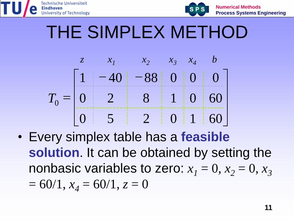
THE SIMPLEX METHOD
• We can formulate our earlier example to
the normal form and consider it as the
following augmented matrix:
6010250
6001820
00088401
0T
z x1 x2 x3 x4 b
This matrix is called the (initial) simplex tableEach simplex table has two kinds of
variables, the basic variables
(columns having only one nonzero
entry) and the nonbasic variables
(10-4)
11
Numerical Methods
Process Systems Engineering
THE SIMPLEX METHOD
• Every simplex table has a feasible
solution. It can be obtained by setting the
nonbasic variables to zero: x1 = 0, x2 = 0, x3
= 60/1, x4 = 60/1, z = 0
6010250
6001820
00088401
0T
z x1 x2 x3 x4 b

12
Numerical Methods
Process Systems Engineering
THE OPTIMAL SOLUTION?
• The optimal solution is now obtained
stepwise by pivoting in such way that z
reaches a maximum.
• The big question is, how to choose your
pivot equation …
13
Numerical Methods
Process Systems Engineering
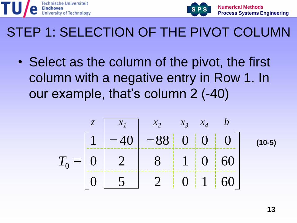
STEP 1: SELECTION OF THE PIVOT COLUMN
• Select as the column of the pivot, the first
column with a negative entry in Row 1. In
our example, that’s column 2 (-40)
6010250
6001820
00088401
0T
z x1 x2 x3 x4 b
(10-5)
14
Numerical Methods
Process Systems Engineering
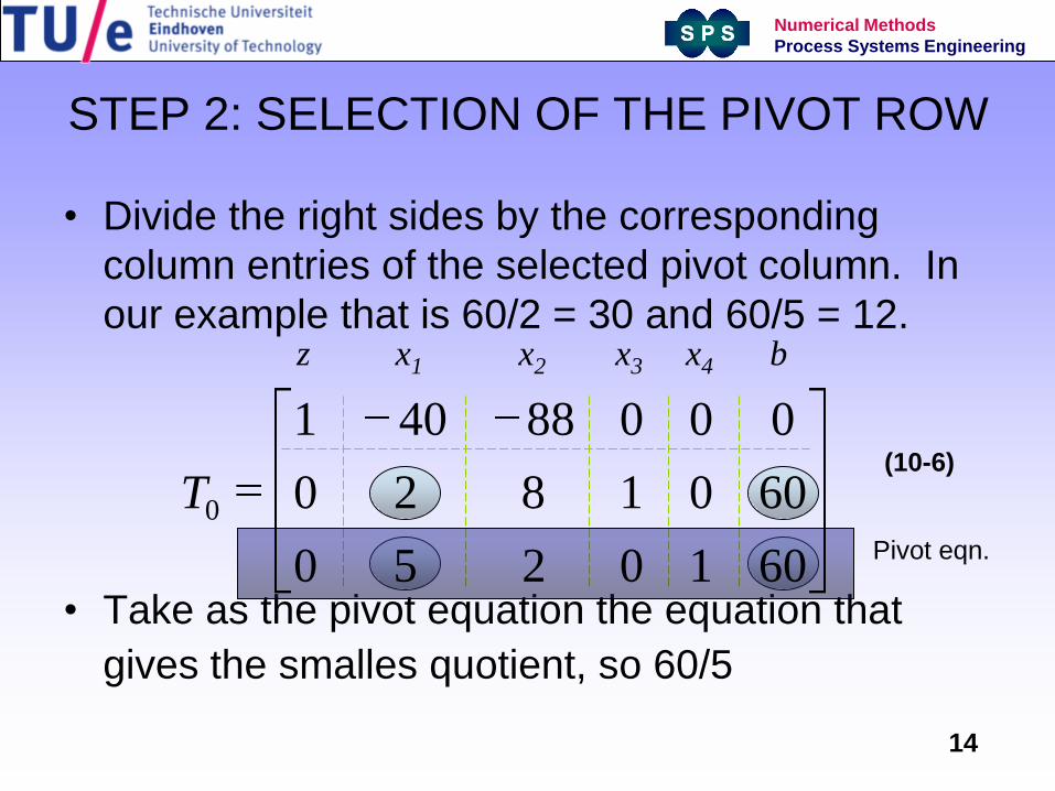
STEP 2: SELECTION OF THE PIVOT ROW
• Divide the right sides by the corresponding
column entries of the selected pivot column. In
our example that is 60/2 = 30 and 60/5 = 12.
• Take as the pivot equation the equation that
gives the smalles quotient, so 60/5
z x1 x2 x3 x4 b
Pivot eqn.
(10-6)
6010250
6001820
00088401
0T
15
Numerical Methods
Process Systems Engineering
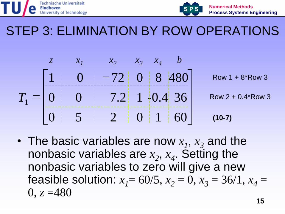
STEP 3: ELIMINATION BY ROW OPERATIONS
• The basic variables are now x1, x3 and the nonbasic variables are x2, x4. Setting the nonbasic variables to zero will give a new feasible solution: x1= 60/5, x2 = 0, x3 = 36/1, x4 = 0, z =480
6010250
36-0.417.200
480807201
1T
z x1 x2 x3 x4 b
Row 1 + 8*Row 3
Row 2 + 0.4*Row 3
(10-7)
16
Numerical Methods
Process Systems Engineering
THE SIMPLEX METHOD
• We moved from z = 0 to z = 480. The reason
for the increase is because we eliminated a
negative term from the eqation, so:
elimination should only be applied to negative
entries in Row 1, but no others.
• Although we found a feasible solution, we did
not find the optimal solution yet (the entry of -
72 in our simplex table) so we repeat step
1 to 3.

17
Numerical Methods
Process Systems Engineering
THE SECOND ITERATION
• Step 1: select column 3
• Step 2: 36/7.2 = 5 and 60/2 = 30 select 7.2 as the pivot
• Elimination by row operations:
• The basic feasible solution: x1= 50/5, x2 = 36/7.2, x3 = 0, x4 = 0, z =840 (no more negative entries: so this solution is also the optimal solution)
509.0/136/1050
364.012.700
840410001
2T
Row 1 + 10*Row 2
Row 3 – (2/7.2)*Row 2
(10-8)

18
Numerical Methods
Process Systems Engineering
USING MATLAB FOR LP PROBLEMS
• We are going to solve
the following LP
problem:
Using the function
LINPROG:f = [-5; -4; -6]
A = [1 -1 1 3 2 4 3 2 0];
b = [20; 42; 30];
lb = zeros(3,1);
[x,fval,exitflag,output,lambda]
= linprog(f,A,b,[],[],lb);
Gives:x = 0.00 15.00 3.00
lambda.ineqlin = 0 1.50 0.50
lambda.lower = 1.00 0 0
321
21
321
321
321
x, 0 x, 0 x0
302x3x
424x2x3x
20x– xx
ts
–6x– 4x–5xxf
..
)(min
(10-9)

19
Numerical Methods
Process Systems Engineering
NONLINEAR PROGRAMMING
• In nonlinear programming the objective
function and the constraints are nonlinear
functions!
• For example:
52)(
..
35)(min
21
2
2
2
1
xxxg
ts
xxxf
(10-10)
20
Numerical Methods
Process Systems Engineering
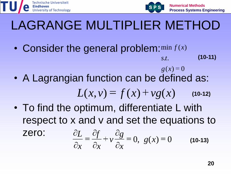
LAGRANGE MULTIPLIER METHOD
• Consider the general problem:
• A Lagrangian function can be defined as:
• To find the optimum, differentiate L with
respect to x and v and set the equations to
zero:
0)(
..
)(min
xg
ts
xf
)()(),( xvgxfvxL
0)(,0 xgx
gv
x
f
x
L
(10-11)
(10-12)
(10-13)

21
Numerical Methods
Process Systems Engineering
BACK TO THE EXAMPLE
52)(
..
35)(min
21
2
2
2
1
xxxg
ts
xxxf
17/25,17/30,17/150
052)(
06
0210
)52(35
21
21
2
2
1
1
21
2
2
2
1
xxv
xxxgv
L
vxx
L
vxx
L
xxvxxL
(10-14)
(10-15)

22
Numerical Methods
Process Systems Engineering
LMM FOR NLPs WITH INEQUALITY
CONSTRAINTS• When the problem has the following
shape:
• The Lagrangian function is defined as:
},...,1{0)(
},...,1{0)(
..
)(min
pmixg
mjxh
ts
xf
i
j
m
j
p
mj
jjjj xguxhvxfvuxL1 1
)()()(),,(
0)()()(11
xguxhvxf j
p
mj
jj
m
j
jThis condition, known as the Karush-
Kuhn-Tucker condition for optimality
should be satisfied.
(10-16)
(10-17)
(10-18)

23
Numerical Methods
Process Systems Engineering
USING MATLAB FOR NLP
PROBLEMS• We are going to solve
the following NLP problem:
Using the function FMINCON:
function f = myfun(x) f = -
x(1) * x(2) * x(3);
A=[-1 -2 -2; 1 2 2]; b = [0
72];
x0 = [10; 10; 10];
solution [x,fval] =
fmincon(@myfun,x0,A,b)
Gives:x = 24.00 12.00 12.00
722x2xx0
ts
xx–xf(x)
321
321
..
min
(10-19)
24
Numerical Methods
Process Systems Engineering
SOME TIPS FOR SOLVING NLPPs
• Avoid nonlinearity if possible
• Better nonlinearities in the objective
function than in the constraints
• Better inequalities than equalities
• Supply good starting guesses to a solver
• Don’t blame the solver if you don’t find a
solution, take a critical look at the problem
formulation
Top Related