


![NASA Contractor Report 195070 ICASE Report No. 95-27 … NASA Contractor Report 195070 ICASE Report No. 95-27 ... 5.1 The Zonal Fine Grid Scheme 50 ... 15, 16, 17]. Thus, the essential](https://static.fdocuments.us/doc/165x107/5abcbd497f8b9a76038e424d/nasa-contractor-report-195070-icase-report-no-95-27-contractor-report-195070.jpg)


Languages
Pages
Legal


o NASA Contractor Report 189611 NASA-CR-189611ICASE Report No. 92-6 19920011272
ICASECOMPRESSIBLE HOMOGENEOUS SHEAR:SIMULATION AND MODELING
S. SarkarG. ErlebacherM. Y. Hussaini
Contract No. NAS1-18605
February 1992
Institute for Computer Applications in Science and EngineeringNASA Langley Research CenterHampton, Virginia 23665-5225
Operated by the Universities Space Research Association
N/_A LIBRARY....CO__PYNationalAeronautics and A_ 99Space Administration I ! 2,
Langley Research CenterHampton,Virginia23665-5225 LANGLEYRESEARCHCENTER:_il
•LIBRARYNASA .::!i:HAMPTO_VIRGINIA
https://ntrs.nasa.gov/search.jsp?R=19920011272 2018-05-06T16:57:08+00:00Z


89433
Compressible Homogeneous Shear:Simulation and Modeling*
S. Sarkar, G. Erlebacher, and M.Y. Hussaini
Institute for Computer Applications in Science and Engineering
NASA Langley Research Center
Hampton, VA 23665
ABSTRACT
The present study investigates compressibility effects on turbulence by direct numerical
simulation of homogeneous shear flow. A primary observation is that the growth of the
turbulent kinetic energy decreases with increasing turbulent Mach number. The sinks pro-
vided by compressible dissipation and the pressure-dilatation, along with reduced Reynolds
shear stress, are shown to contribute to the reduced growth of kinetic energy. Models are
proposed for these dilatational terms and verified by direct comparison with the simulations.
The differences between the incompressible and compressible fields are brought out by the
examination of spectra, statistical moments, and structure of the rate of strain tensor.
*Researchwas supported by the National Aeronautics and Space Administration under NASA ContractNo. NAS1-18605while the authors werein residence at the Institute for Computer Applications in Scienceand Engineering(ICASE), NASA LangleyResearch Center, Hampton, VA23665.
i

1 Introduction
Homogeneous turbulent flow has long been viewed as a simple model of turbulence which
is sufficiently realistic to have fundamental physical features that persist in more complex
flows. For example, hairpin vortices which have been observed in boundary layer experiments
and simulations of channel flow, have been identified through direct numerical simulation
(DNS) of homogeneous shear flow by Rogers and Moin (1987). Similarly, the longitudinal
streaks observed in wall boundary layers have been shown by the simulations of Lee, Kim
and Moin (1990) to exist in homogeneous shear flow when the shear rate is high enough
to be comparable to those encountered near the wall in boundary layers. Rogallo (1981),who was the first to perform DNS of this flow, showed by direct comparison with physical
experiments that the simulated flow statistics were in good agreement with experimental
data.
In the past several years, there has been a strong activity in the area of compressible
turbulent simulations. The first fundamental study of compressible isotropic turbulence
was conducted by Passot and Pouquet (1987) who demonstrated the presence of shocks
in the flow. Their results motivated the study by Erlebacher et al. (1990) to classify the
different possible regimes in isotropic turbulence attainable from arbitrary initial conditions.
They quantified the conditions for the presence or absence of shocks. Other results on
decaying isotropic turbulence can be found in Sarkar et al. (1989), Lee, Lele and Moin
(1990), and Zang, Dahlburg, and Dahlburg (1992). Results on forced isotropic turbulence
are also available (Kida and Orszag 1990). Simulations have now moved on to the next
level of complexity, namely, homogeneous turbulence subjected to a linear mean velocity
field. For example, Coleman and Mansour (1991) have considered turbulence subjected to
homogeneous compression.
Homogeneous shear turbulence has a production term which continuously feeds energy
into the system, which then cascades down to the smaller scales. This flow exhibits some of
the properties of incompressible turbulent shear flows, with the added presence of acoustic
waves, density fluctuations, and dilatational velocity fields. Direct numerical simulations of
such flows can provide complete statistics not available from physical experiments. Com-
pressibility effects on the flow can be obtained from the simulations, and perhaps more
importantly, mechanisms responsible for these effects can be identified, and turbulence mod-
els for compressibility-related phenomena can be devised. The compressible problem was
considered by Feiereisen et al. (1982) who performed relatively low resolution 64a simula-
tions and concluded that compressibility effects are small. Recently Blaisdell, Mansour and
Reynolds (1990) have also considered compressible shear flow, and identified eddy shocklets
in the flow for high enough turbulence Reynolds and Mach number.
Research on the small-scale properties of homogeneous turbulence is primarily focussed
on understanding the intermittency of high dissipation regions. It has been numerically
established that the rate of strain tensor has a preferred shape in regions of strong dissipation
(Ashurst et al. 1987b). Furthermore, the vorticity tends to align with the intermediate
eigenvalue (whose most probable sign is positive). While this alignment property of the
vorticity is a consequence of a simplification of the Euler equations (Vieillefosse 1984), the
shape of the tensor is still unexplained. Alignment of other vectors have been considered by
Ashurst et al. (1987a).
In this paper, we use databases from the DNS of homogeneous compressible turbulence to
clarify the sources of reduced growth of kinetic energy with increased levels of compressibility.
This is then used to propose a new decomposition of pressure into incompressible and com-
pressible components. In turn, this leads to an improved model for the pressure-dilatation
term. Finally, we analyze the rate of strain tensor after decomposition into solenoidal and
irrotational components. Differences between the two tensors are brought out through the
use of one-dimensional probability functions.
2 Governing Equations
The compressible Navier-Stokes equations are written in a frame of reference moving with
the mean flow _1. This transformation, which was introduced by Rogallo (1981) for in-
compressible homogeneous shear, removes the explicit dependence on _1(x2) in the exact
equations for the fluctuating velocity, thus allowing periodic boundary conditions in the x2
* and the lab frame x_ isdirection. The relation between the moving frame xl
X 1 -- Xl -- S]_X 2 , X2 "-- 372 _ X3 _-- X 3
Here S denotes the constant shear rate fil,2. In the transformed frame x*, the compressible
Navier-Stokes equations take the form
asp+ - =0 (1)
I I _--- TI .Ot(puJ)+ (puju_),j -p,_+ ,_,_- Spu2%_
+ St(pu2'ui'),_ + Stp,_6i2 - Str'i_,_ (2)
Otp -t-uj'p,j . _/pu}j = Stu2'p,1 Jr 7Stpu_, 1 -t-
+ 2StT,,+StT I] (a)
2
p = pRT (4)
where • = rijOui/Oxj is the dissipation function, vii the viscous stress, ui _ the fluctuating
velocity, p the instantaneous density, p the pressure, T the temperature, R the gas constant.
The molecular viscosity _, and thermal conductivity a are taken to be constant. In terms
like u_5 in the above system, the comma denotes a derivative with respect to the transformed
coordinates x*.A Fourier collocation method is used for the spatial discretization of the governing equa-
tions. A third order; low storage Runge-Kutta scheme is used for advancing the solution in
time. The nonlinear terms are dealiased by discarding modes lying in the highest third of
the wave number range resolved by the grid. This procedure fully dealiases the quadratic
and not the cubic non'linearities in the Navier-Stokes equations.
3 Statistical Moments and Spectra
We have performed simulations for a variety of initial conditions and obtained turbulent
fields with Taylor microscale Reynolds numbers Re_ up to 45 and turbulent Mach numbers
/_t , while M, = q/-_M_upto0.7. Note that Re_=q)_/uwhereq= _and_=q wi,
where E is the mean speed of sound. All the simulations have been performed with 7 = 1.4,
and Prandtl number Pr = 0.7. The computational domain is a cube with side 2r. The
results discussed here were obtained with a uniform 1283 mesh overlaying the computational
domain.
In the case of homogeneous shear flow, the mean velocity fii varies linearly in space and
remains invariant in time. The mean density _ is uniform initially and does not evolve in
time. However, due to the mean viscous dissipation, the mean pressure _ and temperature
T increase in time.
3.1 Effect of Compressibility on Kinetic Energy
Figs. 2-5 show results from two selected cases which have identical initial data for the velocity
and thermodynamic variables. The initial data is incompressible, that is, the density is
constant and the divergence V.u = 0. The initial pressure is calculated from the Poisson
equation appropriate for incompressible flows, and the temperature is obtained from the
ideal gas equation of state. The variable parameters for the problem are the shear rate S,
viscosity _u, and the speed of sound _. The two cases have identical values for S and/_, but
different values for the speed of sound _ leading to different initial Mach numbers M_,0. Table
1 lists the initial parameters for these cases. The simulation of Case 1 ran up to St = 18
when Mt = 0.46 and Rex = 43, while Case 2 was continued up to St = 21 when M_ = 0.67
and Rex = 41.
The Favre-averaged kinetic energy K is defined by K = p_"i"ui_r/2-_.Note that the overbar
over a variable denotes a conventional Reynolds average, while the overtilde denotes a Favre
average. A single superscript ! represents fluctuations with respect to the Reynolds average,
while a double superscript _ signifies fluctuations with respect to the Favre average. The
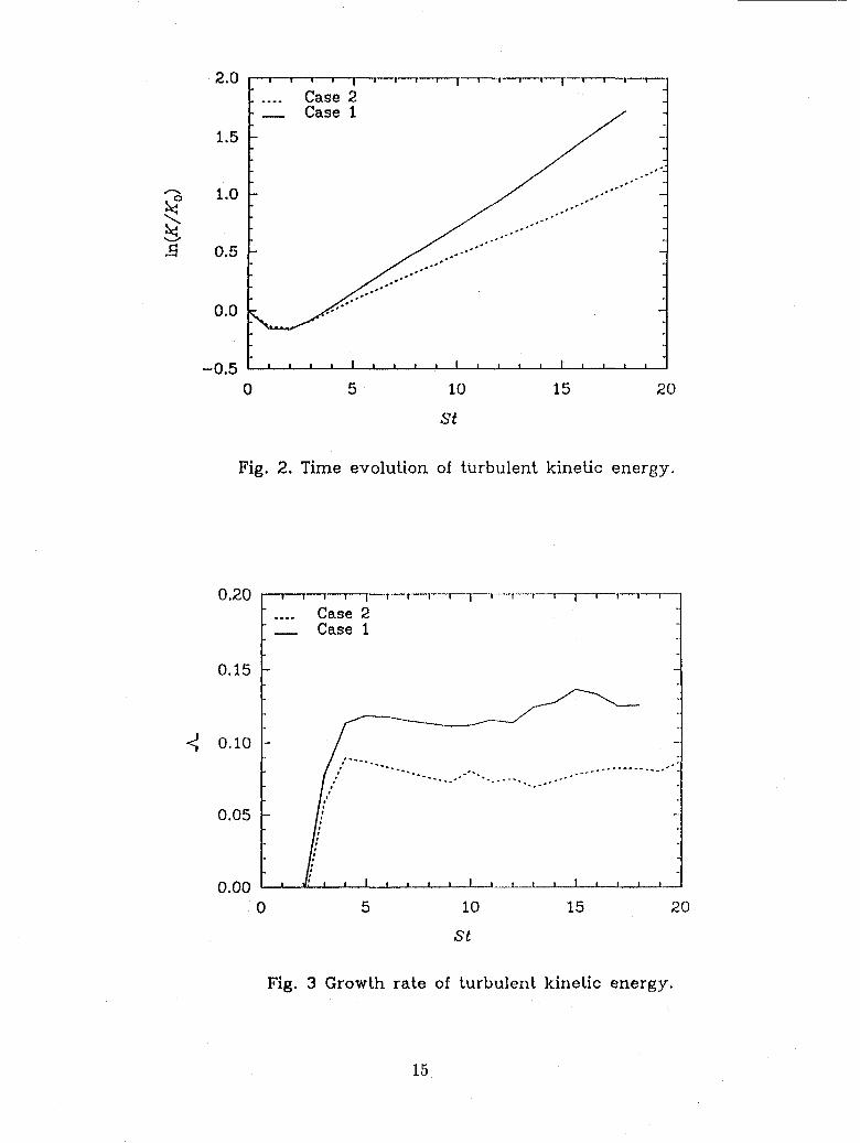
evolution of the kinetic energy K as a function of non-dimensional time St is shown in Fig. 1.
Physical experiments and DNS of the incompressible case indicate that K, after an initial
transient, evolves as K0 exp(ASt). The feature of exponential growth is carried over to the
compressible case, as evidenced by the approximately linear regime in the plot of ln(K/Ko)
in Fig. 2 for St > 7. Although the picture of exponential growth survives, the growth rate of
K shows a significant decline with a decrease in the speed of sound. Figure 3 shows that the
growth rate A = d(ln K/Ko)/d(St) decreases by about 30% when M_ increases from 0.2 to
0.4. We note that the reduction of kinetic energy growth rate with increasing compressibility
is a consistent trend in all our simulations.
In order to understand the phenomenon of reduced growth rate of kinetic energy, we
consider the equation governing the kinetic energy of turbulence in homogeneous shear whichis
d (-_K) = p--T'--_ - -Pet+ p'd-'--7 (5)
where 7_ -- co _t._ uwiwi the: solenoidal dissipation rate, cc --_,_'1_2 is the production, €8 = - _ t
(4/3)_d _2the compressible dissipation rate and p_d_ the pressure-dilatation. The last two
terms represent the explicit influence of the non-solenoidal nature of the fluctuating velocity
field in the kinetic energy budget.
If the notion of exponential growth in homogeneous shear flow is correct _,A should asymp-
tote to a constant. The relative importance of the various terms on the rhs of (5) can be
gauged by their contribution to A. We, therefore, normalize (5) by -riSK. The terms on the
rhs of (5) are plotted in Fig. 4 after being thus normalized. AccOrding to Figs. 4a-4b,the
dilatational terms are negative and reduce h. By St = 20, the combined contribution of
the dilatational terms is approximately 20% of A, implying that they need to be considered
in turbulence modeling. The normalized production, T'/SK, is plotted in Fig. 4c. The
normalized production in Case 2 begins to deviate from that in Case 1 around St = 5, and
eventua!ly asymptotes to a value noticeably smaller than in Case 1. Thus, the production is
reduced due to compressibility. The normalized dissipation in Fig. 4d also shows a decrease
in Case 2 relative to Case 1, but to a smaller degree than the production. The reduction in
growth rate of K in Case 2 relative to Case 1 seems to be primarily due to the dilatational
terms during the early phase of the evolution and, for the later phase (St > 8), is related to
a decreased level of production.
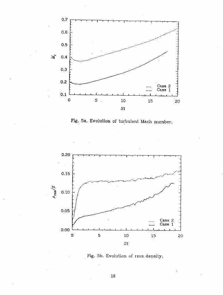
3.2 Measures of Compressibility
Apart from the differences in the evolution of turbulence statistics in the case of compressible
flow relative to incompressible flow, a question that arises is how compressible is the turbu-
lence? The turbulent Mach number Mt = _/_ and the normalized rms density P_ms/'_are
measures of departure from incompressibility, since both these quantities are zero for strictly
incompressible flow. Mt shows a monotone increase in Fig. 5a reaching a maximum of 0.6,
which•is larger than the upper bound of Mt in free shear layers and wall boundary layers
encountered in aerodynamic practice. Figure 5b shows that, after starting from zero density
fluctuations, both simulations develop significant rms density levels at St = 18, and most of
the increase in rms density occurs rapidly within St < 3 for Case 2 (with the higher initial
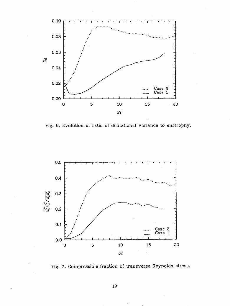
Mr). The velocity field is no longer solenoidal in compressible flow, that is, d = V.u _ 0. Forhomogeneous flow, the Helmholtz decomposition gives a unique decomposition of the veloc-
ity field into incompressible and compressible components by u = u I + u c, where V. ut = 0
and V × u C = 0. The departure of the velocity field from solenoidality is another measure
of compressibility, and can be represented by the ratio of dilatational variance to enstrophy
Xd = d /w_w_or by the fraction of kinetic energy which is dilatational XK --_ Kc/K. The for-
mer quantity Xd is more general, because the Helmholtz decomposition required for obtaining
Kc is unique only for homogeneous flows. Figure 6 shows that after an initial transient, Xd
increases monotonically for Case 1, but levels off at about 8% for Case 2. The quantity XK
(not plotted here) is comparable to Xd, leveling off at approximately 6% for Case 2. Since
the mean shear leads to anisotropy of the Reynolds stress tensor, the dilatational fraction
of each Reynolds stress component is obtained. Except for the transverse component I '_2_2,
the dilatational contribution to the Reynolds stress tensor was a few percent, comparable tothe magnitude of XK. The ratio of _c,^ c,, ,_,_2 _2 /_2'_2 is substantially larger, as shown in Fig. 7.
Since the dilatational component i_ a relatively poor mixer of scalar compared to the vortical
component, the large ratio of o_2C'o_2Cr/o/_,.2'° ' implies that mixing is preferentially decreased bycompressibility in the direction of shear.
3.3 Compressible and Solenoidal Spectra
The Fourier component of the velocity is decomposed into components perpendicular and
parallel to the wave number vector from which the solenoidal spectrum E,(k) and com-
pressible spectrum E_(k) are calculated. Figure 8 compares the solenoidal and compressible
spectra at St=15 (when Mt = 0.55) for Case 2. The compressible energy is small relative to

the incompressible energy for all modes. The compressible spectrum is flatter at low wave
numbers (/c < 16) relative to the incompressible spectrum. The two spectra have similar
slopes in the intermediate wave number range. The solenoidal spectrum is compared in Fig. 9
between an incompressible run (Mr = 0) and a compressible run at St = 17. The compress-
ible run has an initial Mt of 0.4 and the initial velocity and pressure fields are the same as in
the incompressible run. LFrom Fig. 9, it appears that the shape of the solenoidal spectrurri is
not altered by compressibility, even though the compressible fluctuations are non-negligible
at this time- P_ms/-fi= 0.12 and Xk = Kc/K = 0.05. However, the pressure spectrum in
Fig. 10 shows significant differences between these two cases. In the compressible case, the
pressure spectrum seems to be relatively flatter than in the incompressible case.
4 Modeling the Dilatational Terms
We showed in Fig. 4 that the compressible dissipation _c and the pressure-dilatation p_d---7
contribute significantly to the kinetic energy budget and therefore require modeling. In
Sarkar et al. (1991), we proposed a model for the compressible dissipation cc = alcsM_ based
on an asymptotic analysis and DNS of isotropic turbulence. In the present simulations, after
starting from a variety of initial conditions, _ __ 0.5_sMt2, suggesting that al = 0.5.
Our direct numerical simulations of isotropic turbulence and homogeneous shear flow
provided a data base for the pressure-dilatation and suggested a theoretical approach towards
modeling it. The evolution of the pressure-dilatation ptd_ for Case 1 is depicted by the solid
curve in Fig. 11. $From numerical experiments, it was found that the nominal time period
of the oscillations in p_d_ decreased approximately linearly with the speed of sound. This
suggested that one could isolate the oscillatory part of p_d"---i by decomposing the fluctuating
pressure p_ into the sum of an incompressible part p,r_ and a compressible part pC_. The
incompressible pressure p_ satisfies
v2p --= - - j (6)
while the remainder pet is the compressible pressure. The rhs of (6) collects all terms that
depend on _ in the equation obtained by taking the divergence of the momentum equation.
In the simulations, since pt is available from the compressible Navier-Stokes solution and
pI_ is evaluated from (6), we obtain pC_ as the difference pt _ pI _. Since p_ = p I_ + pC_ we
have p_d_ = pI'dt + pC'dq The oscillations are substantial only for pC'd_ (dotted curve in
Fig. 11), and furthermore, the peaks and valleys in the evolution of pe'd_ seem to be much
more symmetric around the origin than those in p_d' (solid curve in Fig. 11). The component
pI'd_ (dash-dotted curve in Fig. 11) does not have strong temporal oscillations, and shows
a systematic decrease with time. In order to gauge the relative importance of the two
components pC,d' and pI,d' of the pressure-dilatation in the evolution of the turbulent kinetic
energy, we calculate the time integrals of these components. The integrated contribution of
pX'd' is about an order of magnitude larger than that of pC'dr in Case 2. Examination of
other DNS cases indicates that, in general, pC,d' has a negligible contribution to the turbulent
kinetic energy evolution relative to pI'd'. Therefore. it seems that only the component pI'd'of the pressure-dilatation requires modeling in shear flows.
In order to model pI'd', we consider the Poisson equation (6) for the incompressibleS I
pressure. After splitting the pressure into a rapid part pn' and a slow part p , we obtain the
following exact expressions for the rapid pressure-dilatation and slow pressure-dilatation:
pn'd' = f _E_idk (7)
pS'd7= -_ kmk_kd . .__,,̂ ,k2 (zuludu m -- iu_d*_tm) dk (8)
Here €* denotes the complex conjugate of the Fourier transform € and End represents the
spectrum of the Reynolds stress tensor ' 'u_uj. Using scaling arguments (see Sarkar (1991) for
details) to simplify (7)-(8) we find that pn'd' depends on the production 7) while pS'd' depends
on the dissipation €8. Finally, we propose the following model for the pressure-dilatation:
8 2p'd' = a2"fi_t_,jb_jq2Mt + aa'ficsM2t+ -_-fi_t_,_x(Mt )q (9)
where blj . ,,. ,,1_2 5ij/3 is the anisotropy tensor, Mt _/_ the turbulent Mach= 'tti'uj/q --
number, and _ the solenoidal dissipation. To obtain the functional dependence x(Mt) in
the last term of Eq. (9), one would require data from a flow with mean homogeneous com-
pression. In this paper, we validate and calibrate the first two terms in the model for p'd'.In homogeneous shear, the model becomes
p'd' = -a2p-p-_Mt + a3-_e_M_ (10)
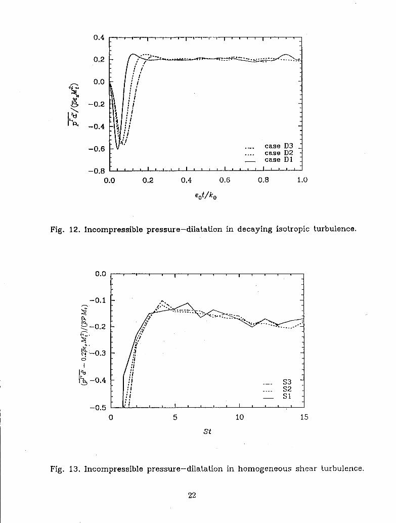
where 7) = -Su"u"l2. Because the production 7) = 0 in decaying isotropic turbulence, the
variation of the incompressible pressure-dilatation with €, can be verified using DNS of
isotropic turbulence. The ratio pI'd'/(-_,M_) is shown as a function of non-dimensional
time in Fig. 12. The decaying isotropic turbulence simulations, D1,D2 and D3 start with
Mt,o of 0.6,0.5, and 0.4 respectively, p_'d'/(-_€,M_) reaches an equilibrium value by a time
of 0.25, substantiating the validity of the second term in (9). Based on the DNS value of
the equilibrium ratio, the model coefficient a3 in (9) is taken to be 0.2, The remaining part
of the model for the pressure-dilatation is calibrated against simulations of homogeneous
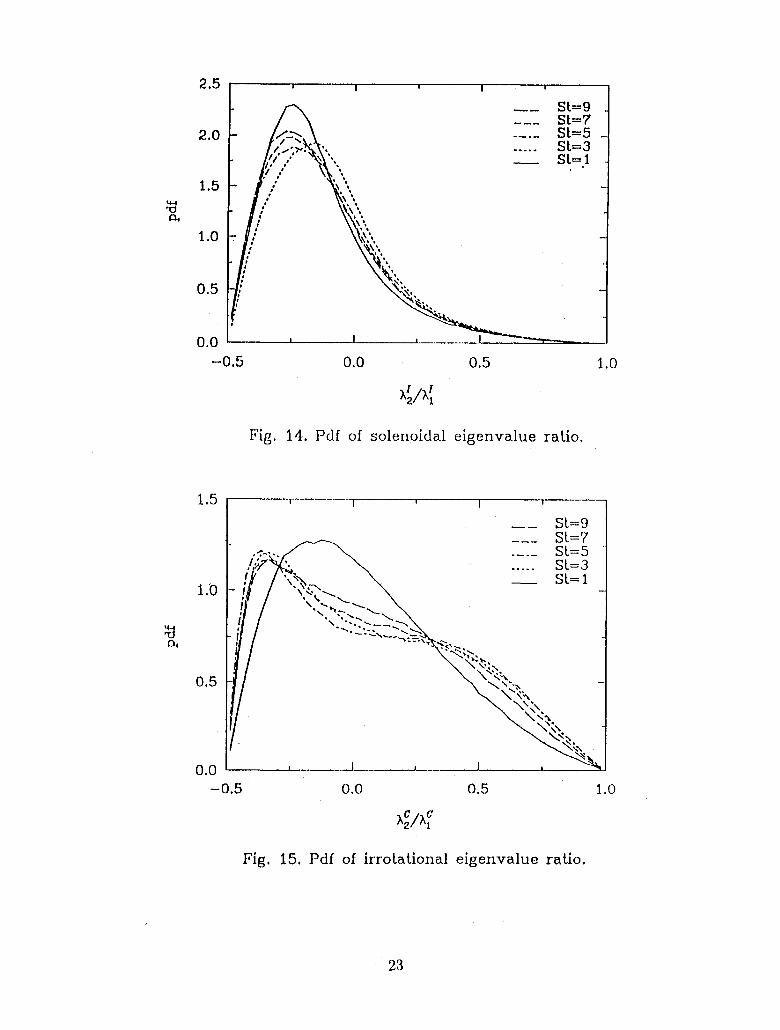
shear flow. Fig. i3 shows results from three cases $1,$2 and $3 with Mt,o of 0.2,0.3, and
0.4 respectively. Cases $2 and $3 have shear S=15, while Case $1 has S=20. After St = 5,
the ratio (p1'd' - 0.2-ficsMt2)/(-fiPMt)evolves in a similar fashion for the three cases and
exhibits a slight decrease with time. In the period 5 < St < 15, the three cases $1-$3
encompass a range of turbulent Mach numbers of 0.21 < Mt < 0.65. The results of Fig. 13
suggest that, with a coefficient a2 = 0.15, the proposed model (9) is able to parametrize thepressure-dilatation for 0.2 < Mt < 0.6.
5 Structure of the Rate of Strain Tensor
In this section, we study several properties of the rate of strain tensor Sij to help identify
characteristics of the flow which are solely the result of compressibility effects, and how
these characteristics differ from corresponding properties in an incompressible turbulent flow.
Because the flow is anisotropic, it is useful to consider characteristics of the flow both with
respect to the laboratory frame of reference, and with respect to a frame of reference attached
to, and rotating with an individual fluid element. Global orientation properties of Sij are
established by studying the principal directions of Sij in the laboratory frame of reference.
(In isotropic turbulence, this diagnostic does not provide useful information.) On the other
hand, local properties can be characterized by considering the relative orientation of vectors
such as velocity, vorticity or scalar gradients, with respect to the principal directions of Sij.
We consider the rate of strain tensor, decomposed according to
S_j = S .c. S t.. 1,_ + ,_ + _ u_,_6ij (11)
where S/j and S_j are respectively constructed from the solenoidal and compressible (irrota-
tional) velocities u I and u c. Both S{j and S_j are deviatoric. The properties of these tensors
are expressed in terms of invariant quantities, i.e. eigenvalues and eigenvectors. Because S_j
is symmetric, its eigenvalues Ai, i = 1, 2, 3 are real, and its eigenvectors are in the directions
of maximal or minimal extension (depending on the signs of the Ai) of the tensor. These
directions are given by the tensor's three eigenvectors. For future reference, the eigenvalues
are ordered from smallest to largest:
A1 < A2 < _3. (12)
The first three invariants of the tensor Sij, defined as the coefficients of the polynomial
characteristic equation, are related to small scale phenomena, and can be expressed in terms
of the eigenvalues. These relationships are:
I = -(AI+A2+A3)
8
II = _1_2 + _1_3 + ,_2A3
III= -/_1 _2 _3
If the tensor is deviatoric, I = 0, -II = SijSji which for incompressible flow is proportional
to the dissipation, and in isotropic flow, III is proportional to the third moment of the
velocity gradient probability distribution function (pdf).
We present results from one simulation with S = 15, and/_ = 1/150, M,0 = 0.3, Rm = 20
and incompressible initial data. The simulated flow is analyzed at St = 1, 3, 5, 7, 9, which
are all sufficiently resolved. More details of this analysis can be found in Erlebacher, Sarkar
and Hussaini (1991). Note that all the pdf's that follow are unconditioned and unweighted.
Sampling for the pdf's (probability density function) is done on a grid resolution of 48 x96 x96
although the simulation was performed on a 963 mesh. This provides over 400,000 sample
points.
The pdf of I I c 6'_2/)_1 areA2/A1 and shown in Figs. 14 and 15. Both plots show that
after an initial transient, the eigenvalue ratios have single peaks. These are located at -
0.25 for the solenoidal ratio, and at approximately -0.375 for the irrotational ratio. As a
consequence, the rate of strain tensors S/j and S_, respectively, have preferred strains in the
A2/A1 withratios (-4 : 1 : 3) and (-8 : 3 : 5) along the principal axes. Conditioning of I x
respect to _, sharpens the peak for higher values of dissipation. Further processing of the
irrotational ratio distribution is underway. A check of the pdf of the irrotational ratio was
also performed from a 1283 database (Case 2) with 800,000 sample points, and its shape
is qualitatively similar with the peak at -0.375. Note that the pdf of the irrotational ratio
is more broadband than that of the solenoidal ratio. However, the location of the peak is
well defined, and constant in time. This equilibrium structure of (-4 : 1 : 3) for Sij is
observed in incompressible flow, first by Ashurst, Kerstein, Kerr & Gibson (1987). They_I2 x Iconsidered the statistics of (2) /(S_jS_j) conditioned on the dissipation and found that the
preferred ratio was most dominant in regions of high dissipation. In a later work, Chen et
al. (1990) displayed scattergrams of II versus III based on incompressible mixing layer
DNS data, which clearly demonstrated that III is proportional to (-II) 3/2 in the regions of
highest dissipation. This is in fact a statement about the preferred shape of the S/j principal
ellipsoid. Our results indicate that compressibility does not substantially affect this preferred
structure of the solenoidal S/j.
The distribution of _ and _ show some distinctive differences, as illustrated in Figs.
16-17. Both figures show negative skewness of the distributions, and a flattening in time,
although the effect is much more severe for A_. On both plots, the most probable value
for the eigenvalue shifts towards more negative values. In the irrotational case, the effect
is extremely strong. However, the most probable ratio of ,_ to A1C(see Fig. 15) remains
9
invariant in time. Figure 17 also indicates that the amount of change in the distribution of
A_ decreases with time, but there is no strong evidence that the shape of the pdf is evolvingtowards a steady state.
Information on structural differences in the flow as they relate to preferred directions of
straining for both the solenoidal and dilatational components of the flow are presented next.
After the eigenvectors of the rate of strain tensors are normalized to unity, we compute the
angle 0_jbetween eigenvector f_ and the unit vector in the coordinate direction xj. The pdf's
of Icos0i§[ and Icos0_l are then computed. The cosine of 0 is chosen instead of 0 so that
the probability density function based on a Gaussian distribution for the velocity derivatives
is flat. In Figs. 18-19, we respectively plot the pdf of Icos01Ziland Icos01_l, (i = 1,2,3) atSt = 9 to illustrate that the solenoidal and irrotational rate of strain tensors have different
preferential alignments in the laboratory frame of reference. Note that R_ = 33 at this time.
The direction of maximum compression of S_ (f[) tends to be at approximately 45° to both
the x and y axes, with no preferred orientation with respect to z. The alignment of faI is also
in the 45° direction, while f_ has no unambiguous preferred direction. The irrotational rate
of strain tensor exhibits markedly different properties. Most of the distributions of cos 0ij
have two strong peaks, thus indicating two preferred directions of alignment. For example,
f_ is most often aligned along one of the thr(c, coordinate axes. This is true of the other
two principal directions, but to a lesser degree. Interestingly enough, all three pdf's of f_
exhibit a valley in the neighborhood of 45°. Statistics based on the database of Case 2 (at a
higher shear and higher Reynolds number than the results plotted in the preceding figures)
show that the pdf's of [cos 0_i[ and [cos 0_[ are sharper. In particular, the tendency for f_ to
align is strongest in a direction at 30° to the x axis and not 45°. Finally, we notice that all
the pdf's of [cos 0ij[ tend towards a steady distribution with increasing St. The distribution
of [cos0_[reachesan equilibriatedstageat a muchearlierstage than does [cos 0_[.
6 Conclusions
We have performed DNS of homogeneous shear using a 128a grid to ascertain the influence of
compressibility on turbulence statistics and structure. The primary result is the stabilizing
effect of compressibility on the growth of kinetic energy. We find that the reduction in
growth rate is due to the pressure-dilatation and compressible dissipation acting as sinks for
the kinetic energy, and due to the reduced level of the Reynolds shear stress. After starting
with zero density fluctuations, the simulations develop significant density fluctuations and
moderate levels of energy in the dilatational component. The dilatational velocity component
is strongly anisotropic, and consequently its contribution to the transverse rms velocity is
10

much larger than to the other rms turbulent velocities. AlthOugh, the turbulent Mach number
and rms density fluctuations are significantly large, the shape of the energy spectrum is
practically unaffected by compressibility. However, the pressure spectrum is much flatter for
the compressible case relative to the incompressible case. The eigenvalues and eigenvectors
of both the solenoidal and irrotational rate of strain tensors were examined for preferred
structure. In principal axes, the solenoidal rate of strain tensor has a preferred shape of (-
4:1:3) in accord with previous results available for incompressible flow. The irrotational rate
of strain tensor has a different preferred shape. The pressure-dilatation correlation needs to
be modeled for compressible flow. We consider a form of the pressure equation obtained by
taking the divergence of the momentum equation, deduce a formal solution for the pressure-
dilatation, and then simplify to obtain a model for the pressure-dilatation. The model seems
to compare well with DNS data in isotropic turbulence and homogeneous shear turbulence.
11
References
[1] Ashurst, Wm. T., Chen, J.-Y.,and Rogers, M.M.: Pressure Gradient Alignment with
Strain Rate and Scalar Gradient in Simulated Navier-Stokes Turbulence.Phys. Fluids A,
30, (1987a) 3293-3294.
[2] Ashurst, Wm. T., Kerstein, A.R., Kerr, R.M., and Gibson, C.H.: Alignment of Vorticity
and Scalar Gradient with Strain Rate in Simulated Navier-Stokes Turbulence. Phys. Fluids
30, (1987b) 2343-2353.
[3] Blaisdell, G.A., Mansour, N.N, and Reynolds, W;C.: Numerical simulation of Compress-
ible Homogeneous Turbulence, Stanford University Report No. TF-50 (1991).
[4] Chen, J.H., Chong, M.S., Soria, J., Sondergaard, R., Perry, A.E., Rogers, M., Moser,
R., and Cantwell, B.J.: A study of the topology of dissipating motions in direct numer-
ical simulations of time-developing compressible and incompressible mixing layers. CTR,
Proceedings of Summer Program (1990).
[5] Coleman, G.N., and Mansour, N.N.: Modeling the rapid spherical compression of
isotropic turbulence. Phys. Fluids A,3 (1991) 2255-2259.
[6] Erlebacher, G., Hussaini, M'Y., Kreiss, H.O., and Sarkar, S.: The Analysis and Simula-
tion of Compressible Turbulence. Theoret. Comput. Fluid Dynamics, 2 (1990) 73-95.
[7] Erlebacher, G., Sarkar, S., Hussaini, M. Y.: Structure of Compressible Turbulence in
Homogeneous Shear Flow. ICASE Report (in preparation).
[8] Feiereisen, W.J., Shirani, E., Ferziger, J.H., and Reynolds, W.C.: Direct Simulation of
Homogeneous Turbulent Shear Flows on the Illiac IV Computer. In Turbulent Shear Flows
3 (1982) 309-319. Springer-Verlag, Berlin.
[9] Kida, S. and Oszag, S.A.: Energy and Spectral Dynamics in Forced Compressible Tur-
bulence. J. Sci. Comp., 5, (1990) 85.
[10] Lee, M.J., Kim, and J., Moin, P.: Structure of turbulence at high shear rate. J. Fluid
Mech., 216, (1990) 561-583.
[11] Lee, S., Lele, S.K., and Moin, P.: Eddy-shocklets in Decaying Compressible Turbulence.
CTR Manuscript 117(1990).
[12] Passot, T.: Simulations numeriques d'ecoulements compressibles homogenes en regime
turbulent : application aux nuages moleculaires. Ph.D. Thesis, University of Paris (1987).
12
[13] Rogallo, R.S.: Numerical Experiments in Homogeneous Turbulence. NASA TM 81315
(19Sl).
[14] Rogers, M.M., and Moin, P.: The Structure of the Vorticity Field in Homogeneous
Turbulent Flows. J. Fluid Mech., 176 (1987) 33-66.
[15] Sarkar, S., Erlebacher, G., Hussaini, M.Y., and Kreiss, H.O.: The Analysis and Model-
ing of Dilatational Terms in Compressible Turbulence. J. Fluid Mech, 227 (1989) 473-493.
[16] Sarkar, S., Erlebacher, G., and Hussaini, M.Y.: Direct Simulation of Compressible
Turbulence in a Shear Flow. Theor. Comput. Fluid Dyn., 2 (!991) 291-305.
[17] Sarkar, S.: Modeling the Pressure-dilatation Correlation. ICASE Report 91-42 (1991).
[18] Vieillefosse, P.: Internal Motion of a Small Element of Fluid in an Inviscid Flow. Physica
125 A,(1984) 150-162.
[19] Zang, T.A., Dahlburg, R.B., and Dahlburg, J.P.: Direct and Large-eddy Simulations of
Compressible, Isotropic, Navier-Stokes Turbulence. Phys. Fluids A (in press).
13
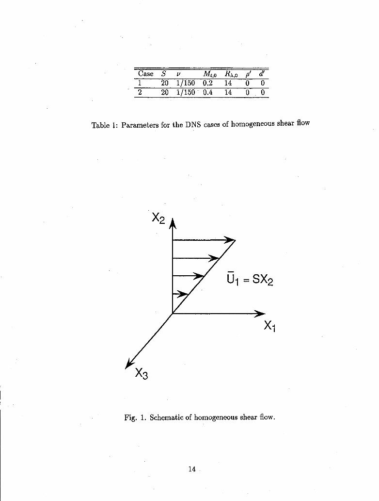
Case S v M_,o Rx,o p' d_1 20 1/150 0.2 14 0 02 20 1/150 0.4 14 0 0
Table 1: Parameters for the DNS cases of homogeneous shear flow
X2 lk
._,
= SX 2
Fig. 1. Schematic of homogeneous shear flow.
14
_.0 ' ' ' ' I ' ' ' ' I ' ' ' ' I ' ' i , ,
....Case2Case1
1.5
1.00.5
0.0
--0.5 i , , , I , , , , I , , , , I , , , ,
0 5 i0 15 20
st
Fig. 2. Time evoluUon of turbulent kinetic energy.
0._0 ' ' ' _....I ' ' ' ; I _ ' ' ' I ' ' ' '.... Case 2__ Case I
0.15
<_ 0.I0
0.05 ....,'!0.000 5 I0 15 20
St
Fig. 3 Growfh rate of turbulen[ kinetic energy.
15
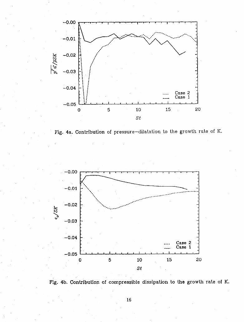
Fig. 4a. Cont,ribution of pressure-dila[ation to [he grow[h rat.e of K.
-0.00 ' , ' ' , .... I ' ' ' ' , ' ' ' ''-
-0.01 "',,", ....-.....--...... .
...... .--'"..-', .oo°
-0,02 --"",.. .... °.-_°°
-0.03 -
-0.04....Case2__ Case1
-0.05 , , , , i , , , , l .... t , , , ,0 5 I0 15 20
St
Fig, 4b. Conbibution of compressible dissipation to the grow[h rate of K.
16

0.4
0.3
0.2
0.I
...... Case 2 "Case i "
0.00 5 10 15 20
S_
Fig. 4c. Contribution of production to the growth rate of K.
0.30
.... Case 2Case i
0.25
0.15
0.100 5 10 15 20
St
Fig. 4d. Contribution of solenoidal dissipation to the budget of K.
17
0.7Ill'l|Jll;flll;ia,;,
0.6 ..... "')ooo o°°
.oo°
o...o°"
0.5 ........
_ 0.4.
0.3
0.2.... Case2
Case 1
0 5 10 15 20
St
Fig,5a,Evolutionof turbulentMach number.
0.20
0.15
J'_ 0.10
0.05
0.00
0 5 10 15 2O
St
Fig.5b.Evolutionofrms density.
18
0 10o " w " l T ' 'I I ' '| W ! ! _ I ' ! l ! _ W 'I" € |
0.08 "..................................... 'e
0.06 /
0.04
0.02.... Case 2__ Case 1
0.00 .... I ..... J .... i .....0 5 10 15 20
St
Fig. 6. Evolution of ratio of dilatational variance to ensbophy.
,5 ww'wv|'v"v"l''"''v'|_wm'v
0.4 o,, ,......,s_° _.°. ..... •
s'
0.3am
wo
I_ 0.2 ,.
0.1 // 2
.iJ __. Case i0.0 ' ' ' I , , , , ! , , , , I , , , ,
0 5 10 15 20
St
Fig. 7. Compressible fraction of transverse Reynolds stress.
19

Fig. 8. Energy specLra at S_--15 for Case 2.
........0 ' '.-'" ' "_.'.-o,1.. , " ,'" , , ' ' | ,' ' _ ,_o.o ! ....
-3 _ ",,,';
-4 'Incompressible caseCompressible case
-5
0.5 1.0 1.5 2.0
log(k)
Fig. 9. Solenoidal velocity spectra for compressible and incompressible runs.
20

"Ias_Du!uo.rl_l_i!p-a_nssaidIoUo!]nlOAH"II'_l!zI
gI01:
i,i,,,,i,,,,9-_,-
"%,_--
•/
,,,,,,.:'0
,ti,,,li,,j
•sunlalq!ssa_duloou! pu_alq!ssaIduloo _oI_.qoadselnssaId'Of"_[.,1"
O'g_'_O'I_'0
__,,,,,,,,,,,,\as_oalq!ssa_duloD
•.
i|II]IIiIiIPii
-60.5
2
o
-4
'" ......... ..................... -..... ~ ........
........... '.
Incompressible caseCompressible case
1.0
log(k)
1.5
.................
2.0
Fig. 10. Pressure spectra for compressible and incompressible runs.
4
.":~ .\ ;:. :: ,.I ,t ,I
I' ::
':
2
o
-2
-4
-65 10
st
......., ,: ~ I, "
"",
I
""",-""", ,, .,.,,, ,.,
"...'-: ~:
.'
15
Fig. 11. Evolution of pressure-dilatation in Case 1.
21
0.4 i_ ' ' ' ' I ' ' i, , 1 ' ' ' ' I ' ' ' ' I ' ' ' ' '
Lo2I_ __-__
/,'/Iii
0.0_- I;i
'Iii-0.2
-0.4 ,_,,I-t;d : l
-0.6 I _f_'! ._. case D3
case D2case D 1
--0.8 [ I I , , I _ I , , I , , , , I , , , , I , , , ,
0.0 0.2 0.4 0.6 0.8 1.0
%t/ko
Fig. 12. Incompressible pressure-dilatation in decaying isotropic turbulence.
0.0 ' ' ' ' ! ' ' ' ' I ' ' ' '
-0.1
<-0.2 " "_" ""
_. -0.3CD
I
-o.4 l i_-- s3I:',' .... s2:Ii_ __ sl
-0.5 , ! , , , I .... I , , , ,0 5 10 15
St
Fig. 13. Incompressible pressure-dilatation in homogeneous shear turbulence.
22
_.5 ' I ' I '
St=9/_ Y-- st=_
2.0 /.<'._>.\ .... St=5//., "..';._'X',, . .... St=3
'°t- 'o_!" _%0.0 '
-0.5 0.0 0.5 1.0
! IX2/X,
Fig. 14. Pdf of solenoidal eigenvalue ratio.
1.5 ' I ' I '
__ St=9___ St=7.... S1=5..... S1=3
1.0 SL=1
:U "'.bO4
0.0 I , I
-0.5 oo o_ lo
Fig. 15. Pdf of irrotational eigenvalue ratio.
23
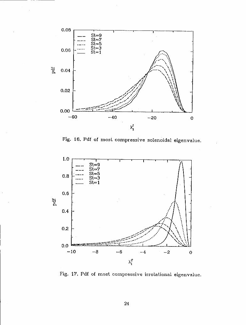
0.08 i i___ St.=9___ S1.=7.... St.=5
0.06 ..... St.=3
IS./>.- -,,,. \ ;
0.04 /'-",2,',;
0.02 ×/,,.,;.1 \"I ./oo*
0.00 - ' .... _ , I ,
-60 -40 -20 0
Fig. 16. Pdf of most compressive solenoidal eigenvalue.
1.0 i iSt.=9St.=7S!.=5
O.B St.=3Sl.= 1
Fig. 17. Pdf of most compressive irro(ational elgenvalue.
24

_.0 ._._' _ X3! ..... ' ! ' I ...... ' I _ ]
..... :1_3:2
1.5 _ 1
m_ 1.0 .... ..^._..<r_. .,i ,°. , • N,
0.5
0.0 ' , , I , ,, , I , I t I t J
0.0 0.2 0,4 0.6 0.6 1.0
Ic°sO_,l
Fig. 18. Pdf of the orientaLion of [he mosL compressive
solenoidal eigenvecLor wiLh respect Lo Lhe three coordinaLe axes.
Fig. 19, Pdf of Lhe orienLaLionof Lhe mosL compressiveirrofafional eigenvecLor wiLh respecL Lo [he [hree coordJnafe axes.
25

Form ApprovedREPORT DOCUMENTATION PAGE oMB_oo7o4-o188
PuDhc reoortlng burden _o" _h,s:oliectlon of reformation ,s estimated to avera,3e ; nout #er -espoase, mcludlnQ the time for reviewing instructions, searching exlstmd data sources,gathermq and maintaining the data needed, and comoleting and revlewlr, c the _'ohe_lon of Informat on Send'comments re ard ng th sburden est mate or any other- aspect of th;S_oNe(tlor_ of information, ,ncbudlng suggestions for reducing this Ouroen, t'o v'Casnmgton _eaaquarters Serv,ces, Directorate _o_rInformation Ooeratlons and Reports. 1215 JeffersonDavis Highway Suite 1204, Alilnqton VA 22202-4302 and to the Off (e of Manaqernent and Budget. Paperwork Reduction Prolect (0704-0188), Washington, DC 20503.
1. AGENCY USE ONLY (Leave blank) I 2. REPORT DATE 3. REPORT TYPE AND DATES COVERED
I February 1992 Contractor Report4. TITLEAND SUBTITLE 5. FUNDINGNUMBERS
COMPRESSIBLE HOMOGENEOUS SHEAR: SIMULATION AND MODELING C NASI-18605
6.AUTHOR(S) WU 505-90-52-01
S. Sarkar, G. Erlebacher, and M. Y. Hussaini
'7. PERFORMINGORGANIZATIONNAME(S)ANDADDRESS(ES) 8. PERFORMINGORGANIZATIONInstitute for Computer Applications in Science REPORTNUMBERand Engineerlng
Mail Stop 132C, NASA Langley Research Center ICASE Report No. 92-6Hampton, VA 23665-5225
9. SPONSORING/MONITORINGAGENCYNAME(S)AND ADDRESS(ES) 10.SPONSORING/MONITORING
National Aeronautics and Space Administration AGENCY REPORTNUMBER
Langley Research Center NASA CR-189611
Hampton, VA 23665-5225 ICASE Report No. 92-6
11.SUPPLEMENTARYNOTES
To appear in 'Turbulent ShearLangley Technical Monitor: Michael F. CardFinal Report Flows 8: Selected Papers' (1992
12a. DISTRIBUTION/AVAILABILITYSTATEMENT 12b,DISTRIBUTIONCODEUnclassified - Unlimited
Subject Category 34
13. ABSTRACT(Maximum200words)
The present study investigates compressibility effects on turbulence by direct numer-
ical simulation of homogeneous shear flow. A primary observation is that the growthof the turbulent kinetic energy decreases with increasing turbulent Math number.
The sinks provided by compressible dissipation and the pressure-dilatatlon, along
with reduced Reynolds shear stress, are shown to contribute to the reduced growth of
kinetic energy. Models are proposed for these dilatational terms and verified by
direct comparison with the simulations. The differences between the incompressibleand compressible fields are brought out by the examination of spectra, statisticalmoments, and structure of the rate of strain tensor.
!4. SUBJECTTERMS 15. NUMBEROF PAGES
compressible flow, turbulence 2716. PRICECODE
A03
17. SECURITYCLASSIFICATION! 8. SECURITYCLASSIFICATION19, SECURITYCLASSIFICATION 20. LIMITATIONOFABSTRACTOFREPORT OFTHISPAGE OFABSTRACT
Unclassified Unclassified
NSN7540-01-280-5500 Standard Form 298 (Rev 2-89)PrescrlbeG Oy ANS Std z3g-18298.102
NASA-Langley, 1992


1I1111"1111"lllif,ijIIJijr~rtll~1 ~'If(li~IIIIIIIIII"11113 1176014168943
Ijjjjjjjjj
. j
jjjjjjjjjjjjjjjjjjjjjjjjjj
Top Related