Download - Multivariate ANOVA - Jonathan Templin's Website · Overview ANOVA Example Hungry? Can You Guess? SAS Code MANOVA One-Way MANOVA Example Treatment CIs Two-Way MANOVA Two-Way …

Lecture #5 - 7/26/2011 Slide 1 of 47

Multivariate ANOVA

Lecture 5July 26, 2011

Advanced Multivariate Statistical MethodsICPSR Summer Session #2

Overview

● Today’s Lecture

ANOVA Example

MANOVA

One-Way MANOVA Example

Treatment CIs

Two-Way MANOVA

Two-Way MANOVA Example

Wrapping Up

Lecture #5 - 7/26/2011 Slide 2 of 47

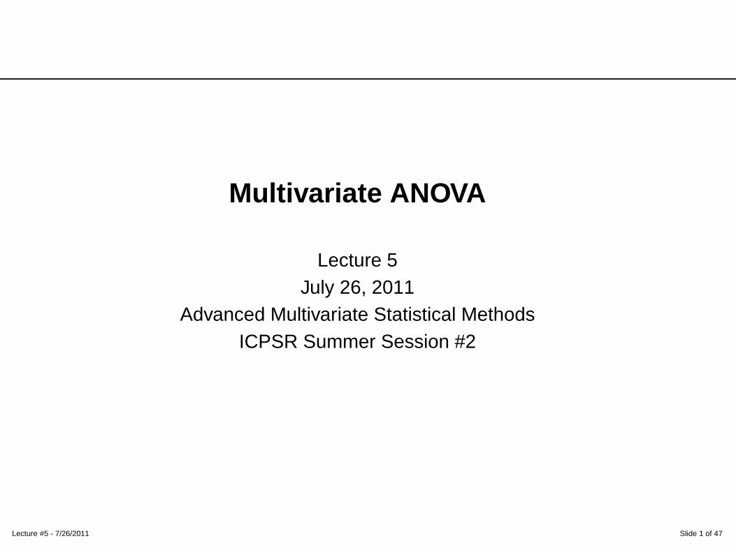
Today’s Lecture

■ Univariate ANOVA Example

■ Multivariate ANOVA (MANOVA)

◆ One-way MANOVA

◆ Two-way MANOVA

Overview

ANOVA Example

● Hungry?

● Can You Guess?

● SAS Code

MANOVA


Treatment CIs

Two-Way MANOVA


Wrapping Up

Lecture #5 - 7/26/2011 Slide 3 of 47

Setup

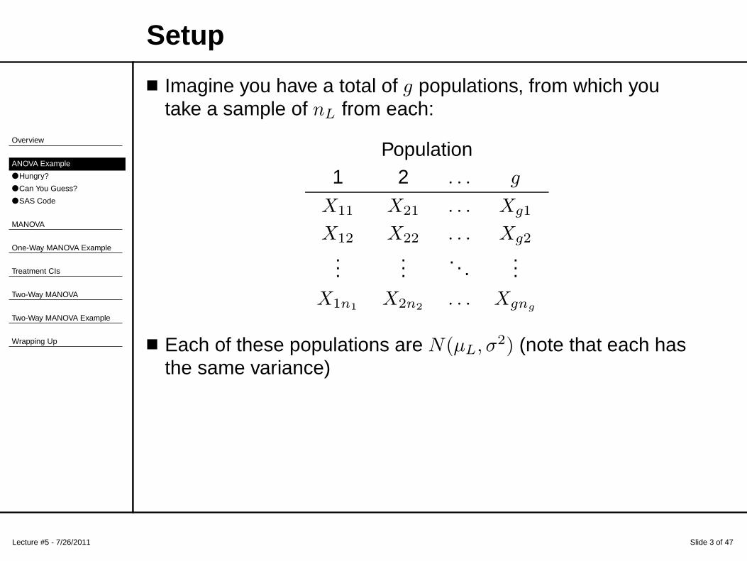
■ Imagine you have a total of g populations, from which youtake a sample of nL from each:

Population1 2 . . . g

X11 X21 . . . Xg1

X12 X22 . . . Xg2

......

. . ....

X1n1X2n2

. . . Xgng

■ Each of these populations are N(µL, σ2) (note that each hasthe same variance)

Overview

ANOVA Example

● Hungry?

● Can You Guess?

● SAS Code

MANOVA


Treatment CIs

Two-Way MANOVA


Wrapping Up

Lecture #5 - 7/26/2011 Slide 4 of 47

Hypothesis Test

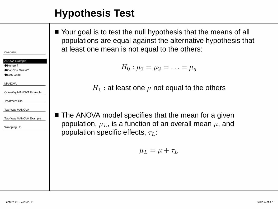
■ Your goal is to test the null hypothesis that the means of allpopulations are equal against the alternative hypothesis thatat least one mean is not equal to the others:

H0 : µ1 = µ2 = . . . = µg

H1 : at least one µ not equal to the others

■ The ANOVA model specifies that the mean for a givenpopulation, µL, is a function of an overall mean µ, andpopulation specific effects, τL:

µL = µ + τL

Overview

ANOVA Example

● Hungry?

● Can You Guess?

● SAS Code

MANOVA


Treatment CIs

Two-Way MANOVA


Wrapping Up

Lecture #5 - 7/26/2011 Slide 5 of 47

Parameterization

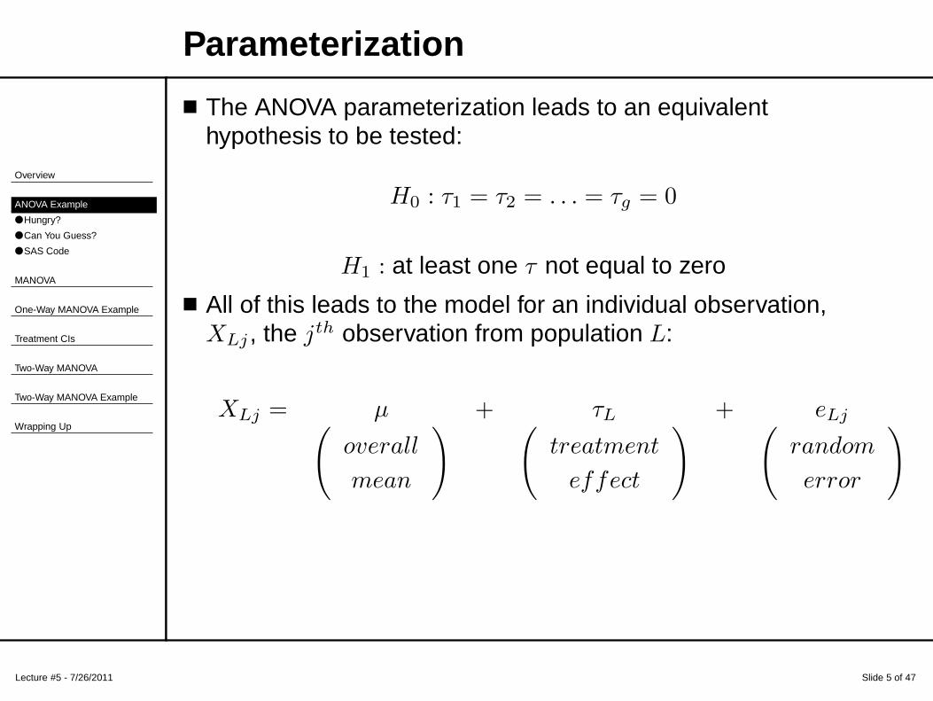
■ The ANOVA parameterization leads to an equivalenthypothesis to be tested:

H0 : τ1 = τ2 = . . . = τg = 0

H1 : at least one τ not equal to zero

■ All of this leads to the model for an individual observation,XLj , the jth observation from population L:

XLj = µ + τL + eLj(

overall

mean

) (

treatment

effect

) (

random

error

)

Overview

ANOVA Example

● Hungry?

● Can You Guess?

● SAS Code

MANOVA


Treatment CIs

Two-Way MANOVA


Wrapping Up

Lecture #5 - 7/26/2011 Slide 6 of 47

How ANOVA Works

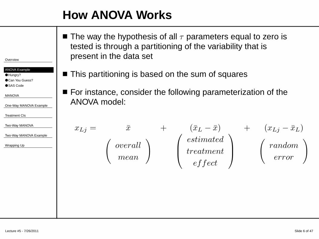
■ The way the hypothesis of all τ parameters equal to zero istested is through a partitioning of the variability that ispresent in the data set

■ This partitioning is based on the sum of squares

■ For instance, consider the following parameterization of theANOVA model:

xLj = x̄ + (x̄L − x̄) + (xLj − x̄L)(

overall

mean

)

estimated

treatment

effect

(

random

error

)

Lecture #5 - 7/26/2011 Slide 7 of 47

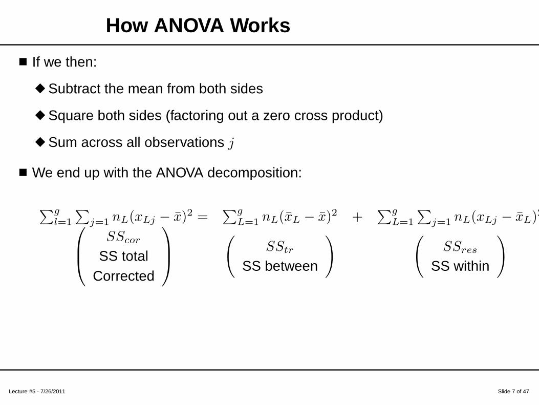
How ANOVA Works

■ If we then:

◆ Subtract the mean from both sides

◆ Square both sides (factoring out a zero cross product)

◆ Sum across all observations j

■ We end up with the ANOVA decomposition:

∑g

l=1

∑

j=1 nL(xLj − x̄)2 =∑g

L=1 nL(x̄L − x̄)2 +∑g

L=1

∑

j=1 nL(xLj − x̄L)2

SScor

SS totalCorrected

(

SStr

SS between

) (

SSres

SS within

)

Lecture #5 - 7/26/2011 Slide 8 of 47

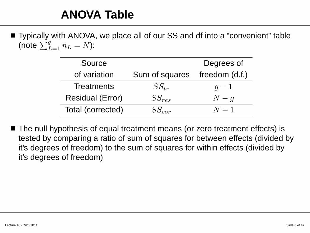
ANOVA Table

■ Typically with ANOVA, we place all of our SS and df into a “convenient” table(note

∑g

L=1 nL = N ):

Source Degrees ofof variation Sum of squares freedom (d.f.)

Treatments SStr g − 1

Residual (Error) SSres N − g

Total (corrected) SScor N − 1

■ The null hypothesis of equal treatment means (or zero treatment effects) istested by comparing a ratio of sum of squares for between effects (divided byit’s degrees of freedom) to the sum of squares for within effects (divided byit’s degrees of freedom)

Lecture #5 - 7/26/2011 Slide 9 of 47

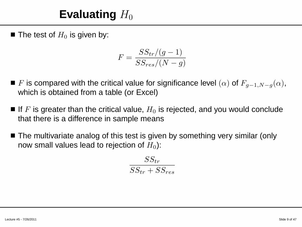
Evaluating H0

■ The test of H0 is given by:

F =SStr/(g − 1)

SSres/(N − g)

■ F is compared with the critical value for significance level (α) of Fg−1,N−g(α),which is obtained from a table (or Excel)

■ If F is greater than the critical value, H0 is rejected, and you would concludethat there is a difference in sample means

■ The multivariate analog of this test is given by something very similar (onlynow small values lead to rejection of H0):

SStr

SStr + SSres

Overview

ANOVA Example

● Hungry?

● Can You Guess?

● SAS Code

MANOVA


Treatment CIs

Two-Way MANOVA


Wrapping Up

Lecture #5 - 7/26/2011 Slide 10 of 47

Example Data SetNeter (1996, p. 676).

■ “The Kenton Food Company wished to test four differentpackage designs for a new breakfast cereal

■ “Twenty stores, with approximately equal sales volumes,were selected as the experimental units

■ “Each store was randomly assigned one of the packagedesigns, with each package design assigned to five stores

■ “The stores were chosen to be comparable in location andsales volume

■ “Other relevant conditions that could affect sales, such asprice, amount and location of shelf space, and specialpromotional efforts, were kept the same for all of the storesin the experiment”

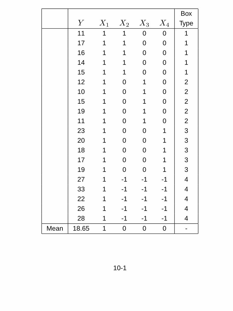
Box

Y X1 X2 X3 X4 Type

11 1 1 0 0 1

17 1 1 0 0 1

16 1 1 0 0 1

14 1 1 0 0 1

15 1 1 0 0 1

12 1 0 1 0 2

10 1 0 1 0 2

15 1 0 1 0 2

19 1 0 1 0 2

11 1 0 1 0 2

23 1 0 0 1 3

20 1 0 0 1 3

18 1 0 0 1 3

17 1 0 0 1 3

19 1 0 0 1 3

27 1 -1 -1 -1 4

33 1 -1 -1 -1 4

22 1 -1 -1 -1 4

26 1 -1 -1 -1 4

28 1 -1 -1 -1 4

Mean 18.65 1 0 0 0 -

10-1

Overview

ANOVA Example

● Hungry?

● Can You Guess?

● SAS Code

MANOVA


Treatment CIs

Two-Way MANOVA


Wrapping Up

Lecture #5 - 7/26/2011 Slide 11 of 47

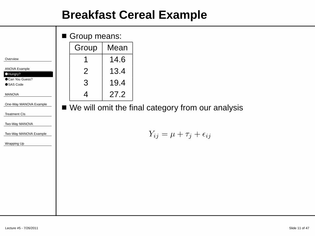
Breakfast Cereal Example

■ Group means:Group Mean

1 14.62 13.43 19.44 27.2

■ We will omit the final category from our analysis

Yij = µ + τj + ǫij

Lecture #5 - 7/26/2011 Slide 12 of 47

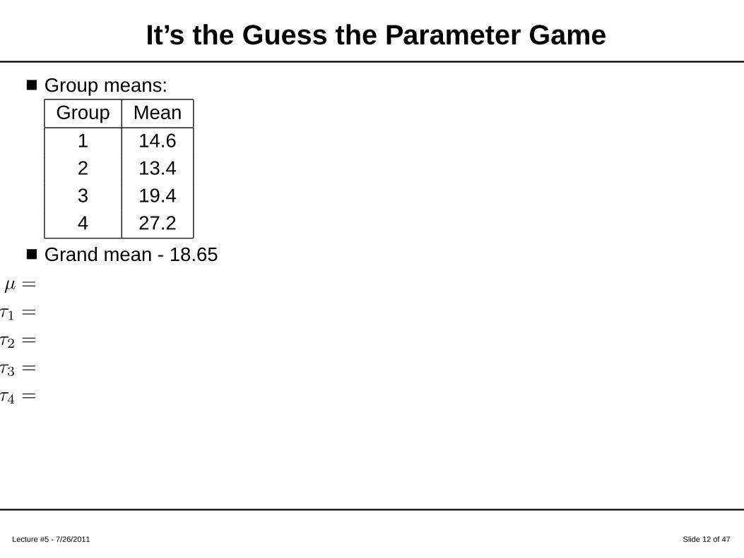
It’s the Guess the Parameter Game


1 14.62 13.43 19.44 27.2

■ Grand mean - 18.65µ =

τ1 =

τ2 =

τ3 =

τ4 =

Lecture #5 - 7/26/2011 Slide 13 of 47

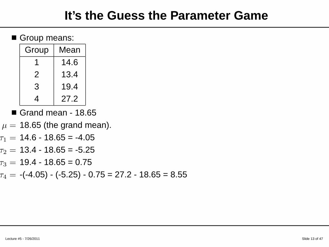
It’s the Guess the Parameter Game


1 14.62 13.43 19.44 27.2

■ Grand mean - 18.65µ = 18.65 (the grand mean).

τ1 = 14.6 - 18.65 = -4.05τ2 = 13.4 - 18.65 = -5.25τ3 = 19.4 - 18.65 = 0.75τ4 = -(-4.05) - (-5.25) - 0.75 = 27.2 - 18.65 = 8.55

Overview

ANOVA Example

● Hungry?

● Can You Guess?

● SAS Code

MANOVA


Treatment CIs

Two-Way MANOVA


Wrapping Up

Lecture #5 - 7/26/2011 Slide 14 of 47

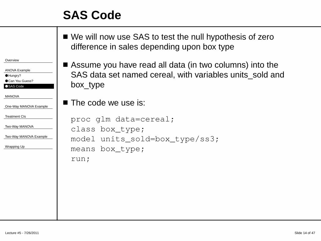
SAS Code

■ We will now use SAS to test the null hypothesis of zerodifference in sales depending upon box type

■ Assume you have read all data (in two columns) into theSAS data set named cereal, with variables units_sold andbox_type

■ The code we use is:

proc glm data=cereal;class box_type;model units_sold=box_type/ss3;means box_type;run;

Lecture #5 - 7/26/2011 Slide 15 of 47

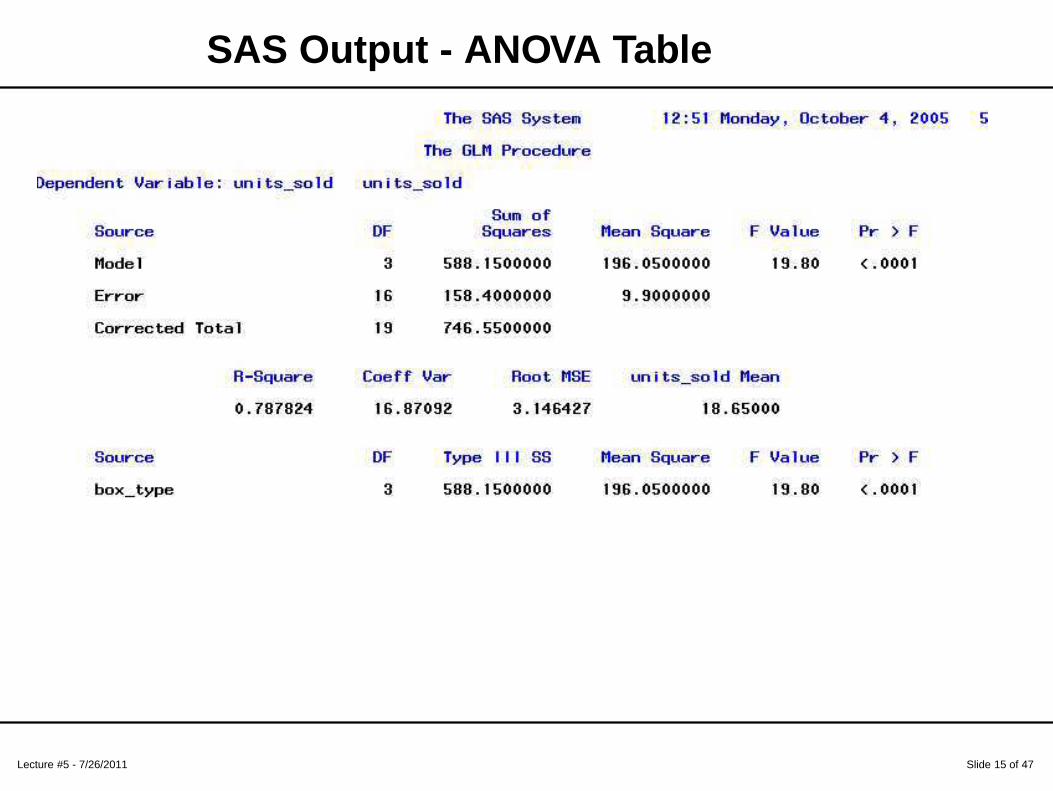
SAS Output - ANOVA Table

Lecture #5 - 7/26/2011 Slide 16 of 47

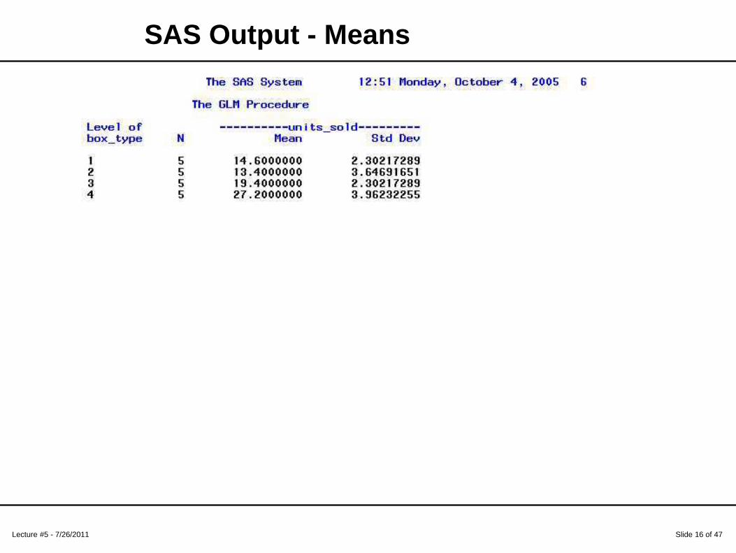
SAS Output - Means

Overview

ANOVA Example

MANOVA


Treatment CIs

Two-Way MANOVA


Wrapping Up

Lecture #5 - 7/26/2011 Slide 17 of 47

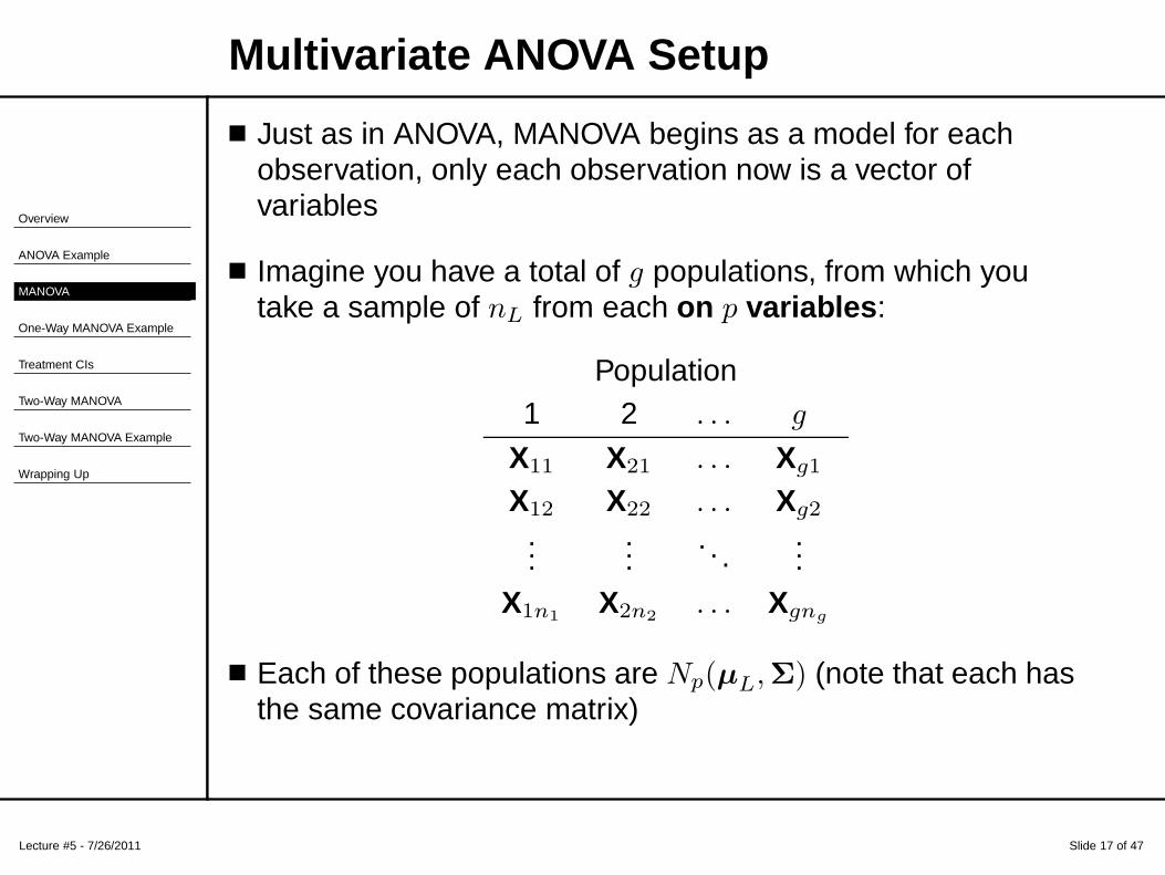
Multivariate ANOVA Setup

■ Just as in ANOVA, MANOVA begins as a model for eachobservation, only each observation now is a vector ofvariables

■ Imagine you have a total of g populations, from which youtake a sample of nL from each on p variables:

Population1 2 . . . g

X11 X21 . . . Xg1

X12 X22 . . . Xg2

......

. . ....

X1n1X2n2

. . . Xgng

■ Each of these populations are Np(µL,Σ) (note that each hasthe same covariance matrix)

Overview

ANOVA Example

MANOVA


Treatment CIs

Two-Way MANOVA


Wrapping Up

Lecture #5 - 7/26/2011 Slide 18 of 47

Hypothesis Test

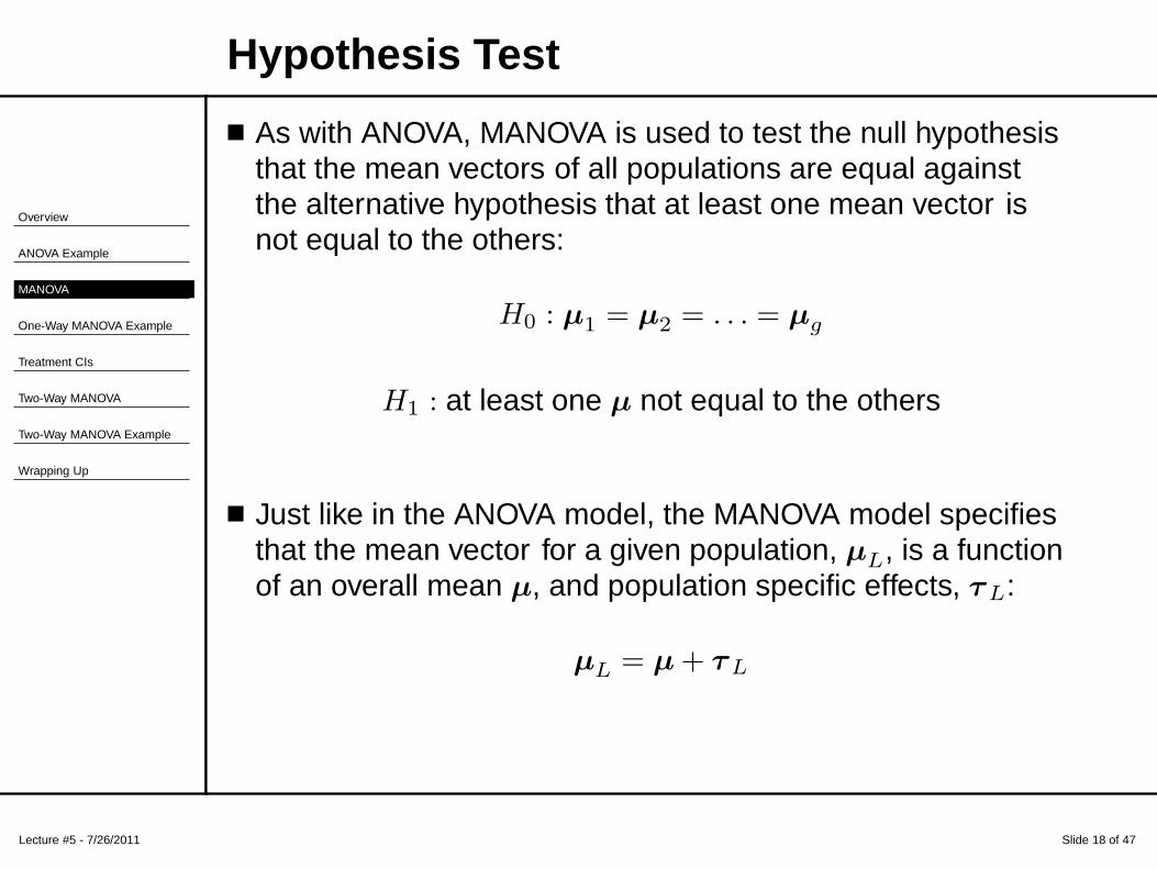
■ As with ANOVA, MANOVA is used to test the null hypothesisthat the mean vectors of all populations are equal againstthe alternative hypothesis that at least one mean vector isnot equal to the others:

H0 : µ1 = µ2 = . . . = µg

H1 : at least one µ not equal to the others

■ Just like in the ANOVA model, the MANOVA model specifiesthat the mean vector for a given population, µL, is a functionof an overall mean µ, and population specific effects, τL:

µL = µ + τL

Overview

ANOVA Example

MANOVA


Treatment CIs

Two-Way MANOVA


Wrapping Up

Lecture #5 - 7/26/2011 Slide 19 of 47

Parameterization

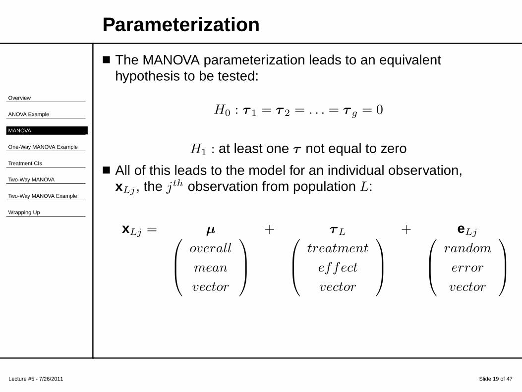
■ The MANOVA parameterization leads to an equivalenthypothesis to be tested:

H0 : τ 1 = τ 2 = . . . = τ g = 0

H1 : at least one τ not equal to zero

■ All of this leads to the model for an individual observation,xLj , the jth observation from population L:

xLj = µ + τL + eLj

overall

mean

vector

treatment

effect

vector

random

error

vector

Overview

ANOVA Example

MANOVA


Treatment CIs

Two-Way MANOVA


Wrapping Up

Lecture #5 - 7/26/2011 Slide 20 of 47

How MANOVA Works

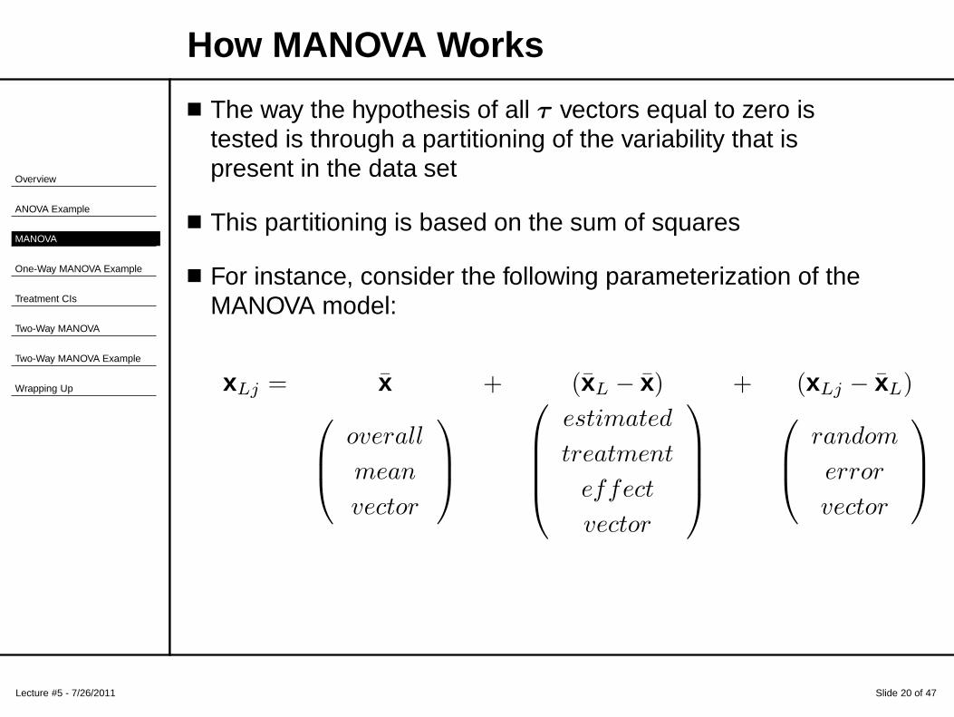
■ The way the hypothesis of all τ vectors equal to zero istested is through a partitioning of the variability that ispresent in the data set

■ This partitioning is based on the sum of squares

■ For instance, consider the following parameterization of theMANOVA model:

xLj = x̄ + (x̄L − x̄) + (xLj − x̄L)

overall

mean

vector

estimated

treatment

effect

vector

random

error

vector

Lecture #5 - 7/26/2011 Slide 21 of 47

How MANOVA Works

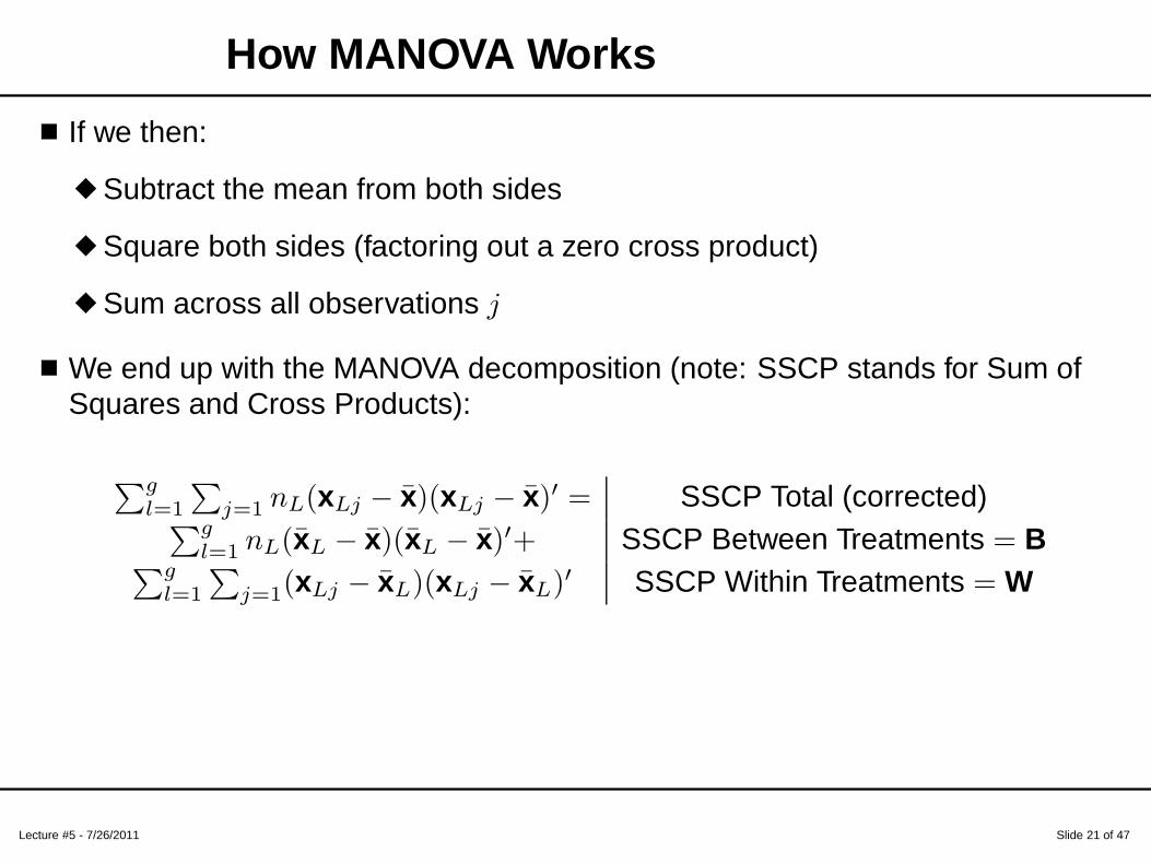
■ If we then:

◆ Subtract the mean from both sides

◆ Square both sides (factoring out a zero cross product)

◆ Sum across all observations j

■ We end up with the MANOVA decomposition (note: SSCP stands for Sum ofSquares and Cross Products):

∑g

l=1

∑

j=1 nL(xLj − x̄)(xLj − x̄)′ = SSCP Total (corrected)∑g

l=1 nL(x̄L − x̄)(x̄L − x̄)′+ SSCP Between Treatments = B∑g

l=1

∑

j=1(xLj − x̄L)(xLj − x̄L)′ SSCP Within Treatments = W

Lecture #5 - 7/26/2011 Slide 22 of 47

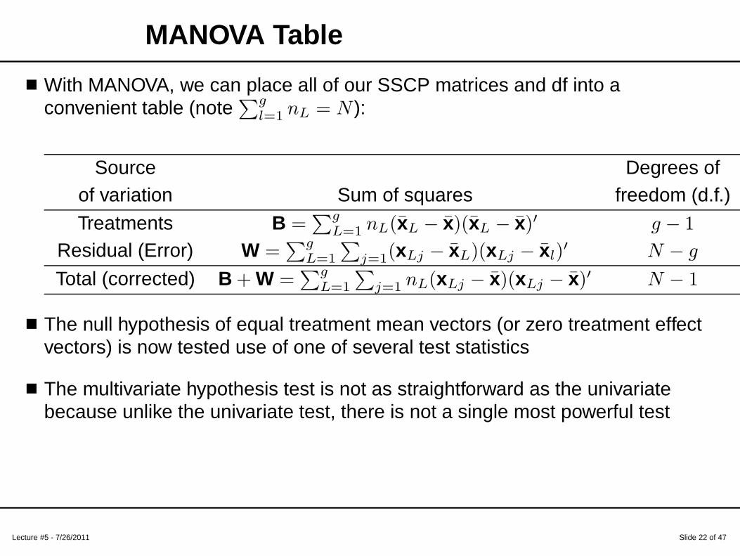
MANOVA Table

■ With MANOVA, we can place all of our SSCP matrices and df into aconvenient table (note

∑g

l=1 nL = N ):


Treatments B =∑g

L=1 nL(x̄L − x̄)(x̄L − x̄)′ g − 1

Residual (Error) W =∑g

L=1

∑

j=1(xLj − x̄L)(xLj − x̄l)′ N − g

Total (corrected) B + W =∑g

L=1

∑

j=1 nL(xLj − x̄)(xLj − x̄)′ N − 1

■ The null hypothesis of equal treatment mean vectors (or zero treatment effectvectors) is now tested use of one of several test statistics

■ The multivariate hypothesis test is not as straightforward as the univariatebecause unlike the univariate test, there is not a single most powerful test

Lecture #5 - 7/26/2011 Slide 23 of 47

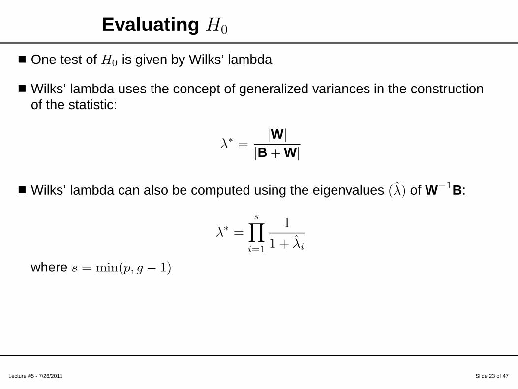
Evaluating H0

■ One test of H0 is given by Wilks’ lambda

■ Wilks’ lambda uses the concept of generalized variances in the constructionof the statistic:

λ∗ =|W|

|B + W|

■ Wilks’ lambda can also be computed using the eigenvalues (λ̂) of W−1B:

λ∗ =

s∏

i=1

1

1 + λ̂i

where s = min(p, g − 1)

Lecture #5 - 7/26/2011 Slide 24 of 47

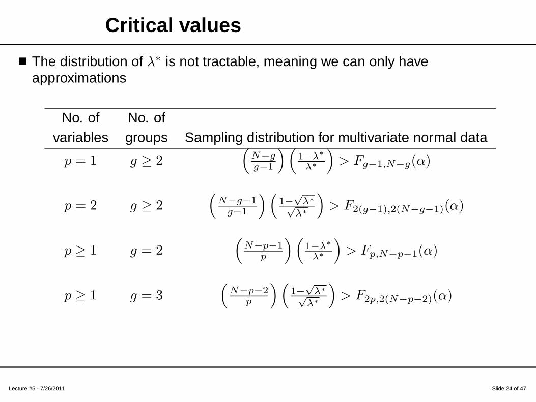
Critical values

■ The distribution of λ∗ is not tractable, meaning we can only haveapproximations

No. of No. ofvariables groups Sampling distribution for multivariate normal data

p = 1 g ≥ 2(

N−g

g−1

)(

1−λ∗

λ∗

)

> Fg−1,N−g(α)

p = 2 g ≥ 2(

N−g−1g−1

)(

1−√

λ∗

√λ∗

)

> F2(g−1),2(N−g−1)(α)

p ≥ 1 g = 2(

N−p−1p

)(

1−λ∗

λ∗

)

> Fp,N−p−1(α)

p ≥ 1 g = 3(

N−p−2p

)(

1−√

λ∗

√λ∗

)

> F2p,2(N−p−2)(α)

Overview

ANOVA Example

MANOVA


Treatment CIs

Two-Way MANOVA


Wrapping Up

Lecture #5 - 7/26/2011 Slide 25 of 47

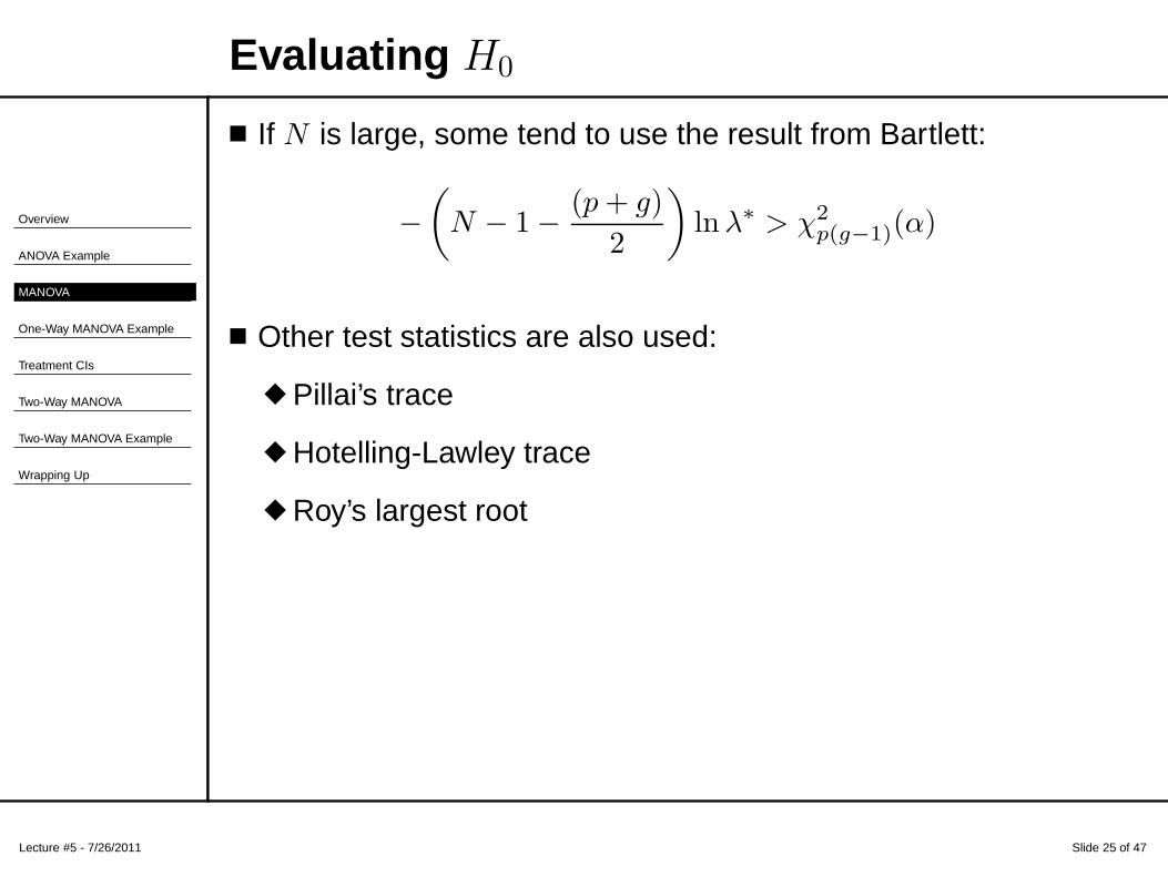
Evaluating H0

■ If N is large, some tend to use the result from Bartlett:

−

(

N − 1 −(p + g)

2

)

ln λ∗ > χ2p(g−1)(α)

■ Other test statistics are also used:

◆ Pillai’s trace

◆ Hotelling-Lawley trace

◆ Roy’s largest root

Overview

ANOVA Example

MANOVA


● SAS Code

Treatment CIs

Two-Way MANOVA


Wrapping Up

Lecture #5 - 7/26/2011 Slide 26 of 47

Motivation

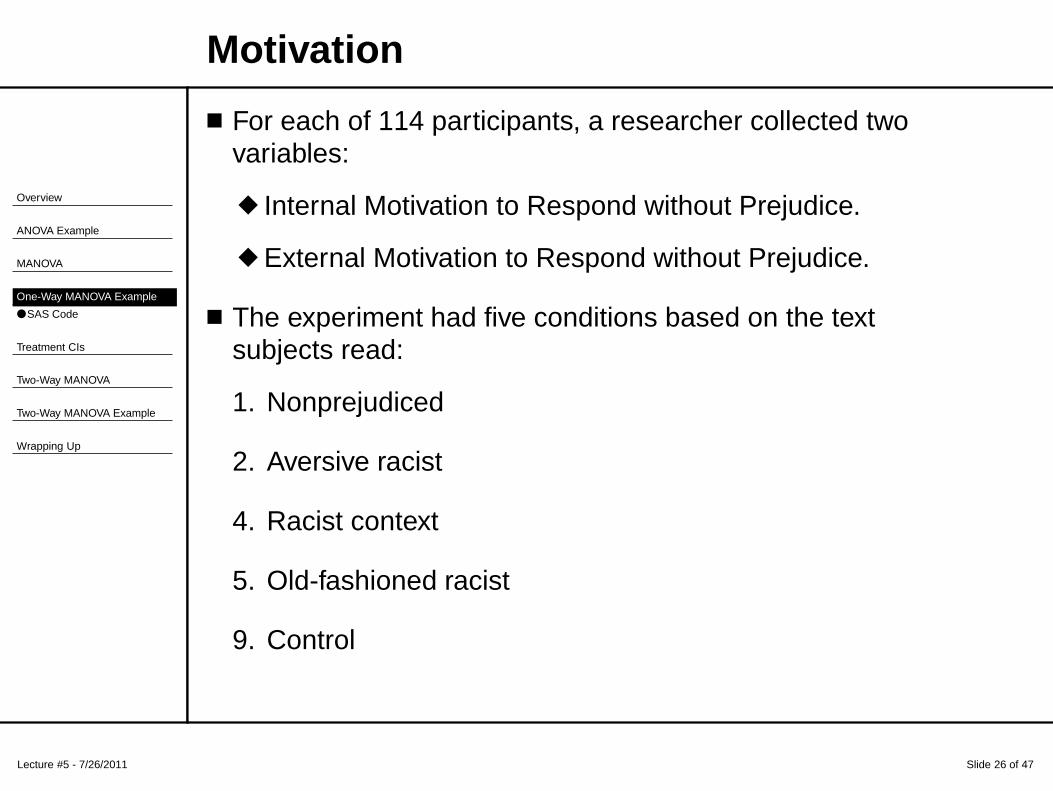
■ For each of 114 participants, a researcher collected twovariables:

◆ Internal Motivation to Respond without Prejudice.

◆ External Motivation to Respond without Prejudice.

■ The experiment had five conditions based on the textsubjects read:

1. Nonprejudiced

2. Aversive racist

4. Racist context

5. Old-fashioned racist

9. Control

Overview

ANOVA Example

MANOVA


● SAS Code

Treatment CIs

Two-Way MANOVA


Wrapping Up

Lecture #5 - 7/26/2011 Slide 27 of 47

SAS Code

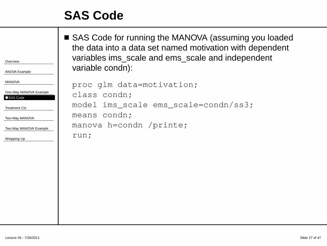
■ SAS Code for running the MANOVA (assuming you loadedthe data into a data set named motivation with dependentvariables ims_scale and ems_scale and independentvariable condn):

proc glm data=motivation;class condn;model ims_scale ems_scale=condn/ss3;means condn;manova h=condn /printe;run;

Lecture #5 - 7/26/2011 Slide 28 of 47

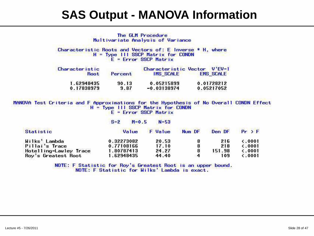
SAS Output - MANOVA Information

Lecture #5 - 7/26/2011 Slide 29 of 47

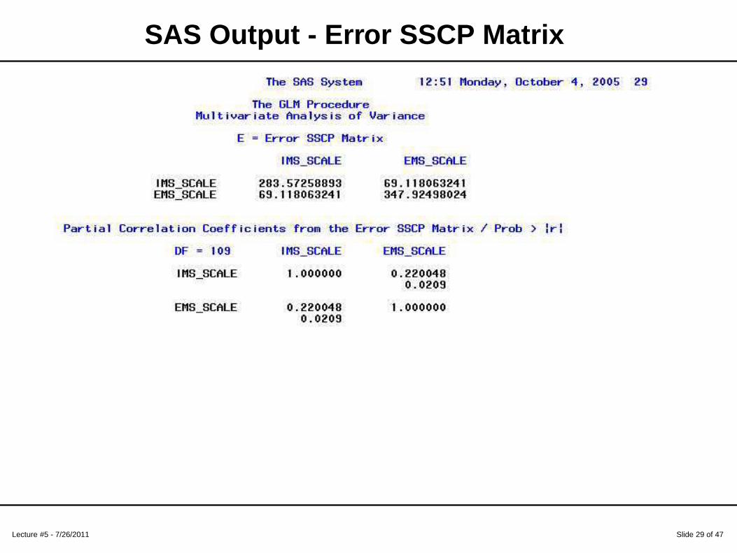
SAS Output - Error SSCP Matrix

Lecture #5 - 7/26/2011 Slide 30 of 47

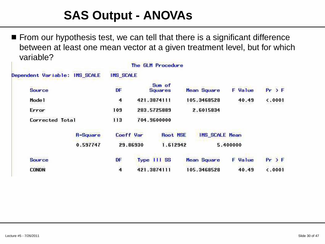
SAS Output - ANOVAs

■ From our hypothesis test, we can tell that there is a significant differencebetween at least one mean vector at a given treatment level, but for whichvariable?

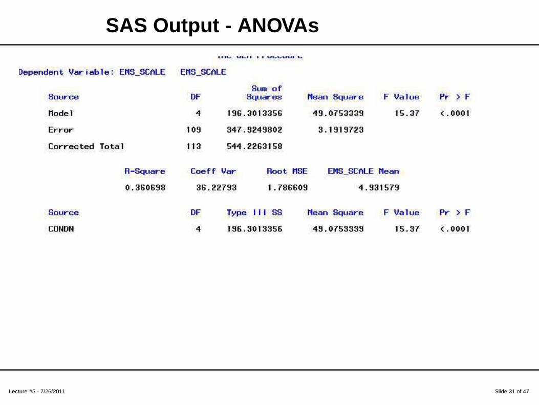
Lecture #5 - 7/26/2011 Slide 31 of 47

SAS Output - ANOVAs

Lecture #5 - 7/26/2011 Slide 32 of 47

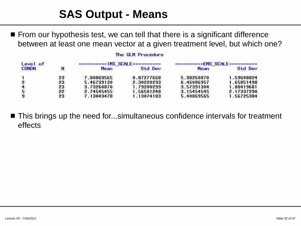
SAS Output - Means

■ From our hypothesis test, we can tell that there is a significant differencebetween at least one mean vector at a given treatment level, but which one?

■ This brings up the need for...simultaneous confidence intervals for treatmenteffects

Overview

ANOVA Example

MANOVA


Treatment CIs

● Example

Two-Way MANOVA


Wrapping Up

Lecture #5 - 7/26/2011 Slide 33 of 47

Simultaneous Treatment CIs

■ In order to further investigate the differences in means ofspecific variables at specific treatment levels, simultaneousconfidence intervals must be constructed

■ These simultaneous CIs are no different than constructingregular univariate CIs that factor in multiple measures usingthe Bonferroni method

■ The Bonferroni method ensures that the overall error rate100 × (1 − α)% is held constant for all comparisons youmight make

■ The method equates to dividing α by the number of tests thatwill be constructed

Overview

ANOVA Example

MANOVA


Treatment CIs

● Example

Two-Way MANOVA


Wrapping Up

Lecture #5 - 7/26/2011 Slide 34 of 47

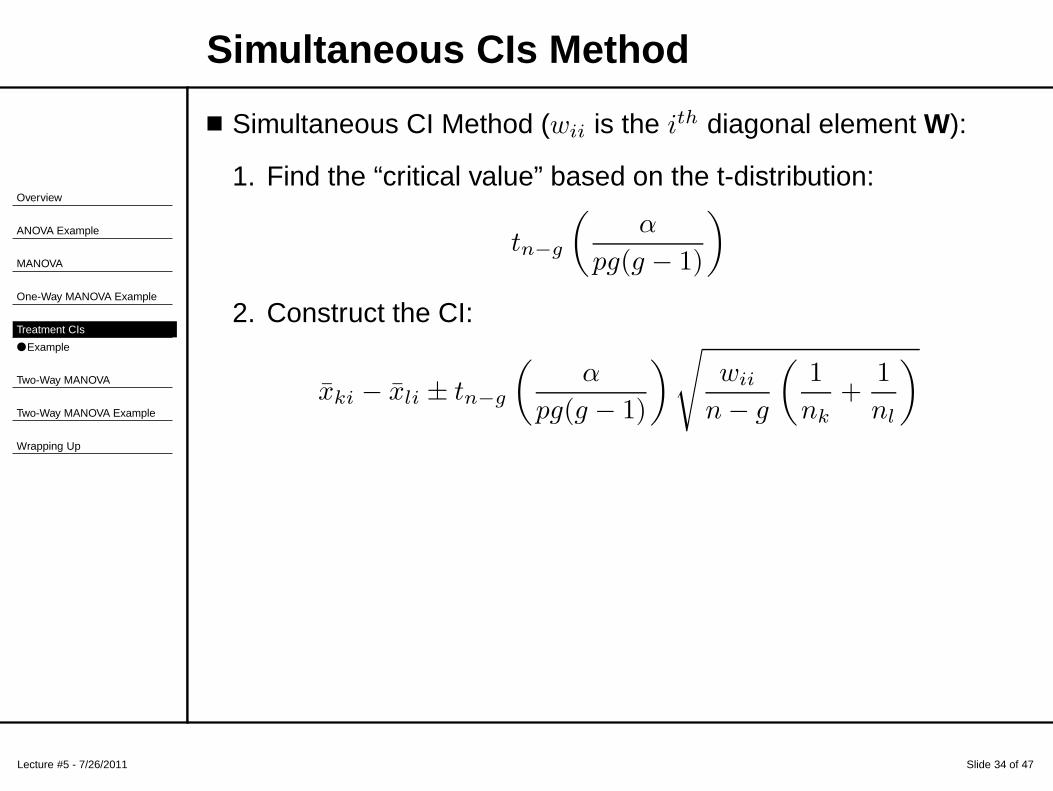
Simultaneous CIs Method

■ Simultaneous CI Method (wii is the ith diagonal element W):

1. Find the “critical value” based on the t-distribution:

tn−g

(

α

pg(g − 1)

)

2. Construct the CI:

x̄ki − x̄li ± tn−g

(

α

pg(g − 1)

)

√

wii

n − g

(

1

nk

+1

nl

)

Overview

ANOVA Example

MANOVA


Treatment CIs

● Example

Two-Way MANOVA


Wrapping Up

Lecture #5 - 7/26/2011 Slide 35 of 47

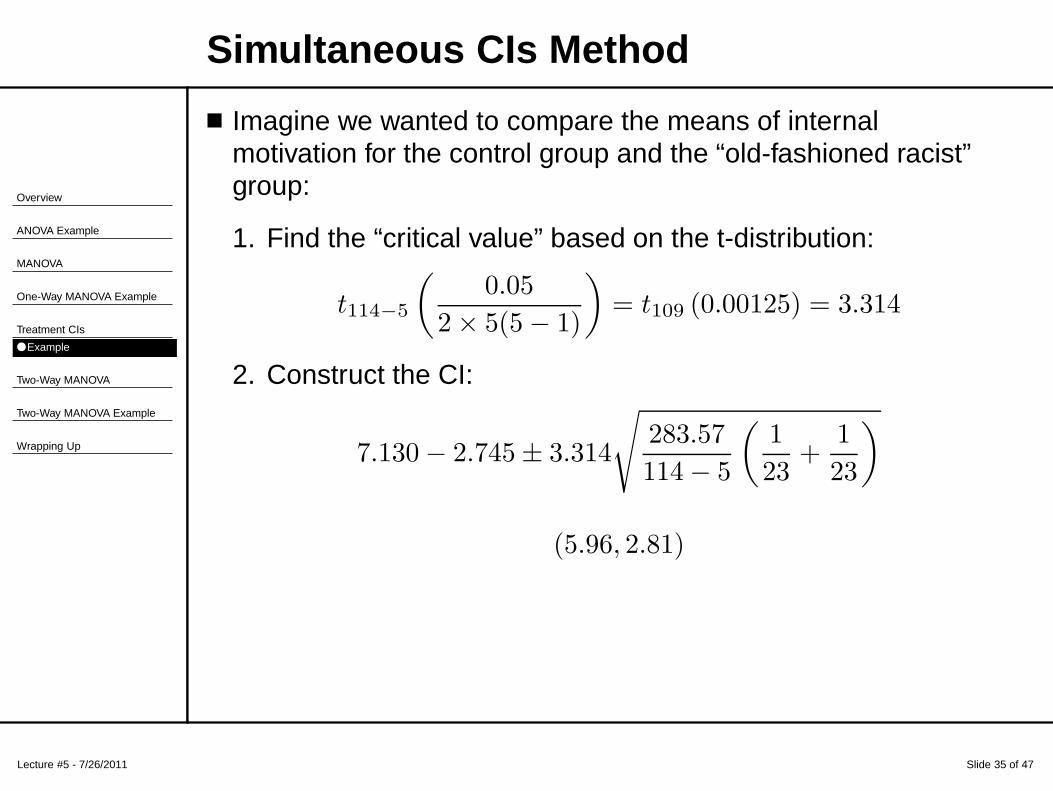
Simultaneous CIs Method

■ Imagine we wanted to compare the means of internalmotivation for the control group and the “old-fashioned racist”group:

1. Find the “critical value” based on the t-distribution:

t114−5

(

0.05

2 × 5(5 − 1)

)

= t109 (0.00125) = 3.314

2. Construct the CI:

7.130 − 2.745 ± 3.314

√

283.57

114 − 5

(

1

23+

1

23

)

(5.96, 2.81)

Overview

ANOVA Example

MANOVA


Treatment CIs

Two-Way MANOVA


Wrapping Up

Lecture #5 - 7/26/2011 Slide 36 of 47

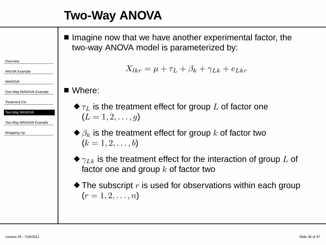
Two-Way ANOVA

■ Imagine now that we have another experimental factor, thetwo-way ANOVA model is parameterized by:

Xlkr = µ + τL + βk + γLk + eLkr

■ Where:

◆ τL is the treatment effect for group L of factor one(L = 1, 2, . . . , g)

◆ βk is the treatment effect for group k of factor two(k = 1, 2, . . . , b)

◆ γLk is the treatment effect for the interaction of group L offactor one and group k of factor two

◆ The subscript r is used for observations within each group(r = 1, 2, . . . , n)

Lecture #5 - 7/26/2011 Slide 37 of 47

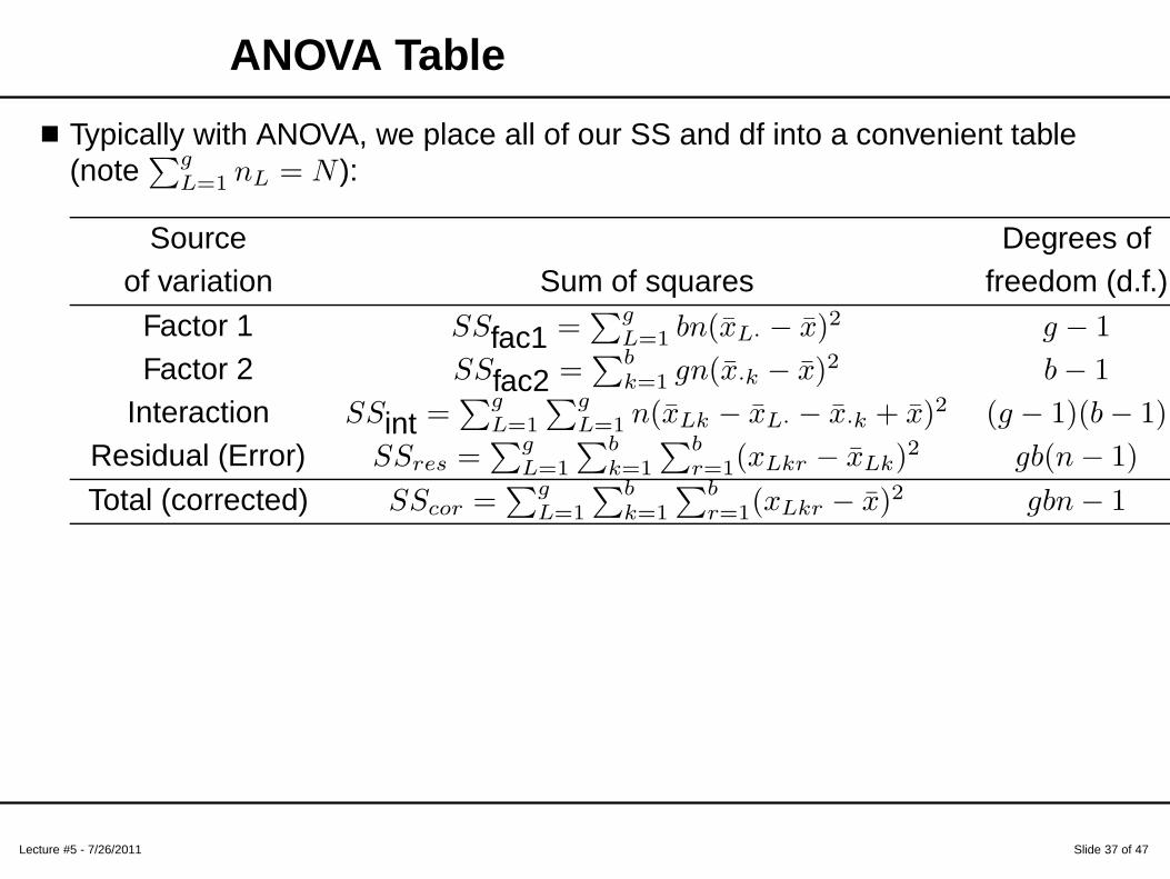
ANOVA Table

■ Typically with ANOVA, we place all of our SS and df into a convenient table(note

∑g

L=1 nL = N ):


Factor 1 SSfac1 =∑g

L=1 bn(x̄L· − x̄)2 g − 1

Factor 2 SSfac2 =∑b

k=1 gn(x̄·k − x̄)2 b − 1

Interaction SSint =∑g

L=1

∑g

L=1 n(x̄Lk − x̄L· − x̄·k + x̄)2 (g − 1)(b − 1)

Residual (Error) SSres =∑g

L=1

∑b

k=1

∑b

r=1(xLkr − x̄Lk)2 gb(n − 1)

Total (corrected) SScor =∑g

L=1

∑b

k=1

∑b

r=1(xLkr − x̄)2 gbn − 1

Overview

ANOVA Example

MANOVA


Treatment CIs

Two-Way MANOVA


Wrapping Up

Lecture #5 - 7/26/2011 Slide 38 of 47

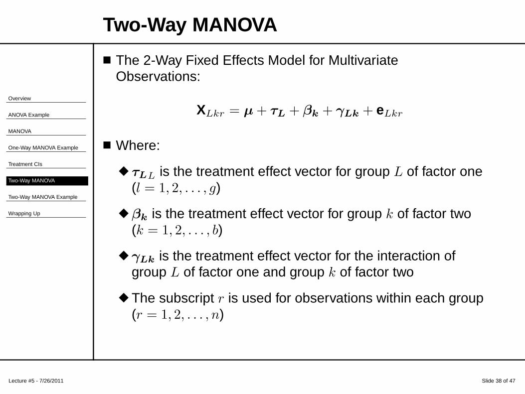
Two-Way MANOVA

■ The 2-Way Fixed Effects Model for MultivariateObservations:

XLkr = µ + τL + βk + γLk + eLkr

■ Where:

◆ τLL is the treatment effect vector for group L of factor one(l = 1, 2, . . . , g)

◆ βk is the treatment effect vector for group k of factor two(k = 1, 2, . . . , b)

◆ γLk is the treatment effect vector for the interaction ofgroup L of factor one and group k of factor two

◆ The subscript r is used for observations within each group(r = 1, 2, . . . , n)

Lecture #5 - 7/26/2011 Slide 39 of 47

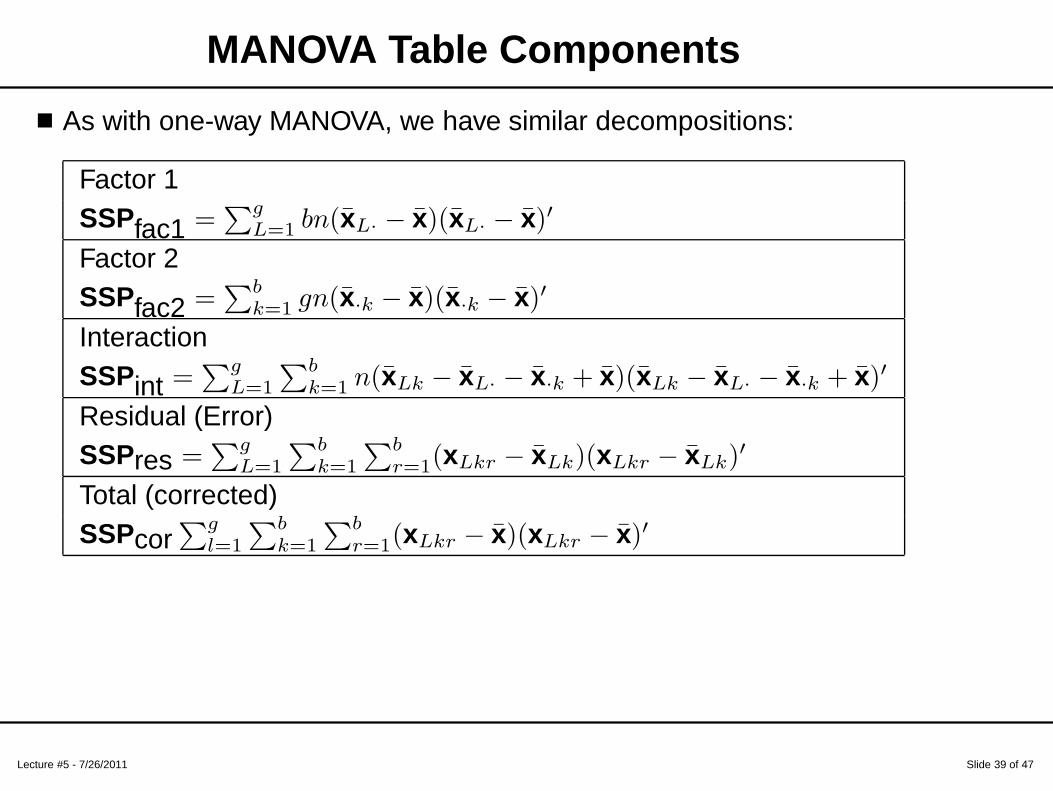
MANOVA Table Components

■ As with one-way MANOVA, we have similar decompositions:

Factor 1SSPfac1 =

∑g

L=1 bn(x̄L· − x̄)(x̄L· − x̄)′

Factor 2SSPfac2 =

∑b

k=1 gn(x̄·k − x̄)(x̄·k − x̄)′

InteractionSSPint =

∑g

L=1

∑b

k=1 n(x̄Lk − x̄L· − x̄·k + x̄)(x̄Lk − x̄L· − x̄·k + x̄)′

Residual (Error)SSPres =

∑g

L=1

∑b

k=1

∑b

r=1(xLkr − x̄Lk)(xLkr − x̄Lk)′

Total (corrected)SSPcor

∑g

l=1

∑b

k=1

∑b

r=1(xLkr − x̄)(xLkr − x̄)′

Lecture #5 - 7/26/2011 Slide 40 of 47

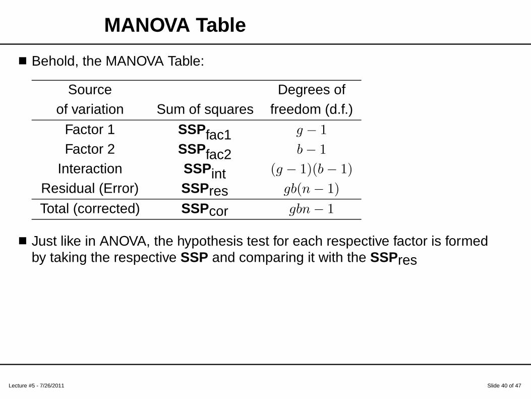
MANOVA Table

■ Behold, the MANOVA Table:


Factor 1 SSPfac1 g − 1

Factor 2 SSPfac2 b − 1

Interaction SSPint (g − 1)(b − 1)

Residual (Error) SSPres gb(n − 1)

Total (corrected) SSPcor gbn − 1

■ Just like in ANOVA, the hypothesis test for each respective factor is formedby taking the respective SSP and comparing it with the SSPres

Lecture #5 - 7/26/2011 Slide 41 of 47

Additional Designs

■ For any research design where ANOVA can be run, MANOVA can be run aswell

■ In SAS, each of these designs are implemented in the “model” and “manova”lines of the code

■ Examples of such code are found in the online SAS manual

Overview

ANOVA Example

MANOVA


Treatment CIs

Two-Way MANOVA


● Test for Interaction

● Test for Location

● Test for Variety

Wrapping Up

Lecture #5 - 7/26/2011 Slide 42 of 47

Cost data

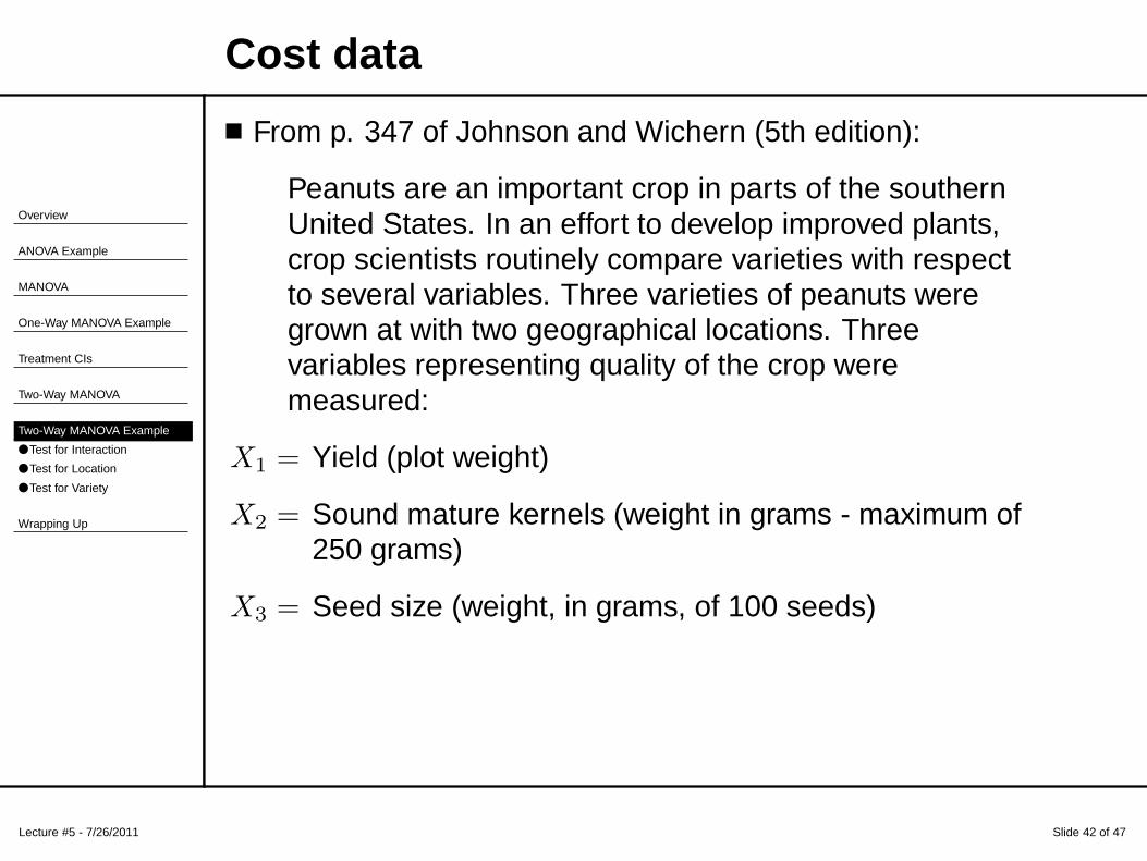
■ From p. 347 of Johnson and Wichern (5th edition):

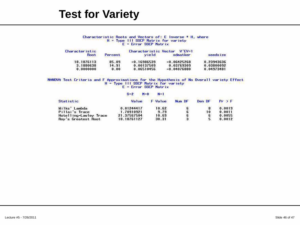
Peanuts are an important crop in parts of the southernUnited States. In an effort to develop improved plants,crop scientists routinely compare varieties with respectto several variables. Three varieties of peanuts weregrown at with two geographical locations. Threevariables representing quality of the crop weremeasured:

X1 = Yield (plot weight)

X2 = Sound mature kernels (weight in grams - maximum of250 grams)

X3 = Seed size (weight, in grams, of 100 seeds)

Lecture #5 - 7/26/2011 Slide 43 of 47

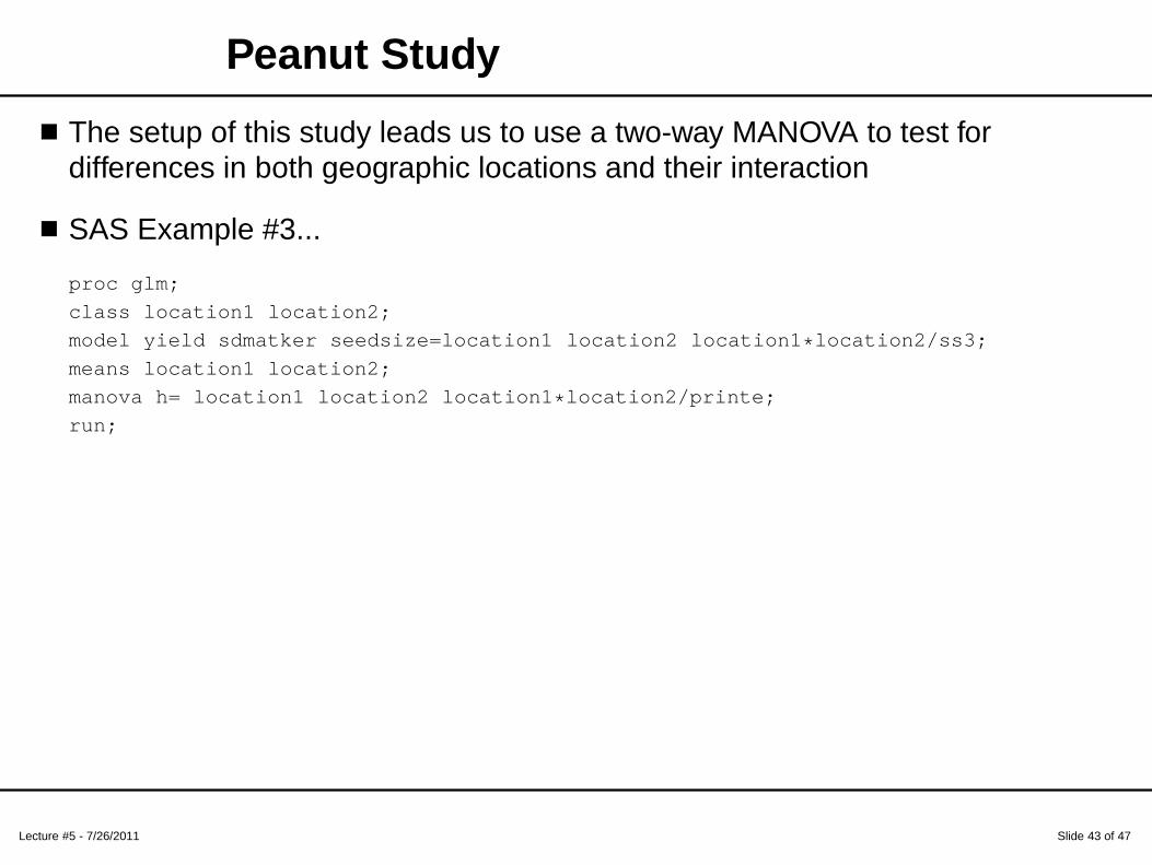
Peanut Study

■ The setup of this study leads us to use a two-way MANOVA to test fordifferences in both geographic locations and their interaction

■ SAS Example #3...

proc glm;

class location1 location2;

model yield sdmatker seedsize=location1 location2 location1*location2/ss3;

means location1 location2;

manova h= location1 location2 location1*location2/printe;

run;

Lecture #5 - 7/26/2011 Slide 44 of 47

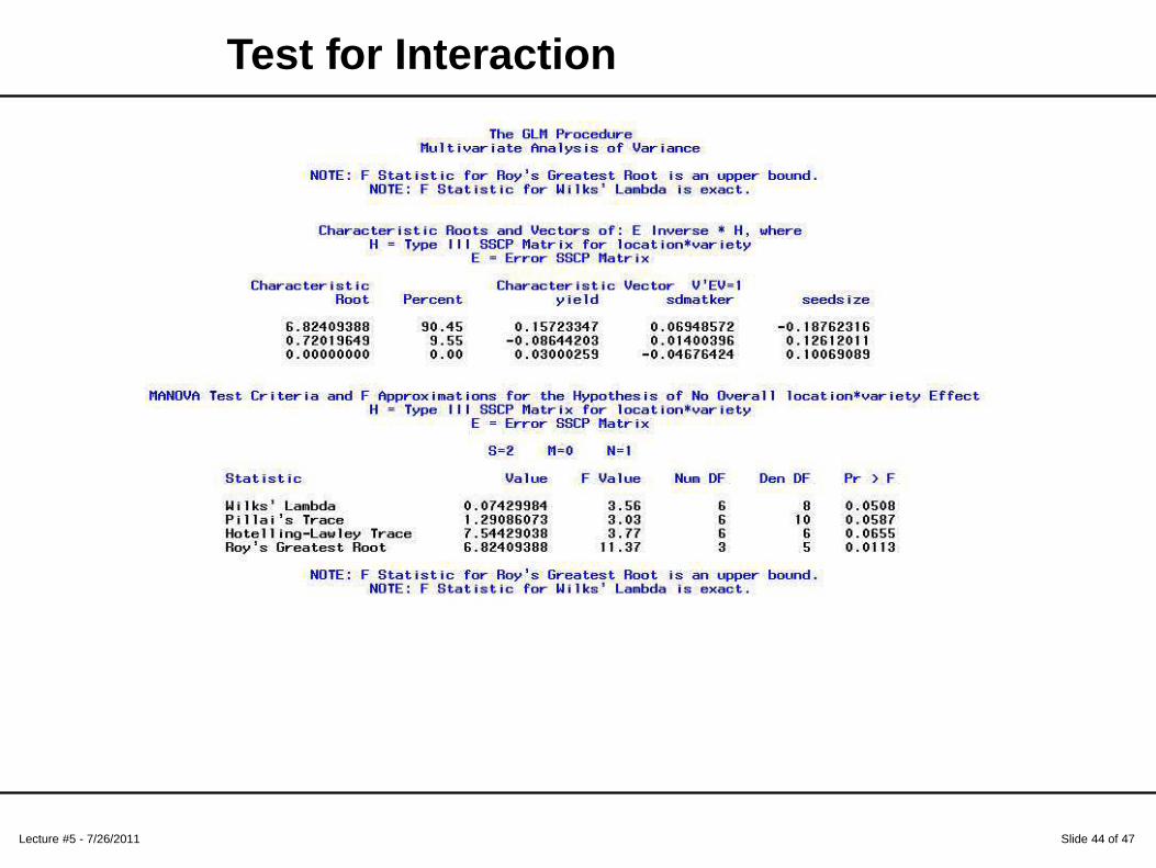
Test for Interaction

Lecture #5 - 7/26/2011 Slide 45 of 47

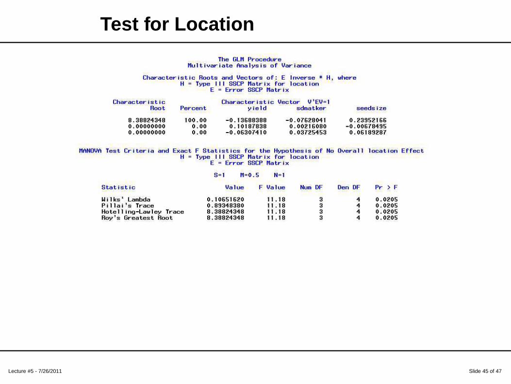
Test for Location

Lecture #5 - 7/26/2011 Slide 46 of 47

Test for Variety

Overview

ANOVA Example

MANOVA


Treatment CIs

Two-Way MANOVA


Wrapping Up

● Final Thought

Lecture #5 - 7/26/2011 Slide 47 of 47

Final Thought

■ MANOVA is a straightforward extension of univariate ANOVAmodels for hypothesis testing

■ Fixed effects MANOVA can be extended to any possibleresearch design that can be analyzed by an ANOVA

■ MANOVA is good for: times when you wish to test multiplevariables simultaneously

■ MANOVA is not good for: repeated measures with timevarying covariates (try multilevel...)

■ Next time: Discriminant analysis