


Languages
Pages
Legal


Multiscale Simulations for Soft Matter: Applications and New Developments
K. Kremer Max Planck Institute for Polymer Research, Mainz
Cambridge December, 03, 2015
COWORKERS: Debashish Mukherji, MPIP Aoife Fogarty, MPIP Luigi Delle Site, FU Berlin Matej Praprotnik , Ljubljana Christoph Junghans , Los Alamaos Simon Poblete , FZ Jülich Han Wang, Beijing, now FU Berlin Adolfo Poma , La Sapienza Rome, Sebastian Fritsch, MPIP Raffaelo Potestio, MPIP Davide Donadio, MPIP Karsten Kreis, MPIP Ralf Everaers, ENS Lyon Pep Espanol, Madrid Rafa Delgado Buscalioni, Madrid C. Clementi group (Rice), G. Ciccotti (Rome), …
Support: MMM Initiative of the MPG, Volkswagen Foundation, DAAD, KITP(NSF), DFG, ERC …
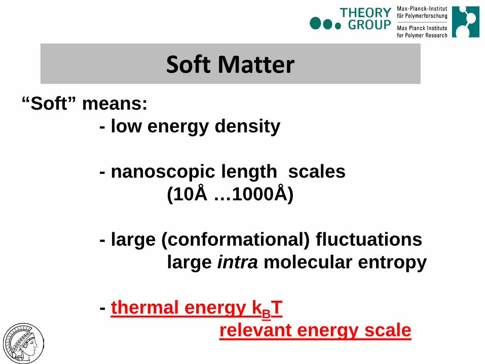
Soft Matter “Soft” means: - low energy density - nanoscopic length scales (10Å …1000Å) - large (conformational) fluctuations large intra molecular entropy - thermal energy kBT relevant energy scale
molkJkTmolkcalkT
cmkTpNnmkT
EkTeVkTJkT
KKJE
H
/5.2/6.0
2001.4
105.9105.2101.4
300/1038.1
1
4
2
21
23
⇒⇒⇒
≈⋅≈
⋅≈
⋅≈
⋅⋅=
−
−
−
−
−
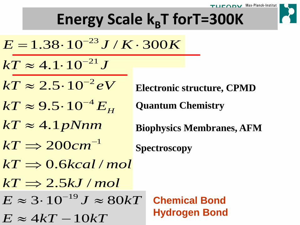
Energy Scale kBT forT=300K
Quantum Chemistry
Electronic structure, CPMD
Biophysics Membranes, AFM
Spectroscopy
kTkTEkTJE
10480103 19
−≈≈⋅≈ − Chemical Bond
Hydrogen Bond

molkJkTmolkcalkT
cmkTpNnmkT
EkTeVkTJkT
KKJE
H
/5.2/6.0
2001.4
105.9105.2101.4
300/1038.1
1
4
2
21
23
⇒⇒⇒
≈⋅≈
⋅≈
⋅≈
⋅⋅=
−
−
−
−
−
Energy Scale kBT forT=300K
Quantum Chemistry
Electronic structure, CPMD
Biophysics Membranes, AFM
Spectroscopy
kTkTEkTJE
10480103 19
−≈≈⋅≈ − Chemical Bond
Hydrogen Bond

Soft Matter – Nanostructured Matter
Volume V= L3 A: Surface and Interface Area
Nanoscopically Structured Material: V/A << 1μm => Distinction Bulk vs Surface/Interface not useful
Definition of A usually depends on the question studied!

Time
Atomistic
Soft fluid
Local Chemical Properties --- Scaling Behavior of Nanostructures Energy Dominance --- Entropy Dominance of Properties
Finite elements
Characteristic Time and Length Scales
Length
bilayer buckles Molecular
GROMACS www.gromacs.org NAMD www.ks.uiuc.edu/Research/namd/
Gaussian CPMD
Quantum
ESPResSo++ www.epresso-pp.mpg.de VOTCA www.votca.org LAMMPS lammps.sandia.gov/

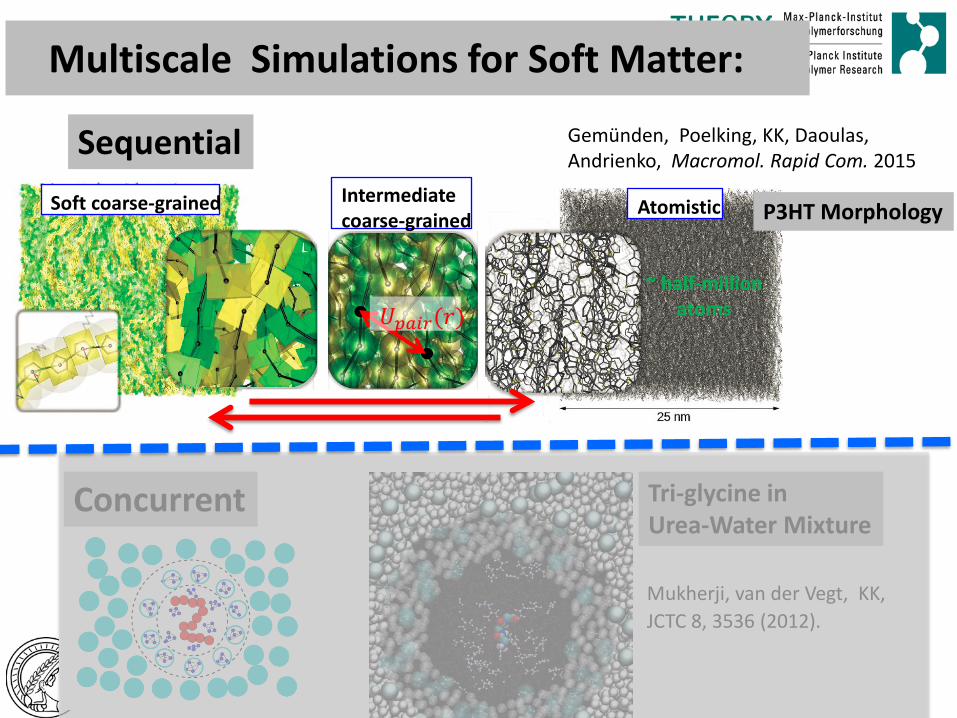
Multiscale Simulations for Soft Matter:
Sequential
Concurrent Tri-glycine in Urea-Water Mixture
Mukherji, van der Vegt, KK, JCTC 8, 3536 (2012).
Soft coarse-grained Atomistic
? 𝑈𝑈𝑝𝑝𝑝𝑝𝑝𝑝𝑝𝑝(𝑟𝑟)
Intermediate coarse-grained
Atomistic
~ half-million atoms
Gemünden, Poelking, KK, Daoulas, Andrienko, Macromol. Rapid Com. 2015
P3HT Morphology

Sequential Multiscale Simulations :
Azo Benzene LCs C. Peter, L. Delle Site, D. Marx
BPA-PC L. Delle Site, C. Abrams K. Johnston (1998ff)
Peptides C. Peter Polystyrene,
(w/wo additives) V. Harmandaris, D. Fritz N. Van der Vegt

Sequential Multiscale Simulations :
Coarse Graining (CG) micro - meso
Interplay Energy Entropy Free Energy Scale: kBT
atomistic model cg model Different general strategies to match : Structure (Mainz group, Lyubartsev…) Force (Ercolessi&Adams, Voth&Noid…) Relative Entropy (Shell, talk at this meeting) Potentials/Free Energies (e.g. Martini force field, Marrink) Methods to calculate CG interactions: (Iterative) Boltzmann Inversion Inverse MC, Iterative Force Matching Relative Entropy… (perspective W. Noid JCP 2013)
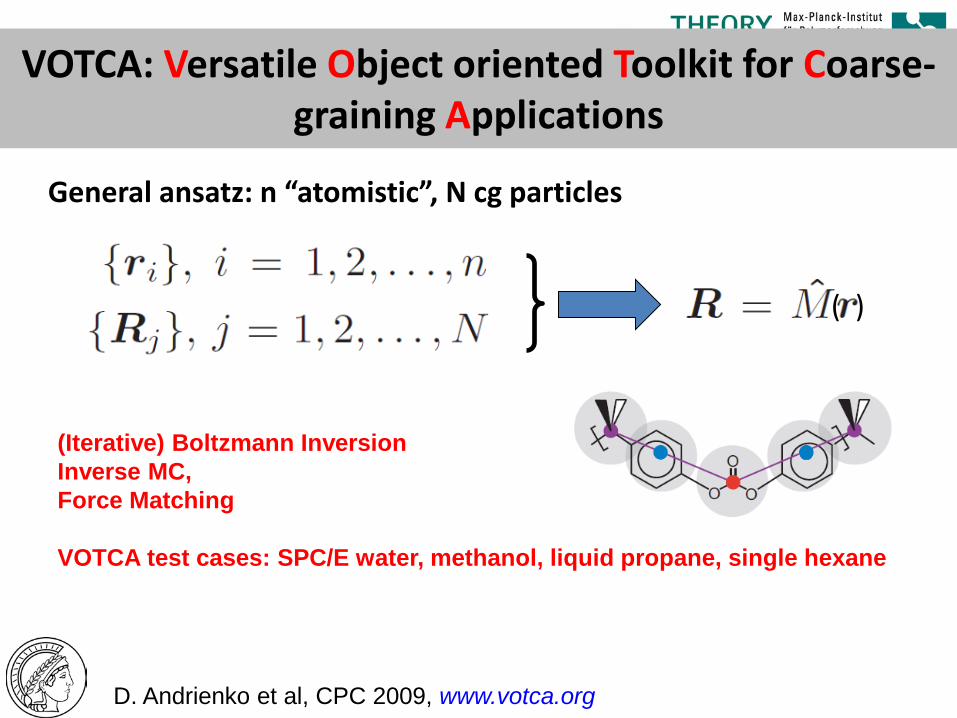
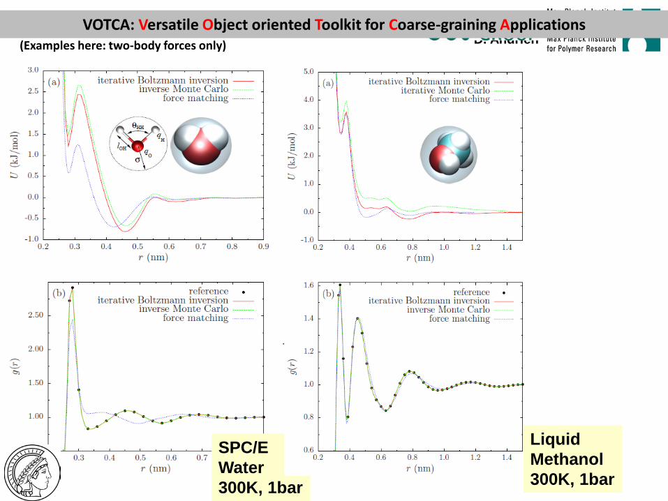
VOTCA: Versatile Object oriented Toolkit for Coarse-graining Applications
General ansatz: n “atomistic”, N cg particles
D. Andrienko et al, CPC 2009, www.votca.org
(Iterative) Boltzmann Inversion Inverse MC, Force Matching VOTCA test cases: SPC/E water, methanol, liquid propane, single hexane
( )

• Boltzmann inversion (example: bonded interactions)
Hendersen Theorem: unique correspondence between U(r) and g(r) Potential is state point dependent
Basic standard methods

Basic standard methods
• Iterative Boltzmann inversion
U(1)(r) = - kBT ln P(1)(r)

Basic standard methods
• Inverse Monte Carlo (Lyubartsev)
Similar concept as Boltzmann inversion, however sampling directly on the discretized potential u(r,…) Automatically includes correlations (unlike factorization ansatz for Boltzmann inversion) Numerically more demanding
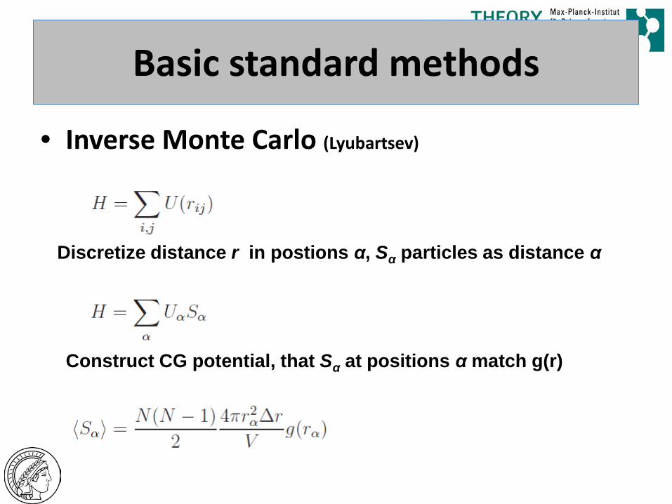
• Inverse Monte Carlo (Lyubartsev)
Discretize distance r in postions α, Sα particles as distance α
Construct CG potential, that Sα at positions α match g(r)
Basic standard methods
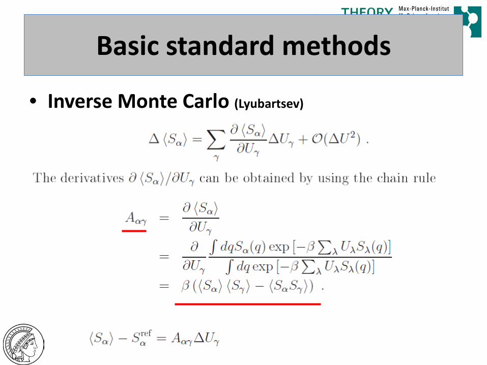
• Inverse Monte Carlo (Lyubartsev)
Basic standard methods

• Force Matching (Ercolessi&Adams, Noid&Voth et al JCP 2008ff)
ωα parameters to locate CG bead Take L snapshots, determine coefficients for N cg particles
No direct link to underlying configurations, free energy match (up to self energy of the cg particles)
Basic standard methods
D. Andrienko et al, 2009
SPC/E Water 300K, 1bar
Liquid Methanol 300K, 1bar
VOTCA: Versatile Object oriented Toolkit for Coarse-graining Applications (Examples here: two-body forces only)
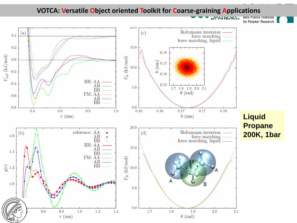
D. Andrienko et al, 2009
Liquid Propane 200K, 1bar
VOTCA: Versatile Object oriented Toolkit for Coarse-graining Applications

• Iterative Boltzmann inversion direct, needs further refining “afterwards”
• Inverse Monte Carlo more precise than IBI, includes higher order correlations, more demanding, slow convergence
• Force Matching no close link to underlying configurations, approximative solutions, needs three…body interactions, based on matching thermodynamic properties
• “other Methods” often mixed approaches for inter and intra molecular properties, other method “restricted entropy” approach (M. Scott Shell)
Comparison particle based methods
Representability and Transferability Issues
Interplay Energy Entropy Free Energy Scale: kBT
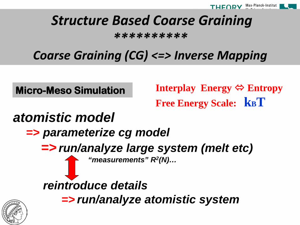
Micro-Meso Simulation
atomistic model => parameterize cg model => run/analyze large system (melt etc) “measurements” R2(N)… reintroduce details => run/analyze atomistic system
Structure Based Coarse Graining **********
Coarse Graining (CG) <=> Inverse Mapping

Coarse-graining: map bead-spring chain over molecular structure. => Many fewer degrees of freedom
Inverse mapping: grow atomic structure on top of coarse- grained backbone =>Large length-scale equilibration in an atomically resolved polymer
Structure Based Molecular Coarse-Graining: Bisphenol-A-Polycarbonate
9.3-11.5 Å
W. Tschöp, K. Kremer, J. Batoulis, T. Bürger, O. Hahn Acta Polym. 49, 61 (1998); ibid. 49, 75, ff
Speedup ≈ 104 !

Interaction Energies in the Coarse-Grained Model
• Excluded volume • Bonds • Angles • Torsions
U
P
Angle potentials are T-dependent Boltzmann inversions; e.g., at carbonate:
T = 570 K

⇐⇐⇐⇐
Coarse grained BPA-PC chain
All atom model
How good are generated conformation? Inverse Mapping:
Reintroduce Chemical Details

Structure factors of BPA-PC melt
Comparison: Simulation vs n-Scattering
22
A37)( o
G
NNR
≅
Well equilibrated coarse grained AND all atom melt configurations!
J. Eilhard et al, J. Chem. Phys. 110, 1819 (1999) B. Hess et al, Soft Matter 2006

PC at Ni Surface: Role of Chain Ends Energy - Entropy Competition
Energy Entropy
L. Delle Site et al., J.Am.Chem.Soc.; 126; 2004; 2944

Generalization: Bottom up ↔ Top down: Soft models => particle based models
Database for many specific systems
Zhang, Stuehn, Daoulas, KK, 2014, 2015
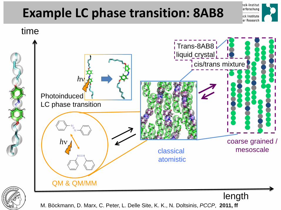
M. Böckmann, D. Marx, C. Peter, L. Delle Site, K. K., N. Doltsinis, PCCP, 2011, ff
QM & QM/MM
hν coarse grained / mesoscale classical
atomistic
hν
Trans-8AB8 liquid crystal
cis/trans mixture
Photoinduced LC phase transition
length
time
Example LC phase transition: 8AB8
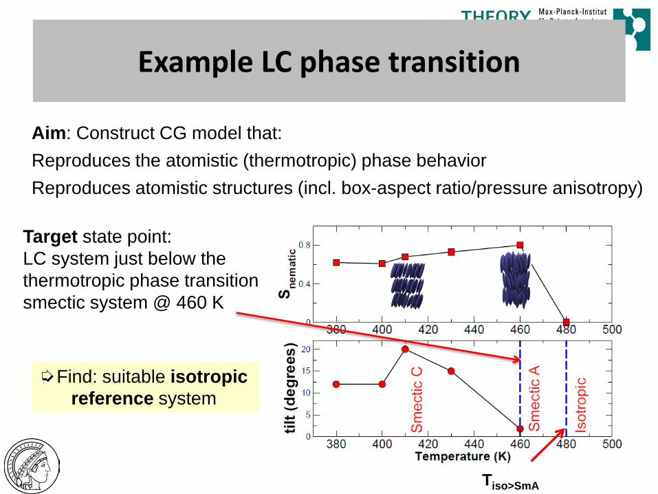
Example LC phase transition
Aim: Construct CG model that: Reproduces the atomistic (thermotropic) phase behavior Reproduces atomistic structures (incl. box-aspect ratio/pressure anisotropy)
Target state point: LC system just below the thermotropic phase transition smectic system @ 460 K
Tiso>SmA
➭Find: suitable isotropic reference system
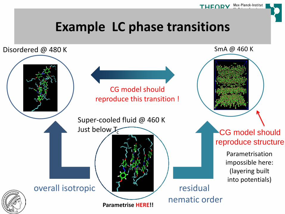
Example LC phase transitions SmA @ 460 K Disordered @ 480 K
Super-cooled fluid @ 460 K Just below Tc
CG model should reproduce this transition !
Parametrisation impossible here:
(layering built into potentials)
CG model should reproduce structure
overall isotropic residual nematic order
Parametrise HERE!!
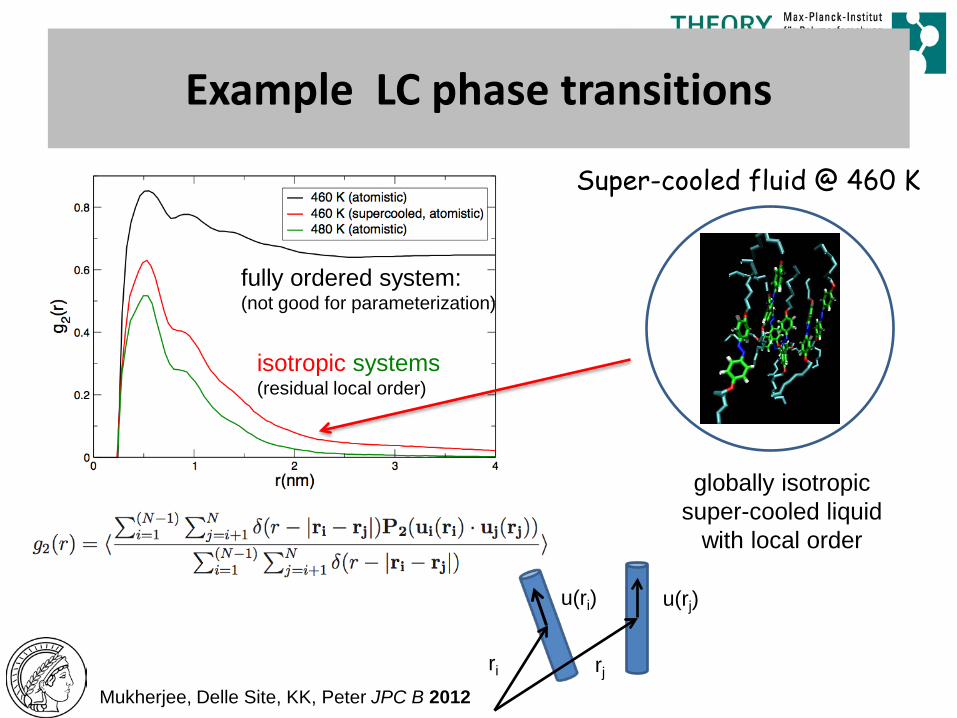
fully ordered system: (not good for parameterization)
isotropic systems (residual local order)
ri rj
u(ri) u(rj)
Example LC phase transitions
globally isotropic super-cooled liquid
with local order
Super-cooled fluid @ 460 K
Mukherjee, Delle Site, KK, Peter JPC B 2012

Example LC phase transitions
Mukherjee, Delle Site, KK, Peter JPC B 2012
➮CG model reproduces LC structure …
orde
ring
alon
g z
axis
CG model
backmapped atomistic
atomistic
atomistic
CG (new model)
backmapped atomistic
CG (old model, fragment-based)
nem
atic
ord
er p
aram
eter
MD, SCMF Processing Nonequilibrium

Sequential Multiscale Simulations :
• robust, versatile for “simple” systems (amorphous polymers, LC systems…)
• CG potentials state point dependent ⇒ transferability and representability issues of interactions (example isotropic smectic transition in 8AB8 LC systems) Length scale mapping obvious, but time scale…
• Scaling of dynamics
• Amorphous polymer melt (PS) • Smectic LC system (8AB8)
Sequential Multiscale Simulations :
• Scaling of dynamics • Amorphous polymer melt (PS)

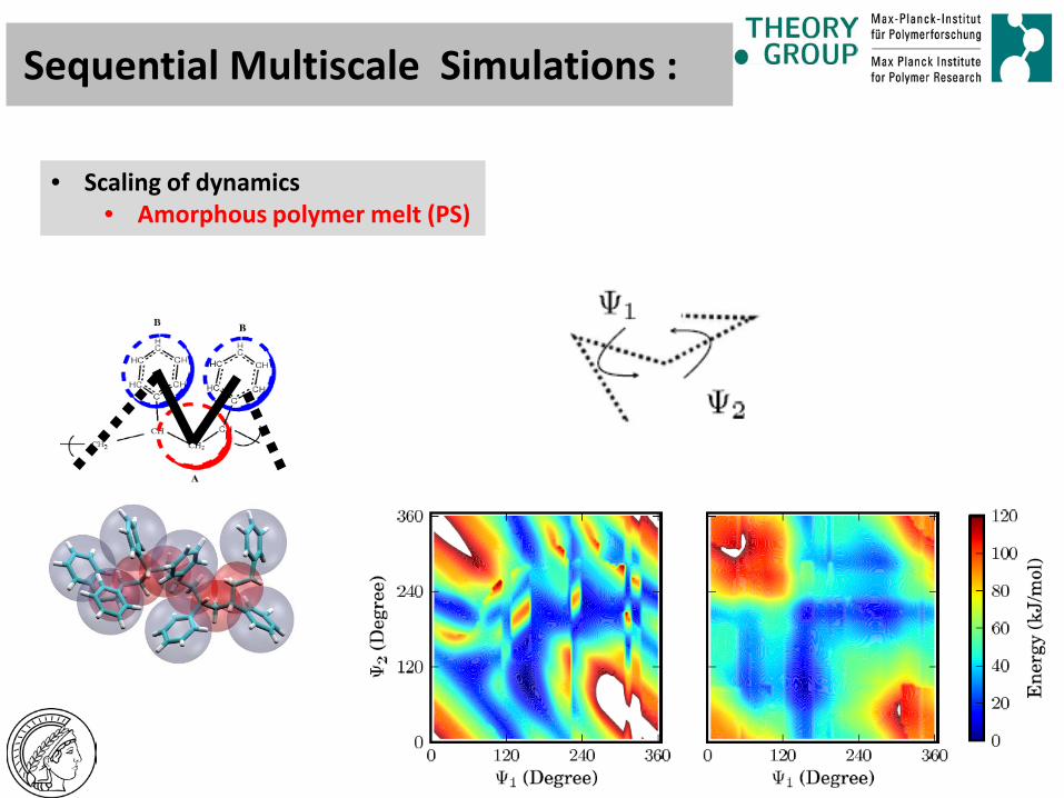
Sequential Multiscale Simulations :
• Scaling of dynamics • Amorphous polymer melt (PS)
Mapping times for short distance displacements (≈ 10 – 20 Å): 400 ps (AA sim) ↔ 1τLJ (CG sim)
Experiment: Raw FRS data, Sillescu
Simulation: NO adjustable parameter
V. Harmandaris, KK, Soft Matt. 2009
≠
dominates dynamics
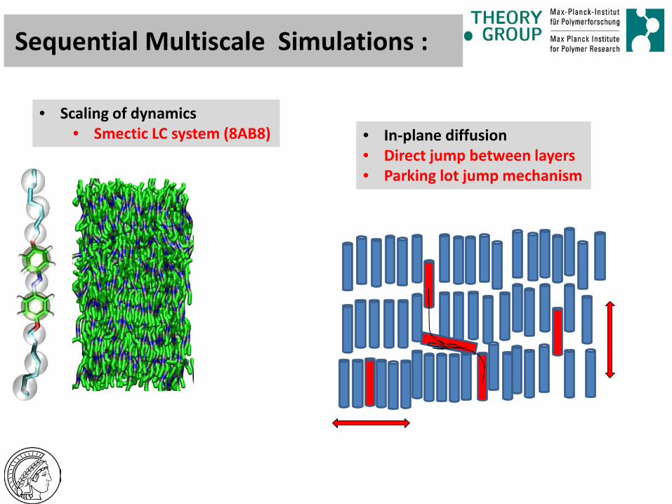
Sequential Multiscale Simulations :
• Scaling of dynamics • Smectic LC system (8AB8) • In-plane diffusion
• Direct jump between layers • Parking lot jump mechanism

Sequential Multiscale Simulations :
• Scaling of dynamics • Smectic LC system (8AB8)
• In-plane diffusion • Direct jump between layers • Parking lot jump mechanism
parking lot direct
Free energy surface CG AA
z
Cos θ

Sequential Multiscale Simulations :
• Scaling of dynamics • Smectic LC system (8AB8)
• In-plane diffusion • Direct jump between layers • Parking lot jump mechanism
Process CG Atomistic
Jump time (straight)
0.15 τ 0.2 ns
Jump time (pkl) Timestraight/ Timepkl
1.7 τ 0.088
1.0 ns ≠ 0.2
⇒ Severe problems for structure formation etc
Free energy surface CG AA
z
Cos θ
M. Deserno et al., Nature, 2007 Andrienko et al,
PRL 98, 227402 (2007) C. Peter et al, 2008ff
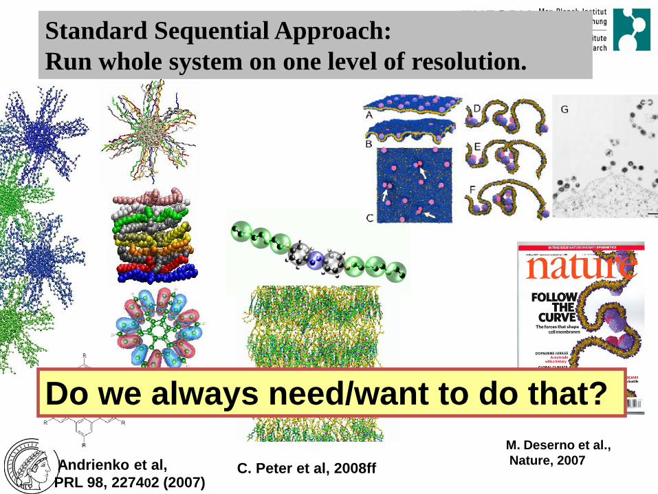
Standard Sequential Approach: Run whole system on one level of resolution.
Do we always need/want to do that?
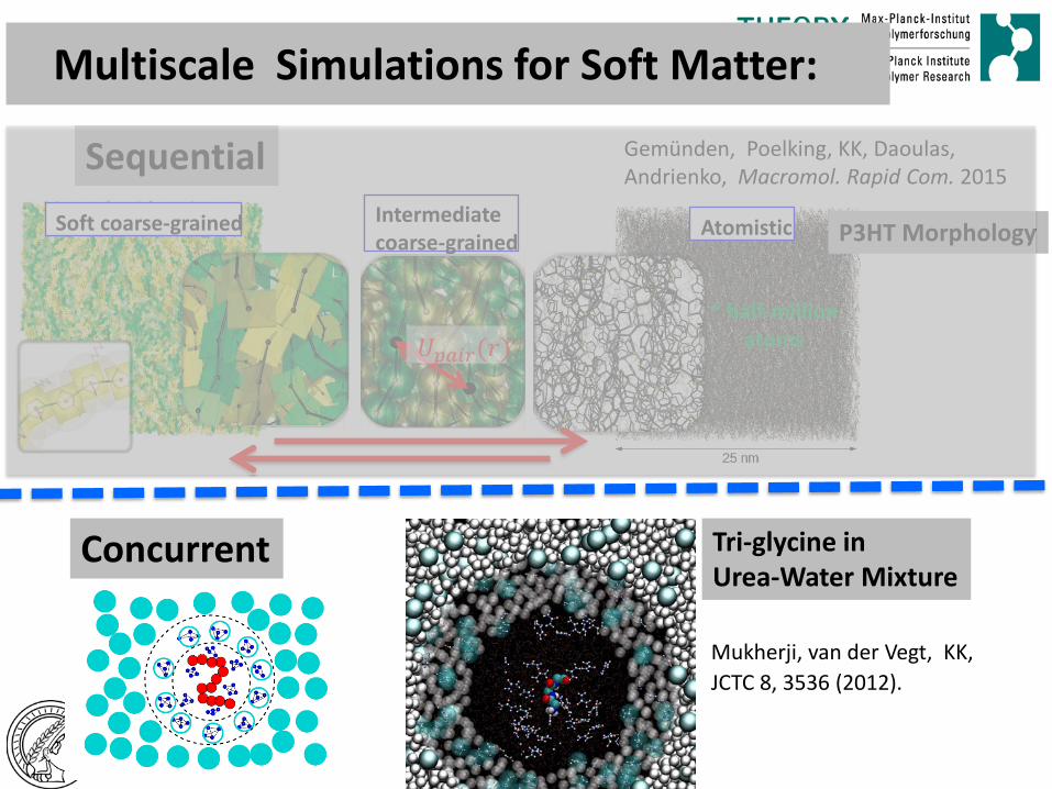
Multiscale Simulations for Soft Matter:
Sequential
Concurrent Tri-glycine in Urea-Water Mixture
Mukherji, van der Vegt, KK, JCTC 8, 3536 (2012).
Soft coarse-grained Atomistic
? 𝑈𝑈𝑝𝑝𝑝𝑝𝑝𝑝𝑝𝑝(𝑟𝑟)
Intermediate coarse-grained
Atomistic
~ half-million atoms
Gemünden, Poelking, KK, Daoulas, Andrienko, Macromol. Rapid Com. 2015
P3HT Morphology

AdResS Adaptive Resolution MD Simulation
Theory: M. Praprotnik, KK, L. Delle Site, PRE 75, 017701 (2007), JPhys A MathTh F281 (2007)
Method: Praprotnik, Delle Site, KK: J. Chem. Phys. 123, 224106 (2005) & Phys. Rev. E 73, 066701 (2006)

Requirements (for zooming in) Same mass density (?) Same temperature (?) No free energy barriers Smooth transition forces Same center-center g(r) (?)
Free exchange between regimes
(Simple two body potential)
⇒ “Some similarities” to 1st order phase transition ⇒ “Phase equilibrium”
Adaptive Methods: Changing degrees of freedom (DOFs) on the fly
VW Foundation Project M. Praprotnik, L. DelleSite, KK, JCP 2005, PRE (2006)
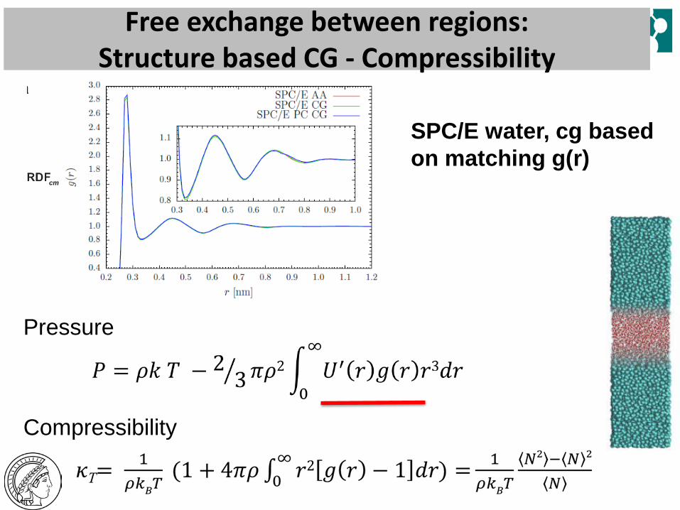
Free exchange between regions: Structure based CG - Compressibility
SPC/E water, cg based on matching g(r)
Pressure
Compressibility
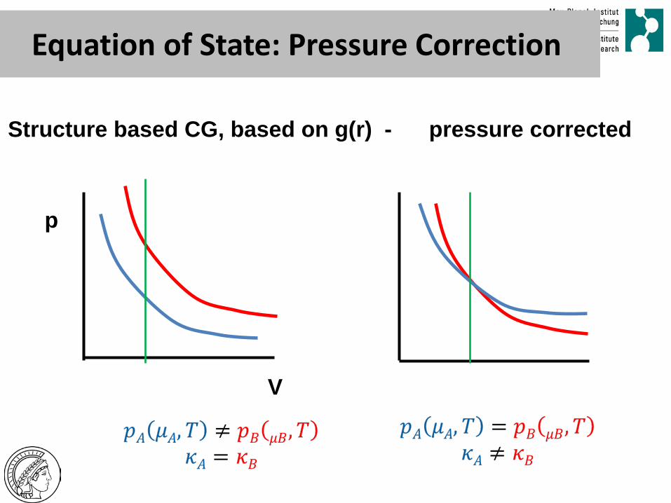
Equation of State: Pressure Correction
Structure based CG, based on g(r) - pressure corrected
p
V

Structure based CG, based on g(r) - pressure corrected
p
V
Equation of State: Pressure Correction

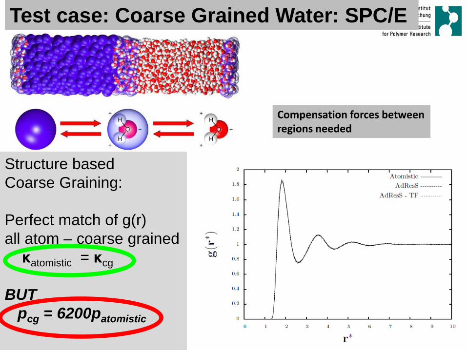
Structure based Coarse Graining: Perfect match of g(r) all atom – coarse grained κatomistic = κcg BUT pcg = 6200patomistic
Test case: Coarse Grained Water: SPC/E
Compensation forces between regions needed
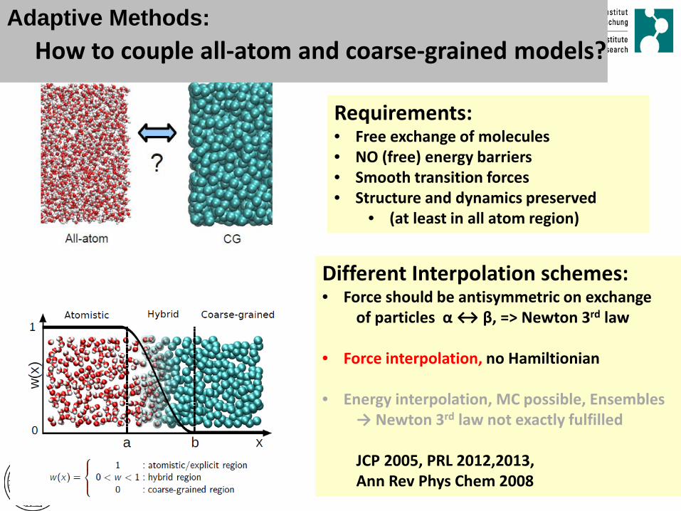
Adaptive Methods:
Requirements: • Free exchange of molecules • NO (free) energy barriers • Smooth transition forces • Structure and dynamics preserved
• (at least in all atom region)
Different Interpolation schemes: • Force should be antisymmetric on exchange of particles α ↔ β, => Newton 3rd law • Force interpolation, no Hamiltionian
• Energy interpolation, MC possible, Ensembles → Newton 3rd law not exactly fulfilled
JCP 2005, PRL 2012,2013, Ann Rev Phys Chem 2008
How to couple all-atom and coarse-grained models?
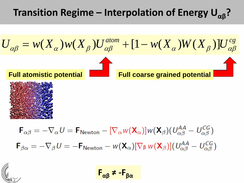
Transition Regime – Interpolation of Energy Uαβ?
cgatom UXWXwUXwXwU αββααββααβ )]()(1[)()( −+=
Full atomistic potential Full coarse grained potential
Fαβ ≠ -Fβα
β

cgatom UXWXwUXwXwU αββααββααβ )]()(1[)()( −+=
Full atomistic potential Full coarse grained potential
• Drift terms from W(x) • Violation of Newton’s 3rd law • Mathematical inconsistencies at boundaries
• There exists no W(x), such that forces become conservative (L. Delle Site PRE 2007) => Force interpolation
Transition Regime – Interpolation of Energy Uαβ?
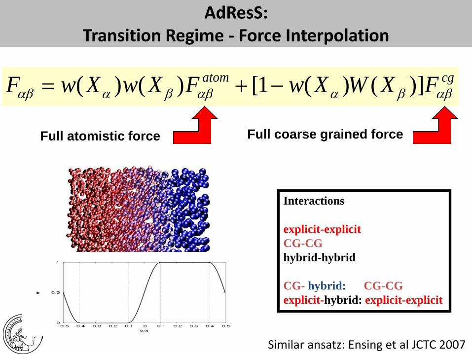
AdResS: Transition Regime - Force Interpolation
cgatom FXWXwFXwXwF αββααββααβ )]()(1[)()( −+=
Interactions explicit-explicit CG-CG hybrid-hybrid CG- hybrid: CG-CG explicit-hybrid: explicit-explicit
Full atomistic force Full coarse grained force
Similar ansatz: Ensing et al JCTC 2007

AdResS: Transition Regime - Force Interpolation
cgatom FXWXwFXwXwF αββααββααβ )]()(1[)()( −+=
Interactions explicit-explicit CG-CG hybrid-hybrid CG- hybrid: CG-CG explicit-hybrid: explicit-explicit
Full atomistic force Full coarse grained force Transition regime: Force interpolation (Newtons 3rd law fulfilled, no drift forces) No transition energy function defined! Pressure, Temperature, Density everywhere well defined Thermostat needed (no microcanonical simulation possible!)
* Similar problem already in H.C. Andersen, JCP 72, 2384 (1979)

Theoretical Basis: Temperature… Necessity of Thermostat
Special Example: Two spherical particles, same EoS and same number DOFs
=
p
V
Extensive theoretical work by L. Delle Site
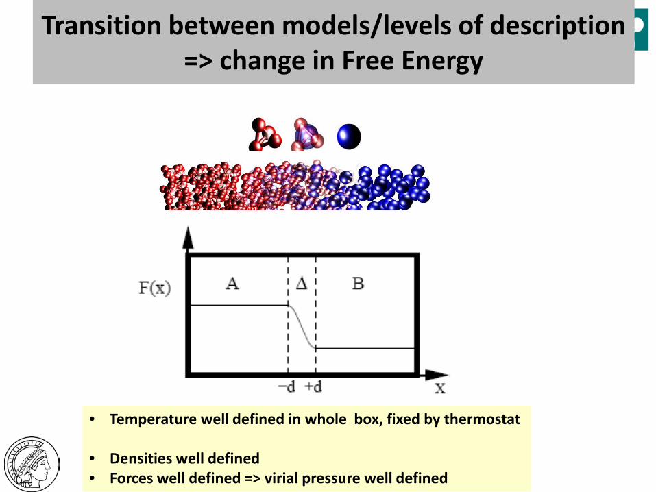
Transition between models/levels of description => change in Free Energy
• Temperature well defined in whole box, fixed by thermostat
• Densities well defined • Forces well defined => virial pressure well defined

A unified framework for Force-Based & Energy-Based Adaptive Resolution
Simulations
Additive instead of multiplicative coupling
Mixed Hamiltonian:
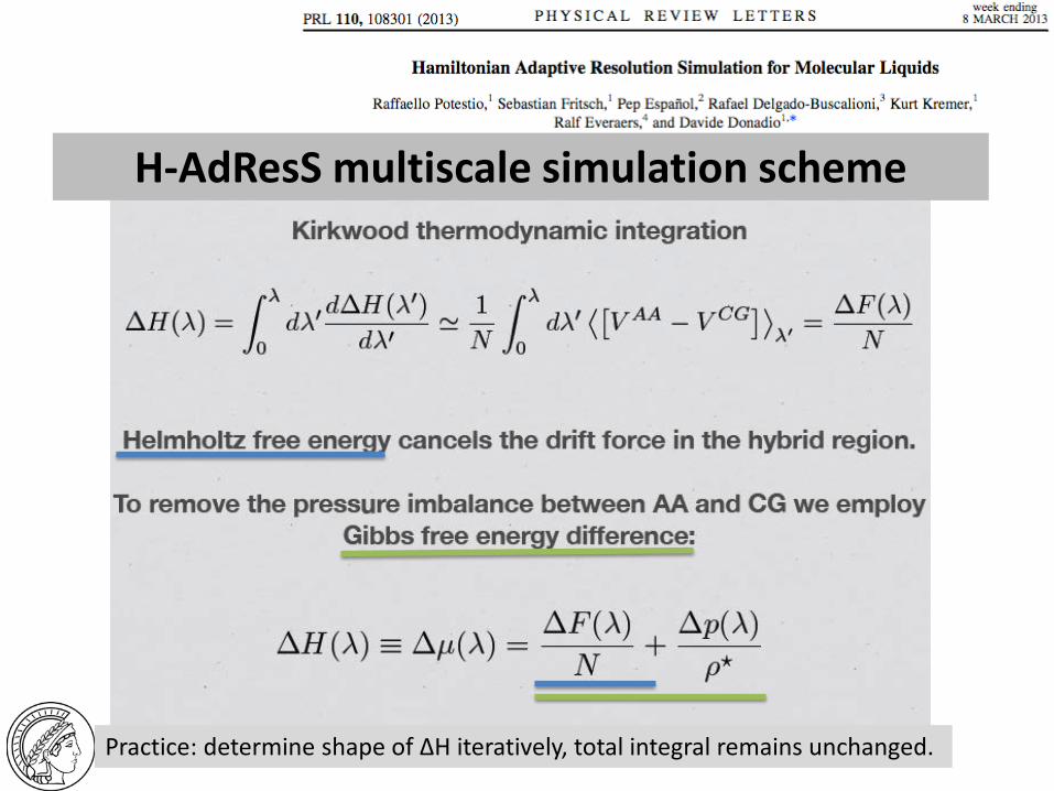
Potestio et. al., Phys. Rev. Lett. 110, 108301 (2013)
Fritsch et. al., Phys. Rev. Lett. 108, 170602 (2012)
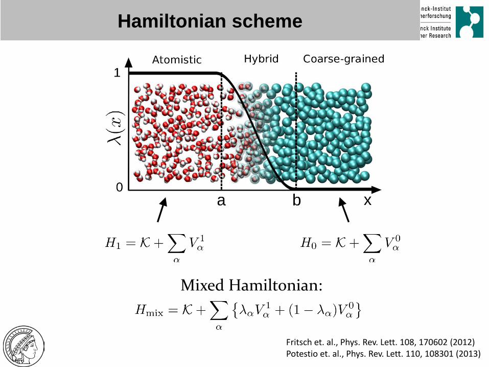
Hamiltonian scheme

Hamiltonian scheme
Idea: use weighted energy of each molecule and not forces

• Force interpolation:
• Additive force interpolation! Newton’s 3rd law fulfilled!
Potestio et. al., Phys. Rev. Lett. 110, 108301 (2013) Fritsch et. al., Phys. Rev. Lett. 108, 170602 (2012)
Energy Interpolation vs. Force Interpolation

Energy-based scheme leads to undesired drift force
Mixed Hamiltonian:
Forces:
• Model :
• Model : Potestio et. al., Phys. Rev. Lett. 110, 108301 (2013)
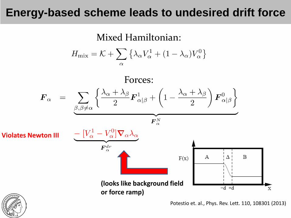
Energy-based scheme leads to undesired drift force
Mixed Hamiltonian:
Forces:
Potestio et. al., Phys. Rev. Lett. 110, 108301 (2013)
Violates Newton III
(looks like background field or force ramp)
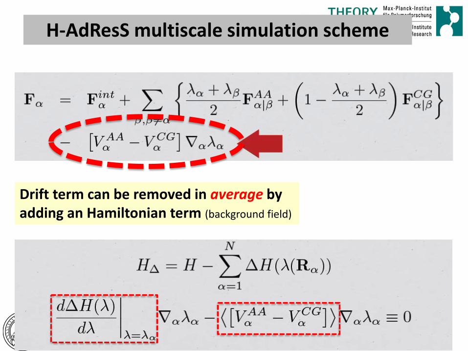
H-AdResS multiscale simulation scheme
Drift term can be removed in average by adding an Hamiltonian term (background field)
H-AdResS multiscale simulation scheme
Practice: determine shape of ΔH iteratively, total integral remains unchanged.

H-AdResS multiscale simulation scheme

H-AdResS multiscale simulation scheme

• Model :
• Model :
From H-AdResS to AdResS
Mixed Hamiltonian:
Forces:

Drift Forces decorrelate faster than Positions
• Position autocorrelation:
• Drift Force autocorrelation (averaged over all values for ):
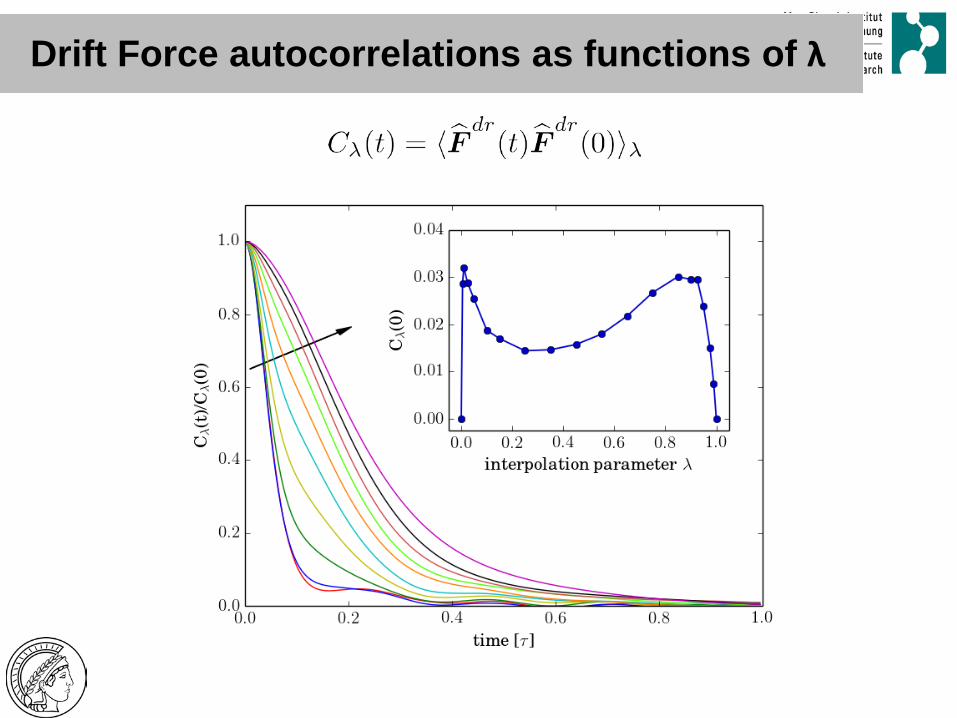
Drift Force autocorrelations as functions of λ
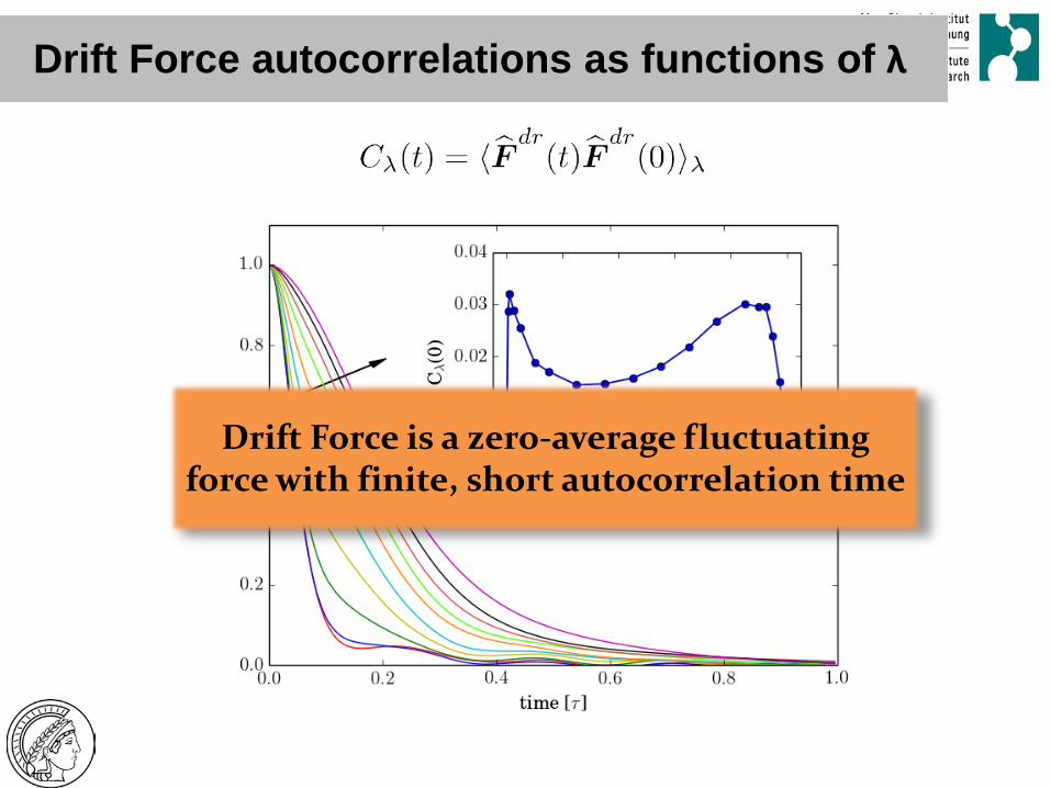
Drift Force is a zero-average fluctuating force with finite, short autocorrelation time
Drift Force autocorrelations as functions of λ
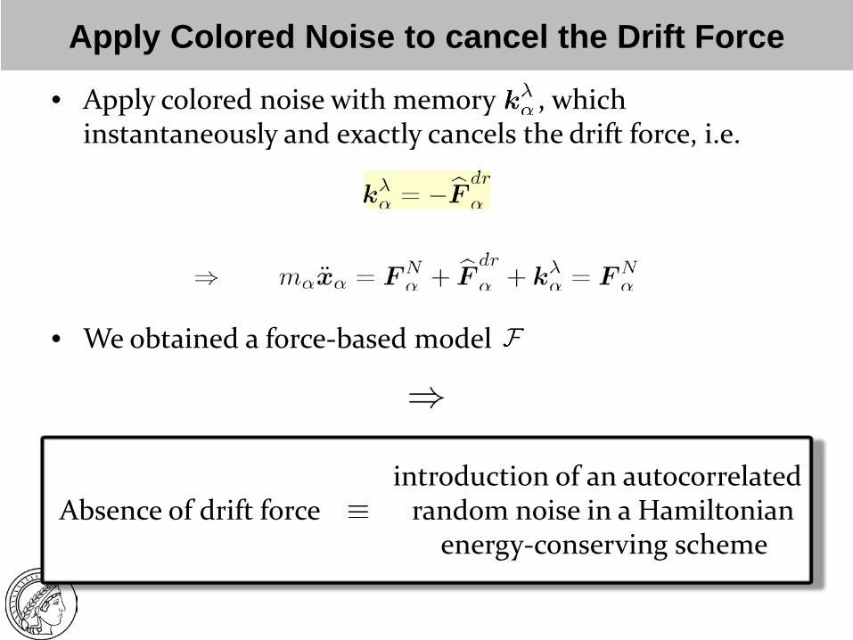
Apply Colored Noise to cancel the Drift Force
• Apply colored noise with memory , which instantaneously and exactly cancels the drift force, i.e.
• We obtained a force-based model
introduction of an autocorrelated Absence of drift force random noise in a Hamiltonian
energy-conserving scheme
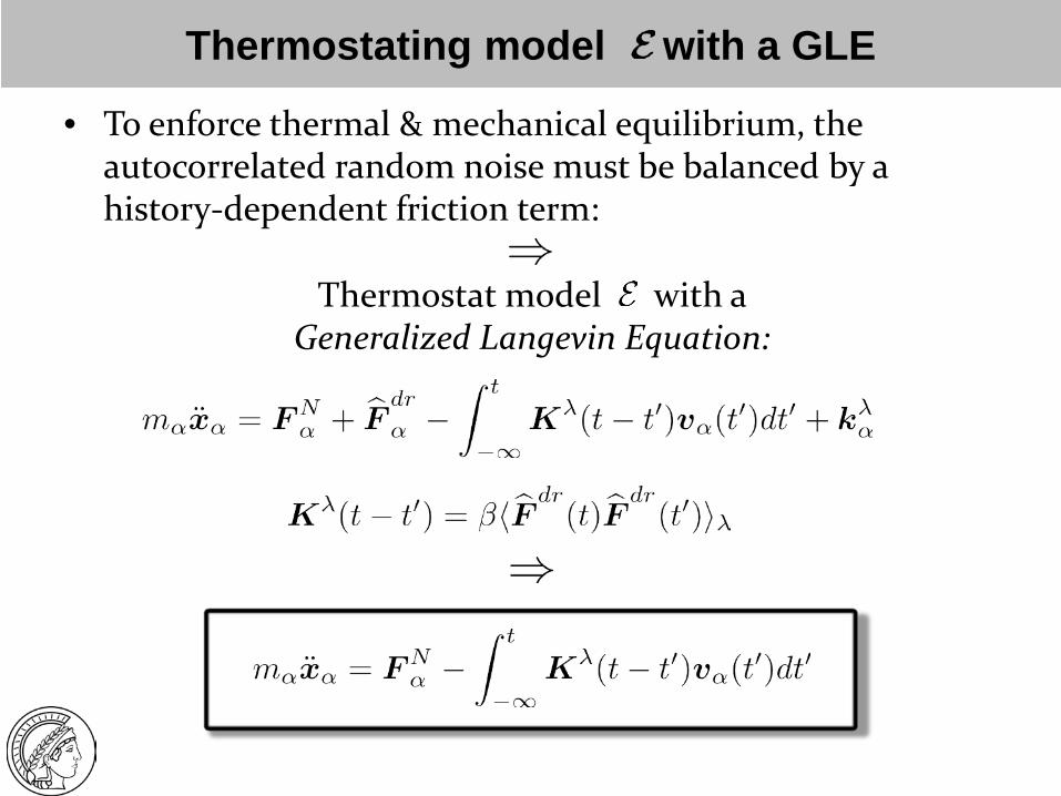
Thermostating model with a GLE
• To enforce thermal & mechanical equilibrium, the autocorrelated random noise must be balanced by a history-dependent friction term:
Thermostat model with a
Generalized Langevin Equation:
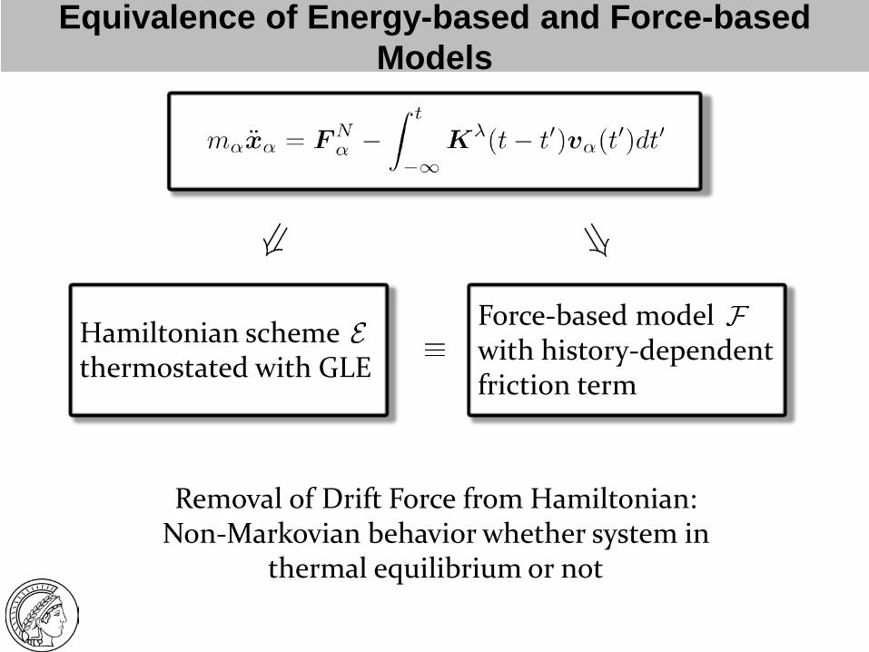
Equivalence of Energy-based and Force-based Models
Hamiltonian scheme thermostated with GLE
Force-based model with history-dependent friction term
Removal of Drift Force from Hamiltonian: Non-Markovian behavior whether system in
thermal equilibrium or not

Applications, Extensions
• Coupling to an ideal gas • Path integral quantum description • Large solutes in solvents • Cosolvent Effects for (Bio-) Polymers
‘stimuli responsive’ or ‘smart polymers’
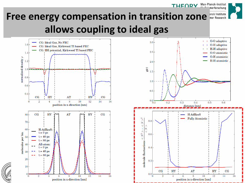
Free energy compensation in transition zone allows coupling to ideal gas
Applications, Extensions
• Coupling to an ideal gas • Path integral quantum description • Large solutes in solvents • Cosolvent Effects for (Bio-) Polymers
‘stimuli responsive’ or ‘smart polymers’

Path integral quantum AdResS
See also Argawall & Delle Site JCP et al 143, 094102 (2015 )

Path integral quantum AdResS
Classical – quantum: vary mass of particles in pearls
K. Kreis, M. Tuckerman, D. Donadio, KK, R. Potestio ,2015
Interpolate between quantum (light mass m) and classical particle (heavy mass M) 0 ≤ λ ≤ 1 Feynman: quantum particle as a classical ring polymer of light particles of mass m

Applications, Extensions
• Coupling to an ideal gas • Path integral quantum description • Large solutes in solvents • Cosolvent Effects for (Bio-) Polymers
‘stimuli responsive’ or ‘smart polymers’

Applications
• Large solutes in solvents • Cosolvent Effects for (Bio-) Polymers
‘stimuli responsive’ or ‘smart polymers’
Structure based Coarse Graining: Perfect match of g(r) all atom – coarse grained κatomistic = κcg BUT pcg = 6200patomistic
Test case: Coarse Grained Water: SPC/E
Compensation forces between regions needed
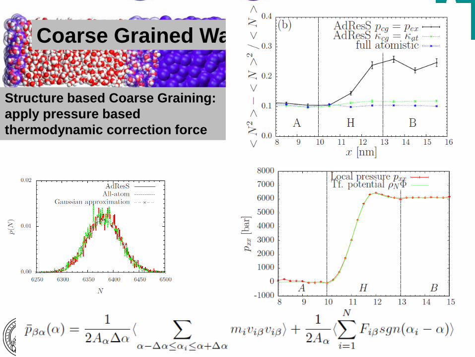
Coarse Grained Water: SPC/E
Structure based Coarse Graining: apply pressure based thermodynamic correction force

coarse grained hybrid explicit coarse grained hybrid explicit
Example SPC/E water
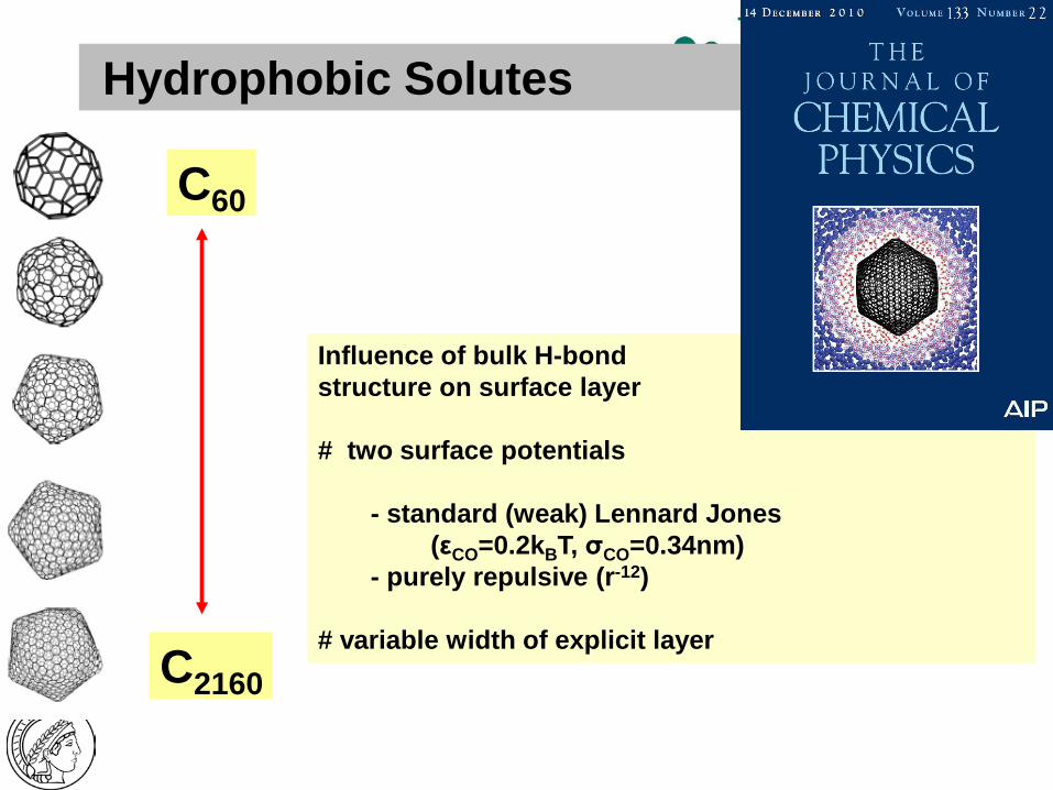
Hydrophobic Solutes
C60
C2160
Influence of bulk H-bond structure on surface layer # two surface potentials - standard (weak) Lennard Jones (εCO=0.2kBT, σCO=0.34nm) - purely repulsive (r-12) # variable width of explicit layer

Transition layer All atom layer, dex
Hydrophobic Solutes: Surface vs Bulk CG regime
Water
cg water reproduces g(r) but NOT tetrahedral packing!
B. P. Lambeth, C. Junghans, KK, C. Clementi, L. Delle Site, JCP 2010

Application: Ubiquitin in Water
• Ubiquitin in water, …
A. C. Fogarty, R. Postestio, KK, JCP 2015

• Ubiquitin in water, …
A. C. Fogarty, R. Postestio, KK, JCP 2015
Only TWO layers of explicit water needed to properly reproduce B-factors!
Application: Ubiquitin in Water

Application: HEWL - Hen Egg White Lysozyme Combining AdResS with Elastic Network Models
A. C. Fogarty, R. Postestio, KK, submitted 2015
ENM – AA model AdResS setup

Applications
• Large solutes in solvents • Cosolvent Effects for (Bio-) Polymers
‘stimuli responsive’ or ‘smart polymers’

Co (Non-) Solvency of Poly(NIPAm) in Water Alcohol Mixtures
- Water and alcohol are both good solvents - water and alcohol are miscible
Bischofberger et al. Soft Matter 10,8288 (2014)
‘good’ ‘poor’ ‘good solvent’
Temperature fixed

Co (Non-) Solvency of Poly(NIPAm) in Water Alcohol Mixtures
- Water and alcohol are both good solvents - water and alcohol are miscible
Bischofberger et al. Soft Matter 10,8288 (2014)
‘good’ ‘poor’ ‘good solvent’
Two mixed good solvents result in a poor solvent How can this be possible?
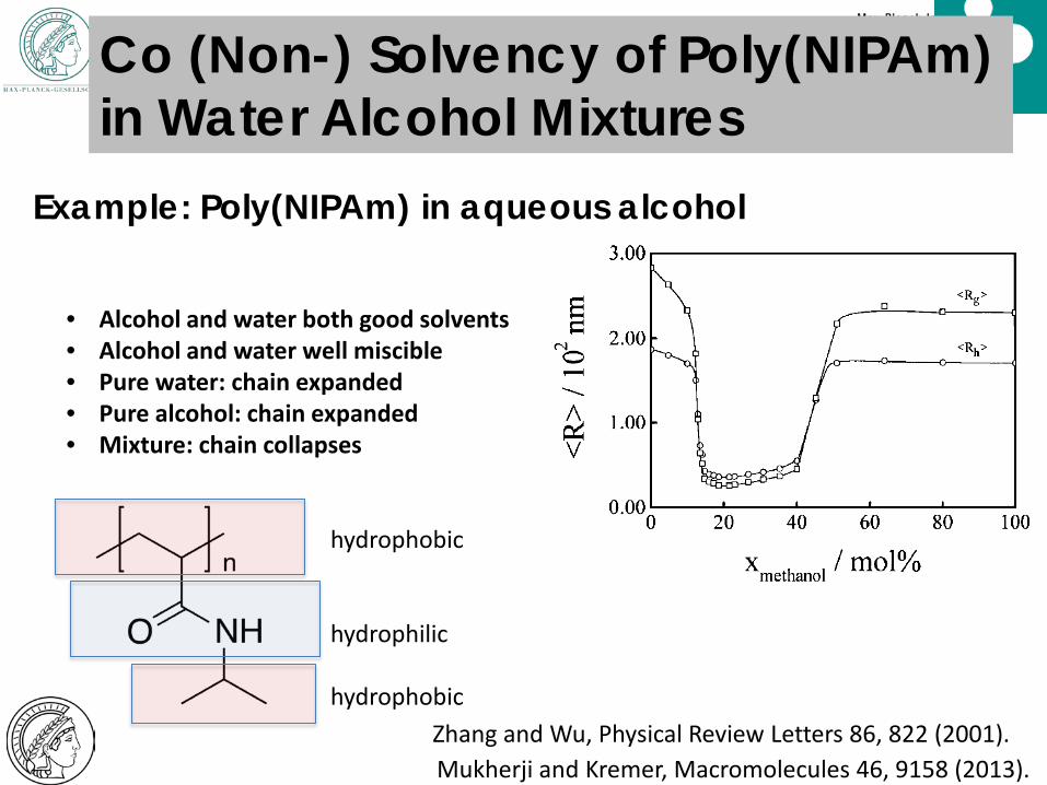
Example: Poly(NIPAm) in aqueous alcohol
Zhang and Wu, Physical Review Letters 86, 822 (2001). Mukherji and Kremer, Macromolecules 46, 9158 (2013).
• Alcohol and water both good solvents • Alcohol and water well miscible • Pure water: chain expanded • Pure alcohol: chain expanded • Mixture: chain collapses
hydrophobic hydrophilic hydrophobic
Co (Non-) Solvency of Poly(NIPAm) in Water Alcohol Mixtures

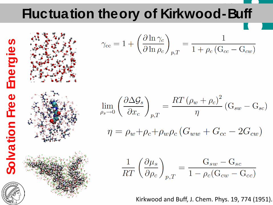
Fluctuation theory: Global thermodynamic properties from microscopic (pair-wise) molecular distributions
Kirkwood and Buff, J. Chem. Phys. 19, 774 (1951).
∆Nij = ρ jGij
Excess (depletion) coordination number ⇒ Grand canonical ensemble (or needs very large systems)
- Solvation energy - Partial molar volume - Activity coefficient - Compressibility …….
Fluctuation theory of Kirkwood-Buff
Fluctuation theory of Kirkwood-Buff So
lvat
ion
Free
Ene
rgie
s
Kirkwood and Buff, J. Chem. Phys. 19, 774 (1951).
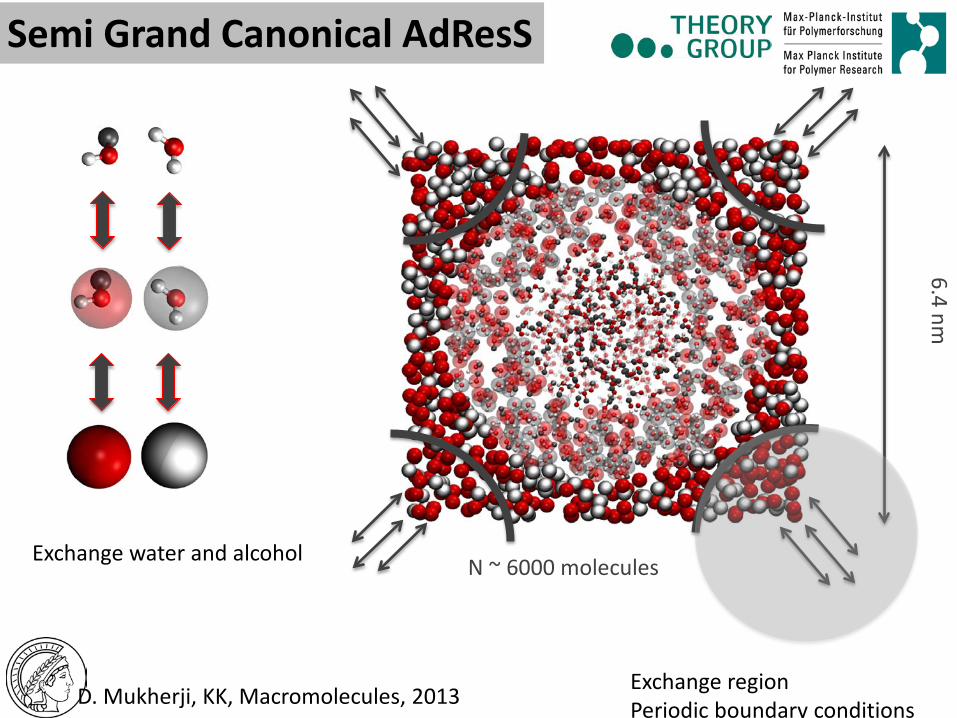
Semi Grand Canonical AdResS
D. Mukherji, KK, Macromolecules, 2013
Exchange water and alcohol
6.4 nm
N ~ 6000 molecules
Exchange region Periodic boundary conditions

Semi Grand Canonical AdResS
D. Mukherji, KK, Macromloecules, 2013
Exchange water and alcohol
6.4 nm
N ~ 6000 molecules
Exchange region Periodic boundary conditions

Poly-NIPAm chemical potential shift
“expected shape”
Mukherji and Kremer, Macromolecules (2013)
100% water 100% alc.

“expected shape”
Mukherji and Kremer, Macromolecules (2013)
Poly-NIPAm chemical potential shift
100% water 100% alc.
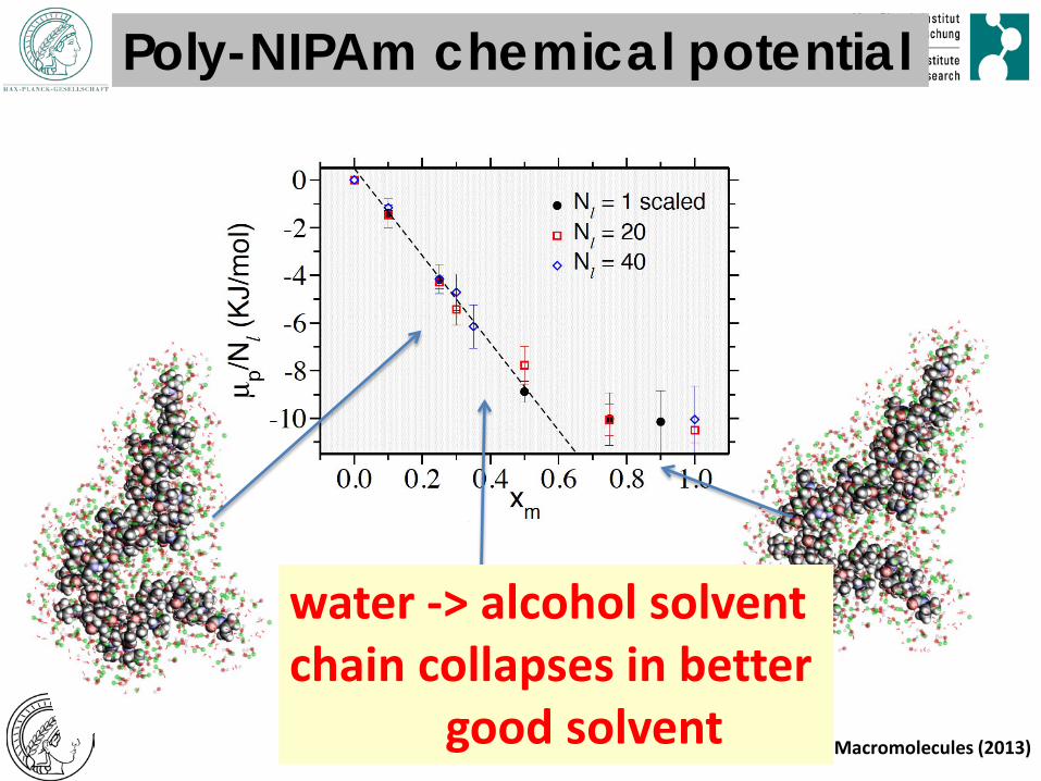
Poly-NIPAm chemical potential
Mukherji and Kremer, Macromolecules (2013)
water -> alcohol solvent chain collapses in better good solvent

Poly-NIPAm in aqueous methanol
Mukherji, KK, Macromolecules (2013) Mukherji, Marques,KK, Nat. Comm. (2014), JCP (2015)

Conclusion / Challenges
• Dual-Triple… Scale Simulations/Theory – Adaptive quantumforce fieldcoarse grained … – Grand Canonical i.e. salt etc
• Nonbonded Interactions: NEMD, Structure Formation, Morphology…
• Conformations Electronic/Optical Properties • Structure Formation, Aggregation, Dynamics • Online Experiments:
– Nanoscale Experiments, long Times
Materials are the result of non equilibrium processes
PostDoc and PhD Student positions available http://www.mpip-mainz.mpg.de/polymer_theory
Top Related