


Languages
Pages
Legal


MULTISCALE MODELING OF REACTIVE
Ni/Al NANOLAMINATES
by
Leen Alawieh
A dissertation submitted to The Johns Hopkins University in conformity with the
requirements for the degree of Doctor of Philosophy.
Baltimore, Maryland
October, 2013
c© Leen Alawieh 2013
All rights reserved
Abstract
This dissertation employs multiscale modeling for the purpose of investigating
reactions occurring in reactive Ni/Al nanolaminates. These are comprised of alter-
nating layers of Ni and Al that can react exothermically upon local ignition, even-
tually leading to the initiation of a self-propagating reaction front with speeds that
can exceed 10 m/s. A generalized thermal transport model is developed, based on
the transient multi-dimensional reduced continuum formalism introduced by Salloum
and Knio [31]. The generalized model accounts for an anisotropic thermal conduc-
tivity, that also depends on composition and temperature. A systematic analysis of
the role and ramifications that such a generalization has on the flame front structure
and dynamics is conducted, revealing that it has a dramatic impact on the ability to
successfully capture experimentally observed thermal front instabilities.
A multiscale analysis is then conducted in order to infer atomic intermixing rates
prevailing during different reaction regimes in the nanolaminates. The analysis com-
bines the results of Molecular Dynamics (MD) simulations with macroscale experi-
mental observations, and leads to the construction of a new composite atomic dif-
ii

ABSTRACT
fusivity law. Using this composite diffusivity law, a generalized reduced model is
obtained with the capability to simultaneously capture various reaction mechanisms
over a wide temperature range.
The generalized reduced model for single multilayers is then extended towards
exploring reactions occurring in layered particle networks. A further reduction of the
model is sought through identifying regimes under which spatial homogenization on
the particle level would be valid. The limiting case of a single chain of particles is
considered, and comparisons between the computational results of the heterogeneous
and the homogeneous reduced model descriptions are carried out. These reveal a
complex dependence of the reaction progress on the system properties and that simple
scaling arguments, based on particle size and rates of heat transfer, are not sufficient
for establishing a universal criterion of validity.
Advisor: Professor Omar M. Knio
Readers: Professor Timothy P. Weihs
Readers: Professor Joseph Katz
iii
Acknowledgments
First and foremost, I would like to express my sincere gratitude to my advisor,
Professor Omar M. Knio, for providing me with the opportunity to join his group,
and learn about reactive materials and numerical modeling in general. His endless
enthusiasm, stimulating discussions, guidance, patience, and support have been inte-
gral to this work. I cannot thank him enough for his kindness and all that he has
taught me over the past few years. I have been privileged to be his student.
I would also like to extend my deep appreciation to Professor Timothy P. Weihs
for his continuous insightful feedback on my work, and for providing me with the
experimental data that I needed to carry out my research. I am also thankful to
Professor Joseph Katz for serving as a member of my Ph.D. defense committee, and
as a reader for this dissertation.
For helping fund the work in this dissertation, I am grateful for the U.S. Depart-
ment of Energy, Office of Basic Energy Sciences, Division of Materials Sciences and
Engineering Award DE-SC0002509; the Office of Naval Research Award N00014-07-1-
0740; and the Defense Threat Reduction Agency, Basic Research Award # HDTRA1-
iv
ACKNOWLEDGMENTS
11-1-0063.
I want to also thank Professors Todd C. Hufnagel, Michael L. Falk, Takeru Igusa,
Cila Herman, and Sean X. Sun for their encouragement and interesting discussions. I
am especially appreciative of Professors Hufnagel’s and Falk’s constructive input on
my work during the group meetings, and of Professor Falk’s and Mr. Rong-Guang
Xu’s invaluable help with initializing the Molecular Dynamics simulations when I first
embarked on the atomistic investigations.
Credit also goes to all the staff members in the Mechanical Engineering department
for making the annoying administrative issues much easier to deal with.
I am deeply grateful for my friends and colleagues here at Hopkins and elsewhere.
Without the fun moments, their help and support, graduate school would have been a
much less rich, memorable, and enjoyable experience. Special thanks to my childhood
and college friends back in Lebanon for all the past, and ongoing, stimulating and
heart-warming moments.
Last but not least, I am profoundly indebted to my family for their unconditional
love and unwavering support. Without them, none of this would have been possible.
v

Dedication
For a better understanding of nature.
vi
Contents
Abstract ii
Acknowledgments iv
List of Tables x
List of Figures xi
1 Introduction 1
1.1 Ni/Al Nanolaminates . . . . . . . . . . . . . . . . . . . . . . . . . . . 4
1.1.1 Multilayer Fabrication . . . . . . . . . . . . . . . . . . . . . . 4
1.1.2 Reaction Basics . . . . . . . . . . . . . . . . . . . . . . . . . . 5
1.1.3 Reaction Initiation and Self-Propagation . . . . . . . . . . . . 7
1.1.4 Scientific Motivations and Applications . . . . . . . . . . . . . 9
1.2 Outline . . . . . . . . . . . . . . . . . . . . . . . . . . . . . . . . . . . 10
2 Methodology 13
vii

CONTENTS
2.1 Multilayer configuration . . . . . . . . . . . . . . . . . . . . . . . . . 13
2.2 Continuum Model . . . . . . . . . . . . . . . . . . . . . . . . . . . . . 16
2.3 Model Reduction . . . . . . . . . . . . . . . . . . . . . . . . . . . . . 19
2.4 Numerical Scheme . . . . . . . . . . . . . . . . . . . . . . . . . . . . 22
3 Effects of Thermal Diffusion 25
3.1 Motivation . . . . . . . . . . . . . . . . . . . . . . . . . . . . . . . . . 25
3.2 Derivation of the generalized thermal transport models . . . . . . . . 28
3.2.1 Constant κ . . . . . . . . . . . . . . . . . . . . . . . . . . . . 29
3.2.2 Concentration dependent κ . . . . . . . . . . . . . . . . . . . 30
3.2.3 Direction-dependent κ . . . . . . . . . . . . . . . . . . . . . . 30
3.2.4 Direction and temperature dependent κ . . . . . . . . . . . . . 33
3.3 Results . . . . . . . . . . . . . . . . . . . . . . . . . . . . . . . . . . . 45
3.3.1 Front Properties . . . . . . . . . . . . . . . . . . . . . . . . . 46
3.3.2 Axial Front Structure . . . . . . . . . . . . . . . . . . . . . . . 47
3.3.3 Normally-Propagating Fronts . . . . . . . . . . . . . . . . . . 56
3.3.4 3D computations . . . . . . . . . . . . . . . . . . . . . . . . . 61
4 Inference of Atomic Diffusivity 66
4.1 Motivation . . . . . . . . . . . . . . . . . . . . . . . . . . . . . . . . . 66
4.2 Atomistic Simulations . . . . . . . . . . . . . . . . . . . . . . . . . . 68
4.2.1 Coarse graining . . . . . . . . . . . . . . . . . . . . . . . . . . 71
viii

CONTENTS
4.2.2 Extracting D(T ) . . . . . . . . . . . . . . . . . . . . . . . . . 72
4.3 Results . . . . . . . . . . . . . . . . . . . . . . . . . . . . . . . . . . . 75
4.3.1 MD analysis . . . . . . . . . . . . . . . . . . . . . . . . . . . . 76
4.4 Macroscale Information . . . . . . . . . . . . . . . . . . . . . . . . . . 89
4.4.1 Low Temperature Regime . . . . . . . . . . . . . . . . . . . . 89
4.4.2 Intermediate Temperature Regime . . . . . . . . . . . . . . . . 95
4.4.3 High Temperature Regime . . . . . . . . . . . . . . . . . . . . 102
4.5 Discussion . . . . . . . . . . . . . . . . . . . . . . . . . . . . . . . . . 111
5 Reactive Multilayered Particles 116
5.1 Motivation . . . . . . . . . . . . . . . . . . . . . . . . . . . . . . . . . 116
5.2 Problem Formulation and Approach . . . . . . . . . . . . . . . . . . . 127
5.3 Results . . . . . . . . . . . . . . . . . . . . . . . . . . . . . . . . . . . 132
6 Conclusions 149
Bibliography 154
Vita 177
ix

List of Tables
x

List of Figures
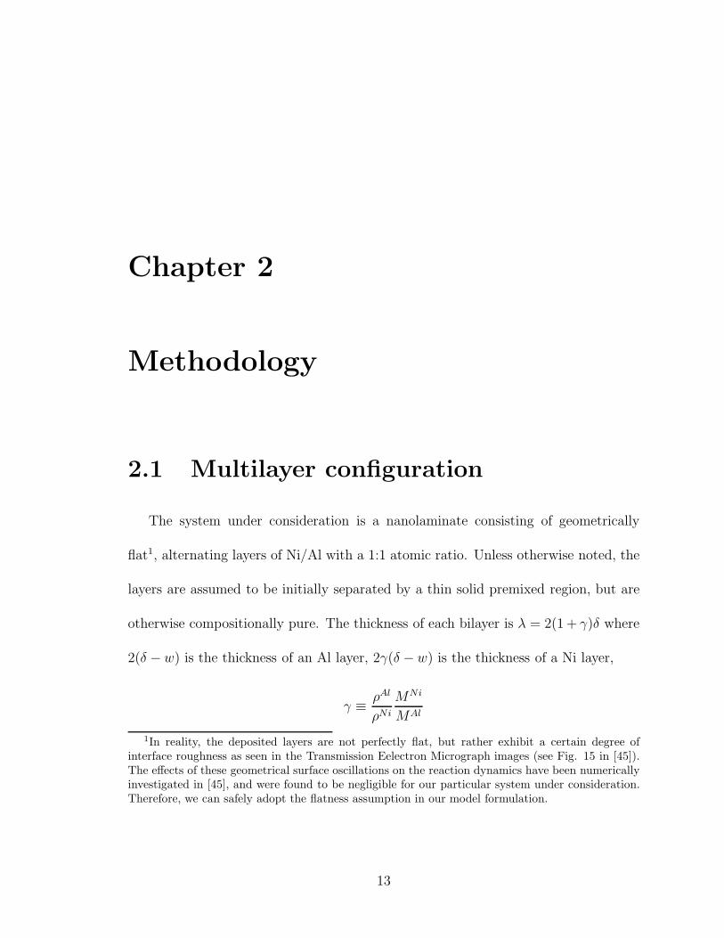
2.1 2D schematic of an unreacted (1:1) Ni/Al bilayer separated by a thinNiAl premix region. The total thickness of the bilayer is λ = 2(1+γ)δ,where the Al, Ni, and premix layers have individual thicknesses of2(δ − w), 2γ(δ − w), and 4w, respectively. . . . . . . . . . . . . . . . 15
3.1 Thermal conductivity of pure Al as a function of temperature. Shownare data from Touloukian et al. [99], along with the two best fits forthe solid and liquid states of Al. The melting temperature indicatedin the plot is 933K approximately; R2 ≈ 0.9992 for the fit in the solidstate, whereas R2 ≈ 0.9998 for the one in the liquid state region. . . . 35
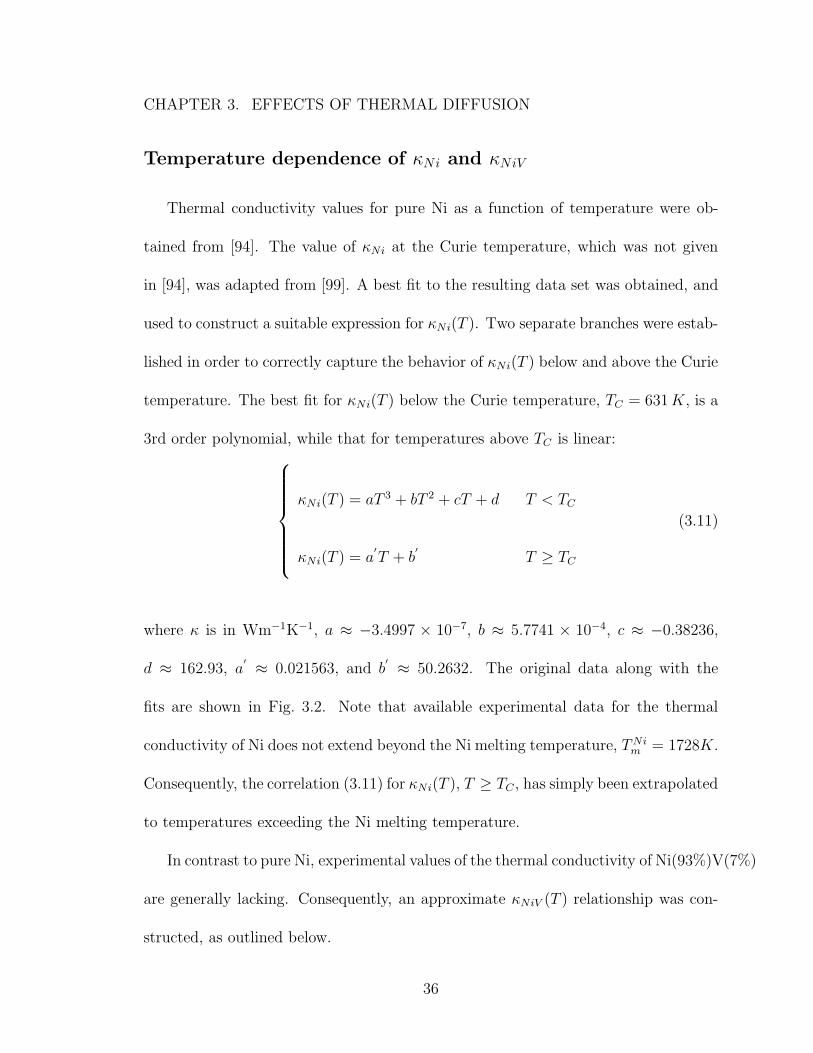
3.2 Thermal conductivity of pure Ni as a function of temperature. Shownare the original data reported in [94] along with the best two fits forthe data below and above the Ni Curie temperature, TC ≈ 631K.The value of κNi at TC has been obtained from [99]. R2 ≈ 0.9997 forT < TC , whereas R
2 ≈ 0.9999 for T ≥ TC . . . . . . . . . . . . . . . . 373.3 Thermal conductivity of stoichiometric NiAl as a function of tempera-
ture. Shown are the data reported by Terada et al. [97] along with thebest fit for the data. R2 ≈ 0.9955. . . . . . . . . . . . . . . . . . . . . 41
3.4 Thermal conductivity of Ni(48%)V(2%)Al(50%) as a function of tem-perature. Shown are the data reported by Terada et al. [97] along withthe best fit for the data. R2 ≈ 0.9993. . . . . . . . . . . . . . . . . . . 42
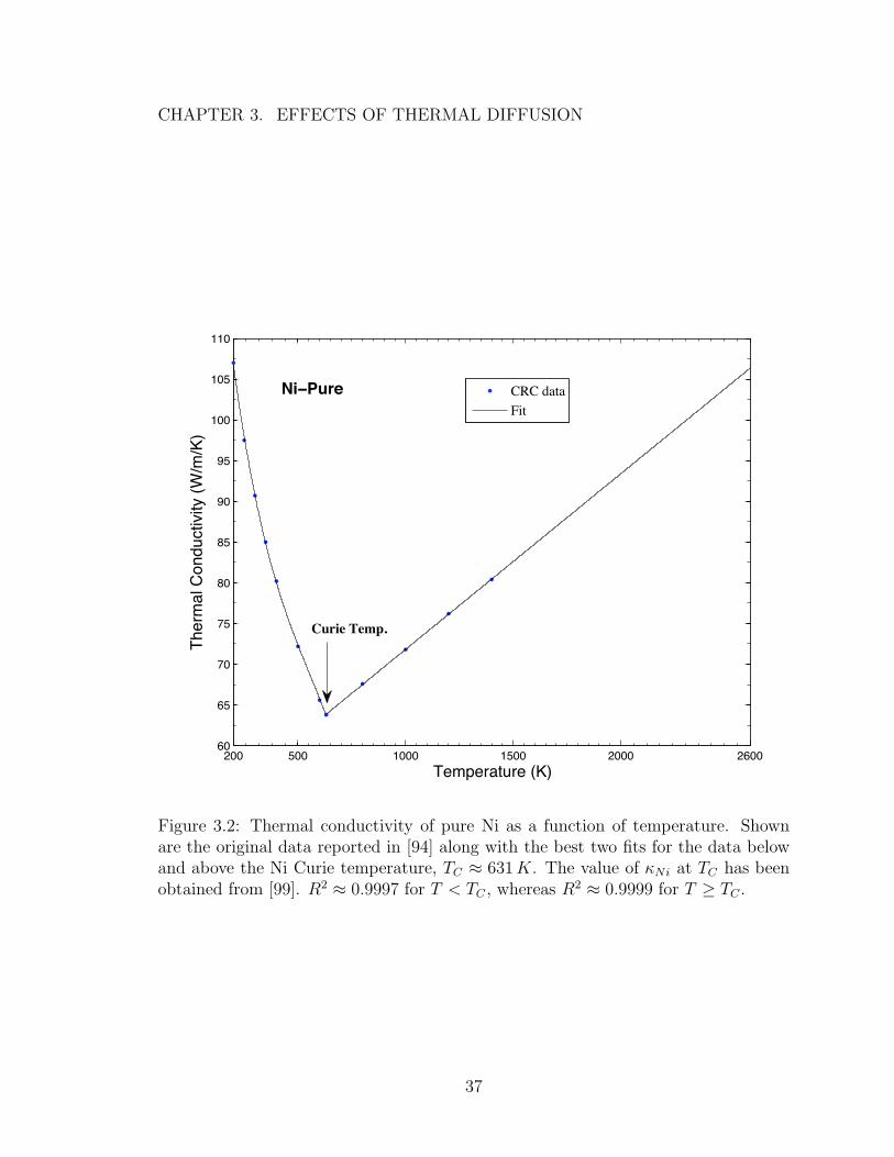
3.5 Dependence of κ on temperature, direction, and concentration. Thesolid and dashed line plots correspond to thermal conductivity of pureNi/Al multilayers along the axial (x and z) and normal (y) directions,evaluated using (3.6) and (3.7) respectively. Curves are generated fordifferent values of C, as indicated. The (N) symbol refers to the valueof κ for the constant conductivity model computed using (3.2). . . . . 43
xi

LIST OF FIGURES
3.6 Dependence of κ on temperature, direction, and concentration. Thesolid and dashed line plots correspond to thermal conductivity of NiV/Almultilayers along the axial (x and z) and normal (y) directions, eval-uated using (3.8) and (3.9) respectively. Curves are generated for dif-ferent values of C, as indicated. The (N) symbol refers to the value ofκ for the constant conductivity model, computed using (3.3). . . . . . 44
3.7 Thermal width of the front versus δ. Curves are generated for Ni/Al(solid) and NiV/Al (dashed) multilayers, using the constant, concentration-dependent, and concentration and temperature dependent κ models,as indicated. Inset shows a zoom in on the region of δ = 12− 72 nm. 48
3.8 Reaction width of the front versus δ. Curves are generated for Ni/Al(solid) and NiV/Al (dashed) multilayers, using the constant, concentration-dependent, and concentration and temperature dependent κ models,as indicated. Inset shows a zoom in on the region of δ = 12− 72 nm. 50
3.9 Average, 1D, axial flame velocity versus δ. Curves are generated forNi/Al (solid) and NiV/Al (dashed) multilayers using the constant,concentration-dependent, and concentration and temperature depen-dent κ models, as indicated. In all cases, w = 0.8 nm. . . . . . . . . . 52
3.10 Average, 1D, axial flame velocity versus σR. Curves are generated forNi/Al (solid) and NiV/Al (dashed) multilayers, using the constant,concentration-dependent, and concentration and temperature depen-dent κ models, as indicated. The same data points as in Figs. (3.8)and (3.9) are used. . . . . . . . . . . . . . . . . . . . . . . . . . . . . 54
3.11 Normalized average scalar concentration, C/C0 versus the normalizedtemperature T/Tf . The scatter plot depicts results for Ni/Al multilay-ers, obtained for different values of δ using the constant, concentration-dependent, and concentration and temperature-dependent κmodels, asindicated. Note that the temperature band observed on the C = 0 axisincludes superadiabatic overshoots that are associated with transientfront propagation [45]. . . . . . . . . . . . . . . . . . . . . . . . . . . 55
3.12 Reaction width versus δ. Curves are generated for axial and normalfront propagation in Ni/Al multilayers, using the (i) constant, (ii) con-centration dependent, (iii) concentration and direction dependent, and(iv) concentration, direction and temperature dependent κ models, asindicated. . . . . . . . . . . . . . . . . . . . . . . . . . . . . . . . . . 58
3.13 Average front velocity versus δ. Curves are generated for axial andnormal front propagation in Ni/Al multilayers, using the (i) constant,(ii) concentration dependent, (iii) concentration and direction depen-dent, and (iv) concentration, direction and temperature dependent κmodels, as indicated. . . . . . . . . . . . . . . . . . . . . . . . . . . . 59
xii
LIST OF FIGURES
3.14 Instantaneous distributions of surface temperature. The 3D computa-tions are performed for Ni/Al multilayer with δ = 6 nm, using the tem-perature dependent κ model over a domain size of (Lx×Lz ×Ly) = (1mm ×1 mm ×10µm). Ignition was simulated by imposing a surfaceheat flux for a short duration over a small square region centered at0.1
√2 mm from the origin. . . . . . . . . . . . . . . . . . . . . . . . . 63
3.15 Instantaneous surface heat release rate profiles. The 3D computationsare performed for Ni/Al multilayer with δ = 75 nm, using the directiondependent κ model over a domain size of (Lx × Lz × Ly) = (1 mm ×1mm ×2µm). Ignition was simulated by imposing a surface heat fluxfor a short duration over a small square region centered at 0.1
√2 mm
from the origin. . . . . . . . . . . . . . . . . . . . . . . . . . . . . . . 64
4.1 Snapshot of the initial configuration of Ni (white) and Al (green) atomsin the MD system at time t = 0. The arrangement corresponds to aNi/Al bilayer of total thickness λ = 8 nm and δ = 2.34 nm. . . . . . . 70
4.2 Cumulative distribution functions (CDF) of Nickel (red) and Alu-minum (blue), computed at (a) t = 0, and (b) t = 2.2 × 10⁴ psec.The dashed line y = x corresponds to the asymptotic limit of a com-pletely mixed system. . . . . . . . . . . . . . . . . . . . . . . . . . . . 78
4.3 Mixing measure versus time for an MD system with δ = 2.34 nm. Thecurves depicts the evolution of M(t) during the initial equilibrationstage, the rapid heating stage to T = 700 K, and the adiabatic stage.Inset provides an enlarged view of the late stages of the computations,during which the Ni structure collapses. . . . . . . . . . . . . . . . . . 79
4.4 Average temperature versus time for an MD system with δ = 2.34 nm.The curves depicts the evolution of T (t) during the initial equilibrationstage, the rapid heating stage to T = 700 K, and the adiabatic stage.Inset provides an enlarged view of the late stages of the computations,during which the Ni structure collapses. . . . . . . . . . . . . . . . . . 80
4.5 Inferred diffusivity versus temperature. Plotted are curves generatedfor MD systems with δ = 2.34 nm (blue) and δ = 4.78 nm (black). Thetemperature range corresponds to the adiabatic stage in Figure 4.4.The solid curves correspond to approximations obtained as best fits tothe inferred D(T ) values obtained for δ = 2.34 nm along three separatebranches. . . . . . . . . . . . . . . . . . . . . . . . . . . . . . . . . . 82
xiii

LIST OF FIGURES
4.6 Mixing measure versus time for the MD system with δ = 2.34 nm,under homogeneous, adiabatic reaction conditions. The blue curvecorresponds to the MD data shown in Figure 4.3 during the adiabaticstage, whereas the red dashed curve corresponds to predictions usingthe reduced continuum model with the approximate D(T ) fits depictedin Figure 4.5. Note that the continuum model does not take intoaccount the initial premixing that had occurred in MD during theheating stage, and instead starts from a purely unmixed state M(t =0) = 1. . . . . . . . . . . . . . . . . . . . . . . . . . . . . . . . . . . 84
4.7 Average potential energy of the MD system with δ = 2.34 nm ver-sus the mixing measure, M , during the adiabatic phase.The M valuescorrespond to those shown in Fig. 4.3 during the adiabatic stage. . . . 86
4.8 Temperature evolution with time for a homogeneous reaction regimein a NiV/Al multilayer with δ = 56 nm. The blue curve correspondsto experimental observations by Fritz [19], while the red dashed curvecorresponds to predictions (truncated at T = 800 K) using the reducedcontinuum model with optimized pre-exponent and activation energyvalues, D0 = 2.08×10⁻⁷m2/s and Ea = 92.586 kJ/mol. Inset providesa zoom into the optimized region following the heating stage. . . . . . 92
4.9 Comparison between the D(T ) correlation obtained by Fritz [19] withD0 = 5.58× 10⁻⁹m2/s and Ea = 78.9 kJ/mol (red dashed curve), andthose obtained using the reduced continuum model with optimizedpre-exponent and activation energy values, D0 = 2.08×10⁻⁷m2/s andEa = 92.586 kJ/mol (solid black curve) and D0 = 5.176 × 10⁻⁸m2/sand Ea = 88.796 kJ/mol (green dashed curve) when assuming either alinear or a quadratic Q(C), respectively. . . . . . . . . . . . . . . . . 93
4.10 Inferred diffusivity, D, versus temperature, T . The estimates rely onthe experimental measurements of [106] for a nanocalorimeter incor-porating a Ni/Al bilayer with δ = 15 nm and a variant of the thermalmodel developed in [107]. Inset shows that the inferred D(T ) data inthe temperature range of interest does not exhibit an Arrhenius rela-tionship when plotted as ln(D) versus 1/T , and that rather the naturallogarithm of a quadratic fit, shown by the red solid curve, would bemore appropriate. . . . . . . . . . . . . . . . . . . . . . . . . . . . . . 99
4.11 Combined extracted D(T ) values (on a semi-log scale) in the low andintermediate temperature regimes. The blue data points were plottedusing the Arrhenius diffusivity parameters optimized in Figure 4.8,while the red circles were plotted using the quadratic fit shown in theinset of Figure 4.10. Inset provides a zoom near the overlap regionbetween the D(T ) predictions (on a linear scale) using the outcomes ofthe low temperature regime optimization and that of the intermediatetemperature regime inference. . . . . . . . . . . . . . . . . . . . . . . 101
xiv

LIST OF FIGURES
4.12 Average axial self-propagating flame velocities as a function of δ on thebottom axis and λ on the top axis. The blue dots and error bars corre-spond to experimental observations of Knepper et al. [29], whereas theopen circles and red dots correspond to predictions using the reducedcontinuum model with optimized pre-exponent and activation energyvalues, D0 = 2.56× 10⁻⁶m2/s and Ea = 102.1910 kJ/mol in the hightemperature range, concurrently with the optimized and inferredD val-ues reported in Figures 4.8 and 4.10 at the lower temperatures. Theopen circles were obtained using a mesh size of ∆x = 0.5 µm, whereasthe red dots were obtained using a coarser mesh of size ∆x = 1 µm.Inset shows the variation of the finer-mesh velocity predictions whentaking smaller δ increments around the region where a velocity plateauis observed. . . . . . . . . . . . . . . . . . . . . . . . . . . . . . . . . 106
4.13 Temperature profiles along the foil length (direction of front propaga-tion) at the time instant t = 97.445 µs for δ values around the regionwhere there is a shoulder (plateau) in the reduced model velocity pre-dictions reported in Fig. 4.12. Also shown for comparison are thetemperature profiles at the time instants t = 55.645 µs for δ = 3 nmand δ = 5.3 nm, and t = 79.945 µs for δ = 9.1 nm. . . . . . . . . . . 108
4.14 Average axial self-propagating flame velocities as a function of δ onthe bottom axis and λ on the top axis. The blue dots correspondto experimental observations by Knepper [29], while the open circlesand red dots correspond to predictions using the reduced continuummodel. The open circles correspond to the open circle data pointsshown in Fig. 4.12 obtained using a premix width w = 0.8 nm. Thered data points were obtained for a premix width w = 0.91 nm with are-optimized pre-exponent and activation energy values, D0 = 1.91 ×10⁻⁶m2/s and Ea = 97.103 kJ/mol in the high temperature range,concurrently with the optimized and inferred D values reported inFigures 4.8 and 4.10 at the lower temperatures. The arrows highlightthe points where a velocity plateau is exhibited in both cases, and thered line provides a guide for the eye. . . . . . . . . . . . . . . . . . . 110
4.15 Final composite atomic diffusivity, D, values as a function of temper-ature combining results reported in Figures 4.8 – 4.12. Also shownfor comparison are the D(T ) values inferred from the MD simulationsreported in Figure 4.5 for δ = 2.34 nm, and the original global Ar-rhenius correlation obtained in [42] with D0 = 2.18 × 10⁻⁶m2/s andEa = 137 kJ/mol . . . . . . . . . . . . . . . . . . . . . . . . . . . . . 112
xv
LIST OF FIGURES
5.1 Normalized peak values of the instantaneous maximum and minimumtemperature differences in a given particle, Smax, as a function of ther-mal contact resistance Rc. Plotted are curves corresponding to differ-ent values of particle size, L, and half-layer thickness, δ. Solid lineswith solid dots correspond to δ = 50 nm, while dashed lines with opencircles correspond to δ = 250 nm. . . . . . . . . . . . . . . . . . . . . 136
5.2 Normalized time average of the instantaneous maximum and minimumtemperature differences in a given particle, < S(t) >, as a function ofthermal contact resistance Rc. Plotted are curves corresponding todifferent values of particle size, L, and half-layer thickness, δ. Solidlines with solid dots correspond to δ = 50 nm, while dashed lines withopen circles correspond to δ = 250 nm. . . . . . . . . . . . . . . . . 137
5.3 Relative time error in the reaction progress between the meshed andhomogeneous computations as a function of thermal contact resistanceRc. Plotted are curves corresponding to different values of particle size,L, and half-layer thickness, δ. Solid lines with solid dots correspondto δ = 50 nm, while dashed lines with open circles correspond toδ = 250 nm. Inset shows the same data points plotted on a log-log scale.141
5.4 Relative time error in the reaction progress between the meshed andhomogeneous computations as a function of Smax. Shown are curvescorresponding to different values of L, Rc, and δ. Solid lines with soliddots correspond to δ = 50 nm, while dashed lines with open circlescorrespond to δ = 250 nm. Both sets of data points correspond tothose shown in Figs. (5.1) and (5.3). . . . . . . . . . . . . . . . . . . 142
5.5 Relative time error in the reaction progress between the meshed andhomogeneous computations as a function of < S(t) >. Shown arecurves corresponding to different values of L, Rc, and δ. Solid lineswith solid dots correspond to δ = 50 nm, while dashed lines with opencircles correspond to δ = 250 nm. Both sets of data points correspondto those shown in Figs. (5.2) and (5.3). . . . . . . . . . . . . . . . . . 143
5.6 Relative time error, terror, as a function of the non-dimensional ratio ofthe particle’s internal thermal resistance, L/κ, to its thermal contactresistance, Rc. Shown are curves corresponding to different values ofL, Rc, and δ. Solid lines with solid dots correspond to δ = 50 nm,while dashed lines with open circles correspond to δ = 250 nm. Insetprovides a close-up into the region of small error and high Rc values. 145
xvi
LIST OF FIGURES
5.7 3D plot of terror as a function of L/κRc and the non-dimensional ratioof particle size to thermal front width, L/σT . Shown are curves cor-responding to different values of L, Rc, and δ. Solid lines with soliddots correspond to δ = 50 nm, while dashed lines with open circlescorrespond to δ = 250 nm. σT = 100 µm for δ = 250 nm and 20 µmfor δ = 50 nm. The terror 2D slice helps highlight the points at whichthe curves cross the 10% error threshold. . . . . . . . . . . . . . . . . 146
xvii
Chapter 1
Introduction
Most of the matter in nature is not in a state of equilibrium, but is rather under-
going constant change either through physical processes, chemical reactions, or both.
Systems that are seemingly in a stable equilibrium, could be driven out of this stag-
nant state after applying a sufficiently large perturbation as witnessed for example
by extreme occurrences such as avalanches, sinkholes, and fractures, or everyday oc-
currences such as ice formation, photosynthesis, and lightning. Energetic materials,
which are the focus of this dissertation, are intimately related to another instance of
such events, namely combustion.
Combustion typically involves the reaction, after a certain degree of initial heating,
of hydrocarbons (or simply solid carbon) and oxygen to form carbon dioxide, water
vapor, and other possible byproducts, along with the release of a certain amount
of heat. This phenomenon has been observed since the very early ages, however
1

CHAPTER 1. INTRODUCTION
it was not until the late 17th century when Lavoisier helped lay down its scientific
foundations [1]. This was followed by a wave of investigations in the 18th and 19th
centuries into the nature of combustion and its applications, some of which include
the discovery of detonation reactions, the invention of the combustion engine, and
the development of explosive, ballistic, and propulsion technologies [1, 2].
Energetic materials are classified as chemical compounds, typically containing
carbon, hydrogen, nitrogen, and sometimes oxygen, that can react rapidly when trig-
gered, with the release of large amounts of energy and oftentimes force [3]. They
generally involve the decomposition of the initial reactant molecules into more stable
(usually gaseous) products through various simple or complex reaction pathways. De-
pending on the initial conditions, the resulting reaction (or combustion) wave could
either propagate subsonically and is said to be in the flame propagation regime, or
supersonically and is termed to be a detonation. In either case however, the reaction
rate usually exhibits a sudden, rapid increase at a certain critical (ignition) tempera-
ture, after which the reaction becomes explosive [2, 4]. This dissertation will involve
the discussion of reactions that strictly fall into the flame regime category.
In 1967, researchers in the Soviet Union came upon a new phenomenon while
studying combustion processes in gasified systems, which they termed as self-propagating
high temperature synthesis (SHS)1 [5]. Following local ignition, SHS involves the
exothermic reaction between two or more reactants that are initially in the solid
1Note that the observed SHS reaction was actually gasless.
2

CHAPTER 1. INTRODUCTION
phase, yielding a new solid product or compound. The low cost of the SHS process,
its short duration, the high purity of the synthesized products, and the capability
of directly controlling the products’ size, shape, and properties, provided a gateway
to various industrial applications and this in turn helped further propagate scientific
research into solid state reactive materials. It is important to note, however, that the
reactants in the SHS reaction are not limited to those that are initially in the solid
state, but could also include gases and liquids [6]. Moreover, the presence of oxygen
is not a necessary component for the reaction’s initiation and progress, as is the case
in this thesis where the reactions that will be discussed can occur in vacuum.
Typically, SHS was carried out using loose micron-sized powders, or powders
pressed into pellets [6]. However, the complexity of the microstructural geometry of
powders posed a challenge for the development of theoretical models that could prop-
erly describe the reaction occurring between the particles and within the compacts.
So in 1976, foils consisting of alternating layers of reactants were proposed as an alter-
native means to studying gasless combustion [7]. In addition to offering a simplified
geometry for studying reactions, multilayered foils also established larger surface con-
tact areas between the reactants with less interface contamination, and allowed for
a better control over the spacing and layering of the reactants, and thus for a better
reproducibility of the experimental observations [8]. Since Nickel/Aluminum systems
have been the focus of much of the research that has been done on intermetallic
formation reactions for over 20 years [7, 9–17], mainly due to the ease of fabricating
3
CHAPTER 1. INTRODUCTION
the multilayers and the attractive physical and mechanical properties of the resulting
synthesized products [18, 19], we take advantage of this currently existing vast body
of work, and adopt the Ni/Al system in this dissertation for the purpose of modeling
multilayered reactive metals.
1.1 Ni/Al Nanolaminates
1.1.1 Multilayer Fabrication
Reactive Ni/Al multilayers are comprised of alternating layers of Ni and Al, fabri-
cated using either physical vapor deposition such as magnetron sputtering [8, 14, 20–
22], or mechanical techniques such as rolling [23–28]. The individual layers can range
in thickness from a few nanometers to tens of microns, with each sample typically
consisting of anywhere between a few to thousands of layers. This results in a total
multilayer thickness that is in the micron range for sputter deposited foils, and in the
millimeter range for the mechanically processed ones [19, 29].
Contrary to mechanical processing techniques which produce non-uniform, ran-
dom layering of the materials, vapor deposition usually allows for a uniform deposition
and offers a precise control over the desired spacing between the reactants [29]. In
this thesis, we consider only sputter deposited nanolaminates, where the individual
layer thickness is usually in the nanometer range (thus the designation), and the total
foil thickness is in the micrometer range.
4
CHAPTER 1. INTRODUCTION
Another feature of the multilayers is a premixed region present at the interface
between two adjacent reactant layers. This thin intermixed layer inevitably forms
during the deposition process, where the kinetic energy of the impacting atoms gets
dissipated as heat, thus facilitating the favorable mixing of Ni and Al atoms and
leading to the formation of a thin solid premixed 2 layer at the interface [30]. Note also
that surface atoms are usually less tightly bound than the ones in the interior, and this
further facilitates mixing at the interfaces. Even though the thickness of the premix
cannot be accurately determined experimentally, but only estimated [8,29,31–34], its
effect on the reaction can be investigated in a controlled manner by first minimizing its
presence through cooling the substrates during the deposition [19], and then annealing
the foils at low temperatures for different periods of times [8]. The latter allows the
premix to grow to varying degrees depending on the annealing time.
1.1.2 Reaction Basics
The reaction between Ni and Al is an exothermic reaction, meaning that it is ac-
companied by an overall release of a certain amount of energy in the form of heat and
is characterized by having a negative reaction enthalpy (∆Hrxn). Endothermic reac-
tions, on the other hand, require an overall input of energy as a driving force for the
reaction to occur, and are characterized by having a positive enthalpy of reaction [35].
The exothermic nature of the NiAl formation reaction is a direct consequence of the
2Throughout the thesis, unless otherwise noted, we will be dealing with stoichiometric composi-tions with a 1:1 atomic ratio of Ni and Al.
5
CHAPTER 1. INTRODUCTION
fact that the NiAl product has a lower potential energy compared to that of both Ni
and Al in their separate states. Thus, the formation of a chemical “bond” between
Ni and Al atoms leads to a more stable compound, and the excess energy is released
as heat. In this sense, the reaction is thermodynamically favorable and should occur
spontaneously. In nanolaminates, another driving force for Ni and Al to mix are the
steep concentration (or chemical potential) gradients present between the alternating
nano-scaled layers [36–38]. Therefore, even in the absence of the attractive inter-
atomic forces, their is a spontaneous tendency for the Ni and Al atoms to diffuse
into their neighboring layers in an attempt to achieve a system with a higher entropy
state. Note however, that had the reaction been endothermic in such a way so as the
overall increase in enthalpy overcame the increase in entropy, then mixing would not
have been favorable under standard conditions [35].
However, when Ni and Al are initially in their respective solid states, a certain
activation energy barrier has to be overcome before the reaction can occur. In this
scenario, the activation energy represents the minimum amount of energy that is
needed in order to perturb the solid crystal lattice structures in such a way so as
to permit some atoms to break free and diffuse, either in the form of intermittent
jumps or continuously [39]. Under standard pressure and temperature conditions, the
probability of having sufficiently large thermal fluctuations is negligible, making the
diffusion process extremely slow and causing the reaction to be kinetically hindered.
This explains why a given initial amount of energy input is required before the Ni/Al
6
CHAPTER 1. INTRODUCTION
reaction can actually occur.
1.1.3 Reaction Initiation and Self-Propagation
Reactions in the Ni/Al nanolaminates can be initiated using a localized, mo-
mentary external stimulus, such as an electric spark, a laser pulse, or a mechanical
impact [19]. This energy (or heat) input speeds up the interdiffusion process in the
region where it was applied, leading to the reaction of Ni and Al, the formation of the
NiAl product, and the release of heat. The heat released eventually diffuses to the
neighboring cold regions of the foil, and the cycle of events repeats. In this manner,
a self-propagating reaction front gets established, which moves along the length of
the foil until all the reactants are consumed. When the individual reactant layers
are thin (i.e. in the range of tens of nanometers), large front velocities are frequently
observed. For instance, for the Ni/Al system, self-propagating reaction fronts with
speeds exceeding 10 m/s have been reported [20, 21, 29]. If, on the other hand, the
initial momentary stimulus is not applied to a local region of the foil, but rather ho-
mogeneously over the entire length (or longest dimension), then atomic diffusion gets
intensified over all space and the entire foil ignites simultaneously. This is termed as
a homogeneous reaction.
For both self-propagating and homogeneous reactions, there is usually a minimum
(critical) threshold for the amount of heat that needs to be input before the reaction
can take off [31, 40, 41]. However, it is not necessary for at least one of the reactants
7
CHAPTER 1. INTRODUCTION
to melt before the reaction can become self-sustaining [19]. After the spark has
been removed, if the rate of heat losses, either to the environment or through heat
conduction within the multilayer (and away from the reaction zone), is faster than
the rate at which heat is being generated, then quenching occurs and no reaction is
observed. When no quenching occurs, the propagation of the flame front, in most of
the cases that we will be concerned with in this dissertation, is usually independent
of the initial ignition conditions. In other words, the domain lengths over which the
flame front propagates are usually sufficient for the dissipation of all memory effects
that could be caused by the initially imposed stimulus.
In the self-propagating reaction front scenario, a stable reaction front is mainly
characterized by its average velocity, thermal width, reaction width, and reaction
temperature. These measures will be defined and discussed in more detail in the
chapters to follow, but in general, they depend on a number of different factors [8,
23, 29, 42–49], including ambient conditions, layer thickness, material composition,
and on the microstructure or uniformity of the layering. For instance, a general
trend [29, 42] exhibited by the Ni/Al nanolaminates is a monotonic increase in the
average front velocity as the layer thickness decreases, due to the associated decrease
in the atomic mixing time-scale, up to a point where the trend flips and the velocity
starts decreasing. The latter is affected by the premixed layer thickness, which tends
to reduce the maximum reaction temperature and as a result the flame front velocity.
A variety of different in situ experimental techniques have been implemented in
8

CHAPTER 1. INTRODUCTION
order to resolve and monitor the spatial and temporal microstructural features of self-
propagating reaction fronts. These techniques include x-ray microdiffraction, x-ray
reflectivity, and dynamic transmission electron microscopy (DTEM) [38,49–51]. They
are also usually complemented by nanocalorimetry, differential scanning calorimeter
(DSC), and pyrometry measurements [19, 29, 52–54] for extracting thermodynamic
information such as heat capacity, heat of the reaction, reaction temperature, and
sequence of phase formations.
1.1.4 Scientific Motivations and Applications
Recent studies of multilayered materials have been motivated from both a funda-
mental science perspective and by potential applications. The former have particu-
larly aimed at taking advantage of the fact that these materials offer a unique setting
for analyzing phase transformations under rapid heating (up to 108 K/s) and large
compositional gradients [14–16,37,38,55–61]. Unresolved questions include the effects
of these extreme conditions on phenomena such as the sequence of phase formations
and the final product microstructure, nucleation, the morphology and stability of the
reaction front, and the mode of interatomic diffusion.
From the applications perspective, reactive multilayers have been used in various
areas including joining, brazing, sealing, and ignition of secondary reactions [5, 20,
30,40,62–73]. These applications have motivated studies aiming at improving funda-
mental understanding of the underlying reaction dynamics, and consequently tuning
9
CHAPTER 1. INTRODUCTION
the reaction properties.
As has been mentioned above, the reactions taking place in reactive multilayers
occur under extreme conditions, and involve processes that span a wide range of length
and time scales. This poses demanding challenges on experimental and theoretical
attempts that aim at unraveling the underlying fundamental physical mechanisms,
many of which are simply impractical to realize without insights from computational
modeling. Furthermore, computational models are also useful in yielding predictive
information that could aid the design and synthesis of new materials, thus cutting
on time and production costs. Consequently, this makes the task of understanding
reactive materials a multifaceted effort that couples experiments with computational
and theoretical models.
In this thesis, we utilize computational models in conjunction with experimental
measurements for the purpose of elucidating some of the underlying physics that is
associated with the reactions in Ni/Al nanolaminates, for providing information that
is not directly accessible experimentally, and for developing more reliable models
that are capable of encompassing and reproducing a variety of observed (some yet
unexplained) phenomena.
1.2 Outline
The dissertation is comprised of five main chapters organized as follows:
10

CHAPTER 1. INTRODUCTION
Chapter 2 introduces the continuum model formalism that is used for simulat-
ing the transient reaction dynamics in Ni/Al nanolaminates. It then moves on to
describing the mechanism implemented to reduce the continuum model in order to
overcome the stiffness in the equations, and achieve an enhancement in the compu-
tational efficiency. It finally provides a short overview of the numerical scheme used
in the computations for solving the governing equations of the reduced model.
Chapter 3 [74] generalizes the reduced continuum model described in chapter 2
to account for a variable, anisotropic thermal conductivity tensor. It includes the
derivation of generalized thermal transport models, and a systematic analysis of the
role and ramifications that such generalizations may have on the predicted flame front
structure and dynamics.
Chapter 4 [75] includes a multiscale inference analysis aimed at constructing a
generalized atomic diffusivity law for incorporating into the reduced model derived
in chapter 3, which would endow it with the capability to simultaneously capture a
disparate range of phenomena over a wide temperature range. It involves molecular
dynamics computations performed in order to gain insight into the dependence of the
atomic diffusivity on temperature under adiabatic conditions. The MD analysis is
then used to guide the construction and implementation of a new composite diffusivity
law based on information gained from macroscale experimental measurements.
Chapter 5 extends the modeling formalisms for single multilayers towards explor-
ing reactions occurring in layered particle networks. Due to the high dimensionality
11
CHAPTER 1. INTRODUCTION
and the high computational costs associated with simulating such systems, a further
reduction of the generalized reduced model developed in chapter 4 is attempted. At-
tention is focused on a quasi-1D chain of particles, and regimes are determined under
which spatial homogenization on the particle level would be valid.
12
Chapter 2
Methodology
2.1 Multilayer configuration
The system under consideration is a nanolaminate consisting of geometrically
flat1, alternating layers of Ni/Al with a 1:1 atomic ratio. Unless otherwise noted, the
layers are assumed to be initially separated by a thin solid premixed region, but are
otherwise compositionally pure. The thickness of each bilayer is λ = 2(1+ γ)δ where
2(δ − w) is the thickness of an Al layer, 2γ(δ − w) is the thickness of a Ni layer,
γ ≡ ρAl
ρNi
MNi
MAl
1In reality, the deposited layers are not perfectly flat, but rather exhibit a certain degree ofinterface roughness as seen in the Transmission Eelectron Micrograph images (see Fig. 15 in [45]).The effects of these geometrical surface oscillations on the reaction dynamics have been numericallyinvestigated in [45], and were found to be negligible for our particular system under consideration.Therefore, we can safely adopt the flatness assumption in our model formulation.
13
CHAPTER 2. METHODOLOGY
is the ratio of the atomic densities of Al and Ni respectively, ρAl and ρNi are the
densities of Al and Ni respectively, and MAl and MNi are the corresponding atomic
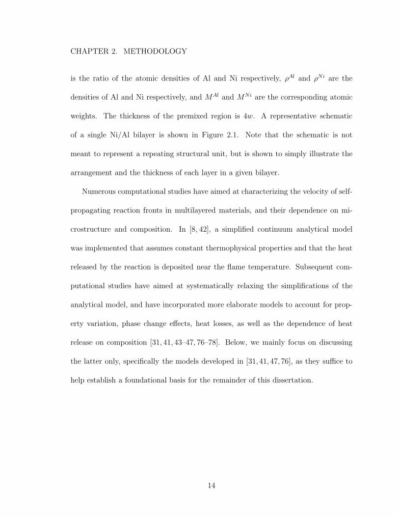
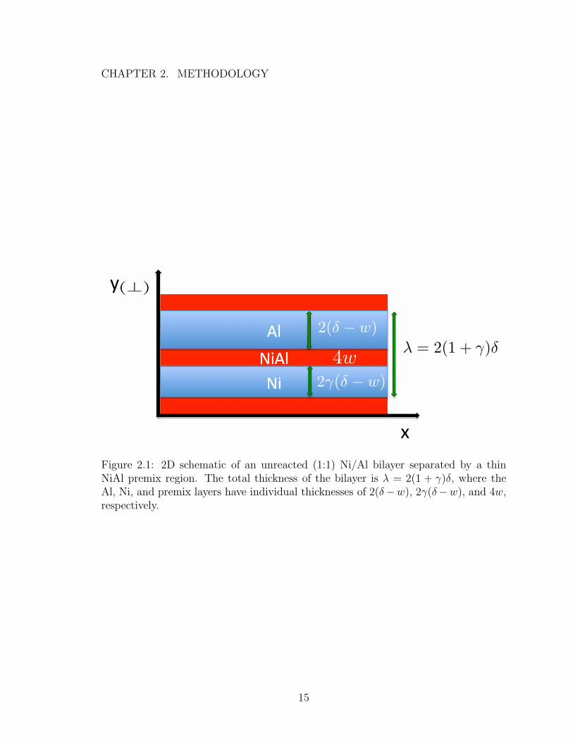
weights. The thickness of the premixed region is 4w. A representative schematic
of a single Ni/Al bilayer is shown in Figure 2.1. Note that the schematic is not
meant to represent a repeating structural unit, but is shown to simply illustrate the
arrangement and the thickness of each layer in a given bilayer.
Numerous computational studies have aimed at characterizing the velocity of self-
propagating reaction fronts in multilayered materials, and their dependence on mi-
crostructure and composition. In [8, 42], a simplified continuum analytical model
was implemented that assumes constant thermophysical properties and that the heat
released by the reaction is deposited near the flame temperature. Subsequent com-
putational studies have aimed at systematically relaxing the simplifications of the
analytical model, and have incorporated more elaborate models to account for prop-
erty variation, phase change effects, heat losses, as well as the dependence of heat
release on composition [31, 41, 43–47, 76–78]. Below, we mainly focus on discussing
the latter only, specifically the models developed in [31, 41, 47, 76], as they suffice to
help establish a foundational basis for the remainder of this dissertation.
14
CHAPTER 2. METHODOLOGY
!"
#"(⊥)
$%&'"
$%"
&'" 2(δ − w)
2γ(δ − w)
λ = 2(1 + γ)δ4w
Figure 2.1: 2D schematic of an unreacted (1:1) Ni/Al bilayer separated by a thinNiAl premix region. The total thickness of the bilayer is λ = 2(1 + γ)δ, where theAl, Ni, and premix layers have individual thicknesses of 2(δ−w), 2γ(δ−w), and 4w,respectively.
15

CHAPTER 2. METHODOLOGY
2.2 Continuum Model
Besnoin et al. [47] developed a continuum model for the multilayered system out-
lined in section 2.1, where the processes of atomic mixing and heat release in the
multilayer are described in terms of a coupled system of partial differential equations
expressing the evolution of a conserved scalar and enthalpy fields:
∂C
∂t= ∇ · (D(T )∇C) , (2.1)
ρ∂h
∂t= −∇ · q +
∂Q
∂t. (2.2)
The dimensionless conserved scalar, C, hereafter referred to as “concentration”, quan-
tifies the degree of atomic mixing; it varies between −1 ≤ C ≤ 1, and is defined such
that C = 1 is pure Al, C = −1 is pure Ni, and C = 0 is pure NiAl. The atomic
diffusivity, D, is assumed to be symmetric (i.e. does not depend on atomic iden-
tity), independent of concentration, and obeys a single Arrhenius law in the entire
temperature range characterizing the reaction, namely according to:
D(T ) = D0 exp
(
− Ea
RT
)
(2.3)
where T is temperature, R is the universal gas constant, D0 = 2.18 × 10⁻⁶ m2/s is
the pre-exponent, and Ea = 137 kJ/mol is the activation energy. The values of D0
and Ea are obtained as best fits based on experimental measurements of the velocity
of axially-propagating fronts [42].
It is important to note that Eq. (2.1) implicitly assumes that the reaction is
diffusion-limited, or in other words, that the time it takes for the reactants to react
16

CHAPTER 2. METHODOLOGY
upon encounter and form the product is almost instantaneous when compared to the
time it takes them to first diffuse towards each other.
In Eq. (2.2), h denotes the specific enthalpy, ρ is the mean density, and q is the
conductive heat flux given by Fourier’s law. Q is the heat released by the reaction
and is assumed to exhibit a quadratic dependence on concentration [43, 47]:
Q(C) = −∆HrxnC2 (2.4)
where ∆Hrxn is the (negatively signed) change of enthalpy (reaction enthalpy).
By making the additional assumptions that (i) the thermal conductivity, κ, is
isotropic and independent of temperature, and (ii) exploiting the separation of length
and time scales over which atomic and thermal diffusion occur2, Eq. (2.2) is further
simplified to (over a single bilayer for a 2-D system):
∂H
∂t= κ
∂2T
∂x2+
∂Q
∂t(2.5)
where κ is a constant mean thermal conductivity of the reactants, H is the layer-
averaged enthalpy,
∂Q
∂t= −ρcp∆Tf
∂C2
∂t, (2.6)
ρcp is the mean heat capacity per unit volume, ∆Tf is the temperature increase due
the reaction enthalpy, and
C2 =1
δ
∫ δ
0
C2(x, y, t)dy . (2.7)
2The thermal diffusivity is typically several orders of magnitude larger than the atomic diffusivity,which consequently makes the thermal front thickness (on the order of microns) also several orderof magnitude larger than the length scales over which atomic diffusion occurs (on the order ofnanometers). Thus, the temperature across a single bilayer can safely be assumed to be homogeneous.
17
CHAPTER 2. METHODOLOGY
Note that in defining the layer averages in Eqs. (2.6)–(2.7), the domain of interest
has been restricted to half the thickness of an Al layer, where y = δ coincides with
the centerline of the Al layer. This simplification exploits the symmetry of the flat,
periodic arrangement of the multilayer.
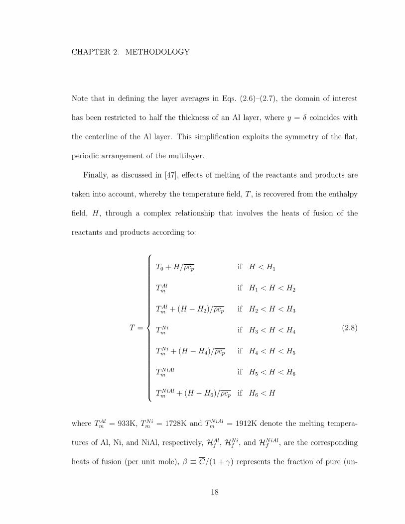
Finally, as discussed in [47], effects of melting of the reactants and products are
taken into account, whereby the temperature field, T , is recovered from the enthalpy
field, H , through a complex relationship that involves the heats of fusion of the
reactants and products according to:
T =
T0 +H/ρcp if H < H1
TAlm if H1 < H < H2
TAlm + (H −H2)/ρcp if H2 < H < H3
TNim if H3 < H < H4
TNim + (H −H4)/ρcp if H4 < H < H5
TNiAlm if H5 < H < H6
TNiAlm + (H −H6)/ρcp if H6 < H
(2.8)
where TAlm = 933K, TNi
m = 1728K and TNiAlm = 1912K denote the melting tempera-
tures of Al, Ni, and NiAl, respectively, HAlf , HNi
f , and HNiAlf , are the corresponding
heats of fusion (per unit mole), β ≡ C/(1 + γ) represents the fraction of pure (un-
18
CHAPTER 2. METHODOLOGY
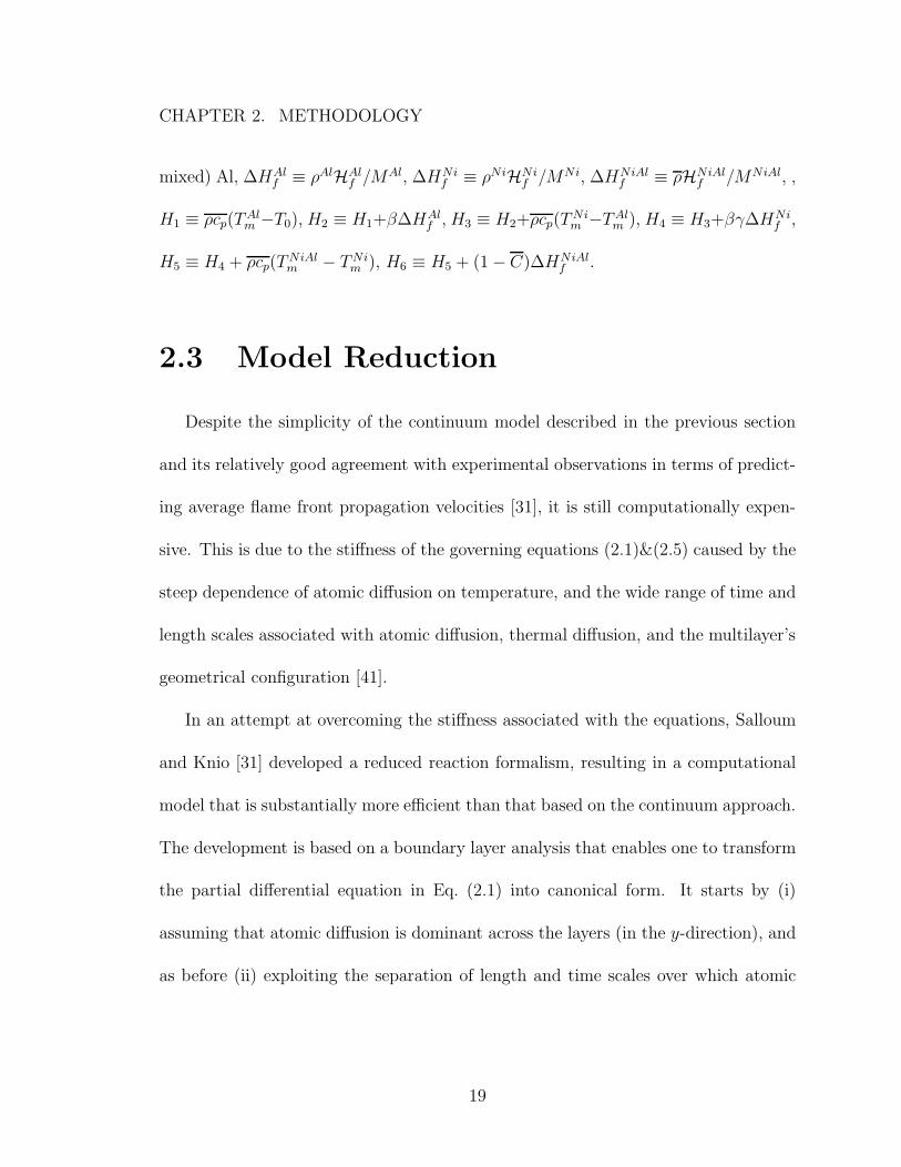
mixed) Al, ∆HAlf ≡ ρAlHAl
f /MAl, ∆HNif ≡ ρNiHNi
f /MNi, ∆HNiAlf ≡ ρHNiAl
f /MNiAl, ,
H1 ≡ ρcp(TAlm −T0),H2 ≡ H1+β∆HAl
f ,H3 ≡ H2+ρcp(TNim −TAl
m ),H4 ≡ H3+βγ∆HNif ,
H5 ≡ H4 + ρcp(TNiAlm − TNi
m ), H6 ≡ H5 + (1− C)∆HNiAlf .
2.3 Model Reduction
Despite the simplicity of the continuum model described in the previous section
and its relatively good agreement with experimental observations in terms of predict-
ing average flame front propagation velocities [31], it is still computationally expen-
sive. This is due to the stiffness of the governing equations (2.1)&(2.5) caused by the
steep dependence of atomic diffusion on temperature, and the wide range of time and
length scales associated with atomic diffusion, thermal diffusion, and the multilayer’s
geometrical configuration [41].
In an attempt at overcoming the stiffness associated with the equations, Salloum
and Knio [31] developed a reduced reaction formalism, resulting in a computational
model that is substantially more efficient than that based on the continuum approach.
The development is based on a boundary layer analysis that enables one to transform
the partial differential equation in Eq. (2.1) into canonical form. It starts by (i)
assuming that atomic diffusion is dominant across the layers (in the y-direction), and
as before (ii) exploiting the separation of length and time scales over which atomic
19
CHAPTER 2. METHODOLOGY
and thermal diffusion occur, thus simplifying Eq. (2.1) into:
∂C
∂t= D(T )
∂2C
∂y2. (2.9)
This is followed by introducing a normalized “layer age,”
τ ≡∫ t
0
D(T )
δ2dt′, (2.10)
and a normalized spatial variable ξ ≡ y/δ, which allows Eq. (2.9) to be recast into
approximate canonical form:
∂C
∂τ=
∂2C
∂ξ2. (2.11)
Numerically integrating Eq. (2.11) allows us to directly extract C, and hence C and
C2, for a given value of τ . Moreover, using the same set of assumptions as be-
fore, the differential energy equation (2.2) can also be replaced with its volume- or
region-averaged form. Consequently, the resulting system of equations governing the
evolution of the reaction is expressed as:
∂τ
∂t=
D(T )
δ2(2.12)
∂H
∂t= − 1
V
∫
V
(∇ · q)dV +∂Q
∂t(2.13)
where H is the volume-averaged enthalpy, V is the volume of a computational cell
or region3 which is taken to be fixed and semi-closed (admits heat but not mass
3The volume of the cell in this case, or the area in the case of the layer-averaged formulation
20
CHAPTER 2. METHODOLOGY
diffusion),
∂Q
∂t= −ρcp∆Tf
∂C2(t)
∂t(2.14)
is the volume-averaged heat release term, ρcp is the mean heat capacity per unit
volume, ∆Tf ≡ ∆Hrxn/ρcp is the temperature increase due the reaction enthalpy,
and
C2 =1
V
∫
V
C2dV . (2.15)
The dependence of C and C2 on τ can be expressed in terms of a canonical solu-
tion, which is tabulated in a pre-processing step and made available to the computa-
tions [31]. The temperature, T , can be recovered as before using the relationship in
Eq. (2.8) .
According to the formulation outlined above, we can see that the advantages of
the reduced model over the detailed model are that it (1) eliminates the need of
using a fine scale mesh in order to resolve the process of atomic mixing occurring
at the nano-scales through replacing the evolution equation for C with an evolution
equation for τ , and (2) requires the computation of only global (average) spatial and
temporal reaction and thermal diffusion terms, thus reducing the stiffness inherent
in the governing equations of the detailed model and allowing for substantially larger
integration time-steps (this is true even when semi-implicit integration schemes are
used in the detailed model as in [45–47]).
discussed in the previous section, is defined such that largest dimension is ≪ the thermal frontthickness in order to ensure the validity of the temperature homogeneity assumption. Later on, asystematic mesh refinement study will be conducted in order to determine a suitable mesh size thatwould satisfy this requirement.
21
CHAPTER 2. METHODOLOGY
To check the validity of the reduced model and quantify the enhancement in com-
putational efficiency that it offered, Salloum and Knio [31, 41, 76] conducted various
numerical experiments comparing the results of both, the reduced and the detailed
models. The analysis indicated that the two models gave predictions of average ve-
locities of self-propagating fronts and ignition thresholds that were in agreement, and
that the required CPU time using the reduced model was up to 64 times less than
that needed by the detailed model. Moreover, they demonstrated the capability of
extending the reduced formalism to include transient multidimensional computations
in both uniform and heterogeneous multilayers — a feature that would have been
prohibitively expensive using the detailed model.
Having been tested and validated, the reduced continuum methodology will be
adopted as our starting point for the remainder of this thesis. In what follows, a brief
description of the numerical scheme (adapted from [41]) utilized for implementing the
reduced model is provided.
2.4 Numerical Scheme
The reduced model outlined in section 2.3 involves a coupled system of equations,
(2.12) and (2.13). Numerical solution of this system of equations is conducted using
a finite-difference scheme that is adapted from [41, 76]. Brief details are provided
below.
22

CHAPTER 2. METHODOLOGY
For simplicity, we focus on simple domains, rectangles in 2D or boxes in 3D, which
are discretized using a uniform grid. The cell sizes in the x, y and z direction are
denoted by ∆x, ∆y and ∆z, respectively. Field variables are discretized on cell cen-
ters, whereas fluxes are defined at cell edges. Consequently, with each computational
cell one associates the discrete state vector, (H, τ ), composed of the enthalpy, H ,
and the local age of the individual subregions contained in the computational cell, τp,
p = 1, . . . , N (where N denotes the number of subregions4). All other local physical
quantities can be readily obtained based on the local state vector. In particular, the
temperature, T , can be retrieved from the volume-averaged enthalpy, H , by inverting
a complex relationship involving the heats of fusion of the constituents (Eq. (2.8)) [76].
A second-order, conservative, centered-difference approximation is used to esti-
mate the conduction heat fluxes at the faces of each computational cell. This ap-
proximation transforms the governing equations (2.12) and (2.13) into a discrete
system of coupled ODEs. The resulting discrete system is advanced in time using
the mixed scheme introduced in [41]. This scheme combines exact treatment of the
source term appearing on the right-hand side of (2.13), with Runge-Kutta-Chebychev
(RKC) [79–83] treatment of the thermal and atomic diffusion terms. Additional de-
tails regarding the construction of the mixed integration scheme can be found in [41].
In all the 1D and 2D computations discussed in the subsequent chapters, adiabatic
conditions are imposed on all domain boundaries (unless otherwise noted). In these
4A region is defined as a subset of the computational domain whose dimensions are ≪ than thethermal front width, and a subregion is a subset of this region which has a uniform δ layering. Aregion could be comprised of one or more subregions.
23

CHAPTER 2. METHODOLOGY
computations, ignition is simulated by imposing an initial temperature profile within
the domain such that T (x, t = 0) = Ts for 0 ≤ x ≤ ws, where Ts and ws are the
spark temperature and width respectively. Beyond the spark region, the temperature
decreases linearly to the ambient temperature, T0, according to:
T (x, t = 0) = T0 + (Ts − T0)(2ws − x)/ws for ws ≤ x ≤ 2ws,
T (x, t = 0) = T0 for x ≥ 2ws
In the 3D computations, ignition is simulated by imposing a surface heat flux on
a portion of the domain boundary, which is maintained constant over a fixed time
period. At all other times, and all other locations, adiabatic boundary conditions are
used, as in the 1D and 2D computations.
As discussed in [76], the thin premix region is accounted for by setting the initial
value of the average composition to C(t = 0) = 1 − w/δ. In all the cases considered
(unless otherwise noted), a constant premix width w = 0.8 nm was prescribed, and
the computations are performed using a uniform Cartesian grid. Accordingly, for
δ > 12 nm, a cell size ∆x = ∆y = ∆z = 1 µm was used, whereas ∆x = ∆y =
∆z = 0.5 µm for smaller values of δ. These mesh resolutions were selected following
a systematic mesh refinement analysis that aimed to ensure that the predicted front
properties became essentially independent of cell size.
24

Chapter 3
Effects of Thermal Diffusion
3.1 Motivation
It is now well known that the average velocity of the front depends on a number
of factors [8, 23, 29, 42–48], including ambient conditions, layer thickness, material
composition, and on the microstructure or uniformity of the layering. The dynamics
of self-propagating fronts in multilayers can however be complex under certain condi-
tions, even when the layering (or microstructure) is essentially uniform. For instance,
evidence of oscillatory front motion has been predicted computationally [45,47] as well
as seen experimentally [84]. Recently, it has also been observed that self-propagating
fronts in multilayers can exhibit cellular [49], or spinlike features [85]. These transient
front dynamics can thus be inherently multidimensional in nature.
In addition to enabling simulations in two and three space dimensions, the reduced
25
CHAPTER 3. EFFECTS OF THERMAL DIFFUSION
reaction methodology developed in [31,41,76] has shown that by using this formalism
one is able to predict the behavior of multilayer composites that feature non-uniform
layering, particularly when the front behavior cannot be readily described using an
average layering [29, 76].
To reproduce the front velocity in nonuniform multilayers, a variable thermal
conductivity model was developed in [76] which accounts for the dependence of the
thermal conductivity on the local concentration, but otherwise ignores potential tem-
perature and directional effects. The effects of property variation with temperature
and concentration were in fact considered in the analysis of Gunduz et al. [86]. How-
ever, this analysis assumed that physical properties were isotropic, and was restricted
to quasi-1D axial front propagation. Consequently, the impact of the dependence of
thermal conductivity on concentration, temperature, and material layering is as of
yet not well understood. The present study addresses this issue, through a systematic
analysis of various thermal conductivity models.
To this end, we consider four different thermal conductivity models. The first
is a constant conductivity model, where following [45] the thermal conductivity is
approximated by the average conductivity of the reactants and taken to be fixed in
space and time. The second model is the concentration dependent thermal conduc-
tivity model developed in [76]. In this model, the thermal conductivity is treated as
isotropic, temperature effects are ignored, but the dependence on local composition
is directly accounted for using a simplified mixture rule. The third model generalizes
26

CHAPTER 3. EFFECTS OF THERMAL DIFFUSION
the second by accounting for the impact of the reactants’ layering. It is motivated
by experimental observations of nanostructured multilayers [87] which indicate that
the in-plane thermal diffusivity may be several orders of magnitude larger than the
normal (i.e. perpendicular to the layers) thermal diffusivity. Finally, the fourth model
generalizes the third by accounting for the temperature dependence of the individual
constituents.
In order to illustrate the role and ramifications each of these dependencies has on
the flame dynamics, we contrast predictions obtained using the four models on the
average front velocity in nanostructured Ni/Al multilayers. In doing so, the bilayer
thickness is systematically varied. Furthermore, we also contrast the results obtained
for Ni/Al and NiV/Al multilayered systems (V stands for Vanadium) in order to
briefly explore whether the substantial difference in the thermal conductivity of pure
Ni and relevant Ni alloys1 would lead to a substantial difference in reaction front
velocities.
In addition to analyzing the behavior of flame velocities, a systematic study is
conducted of the quasi-1D structure of the reaction front. This effort is motivated by
the fact that despite the availability of various studies focusing on self-propagating re-
actions in nanolaminates, several relevant features of the reaction front have not been
thoroughly investigated, including the dependence of thermal and reaction widths on
the bilayer thickness, as well as the variation of the composition with temperature.
1The NiV/Al multilayers are fabricated by vapor deposition using pure Al and NiV (7% wt V)targets [29]. Unlike pure Ni, the Ni93V7 alloy is non-magnetic, which offers advantages during thedeposition process.
27

CHAPTER 3. EFFECTS OF THERMAL DIFFUSION
Investigation of these features is further motivated by the development of advanced
diagnostic tools [38, 49] which are enabling direct observations into the front struc-
ture, as well as molecular simulations [88–91] which offer the possibility of developing
more elaborate reaction models. Specifically, a detailed characterization of the quasi-
1D front structure would be helpful for the purpose of planning measurements or
multiscale computations, and ultimately for validating or refining reduced models.
Finally, results from a limited number of 3D computations are outlined. These
are used to conduct a preliminary exploration of the role of the thermal model on
transient front motion in three dimensions.
3.2 Derivation of the generalized thermal
transport models
Our goal in this chapter is to study the effect of thermal diffusion on the dy-
namics of the flame propagation, and specifically on the role played by the thermal
conductivity. In all cases, the heat flux q is assumed to follow Fourier’s law, namely
q = −κ∇T (3.1)
where κ is the thermal conductivity. As mentioned above, new models are developed
in the present study that account for the effects of material heterogeneity (layering)
and the variation of thermal conductivity with temperature. Results obtained with
28

CHAPTER 3. EFFECTS OF THERMAL DIFFUSION
these new models are contrasted with predictions obtained based on earlier, simpler
models, namely those corresponding to a constant conductivity [47], or to an isotropic,
concentration-dependent conductivity [76]. For the sake of completeness, all models
considered in the present work are outlined below.
3.2.1 Constant κ
Original models of self-propagating reactions in reactive nanolaminates [42, 44,
45, 92, 93] have relied on a constant conductivity approximation. Presently, this is
implemented using an appropriate average conductivity of the reactants. For a Ni/Al
system, with a 1:1 ratio of the reactants, the thermal conductivity is expressed as:
κ = κ ≡ κAl + γκNi
1 + γ(3.2)
where κAl = 237 Wm−1K−1and κNi = 91 Wm−1K−1refer to the room-temperature
thermal conductivities of Al and Ni, respectively. (These estimates are discussed in
section 3.2.4). In the computations below, we shall also consider a variant of (3.2)
adapted to an NiV/Al system. In the latter case, the thermal conductivity is given
by:
κ = κ ≡ κAl + γκNiV
1 + γ(3.3)
where κNiV = 18.9 Wm−1K−1is the thermal conductivity of Ni(93%)V(7%) at room
temperature, see section 3.2.4.
29
CHAPTER 3. EFFECTS OF THERMAL DIFFUSION
3.2.2 Concentration dependent κ
In [76], an isotropic, concentration-dependent thermal conductivity model was
developed. The model considered Ni/Al multilayers, and the thermal conductivity
was expressed as:
κ = (κ− κNiAl)C + κNiAl (3.4)
where κ is given by (3.2) and κNiAl = 92 Wm−1K−1is the room temperature thermal
conductivity of NiAl, see section 3.2.4.
For NiV/Al multilayers, the mixture-based approach in [76] yields:
κ = (κ− κNiV Al)C + κNiV Al (3.5)
where κ is given by (3.3) and κNiV Al = 48.7 Wm−1K−1is the room temperature
thermal conductivity of NiVAl, see section 3.2.4. In the computations below, we
contrast results obtained for the different multilayer compositions using the κ models
given by (3.2)–(3.5), as well as more elaborate models developed below.
3.2.3 Direction-dependent κ
This section extends the concentration-dependent conductivity formulation above
by accounting for the anisotropy of the unreacted medium. Specifically, due to the
initial layering of the nanolaminate, and the differences in the thermal conductivities
of individual layers, transport rates may generally differ according to whether the
temperature gradient is parallel to the layers, or normal to the layers. This may po-
30
CHAPTER 3. EFFECTS OF THERMAL DIFFUSION
tentially affect the motion of the self-propagating front, particularly when propagation
occurs along multiple space dimensions, or normal to the layering [41].
As shown in Fig. 2.1, the total thickness of the bilayer (including the premix) is λ,
the Al layer has a thickness tAl = αλC, and the Ni layer has a thickness tNi = βλC,
where α and β represent the fractional thickness volumes of Ni and Al, respectively.
For nanolaminates with a 1:1 Ni/Al composition, we have:
α ≡ 1
1 + γ,
and
β ≡ γ
1 + γ.
The anisotropic character of κ will be assumed to be solely the result of the layered
configuration of the system. Thus, the direction-dependent κ matrix will be diagonal,
of the form:
κ =
κ‖ 0 0
0 κ⊥ 0
0 0 κ‖
where κ‖ designates the in-plane (x and z directions) conductivity, and κ⊥ designates
the thermal conductivity along the normal (y) direction.
For brevity, we focus our attention on Ni/Al nanolaminates and seek expressions
for κ‖ and κ⊥ by considering two scenarios, namely one in which heat is flowing along
the layers, and another where heat is flowing normal to the layers. The former case
31

CHAPTER 3. EFFECTS OF THERMAL DIFFUSION
is analogous to the situation of an electric circuit with resistors connected in parallel,
whereas the second corresponds to resistors connected in series. Accordingly, κ‖ can
expressed as the weighted sum of the individual thermal conductivities for Al, Ni,
and NiAl, according to:
κ‖ =κAltAl + κNitNi + κNiAltNiAl
λ.
Substituting the appropriate expressions for the individual layer thicknesses conse-
quently yields:
κ‖ = ακAlC + βκNiC + κNiAl(1− C) . (3.6)
When heat flows normal to the layering, continuity of the normal flux immediately
yields:
κNi∆TNi
tNi
= κ⊥∆Tλ
κAl∆TAl
tAl
= κ⊥∆Tλ
κNiAl∆TNiAl
tAl
= κ⊥∆Tλ
where ∆TNi, ∆TAl, ∆TNiAl, are the temperature differences across the Ni, Al, and
NiAl layers, respectively, and ∆T = ∆TNi + ∆TAl + ∆TNiAl is the overall tempera-
ture drop across the corresponding bilayer. Summing the above three equations and
substituting for the individual layer thicknesses, we get:
1
κ⊥=
βC
κNi
+αC
κAl
+1− C
κNiAl
(3.7)
32
CHAPTER 3. EFFECTS OF THERMAL DIFFUSION
The analysis above can be repeated for nanolaminates comprised of NiV/Al mul-
tilayers and one obtains:
κ‖ = ακAlC + βκNiVC + κNiV Al(1− C) , (3.8)
and
1
κ⊥=
βC
κNiV
+αC
κAl
+1− C
κNiV Al
. (3.9)
3.2.4 Direction and temperature dependent κ
It is well known [94–98] that the thermal conductivity may exhibit a strong de-
pendence on temperature. Consequently, we construct an extension of the direction-
dependent model of the previous section, namely by accounting for the variation of
the conductivity with temperature. The extension essentially consists in estimating
the temperature dependence of the individual conductivities appearing in (3.6–3.9),
namely Al, Ni, NiAl, Ni(93%)V(7%), and Ni(46.5%)V(3.5%) Al(50%). Below, we
seek correlations that approximate the corresponding conductivity values in a wide
temperature range that includes temperatures typically encountered in reacting front
computations, 298K ≤ T ≤ 2500K.
Temperature dependence of κAl
A comprehensive database for pure Al at temperatures both above and below the
melting point has been gathered from previous studies and scrutinized both empiri-
33
CHAPTER 3. EFFECTS OF THERMAL DIFFUSION
cally and theoretically by Touloukian et al. [99], who provide a table of recommended
thermal conductivity values. Expressions of κAl(T ) were obtained from best fits to
these recommended values. Since the thermal conductivity of Al exhibits a disconti-
nuity at the melting temperature, two separate fits had to be determined, one for the
solid state and another for the liquid state. Figure 3.1 depicts the data of Touloukian
et al. [99], within the temperature range of interest, along with the best fits for the
solid and liquid states, respectively:
κAl(solid)(T ) = aT 6 + bT 5 + cT 4 + dT 3 + eT 2 + fT + g T < Tm
κAl(liquid)(T ) = a′
T 4 + b′
T 3 + c′
T 2 + d′
T + e′
T ≥ Tm
(3.10)
where κ is in Wm−1K−1, Tm ≈ 933K, a ≈ 1.0496 × 10⁻¹⁴, b ≈ −3.7969 × 10⁻¹¹,
c ≈ 5.5101 × 10⁻⁸, d ≈ −4.0679 × 10⁻⁵, e ≈ 0.015847,f ≈ −3.0421, g ≈ 460.18,
a′ ≈ −1.0232 × 10⁻¹³, b
′ ≈ 2.4885 × 10⁻⁹, c′ ≈ −2.287 × 10⁻⁵, and d
′ ≈ 0.073068,
and e′ ≈ 40.758.
Remark: Practical manufacturing processes can utilize high purity Al targets, or Al
alloy targets such as Al(1100) [95,99]. However, the amount of dopants or impurities
in the Al alloy targets is generally very small, and the thermal conductivity of de-
posited Al layers is expected to remain fairly close to that of pure Al. Consequently,
in the analysis below, we ignore potential effects of impurities or diluents on thermal
conductivity of Al, and consider exclusively the pure Al estimate (3.10) above.
34

CHAPTER 3. EFFECTS OF THERMAL DIFFUSION
200 500 1000 1500 2000 260080
100
120
140
160
180
200
220
240
260
Temperature (K)
Th
erm
al C
on
du
ctivity (
W/m
/K)
Touloukien data
Fit
Melting Temp.
Al
Figure 3.1: Thermal conductivity of pure Al as a function of temperature. Shown aredata from Touloukian et al. [99], along with the two best fits for the solid and liquidstates of Al. The melting temperature indicated in the plot is 933K approximately;R2 ≈ 0.9992 for the fit in the solid state, whereas R2 ≈ 0.9998 for the one in theliquid state region.
35
CHAPTER 3. EFFECTS OF THERMAL DIFFUSION
Temperature dependence of κNi and κNiV
Thermal conductivity values for pure Ni as a function of temperature were ob-
tained from [94]. The value of κNi at the Curie temperature, which was not given
in [94], was adapted from [99]. A best fit to the resulting data set was obtained, and
used to construct a suitable expression for κNi(T ). Two separate branches were estab-
lished in order to correctly capture the behavior of κNi(T ) below and above the Curie
temperature. The best fit for κNi(T ) below the Curie temperature, TC = 631K, is a
3rd order polynomial, while that for temperatures above TC is linear:
κNi(T ) = aT 3 + bT 2 + cT + d T < TC
κNi(T ) = a′
T + b′
T ≥ TC
(3.11)
where κ is in Wm−1K−1, a ≈ −3.4997 × 10⁻⁷, b ≈ 5.7741 × 10⁻⁴, c ≈ −0.38236,
d ≈ 162.93, a′ ≈ 0.021563, and b
′ ≈ 50.2632. The original data along with the
fits are shown in Fig. 3.2. Note that available experimental data for the thermal
conductivity of Ni does not extend beyond the Ni melting temperature, TNim = 1728K.
Consequently, the correlation (3.11) for κNi(T ), T ≥ TC , has simply been extrapolated
to temperatures exceeding the Ni melting temperature.
In contrast to pure Ni, experimental values of the thermal conductivity of Ni(93%)V(7%)
are generally lacking. Consequently, an approximate κNiV (T ) relationship was con-
structed, as outlined below.
36
CHAPTER 3. EFFECTS OF THERMAL DIFFUSION
200 500 1000 1500 2000 260060
65
70
75
80
85
90
95
100
105
110
Temperature (K)
Th
erm
al C
on
du
ctivity (
W/m
/K)
CRC data
Fit
Curie Temp.
Ni!Pure
Figure 3.2: Thermal conductivity of pure Ni as a function of temperature. Shownare the original data reported in [94] along with the best two fits for the data belowand above the Ni Curie temperature, TC ≈ 631K. The value of κNi at TC has beenobtained from [99]. R2 ≈ 0.9997 for T < TC , whereas R
2 ≈ 0.9999 for T ≥ TC .
37

CHAPTER 3. EFFECTS OF THERMAL DIFFUSION
We start by estimating the thermal conductivity of NiV at room temperature. To
this end, we rely on measured values of the thermal conductivity at room temperature
of the NiV/Al multilayers in the normal direction; these range between 35 and 50
Wm−1K−1 [100]. Using (3.9), taking k⊥ to be the mean of the reported experimental
range (≈ 42.5Wm−1K−1), substituting for the corresponding value of κAl(298K) ≈
237.05Wm−1K−1, and neglecting the contribution of the thin NiVAl premix region i.e.
setting C = 1, one deduces an approximate value for κNiV (298K) ≈ 18.93 Wm−1K−1.
Using the room temperature value above, an approximate κNiV (T ) is then con-
structed by assuming that the temperature dependence of the thermal conductivity
of NiV is similar to that of pure Ni above the Curie temperature. This results in:
κNiV (T ) = aT + b [Wm−1K−1] (3.12)
where a ≈ 0.021563, and b ≈ 12.5072. This approximation appears to be reasonable
because the Curie temperature of Ni(93%)V(7%) is lower than 298K [101–103]. An
additional rationalization is based on the observation that the thermal conductivity
of Ni(90%)Cr(10%) exhibits a linear dependence on temperature with a slope close
to that of pure Ni [99] above TC .
Temperature dependence of κNiAl and κNiV Al
Relationships for κNiAl(T ) and κNiV Al(T ) were constructed based on an experi-
mental study of Terada et al. [97], which reports measurements on the variation of
thermal conductivity with temperature for different NiAl alloys. (See Fig. 5 in [97].)
38
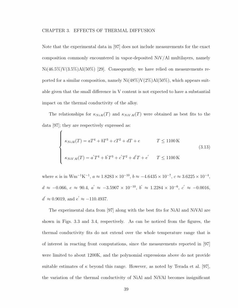
CHAPTER 3. EFFECTS OF THERMAL DIFFUSION
Note that the experimental data in [97] does not include measurements for the exact
composition commonly encountered in vapor-deposited NiV/Al multilayers, namely
Ni(46.5%)V(3.5%)Al(50%) [29]. Consequently, we have relied on measurements re-
ported for a similar composition, namely Ni(48%)V(2%)Al(50%), which appears suit-
able given that the small difference in V content is not expected to have a substantial
impact on the thermal conductivity of the alloy.
The relationships for κNiAl(T ) and κNiV Al(T ) were obtained as best fits to the
data [97]; they are respectively expressed as:
κNiAl(T ) = aT 4 + bT 3 + cT 2 + dT + e T ≤ 1100K
κNiV Al(T ) = a′
T 4 + b′
T 3 + c′
T 2 + d′
T + e′
T ≤ 1100K
(3.13)
where κ is in Wm−1K−1, a ≈ 1.8283× 10⁻¹⁰, b ≈ −4.6435× 10⁻⁷, c ≈ 3.6225× 10⁻⁴,
d ≈ −0.066, e ≈ 90.4, a′ ≈ −3.5907 × 10⁻¹⁰, b
′ ≈ 1.2284 × 10⁻⁶, c′ ≈ −0.0016,
d′ ≈ 0.9019, and e
′ ≈ −110.4937.
The experimental data from [97] along with the best fits for NiAl and NiVAl are
shown in Figs. 3.3 and 3.4, respectively. As can be noticed from the figures, the
thermal conductivity fits do not extend over the whole temperature range that is
of interest in reacting front computations, since the measurements reported in [97]
were limited to about 1200K, and the polynomial expressions above do not provide
suitable estimates of κ beyond this range. However, as noted by Terada et al. [97],
the variation of the thermal conductivity of NiAl and NiVAl becomes insignificant
39

CHAPTER 3. EFFECTS OF THERMAL DIFFUSION
at high temperatures. Therefore, the correlations reported in (3.13) are limited to
T ≤ 1100 K, and the thermal conductivities of κNiAl and κNiV Al for T > 1100 K, are
approximated by the corresponding values at T = 1100 K.
Remark: As for Ni, available experimental measurements of the thermal conductivities
of NiAl and NiVAl do not extend above the corresponding melting temperatures.
Potential variations in κ at or above the melting temperature have consequently been
ignored.
Summary
Having obtained the necessary expressions of κ(T ) for the various compounds,
one can incorporate the effects of direction and temperature dependence simply by
substituting these expressions into(3.6)–(3.9). Figure 3.5 shows the estimated values
of the thermal conductivity in Ni/Al multilayers, whereas Fig. 3.6 shows estimated κ
values for NiV/Al multilayers. In both cases, the estimate corresponding to a constant
thermal conductivity approximation is also depicted.
40

CHAPTER 3. EFFECTS OF THERMAL DIFFUSION
200 300 400 500 600 700 800 900 1000 1100 120088
90
92
94
96
98
100
102
104
106
108
Temperature (K)
Th
erm
al C
on
du
ctivity (
W/m
/K)
Terada data
Fit
NiAl
Figure 3.3: Thermal conductivity of stoichiometric NiAl as a function of temperature.Shown are the data reported by Terada et al. [97] along with the best fit for the data.R2 ≈ 0.9955.
41

CHAPTER 3. EFFECTS OF THERMAL DIFFUSION
200 300 400 500 600 700 800 900 1000 110010
20
30
40
50
60
70
80
90
100
Temperature (K)
Therm
al C
onductivity (
W/m
/K)
Terada data
Fit
NiVAl
Figure 3.4: Thermal conductivity of Ni(48%)V(2%)Al(50%) as a function of temper-ature. Shown are the data reported by Terada et al. [97] along with the best fit forthe data. R2 ≈ 0.9993.
42
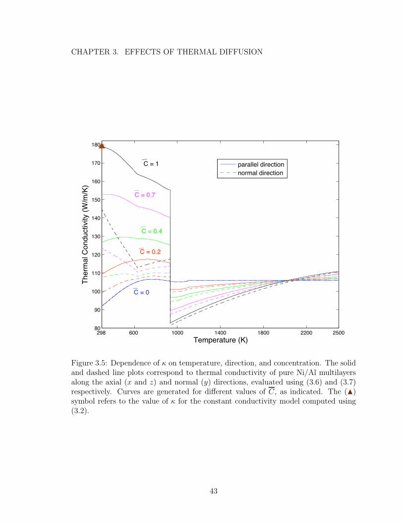
CHAPTER 3. EFFECTS OF THERMAL DIFFUSION
298 600 1000 1400 1800 2200 250080
90
100
110
120
130
140
150
160
170
180
Temperature (K)
Therm
al C
onductivity (
W/m
/K)
parallel direction
normal direction
C = 0
C = 0.4
C = 1
C = 0.2
C = 0.7
Figure 3.5: Dependence of κ on temperature, direction, and concentration. The solidand dashed line plots correspond to thermal conductivity of pure Ni/Al multilayersalong the axial (x and z) and normal (y) directions, evaluated using (3.6) and (3.7)respectively. Curves are generated for different values of C, as indicated. The (N)symbol refers to the value of κ for the constant conductivity model computed using(3.2).
43

CHAPTER 3. EFFECTS OF THERMAL DIFFUSION
298 600 1000 1400 1800 2200 250040
60
80
100
120
140
160
Temperature (K)
Therm
al C
onductivity (
W/m
/K)
parallel direction
normal direction
C = 0.4
C = 0.2
C = 0
C = 0.7
C = 1
Figure 3.6: Dependence of κ on temperature, direction, and concentration. Thesolid and dashed line plots correspond to thermal conductivity of NiV/Al multilayersalong the axial (x and z) and normal (y) directions, evaluated using (3.8) and (3.9)respectively. Curves are generated for different values of C, as indicated. The (N)symbol refers to the value of κ for the constant conductivity model, computed using(3.3).
44
CHAPTER 3. EFFECTS OF THERMAL DIFFUSION
3.3 Results
In this section, we provide a comparative analysis of results obtained using the
different thermal conductivity models outlined above, for both Ni/Al and NiV/Al
multilayers. We base our analysis on three main characteristics of the flame front,
namely (i) the average thermal width, (ii) the average reaction width, and (iii) the
average axial velocity. We start first by defining each of these three properties and
the means by which they are calculated. We then move on to presenting results of
the quasi-1D computations which involve comparing the constant, concentration de-
pendent, and concentration and temperature dependent conductivity models. This
analysis is then extended to normally-propagating fronts [41], based on performing
two sets of nominally 2D computations: one for a flame propagating along the layers
(x-direction), and another for a flame propagating normal to the layers (y-direction).
We restrict this to (i) the concentration and direction dependent, and (ii) concentra-
tion, direction and temperature dependent κ models, since the other two models do
not include direction dependence and are thus insensitive to propagation direction.
Finally, we present preliminary results from 3D computations using the direction and
temperature dependent κ models which show unsteady propagation dynamics that
are reminiscent of recent experimental observations [85, 104].
45
CHAPTER 3. EFFECTS OF THERMAL DIFFUSION
3.3.1 Front Properties
The structure of quasi-1D reaction fronts is characterized in terms of the thermal
and reaction widths. Letting x denote the propagation direction, the thermal width
of the front is defined in terms of the gradient of the temperature profile. Specifically,
the gradient profile is first computed, and the standard deviation, σT , of the resulting
profile is used as a measure of the thermal width. The procedure is based on first
defining the thermal mean, xT , according to:
xT =
∫
x∂T
∂xdx
∫
∂T
∂xdx
(3.14)
and then computing σT from:
σ2T =
∫
(x− xT )2∂T
∂xdx
∫
∂T
∂xdx
(3.15)
The reaction width is defined in a similar fashion. Specifically, we first compute the
reaction mean,
xR =
∫
x∂Q
∂tdx
∫
∂Q
∂tdx
(3.16)
where ∂Q/∂t is the local heat release term, and then deduce the reaction width, σR,
from:
σ2R =
∫
(x− xR)2∂Q
∂tdx
∫
∂Q
∂tdx
(3.17)
Since in some cases the front propagates in an unsteady fashion, in the results we re-
port averages (arithmetic means) taken at four separated time instants, corresponding
46

CHAPTER 3. EFFECTS OF THERMAL DIFFUSION
to flame positions that are appreciably away from the domain boundaries.
As discussed in [31], the average axial front velocity is simply deduced by fitting
a linear curve to (xR(t), t) data pairs.
3.3.2 Axial Front Structure
In this subsection, we focus on a quasi-1D geometry, and contrast predictions
obtained using three thermal conductivity models. The analysis covers a wide range
of bilayer thicknesses, specifically δ = 12, 24, 48, 72, 120, and 300 nm, and in addition,
contrasts results for Ni/Al and NiV/Al multilayers.
Figure 3.7 shows σT plotted against δ, for the constant, concentration dependent,
and temperature dependent κ-models. Shown are results for both Ni/Al multilay-
ers and NiV/Al multilayers. It can be noticed that for small bilayers, δ ≤ 48nm,
the predictions of the different models are very close to one another, but flare out
slightly as δ increases. In the range considered, the σT versus δ curves appear es-
sentially linear, and the predicted thermal widths for NiV/Al are consistently lower
than those for Ni/Al. This appears consistent with the observation that the overall
thermal conductivity values of the NiV/Al multilayers are smaller than those of Ni/Al
multilayers.
Figure 3.8 shows predicted values of σR plotted against δ. Shown are results
obtained using the constant, concentration dependent, and temperature dependent
κ-models, for both Ni/Al and NiV/Al multilayers. As for σT , the reaction width also
47
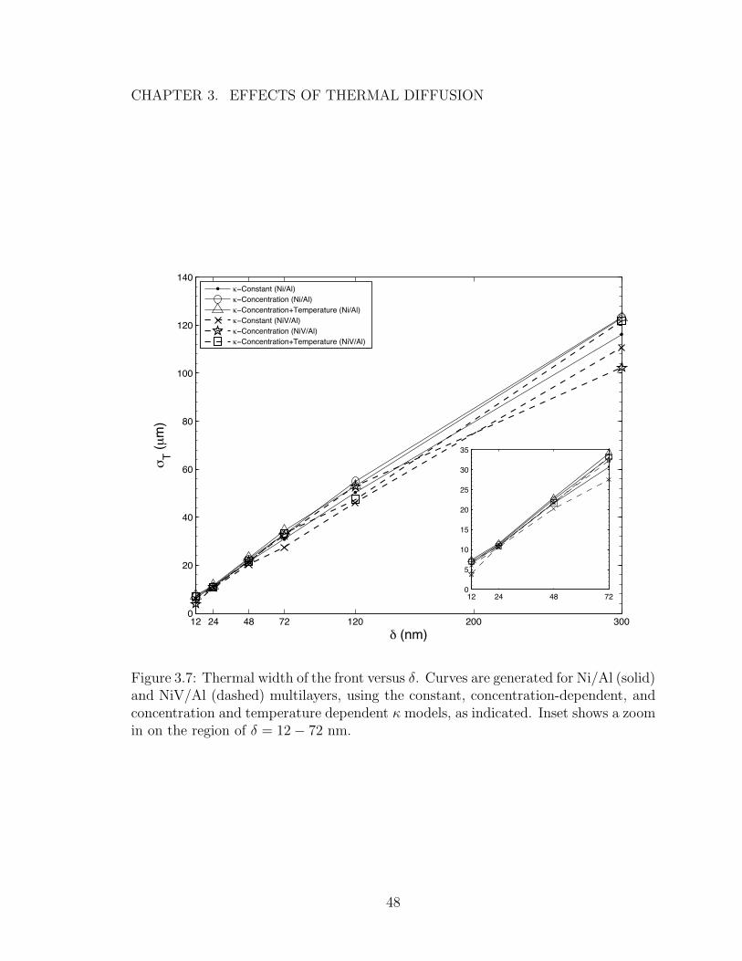
CHAPTER 3. EFFECTS OF THERMAL DIFFUSION
12 24 48 72 120 200 3000
20
40
60
80
100
120
140
! (nm)
"T (µ
m)
#!Constant (Ni/Al)
#!Concentration (Ni/Al)
#!Concentration+Temperature (Ni/Al)
#!Constant (NiV/Al)
#!Concentration (NiV/Al)
#!Concentration+Temperature (NiV/Al)
12 24 48 720
5
10
15
20
25
30
35
Figure 3.7: Thermal width of the front versus δ. Curves are generated for Ni/Al (solid)and NiV/Al (dashed) multilayers, using the constant, concentration-dependent, andconcentration and temperature dependent κ models, as indicated. Inset shows a zoomin on the region of δ = 12− 72 nm.
48
CHAPTER 3. EFFECTS OF THERMAL DIFFUSION
exhibits an essentially linear dependence on δ, and lower values of σR are predicted for
NiV/Al multilayers than for Ni/Al multilayers. In the present case, however, the re-
action widths for the temperature dependent κ-model appear to be smaller than those
for the constant and concentration dependent κ-models whose values are comparable.
In addition, differences between the outputs of the different models becomes apparent
at δ = 24 nm, i.e. at smaller bilayers than for σT . Absolute differences become more
pronounced as δ increases, though the ratio of σR for the constant κ-model to that
of the temperature dependent κ-model retains a constant value of approximately 1.4
throughout the range of δ’s considered. The same trend is observed for both the
Ni/Al and NiV/Al multilayers. It is also interesting to note that for NiV/Al multi-
layers having small bilayer thickness, the time resolved TEM measurements of Kim
et al. [49] reveal a very sharp concentration contrast. Specifically, for a 2:3 Al/NiV
multilayer with 25nm bilayers, the TEM micrographs suggest a transition between
unmixed and essentially mixed states on the order of microns. This appears to be
consistent with the σR predictions for the smallest values of δ considered.
Figure 3.9 shows the average axial flame velocity as a function of δ, on a log-
log scale, for the Ni/Al and NiV/Al multilayers using the same three κ-models. In
accordance with previous theoretical, numerical, and experimental observations [29,
31,41,42,76,93] in the present cases the average flame velocity decreases as δ increases.
This is expected since we have focused on a multilayer regime where δ ≫ w, i.e. the
bilayer thickness is substantially larger than the premix width. Consistent with prior
49

CHAPTER 3. EFFECTS OF THERMAL DIFFUSION
12 24 48 72 120 200 3000
5
10
15
20
25
30
35
! (nm)
"R
(µ
m)
#!Constant (Ni/Al)
#!Concentration (Ni/Al)
#!Concentration+Temperature (Ni/Al)
#!Constant (NiV/Al)
#!Concentration (NiV/Al)
#!Concentration+Temperature (NiV/Al)
12 24 48 720
2
4
6
8
Figure 3.8: Reaction width of the front versus δ. Curves are generated forNi/Al (solid) and NiV/Al (dashed) multilayers, using the constant, concentration-dependent, and concentration and temperature dependent κ models, as indicated.Inset shows a zoom in on the region of δ = 12− 72 nm.
50
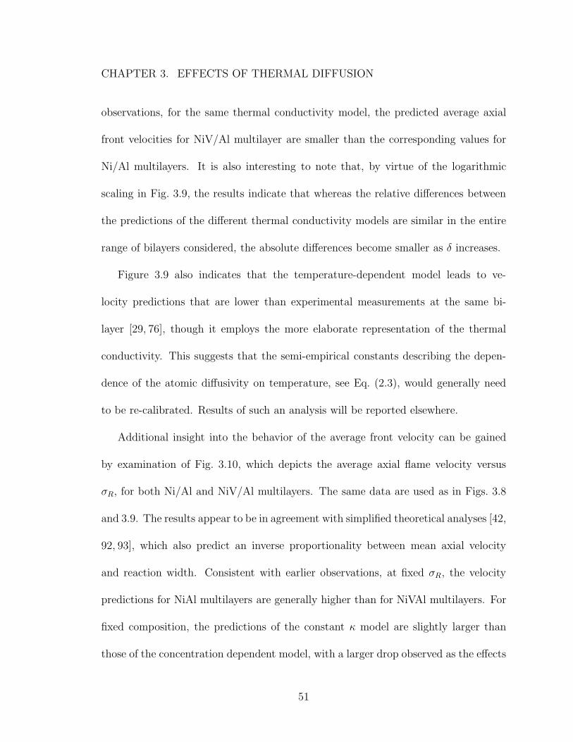
CHAPTER 3. EFFECTS OF THERMAL DIFFUSION
observations, for the same thermal conductivity model, the predicted average axial
front velocities for NiV/Al multilayer are smaller than the corresponding values for
Ni/Al multilayers. It is also interesting to note that, by virtue of the logarithmic
scaling in Fig. 3.9, the results indicate that whereas the relative differences between
the predictions of the different thermal conductivity models are similar in the entire
range of bilayers considered, the absolute differences become smaller as δ increases.
Figure 3.9 also indicates that the temperature-dependent model leads to ve-
locity predictions that are lower than experimental measurements at the same bi-
layer [29, 76], though it employs the more elaborate representation of the thermal
conductivity. This suggests that the semi-empirical constants describing the depen-
dence of the atomic diffusivity on temperature, see Eq. (2.3), would generally need
to be re-calibrated. Results of such an analysis will be reported elsewhere.
Additional insight into the behavior of the average front velocity can be gained
by examination of Fig. 3.10, which depicts the average axial flame velocity versus
σR, for both Ni/Al and NiV/Al multilayers. The same data are used as in Figs. 3.8
and 3.9. The results appear to be in agreement with simplified theoretical analyses [42,
92, 93], which also predict an inverse proportionality between mean axial velocity
and reaction width. Consistent with earlier observations, at fixed σR, the velocity
predictions for NiAl multilayers are generally higher than for NiVAl multilayers. For
fixed composition, the predictions of the constant κ model are slightly larger than
those of the concentration dependent model, with a larger drop observed as the effects
51

CHAPTER 3. EFFECTS OF THERMAL DIFFUSION
12 24 48 72 120 3000.2
0.3
0.4
0.6
0.9
1.3
2.0
3
4.0
5.5
7.0
! (nm)
Va
vg (
m/s
)
"!Constant (Ni/Al)
"!Concentration (Ni/Al)
"!Concentration+Temperature (Ni/Al)
"!Constant (NiV/Al)
"!Concentration (NiV/Al)
"!Concentration+Temperature (NiV/Al)
Figure 3.9: Average, 1D, axial flame velocity versus δ. Curves are generated for Ni/Al(solid) and NiV/Al (dashed) multilayers using the constant, concentration-dependent,and concentration and temperature dependent κ models, as indicated. In all cases,w = 0.8 nm.
52
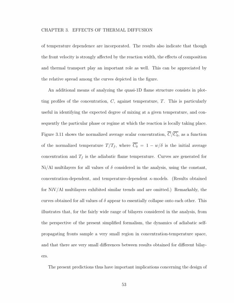
CHAPTER 3. EFFECTS OF THERMAL DIFFUSION
of temperature dependence are incorporated. The results also indicate that though
the front velocity is strongly affected by the reaction width, the effects of composition
and thermal transport play an important role as well. This can be appreciated by
the relative spread among the curves depicted in the figure.
An additional means of analyzing the quasi-1D flame structure consists in plot-
ting profiles of the concentration, C, against temperature, T . This is particularly
useful in identifying the expected degree of mixing at a given temperature, and con-
sequently the particular phase or regime at which the reaction is locally taking place.
Figure 3.11 shows the normalized average scalar concentration, C/C0, as a function
of the normalized temperature T/Tf , where C0 = 1 − w/δ is the initial average
concentration and Tf is the adiabatic flame temperature. Curves are generated for
Ni/Al multilayers for all values of δ considered in the analysis, using the constant,
concentration-dependent, and temperature-dependent κ-models. (Results obtained
for NiV/Al multilayers exhibited similar trends and are omitted.) Remarkably, the
curves obtained for all values of δ appear to essentially collapse onto each other. This
illustrates that, for the fairly wide range of bilayers considered in the analysis, from
the perspective of the present simplified formalism, the dynamics of adiabatic self-
propagating fronts sample a very small region in concentration-temperature space,
and that there are very small differences between results obtained for different bilay-
ers.
The present predictions thus have important implications concerning the design of
53

CHAPTER 3. EFFECTS OF THERMAL DIFFUSION
0.9 1.3 2 3 5 7 10 15 20 30 400.2
0.3
0.4
0.6
0.9
1.3
2
3
4
5.5
7
!R
(µm)
Va
vg (
m/s
)
"!Constant (Ni/Al)
"!Cocentration (Ni/Al)
"!Concentration+Temperature (Ni/Al)
"!Constant (NiV/Al)
"!Cocentration (NiV/Al)
"!Concentration+Temperature (NiV/Al)
Figure 3.10: Average, 1D, axial flame velocity versus σR. Curves are generated forNi/Al (solid) and NiV/Al (dashed) multilayers, using the constant, concentration-dependent, and concentration and temperature dependent κ models, as indicated.The same data points as in Figs. (3.8) and (3.9) are used.
54
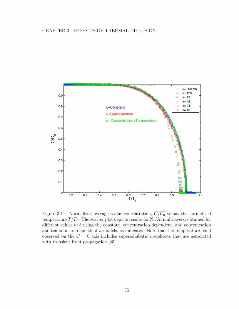
CHAPTER 3. EFFECTS OF THERMAL DIFFUSION
0.2 0.3 0.4 0.5 0.6 0.7 0.8 0.9 1 1.10
0.1
0.2
0.3
0.4
0.5
0.6
0.7
0.8
0.9
1
T/Tf
C/C
0
!= 300 nm
!= 120
!= 72
!= 48
!= 24
!= 12"!Constant
"!Concentration
"!Concentration+Temperature
Figure 3.11: Normalized average scalar concentration, C/C0 versus the normalizedtemperature T/Tf . The scatter plot depicts results for Ni/Al multilayers, obtained fordifferent values of δ using the constant, concentration-dependent, and concentrationand temperature-dependent κ models, as indicated. Note that the temperature bandobserved on the C = 0 axis includes superadiabatic overshoots that are associatedwith transient front propagation [45].
55

CHAPTER 3. EFFECTS OF THERMAL DIFFUSION
physical or computational experiments aiming at constructing simplified or reduced
models of mixing and heat release rates. Ideally, such models would provide predic-
tions for all possible values of concentration and temperature, or at least in a suitably
wide subset of the normalized concentration / normalized temperature unit square.
In this regards, the present predictions indicate that experiments on self-propagating
adiabatic fronts are not likely to sufficiently sample the resulting phase space, and
that repeated experiments with different bilayers may not necessarily shed additional
light on global mixing rates. Consequently, one should carefully consider scenarios
in which heat losses may play an important role, and/or involving different reaction
regimes. Formation reactions under spatially homogeneous conditions [31, 53, 105]
appear to be well suited for this purpose.
3.3.3 Normally-Propagating Fronts
In this section, we briefly examine the dynamics of normally propagating fronts.
Two-dimensional calculations are used for this purpose, based on small aspect ratio
domains in which the larger dimension is normal to the axis of the planes of the
bilayers. We restrict our attention to Ni/Al multilayers, and to bilayers in the range
24 nm≤ δ ≤120 nm. For this setup and front propagation regime, it is anticipated
that the effects of the directional dependence of the thermal conductivity would be
emphasized. Consequently, we will compare results from all four thermal conduc-
tivity models: the constant, concentration dependent, concentration and direction
56

CHAPTER 3. EFFECTS OF THERMAL DIFFUSION
dependent, and concentration, direction and temperature dependent κ-models. (In
the following, the latter is simply referred to as temperature-dependent model.) In
addition, we will compare the resulting predictions to earlier results obtained for ax-
ially propagating fronts. Figures 3.12 and 3.13 respectively show the reaction width
and the average front velocity as a function of δ. Plotted are curves obtained for each
of the four different κ models mentioned above.
We first note that for the constant κ model and the concentration-dependent κ
model, the thermal conductivity is isotropic. Consequently, in the context of the
present reduced reaction formalism, the simplified formulation cannot distinguish be-
tween normal and axial front propagation, and the predictions for the two propagation
modes must thus be identical. This is in fact verified in the computations. As a re-
sult, the curves for the constant and the concentration-dependent κ models are not
labeled, since they pertain to both axial and normal front propagation. This is not
necessarily the case for the direction and temperature-dependent thermal conductiv-
ity models, in which the effect of material layering is specifically accounted for. In
this situation, axial and normal fronts may have different structures. As shown in
Figs. 3.12 and 3.13, the differences between axial and normal propagation velocities
are most pronounced for the direction-dependent model.
Examination of the results further indicates that the reaction width predictions
for the constant and concentration-dependent κ models are very close. On the other
hand, the average front velocity for the constant κ model is systematically higher
57
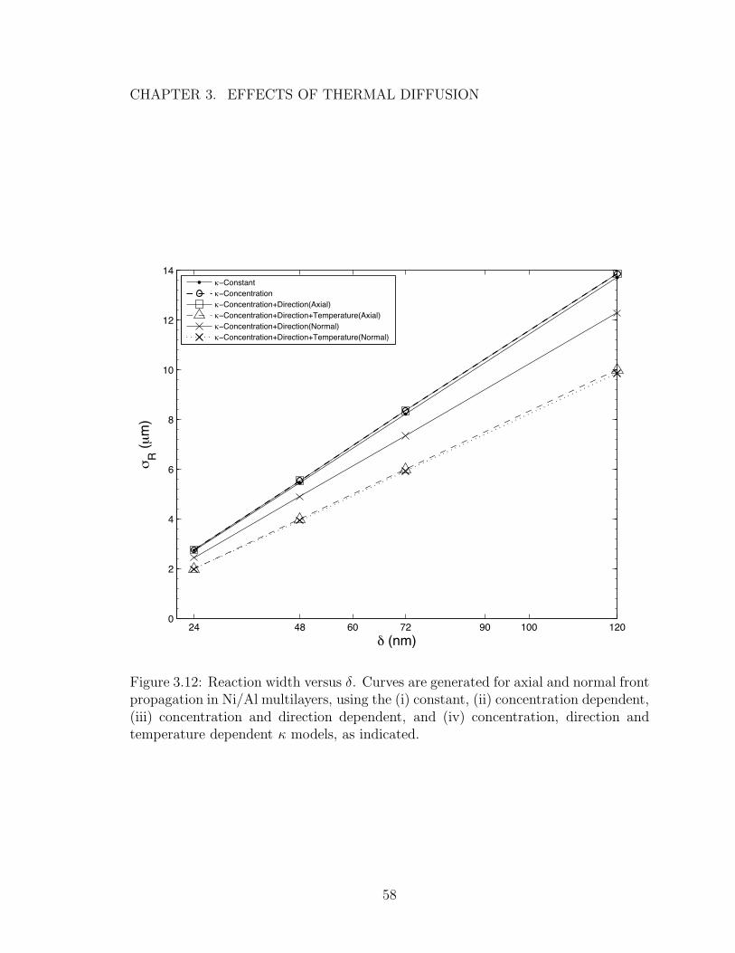
CHAPTER 3. EFFECTS OF THERMAL DIFFUSION
24 48 60 72 90 100 1200
2
4
6
8
10
12
14
! (nm)
"R
(µ
m)
#!Constant
#!Concentration
#!Concentration+Direction(Axial)
#!Concentration+Direction+Temperature(Axial)
#!Concentration+Direction(Normal)
#!Concentration+Direction+Temperature(Normal)
Figure 3.12: Reaction width versus δ. Curves are generated for axial and normal frontpropagation in Ni/Al multilayers, using the (i) constant, (ii) concentration dependent,(iii) concentration and direction dependent, and (iv) concentration, direction andtemperature dependent κ models, as indicated.
58
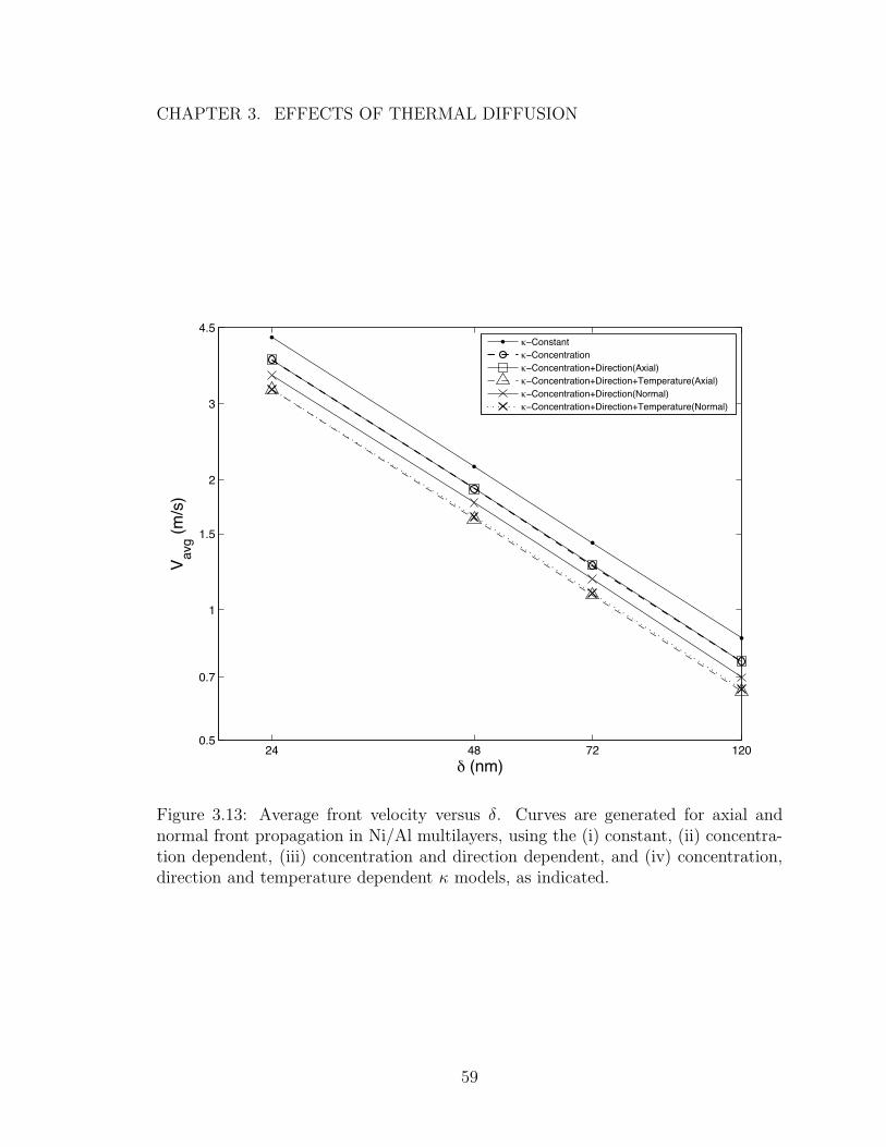
CHAPTER 3. EFFECTS OF THERMAL DIFFUSION
24 48 72 1200.5
0.7
1
1.5
2
3
4.5
! (nm)
Vavg (
m/s
)
"!Constant
"!Concentration
"!Concentration+Direction(Axial)
"!Concentration+Direction+Temperature(Axial)
"!Concentration+Direction(Normal)
"!Concentration+Direction+Temperature(Normal)
Figure 3.13: Average front velocity versus δ. Curves are generated for axial andnormal front propagation in Ni/Al multilayers, using the (i) constant, (ii) concentra-tion dependent, (iii) concentration and direction dependent, and (iv) concentration,direction and temperature dependent κ models, as indicated.
59
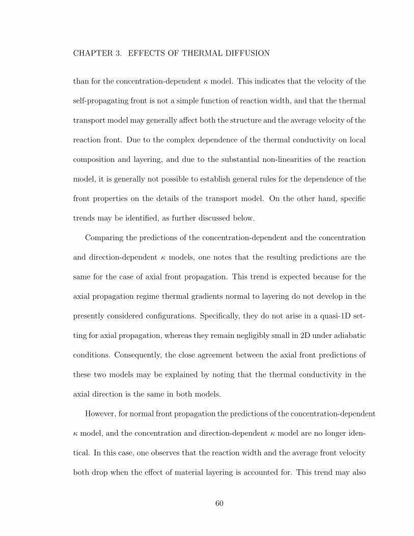
CHAPTER 3. EFFECTS OF THERMAL DIFFUSION
than for the concentration-dependent κ model. This indicates that the velocity of the
self-propagating front is not a simple function of reaction width, and that the thermal
transport model may generally affect both the structure and the average velocity of the
reaction front. Due to the complex dependence of the thermal conductivity on local
composition and layering, and due to the substantial non-linearities of the reaction
model, it is generally not possible to establish general rules for the dependence of the
front properties on the details of the transport model. On the other hand, specific
trends may be identified, as further discussed below.
Comparing the predictions of the concentration-dependent and the concentration
and direction-dependent κ models, one notes that the resulting predictions are the
same for the case of axial front propagation. This trend is expected because for the
axial propagation regime thermal gradients normal to layering do not develop in the
presently considered configurations. Specifically, they do not arise in a quasi-1D set-
ting for axial propagation, whereas they remain negligibly small in 2D under adiabatic
conditions. Consequently, the close agreement between the axial front predictions of
these two models may be explained by noting that the thermal conductivity in the
axial direction is the same in both models.
However, for normal front propagation the predictions of the concentration-dependent
κ model, and the concentration and direction-dependent κ model are no longer iden-
tical. In this case, one observes that the reaction width and the average front velocity
both drop when the effect of material layering is accounted for. This trend may also
60

CHAPTER 3. EFFECTS OF THERMAL DIFFUSION
be anticipated, since overall thermal transport normal to the layers would be more
effectively limited by the layers having highest thermal resistance.
Figures 3.12 and 3.13 also indicate that accounting for variations of the thermal
conductivities with temperature leads to appreciable drop in both the reaction width
and average front velocity. Furthermore, with the temperature-dependent κ model
there is close agreement between the predicted reaction velocities for normal and axial
front propagation. A similar trend is observed for the reaction widths. Thus, for the
presently considered system and setup, the effects of layering appear to be dominated
by the effect of thermal conductivity variation with temperature.
3.3.4 3D computations
This section briefly discusses preliminary 3D computations that implement the
presently developed generalized thermal conductivity models. We consider reactive
Ni/Al multilayers with different bilayer thicknesses, namely δ = 75 nm and δ = 6 nm.
Ignition was simulated using a localized surface heat flux that is imposed over a small
time interval [76]. Adiabatic conditions are assumed at all other times and locations.
Figure 3.14 shows instantaneous distributions of the temperature at the surface
of Ni/Al multilayer having δ = 6 nm. The computations were performed using the
temperature-dependent κ model. As can be seen in the different panels, the tempera-
ture distribution exhibits the presence of fingers that extend along the reaction front.
Observations of resolved animations (not shown) of the time-dependent temperature
61

CHAPTER 3. EFFECTS OF THERMAL DIFFUSION
field indicate that these fingers propagate in a transverse direction with respect to
the overall progress of the reaction front.
Figure 3.15 shows snapshots of the heat release rate at the surface of Ni/Al mul-
tilayer having δ = 75 nm. The computations were performed using the direction
dependent κ-model. For t ≤ 462 µs, the reaction front appears to propagate in a
uniform, steady fashion, essentially in a cylindrical fashion away from the origin.
However at later times, the two ends of the front at the domain boundaries speed
up and overtake the tip of the front, eventually creating a cusp (t = 687 µ s). The
cusp is eventually consumed, as the ends of the front touching the boundary appear
to weaken.
It is interesting to note that the transient motions observed for Ni/Al multilayers
with thin and thick bilayers bear resemblance to the recent experimental visualizations
of McDonald et al. [85,104]. In particular, the latter have revealed the occurrence of
spin-like reaction for thin bilayers, and of cellular structures for thick bilayers. The
transient structures observed in the present 3D computations appear consistent with
these observations. Unfortunately, direct comparison with measurements is not yet
possible, due to various simplifications invoked in the present computations, particu-
larly the neglect of heat losses.
On the other hand, it is interesting to note that when a constant thermal con-
ductivity model is used, the transient structures illustrated in Figs. 3.14 and 3.15 are
no longer observed. Specifically, with a constant κ model the flame front appeared
62
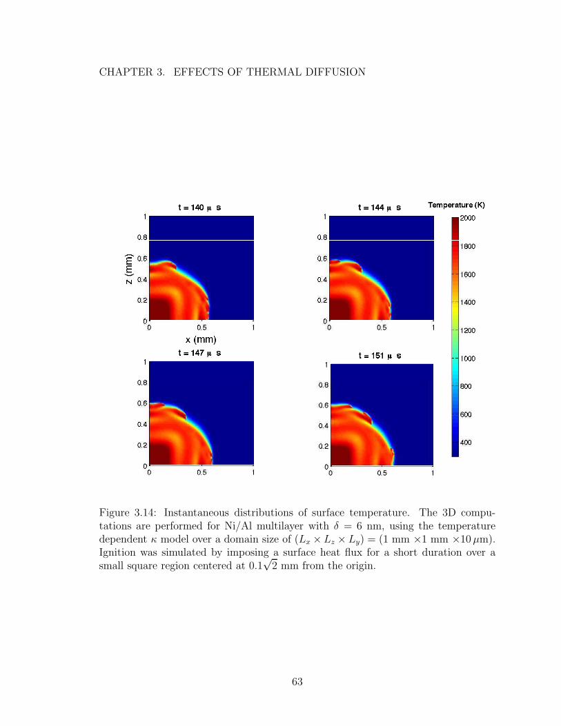
CHAPTER 3. EFFECTS OF THERMAL DIFFUSION
Figure 3.14: Instantaneous distributions of surface temperature. The 3D compu-tations are performed for Ni/Al multilayer with δ = 6 nm, using the temperaturedependent κ model over a domain size of (Lx ×Lz × Ly) = (1 mm ×1 mm ×10µm).Ignition was simulated by imposing a surface heat flux for a short duration over asmall square region centered at 0.1
√2 mm from the origin.
63
CHAPTER 3. EFFECTS OF THERMAL DIFFUSION
Figure 3.15: Instantaneous surface heat release rate profiles. The 3D computationsare performed for Ni/Al multilayer with δ = 75 nm, using the direction dependent κmodel over a domain size of (Lx × Lz × Ly) = (1 mm ×1 mm ×2µm). Ignition wassimulated by imposing a surface heat flux for a short duration over a small squareregion centered at 0.1
√2 mm from the origin.
64
CHAPTER 3. EFFECTS OF THERMAL DIFFUSION
to propagate in a uniform and steady fashion. Thus, the present results suggest
that manifestation of transient features in self-propagating front are modulated by
thermo-diffusive phenomena. Further investigations are evidently needed in order
to determine the origin of these transient features, and to characterize how their
properties depend on mixing, thermal transport, and heat losses.
65

Chapter 4
Inference of Atomic Diffusivity
4.1 Motivation
As mentioned in chapter 2, continuum approaches to modeling reaction propaga-
tion in multilayers generally rely on a simplified, phenomenological description of the
intermixing process, namely using a scalar composition field, and for the dependence
of the heat released on composition. The evolution of the composition (or conserved
scalar) is typically described in terms of a Fickian (or quasi-Fickian) process, governed
by a temperature-dependent diffusivity. The latter is assumed to follow an Arrhe-
nius law, and the pre-exponent and activation energy parameters that appear in the
corresponding expression, are usually calibrated as best fits based on experimental
measurements of the velocity of self-propagating fronts [8, 42]. With this approach,
computational models have proven to be effective at capturing the dependence of the
66
CHAPTER 4. INFERENCE OF ATOMIC DIFFUSIVITY
front velocity on composition and microstructural parameters.
However, recent experiments on low-temperature ignition and the subsequent evo-
lution of homogeneous reactions in multilayered materials have revealed that the
prevailing rates of intermixing are not consistent with those predicted by the global
Arrhenius fit of the atomic diffusivity. These investigations include the measurements
of Fritz [19], who examined the ignition of multilayer foils using electric currents and
hot plates, as well as nanocalorimetry experiments [106, 107] that have focused on
characterizing the evolution of an essentially homogeneous reaction within a single
bilayer. Consequently, it appears that the calibration of the atomic diffusivity based
on velocity observations would not lead to a diffusivity law that is valid throughout
the temperature range characterizing the reaction.
This chapter is motivated by a desire to address the above limitation. Specifically,
the questions we aim to address are: Would it be possible to combine the information
gained from low-temperature ignition experiments and from nanocalorimetry mea-
surements in order to refine the phenomenological description of intermixing rates
in continuum models? Provided this is possible, would models using the resulting
diffusivity law be able to simultaneously capture the evolution of homogeneous reac-
tions at low and intermediate temperatures, as well as the velocity of self-propagating
fronts?
Our approach towards these objectives is based on combining all sources of avail-
able information. We focus our attention on the extended reduced model formalism
67

CHAPTER 4. INFERENCE OF ATOMIC DIFFUSIVITY
discussed in chapter 3. To guide the model development, molecular dynamics com-
putations are performed in order to gain insight into the dependence of diffusivity on
temperature. Our approach for the microscale investigation is based on generalizing
the mixing measure formalism introduced by Rizzi et al. [91] for isothermal systems
to adiabatic conditions. Guided by the results of the MD analysis, we then carry
out the construction and implementation of a new composite diffusivity law based on
information gained from macroscale experimental measurements.
4.2 Atomistic Simulations
Following [91], MD simulations have been performed using LAMMPS [108]. Unless
otherwise noted, a single Ni/Al bilayer with a total thickness λ ≈ 8 nm, and δ ≈
2.34 nm is simulated by distributing Ni and Al atoms in a rectangular domain of size
≈ 53 A× 81 A × 53 A in the x, y, and z directions, respectively. Periodic boundary
conditions are imposed in all three directions in order to simulate intermixing in an
infinitely long (in the x and z directions) bilayer that periodically repeats along the
y axis. The atoms are initialized in an FCC lattice structure with the Al atoms
occupying the region 0 ≤ y ≤ 46.9 A and a lattice spacing of ≈ 4.07 A, and with the
Ni atoms occupying the region 48.8 ≤ y ≤ 78.8 A and a lattice spacing of ≈ 3.53 A.
The total number of atoms used in this arrangement is 16212, of which 8112 atoms
are Al, thus leading to a Ni/Al atomic ratio that is close to 1:1. A snapshot of the
68
CHAPTER 4. INFERENCE OF ATOMIC DIFFUSIVITY
initial system configuration is shown in Figure 4.1.
The atomic interaction potential used in the MD computations is based on the
embedded atom method (EAM) [109,110], where we specifically implement the Ni/Al
EAM/alloy potential developed by Mishin [111] and compiled by Becker et al. [112]
into a tabulated format that can readily input into LAMMPS.
The atoms are assigned initial velocities using a random Gaussian distribution
corresponding to a temperature T = 300 K, and the equations of motion are inte-
grated thereafter in three main stages: an equilibration stage, a heating stage, and
an adiabatic stage. A time step ∆t = 0.005 ps is used throughout the computations.
The first stage allows the whole system to relax to equilibrium at the desired ini-
tial conditions, and is run for a sufficiently long time using an isobaric-isothermal
NPT ensemble with pressure and temperature set to P = 0 bar and T = 300 K,
respectively. This is followed by a heating stage, also using an NPT ensemble, during
which the entire system is homogeneously heated from T = 300 K to an average
temperature T = 700 K at a rate of 0.8 K/psec. The heating stage brings the system
to a temperature that is sufficiently high for mixing to initiate within a reasonable
time-scale during the final adiabatic stage, but at the same time, still sufficiently low
so that almost no mixing occurs during the heating process. The final stage involves
integrating the system under constant pressure, constant enthalpy conditions (NPH
ensemble) with the pressure set again to P = 0 bar. During this stage, mixing of Ni
and Al atoms occurs, which is accompanied by an increase in the global average tem-
69

CHAPTER 4. INFERENCE OF ATOMIC DIFFUSIVITY
Figure 4.1: Snapshot of the initial configuration of Ni (white) and Al (green) atomsin the MD system at time t = 0. The arrangement corresponds to a Ni/Al bilayer oftotal thickness λ = 8 nm and δ = 2.34 nm.
70

CHAPTER 4. INFERENCE OF ATOMIC DIFFUSIVITY
perature of the closed system due to the exothermic nature of the mixing process. The
integration is carried out until a state of complete mixing is achieved which, for the
given system size, required around 4.4 million NPH integration steps. In both NPT
(NPH) ensembles, the temperature (enthalpy) and pressure of the system are main-
tained close to the desired mean values using the Nose-Hoover formalism [113–115]
with a relaxation timescale of 2 ps.
4.2.1 Coarse graining
The output of the adiabatic MD simulation runs allows us to monitor the evolution
of the global average kinetic temperature of the system, along with the evolution of
the instantaneous position of each atom. However, the parameter that we are seeking
to extract is D(T ), which is an effective diffusivity parameter that does not depend on
space nor on the particle identity. Consequently, this requires us to perform a coarse-
graining step in order to estimate D(T ). For this purpose, we adopt the mixing
measure formalism developed by Rizzi et al. [91], which relies on first calculating
the instantaneous cumulative distribution function (CDF) of each atom type, defined
according to:
Fi(y0, t) ≡ ni(y ≤ y0; t)
Ni
, i = Ni, Al, (4.1)
where ni is the number of atoms of type i whose position in the y-direction at time
t lies in the range 0 ≤ y ≤ y0, with 0 ≤ y0 ≤ λ. Ni is the total number of atoms of
type i, which is a constant for our NPT and NPH ensemble simulations. The Ni and
71

CHAPTER 4. INFERENCE OF ATOMIC DIFFUSIVITY
Al CDFs are then used to define an instantaneous mixing measure, M , such that:
M(t) ≡ 1
2
∫ λ
0
∣
∣
∣
∣
∂FNi
∂y− 1
λ
∣
∣
∣
∣
+
∣
∣
∣
∣
∂FAl
∂y− 1
λ
∣
∣
∣
∣
dy (4.2)
where ∂FNi/∂y and ∂FAl/∂y are the instantaneous probability distributions of the
Ni and Al atoms respectively, and 1/λ is the probability distribution corresponding
to a homogeneous, ideally-mixed system. In our MD simulations, the system starts
out in an unmixed state corresponding to compositionally pure layers, and eventually
relaxes towards equilibrium given by a fully-mixed state. Thus, according to the
definition in (4.2), M(t) evolves from an initial value of M(t = 0) = 1 to a value of
M = 0 when complete mixing is achieved.
The above coarse-grained formalism allows us to describe the evolution of the
microscopic dynamics using a measure, M , that is equivalent to the continuum average
scalar concentration, C. Consequently, through a direct mapping of M(t) to the
continuum concentration evolution equation given by equation (2.1), one can infer
the dependence of the diffusivity, D, on temperature. Details of the mapping and
inference procedures are outlined below.
4.2.2 Extracting D(T )
It has been shown in [31] that by (i) assuming that atomic diffusion is dominant
across the layers (in the y-direction), and (ii) exploiting the separation of length and
72

CHAPTER 4. INFERENCE OF ATOMIC DIFFUSIVITY
time scales over which atomic and thermal diffusion occur, Eq. (2.1) simplifies to:
∂C
∂t= D(T )
∂2C
∂y2(4.3)
and can be recast into approximate canonical form:
∂C
∂τ=
∂2C
∂ξ2(4.4)
where ξ ≡ y/δ is a normalized spatial variable, and τ is the normalized stretched
time variable defined in Eq. (2.10). For an initially unmixed system, the solution of
the canonical equation (4.4) can be expressed in terms of a Fourier-sine series of the
form [31]:
C(ξ, τ) =n=∞∑
n=1
2
anexp
(
−a2nτ)
sin (anξ) (4.5)
where
an =(2n− 1)π
2
Using equation (4.5), we can obtain the first moment of the concentration, C(τ),
according to:
C(τ) =
∫ 1
0
C(ξ, τ) dξ =1
δ
∫ δ
0
C(y, τ) dy
=
n=∞∑
n=1
2
a2nexp
(
−a2nτ)
(4.6)
As mentioned previously, our aim is to first map M(t) from MD to the concentration
evolution equation, which has now been simplified into equation (4.3). Consequently,
we need to transform the evolution equation for C into an evolution equation for M .
73

CHAPTER 4. INFERENCE OF ATOMIC DIFFUSIVITY
In order to achieve this, knowing that M is a measure that is equivalent to C, we
average equation (4.3) over δ in the y-direction to obtain:
1
δ
∫ δ
0
∂C
∂tdy =
1
δ
∫ δ
0
D(T )∂2C
∂y2dy
Since C and ∂C/∂t are both continuous and bounded, we can exchange the order of
integration and the time-derivative, which yields:
∂
∂t
(
1
δ
∫ δ
0
C dy
)
=1
δ
∫ δ
0
D(T )∂2C
∂y2dy
Finally, evaluating the right hand side and noting that M(t) ≡ C(t), we get:
∂C
∂t=
∂M
∂t= − D(T )
δ
∂C
∂y
∣
∣
∣
∣
y=0
(4.7)
Differentiating equation (4.5) with respect to ξ we have:
∂C
∂y
∣
∣
∣
∣
y=0
=1
δ
∂C
∂ξ
∣
∣
∣
∣
ξ=0
=1
δ
n=∞∑
n=1
2 exp(
−a2nτ)
(4.8)
In order to complete our analysis, we still need to compute τ . To this end, we
note that since M(τ) is to be identified with C(τ), we can use Eq. (4.6), along
with our knowledge of M(t) from MD, in order to appropriately interpolate for the
corresponding value of τ . Equation (4.7) can then be directly used for our main
74
CHAPTER 4. INFERENCE OF ATOMIC DIFFUSIVITY
objective of extracting D(T ), namely according to:
D(T ) = − δ
∂M
∂t∂C
∂y
∣
∣
∣
∣
y=0
= − δ2
∂M
∂tn=∞∑
n=1
2 exp(
−a2nτ)
(4.9)
Note that one cannot compute τ from the definition given by Eq. (2.10), since the
diffusivity D depends on temperature which, in our NPH MD simulations, is a time
dependent variable. Moreover, D(T ) is an unknown that we are trying to estimate.
4.3 Results
In this section, we start by applying the MD computations described in section 4.2
to analyze the behavior of homogeneous reactions under adiabatic conditions, and im-
plement the formalism outlined in sections 4.2.1 and 4.2.2 in order to infer the the
atomic diffusivity, D(T ). As further discussed below, when incorporated into the re-
duced model, the MD predictions of D(T ) lead to estimates of self-propagating front
velocities that exhibit large discrepancies with experimental observations and previ-
ous computational estimates. Consequently, the qualitative trends resulting from the
MD analysis are used in conjunction with macroscale measurements in order to con-
struct a suitable composite atomic diffusivity correlation. These include observations
obtained from homogeneous current ignition experiments [19], nanocalorimetry ex-
75

CHAPTER 4. INFERENCE OF ATOMIC DIFFUSIVITY
periments [106, 107], and self-propagating reaction front velocity measurements [29],
which respectively inform us on the behavior of intermixing rates at low, intermediate,
and high temperatures.
4.3.1 MD analysis
Integrating the equations of motion in an NPT and NPH ensemble allows us to
predict the time evolution of the instantaneous positions of all the atoms in the system,
along with that of the average thermodynamic properties such as temperature. Using
this information in conjunction with Eqs. (4.1) and (4.2), we can obtain the time
evolution of the mixing measure M(t). To investigate the potential dependence of
the inferred diffusivity on the bilayer thickness, and consequently the suitability of
the quasi-Fickian model to describe the evolution of the mixing measure, we consider
two MD systems with δ = 2.34 nm and δ = 4.78 nm.
Figure 4.2 shows instantaneous CDF profiles obtained for δ = 2.34 nm. Plotted
are curves corresponding to the initial time, t = 0, and to a time, t = 2.2× 10⁴ psec,
during which the system is approaching the equilibrium, fully-mixed state. Ideal
mixing, corresponding to a uniform distribution of the Al and Ni atoms, is depicted
using a dashed line. Fig. 4.3 shows the evolution of the mixing measure, M , during the
equilibration, heating, and adiabatic stages. The evolution of the average temperature
of the system is shown in Fig. 4.4. Note that by the end of the NPT heating stage
(t = 0.3×10⁴ psec), the mixing measure has dropped by less than 3% (Fig. 4.3). Thus,
76
CHAPTER 4. INFERENCE OF ATOMIC DIFFUSIVITY
most of the mixing occurs during the NPH stage, which enables us to characterize
interdiffusion and heat generation rates under adiabatic conditions, in essentially the
entire range of M .
77

CHAPTER 4. INFERENCE OF ATOMIC DIFFUSIVITY
0 0.2 0.4 0.6 0.8 10
0.2
0.4
0.6
0.8
1
y/λ
Fi(y
,t)
0 0.2 0.4 0.6 0.8 10
0.2
0.4
0.6
0.8
1
y/λ
Fi(y
,t)Al
Ni
Ni
Al
(a) t = 0 psec (b) t = 2.2× 10⁴ psec
Figure 4.2: Cumulative distribution functions (CDF) of Nickel (red) and Aluminum(blue), computed at (a) t = 0, and (b) t = 2.2 × 10⁴ psec. The dashed line y = xcorresponds to the asymptotic limit of a completely mixed system.
78

CHAPTER 4. INFERENCE OF ATOMIC DIFFUSIVITY
0 0.5 1 1.5 2 2.5
x 104
0
0.1
0.2
0.3
0.4
0.5
0.6
0.7
0.8
0.9
1
Time (psec)
M
Equilibration
Heating
Adiabatic
2.15 2.2 2.25 2.3
x 104
0
0.1
0.2
0.3
0.4
0.5
Figure 4.3: Mixing measure versus time for an MD system with δ = 2.34 nm. Thecurves depicts the evolution of M(t) during the initial equilibration stage, the rapidheating stage to T = 700 K, and the adiabatic stage. Inset provides an enlarged viewof the late stages of the computations, during which the Ni structure collapses.
79

CHAPTER 4. INFERENCE OF ATOMIC DIFFUSIVITY
0 0.5 1 1.5 2 2.5 3 3.5 4 4.5
x 104
200
400
600
800
1000
1200
1400
1600
1800
Time (psec)
Te
mp
era
ture
(K
)
2.15 2.2 2.25 2.3
x 104
1400
1500
1600
1700
1800
Adiabatic starts
Heating starts
Figure 4.4: Average temperature versus time for an MD system with δ = 2.34 nm.The curves depicts the evolution of T (t) during the initial equilibration stage, therapid heating stage to T = 700 K, and the adiabatic stage. Inset provides an enlargedview of the late stages of the computations, during which the Ni structure collapses.
80
CHAPTER 4. INFERENCE OF ATOMIC DIFFUSIVITY
Based on the evolutions of temperature and mixing measure, Eq. (4.9) is used
to infer the atomic diffusivity D(T ). The results are plotted in Fig. 4.5 for both
δ = 2.34 nm, and δ = 4.78 nm. Note that the inference is restricted to the NPH stage
only. As can be seen from Fig. 4.5, the results for δ = 2.34 nm and δ = 4.78 nm
are in close agreement for most of the temperature range, with small but noticeable
differences at high temperatures. Specifically, the curve for δ = 2.34 nm exhibits
a discontinuous jump as the system approaches equilibrium, whereas the curve for
δ = 4.78 nm follows a smoother rise. Overall, however, the diffusivity predictions are
weakly dependent on the selected system size.
Note that the inferred diffusivity values exhibit a scatter in the temperature range
T ≈ 770−880K. This coincides with the region in Fig. 4.4 around which a sudden dip
in the average global temperature is observed. Visualization of the MD simulations
reveals that by this time, some of the Ni atoms have diffused into the Al region, leaving
a narrow block of structured (solid) Al that is just a few atoms thick. The sudden
decrease in temperature and the scatter in the inferredD values occur around the time
that the thin Al block loses its initial structure. We also relied on visualization of the
MD computations to examine the origin of the sudden jump in the inferred D values
for δ = 2.34 nm around T = 1570K. The simulations revealed that this coincides with
the collapse of the remaining Ni structure, after which complete mixing is reached
very rapidly. This also coincides with the switch in the curvature of the curve for
the mixing measure (inset in Fig. 4.3) and the sudden rise in temperature (inset in
81
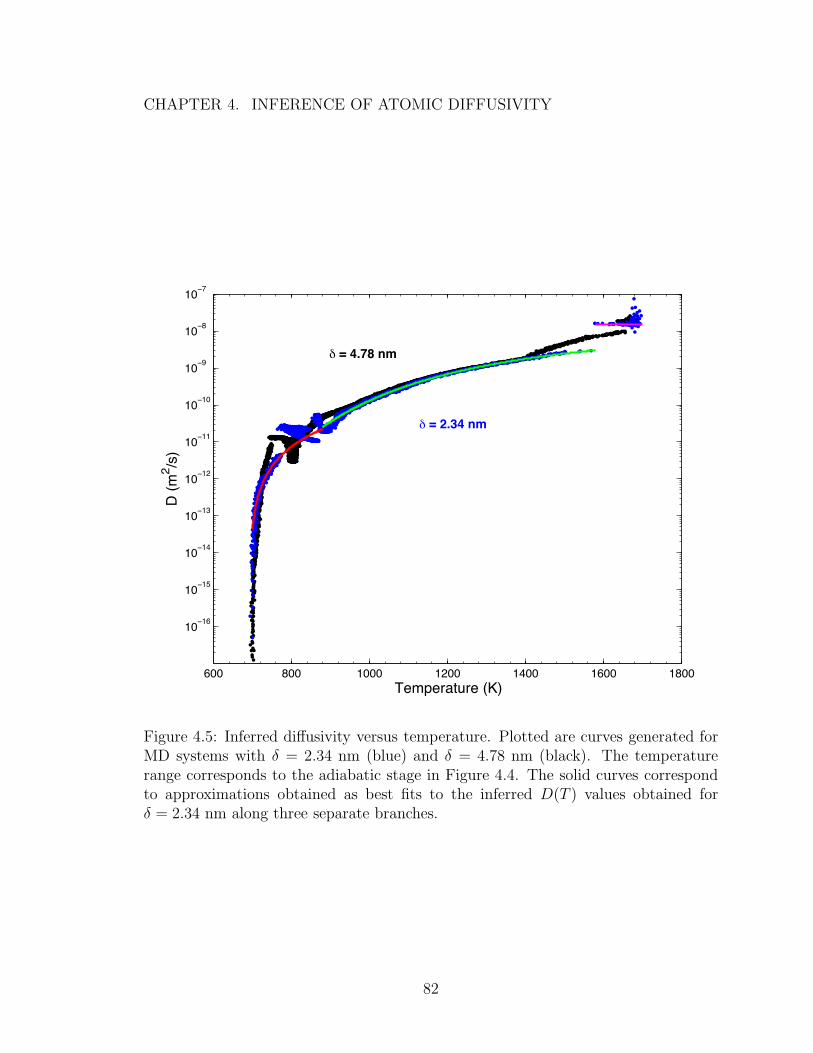
CHAPTER 4. INFERENCE OF ATOMIC DIFFUSIVITY
600 800 1000 1200 1400 1600 1800
10−16
10−15
10−14
10−13
10−12
10−11
10−10
10−9
10−8
10−7
Temperature (K)
D (
m2/s
)
δ = 4.78 nm
δ = 2.34 nm
Figure 4.5: Inferred diffusivity versus temperature. Plotted are curves generated forMD systems with δ = 2.34 nm (blue) and δ = 4.78 nm (black). The temperaturerange corresponds to the adiabatic stage in Figure 4.4. The solid curves correspondto approximations obtained as best fits to the inferred D(T ) values obtained forδ = 2.34 nm along three separate branches.
82
CHAPTER 4. INFERENCE OF ATOMIC DIFFUSIVITY
Fig. 4.4).
To verify the MD-predictions of D(T ), an approximate fit of the individual data
plotted in Fig. 4.5 was first obtained for incorporating into the continuum model.
Attention was focused on the results obtained for δ = 2.34 nm, and the MD-based
results were interpolated using three separate branches, respectively approximating
the data during the initial rapid rise, the monotonic increase after Al loses its initial
structure, and the constant cluster of data observed after the collapse of Ni. The
resulting composite fit is also depicted in Fig. 4.5. Note that in constructing the
composite fit we ignore the scatter in D(T) in the temperature range T = 770−880K.
In order to carry out our verification step, and check whether we can recover the time
evolution of the mixing measured observed in the MD simulations (Fig. 4.3) using our
smoothed D(T) approximations, we (i) insert the fits forD(T ) into Eq. (2.12), and (ii)
integrate the resulting equation using the temperature evolution obtained from the
MD simulation (Fig. 4.4). Fig. 4.6 contrasts the resulting reduced model prediction
for M(t) with the results obtained from the MD simulations. As can be seen from
the figure, the reduced model solution using the D(T ) fits successfully reproduces
the MD-computed evolution of the mixing measure, thus lending confidence in our
inference scheme and in the resulting smoothed composite fit.
In addition to inferring D(T ), we have also relied on the MD computations to
explore the dependence of the reaction heat on the mean concentration (or mixing
measure). Recall that the original formulation of the continuum model relied on a
83
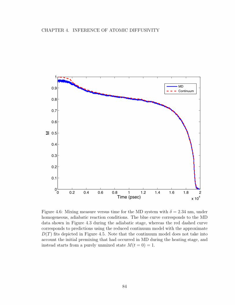
CHAPTER 4. INFERENCE OF ATOMIC DIFFUSIVITY
0 0.2 0.4 0.6 0.8 1 1.2 1.4 1.6 1.8 2
x 104
0
0.1
0.2
0.3
0.4
0.5
0.6
0.7
0.8
0.9
1
Time (psec)
M
MD
Continuum
Figure 4.6: Mixing measure versus time for the MD system with δ = 2.34 nm, underhomogeneous, adiabatic reaction conditions. The blue curve corresponds to the MDdata shown in Figure 4.3 during the adiabatic stage, whereas the red dashed curvecorresponds to predictions using the reduced continuum model with the approximateD(T ) fits depicted in Figure 4.5. Note that the continuum model does not take intoaccount the initial premixing that had occurred in MD during the heating stage, andinstead starts from a purely unmixed state M(t = 0) = 1.
84
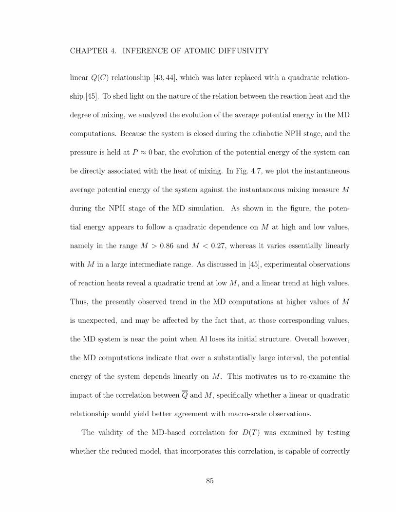
CHAPTER 4. INFERENCE OF ATOMIC DIFFUSIVITY
linear Q(C) relationship [43, 44], which was later replaced with a quadratic relation-
ship [45]. To shed light on the nature of the relation between the reaction heat and the
degree of mixing, we analyzed the evolution of the average potential energy in the MD
computations. Because the system is closed during the adiabatic NPH stage, and the
pressure is held at P ≈ 0 bar, the evolution of the potential energy of the system can
be directly associated with the heat of mixing. In Fig. 4.7, we plot the instantaneous
average potential energy of the system against the instantaneous mixing measure M
during the NPH stage of the MD simulation. As shown in the figure, the poten-
tial energy appears to follow a quadratic dependence on M at high and low values,
namely in the range M > 0.86 and M < 0.27, whereas it varies essentially linearly
with M in a large intermediate range. As discussed in [45], experimental observations
of reaction heats reveal a quadratic trend at low M , and a linear trend at high values.
Thus, the presently observed trend in the MD computations at higher values of M
is unexpected, and may be affected by the fact that, at those corresponding values,
the MD system is near the point when Al loses its initial structure. Overall however,
the MD computations indicate that over a substantially large interval, the potential
energy of the system depends linearly on M . This motivates us to re-examine the
impact of the correlation between Q and M , specifically whether a linear or quadratic
relationship would yield better agreement with macro-scale observations.
The validity of the MD-based correlation for D(T ) was examined by testing
whether the reduced model, that incorporates this correlation, is capable of correctly
85

CHAPTER 4. INFERENCE OF ATOMIC DIFFUSIVITY
0 0.1 0.2 0.3 0.4 0.5 0.6 0.7 0.8 0.9 1−6.4
−6.35
−6.3
−6.25
−6.2
−6.15x 10
4
M
PE
(eV
)
Figure 4.7: Average potential energy of the MD system with δ = 2.34 nm versus themixing measure, M , during the adiabatic phase.The M values correspond to thoseshown in Fig. 4.3 during the adiabatic stage.
86

CHAPTER 4. INFERENCE OF ATOMIC DIFFUSIVITY
capturing average velocity of self-propagating reaction fronts. Unfortunately, all at-
tempts at directly using the atomic diffusivity correlations inferred from MD resulted
in continuum predictions that failed to correctly reproduce experimental observations,
specifically leading to computed velocities (not shown) that are several folds faster
than the measurements. Such discrepancies are a clear indication that the MD-based
correlations significantly overestimate intermixing rates. This represents a substantial
drawback for the present MD computations, especially since continuum formulations
using an empirically calibrated diffusivity law [31,41,76] can successfully capture the
velocity of self-propagating fronts, as well as their dependence on the bilayer thick-
ness. An additional drawback of the MD computations is that the predicted increase
in temperature due to the reaction, ∆Tf , exhibited in Fig. 4.4 also underestimates
the values computed based on reaction heats. Note that, even when the lower ∆Tf
predicted by MD is accounted for when using the MD D(T ) correlations, the resulting
continuum predictions still tend to markedly over-estimate the average front veloci-
ties. These shortcomings constitute a substantial hurdle facing the use of the present
MD computations for the purpose of formulating or calibrating continuum models
that can reproduce experimental observations with sufficient fidelity.
In an attempt to identify a possible source for the errors mentioned above, we have
briefly examined whether the MD-inferred diffusivity values are considerably affected
by the details of the inter-atomic potentials that govern the evolution of the system.
To this end, the inference of the diffusivity law was repeated based on MD simulations
87

CHAPTER 4. INFERENCE OF ATOMIC DIFFUSIVITY
that implement the more recent version of the Ni/Al EAM/alloy inter-atomic poten-
tial [116]. This, however, led to atomic diffusivity values that are even higher than
those depicted in Fig. 4.5, and consequently to even larger discrepancies between the
associated front velocity predictions and experimental observations. While the exer-
cise demonstrates that the details of the inter-atomic potential can have substantial
impact on the predicted average properties of the system, no attempt was made in
this effort at refining the MD potentials, or at developing a more sophisticated MD
model that would, for instance, account for additional factors such as the presence of
impurities, the impact of heat losses, and the presence of an initial premix region.
Considering the shortcomings of the MD inferred atomic diffusivity values, we
have opted alternatively to exploit merely the qualitative trends provided by the MD
computations regarding the variation of D with temperature. Specifically, the MD
computations reveal that the diffusivity could increase rapidly and even exhibit dis-
continuities at certain critical temperatures. Therefore in what follows, we explore
using these trends in order to formulate a generalized diffusivity law, and to infer the
corresponding parameters by relying on experimental observations of homogeneous
current ignition, nanocalorimetry, and reaction front velocities. Moreover, as men-
tioned above, based on the largely linear dependence of Q on C suggested by MD,
we look into whether a linear or quadratic relationship is a more suitable assumption
to use with the newly generalized diffusivity law.
88

CHAPTER 4. INFERENCE OF ATOMIC DIFFUSIVITY
4.4 Macroscale Information
4.4.1 Low Temperature Regime
In this subsection, we aim to infer atomic diffusivity values at the low temperature
end. We rely on the homogeneous current ignition experiments of Fritz [19] for this
purpose. The experiments were conducted in air using sputter-deposited (1:1) NiV/Al
multilayers with δ ≈ 56 nm and total thickness of approximately 19µm. Ignition was
triggered by driving, along the foil length, a constant current pulse with a current
density of 111 kA/m2. The current was maintained for a 5 msec interval and then
abruptly turned off. This resulted in essentially uniform heating of the foil to a
temperature of about 543 K. Following the Joule heating stage, the foil was allowed
to react freely. The temperature on the foil surface was monitored during the entire
process using an optical pyrometer with a response time of 40 µs and a temperature
sensitivity range of T = 473−1273 K. Assuming that the atomic diffusivity exhibits an
Arrhenius dependence on temperature, the corresponding values of the pre-exponent,
D0, and activation energy Ea, have been inferred numerically based on the measured
evolution of the surface temperature.
To this end, the reduced continuum model given by Eqs. (2.12)–(2.14) was imple-
mented in order to simulate the system response under homogeneous, non-adiabatic
conditions. The latter arises because the experiments were carried out in open air,
leading us to account for convective heat losses. This was modeled using a heat trans-
89

CHAPTER 4. INFERENCE OF ATOMIC DIFFUSIVITY
fer coefficient, which was considered to be equivalent to that of a hot horizontal flat
plate facing upwards [19]. Note that on the order of the length and time scales con-
cerned, radiative heat losses are negligible in comparison with convective heat losses,
and were therefore ignored.
The finite-difference numerical scheme developed in [74] was adapted for solving
the resulting system of differential equations. The impact of the Joule heating was
modeled using an equivalent volumetric source term, which resulted in an essentially
the same rise in the foil temperature as was observed in the experiments. In our
implementation of the reduced model, we accounted for the presence of Vanadium
in the multilayers by matching the experimentally measured reaction heats [29, 100],
namely ∆Hrxn = 1200 J/g. Accordingly, the nominal temperature change due to the
reaction is estimated using ∆Tf = ∆Hrxn/cp, where cp is the foil mean specific heat
capacity. The average concentration was initialized using C(t = 0) = 1−w/δ, with a
constant premix width of w = 0.8 nm [29,76]. Finally, based on the MD observations
reported in the previous section, we used a linear dependence of the reaction heat on
the mean concentration.
In order to determine the Arrhenius diffusivity parameters, D0 and Ea, a non-
linear gradient-free multivariate direct search optimization technique based on the
simplex algorithm was implemented. The technique aims at minimizing an objective
function given by the mean-squared error between the experimental temperature ob-
servations, Texp(t), and the temperature evolution predicted by the reduced model,
90

CHAPTER 4. INFERENCE OF ATOMIC DIFFUSIVITY
Tnum(t). The optimization is carried out iteratively, where a feedback loop is estab-
lished between the optimization code, which updates D0 and Ea, and the reduced
model code, which provides the temperature evolution, Tnum(t). The iterations are
carried out until the objective function converges to a desired minimum tolerance
value. The optimization procedure was constrained over temperatures T ≤ 800 K,
due to the low time resolution of the homogeneous current ignition experiments at
higher temperatures.
Figure 4.8 shows the observed experimental temperature evolution by Fritz [19]
(solid curve), along with predictions (dashed curve) using the reduced continuum
model with the optimized pre-exponential and activation energy values, D0 = 2.08×
10−7 m2/s and Ea = 92.586 kJ/mol. The impact of using a quadratic versus a
linear assumption for the heat released by the reaction on the resulting D(T ) values
is illustrated in Fig. 4.9. Note that the curves obtained using linear and quadratic
dependence are in close agreement for temperatures smaller than about 500 K, but
that they then diverge noticeably as the temperature increases. Also plotted for
comparison in Fig. 4.9 is the D(T ) correlation obtained by Fritz [19], namely using an
Arrhenius relationship with D0 = 5.58×10⁻⁹ m2/s and Ea = 78.9 kJ/mol. Noticeable
differences from the present predictions can be observed at low and high temperatures.
To gain insight into the differences between the predictions, one should first recall
that during the period of the electric discharge, the Joule heating dominates the total
energy released; this can be appreciated by the fact that the rate of the temperature
91

CHAPTER 4. INFERENCE OF ATOMIC DIFFUSIVITY
0 0.005 0.01 0.015 0.02 0.025 0.03 0.035200
400
600
800
1000
1200
1400
1600
1800
2000
Time (sec)
Te
mp
era
ture
(K
)
Experimental
Reduced Model
0.005 0.01 0.015 0.02 0.025 0.03
550
600
650
700
750
800
Low Temperature
Regime
Figure 4.8: Temperature evolution with time for a homogeneous reaction regime ina NiV/Al multilayer with δ = 56 nm. The blue curve corresponds to experimentalobservations by Fritz [19], while the red dashed curve corresponds to predictions (trun-cated at T = 800 K) using the reduced continuum model with optimized pre-exponentand activation energy values, D0 = 2.08× 10⁻⁷m2/s and Ea = 92.586 kJ/mol. Insetprovides a zoom into the optimized region following the heating stage.
92
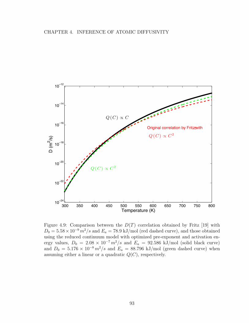
CHAPTER 4. INFERENCE OF ATOMIC DIFFUSIVITY
300 350 400 450 500 550 600 650 700 750 80010
−24
10−22
10−20
10−18
10−16
10−14
10−12
Temperature (K)
D (
m2/s
)
Q (C ) ∝ C
Q (C ) ∝ C 2
Q (C ) ∝ C 2
Original correlation by Fritz with
Figure 4.9: Comparison between the D(T ) correlation obtained by Fritz [19] withD0 = 5.58×10⁻⁹m2/s and Ea = 78.9 kJ/mol (red dashed curve), and those obtainedusing the reduced continuum model with optimized pre-exponent and activation en-ergy values, D0 = 2.08 × 10⁻⁷m2/s and Ea = 92.586 kJ/mol (solid black curve)and D0 = 5.176 × 10⁻⁸m2/s and Ea = 88.796 kJ/mol (green dashed curve) whenassuming either a linear or a quadratic Q(C), respectively.
93
CHAPTER 4. INFERENCE OF ATOMIC DIFFUSIVITY
rise drops dramatically as the current is switched off. As a result, the diffusivity esti-
mates obtained at temperatures lower than the temperature reached by the system at
the end of the electrical discharge (543 K) are effectively extrapolated values from the
range that is actually inferred by the analysis. Thus, it is only appropriate to com-
pare predictions at the higher temperatures. Focusing first on the present estimates,
one notes that with a linear dependence of Q on C, higher diffusivity estimates are
obtained than with a quadratic dependence. This is expected since, for an essentially
unmixed system, the rate of change of Q with C is smaller for a linear dependence
than it is for a quadratic dependence. Turning now our attention to the predictions
of Fritz, we first note that the analysis in [19] ignored the presence of Vanadium, and
consequently used a higher reaction heat, and used a different procedure that simply
aimed at optimizing D0 with a fixed value of the activation energy. Not surprisingly,
in the range T > 550 K, the inferred diffusivities obtained in [19] reveal lower val-
ues than the current reduced model predictions, and the nature of the discrepancy
appears to be largely due to the different reaction heats. Combined, the present expe-
riences underscore the fact that the inferred estimates may be substantially affected
by the details and fidelity of the underlying physical model.
94
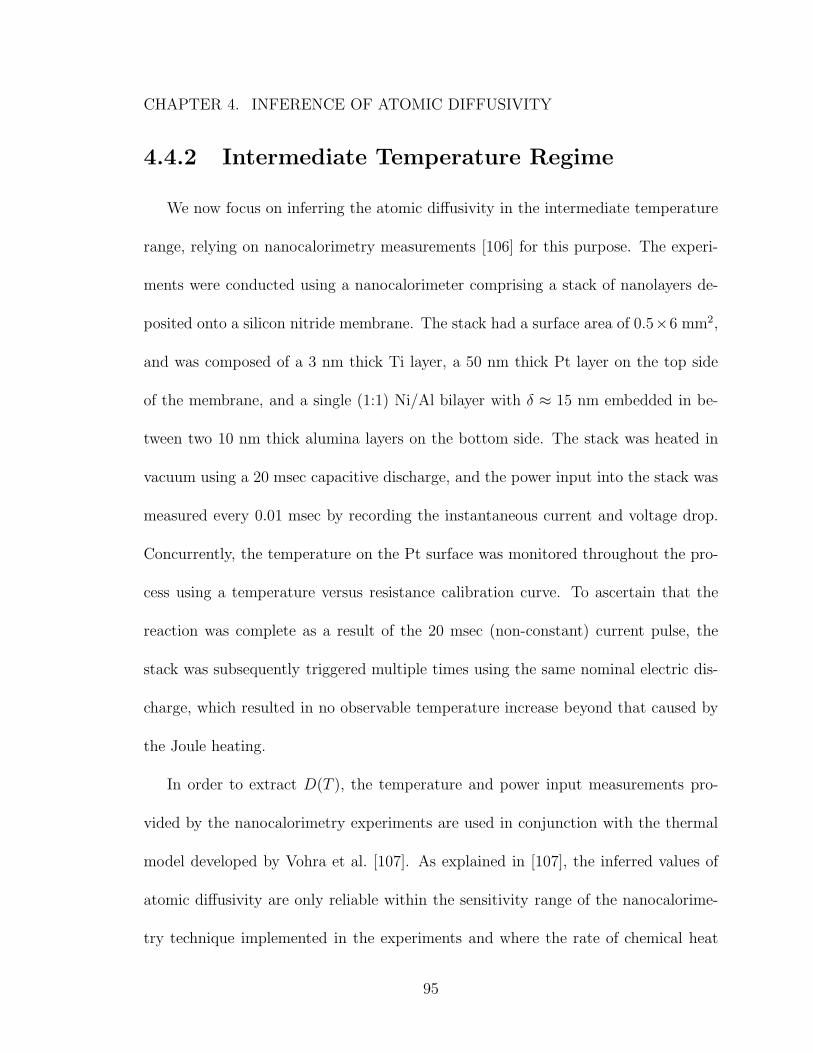
CHAPTER 4. INFERENCE OF ATOMIC DIFFUSIVITY
4.4.2 Intermediate Temperature Regime
We now focus on inferring the atomic diffusivity in the intermediate temperature
range, relying on nanocalorimetry measurements [106] for this purpose. The experi-
ments were conducted using a nanocalorimeter comprising a stack of nanolayers de-
posited onto a silicon nitride membrane. The stack had a surface area of 0.5×6 mm2,
and was composed of a 3 nm thick Ti layer, a 50 nm thick Pt layer on the top side
of the membrane, and a single (1:1) Ni/Al bilayer with δ ≈ 15 nm embedded in be-
tween two 10 nm thick alumina layers on the bottom side. The stack was heated in
vacuum using a 20 msec capacitive discharge, and the power input into the stack was
measured every 0.01 msec by recording the instantaneous current and voltage drop.
Concurrently, the temperature on the Pt surface was monitored throughout the pro-
cess using a temperature versus resistance calibration curve. To ascertain that the
reaction was complete as a result of the 20 msec (non-constant) current pulse, the
stack was subsequently triggered multiple times using the same nominal electric dis-
charge, which resulted in no observable temperature increase beyond that caused by
the Joule heating.
In order to extract D(T ), the temperature and power input measurements pro-
vided by the nanocalorimetry experiments are used in conjunction with the thermal
model developed by Vohra et al. [107]. As explained in [107], the inferred values of
atomic diffusivity are only reliable within the sensitivity range of the nanocalorime-
try technique implemented in the experiments and where the rate of chemical heat
95

CHAPTER 4. INFERENCE OF ATOMIC DIFFUSIVITY
release is an increasing function of time, namely 720 ≤ T ≤ 860 K. For the sake of
completeness, a brief outline of the thermal model is given below. Further details on
the model can be found in [107].
The thermal model as developed in [107] revolves around the assumption that the
nanocalorimeter stack (including the silicon nitride membrane) can be analyzed using
a lumped model. The model exploits the construction of the device and its operating
conditions, and consequently ignores convective and conductive heat losses. Due to
the small stack thickness, however, radiative heat losses are retained. Furthermore,
since the inferred values adopted are limited to a temperature range falling below the
melting temperature of Al, melting effects need not be accounted for. Accordingly, on
the timescale of the experiment, the temperature within the nanocalorimeter stack is
governed by the following, simplified, volume-averaged energy equation:
(ρcp)s Vs
dT
dt= V ∂Q
∂t+∆φI − σ (ǫtAt + ǫbAb)
(
T 4 − T 40
)
(4.10)
where (ρcp)s and Vs respectively denote the mean specific heat and volume of the
stack. The three source terms on the right-hand-side of Eq. (4.10) correspond to
the rate of heat released by the reaction, the Joule heating, and the radiation loss.
The Joule heating term is expressed in terms of the current (I) and voltage drop
(∆φ) across the stack; both values are obtained from the experimental measurements.
The last term term represents gray body radiative heat losses, derived under the
assumption that losses from the sides of the stack are negligible compared to those
from the top surface and bottom surfaces. Here, σ is the Stefan-Boltzmann constant,
96

CHAPTER 4. INFERENCE OF ATOMIC DIFFUSIVITY
ǫ is the emissivity, A is the surface area of the stack, the subscripts t and b refer to the
top and bottom surfaces of the stack respectively, and T0 is the ambient temperature.
The first term on the right-hand-side of Eq. (4.10) represents the volumetric rate
of heat released by the reaction, where V refers to the volume of the Ni/Al bilayer.
In the present implementation, following the MD observations, we postulate a linear
dependence of the Q on C and thus express the specific heat release rate as:
∂Q
∂t= −ρcp∆Tf
∂C(t)
∂t(4.11)
However in this case, because there is no Vanadium present in the Ni layer, we esti-
mate ∆Tf based on the experimentally measured reaction heat ∆Hrxn ≈ 1378 J/g [42].
Note that in the original formulation of [107], Q was assumed to depend on the sec-
ond moment C2, as shown in Eq. (2.14). In particular, in inferring D(T ), Vohra et
al. [107] used the second moment of the concentration to obtain τ , which they sub-
sequently input into Eq. (2.12) to compute D(T ). On the other hand, in the present
formulation, we will instead implement Eq. (4.6) to appropriately interpolate for τ ,
which we then use in Eq. (2.12) to extract D(T ). This represents the main difference
between the approach in this study and that of Vohra et al. [107], while all other
aspects of the model and of the inference procedure remain the same.
Figure 4.10 shows the inferred atomic diffusivity as a function of temperature
obtained using the modified thermal model above. The results show that, within the
temperature range of interest, D can be closely approximated by a quadratic fit, as
depicted in the figure inset (the fit in the inset has been plotted by taking the natural
97

CHAPTER 4. INFERENCE OF ATOMIC DIFFUSIVITY
logarithm of the quadratic interpolant). The peculiar behavior of this local fit may
be due to potential variation of the activation energy and/or the pre-exponential
factor in the corresponding temperature range. It may also be affected by the fact
that the nanocalorimeter experiments reveal a complex heat release curve admitting
double peaks, associated with different exotherms. Of course, the representation of
such details is outside the scope of the reduced model paradigm, that attempts to
represent heat release based on the evolution of a scalar mixing measure. Despite this
limitation, the predicted decreasing trend in D for T ≥ 900 K is consistent with the
observation that in this temperature range the observed heat release rate becomes a
decreasing function of time (cf. Figure 4 in [107]).
The results also show that the present estimates, obtained using a linear depen-
dence of Q on C, are noticeably higher, by almost a factor of 2, than those obtained
in [107] using a quadratic dependence instead (not shown). This is expected as C
has a slower decay rate than C2, which would consequently require higher diffusion
rates for the same rate of temperature increase. This is also consistent with the trend
observed earlier in Fig. 4.9, which showed that using a quadratic Q(C) correlation
one obtains lower D(T ) estimates than with a linear correlation.
Figure 4.11 overlays the D(T ) predictions using the Arrhenius diffusivity param-
eters optimized in section 4.4.1 for 298 ≤ T ≤ 800 K, and the quadratic fit function
shown in Fig. 4.10 for 720 ≤ T ≤ 860 K. One can notice from the figure that the pre-
dictions of the low and intermediate temperature regimes result in fairly consistent es-
98

CHAPTER 4. INFERENCE OF ATOMIC DIFFUSIVITY
300 400 500 600 700 800 900 10000
0.5
1
1.5
2
2.5
3
3.5x 10
−13
Temperature (K)
D(m
2/s)
1.2 1.3 1.4
x 10−3
−31
−30.5
−30
−29.5
−29
1/T (K −1)
ln(D
)(m
2/s)
Intermediate Temperature
Regime
Figure 4.10: Inferred diffusivity, D, versus temperature, T . The estimates rely onthe experimental measurements of [106] for a nanocalorimeter incorporating a Ni/Albilayer with δ = 15 nm and a variant of the thermal model developed in [107]. Insetshows that the inferred D(T ) data in the temperature range of interest does notexhibit an Arrhenius relationship when plotted as ln(D) versus 1/T , and that ratherthe natural logarithm of a quadratic fit, shown by the red solid curve, would be moreappropriate.
99

CHAPTER 4. INFERENCE OF ATOMIC DIFFUSIVITY
timates of D(T ) over most of the overlap region. In particular, unlike the correlations
inferred by Fritz [19] and Vohra et al. [107], there does not appear to be appreciable
discrepancies between the present estimates inferred from homogeneous ignition and
nanocalorimetry experiments. This lends confidence in the current approaches and
underscores the importance of accounting for the energetics in a consistent fashion.
In what follows, we will incorporate the atomic diffusivity information extracted
from the homogeneous ignition and nanocalorimetry experiments in order to infer the
atomic diffusivity at high temperatures. Specifically, we will fix the behavior of D(T )
using the Arrhenius relationship with the optimized parametersD0 = 2.08×10⁻⁷ m2/s
and Ea = 92.586 kJ/mol at temperatures 298 ≤ T ≤ 724 K, the inferred quadratic
fit function for 724 ≤ T ≤ 860 K, and seek to infer an Arrhenius law at higher
temperatures based on experimental observations of the velocity of self-propagating
reaction fronts. Note that we truncate the low temperature regime curve at the point
where it intersects the intermediate temperature regime curve, so as not to introduce
a slight discontinuous decrease in D(T ) at the transition point T = 720 K.
100
CHAPTER 4. INFERENCE OF ATOMIC DIFFUSIVITY
300 400 500 600 700 800 90010
−24
10−22
10−20
10−18
10−16
10−14
10−12
Temperature (K)
D(m
2/s)
Low Temperature Regime
Intermediate Temperature Regime
720 725 7303.5
4
4.5
5
5.5
x 10−14
D0 = 2.08 x 10
−7 m
2/s
Ea = 92.586 kJ/mol
quadratic nanocal data fit
Figure 4.11: Combined extracted D(T ) values (on a semi-log scale) in the low andintermediate temperature regimes. The blue data points were plotted using the Ar-rhenius diffusivity parameters optimized in Figure 4.8, while the red circles wereplotted using the quadratic fit shown in the inset of Figure 4.10. Inset provides azoom near the overlap region between the D(T ) predictions (on a linear scale) usingthe outcomes of the low temperature regime optimization and that of the intermediatetemperature regime inference.
101

CHAPTER 4. INFERENCE OF ATOMIC DIFFUSIVITY
4.4.3 High Temperature Regime
Reactions in the self-propagating mode present a suitable avenue for simultane-
ously investigating intermixing rates in a wide temperature range. For Ni/Al multi-
layers under adiabatic conditions, the latter spans T = 298− 1912K. One means of
acquiring indirect information on the underlying intermixing rates is from measure-
ments of the average velocities of the propagating front. Traditionally, this has been
done using derived analytical expressions [8, 42, 92, 93] that relate the front velocity
to the Arrhenius parameters. However, such approaches are limited by the various
simplifying assumptions used to make the analysis tractable, which include ignoring
melting effects [47] and the variation of thermo-physical properties with temperature,
composition, and material heterogeneity [74]. In addition, analytical approaches are
typically based on the assumption that the atomic diffusivity follows an Arrhenius
law that holds over the entire range of reaction temperatures. As demonstrated by
the results above, the latter assumption is evidently not appropriate.
In this section, we explore an alternative route towards extracting atomic diffusion
information from velocity data, namely based on numerical modeling and optimiza-
tion techniques, rather than analytical expressions. To this end, we exploit veloc-
ity measurements from experiments performed by Knepper et al. [29], integrate the
knowledge gained from our low and intermediate temperature regime analyses into
the reduced continuum model, and consequently optimize for the diffusivity parame-
ters at the high temperature end. A brief description of the experiments and of the
102

CHAPTER 4. INFERENCE OF ATOMIC DIFFUSIVITY
numerical optimization approach is provided below.
The experiments were conducted on sputter-deposited (1:1) NiV/Al multilayered
foils, with a uniform bilayer distribution ranging from λ = 10 − 200 nm, a total
thickness of 5−36 µm, and a surface area of 1×2 cm2. The foils were placed in between
two glass slides and ignited at one end using a 30 V electric spark. Measurements
of the reaction front velocity were carried out by collecting the light emitted by the
passing front using a linear array of optical fibers that have been pressed against the
glass slides at known positions.
The reduced continuum model given by Eqs. (2.12)–(2.13) is implemented in order
to simulate a self-propagating reaction under adiabatic conditions. As has already
been shown in chapter 3, heat diffusion effects along the multilayer play a critical
role in this regime, and are thus taken into account using the generalized thermal
transport model derived in [74] (chapter 3). In particular, the impact of the presence
of Vanadium on both the reaction heat and the thermal conductivity is taken into
account. Because relatively thick multilayers are used, and in light of the fast propa-
gation time scales, heat loss effects are ignored [46]. Unless otherwise noted, we rely on
a linear correlation between Q and C, and thus implement the model in conjunction
with Eq.(4.11). However, for comparison purposes (discussed in section 4.5 below),
a limited number of experiments are also conducted using the quadratic correlation
in Eq. (2.14). The initial average concentration is set to C(t = 0) = 1− w/δ, with a
constant premix width of w = 0.8 nm [29,76]. The electric spark ignition is simulated
103
CHAPTER 4. INFERENCE OF ATOMIC DIFFUSIVITY
by imposing, within the computational domain, an initial temperature profile with a
given spark temperature and width, beyond which the temperature decreases linearly
to the ambient temperature, T0; see [74] (chapter 2) for additional details.
As discussed in section 4.4.2, we incorporate the information acquired on atomic
diffusion at low and intermediate temperatures by incorporating into Eq. (2.12), the
low and intermediate temperature correlations shown in Fig. 4.11. In order to infer
D(T ) at higher temperatures, we again assume an Arrhenius law for T > 860 K, and
implement the same optimization scheme employed in section 4.4.1 to optimizeD0 and
Ea. Note, however, that in this case the objective function that we aim to minimize
is given by the mean-squared error between the experimental velocity observations,
Vexp(δ), and the average flame front velocity predicted by the reduced model at each δ,
Vnum(δ). Thus, the procedure consists of (i) passing on a sample (D0, Ea) input vector
to the reduced model, (ii) solving the reduced model for each of the δ’s over which the
velocity was reported experimentally, (iii) passing on the Vnum(δ) output vector to
the optimization scheme, (iv) calculating the objective function, and (v) accordingly
updating the parameter pair (D0, Ea). Steps (i-v) are repeated iteratively until the
objective function falls below a desired minimum tolerance value, or until no further
optimization (minimization) is possible.
Figure 4.12 shows the experimental average velocity measurements as a func-
tion of δ, along with the reduced continuum model predictions using the optimized
pre-exponential and activation energy values, D0 = 2.56 × 10⁻⁶ m2/s and Ea =
104

CHAPTER 4. INFERENCE OF ATOMIC DIFFUSIVITY
102.2 kJ/mol for T > 860 K, concurrently with the optimized D(T ) correlations re-
ported in Fig. 4.11 at the lower temperatures. The blue dots correspond to the mean
of the experimental velocity measurements, while the error bars reflect the standard
deviation of repeated measurements from the mean value. Plotted are computational
results that were obtained using a mesh size of ∆x = 1 µm and a time step of
∆t = 10 ns, and a finer mesh with ∆x = 0.5 µm and a time step of ∆t = 5 ns.
Whereas the predictions are in close agreement with each other and with the exper-
imental results at the higher end of the of δ range, it can be noticed that results
obtained with the coarser mesh do not capture the drop in velocity at the smallest
bilayer, and tend to over-estimate the experimental observations for δ ≤ 17.72 nm
with a relative error ranging from 1% to 23%. This is consistent with mesh refine-
ment analysis in [74], where a 0.5 µm mesh was found to be necessary for accurately
resolving the reaction front properties at δ < 24 nm.
The familiar trend depicted in Fig. 4.12 for the dependence of the average velocity
on bilayer thickness has been discussed in prior studies [29, 42]. These have shown
that the average velocity initially increases as delta decreases from sufficiently large
values, due to the associated decrease in the atomic mixing time-scale. However,
as δ approaches the region where it becomes comparable to the premix thickness,
the velocity eventually reaches a maximum value, before switching to a decreasing
trend with a further reduction in δ. This behavior is associated with the appreciable
drop in the available reaction heat, and consequently in the reaction temperature, as
105

CHAPTER 4. INFERENCE OF ATOMIC DIFFUSIVITY
0 4 8 12 16 20 24 28 32 36 40 44 48 52 56 602
4
6
8
10
12
14
δ (nm)
Velo
cit
y(m
/s)
Experimental
∆ x = 0.5 µm; ∆ t = 5 ns
∆ x = 1 µm; ∆ t = 10 ns
15 16 17 186.4
6.6
6.8
7
7.2
0 20 40 60 80 100 120 140 160 180
λ (nm)
Low + Intermediate +
High Temperature Regime
Figure 4.12: Average axial self-propagating flame velocities as a function of δ on thebottom axis and λ on the top axis. The blue dots and error bars correspond to experi-mental observations of Knepper et al. [29], whereas the open circles and red dots corre-spond to predictions using the reduced continuum model with optimized pre-exponentand activation energy values, D0 = 2.56 × 10⁻⁶m2/s and Ea = 102.1910 kJ/mol inthe high temperature range, concurrently with the optimized and inferred D valuesreported in Figures 4.8 and 4.10 at the lower temperatures. The open circles wereobtained using a mesh size of ∆x = 0.5 µm, whereas the red dots were obtained usinga coarser mesh of size ∆x = 1 µm. Inset shows the variation of the finer-mesh veloc-ity predictions when taking smaller δ increments around the region where a velocityplateau is observed.
106
CHAPTER 4. INFERENCE OF ATOMIC DIFFUSIVITY
the premix region starts to occupy a substantial fraction of the bilayer. To illustrate
these phenomena, we plot in Fig. 4.13 instantaneous temperature profiles for different
δ values. It can be seen that as δ increases, the maximum reaction temperature behind
the front increases to an asymptotic value, and that for δ = 3 nm the peak reaction
temperature is significantly smaller than that of the thicker δ’s.
Upon closer inspection of Fig. 4.12, we notice that it also reveals a plateau or
shoulder in the velocity curve, occurring between δ = 15.1 nm and 16.5 nm. As
shown more clearly by the inset in Fig. 4.12, the trend of the velocity predictions
along smaller δ increments around this region seems to exhibit a plateau in between
δ = 15.1 nm and δ = 16.37 nm, before switching back to a decreasing trend with a
further increase in δ. Even though the frequency of the current velocity measurements
is not high enough to allow detailed comparison with the numerical predictions, a
similar feature near δ = 18 nm might be present in the experimental curve. This
phenomenon again appears to be related to the variation of the maximum reaction
temperature with bilayer thickness. Specifically, it can be seen in Fig. 4.13 that,
whereas the peak reaction temperature generally increases with bilayer thickness, it
becomes essentially constant for δ ≥ 16.5 nm, i.e. when the ratio w/δ drops below
approximately 5%. Comparing the results for δ = 16.5 nm and δ = 15.1 nm, we
note that even though the diffusion time scale is larger for the former, the reaction
temperature is also higher, which acts to compensate for the drop in the intermixing
rate and leads to nearly the same front velocity.
107
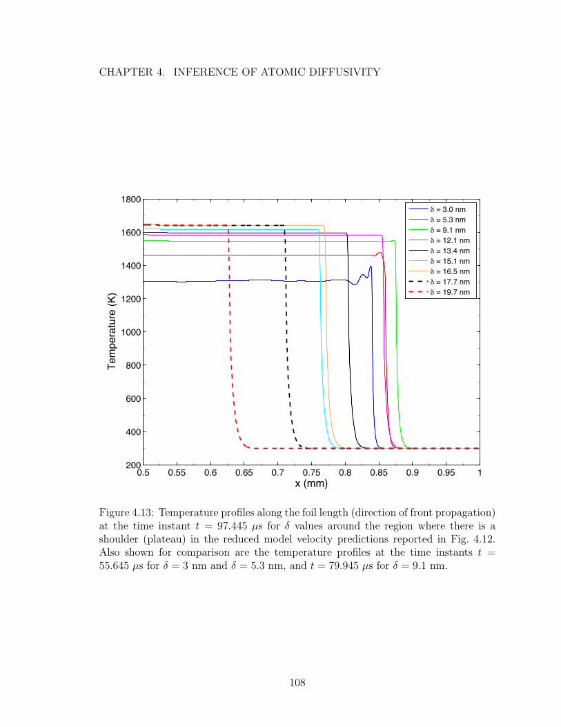
CHAPTER 4. INFERENCE OF ATOMIC DIFFUSIVITY
0.5 0.55 0.6 0.65 0.7 0.75 0.8 0.85 0.9 0.95 1200
400
600
800
1000
1200
1400
1600
1800
x (mm)
Tem
pera
ture
(K
)
δ = 3.0 nm
δ = 5.3 nm
δ = 9.1 nm
δ = 12.1 nm
δ = 13.4 nm
δ = 15.1 nm
δ = 16.5 nm
δ = 17.7 nm
δ = 19.7 nm
Figure 4.13: Temperature profiles along the foil length (direction of front propagation)at the time instant t = 97.445 µs for δ values around the region where there is ashoulder (plateau) in the reduced model velocity predictions reported in Fig. 4.12.Also shown for comparison are the temperature profiles at the time instants t =55.645 µs for δ = 3 nm and δ = 5.3 nm, and t = 79.945 µs for δ = 9.1 nm.
108
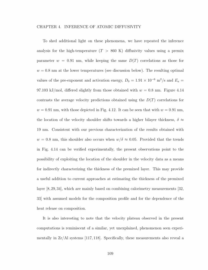
CHAPTER 4. INFERENCE OF ATOMIC DIFFUSIVITY
To shed additional light on these phenomena, we have repeated the inference
analysis for the high-temperature (T > 860 K) diffusivity values using a premix
parameter w = 0.91 nm, while keeping the same D(T ) correlations as those for
w = 0.8 nm at the lower temperatures (see discussion below). The resulting optimal
values of the pre-exponent and activation energy, D0 = 1.91 × 10⁻⁶ m2/s and Ea =
97.103 kJ/mol, differed slightly from those obtained with w = 0.8 nm. Figure 4.14
contrasts the average velocity predictions obtained using the D(T ) correlations for
w = 0.91 nm, with those depicted in Fig. 4.12. It can be seen that with w = 0.91 nm,
the location of the velocity shoulder shifts towards a higher bilayer thickness, δ ≈
19 nm. Consistent with our previous characterization of the results obtained with
w = 0.8 nm, this shoulder also occurs when w/δ ≈ 0.05. Provided that the trends
in Fig. 4.14 can be verified experimentally, the present observations point to the
possibility of exploiting the location of the shoulder in the velocity data as a means
for indirectly characterizing the thickness of the premixed layer. This may provide
a useful addition to current approaches at estimating the thickness of the premixed
layer [8,29,34], which are mainly based on combining calorimetry measurements [32,
33] with assumed models for the composition profile and for the dependence of the
heat release on composition.
It is also interesting to note that the velocity plateau observed in the present
computations is reminiscent of a similar, yet unexplained, phenomenon seen experi-
mentally in Zr/Al systems [117, 118]. Specifically, these measurements also reveal a
109
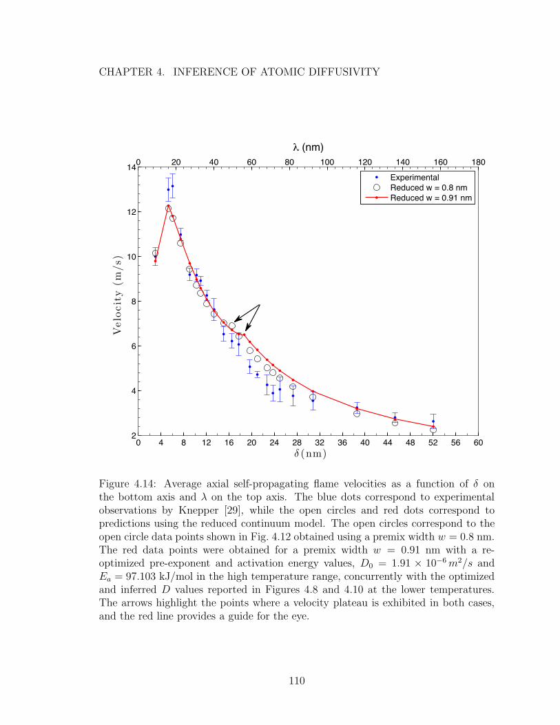
CHAPTER 4. INFERENCE OF ATOMIC DIFFUSIVITY
0 4 8 12 16 20 24 28 32 36 40 44 48 52 56 602
4
6
8
10
12
14
δ (nm)
Velo
cit
y(m
/s)
Experimental
Reduced w = 0.8 nm
Reduced w = 0.91 nm
0 20 40 60 80 100 120 140 160 180
λ (nm)
Figure 4.14: Average axial self-propagating flame velocities as a function of δ onthe bottom axis and λ on the top axis. The blue dots correspond to experimentalobservations by Knepper [29], while the open circles and red dots correspond topredictions using the reduced continuum model. The open circles correspond to theopen circle data points shown in Fig. 4.12 obtained using a premix width w = 0.8 nm.The red data points were obtained for a premix width w = 0.91 nm with a re-optimized pre-exponent and activation energy values, D0 = 1.91 × 10⁻⁶m2/s andEa = 97.103 kJ/mol in the high temperature range, concurrently with the optimizedand inferred D values reported in Figures 4.8 and 4.10 at the lower temperatures.The arrows highlight the points where a velocity plateau is exhibited in both cases,and the red line provides a guide for the eye.
110

CHAPTER 4. INFERENCE OF ATOMIC DIFFUSIVITY
velocity plateau that has a similar structure as that depicted in the inset of Fig. 4.12.
A more elaborate analysis of the underlying causes and influencing factors behind
the predicted Ni/Al velocity plateau, and the possible extensions of such analyses
towards the explanation of the observations in the Zr/Al multilayered systems (see
discussion in [118]) is currently underway, and will be reported as a follow-on work.
4.5 Discussion
Analysis of MD computations and experimental observations of homogeneous and
self-propagating reactions lead to the formulation of a composite D(T ) fit. The lat-
ter is plotted in Fig. 4.15, which also shows estimates of D(T ) that are directly
inferred from MD computations, and the global Arrhenius correlation originally in-
ferred using the analytical model in [42]. As discussed in section 4.4, the composite
fit combines atomic diffusivity estimates inferred from low-temperature ignition ex-
periments, nanocalorimetry experiments, as well as measurements of the velocity of
self-propagating fronts. These respectively yield information regarding the variation
of D at low, intermediate, and high temperatures.
Note that for the present system, the estimates obtained from ignition and nanocalorime-
try are consistent with each other, at least in regions where the corresponding temper-
ature ranges overlap. However, in the composite fit, the diffusivity exhibits a jump as
one moves from the intermediate temperature branch to the high temperature branch.
111
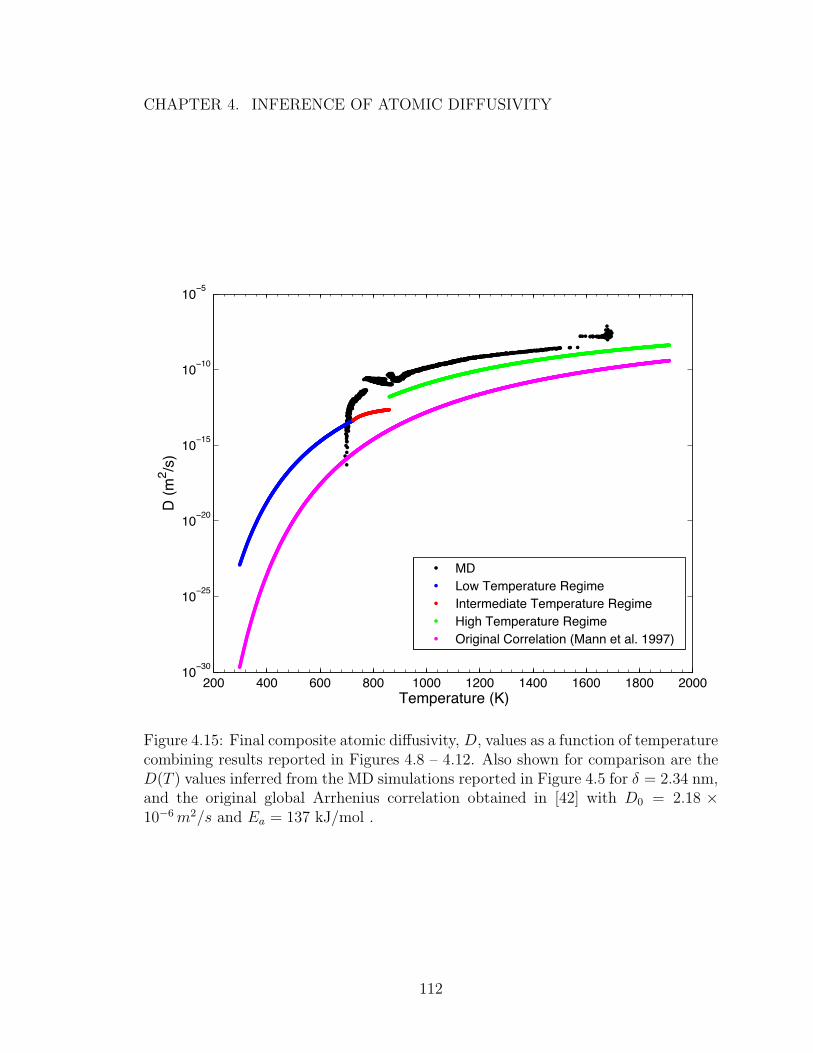
CHAPTER 4. INFERENCE OF ATOMIC DIFFUSIVITY
200 400 600 800 1000 1200 1400 1600 1800 200010
−30
10−25
10−20
10−15
10−10
10−5
Temperature (K)
D (
m2/s
)
MD
Low Temperature Regime
Intermediate Temperature Regime
High Temperature Regime
Original Correlation (Mann et al. 1997)
Figure 4.15: Final composite atomic diffusivity, D, values as a function of temperaturecombining results reported in Figures 4.8 – 4.12. Also shown for comparison are theD(T ) values inferred from the MD simulations reported in Figure 4.5 for δ = 2.34 nm,and the original global Arrhenius correlation obtained in [42] with D0 = 2.18 ×10⁻⁶m2/s and Ea = 137 kJ/mol .
112
CHAPTER 4. INFERENCE OF ATOMIC DIFFUSIVITY
This behavior is in qualitative agreement with observations made in the analysis of
the MD computations. It is interesting to note that in both the MD computations
and the composite fit inferred from macroscale observations, the rapid rise in D oc-
curs near but noticeably below the melting temperature of Al. While the occurrence
of this phenomenon is quite intuitive, additional work is clearly needed in order to
further investigate the underlying microscale mechanisms, and accordingly refine as
appropriate the inferred diffusivity values. Also note that the D(T ) values inferred
from MD are substantially larger than those corresponding to the composite fit. As
mentioned to in section 4.3, the use of diffusivity values directly inferred from MD in
the reduced continuum model would result in large over-estimates of the velocity of
self-propagating fronts. Consequently, additional refinement of the present MD sim-
ulations is clearly needed in order to enable a suitable quantitative characterization
of intermixing rates.
Motivated in large-part by the analysis of the MD predictions, we have relied on
reduced model computations based on a linear dependence of Q on C in the construc-
tion of the composite D(T ) fit. In order to lend further confidence in this approach,
the analysis of section 4.4 was repeated using a quadratic correlation, namely of the
form Q ∝ C2, and the quality of the resulting average self-propagating front velocity
predictions was assessed in terms of their capability to capture the experimental mea-
surements. This assessment (not shown) revealed that using a quadratic correlation
leads to a downward shift of the entire D(T ) composite curve, but unfortunately gave
113
CHAPTER 4. INFERENCE OF ATOMIC DIFFUSIVITY
rise to a larger global error in the average front velocity predictions in comparison
with the linear correlation. This suggests that a linear dependence is the more ap-
propriate form to implement in our reduced model. Nevertheless, despite the present
experience, it would still be worthwhile to explore a more elaborate fit that better ap-
proximates the qualitative trends in MD as well as experimental measurements. This
will be addressed in a follow-on work. In this context, it would also be instructive to
consider a more elaborate thermal model that also accounts for the variation of heat
capacities with temperature.
One should note that the present inference methodology is inherently impacted
by the details of the macroscale descriptions of the prevailing phenomena. Whereas
homogeneous ignition and nanocalorimetry experiments are essentially governed by
local mixing and heat release, self-propagating reaction fronts are in addition gov-
erned by thermal transport along the multilayers. In the present approach, informa-
tion gained from self-propagating reaction fronts is used to infer intermixing rates
at higher temperatures only. This restriction is motivated by the recent observation
in [74] which indicated that for self-propagating reactions evolving adiabatically, most
of the mixing occurs at higher temperatures (T ≥ 1000 K), irrespective of the value
of the bilayer thickness considered (12 nm ≤ δ ≤ 300nm). (The present experiences
are consistent with those in [74], but indicate that for very small δ’s most of the
mixing occurs at T ≥ 900 K). Thus, the velocity of the self-propagating fronts ap-
pears to be weakly sensitive to the details of the mixing rates occurring at the lower
114

CHAPTER 4. INFERENCE OF ATOMIC DIFFUSIVITY
temperatures. A case-in-point is the ability of previous models [31, 41, 42, 47, 76] to
capture the velocity of self-propagating fronts using a global Arrhenius correlation
for D(T ). In this context, the present experiences suggest that these approaches can
be successful in capturing the dynamics of self-propagating fronts while involving, at
the same time, substantial discrepancies in representing intermixing rates prevailing
at low temperatures. This is illustrated in Fig. 4.15, which contrasts the presently
inferred composite D(T ) curve with the original correlation from [42]. Whereas the
original correlation yields lower atomic diffusivity values across the entire temperature
range, largest relative discrepancies are observed at low and intermediate tempera-
tures. Consequently, it appears worthwhile to re-examine, in light of the present
findings, earlier computational attempts at characterizing phenomena that exhibit
high sensitivity to interdiffusion rates at low temperatures, including ignition and
shock initiation. Investigation of these mechanisms is the subject of ongoing work.
Finally, despite the various sources of uncertainty inherent in the various steps of
the analysis, one of the advantages of the present methodology is that the resulting
macroscale representation of interdiffusion rates enables us, for the first time, to
simultaneously capture experimental observations of low-temperature ignition, the
evolution of homogeneous reactions, as well as the velocity of self-propagating fronts.
This motivates further investigation of the validity of the present representations,
namely in order to reduce the impact of these uncertainties and accordingly refine
the model.
115

Chapter 5
Reactive Multilayered Particles
5.1 Motivation
As has been mentioned in the introduction, multilayers were introduced as an
alternative to reactive powders, since they offered a simplified geometry for theoretical
and experimental investigations, allowed for a better control of the reaction properties
and reaction products, and exhibited much faster self-propagating front velocities.
However, certain applications such as chemical time delays [119] or neutralization of
chemical and biological weapons [120], require that the reaction be sustained over long
durations of time or for it to have a small velocity of self-propagation. In powders,
the total reaction time can easily be reduced (though not precisely controlled) by
increasing the porosity and the size of the particles. With multilayers, on the other
hand, this could be achieved either by increasing the bilayer thickness or increasing
116
CHAPTER 5. REACTIVE MULTILAYERED PARTICLES
the foil length. The latter option is usually not practical to fabricate for large-scale
applications, and not suitable for small-scale ones. The former option also has certain
restrictions in that there exists a critical bilayer thickness beyond which rates of heat
losses start overcoming rates of heat generation, eventually causing the reaction to
quench. Consequently, front velocities that are slower than 1 m/s cannot usually be
realized in multilayered foils that are less than 100 µm in thickness.
Realizing that the lower reaction velocities in powders are partly due to the large
thermal contact resistance between the particles, Fritz et al. [121] were able to ex-
ploit this property in order to fabricate compacts of multilayered particles that have
a small propagation velocity. These consisted of NiV/Al layers deposited using DC
magnetron sputtering onto square nylon mesh substrates with 50 µm fiber diameters.
The sputtered multilayered coating was then broken into particles that matched the
size of the mesh elements (each had a width similar to the mesh diameter and were
three times as long) by bending the mesh under water. Loose compacts of these par-
ticles, with a consistent average packing density of 20% of the theoretical maximum
density, were then used in order to measure self-propagating front velocities. Compar-
ing the resulting average velocities in the particle compacts with those in continuous
multilayered foils that have similar average properties (such as bilayer thickness),
Fritz et al. were able to demonstrate that almost a two order of magnitude reduc-
tion in velocity (and as low as approximately 1 cm/s) can be attained using particle
compacts with the given particle dimensions and compact porosity.
117
CHAPTER 5. REACTIVE MULTILAYERED PARTICLES
Motivated by the above experiments, Sraj et al. [122] later extended the transient
reduced numerical model described in section 2.3 of chapter 2, in order to simulate
self-propagating fronts in idealized multilayered particles consisting of quasi-2D rect-
angular foils that are in thermal contact. The Ni/Al multilayered foils were assumed
to be all identical, with a bilayer thickness of λ ≈ 830 nm (δ = 250 nm) and a length
of 1 mm. The thermal conductivity of the foils was assumed to be homogeneous
and equal to the constant average given by Eq. (3.2), while thermal contact between
different particles was established using a reduced thermal conductivity value given
by the sum of the internal foil resistance and a constant thermal contact resistance
value. Moreover, the thermal contact resistance and contact areas were assumed to
be the same for all particles. The model was then used to mainly analyze the depen-
dence of the propagation velocity on the particles’ contact area and thermal contact
resistance. In accordance with the analysis of Fritz, an ignition delay was observed
as the flame crossed from one particle to the next, which consequently resulted in an
overall reduction in the average flame velocity. Furthermore, it was noticed that the
average velocity decreased with an increase in either the contact area (for zero thermal
contact resistance) or the thermal contact resistance (for a given contact area)1, and
that the impact of the thermal contact resistance was mostly prominent for contact
areas < 100 µm. Specifically, average velocity values close to those observed experi-
1Note that, for the case of perfect thermal contact, the velocity curve exhibited a monotonicallydecreasing trend as the contact area was increased. However, when a thermal contact resistancewas introduced, the trend became non-monotonic, starting with an increasing trend at low contactareas, before switching to a decreasing trend for contact areas > 100 µm.
118

CHAPTER 5. REACTIVE MULTILAYERED PARTICLES
mentally were attained at the smallest contact areas (10 µm) when contact resistance
(10−5 m2K/W) was accounted for.
In order to gain a more detailed understanding of the reactions occurring in mul-
tilayered particle compacts and to be able to fully explore their behavior, we need to
move from the idealized scenario presented above to simulating more realistic particle
networks. One drawback, though, is that the quasi-2D computations conducted by
Sraj et al. required a 1 µm discretizing mesh size, resulting in about 104 computa-
tional node points for each particle, which for a 3D model would lead to 107 degrees
of freedom. Moreover, for moderately thick bilayers, a reaction front would need on
the order of a msec in physical time to cross between particles with a computational
time-step of ∼ 10−7 secs. For relatively thin bilayers and large thermal contact re-
sistances, a much smaller time-step on the order of nsecs would be required, namely
to avoid numerical stability issues caused by the sudden discontinuity experienced by
the fast moving fronts at the particle interfaces. The high spatial dimensionality of
the system is further compounded by additional factors such as porosity, connectivity,
particle surface oxidation, thermal contact resistance, contact area, bilayer thickness,
particle size, particle shape, and particle orientation. As a result, using existing mod-
els for simulations of more realistic particle networks that contain at least hundreds
of particles in a 3D configuration could prove to be computationally very costly, if
not prohibitive.
One means of moderating the hurdles above would be to attempt to reduce the
119
CHAPTER 5. REACTIVE MULTILAYERED PARTICLES
dimensionality through spatially homogenizing the system on the level of a single par-
ticle. This would help avert the need to mesh over each particle, and thus bring about
a reduction of almost 4–7 orders of magnitude, in addition to easing the restrictions
on the size of the time-step. However, as with every averaging or filtering approach,
one also runs the risk of grossly misrepresenting the actual reaction dynamics, which
could greatly depend on a proper resolution of the small scales. A common remedy
to this problem is to upscale or coarse-grain the governing system of equations such
that the effects of the unresolved microscales on the macroscale dynamics are prop-
erly accounted for. Another simpler, though more restrictive, approach would be to
numerically identify certain regimes under which such a homogenization would be
valid or applicable. In this chapter, we will adopt this latter approach.
Numerous experimental [123–128] and numerical [128–139] studies have already
been carried out on reaction-diffusion phenomena in heterogeneous media. The ex-
perimental investigations have mainly focused on reactions occurring in either gasless
powder mixtures, or between a powder and a gas. On the other hand, the theoretical
and numerical studies have considered cases where one of the reactants is comprised of
particles or point sources embedded in a homogeneous medium of the other reactant,
or where the medium is composed of discrete reactive cells or point sources contain-
ing the homogeneously fully mixed reactants. Most of these studies have focused on
demonstrating the discrete nature of the reaction, and have tended to emphasize the
invalidity of the homogeneous [140] and the quasi-homogeneous [141] approximations
120

CHAPTER 5. REACTIVE MULTILAYERED PARTICLES
in such situations due to the fact that they fail to correctly capture crucial proper-
ties of the reaction propagation. In the homogeneous approximation, the reaction
kinetics depend only on a uniform distribution of the temperature and concentration
of the reactants, whereas in the quasi-homogeneous approximation, the reaction ki-
netics account for the presence of certain heterogeneities in the system using some
functional form, but are otherwise homogeneous over space. Numerical and analyt-
ical comparisons between the predictions of the discrete and quasi-homogeneous (or
homogeneous) models were examined, and certain criteria for the domains of applica-
bility of the homogenized versions were determined. These criteria are mostly based
on ratios of reaction to diffusion time-scales, ratios of reaction to heat transfer time-
scales, or ratios of length scales given by the front width (reaction and diffusion) to
the particle size or to the characteristic scale of the system’s heterogeneity.
Varma et al. [129], for instance, considered a solid-gas system of Ti-N2, which they
modeled as set of identical 2D square reaction cells with blunt edges, arranged in a
random fashion on a square lattice with a prescribed degree of porosity. Each reaction
cell contained both reactants in a fully pre-mixed state, and was in contact with its
nearest neighbors on the lattice along the flat edges (that is with a contact area
equal to half the cell’s diameter). The cells were also assumed to be immersed in a
homogeneous gaseous medium, and that both (the cells and the medium) had constant
thermo-physical properties, including a constant thermal contact resistance value at
the interface between two contacting cells. The domain was then discretized using a
121

CHAPTER 5. REACTIVE MULTILAYERED PARTICLES
square mesh with a size equal to half the reaction cell’s diameter, and used to solve
the coupled system of differential equations for the evolutions of temperature (melting
was not taken into account) and concentration. Only heat transfer by conduction was
considered and an effective constant thermal conductivity value, composed of a sum
of resistances in series/parallel, was used for calculating the heat fluxes. The reaction
rate was assumed to be zero below a certain fixed ignition temperature, beyond which
it proceeds at a constant fixed rate until all the reactants are consumed. A systematic
study was then conducted, analyzing the dependence of the reaction front structure
and velocity on the particle size and density. Based on these results, a parametric
map of density vs. particle size was constructed, outlining the regions of transition
between quasi-homogeneous, relay-race2, and percolation regimes. Their observations
led them to conclude that the main criterion which determines the transition between
the continuum and the discrete limit is the ratio of the reaction to the heat transfer
(or heat conduction) time-scales. Specifically, they argue [125, 128] that if trxn ≫
tconduction, then the reaction (and thermal) front would encompass several particles
such that the continuum approximation becomes justified, whereas in the opposite
limit, the width of the reaction front becomes comparable to the size of a single
particle which consequently necessitates a discrete representation of the dynamics.
Another study, based on a more basic model than that of Varma et al., was
conducted by Rogachev [130]. A quasi-1D linear chain of reaction cells was considered,
2Relay-race regime is described as a series of localized successive, but intermittent, rapid ignitions,separated by long induction (or heating) periods in between each ignition event.
122
CHAPTER 5. REACTIVE MULTILAYERED PARTICLES
with each cell containing both reactants in a fully mixed state. Melting events were
not taken into account, and heat transfer by conduction occurred between the reaction
cells only, while all other forms of heat transfer were ignored. The temperature inside
each cell was assumed to be uniform (i.e. temperature gradients were ignored) on
the basis that the internal thermal resistance of the solid (or reaction cell) is much
lower than the thermal contact resistance between two contacting cells. Thus, each
reaction cell was characterized by a temperature value and a degree of conversion
(or concentration) value, with the rate of heat conduction between touching cells
being proportional to the product of the temperature difference between the cells, a
fixed contact area, and fixed heat transfer coefficient. Contrary to Varma though, two
forms of the reaction rate were considered; both exhibited an Arrhenius dependence on
temperature, but one in a continuous fashion over all temperatures, and the other in a
step-like fashion such that the rate was zero below a certain ignition temperature, and
Arrhenius beyond that. The time evolutions of temperature, concentration, reaction
rate, and front velocity were analyzed as a function of a parameter representing
the ratio of the characteristic time-scales of heat transfer to reaction rate. Velocity
predictions of the numerical model for different values of the parameter were compared
to those given by Zeldovich’s analytical expression for the velocity, derived using the
homogeneous (continuum) medium approximation. It was noticed that deviations
from the homogeneous predictions became more prominent with increasing values
of the ratio of heat transfer time to reaction time, and that the propagation regime
123

CHAPTER 5. REACTIVE MULTILAYERED PARTICLES
depended on this ratio, along with the sensitivity of the reaction rate to the initial and
combustion (or flame) temperatures. Moreover, it was seen that for strongly activated
reactions, the front velocity is independent of the imposed ignition temperature (in
the step-wise reaction kinetics case) below a certain critical ignition value, whereas
a universal dependence was exhibited for ignition temperatures above this critical
value.
The conclusions arrived at by the above two investigations, which help sum up the
main viewpoints of most of the other studies referenced earlier, seem to emphasize
the fact that the prime factor in determining the validity of a spatially homogenized
medium concerns the ratio of the reaction time scale to the heat transfer time scale.
At first glance, it might seem as though this could also serve as the governing criterion
in our case as to whether or not we can safely spatially homogenize our system on
the level of a single particle. However, the previous approaches impose a number of
simplifying assumptions that are inconsistent with our model, and this renders their
established criterion not directly applicable to our multilayered particles, but rather
entails its re-examination for our specific case.
One source of incompatibility lies in the fact that both Rogachev and Varma
considered particles in which the reactants were initially present in a homogeneously
premixed state, thus atomic diffusion was not present as a limiting factor in their
reaction rate expressions. This is a major inconsistency with the case that we are
interested in, since the reactants in our particles exist initially as separate alternating
124
CHAPTER 5. REACTIVE MULTILAYERED PARTICLES
layers and we assume that the reaction rate is diffusion rather than reaction-limited.
In the case of Varma, the reaction was assumed to initiate at a specific ignition
temperature, after which it proceeds at a constant rate. Defining a fixed ignition
temperature value for the reaction cannot be accomplished in a unique manner and
is usually mostly appropriate for high activation energies, which is not a necessary
condition for us in view of the results presented in chapter 4. Whereas assuming
a constant reaction rate is synonymous to assuming that the reaction occurs under
isothermal conditions, and this seems to be at odds even with the conditions in
Varma’s study. In the case of Rogachev, an Arrhenius dependence on temperature was
assumed, but with the use of a single value for the activation energy and the diffusion
coefficient. This does not comply with our observations in chapter 4, specifically
when melting and intermediate phase formation events take place. Furthermore,
Rogachev did not include a dependence of the reaction rate on the degree of reactant
consumption, but rather imposed an abrupt discontinuous termination of the reaction.
This is particularly inconsistent with compacts comprised of layered particles.
While Varma and Rogachev, along with most of the other studies, undertook the
problem of characterizing the reaction’s heterogeneity on scales on the order of a
particle size, they ignored taking into account heterogeneities on scales smaller than
this, mainly based on the fact that the thermal resistance in the particle’s interior
is much lower than that across the contact interface. For self-propagating reactions,
especially those that take place in multilayered structures, such an assumption is not
125

CHAPTER 5. REACTIVE MULTILAYERED PARTICLES
always obvious, and in fact has clearly been shown to be violated for the particle sizes
examined by Sraj et al. [122]. Moreover, thermal diffusion effects within a particle
(which is different from thermal diffusion between particles) could have important
ramifications on the flame front macroscale dynamics (such as stability) as has already
been demonstrated in chapter 3. We should note though, that an exception was a
study conducted by Grinchuk et al. [138], who did consider thermal diffusion within
the particles, but apart from this, their study still suffers from some of the other
drawbacks and inconsistencies listed above.
A final point worth noting is that the criterion, put forward by the above men-
tioned works, is namely based on a comparison between the chemical reaction and
heat transfer time-scales. Whereas the latter time scale can easily be estimated a
priori, the reaction time-scale is, in most circumstances, difficult to represent using
a single constant value. This is due to the obvious fact that the reaction rate has a
non-trivial dependence on temperature, and in the case of multilayers, on the bilayer
thickness as well. As a result, the comparison cannot readily be employed as a bench-
mark for checking the validity of spatial homogenization in the presently considered
reactive media.
Given all of the above shortcomings, it seems reasonable to re-address the issue
of identifying the regimes under which a homogeneous particle approximation holds,
within the specific context, conditions, and assumptions of our fully generalized re-
duced reaction model presented in chapter 4.
126
CHAPTER 5. REACTIVE MULTILAYERED PARTICLES
5.2 Problem Formulation and Approach
We will start from the generalized reduced model presented in the previous chap-
ter, which consists of the following two coupled system of differential equations:
∂τ
∂t=
D(T )
δ2(5.1)
∂H
∂t= − 1
V
∫
V
(∇ · q)dV +∂Q
∂t(5.2)
where D(T ) is given by the composite fit inferred in chapter 4 (see Fig. 4.15). In
accordance with the observations and analysis of the pervious chapter, we will use a
linear dependence of the reaction heat on the mean concentration such that:
∂Q
∂t= −ρcp∆Tf
∂C(t)
∂t(5.3)
As has been remarked previously, the temperature, T , can be retrieved from the
volume-averaged enthalpy, H , by inverting the complex relationship (2.8) involving
the heats of fusion of the reactants and products [76].
Since the experimentally manufactured multilayered particles [121] consist of NiV/Al
layers, we will account for the presence of Vanadium through estimating ∆Tf based
on the experimentally measured reaction heat [29, 100], namely ∆Hrxn = 1200 J/g.
The heat flux, q, is again assumed to follow Fourier’s law. We will rely on the fully
generalized thermal transport model derived in chapter 3, which corresponds to an
anisotropic, concentration-dependent, and temperature-dependent thermal conduc-
tivity, κ, that also appropriately accounts for the presence of Vanadium.
127

CHAPTER 5. REACTIVE MULTILAYERED PARTICLES
As has been mentioned above, our aim is to extend this modeling formalism for
single multilayers towards exploring reactions occurring in layered particle networks.
However, because of the high dimensionality and the high computational costs associ-
ated with simulating such systems, we will attempt to further reduce the generalized
reduced model through imposing spatial homogenization on the level of a single par-
ticle, and to numerically identify the regimes under which such a homogenization
would be valid or applicable.
In our homogeneous scenario, particles have spatially uniform temperature and
concentration fields. Accordingly, we can set ∇ · q to zero and the governing system
of equations for a single multilayered particle becomes:
∂τ
∂t=
D(T )
δ2(5.4)
∂H
∂t=
∂Q
∂t= −ρcp∆Tf
∂C(t)
∂t(5.5)
Note that while Eqs. (5.1)–(5.3) correspond to evolution equations within each com-
putational cell of a single meshed multilayered particle, Eqs. (5.4)–(5.5) represent
evolution equations over the entire homogenized particle. Numerical solution of the
system of Eqs. (5.1)–(5.3) is conducted using the same scheme described in section 2.4
of chapter 2. The same technique is implemented for solving Eqs. (5.4)–(5.5), but
with each particle being the equivalent of a single computational cell.
Generalizing the above reduced meshed and homogeneous models to multiple par-
ticles, involves simply applying the same set of equations to each particle separately.
128

CHAPTER 5. REACTIVE MULTILAYERED PARTICLES
Following Sraj et al. [122], coupling between the particles is achieved through ther-
mal conduction between touching particles across a certain surface contact area. In
the meshed case, accounting for heat transfer across particle interfaces occurs via the
heat flux, q, but with a reduced κ value given by the sum of the internal particle
resistance (varies with time) near the interface and a specified (constant) thermal
contact resistance value, Rc. In the homogeneous case, the particles’ internal thermal
resistance is ignored and the heat flux includes only the thermal contact resistance,
Rc.
As we pointed out earlier, the high spatial dimensionality of systems involving mul-
tilayered particle networks is compounded by other complexities arising from factors
such as porosity, connectivity, particle surface oxidation, thermal contact resistance,
contact area, bilayer thickness, particle size, particle shape, and particle orientation,
in addition to the potential presence of variability in all of these properties. Thus,
to render the problem manageable, we introduce a number of simplifications by elim-
inating some of these sources of complexity. Specifically, we focus on an idealized
setup where we have a quasi-1D linear chain of rectangular multilayered particles
that are in full contact. Moreover, apart from heat transfer across the particles’ sur-
face contact areas, we assume that the reactions occur under adiabatic conditions.
This is in accordance with the vacuum conditions under which the experimental ve-
locity measurements are typically conducted, and the negligible effects of radiative
heat losses (for thick samples [46]). We also impose the condition that the first par-
129
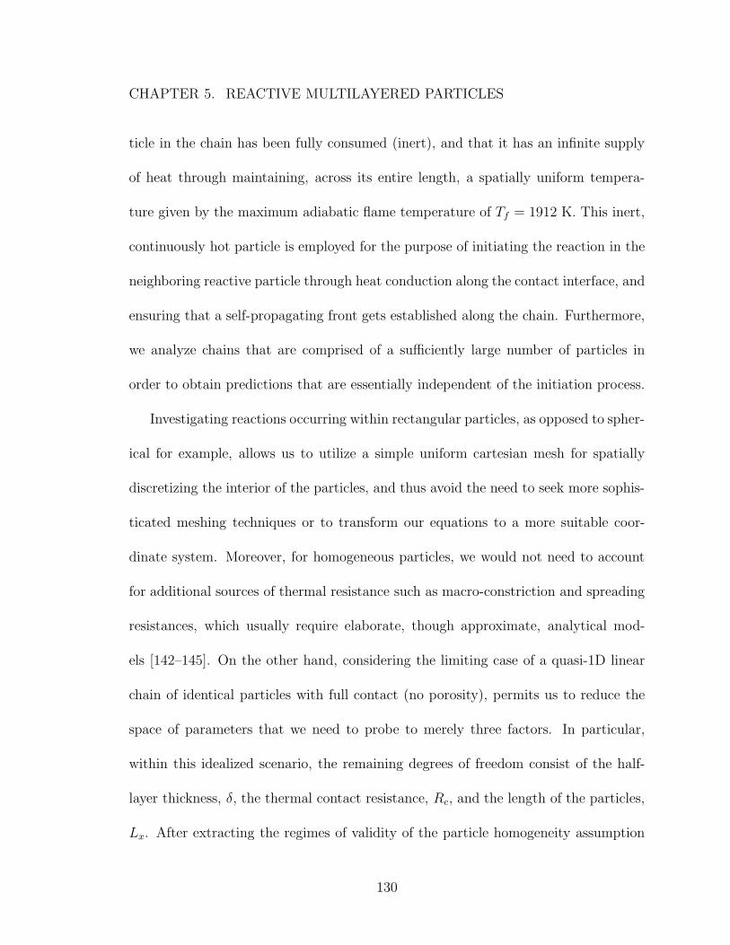
CHAPTER 5. REACTIVE MULTILAYERED PARTICLES
ticle in the chain has been fully consumed (inert), and that it has an infinite supply
of heat through maintaining, across its entire length, a spatially uniform tempera-
ture given by the maximum adiabatic flame temperature of Tf = 1912 K. This inert,
continuously hot particle is employed for the purpose of initiating the reaction in the
neighboring reactive particle through heat conduction along the contact interface, and
ensuring that a self-propagating front gets established along the chain. Furthermore,
we analyze chains that are comprised of a sufficiently large number of particles in
order to obtain predictions that are essentially independent of the initiation process.
Investigating reactions occurring within rectangular particles, as opposed to spher-
ical for example, allows us to utilize a simple uniform cartesian mesh for spatially
discretizing the interior of the particles, and thus avoid the need to seek more sophis-
ticated meshing techniques or to transform our equations to a more suitable coor-
dinate system. Moreover, for homogeneous particles, we would not need to account
for additional sources of thermal resistance such as macro-constriction and spreading
resistances, which usually require elaborate, though approximate, analytical mod-
els [142–145]. On the other hand, considering the limiting case of a quasi-1D linear
chain of identical particles with full contact (no porosity), permits us to reduce the
space of parameters that we need to probe to merely three factors. In particular,
within this idealized scenario, the remaining degrees of freedom consist of the half-
layer thickness, δ, the thermal contact resistance, Rc, and the length of the particles,
Lx. After extracting the regimes of validity of the particle homogeneity assumption
130
CHAPTER 5. REACTIVE MULTILAYERED PARTICLES
as a function of these three parameters, or possibly in terms of some reduced di-
mensionless combination of them, the other parameters can later be systematically
introduced and their effects on the robustness of the predictions can be examined.
131
CHAPTER 5. REACTIVE MULTILAYERED PARTICLES
5.3 Results
In this section, we perform a comparative analysis between the meshed and
homogeneous computations in order to identify the regimes under which the ho-
mogeneous particle approximation is appropriate. Specifically, we seek to deter-
mine when we can safely replace the meshed system of equations (5.1)–(5.2) with
the particle homogenized equations (5.4)–(5.5), without sacrificing the fidelity of
the computational predictions regarding the macroscale reaction dynamics occur-
ring on scales ≥ to the size of a particle. As described in the previous section,
computations are conducted for a quasi-1D linear chain of rectangular multilay-
ered particles, in full contact, with different values of thermal contact resistance
Rc = 10−7; 3 × 10⁻⁷; 7 × 10⁻⁷; 10−6; 3 × 10⁻⁶; 7 × 10⁻⁶ and 10−5 m2K/W , particle
length L = 10; 50; 100 and 500 µm, and bilayer thickness corresponding to δ = 50
and 250 nm. Note that the values of Rc and L that we consider in this study, even
though not exhaustive, help span a wide range of possible (analytically estimated)
values that could typically be encountered in real contacting particles [143–145].
In the meshed scenario, each particle is described using the state vector(
C(x, t, n), T (x, t, n))
,
where x, t, and n represent position in the x-direction, time, and particle (ID) number
respectively, whereas in the homogeneous scenario, each particle is instead described
using the state vector(
C(t, n), T (t, n))
. Because we aim at being able to replace the
former description with the latter, we expect this approximation to become asymp-
totically valid as we approach the limit of vanishing temperature gradients within a
132

CHAPTER 5. REACTIVE MULTILAYERED PARTICLES
single particle. Therefore, we start first by characterizing the degree of temperature
heterogeneity in the particles using the meshed computations to see whether we can
identify some critical range or combination of Rc, δ, and L, where the temperature
variations in the interior of the particles become negligible. For this purpose, we de-
fine two measures that reflect the extent of temperature gradients within a particle,
given by:
Smax =max { Tmax(t, n)− Tmin(t, n) }
Tf − T0
(5.6)
< S(t) >=< Tmax(t, n)− Tmin(t, n) >t
Tf − T0(5.7)
where Tf and T0 refer to the adiabatic flame temperature and room (initial) tem-
perature, respectively. Expression (5.6) corresponds to the normalized peak value
of the instantaneous maximum temperature difference in a given particle, whereas
expression (5.7) corresponds to the normalized time average of Smax(t). Smax and
< S(t) > are calculated for each particle in the chain, but in our analysis we rely only
on values from particles that are appreciably away from the domain boundaries. In
all of the cases that we have analyzed, these measures become almost constant near
the center of the chain, so in our results we only report the values that correspond to
particles situated at the chain’s midpoint. Note also that, in order to avoid biasing
< S(t) > to low values, S(t) for a given particle is averaged between the times when
the reaction is about to transfer to and from the particle of interest.
133

CHAPTER 5. REACTIVE MULTILAYERED PARTICLES
Figures (5.1) and (5.2) show Smax and < S(t) > as a function of Rc, plotted
for different values of L and δ. It can be noticed that, for a given δ value, both
measures exhibit an overall decrease with increasing values of Rc and decreasing
values of L. This is consistent with the fact that as the thermal contact resistance
increases, the rate of thermal conduction between different particles decreases, thus
allowing more time for heat within the particles to diffuse and smoothen out the
temperature gradients. Meanwhile, for a fixed Rc, the time required for the particles
to achieve a homogeneous temperature state decreases as L decreases, causing shorter
particles to admit lower temperature gradients than longer ones. Note that Smax helps
us to quantify the maximum possible instantaneous temperature difference that can
occur within a particle for the given conditions. This mostly takes place during front
formation and propagation in the interior of the particle, provided that the particle
is long enough for a (strong) front to get established. Increasing Rc helps decrease
the maximum temperatures attained in the flame, but up to a limited extent. This
explains why Smax eventually seems to asymptote as a function of Rc. Moreover
as has been demonstrated in chapter 3, since the reaction rate in multilayers with
δ = 250 nm is slower, and thus has a larger thermal (and reaction) width than
δ = 50 nm, Smax is smaller for the former than the latter for a given L value. The
small kinks that appear in the curves in Fig. (5.1) are due to the different time instants
at which this maximum temperature difference occurs. For example, for δ = 250 nm,
L = 100 µm, and Rc = 3 × 10⁻⁷ m2K/W, the maximum occurs during the early
134

CHAPTER 5. REACTIVE MULTILAYERED PARTICLES
heating stages of the particle (just before a front initiates) when heat has not yet had
enough time to diffuse to the neighboring cold regions of the particle, whereas for
Rc = 7 × 10⁻⁷ m2K/W, it occurs when the front initiates. In the former case, there
is usually a slight back-flow of heat into the previous reacted particle as soon as the
front initiates due to the small Rc value, and this causes the temperature gradients
to be maximized just before the front has fully initiated and not after. Such a slight
increase in Smax with Rc happens only for certain combinations of Rc, L, and δ, and
so is not observed in all of the curves in Fig. (5.1).
On the other hand, < S(t) > is more representative of the overall average range of
instantaneous temperature gradients that occur within a certain particle around the
time of its reaction, and emphasizes more the gradients that are sustained for longer
periods of times. Consequently, it exhibits lower values than Smax, is monotonic
as a function of Rc (no kinks), and asymptotes to much lower values at high Rc.
Furthermore, the curves for the two different δ’s almost overlap, with deviations
between the two becoming more noticeable as L increases. Since δ = 250 nm has a
lower propagation velocity than δ = 50 nm, larger gradients are sustained for longer
times in thicker multilayers and sufficiently long particles. Note however, that for
small L and Rc values, δ = 250 nm has lower < S(t) > values, again due to the
slower reaction rates and larger thermal and reaction widths.
135

CHAPTER 5. REACTIVE MULTILAYERED PARTICLES
0 10 20 30 40 50 60 70 80 90 1000
0.1
0.2
0.3
0.4
0.5
0.6
0.7
0.8
0.9
1
Rc × 10−7 (m2K/W )
Sm
ax
δ = 50 nm; L = 10µm L = 50 L = 100 L = 500 δ = 250 nm; L = 10µm
Figure 5.1: Normalized peak values of the instantaneous maximum and minimumtemperature differences in a given particle, Smax, as a function of thermal contactresistance Rc. Plotted are curves corresponding to different values of particle size, L,and half-layer thickness, δ. Solid lines with solid dots correspond to δ = 50 nm, whiledashed lines with open circles correspond to δ = 250 nm.
136
CHAPTER 5. REACTIVE MULTILAYERED PARTICLES
0 10 20 30 40 50 60 70 80 90 1000
0.1
0.2
0.3
0.4
0.5
0.6
0.7
Rc × 10−7 (m2K/W )
<S
(t)
>
δ = 50 nm; L = 10µm
L = 50
L = 100
L = 500
δ = 250 nm; L = 10µm
Figure 5.2: Normalized time average of the instantaneous maximum and minimumtemperature differences in a given particle, < S(t) >, as a function of thermal contactresistance Rc. Plotted are curves corresponding to different values of particle size, L,and half-layer thickness, δ. Solid lines with solid dots correspond to δ = 50 nm, whiledashed lines with open circles correspond to δ = 250 nm.
137

CHAPTER 5. REACTIVE MULTILAYERED PARTICLES
Considering that short-lived, large temperature variations in the particles might
not have a substantial impact on the macroscale (scales ≥ L) reaction propagation,
we expect the < S(t) > measure to be a more suitable indicator of the actual degree
of temperature heterogeneity within the particles for a given set of parameters. Thus
by examining Fig. (5.2), we postulate that particles with δ ≥ 50 nm, L ≤ 100 µm,
and Rc ≥ 30×10−7 m2K/W can be considered to be fairly homogeneous and that for
such particles, we might be able to safely replace the meshed set of equations with
the homogenized set of equations for a more suitable but still reliable description
of the reaction dynamics. Note however, that the restriction to high Rc values for
ensuring temperature homogeneity can be successively relaxed for shorter particles
(L < 100 µm), while still maintaining small errors.
In order to check our postulation, we need to quantify and characterize the error
associated with using the approximate homogeneous particle equations instead of the
meshed system of equations for describing the reaction progress between the particles.
For this purpose, we define a relative time error measure given by:
terror =tmeshed − thomogeneous
tmeshed
(5.8)
where t corresponds to the time that has passed between when 70% of the previous
particle in the chain has been consumed and when the current particle of interest has
reached a 70% consumption level, while the subscripts correspond to the meshed and
homogenized particles respectively. Similar to the heterogeneity measures above, in
our analysis we rely only on t values from particles that are appreciably away from
138
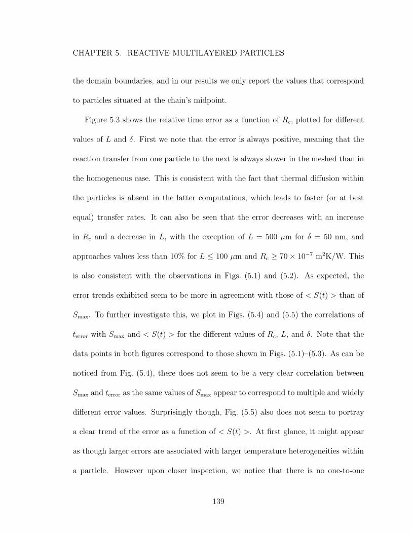
CHAPTER 5. REACTIVE MULTILAYERED PARTICLES
the domain boundaries, and in our results we only report the values that correspond
to particles situated at the chain’s midpoint.
Figure 5.3 shows the relative time error as a function of Rc, plotted for different
values of L and δ. First we note that the error is always positive, meaning that the
reaction transfer from one particle to the next is always slower in the meshed than in
the homogeneous case. This is consistent with the fact that thermal diffusion within
the particles is absent in the latter computations, which leads to faster (or at best
equal) transfer rates. It can also be seen that the error decreases with an increase
in Rc and a decrease in L, with the exception of L = 500 µm for δ = 50 nm, and
approaches values less than 10% for L ≤ 100 µm and Rc ≥ 70× 10−7 m2K/W. This
is also consistent with the observations in Figs. (5.1) and (5.2). As expected, the
error trends exhibited seem to be more in agreement with those of < S(t) > than of
Smax. To further investigate this, we plot in Figs. (5.4) and (5.5) the correlations of
terror with Smax and < S(t) > for the different values of Rc, L, and δ. Note that the
data points in both figures correspond to those shown in Figs. (5.1)–(5.3). As can be
noticed from Fig. (5.4), there does not seem to be a very clear correlation between
Smax and terror as the same values of Smax appear to correspond to multiple and widely
different error values. Surprisingly though, Fig. (5.5) also does not seem to portray
a clear trend of the error as a function of < S(t) >. At first glance, it might appear
as though larger errors are associated with larger temperature heterogeneities within
a particle. However upon closer inspection, we notice that there is no one-to-one
139
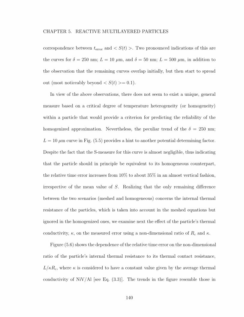
CHAPTER 5. REACTIVE MULTILAYERED PARTICLES
correspondence between terror and < S(t) >. Two pronounced indications of this are
the curves for δ = 250 nm; L = 10 µm, and δ = 50 nm; L = 500 µm, in addition to
the observation that the remaining curves overlap initially, but then start to spread
out (most noticeably beyond < S(t) >= 0.1).
In view of the above observations, there does not seem to exist a unique, general
measure based on a critical degree of temperature heterogeneity (or homogeneity)
within a particle that would provide a criterion for predicting the reliability of the
homogenized approximation. Nevertheless, the peculiar trend of the δ = 250 nm;
L = 10 µm curve in Fig. (5.5) provides a hint to another potential determining factor.
Despite the fact that the S-measure for this curve is almost negligible, thus indicating
that the particle should in principle be equivalent to its homogeneous counterpart,
the relative time error increases from 10% to about 35% in an almost vertical fashion,
irrespective of the mean value of S. Realizing that the only remaining difference
between the two scenarios (meshed and homogeneous) concerns the internal thermal
resistance of the particles, which is taken into account in the meshed equations but
ignored in the homogenized ones, we examine next the effect of the particle’s thermal
conductivity, κ, on the measured error using a non-dimensional ratio of Rc and κ.
Figure (5.6) shows the dependence of the relative time error on the non-dimensional
ratio of the particle’s internal thermal resistance to its thermal contact resistance,
L/κRc, where κ is considered to have a constant value given by the average thermal
conductivity of NiV/Al [see Eq. (3.3)]. The trends in the figure resemble those in
140
CHAPTER 5. REACTIVE MULTILAYERED PARTICLES
0 10 20 30 40 50 60 70 80 90 1000
0.1
0.2
0.3
0.4
0.5
0.6
0.7
0.8
0.9
Rc × 10−7 (m2K/W )
t error
δ = 50 nm; L = 10µm L = 50 L = 100 L = 500 δ = 250 nm; L = 10µm
100
101
102
10−2
10−1
100
Figure 5.3: Relative time error in the reaction progress between the meshed andhomogeneous computations as a function of thermal contact resistance Rc. Plottedare curves corresponding to different values of particle size, L, and half-layer thickness,δ. Solid lines with solid dots correspond to δ = 50 nm, while dashed lines with opencircles correspond to δ = 250 nm. Inset shows the same data points plotted on alog-log scale.
141

CHAPTER 5. REACTIVE MULTILAYERED PARTICLES
0 0.1 0.2 0.3 0.4 0.5 0.6 0.7 0.8 0.9 10
0.1
0.2
0.3
0.4
0.5
0.6
0.7
0.8
0.9
Smax
terror
δ = 50 nm; L = 10µm
L = 50
L = 100
L = 500
δ = 250 nm; L = 10µm
Figure 5.4: Relative time error in the reaction progress between the meshed andhomogeneous computations as a function of Smax. Shown are curves corresponding todifferent values of L, Rc, and δ. Solid lines with solid dots correspond to δ = 50 nm,while dashed lines with open circles correspond to δ = 250 nm. Both sets of datapoints correspond to those shown in Figs. (5.1) and (5.3).
142
CHAPTER 5. REACTIVE MULTILAYERED PARTICLES
0 0.1 0.2 0.3 0.4 0.5 0.6 0.70
0.1
0.2
0.3
0.4
0.5
0.6
0.7
0.8
0.9
< S (t ) >
terror
δ = 50 nm; L = 10µm
L = 50
L = 100
L = 500
δ = 250 nm; L = 10µm
Figure 5.5: Relative time error in the reaction progress between the meshed and ho-mogeneous computations as a function of < S(t) >. Shown are curves correspondingto different values of L, Rc, and δ. Solid lines with solid dots correspond to δ = 50 nm,while dashed lines with open circles correspond to δ = 250 nm. Both sets of datapoints correspond to those shown in Figs. (5.2) and (5.3).
143
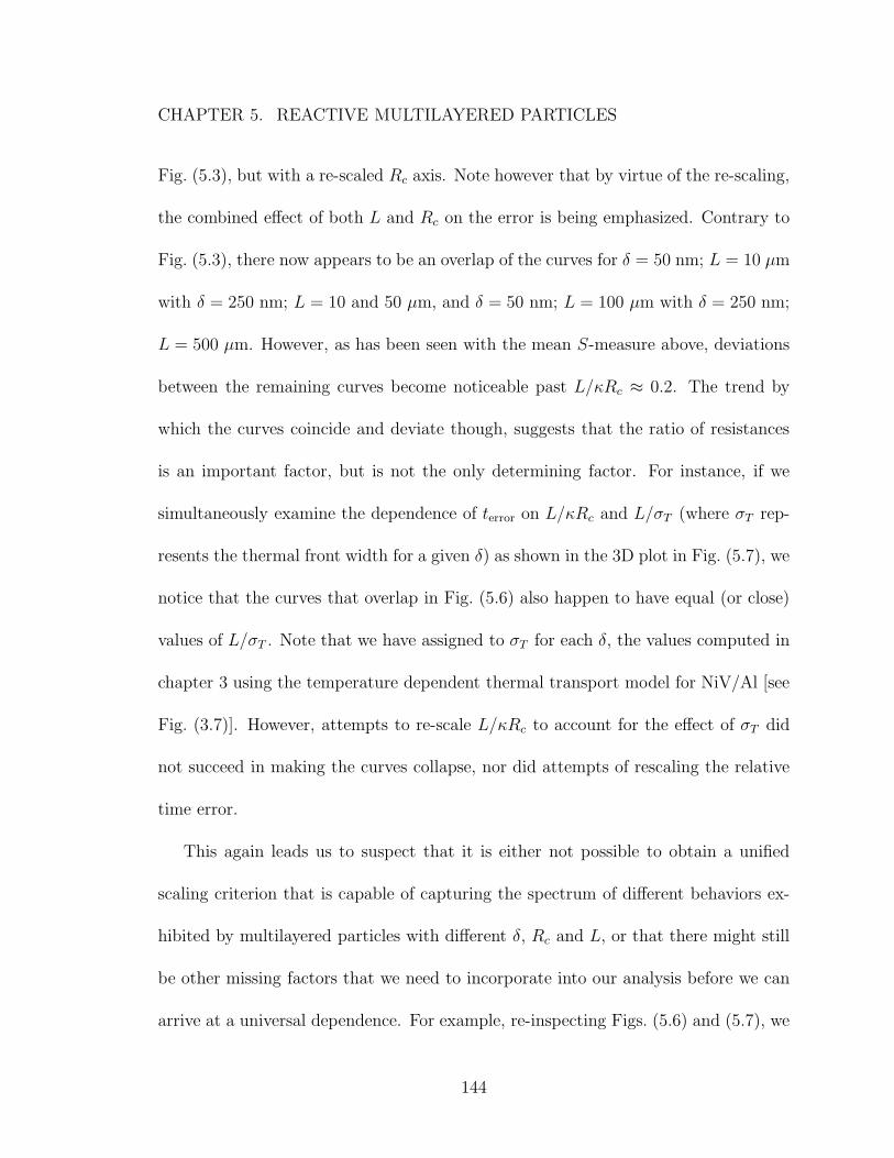
CHAPTER 5. REACTIVE MULTILAYERED PARTICLES
Fig. (5.3), but with a re-scaled Rc axis. Note however that by virtue of the re-scaling,
the combined effect of both L and Rc on the error is being emphasized. Contrary to
Fig. (5.3), there now appears to be an overlap of the curves for δ = 50 nm; L = 10 µm
with δ = 250 nm; L = 10 and 50 µm, and δ = 50 nm; L = 100 µm with δ = 250 nm;
L = 500 µm. However, as has been seen with the mean S-measure above, deviations
between the remaining curves become noticeable past L/κRc ≈ 0.2. The trend by
which the curves coincide and deviate though, suggests that the ratio of resistances
is an important factor, but is not the only determining factor. For instance, if we
simultaneously examine the dependence of terror on L/κRc and L/σT (where σT rep-
resents the thermal front width for a given δ) as shown in the 3D plot in Fig. (5.7), we
notice that the curves that overlap in Fig. (5.6) also happen to have equal (or close)
values of L/σT . Note that we have assigned to σT for each δ, the values computed in
chapter 3 using the temperature dependent thermal transport model for NiV/Al [see
Fig. (3.7)]. However, attempts to re-scale L/κRc to account for the effect of σT did
not succeed in making the curves collapse, nor did attempts of rescaling the relative
time error.
This again leads us to suspect that it is either not possible to obtain a unified
scaling criterion that is capable of capturing the spectrum of different behaviors ex-
hibited by multilayered particles with different δ, Rc and L, or that there might still
be other missing factors that we need to incorporate into our analysis before we can
arrive at a universal dependence. For example, re-inspecting Figs. (5.6) and (5.7), we
144

CHAPTER 5. REACTIVE MULTILAYERED PARTICLES
0 5 10 15 20 25 30 350
0.1
0.2
0.3
0.4
0.5
0.6
0.7
0.8
0.9
L/kRc
t error
δ = 50 nm; L = 10µm
L = 50
L = 100
L = 500
δ = 250 nm; L = 10µm
0 0.2 0.5 1 1.5 20
0.1
0.2
0.3
0.4
Figure 5.6: Relative time error, terror, as a function of the non-dimensional ratio ofthe particle’s internal thermal resistance, L/κ, to its thermal contact resistance, Rc.Shown are curves corresponding to different values of L, Rc, and δ. Solid lines withsolid dots correspond to δ = 50 nm, while dashed lines with open circles correspondto δ = 250 nm. Inset provides a close-up into the region of small error and high Rc
values.
145

CHAPTER 5. REACTIVE MULTILAYERED PARTICLES
05
1015
2025
0
10
20
30
40
0
0.1
0.2
0.3
0.4
0.5
0.6
0.7
0.8
0.9
L/σTL/kRc
t error
Figure 5.7: 3D plot of terror as a function of L/κRc and the non-dimensional ratioof particle size to thermal front width, L/σT . Shown are curves corresponding todifferent values of L, Rc, and δ. Solid lines with solid dots correspond to δ = 50 nm,while dashed lines with open circles correspond to δ = 250 nm. σT = 100 µm forδ = 250 nm and 20 µm for δ = 50 nm. The terror 2D slice helps highlight the pointsat which the curves cross the 10% error threshold.
146

CHAPTER 5. REACTIVE MULTILAYERED PARTICLES
see that while particles with similar ratios of L/σT tend to have similar sensitivities of
the error on L/κRc, particles with larger ratios give rise to lower sensitivities (smaller
errors). This observation runs counter to what we might have expected, since the
smaller the size of the particles is, compared to the thermal front width associated
with the layering, the more homogeneous their interior temperature fields would be
and thus should relate more closely with the homogeneous reaction description. It
is possible that for long particles (such as L = 500 µm), the dominating factor is no
longer the ratio of internal to contact thermal resistance, but rather the velocity of
front propagation (which is a function of reaction rate and the internal thermal resis-
tance) in the meshed particles, compared to the rates of reaction and heat conduction
in the homogeneous particles. Thus in this scenario, particles that are sufficiently long
and can support a self-propagating front obey a set of criteria that are slightly dif-
ferent than those for shorter particles. This might explain why the relative error for
the case of δ = 50 nm; L = 500 µm exhibits an anomalous trend in Fig. (5.3), as
it has a ratio of L/σT that is much larger than all the other curves (see Fig. (5.7))
and by this, it could have already crossed into a regime that is governed by a slightly
different set of criteria than the others. However, it is not directly obvious as to how
one could rescale the relative error using all the various independent parameters that
it depends on, and in a manner such that the effects of each on the error become
more/less prominent at distinct times.
Despite all of the above shortcomings and drawbacks, we were nevertheless success-
147
CHAPTER 5. REACTIVE MULTILAYERED PARTICLES
ful in determining one regime under which the homogeneous particle approximation
would be valid. In accordance with the observations in Fig. (5.6), it appears that
multilayered particles that satisfy the criterion of L/κRc < 0.2, irrespective of δ, are
associated with errors as small as 10% or less, and thus can be safely homogenized
without running the risk of misrepresenting the reaction dynamics on scales that are
on the order of the size of the particles. Moreover, we have shown that simple scaling
arguments such as those employed by the studies referenced earlier, which are mainly
based on relations between particle size and rates of heat transfer, are not sufficient
for establishing a universal criterion of validity.
148

Chapter 6
Conclusions
This dissertation utilized multiscale modeling, in conjunction with experimental
measurements, in order to investigate reactions occurring in reactive Ni/Al nanolam-
inates, and to develop more reliable models that are capable of encompassing and
reproducing a variety of observed phenomena.
Chapter 2 introduced the continuum model formalism that is used for simulating
the transient reaction dynamics in Ni/Al nanolaminates. Using this formalism, the
model reduction mechanism developed by Salloum and Knio [31] was described. The
reduced reaction formalism was implemented to overcome the stiffness associated
with the governing system of equations, and thus result in a model that is more
computationally efficient. This was followed by brief details on the numerical scheme
used in the computations for solving the governing equations of the reduced model.
In chapter 3, generalized thermal transport expressions were developed that are
149

CHAPTER 6. CONCLUSIONS
suitable for incorporation into the multi-dimensional reduced model introduced in
chapter 2. The generalized expressions, which are extensions of the isotropic concen-
tration dependent thermal conductivity model developed previously in [76], account
for the effects of layering of the initial microstructure, and of temperature variation
of the thermal conductivity of primary constituents. The effects of thermal transport
properties were analyzed by contrasting the predictions of four transport models,
namely constant, concentration dependent, concentration and direction dependent,
and concentration, direction and temperature dependent thermal conductivity mod-
els. Expressions were developed for both Ni/Al and NiV/Al multilayers, and pre-
dictions were obtained for both axially and normally propagating fronts in a wide
range of bilayer thicknesses. In all cases, heat exchange between the multilayer and
its surroundings was ignored, except for the initiation stimulus.
The analysis of the computed results in chapter 3 showed that (i) the dependence
of the thermal and reaction widths on the thermal transport model was generally
more pronounced than that of the average front velocity, especially for thicker bilay-
ers, δ ≥ 48 nm, (ii) a systematic reduction of the average front velocity is observed
when the effects of concentration, layering, and temperature dependence of thermal
conductivities are incorporated. Though the front velocity predictions of the four dif-
ferent models do not exhibit large differences, a re-examination of current calibrated
values of atomic mixing parameters seemed to be warranted, (iii) the trends observed
for axially-propagating fronts in Ni/Al and NiV/Al multilayers were generally similar.
150
CHAPTER 6. CONCLUSIONS
However, the thermal and reaction widths for NiV/Al multilayers were appreciably
smaller than those predicted for Ni/Al multilayers. Predicted NiV/Al front velocities
were also smaller than those of corresponding Ni/Al multilayers, (iv) when temper-
ature variation and layering effects were accounted for, the velocity and reaction
width predictions for axially and normally propagating fronts were very close. On
the other hand, when the variation of thermal conductivities with temperature was
ignored, axial fronts were predicted to have larger reaction width and front velocity.
Thus, the effects of temperature variations in thermal conductivity appeared to dom-
inate the impact of layering in the unreacted microstructure, (v) surprisingly, scatter
plots of normalized mean composition versus normalized temperature appeared to
collapse, even when data for axially propagating fronts from a wide range of bilayer
thicknesses was included. This suggested that, at least under adiabatic conditions,
observations of self-propagating reaction fronts may only sample a narrow region in
the concentration-temperature phase space, and (vi) preliminary 3D computations
performed using the generalized transport models exhibited transient front features
that are reminiscent of recent experimental observations, whereas for the same con-
ditions the constant κ model predicted steady, uniform front propagation. These
experiences suggest that thermo-diffusive phenomena may play an important role in
the manifestation of unsteady front features.
Chapter 4 included a multiscale analysis conducted in order to infer intermixing
rates prevailing during different reaction regimes in Ni/Al nanolaminates. The analy-
151

CHAPTER 6. CONCLUSIONS
sis combined the results of molecular dynamics (MD) simulations, used in conjunction
with a mixing measure theory to characterize intermixing rates under adiabatic con-
ditions. When incorporated into the reduced reaction model, however, information
extracted from MD computations led to front propagation velocities that conflicted
with experimental observations, and the discrepancies indicated that our MD simu-
lations over-estimate the atomic intermixing rates. Thus, using only insights gained
from MD computations, a generalized diffusivity law was developed that exhibited a
sharp rise near the melting temperature of Al. By calibrating the intermixing rates
at high temperatures from experimental observations of self-propagating fronts, and
inferring the intermixing rates at low and intermediate temperatures from ignition
and nanocalorimetry experiments, the dependence of the diffusivity on temperature
was inferred in a suitably wide temperature range. Using this generalized diffusivity
law, we obtained a generalized reduced model that, for the first time, enabled us to
reproduce measurements of low-temperature ignition, homogeneous reactions at in-
termediate temperatures, as well as the dependence of the velocity of self-propagating
reaction fronts on microstructural parameters.
In chapter 5, the generalized reduced model developed in chapter 4 was employed
towards exploring reactions occurring in layered particles networks. A further reduc-
tion of the model was sought through identifying regimes under which a homogeneous
particle approximation holds. The limiting case of a quasi-1D linear chain of rect-
angular multilayered particles, in full contact, was considered. Moreover, apart from
152

CHAPTER 6. CONCLUSIONS
heat transfer across the particles’ surface contact areas, it was assumed that the reac-
tions occurred under adiabatic conditions. Comparisons between the computational
results of the meshed and the homogeneous reduced model descriptions were per-
formed for different values of particle size, L, thermal contact resistance, Rc, and
half-layer thickness, δ. These revealed that measures based on characterizing the de-
gree of temperature variations within the particles are not sufficient for providing a
criterion that is suitable for predicting the reliability of the homogenized approxima-
tion. A more suitable criterion based on the non-dimensional ratio of the particle’s
internal thermal resistance to its thermal contact resistance, L/κRc, was established.
It was found that multilayered particles that satisfied the criterion of L/κRc < 0.2,
irrespective of δ, were associated with small relative computational errors, and thus
could be safely homogenized. However outside this region, we were not able to deter-
mine a unique measure that could be applied towards gauging the performance, and
thus the degree of reliability, of the homogeneous approximation.
153

Bibliography
[1] J. Jarosinski and B. Veyssiere, Eds., Combustion phenomena: Selected mecha-
nisms of flame formation, propagation and extinction. CRC Press, 2009.
[2] I. Zeldovich, G. I. Barenblatt, V. Librovich, and G. Makhviladze, The Math-
ematical Theory of Combustion and Explosions. Consultants Bureau, New
York, NY, 1985.
[3] P. Politzer and J. S. Murray, Eds., Energetic Materials: Part 1. Decomposition,
Crystal and Molecular Properties. Elsevier B. V., 2003, vol. 12.
[4] I. Glassman and R. Yetter, Combustion. Academic Press, 2008.
[5] A. Merzhanov, “Self-propagating high-temperature synthesis: Twenty years of
search and findings,” in Combustion and Plasma Synthesis of High-Temperature
Materials, Z. Munir and J. Holt, Eds. VCH Publishers, NY, 1990, pp. 9–116.
[6] A. G. Merzhanov, “The chemistry of self-propagating high-temperature synthe-
sis,” Journal of Materials Chemistry, vol. 14, no. 12, pp. 1779–1786, 2004.
154
BIBLIOGRAPHY
[7] U. Anselmi-Tamburini and Z. A. Munir, “Observations on the combustion re-
action between thin foils of ni and al,” in Combustion and Plasma Synthesis
of High-Temperature Materials, Z. Munir and J. Holt, Eds. VCH Publishers,
NY, 1990, pp. 176–189.
[8] A. Gavens, D. V. Heerden, A. Mann, M. Reiss, and T. P. Weihs, “Effect of
intermixing on self-propagating exothermic reactions in Al/Ni nanolaminate
foils,” J. Appl. Phys., vol. 87, pp. 1255–1263, 2000.
[9] Y. S. Naiborodenko, V. Itin, B. Belozerov, and V. Ushakov, “Phases and
reactive-diffusion kinetics for mixed al-ni powders,” Soviet Physics Journal,
vol. 16, no. 11, pp. 1507–1511, 1973.
[10] Y. S. Naiborodenko and V. Itin, “Gasless combustion of mixtures of metal
powders,” Combustion, Explosion, and Shock Waves, vol. 11, no. 5, pp. 626–
629, 1975.
[11] K. Philpot, Z. Munir, and J. Holt, “An investigation of the synthesis of nickel
aluminides through gasless combustion,” Journal of materials science, vol. 22,
no. 1, pp. 159–169, 1987.
[12] Z. A. Munir, “Synthesis of high temperature materials by self-propagating com-
bustion methods,” American Ceramic Society Bulletin, vol. 67, no. 2, pp. 342–
349, 1988.
155

BIBLIOGRAPHY
[13] T. Dyer, Z. Munir, and V. Ruth, “The combustion synthesis of multilayer Ni/Al
systems,” Scr. Met., vol. 30, pp. 1281–1286, 1994.
[14] K. Blobaum, D. V. Heerden, A. Gavens, and T. P. Weihs, “Al/Ni formation
reactions: Characterization of the metastable Al9-Ni2 metastable phase and
analysis of its formation,” Acta. Mater., vol. 51, pp. 3871–3884, 2003.
[15] A. Edelstein, R. K. Everett, G. Richardson, S. Qadri, E. Altman, J. Foley,
and J. H. Perepezko, “Intermetallic phase-formation during annealing of Al/Ni
multilayers,” Journal of Applied Physics, vol. 76, pp. 7850 – 7859, 1994.
[16] K. Barmak, C. Michaelsen, and G. Lucadamo, “Reactive phase formation in
sputter-deposited Ni/Al multilayer thin films,” J. Mater. Res., vol. 12, pp.
133–146, 1997.
[17] C. Michaelsen, G. Lucadamo, and K. Barmak, “The early stages of solid-state
reactions in ni/al multilayer films,” Journal of applied physics, vol. 80, no. 12,
pp. 6689–6698, 1996.
[18] K. Morsi, “Review: reaction synthesis processing of ni–al intermetallic materi-
als,” Materials Science and Engineering: A, vol. 299, no. 1, pp. 1–15, 2001.
[19] G. Fritz, “Characterizing the ignition thershold of multilayer reactive materials
and controlling reaction velocities in compacts of reactive laminate particles,”
Ph.D. dissertation, Johns Hopkins University, June 2011.
156

BIBLIOGRAPHY
[20] J. Braeuer, J. Besser, M. Wiemer, and T. Gessner, “Room-temperature reac-
tive bonding by using nano scale multilayer systems,” in 16th International
Solid-State Sensors, Actuators and Microsystems Conference, TRANSDUC-
ERS, 2011, pp. 1332 –1335.
[21] A. S. Rogachev, “Exothermic reaction waves in multilayer nanofilms,” Russian
Chemical Reviews, vol. 77, no. 1, p. 21, 2008.
[22] P. Kelly and S. Tinston, “Pyrotechnic devices by unbalanced magnetron sput-
tering,” Vacuum, vol. 45, pp. 507 – 511, 1994.
[23] L. Battezzati, P. Pappalepore, F. Durbiano, and I. Gallino, “Solid state re-
actions in Al/Ni alternate foils induced by cold rolling and annealing,” Acta.
Mater., vol. 47, pp. 1901–1914, 1999.
[24] X. Qiu, J. Graeter, L. Kecskes, and J. Wang, “Exothermic reactions in cold
rolled Ni/Al reactive multilayer foils,” J. Mater. Res., vol. 23, pp. 367–375,
2008.
[25] B. Aikin and T. Courtney, “The kinetics of composite particle formation during
mechanical alloying,” Metallurgical and Materials Transactions A, vol. 24, pp.
647–657, 1993.
[26] S. Behaddad, S. Bhan, and A. Rahmat, “Effect of ball milling time on Ti-Al
157
BIBLIOGRAPHY
and Ni-Al powder mixtures,” Journal of Materials Science Letters, vol. 16, pp.
855–857, 1997.
[27] A. S. Shteinberg, Y. Lin, S. F. Son, and A. S. Mukasyan, “Kinetics of high
temperature reaction in Ni-Al system: Influence of mechanical activation,” The
Journal of Physical Chemistry A, vol. 114, pp. 6111–6116, 2010.
[28] A. Rogachev, J.-C. Gachon, H. Grigoryan, E. Illekova, N. Kochetov, F. Nosyrev,
N. Sachkova, J. Schuster, M. Sharafutdinov, N. Shkodich, B. Tolochko, P. Tsy-
gankov, and I. Yagubova, “Diffraction of synchrotron radiation for in situ study
of the heterogeneous reaction mechanisms in lamellar composites obtained by
mechanical activation and magnetron sputtering,” Nuclear Instruments and
Methods in Physics Research Section A: Accelerators, Spectrometers, Detectors
and Associated Equipment, vol. 575, pp. 126 – 129, 2007.
[29] R. Knepper, M. Snyder, G. Fritz, K. Fisher, O. Knio, and T. Weihs, “Effect
of varying bilayer spacing distribution on reaction heat and velocity in reactive
Al/Ni multilayers,” J. Appl. Phys., vol. 105, p. 083504, 2009.
[30] S. Spey, “Ignition properties of multilayer nanoscale reactive foils and the prop-
erties of metal-ceramic joints made with the same,” Ph.D. dissertation, Johns
Hopkins University, 2005.
[31] M. Salloum and O. Knio, “Simulation of reactive nanolaminates using reduced
158
BIBLIOGRAPHY
models: I. Basic formulation,” Combustion and Flame, vol. 157, no. 2, pp. 288
– 295, 2010.
[32] T. Weihs, M. Wall, and T. B. Jr., “A low-temperature technique for measuring
enthalpies of formation,” J. Mater. Res., vol. 11, pp. 1403–1409, 1996.
[33] C. Michaelsen, K. Barmak, and T. Weihs, “Investigating the thermodynamics
and kinetics of thin film reactions by differential scanning calorimetry,” Journal
of Physics D: Applied Physics, vol. 30, no. 23, p. 3167, 1997.
[34] J. Wang, E. Besnoin, A. Duckham, S. Spey, M. Reiss, O. Knio, and T. Weihs,
“Joining of stainless steel specimens with nanostructured Ni/Al foils,” J. Appl.
Phys., vol. 95, pp. 248–256, 2004.
[35] P. Atkins and J. De Paula, Atkins’ Physical Chemistry. Oxford University
Press, New York, 2002.
[36] A. Lewis, D. Josell, and T. Weihs, “Stability in thin film multilayers and micro-
laminates: the role of free energy, structure, and orientation at interfaces and
grain boundaries,” Scripta Materialia, vol. 48, no. 8, pp. 1079 – 1085, 2003.
[37] J. Trenkle, L. Koerner, M. Tate, S. Gruner, T. Weihs, and T. Hufnagel, “Phase
transformations during rapid heating of Al/Ni multilayer foils,” Applied Physics
Letters, vol. 93, no. 8, p. 081903, 2008.
159
BIBLIOGRAPHY
[38] J. Trenkle, L. Koerner, M. Tate, N. W. andS.M. Gruner, T. Weihs, and T. Huf-
nagel, “Time-resolved x-ray microdiffraction studies of phase transformations
during rapidly propagating reactions in Al/Ni and Zr/Ni multilayer foils,” J.
Appl. Phys., vol. 107, 2010.
[39] M. Ohring, The Materials Science of Thin Films. Academic Press, 1992.
[40] D. Van Heerden, E. Besnoin, S. Spey, T. Rude, M. Brown, D. Deger, E. Heian,
S. Valliappan, O. Knio, and T. Weihs, “Methods of controlling multilayer foil
ignition,” U.S. Patent Application 20050142495, 2005.
[41] M. Salloum and O. Knio, “Simulation of reactive nanolaminates using reduced
models: II. Normal propagation,” Combustion and Flame, vol. 157, no. 3, pp.
436 – 445, 2010.
[42] A. Mann, A. Gavens, M. Reiss, D. van Heerden, G. Bao, and T. Weihs, “Mod-
eling and characterizing the propagation velocity of exothermic reactions in
multilayer foils,” J. Appl. Phys., vol. 82, pp. 1178–1188, 1997.
[43] S. Jayaraman, A. Mann, O. Knio, G. Bao, and T. Weihs, “Numerical modeling
of self-propagating exothermic reactions in multilayer systems,” in MRS Symp.
Proc. Vol. 481, E. Ma, M. Atzmon, P. Bellon, and R. Trivedi, Eds., 1998, pp.
563–568.
[44] S. Jayaraman, A. Mann, T. Weihs, and O. Knio, “A numerical study of unsteady
160

BIBLIOGRAPHY
self-propagating reactions in multilayer foils,” Proc. Combust. Inst., vol. 27, pp.
2459–2467, 1998.
[45] S. Jayaraman, O. Knio, A. Mann, and T. Weihs, “Numerical predictions of
oscillatory combustion in reactive multilayers,” J. Appl. Phys., vol. 86, pp.
800–809, 1999.
[46] S. Jayaraman, A. Mann, M. Reiss, T. Weihs, and O. Knio, “Numerical study
of the effect of heat losses on self-propagating reactions in multilayer foils,”
Combust. Flame., vol. 124, pp. 178–194, 2001.
[47] E. Besnoin, S. Cerutti, O. Knio, and T. Weihs, “Effect of reactant and product
melting on self-propagating reactions in multilayer foils,” J. Appl. Phys., vol. 92,
pp. 5474–5481, 2002.
[48] O. Knio, E. Besnoin, Y. Xun, D. Lunking, and D. van Heerden, “A simplified
probabilistic model of self-propagating reactions in randomly layered nanolam-
inates,” J. Comput. Theor. Nanoscience, 2009, in press.
[49] J. Kim, T. LaGrange, B. Reed, M. Taheri, M. Armstrong, W. King, N. Brown-
ing, and G. Campbell, “Imaging of transient structures using nanosecond in
situ TEM,” Science, vol. 321, pp. 1472–1475, 2008.
[50] S. T. Kelly, J. C. Trenkle, L. J. Koerner, S. C. Barron, N. Walker, P. O.
Pouliquen, M. W. Tate, S. M. Gruner, E. M. Dufresne, T. P. Weihs et al., “Fast
161

BIBLIOGRAPHY
x-ray microdiffraction techniques for studying irreversible transformations in
materials,” Journal of synchrotron radiation, vol. 18, no. 3, pp. 464–474, 2011.
[51] E. E. Fullerton, I. K. Schuller, H. Vanderstraeten, and Y. Bruynseraede, “Struc-
tural refinement of superlattices from x-ray diffraction,” Physical Review B,
vol. 45, no. 16, p. 9292, 1992.
[52] P. Swaminathan, M. Grapes, K. Woll, S. Barron, D. LaVan, and T. Weihs,
“Studying exothermic reactions in the ni-al system at rapid heating rates using
a nanocalorimeter,” Journal of Applied Physics, vol. 113, no. 14, pp. 143 509–
143 509, 2013.
[53] R. Kummamuru, L. D. L. Rama, L. Hu, M. Vaudin, M. Efremov, M. Green,
and D. L. Allen, “Measurement of heat capacity and enthalpy of formation of
nickel silicide using nanocalorimetry,” Applied Physics Letters, vol. 95, p. Art.
No. 191911, 2009.
[54] M. Y. Efremov, E. A. Olson, M. Zhang, F. Schiettekatte, Z. Zhang, and L. H.
Allen, “Ultrasensitive, fast, thin-film differential scanning calorimeter,” Review
of scientific instruments, vol. 75, no. 1, pp. 179–191, 2004.
[55] J. Kim, T. LaGrange, B. Reed, R. Knepper, T. Weihs, N. Browning, and
G. Campbell, “Direct characterization of phase transformations and morpholo-
gies in moving reaction zones in Al/Ni nanolaminates using dynamic transmis-
162
BIBLIOGRAPHY
sion electron microscopy,” Acta Materialia, vol. 59, no. 9, pp. 3571 – 3580,
2011.
[56] K. Fadenberger, I. Gunduz, C. Tsotsos, M. Kokonou, S. Gravani, S. Brandstet-
ter, A. Bergamaschi, B. Schmitt, P. Mayrhofer, C. Doumanidis, and C. Rebholz,
“In situ observation of rapid reactions in nanoscale Ni–Al multilayer foils us-
ing synchrotron radiation,” Applied Physics Letters, vol. 97, no. 14, p. 144101,
2010.
[57] S. Zhao, T. G. C., and A. Strachan, “Melting and alloying of Ni/Al nanolami-
nates induced by shock loading: A molecular dynamics simulation study,” Phys.
Rev. B, vol. 76, p. 104105, Sep 2007.
[58] B. Khina, “Modeling nonisothermal interaction kinetics in the condensed state:
A diagram of phase formation mechanisms for the Ni–Al system,” Journal of
Applied Physics, vol. 101, no. 6, p. 063510, 2007.
[59] N. Weingarten and B. Rice, “A molecular dynamics study of the role of relative
melting temperatures in reactive Ni/Al nanolaminates,” Journal of Physics:
Condensed Matter, vol. 23, no. 27, p. 275701, 2011.
[60] F. Baras and O. Politano, “Molecular dynamics simulations of nanometric
metallic multilayers: Reactivity of the Ni-Al system,” Phys. Rev. B, vol. 84,
p. 024113, Jul 2011.
163
BIBLIOGRAPHY
[61] R.-G. Xu and M. Falk, “preprint,” 2012.
[62] A. Duckham, E. Besnoin, S. Spey, J. Wang, O. Knio, and T. Weihs, “Reactive
nanostructured foil used as a heat source for joining titanium,” J. Appl. Phys.,
vol. 96, pp. 2336–2342, 2004.
[63] A. Duckham, J. Newson, M. Brown, T. Rude, O. Knio, E. Heian, and J. Sub-
ramanian, “Method for fabricating large dimension bonds using reactive multi-
layer joining,” U.S. Patent 7,354,659, 2008.
[64] D. Van Heerden, J. Newson, T. Rude, O. Knio, and T. Weihs, “Methods and
device for controlling pressure in reactive multilayer joining and resulting prod-
uct,” U.S. Patent 7,441,688, 2008.
[65] J. Wang, E. Besnoin, O. Knio, and T. Weihs, “Nanostructured soldered or
brazed joints made with reactive multilayer foils,” U.S. Patent 7,361,412, 2008.
[66] ——, “Effects of physical properties of components on reactive nanolayer join-
ing,” J. Appl. Phys., vol. 97, 2005.
[67] D. Van Heerden, D. Deger, T. Weihs, and O. Knio, “Container hermetically
sealed with crushable material and reactive multilayer material,” U.S. Patent
7,121,402, 2006.
[68] ——, “Hermetically sealing a container with crushable material and reactive
multilayer material,” U.S. Patent 7,143,568, 2006.
164
BIBLIOGRAPHY
[69] M. Reiss, C. Esber, D. van Heerden, A. Gavens, M. Williams, and T. Weihs,
“Self-propagating formation reactions in Nb/Si multilayers,” Mat. Sci. Eng.,
vol. A261, pp. 217–222, 1999.
[70] M. Koizumi and Y. Miyamoto, “Recent progress in combustion synthesis of
high-performance materials in Japan,” in Combustion and Plasma Synthesis of
High-Temperature Materials, Z. Munir and J. Holt, Eds. VCH Publishers, NY,
1990, pp. 117–132.
[71] J. Braeuer, J. Besser, M. Wiemer, and T. Gessner, “A novel technique for mems
packaging: Reactive bonding with integrated material systems,” Sensors and
Actuators A: Physical, vol. 188, no. 0, pp. 212 – 219, 2012.
[72] X. Qiu and J. Wang, “Bonding silicon wafers with reactive multilayer foils,”
Sensors and Actuators A: Physical, vol. 141, no. 2, pp. 476–481, 2008.
[73] M. S. Tong, D. Sturgess, K. N. Tu, and J. M. Yang, “Solder joints fabricated
by explosively reacting nanolayers,” Applied Physics Letters, vol. 92, no. 14, p.
144101, 2008.
[74] L. Alawieh, O. Knio, and T. Weihs, “Effect of thermal properties on self-
propagating fronts in reactive nanolaminates,” Journal of Applied Physics, vol.
110, no. 1, p. 013509, 2011.
[75] L. Alawieh, T. P. Weihs, and O. M. Knio, “A generalized reduced model of
165
BIBLIOGRAPHY
uniform and self-propagating reactions in reactive nanolaminates,” Combustion
and Flame, 2013.
[76] M. Salloum and O. Knio, “Simulation of reactive nanolaminates using reduced
models: III. Ingredients for a general multidimensional formulation,” Combus-
tion and Flame, vol. 157, no. 6, pp. 1154 – 1166, 2010.
[77] A. Makino, “Heterogeneous flame propagation in the self-propagating, high-
temperature, synthesis (SHS) process in multi-layer foils: theory and experi-
mental comparisons,” Combustion and Flame, vol. 134, no. 3, pp. 273 – 288,
2003.
[78] ——, “Heterogeneous flame propagation in the self-propagating high-
temperature synthesis (SHS) process in multi-layer foils for three components
system: Theory and experimental comparisons,” Proceedings of the Combustion
Institute, vol. 31, no. 2, pp. 1813 – 1820, 2007.
[79] J. Verwer, W. Hundsdorfer, and B. Sommeijer, “Convergence properties of the
runge-kutta-chebyshev method,” Numer. Math., vol. 57, pp. 157–178, 1990.
[80] J. Verwer, “Explicit runge-kutta methods for parabolic partial differential equa-
tions,” Appl. Numer. Math., vol. 22, pp. 359–379, 1996.
[81] J. Verwer, J. Blom, and W. Hundsdorfer, “An implicit-explicit approach for
166

BIBLIOGRAPHY
atmospheric transport-chemistry problems,” Appl. Numer. Math., vol. 20, pp.
191–209, 1996.
[82] J. Frank, W. Hundsdorfer, and J. Verwer, “On the stability of implicit-explicit
linear multistep methods,” Appl. Numer. Math., vol. 25, pp. 193–205, 1997.
[83] B. Sommeijer, L. Shampine, and J. Verwer, “RKC: an explicit solver for
parabolic pdes,” J. Comp. App. Math., vol. 88, pp. 315–326, 1997.
[84] J. Trenkle, J. Wang, T. Weihs, and T. Hufnagel, “Microstructural study of an
oscillatory formation reaction in nanostructured reactive multilayer foils,” Appl.
Phys. Lett., vol. 87, p. 153108, 2005.
[85] J. McDonald, V. Carter Hodges, E. Jones, Jr., and D. Adams, “Direct observa-
tion of spinlike reaction fronts in planar energetic multilayer foils,” Appl. Phys.
Lett., vol. 94, p. 034102, 2009.
[86] I. Gunduz, K. Fadenberger, M. Kokonou, C. Rebholz, C. Doumanidis, and
T. Ando, “Modeling of the self-propagating reactions of nickel and aluminum
multilayered foils,” J. Appl. Phys., vol. 105, p. 074903, 2009.
[87] E. J. Gonzalez, J. E. Bonevich, G. R. Stafford, G. White, and D. Josell,
“Thermal transport through thin films: Mirage technique measurements on
aluminum/titanium multilayers,” Journal of Materials Research, vol. 15, pp.
764–771, Mar. 2000.
167

BIBLIOGRAPHY
[88] S. Zhao, T. Germann, and A. Strachan, “Melting and alloying of ni/al nanolami-
nates induced by shock loading: A molecular dynamics simulation study,” Phys.
Rev. B, vol. 76, p. 104105, 2007.
[89] ——, “Molecular dynamics simulation of dynamical response of perfect and
porous ni/alnanolaminates under shock loading,” Phys. Rev. B, vol. 76, p.
014103, 2007.
[90] N. Weingarten, W. Mattson, A. Yau, T. Weihs, and B. Rice, “A molecular
dynamics study of the role of pressure on the response of reactive materials to
thermal initiation,” J. Appl. Phys., vol. 107, p. 093517, 2010.
[91] F. Rizzi, M. Salloum, Y. Marzouk, R.-G. Xu, M. Falk, T. Weihs, G. Fritz, and
O. Knio, “Bayesian inference of atomic diffusivity in a binary Ni/Al system
based on molecular dynamics,” Multiscale Modeling & Simulation, vol. 9, no. 1,
pp. 486–512, 2011.
[92] R. Armstrong and M. Koszykowski, “Combustion theory for sandwiches of al-
loyable materials,” in Combustion and Plasma Synthesis of High-Temperature
Materials, Z. Munir and J. Holt, Eds. VCH Publishers, NY, 1990, pp. 162–175.
[93] R. Armstrong, “Models for gasless combustion in layered materials and random
media,” Combustion Science and Technology, vol. 71, no. 4, pp. 155–174, 1990.
168
BIBLIOGRAPHY
[94] D. R. Lide, Ed., CRC Handbook of Chemistry and Physics, 90th ed. Chemical
Rubber Publishing Company, 2009-2010.
[95] E. A. E. H. W. Deem, Ed., Report on Physical Properties of Metals and Al-
loys from Cryogenic to Elevated Temperatures. American Society for Testing
Materials, 1960.
[96] Y. Terada, K. Ohkubo, T. Mohri, and T. Suzuki, “Thermal conductivity in
nickel solid solutions,” J. Appl. Phys., vol. 81, no. 5, pp. 2263–2268, 1997.
[97] ——, “Effects of ternary additions on thermal conductivity of nial,” Inter-
metallics, vol. 7, no. 6, pp. 717 – 723, 1999.
[98] ——, “Thermal conductivity in pt-based alloys,” Journal of Alloys and Com-
pounds, vol. 285, no. 1-2, pp. 233 – 237, 1999.
[99] Y. Touloukian, R. W. Powell, C. Y. Ho, and P. G. Klemens, Eds., Thermophys-
ical Properties of Matter. IFI/Plenum, New York, 1970, vol. 1.
[100] R. R. NanoTechnologies, NanoFoil NF40 Material Datasheet, 2008.
[101] K. Ikeda, “Electrical resistivity in strongly disturbed ni-base alloys,” Journal
of Magnetism and Magnetic Materials, vol. 49, no. 1-2, pp. 161 – 171, 1985.
[102] S. Arajs, H. Chessin, and R. V. Colvin , “Magnetic Susceptibility, Electric Re-
sistivity, and Lattice Parameters of Nickel-Vanadium Solid Solutions,” Physica
Status Solidi B Basic Research, vol. 7, pp. 1009–1014, 1964.
169

BIBLIOGRAPHY
[103] R. Jesser, R. Clad, and G. Schmerber, “Ferromagnetic properties of ni-rich ni1-
xnbx alloys,” Journal of Magnetism and Magnetic Materials, vol. 124, no. 1-2,
pp. 151 – 166, 1993.
[104] http://netserver.aip.org/cgi-bin/epaps?ID=E-APPLAB-94-001903.
[105] L. Cook, R. Cavicch, N. Bassim, S. Eustis, W. Wong-Ng, I. Levin, U. Kattner,
C. Campbell, C. Montgomery, W. Egelhoff, and M. Vaudin, “Enhanced mass
transport in ultrarapidly heated Ni/Si thin-film multilayers,” J. Appl. Phys.,
vol. 106, 2009.
[106] P. Swaminathan, M. Grapes, S. C. Barron, D. LaVan, and T. P. Weihs, J. Appl.
Phys., to be submitted.
[107] M. Vohra, M. Grapes, P. Swaminathan, T. Weihs, and O. Knio, “Modeling
and quantitative nanocalorimetric analysis to assess interdiffusion in a Ni/Al
bilayer,” J. Appl. Phys., vol. 110, p. 123521, 2011.
[108] S. Plimpton, “Fast parallel algorithms for short-range molecular dynamics,” J.
Comp. Phys., vol. 117, pp. 1–19. http://lammps.sandia.gov., 1995.
[109] M. Daw and M. Baskes, “Embedded-atom method: Derivation and application
to impurities, surfaces, and other defects in metals,” Phys. Rev. B, vol. 29, pp.
6443–6453, Jun 1984.
170
BIBLIOGRAPHY
[110] M. W. Finnis and J. E. Sinclair, “A simple empirical N-body potential for
transition metals,” Philosophical Magazine A, vol. 50, no. 1, pp. 45–55, 1984.
[111] Y. Mishin, “Atomistic modeling of the γ and γ’-phases of the Ni-Al system,”
Acta Materialia, vol. 52, no. 6, pp. 1451 – 1467, 2004.
[112] C. Becker and et al., “In preparation,” 2009.
[113] S. Nose, “A molecular dynamics method for simulations in the canonical en-
semble,” Molecular Physics, vol. 52, no. 2, pp. 255–268, 1984.
[114] ——, “A unified formulation of the constant temperature molecular dynamics
methods,” The Journal of Chemical Physics, vol. 81, no. 1, pp. 511–519, 1984.
[115] W. Hoover, “Canonical dynamics: Equilibrium phase-space distributions,”
Phys. Rev. A, vol. 31, pp. 1695–1697, Mar 1985.
[116] G. Purja Pun and Y. Mishin, “Development of an interatomic potential for the
Ni-Al system,” Philosophical Magazine, vol. 89, no. 34-36, pp. 3245–3267, 2009.
[117] T. Weihs and T. Barbee, Unpublished research.
[118] S. Barron, S. Kelley, R. Knepper, K. F. K. Livi, E. Dufresne, T. Barbee, T. Huf-
nagel, and T. Weihs, “Self-propagating reactions in Al/Zr multilayers: Anoma-
lous dependence of reaction velocity on bilayer thickness,” 2012, manuscript in
preparation.
171

BIBLIOGRAPHY
[119] K.-T. Lu, Y.-C. Wang, T.-F. Yeh, and C.-W. Wu, “Investigation of the burning
properties of Zr/B type and Ti/B type alloy delay compositions,” Combustion
and Flame, vol. 156, no. 8, pp. 1677–1682, 2009.
[120] C. Farley and M. Pantoya, “Reaction kinetics of nanometric aluminum and
iodine pentoxide,” Journal of thermal analysis and calorimetry, vol. 102, no. 2,
pp. 609–613, 2010.
[121] G. M. Fritz, H. Joress, and T. P. Weihs, “Enabling and controlling slow reaction
velocities in low-density compacts of multilayer reactive particles,” Combustion
and Flame, vol. 158, no. 6, pp. 1084–1088, 2011.
[122] I. Sraj, M. Vohra, L. Alawieh, T. P. Weihs, and O. M. Knio, “Self-propagating
reactive fronts in compacts of multilayered particles,” Journal of Nanomaterials,
vol. 2013, 2013.
[123] S. Hwang, A. S. Mukasyan, and A. Varma, “Mechanisms of combustion wave
propagation in heterogeneous reaction systems,” Combustion and flame, vol.
115, no. 3, pp. 354–363, 1998.
[124] A. Varma, A. S. Rogachev, A. S. Mukasyan, and S. Hwang, “Complex behavior
of self-propagating reaction waves in heterogeneous media,” Proceedings of the
National Academy of Sciences, vol. 95, no. 19, pp. 11 053–11 058, 1998.
[125] A. S. Mukasyan, A. S. Rogachev, and A. Varma, “Mechanisms of reaction wave
172

BIBLIOGRAPHY
propagation during combustion synthesis of advanced materials,” Chemical en-
gineering science, vol. 54, no. 15, pp. 3357–3367, 1999.
[126] S. Vadchenko, “Gasless combustion of a model multilayer system (combustion
of disks with a gap),” Combustion, Explosion and Shock Waves, vol. 37, no. 2,
pp. 159–167, 2001.
[127] A. S. Mukasyan, A. S. Rogachev, M. Mercedes, and A. Varma, “Microstructural
correlations between reaction medium and combustion wave propagation in
heterogeneous systems,” Chemical engineering science, vol. 59, no. 22, pp. 5099–
5105, 2004.
[128] A. Mukasyan and A. Rogachev, “Discrete reaction waves: Gasless combustion
of solid powder mixtures,” Progress in Energy and Combustion Science, vol. 34,
no. 3, pp. 377–416, 2008.
[129] A. Varma, A. Mukasyan, and S. Hwang, “Dynamics of self-propagating reac-
tions in heterogeneous media: experiments and model,” Chemical engineering
science, vol. 56, no. 4, pp. 1459–1466, 2001.
[130] A. Rogachev, “Microheterogeneous mechanism of gasless combustion,” Com-
bustion, Explosion and Shock Waves, vol. 39, no. 2, pp. 150–158, 2003.
[131] S. Goroshin, J. Lee, and Y. Shoshin, “Effect of the discrete nature of heat
173

BIBLIOGRAPHY
sources on flame propagation in particulate suspensions,” in Symposium (Inter-
national) on Combustion, vol. 27, no. 1. Elsevier, 1998, pp. 743–749.
[132] S. Goroshin, F.-D. Tang, and A. J. Higgins, “Reaction-diffusion fronts in media
with spatially discrete sources,” Physical Review E, vol. 84, no. 2, p. 027301,
2011.
[133] F.-D. Tang, A. J. Higgins, and S. Goroshin, “Propagation limits and velocity
of reaction-diffusion fronts in a system of discrete random sources,” Physical
Review E, vol. 85, no. 3, p. 036311, 2012.
[134] P. Krishenik, A. Merzhanov, and K. Shkadinskii, “Nonstationary regimes of
transformation of multilayered heterogeneous systems,” Combustion, Explosion
and Shock Waves, vol. 38, no. 3, pp. 313–321, 2002.
[135] ——, “Frontal transformation modes of structured energetic heterogeneous sys-
tems,” Combustion, Explosion and Shock Waves, vol. 41, no. 2, pp. 164–173,
2005.
[136] J. Beck and V. Volpert, “A simple model of two-dimensional solid flame mi-
crostructure,” Combustion Theory and Modelling, vol. 7, no. 4, pp. 795–812,
2003.
[137] N. T. Bharath, S. A. Rashkovskiy, S. P. Tewari, and M. K. Gundawar, “Dy-
174
BIBLIOGRAPHY
namical and statistical behavior of discrete combustion waves: A theoretical
and numerical study,” Physical Review E, vol. 87, no. 4, p. 042804, 2013.
[138] P. Grinchuk and O. Rabinovich, “Percolation phase transition in combustion
of heterogeneous mixtures,” Combustion, Explosion and Shock Waves, vol. 40,
no. 4, pp. 408–418, 2004.
[139] S. Rashkovskii, “Hot-spot combustion of heterogeneous condensed mixtures.
thermal percolation,” Combustion, Explosion and Shock Waves, vol. 41, no. 1,
pp. 35–46, 2005.
[140] Y. B. Zeldovich and D. Frank-Kamenetskii, “A theory of thermal propagation
of flame,” Zh. Fiz. Khim, vol. 12, no. 1, pp. 100–105, 1938.
[141] A. Aldushin, T. Martem’yanova, A. Merzhanov, B. Khaikin, and K. Shkadinskii,
“Propagation of the front of an exothermic reaction in condensed mixtures with
the interaction of the components through a layer of high-melting product,”
Combustion, Explosion, and Shock Waves, vol. 8, no. 2, pp. 159–167, 1972.
[142] M. Cooper, B. Mikic, and M. Yovanovich, “Thermal contact conductance,”
International Journal of heat and mass transfer, vol. 12, no. 3, pp. 279–300,
1969.
[143] M. M. Yovanovich, “Four decades of research on thermal contact, gap, and joint
175

BIBLIOGRAPHY
resistance in microelectronics,” Components and Packaging Technologies, IEEE
Transactions on, vol. 28, no. 2, pp. 182–206, 2005.
[144] M. Bahrami, J. Culham, M. M. Yovanovich, and G. Schneider, “Thermal con-
tact resistance of nonconforming rough surfaces, part 1: contact mechanics
model,” Journal of thermophysics and heat transfer, vol. 18, no. 2, pp. 209–217,
2004.
[145] M. Bahrami, J. Culham, M. Yovanovich, and G. Schneider, “Thermal contact
resistance of nonconforming rough surfaces, part 2: Thermal model,” Journal
of thermophysics and heat transfer, vol. 18, no. 2, pp. 218–227, 2004.
176
Vita
Leen Alawieh was born on September 1985 in Beirut, Lebanon, where she grew
up and attended the International School of Choueifat - Choueifat from 1989 until
2003. In 2006, she received a B.Sc. in Chemistry from the American University of
Beirut. Later that same year, she enrolled in the Physical Chemistry program at the
University of Texas at Austin as a Fulbright Scholar, where she joined the Center for
Nonlinear Dynamics in the Physics department and received a M.Sc. in 2009 for her
experimental work on fluidized beds. She then moved to Baltimore, MD, where she
joined the Mechanical Engineering Ph.D. program at the Johns Hopkins University.
177
Top Related