


Languages
Pages
Legal


1
2
3
Multifunctionality in European
mountain forests –
An optimization under
changing climatic conditions
Fabian H. Härtl*†, Ivan Barka, W. Andreas Hahn,
Tomáš Hlásny, Florian Irauschek, Thomas Knoke,
Manfred J. Lexer, Verena C. Griess*
F. Härtl, W.A. Hahn ([email protected]), T. Knoke
([email protected]): Institute of Forest Management, Center of Life
and Food Sciences Weihenstephan, Technische Universität
München, Hans-Carl-von-Carlowitz-Platz 2, 85354 Freising,
Germany
I. Barka ([email protected]), T. Hlásny ([email protected]):
Department of Forest and Landscape Ecology, National Forest
Center – Forest Research Institute Zvolen, T. G. Masaryka 22,
Zvolen, Slovakia; Czech University of Life Sciences, Faculty of
Forestry and Wood Sciences, Prague, Czech Republic
F. Irauschek ([email protected]), M. Lexer
([email protected]): Institute of Silviculture, BOKU – University of
Natural Resources and Life Sciences, Peter-Jordan-Straße 82,
1190 Wien, Austria
V. Griess ([email protected]): Department of Forest
Resources Management, Faculty of Forestry, University of British
Columbia, Forest Sciences Center, 2211-2424 Main Mall,
Vancouver, BC V6T1Z4, Canada
*The authors contributed equally to the manuscript
†Corresponding author: Email: [email protected],
Phone: +49 (0) 8161 / 71 – 4619, Fax: +49 (0) 8161 / 71 – 4545
Word count of the manuscript: 5766
Page 1 of 29C
an. J
. For
. Res
. Dow
nloa
ded
from
ww
w.n
rcre
sear
chpr
ess.
com
by
Uni
vers
ity o
f B
ritis
h C
olum
bia
on 1
1/02
/15
For
pers
onal
use
onl
y. T
his
Just
-IN
man
uscr
ipt i
s th
e ac
cept
ed m
anus
crip
t pri
or to
cop
y ed
iting
and
pag
e co
mpo
sitio
n. I
t may
dif
fer
from
the
fina
l off
icia
l ver
sion
of
reco
rd.

2
Abstract 4
Forests provide countless ecological, societal and climatological benefits. With changing climate, 5
maintaining certain services may lead to a decrease in the quantity or quality of other services 6
available from that source. Accordingly, our research objective is to analyze the effects of the 7
provision of a certain ecosystem service on the economically optimized harvest schedules and 8
how harvest schedules will be influenced by climate change. 9
Based on financial portfolio theory we determined for two case study regions in Austria and 10
Slovakia treatment schedules based on non-linear programming which integrates climate 11
sensitive biophysical risks and a risk-averting behavior of the management. 12
Results recommend in both cases reducing the overaged stocking volume within several decades 13
to establish new ingrowth leading to an overall reduction of age and related risk as well as an 14
increase in growth. Under climate change conditions the admixing of hardwoods towards 15
spruce-fir-beech (Austria) or spruce-pine-beech (Slovakia) stands should be emphasized to 16
count for the changing risk and growth conditions. Moreover, climate change scenarios either 17
increased (Austria) or decreased the economic return (Slovakia) slightly. In both cases, the costs 18
for providing the ecosystem service “rock fall protection” increases under climate change. While 19
in the Austrian case there is no clear tendency between the management options, in the 20
Slovakian case a close-to-nature management option is preferred under climate change 21
conditions. Increasing tree species richness, increasing structural diversity, replacing high-risk 22
stands and reducing average growing stocks are important preconditions for a successful 23
sustainable management of European mountain forests in the long term. 24
Keywords 25
Forest management, ecosystem services, climate change, economic optimization, risk 26
integration, management planning 27
Page 2 of 29C
an. J
. For
. Res
. Dow
nloa
ded
from
ww
w.n
rcre
sear
chpr
ess.
com
by
Uni
vers
ity o
f B
ritis
h C
olum
bia
on 1
1/02
/15
For
pers
onal
use
onl
y. T
his
Just
-IN
man
uscr
ipt i
s th
e ac
cept
ed m
anus
crip
t pri
or to
cop
y ed
iting
and
pag
e co
mpo
sitio
n. I
t may
dif
fer
from
the
fina
l off
icia
l ver
sion
of
reco
rd.

3
1 Introduction 28
Twenty-nine percent of the European Union’s (EU27) land surface is covered by mountains (EEA 29
2010), and forests cover 41% of this mountainous area, where they provide an outstanding 30
number of ecosystem services (ES). Mountain ecosystems can only continue to provide all these 31
services if they are considered in forest management planning both at local, landscape and 32
regional scales. A general framework aiming at securing multiple services provided by forest 33
ecosystems in the context of sustainable forest management (SFM) was defined by the 34
Ministerial Conference for the Protection of Forests in Europe in 2003. However, this promising 35
concept has yet to be made operational at regional and local scales. Even though during the last 36
decades knowledge about the numerous ecological, societal and climatological services forest 37
ecosystems provide has greatly increased, it remains a fact that often only their ability to 38
produce timber is being considered in the economic estimation. Other ES like carbon storage 39
provided by forests are rarely ever taken into consideration in research studies (e.g. in Bjørnstad 40
und Skonhoft 2002; Pihlainen et al. 2014, for an overview see Niinimäki et al. 2013), often 41
because of the problem of non-existent markets and prices (Knoke et al. 2008). 42
With a changing climate and increasing demands regarding the services forests have to offer, it 43
becomes clear that maintaining certain services may lead to a decrease in the quantity or quality 44
of other services available from the same source (Seidl et al. 2011). Examples are timber 45
production with a simultaneous provision of habitat requirements, water retention, carbon 46
sequestration and others (Maroschek et al. 2009). 47
Harvesting intensity as well as spatial allocation and timing of management activities are 48
important drivers for the support of forest multi-functionality. However, optimizing these 49
factors is often carried out based on long term experience. An approach that leads to outcomes 50
that are hardly predictable, especially under a changing climate. 51
Page 3 of 29C
an. J
. For
. Res
. Dow
nloa
ded
from
ww
w.n
rcre
sear
chpr
ess.
com
by
Uni
vers
ity o
f B
ritis
h C
olum
bia
on 1
1/02
/15
For
pers
onal
use
onl
y. T
his
Just
-IN
man
uscr
ipt i
s th
e ac
cept
ed m
anus
crip
t pri
or to
cop
y ed
iting
and
pag
e co
mpo
sitio
n. I
t may
dif
fer
from
the
fina
l off
icia
l ver
sion
of
reco
rd.
4
There are numerous publications addressing these issues in a qualitative way (Lindner et al. 52
2010; Kolström et al. 2011; O'Hara und Ramage 2013; Rist et al. 2013; Grunewald und Bastian 53
2015) but there is a lack of management strategies derived from those studies using economic 54
models that are capable of involving aspects of risk and to investigate flows and trade-offs 55
between ecosystem services (see Reid et al. 2006). Studies with a more quantitative approach to 56
including the provisioning of ecosystem services into decision making on land-use include 57
Nelson et al. (2009) and Goldstein et al. (2012), who evaluated landscape scenarios regarding 58
the services they promise, as well as Bateman et al. (2013) who used landscape optimization 59
approaches for the UK, while considering ecosystem services and climatic change. However, only 60
few studies included uncertainties (see Uhde et al. 2015). 61
To take a step towards understanding the interdependencies in this field, as well as to provide 62
information regarding the costs related with the provision of certain services, the advanced 63
optimization tool YAFO (Härtl et al. 2013) was applied to datasets from two case study areas 64
(CSA) Montafon (Austria) and Goat Backs Mountains (Western Carpathians, Slovakia), which are 65
addressed in the EU funded project ARANGE. The inclusion of an important ecosystem service is 66
achieved through a constrained optimization, while multi-objective optimization would address 67
various objectives more directly. We shall discuss the implications of our approach later. 68
Based on the portfolio theory (Markowitz 1952, 2010) we will determine optimal SFM strategies 69
at stand level. Optimized spatially implicit treatment schedules (distribution of harvests over 70
space and time, determining the optimal timing for harvesting operations) are identified with a 71
non-linear programming approach which integrates risks such as storms and insect outbreaks 72
and a risk-averting perspective in the optimization (Härtl et al. 2013; Härtl 2015). 73
To do so, long-term and climate-sensitive growth projections for various tree species (and 74
combinations) are coupled with timber price scenarios (bootstrapped from historical time series 75
to retain the correlation structures), natural disturbances (binomially distributed damages) and 76
harvesting cost scenarios. Frequency distributions of financial indicators are generated. 77
Page 4 of 29C
an. J
. For
. Res
. Dow
nloa
ded
from
ww
w.n
rcre
sear
chpr
ess.
com
by
Uni
vers
ity o
f B
ritis
h C
olum
bia
on 1
1/02
/15
For
pers
onal
use
onl
y. T
his
Just
-IN
man
uscr
ipt i
s th
e ac
cept
ed m
anus
crip
t pri
or to
cop
y ed
iting
and
pag
e co
mpo
sitio
n. I
t may
dif
fer
from
the
fina
l off
icia
l ver
sion
of
reco
rd.

5
Moreover, the provision of ES, such as protection against natural hazards, is estimated under 78
various treatments simultaneously to the financial valuation, and integrated in the optimization. 79
80
2 Material & Methods 81
The CSA were selected to compare different environments for forest management. While the 82
Austrian CSA cover only higher altitudes (>1000 m a.s.l.) the Slovakian CSA includes lowlands 83
with higher productivity. We expect non-uniform impacts of climatic change on forest 84
management in both CSA. Moreover, we wanted to include a CSA (Slovakia) where management 85
is already very much driven by adverse natural events, such as wind or snow followed by bark 86
beetle outbreaks. Here we expect that alternative recommendations are certainly needed for 87
forest management. 88
For both selected CSA Austria and Slovakia growth and yield information compatible with YAFO 89
was simulated. The four management scenarios for which growth and yield data was simulated 90
were selected based on panel discussions involving representatives of the CSA. All management 91
scenarios (see figure 1) were simulated under a baseline (BL) climate scenario representing 92
historic climate conditions of the period 1961-1990 and 5 transient climate change scenarios 93
based on the ENSEMBLES project (see online supplement). The simulation results of the climate 94
change scenarios were averaged, leading to a total of 8 datasets for each CSA (figure 1). New 95
trees established on harvested areas under scenario “business as usual” (compare figure 1) are 96
simulated using “ingrowth tables”. These “ingrowth” units are simulated as well under current 97
climate and under climate change conditions. Climate change was represented by the mean 98
anomalies in temperature and precipitation over the transient climate change scenarios from 99
the period 2080-2100. For further details on data acquisition and growth simulations see the 100
online supplementary material. 101
Page 5 of 29C
an. J
. For
. Res
. Dow
nloa
ded
from
ww
w.n
rcre
sear
chpr
ess.
com
by
Uni
vers
ity o
f B
ritis
h C
olum
bia
on 1
1/02
/15
For
pers
onal
use
onl
y. T
his
Just
-IN
man
uscr
ipt i
s th
e ac
cept
ed m
anus
crip
t pri
or to
cop
y ed
iting
and
pag
e co
mpo
sitio
n. I
t may
dif
fer
from
the
fina
l off
icia
l ver
sion
of
reco
rd.

6
102
2.1 The Optimization Approach 103
To derive optimized planning schedules we use the risk-sensitive planning support tool YAFO 104
(Härtl et al. 2013) based on non-linear solution techniques. The maximum forecasting horizon is 105
20 periods. For this study we chose a period length of 5 years. 106
YAFO provides these two optimization algorithms: a net present value (NPV) optimization 107
without considering any risk factors and a value at risk (VaR) maximization. The core of the 108
model is a four-dimensional area control scheme of the optimization task that is solved by 109
calculating the optimal assignment of the stand areas (the variables) to the expected revenues 110
(the coefficients). So, in the risk-free case, the objective function has the following form: 111
max� � = � �� ���� �� + ��������� + �� �� ��� �
�� + ����� ����
��� ∙ (1 + �)���,�, ,�
(1)
with 112
�� �(�) ≔ ��� �
(�) − �� �(�) − !�� �(�) (2a)
113
����(�) ≔ ����
�(�) − ����(�) − !����(�) (2b)
and the constraints: 114
����"#�
� + �����$�� +����� ��
�"
�%$ = ��∀', ()
�
(3a)
115
������ =���� ∀', (�
(3b)
116
��� �(�.�,�) ≥ 0∀', (, -, . (3c)
Page 6 of 29C
an. J
. For
. Res
. Dow
nloa
ded
from
ww
w.n
rcre
sear
chpr
ess.
com
by
Uni
vers
ity o
f B
ritis
h C
olum
bia
on 1
1/02
/15
For
pers
onal
use
onl
y. T
his
Just
-IN
man
uscr
ipt i
s th
e ac
cept
ed m
anus
crip
t pri
or to
cop
y ed
iting
and
pag
e co
mpo
sitio
n. I
t may
dif
fer
from
the
fina
l off
icia
l ver
sion
of
reco
rd.

7
117
����)
��
= �����$�� +����� − ���$�
�� − �������∀', ()
�
�"
�%$
(3d)
Where r = interest rate, t = time, i = stand number, s = grading or treatment option, ai = area of 118
stand i, nitus = revenues per area in stand i at time t (using harvest option u and grading option s 119
defined as proceeds pitus minus harvesting costs citus minus cultural costs fitus), kits = revenues per 120
area from salvage felling (proceeds pitsk minus harvesting costs cits
k minus cultural costs fits
k), aitus 121
= thinning area when u=1 and felling area when u=0, aitsk = area of salvage felling. The high index 122
k labels variables and parameters referring to salvage loggings. For the interest rate 1.5% was 123
chosen to reflect the internal rate that can be achieved in Central European forests (Möhring und 124
Rüping 2008). We assume like them that for most forest owners feasible investment alternatives 125
are typically within the forest sector. 126
The high index y labels variables and parameters describing the ingrowth. Their meaning is the 127
same as those mentioned already. Constraint 3a assures that for every point in time, t’, the sum 128
of the area felled (harvest option u = 0 plus salvage areas ak) to date plus the current area to be 129
thinned (harvest option u = 1) is equal to the stand area ai. This means that every area not yet 130
felled is automatically thinned. Constraint 3b ensures that the salvage felling area in each period 131
cannot be used as a thinning or final felling option. Constraint 3c prohibits non-negativity 132
regarding the areas assigned to the various treatments. Constraint 3d assures that the model 133
establishes ingrowth areas on any area harvested by regular or salvage logging. 134
Risks caused by natural hazards like for example storms or bark-beetle as well as timber price 135
fluctuation are considered using the Monte Carlo module of YAFO. A Monte Carlo simulation 136
(MCS) is a widely applied computational technique to produce distributions of parameters by 137
using randomly generated numbers (Waller et al. 2003; Knoke und Wurm 2006). The advantage 138
of this method is that there can be easily combined different sources of variation – for example 139
ecological and economic influences like in our case. 140
Page 7 of 29C
an. J
. For
. Res
. Dow
nloa
ded
from
ww
w.n
rcre
sear
chpr
ess.
com
by
Uni
vers
ity o
f B
ritis
h C
olum
bia
on 1
1/02
/15
For
pers
onal
use
onl
y. T
his
Just
-IN
man
uscr
ipt i
s th
e ac
cept
ed m
anus
crip
t pri
or to
cop
y ed
iting
and
pag
e co
mpo
sitio
n. I
t may
dif
fer
from
the
fina
l off
icia
l ver
sion
of
reco
rd.

8
Now, the objective function Z must be described by its distribution function FZ. The VaR that has 141
to be maximised is then defined by the p-quantile of the inverse function of FZ. In this study we 142
used the p-quantile of 1%. So under the influence of risk the objective is defined as follows: 143
max� � =/0�#(�) (4)
As FZ is considered to be approximately Gaussian distributed, the function can be defined by its 144
expected value E(Z) and its variance sZ2. Both values are estimated based on the results of the 145
MCS. The MCS can use either fixed hazard rates or age dependent Weibull functions to 146
incorporate the occurrence of salvage loggings. In the Austrian CSA a hazard rate of 3% is used 147
as for the uneven aged stands it is impossible to derive an age dependent hazard rate based on 148
Weibull functions. The latter one are applied in the Slovakian CSA. 149
The variance of the last period is divided by five to account for the fact that the model cannot 150
distribute its decisions in this period forward into the future as can be done in reality, because 151
the model does not cover future periods. Taking the full variance of the last period into the 152
model causes heavy harvests in the preceding period, whereas reducing the variance to zero lets 153
the model try to avoid the harvests and to reach the risk-free last period with all the timber. The 154
parameterization of this factor must balance these two opposing decisions in a reasonable way 155
(Härtl et al. 2013). 156
For simulating ecosystem services like avalanche or rockfall protection optimization runs with 157
minimum stocking volumes were done. The minimum stock was derived as following: The 158
overall minimal demand for a sufficient avalanche protection in a forest is a crown cover rate of 159
at least 50% (Frehner et al. 2005). As in the CSA rotations up to 250 years are used, the average 160
age can be estimated as at least about 80 years. Yield tables for spruce like Wiedemann class II 161
report a growing stock of about 500 m³/ha for this age (Schober 1987). So a crown cover rate of 162
50% corresponds to at least 250 m³/ha. 163
164
Page 8 of 29C
an. J
. For
. Res
. Dow
nloa
ded
from
ww
w.n
rcre
sear
chpr
ess.
com
by
Uni
vers
ity o
f B
ritis
h C
olum
bia
on 1
1/02
/15
For
pers
onal
use
onl
y. T
his
Just
-IN
man
uscr
ipt i
s th
e ac
cept
ed m
anus
crip
t pri
or to
cop
y ed
iting
and
pag
e co
mpo
sitio
n. I
t may
dif
fer
from
the
fina
l off
icia
l ver
sion
of
reco
rd.

9
2.2 Case Study Area: Montafon, Austria 165
The study area is located in the Province of Vorarlberg in Austria, close to the Swiss border in 166
the Rellstal valley (N 47.08, E 9.82). Landowner is the Stand Montafon Forstfonds (SMF). 167
Depending on bedrock, the soils are composed of rendzinas and rankers, as well as rich 168
cambisols and podzols. The terrain is steep, with slope angles from 30-45°, which makes 169
management difficult and underlines the protective function against gravitational natural 170
hazards. The case study area is a catchment of 250ha total area (234 ha forest area) in the upper 171
part of the valley at altitudes between 1,060 m and 1,800 m a.s.l. The timber line has been 172
strongly shaped by human activities such as livestock grazing and alpine pasturing. During the 173
last decades, those activities have been widely regulated, and since then grazing has been 174
abandoned in the study area (Malin and Maier 2007). 175
In this region, forest management has been practiced for more than 500 years (Bußjaeger 2007). 176
The management objectives of the SMF are income generation from timber production, and 177
securing sustainable protection against snow avalanches and landslides (Malin and Lerch 2007). 178
179
2.3 Case Study Area: Goat Backs Mts., Slovakia. 180
The Goat Back Mountains are located in the Northeast Slovakia in the mountain range of the 181
Central Western Carpathians. It covers an area of 8,226 hectares with 62.4% forest cover. All 182
forests belong to the Roman Catholic diocese in the town of Spišské Podhradie; the forests are 183
managed by a professional company. The forested area has an elevation span ranging from 382 184
to 1,544 m a.s.l. Even-aged coniferous forests constitute more than 90% of the area, with a 77% 185
share of spruce and admixture of silver fir and larch. A uniform shelterwood management 186
system with a rotation period of 100-160 years is applied in the current management. Natural 187
and artificial regeneration is combined to ensure desired stand regeneration. 188
Page 9 of 29C
an. J
. For
. Res
. Dow
nloa
ded
from
ww
w.n
rcre
sear
chpr
ess.
com
by
Uni
vers
ity o
f B
ritis
h C
olum
bia
on 1
1/02
/15
For
pers
onal
use
onl
y. T
his
Just
-IN
man
uscr
ipt i
s th
e ac
cept
ed m
anus
crip
t pri
or to
cop
y ed
iting
and
pag
e co
mpo
sitio
n. I
t may
dif
fer
from
the
fina
l off
icia
l ver
sion
of
reco
rd.
10
Damage caused by abiotic factors, especially by wind or snow followed by bark beetle outbreaks 189
frequently affects the regional forests. The main ecosystem services provided by the forests in 190
the Goat Backs Mts. are timber production, game hunting and recreation. Energy biomass 191
production is of certain importance as well, though no special management supporting this 192
function is applied. Biodiversity maintenance, carbon accumulation and protection from 193
gravitation hazards are currently of minor importance; however, a growing involvement of 194
diverse stakeholder groups (municipalities, environmental organizations, etc.) along with a 195
growing recognition of forests` multifunctionality increase the importance of these services. 196
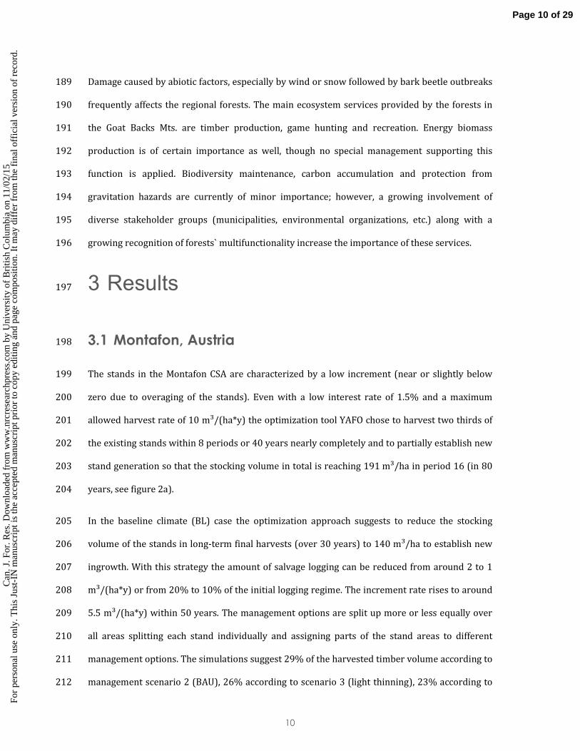
3 Results 197
3.1 Montafon, Austria 198
The stands in the Montafon CSA are characterized by a low increment (near or slightly below 199
zero due to overaging of the stands). Even with a low interest rate of 1.5% and a maximum 200
allowed harvest rate of 10 m³/(ha*y) the optimization tool YAFO chose to harvest two thirds of 201
the existing stands within 8 periods or 40 years nearly completely and to partially establish new 202
stand generation so that the stocking volume in total is reaching 191 m³/ha in period 16 (in 80 203
years, see figure 2a). 204
In the baseline climate (BL) case the optimization approach suggests to reduce the stocking 205
volume of the stands in long-term final harvests (over 30 years) to 140 m³/ha to establish new 206
ingrowth. With this strategy the amount of salvage logging can be reduced from around 2 to 1 207
m³/(ha*y) or from 20% to 10% of the initial logging regime. The increment rate rises to around 208
5.5 m³/(ha*y) within 50 years. The management options are split up more or less equally over 209
all areas splitting each stand individually and assigning parts of the stand areas to different 210
management options. The simulations suggest 29% of the harvested timber volume according to 211
management scenario 2 (BAU), 26% according to scenario 3 (light thinning), 23% according to 212
Page 10 of 29C
an. J
. For
. Res
. Dow
nloa
ded
from
ww
w.n
rcre
sear
chpr
ess.
com
by
Uni
vers
ity o
f B
ritis
h C
olum
bia
on 1
1/02
/15
For
pers
onal
use
onl
y. T
his
Just
-IN
man
uscr
ipt i
s th
e ac
cept
ed m
anus
crip
t pri
or to
cop
y ed
iting
and
pag
e co
mpo
sitio
n. I
t may
dif
fer
from
the
fina
l off
icia
l ver
sion
of
reco
rd.
11
scenario 4 (moderate thinning), and 22% according to scenario 1 (no management). The 213
ingrowth then is established according to stand type 2 (spruce-fir mix). 214
In the climate change scenario (A1B) the recommendations would change: The growing stock 215
would be reduced to even 96 m³/ha (within 35 years) to establish new ingrowth, finally 216
reaching 317 m³/ha in period 16 (in 80 years, see figure 2b), a much higher final standing 217
timber volume than without climatic change. With this strategy the present low increment rises 218
to slightly above 8 m³/(ha*y) within 55 years. The ratio of the BAU treatment increases initially 219
to 35%. 19% are treated according to scenario 3 (light thinning), 25% according to scenario 4 220
(moderate thinning) and 21% according to scenario 4 (no management). In the A1B case the 221
ingrowth should be established according to stand type 3 (spruce-fir-beech mix). The strategy 222
results in a two-phase shape of the harvest schedules. In phase 1 (reducing the stocking 223
volume), lasting for the first 35 years, in every period 10 m³/(ha*y) are harvested. Then 224
management switches to increase the growing stock. So in phase 2 the harvests are reduced to a 225
level of between 1 and 5 m³/(ha*y). 226
Additionally, our analysis shows the influence of a changing climate on tree species selection for 227
the ingrowth. In the BL scenario spruce-fir mixtures, defined as >95% of basal area comprised of 228
conifers, and beech-hardwood mixtures, defined as >25% of basal area comprised of beech are 229
dominating, whereas under scenario A1B the tree composition is switching to more spruce-fir-230
beech mixtures with a ratio of 5% - 25% in basal area made up of beech. 231
In a second optimization a minimum stock of 250 m³/ha was introduced as a constraint, 232
simulating a protection against avalanches and rockfall, soil erosion, local climate regulations, 233
water regulation or wildlife habitat that is provided by high stocking volumes. 234
In the BL case the initial growing stock will be reduced to around 280 m³/ha within 4 periods or 235
20 years to maintain the required 250 m³/ha after harvests (see figure 2c). After that initial 236
phase of volume reduction with harvests of 10 m³/(ha*y) a second phase starts with constant 237
growing stock levels and harvest rates between 3.5 and 6 m³/(ha*y). In the A1B case the 238
Page 11 of 29C
an. J
. For
. Res
. Dow
nloa
ded
from
ww
w.n
rcre
sear
chpr
ess.
com
by
Uni
vers
ity o
f B
ritis
h C
olum
bia
on 1
1/02
/15
For
pers
onal
use
onl
y. T
his
Just
-IN
man
uscr
ipt i
s th
e ac
cept
ed m
anus
crip
t pri
or to
cop
y ed
iting
and
pag
e co
mpo
sitio
n. I
t may
dif
fer
from
the
fina
l off
icia
l ver
sion
of
reco
rd.

12
schedule looks similar, but harvests are shifted more into the future (see figure 2d). The 239
ingrowth management differs as well. Whereas in the BL case the ingrowth is established 240
according to stand type 2 (spruce-fir mix) and 4 (beech-hardwood type), here stand type 3 241
(spruce-fir-beech mix) is chosen by the optimization approach. 242
In the BL case the provision of that minimum stock influences the risk in a desirable way as the 243
standard deviation of the NPV is decreasing from 74% to 50%. In the A1B case the risk 244
(standard deviation) is rising clearly from 59% to 124%. Accordingly, as we assume the 245
conditions of the BL case the provision of the minimum stock reduces the returns from -15 to -246
21 EUR/(ha*a) but does also slightly reduce financial risk. In the A1B case both variables are 247
influenced negatively by providing the ES service and we calculate lower returns with higher 248
risks. 249
The comparison of the annuities shows that the provision of the exemplary ES “protection 250
against avalanches and rockfall” costs 6 EUR/(ha*a) in the case of the BL scenario and 14 251
EUR/(ha*a) in the case of the climate change scenario. 252
Table 1 gives an overview of the financial results over the four optimization runs. In the A1B 253
case positive but small returns can be achieved whereas in the BL scenario the annuities are 254
negative. The reasons being generally low timber prices combined with high harvesting costs 255
due to the topographic conditions. As returns are near zero, the fluctuations caused by natural 256
disturbances and timber price changes lead to noticeably high relative standard deviations 257
(between 50% and 124%). The better growth of the ingrowth in the A1B case helps to raise the 258
returns to positive results. 259
260
Page 12 of 29C
an. J
. For
. Res
. Dow
nloa
ded
from
ww
w.n
rcre
sear
chpr
ess.
com
by
Uni
vers
ity o
f B
ritis
h C
olum
bia
on 1
1/02
/15
For
pers
onal
use
onl
y. T
his
Just
-IN
man
uscr
ipt i
s th
e ac
cept
ed m
anus
crip
t pri
or to
cop
y ed
iting
and
pag
e co
mpo
sitio
n. I
t may
dif
fer
from
the
fina
l off
icia
l ver
sion
of
reco
rd.

13
3.2 The Goat Backs Mts., Slovakia 261
As there are high salvage ratios in this case study region we also introduced a maximum harvest 262
volume of 10 m³/(ha*a) or 50 m³/(ha*period) to avoid a too intensive volume reduction of the 263
remaining stands within a couple of periods. 264
Figure 3a shows the biophysical results of the optimization for the BL case. The initial volume of 265
400 m³/ha (or 350 m³/ha after harvests) has been reduced to 152 m³/ha in periods 9 and 10 266
(i.e. within 45 to 50 years) and rises again to 246 m³/ha in period 18 (in 95 years). Over the 267
whole simulation period the restricted maximal harvest amounts of 10 m³/(ha*y) are used. By 268
reducing the stocking volumes new ingrowth is established reaching 212 m³/ha in period 18. 269
That means nearly all initial existing stands are harvested and transferred to a new stand 270
generation. The initial salvage logging volume of about 6.5 m³/(ha*y) is reduced to below 271
2.6 m³/(ha*y) in periods 5 to 18. After a phase where the management suggestion is focused on 272
final harvests (between periods 4 to 10) a second phase begins where mainly thinnings are 273
executed. This strategy helps to raise the increment from initially 4.5 m³/(ha*y) to a final level 274
between 12.0 and 13.0 m³/(ha*y). 275
Initially (in simulation period 0) 45% of the harvested timber is managed according to the 276
scenario “moderate thinning”. 28% is harvested according to “current management”, 22% 277
according to “no management” and 6% according to “light thinning”. But these ratios are highly 278
dependent on the investigated period. There is a tendency that in most cases “moderate 279
thinning” and “current management” are the preferred options. Within the simulated ingrowth 280
stands the stand type 3 (50% spruce, 30% pine, 20% beech) is clearly preferred. 281
As the differences between the BL and A1B climate scenario are small we show them in a 282
different representation. As such, figure 3c shows the differences of the harvest volume between 283
the baseline and the climate change scenario in each period. The harvested amounts are 284
additionally split by the four different management scenarios. There is a clear tendency for 285
Page 13 of 29C
an. J
. For
. Res
. Dow
nloa
ded
from
ww
w.n
rcre
sear
chpr
ess.
com
by
Uni
vers
ity o
f B
ritis
h C
olum
bia
on 1
1/02
/15
For
pers
onal
use
onl
y. T
his
Just
-IN
man
uscr
ipt i
s th
e ac
cept
ed m
anus
crip
t pri
or to
cop
y ed
iting
and
pag
e co
mpo
sitio
n. I
t may
dif
fer
from
the
fina
l off
icia
l ver
sion
of
reco
rd.

14
increasing differences between the two climate scenarios in the second part of the investigated 286
time horizon, with more harvests under climate change conditions. Also, in the second half of the 287
analyzed time horizon, the variant “no management” becomes less important whereas 288
increasing amounts of timber are harvested according to the close-to-nature management 289
scenario “moderate thinning” as well as the “current management” scenario. In the long term 290
(i.e. ingrowth management) stand type 3 dominates as it does in the BL case. 291
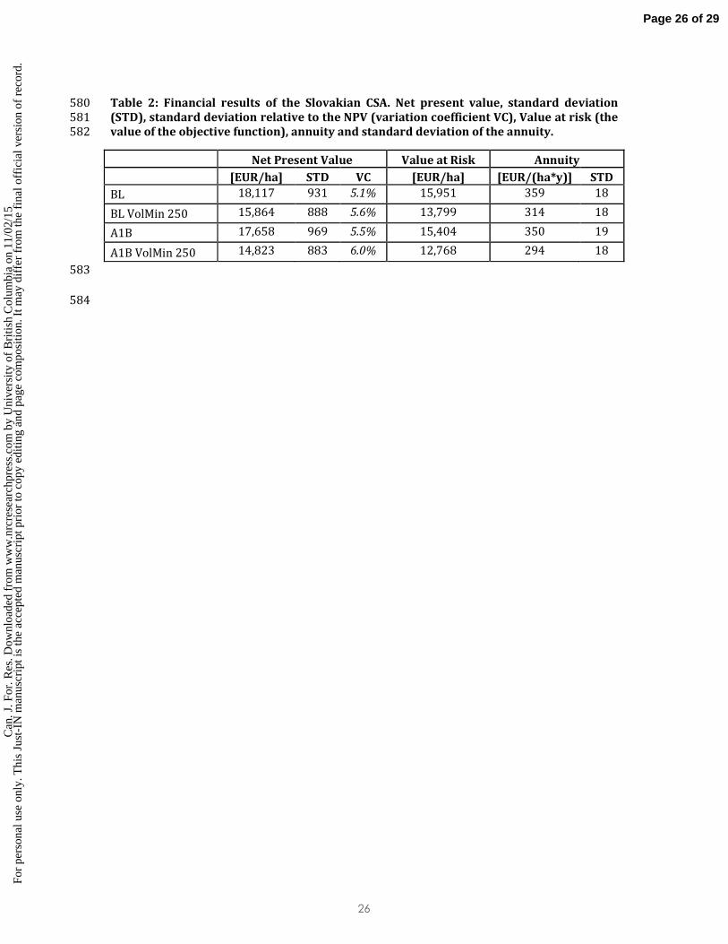
Table 2 gives an overview of the financial results. Comparing the lines “BL” and “A1B”, the 292
average annuity is reduced just slightly from 359 to 350 EUR/(ha*y). In both cases the standard 293
deviation is at 18 to 19 EUR/(ha*y) or 5.1 to 5.5%. This is an effect of the natural growth that is 294
only slightly reduced under climate change conditions. 295
In the second optimization design with a minimum stocking volume, the “u shape pattern” of the 296
volume development is graduated by this restriction leading to a temporarily reduction of the 297
harvest rate to 4.8 m³/(ha*y) in period 5 (in 25 years) that gradually rises again to 10.0 298
m³/(ha*y) in period 10 (in 50 years, see figure 3b for the BL case). 299
Figure 3d shows the same for the A1B case. The result is quite similar to the BL case. However, 300
due to the reduced growth under climate change conditions the reduction in harvests is more 301
severe. Also it is not possible to raise the volume considerably above the required 250 m³/ha at 302
the end of the investigated time horizon. The tree selection within the ingrowth is always 303
according to stand type 3 (50% spruce, 30% pine, 20% beech). 304
The comparison of the annuities shows that the provision of the ES costs 45 EUR/(ha*y) in the 305
case of the BL scenario and 56 EUR/(ha*y) in the case of the A1B scenario. That means, there is 306
only a slight difference between the scenarios. Under climate change conditions the costs rise 307
from 12% to 16% of the returns. In total, the costs for the provision of the ES are significant. 308
309
Page 14 of 29C
an. J
. For
. Res
. Dow
nloa
ded
from
ww
w.n
rcre
sear
chpr
ess.
com
by
Uni
vers
ity o
f B
ritis
h C
olum
bia
on 1
1/02
/15
For
pers
onal
use
onl
y. T
his
Just
-IN
man
uscr
ipt i
s th
e ac
cept
ed m
anus
crip
t pri
or to
cop
y ed
iting
and
pag
e co
mpo
sitio
n. I
t may
dif
fer
from
the
fina
l off
icia
l ver
sion
of
reco
rd.

15
4 Discussion & Conclusions 310
4.1 General 311
Our approach presents an optimization of harvest schedules under climate change and the 312
provisioning of an important ecosystem service (protection against avalanches and rockfall). 313
We choose two different case study areas for two reasons: First: one is in the Alpine region and 314
the other in low mountain range, so that we can cover most of the typical mountain forests in 315
Central Europe. Second: Our research explored the options for linking two forest dynamics 316
models (PICUS and SIBYLA) driven by an ensemble of climate change scenarios with a forest 317
management optimizer (YAFO) to analyze possible responses of management to climate change. 318
4.2 Climate change 319
Different to other approaches, such as Hanewinkel et al. (2010; 2013), the economic impact of 320
climatic change has been modelled more mechanistically in our study. While the mentioned 321
alternative studies use climate dependent presence/absence estimations for tree species to 322
predict the economic impact of climate change on forestry, the climate scenarios affect the 323
growth parameters and the survival curves directly. This leaves space for adapting the 324
management accordingly, which depends in first place on economic considerations (expected 325
return and risk). 326
4.3 Ecosystem services 327
While climatic change impacts on the growth rates and the survival probabilities, the ecosystem 328
service is addressed through a constraint (minimum stocking of 250 m³/ha). Advantages of this 329
approach are the optimization perspective, which suggests management strategies at a 330
minimum of opportunity costs. Also, the costs for providing the ecosystem service may be 331
derived, which is important for discussions with stakeholders. Another advantage is that the 332
constraint guarantees the required level, for example of the standing timber in our case. Thus, 333
Page 15 of 29C
an. J
. For
. Res
. Dow
nloa
ded
from
ww
w.n
rcre
sear
chpr
ess.
com
by
Uni
vers
ity o
f B
ritis
h C
olum
bia
on 1
1/02
/15
For
pers
onal
use
onl
y. T
his
Just
-IN
man
uscr
ipt i
s th
e ac
cept
ed m
anus
crip
t pri
or to
cop
y ed
iting
and
pag
e co
mpo
sitio
n. I
t may
dif
fer
from
the
fina
l off
icia
l ver
sion
of
reco
rd.

16
possibly very high levels of other services, such as timber production, cannot serve to 334
compensate for smaller than demanded protective services. 335
There are only few studies including ecosystem services into optimization on landscape of larger 336
scales. Nelson et al. (2009) and Goldstein et al. (2012) carried out scenario analyses at landscape 337
scale considering a limited number of pre-defined scenarios. In contrast, Wise et al. (2009) 338
imposed a carbon tax to take into account climate regulation services into land-use optimization. 339
This study used a highly complex world dynamic recursive model including energy, economy, 340
agriculture, land use, and land cover based on economic equilibrium in energy and agriculture 341
markets. Bateman et al. (2013) carried out land-use optimization for the UK under the impact of 342
climatic change and integration of ecosystem services. These were considered in the modelling 343
through hypothetical financial payments, for example, for recreation. In contrast to the study by 344
Bateman et al. (2013), our study has been more conservative, including the protective function 345
via a constraint and not via estimated willingness to pay for a service. Our higher 346
conservativeness might have the advantage of a higher reliability of the results obtained, 347
because estimates on the value of ecosystem services are known to be highly uncertain (see, for 348
example, ranges reported by Costanza et al. (1997). Also, none of the mentioned sophisticated 349
studies integrated uncertainty into their analyses. An example how to integrate carbon storage 350
as an ecosystem service in optimized tropical land-use allocation under the risk of fluctuating 351
product prices has been provided by Knoke et al. (2013). However, a focus on mountain forest 352
management combined with a sophisticated modelling of survival and price risks has been 353
lacking in the studies discussed. 354
Of course, there are many alternatives to integrate multiple ecosystem services into 355
optimization (see Uhde et al. 2015 for an overview). However, these options, for example Goal 356
Programming (Tamiz und Jones 1998), may become quite complex when considering multiple 357
forest stands under risk simultaneously. Still, there is ample opportunity to develop further the 358
optimized forest management under multiple objectives. An ultimate advantage of the 359
Page 16 of 29C
an. J
. For
. Res
. Dow
nloa
ded
from
ww
w.n
rcre
sear
chpr
ess.
com
by
Uni
vers
ity o
f B
ritis
h C
olum
bia
on 1
1/02
/15
For
pers
onal
use
onl
y. T
his
Just
-IN
man
uscr
ipt i
s th
e ac
cept
ed m
anus
crip
t pri
or to
cop
y ed
iting
and
pag
e co
mpo
sitio
n. I
t may
dif
fer
from
the
fina
l off
icia
l ver
sion
of
reco
rd.
17
quantitative programming approaches over the so far often scenario based approaches to 360
include ecosystem services is certainly that strategies result from well-defined objective 361
functions and constraints. The resulting scenarios may, hence, be defended well in public 362
discussions. Also, it is possible to revise optimizations, when stakeholders mention new 363
expectations. 364
4.4 Austrian case study area 365
The Austrian CSA showed a positive influence of the climate change scenario on the results – in 366
the sense of a better economic result. A possible explanation is the fact that the growth of the 367
trees increases under climate change scenario A1B leading to positive annuities compared to the 368
BL climate scenario. 369
In both cases the recommendations that arise for the practitioner are to reduce the growing 370
stock of the currently overaged stands to establish new ingrowth leading to an overall reduction 371
of age and related risk as well as an increase in growth. This reduction should be done slowly 372
over a planning period of 35 to 50 years to further reduce financial and biophysical risks that 373
increase with increasing aerial size of harvesting activities. 374
If a minimum growing stock of 250 m³/ha is to be maintained, volume reduction has to be 375
stopped after 20 years to allow the introduction of a management regime focusing on constant 376
levels of growing stock on the enterprise level. To allow for such a beneficial development, 377
around 40% of the total area (64 ha) have to be managed for the establishment of regeneration 378
raising the increment rate so that within 60 years an annual increment and harvest rates of 379
about 5 m³/(ha*y) become possible. 380
Our results for the A1B scenario show an increase share of hardwood within the chosen 381
management options for the ingrowth. That means, under climate change conditions the 382
admixing of hardwoods to softwood stands should be emphasized to count for the changing 383
growth conditions in the Austrian CSA. Although that effect is primarily based on simulated 384
Page 17 of 29C
an. J
. For
. Res
. Dow
nloa
ded
from
ww
w.n
rcre
sear
chpr
ess.
com
by
Uni
vers
ity o
f B
ritis
h C
olum
bia
on 1
1/02
/15
For
pers
onal
use
onl
y. T
his
Just
-IN
man
uscr
ipt i
s th
e ac
cept
ed m
anus
crip
t pri
or to
cop
y ed
iting
and
pag
e co
mpo
sitio
n. I
t may
dif
fer
from
the
fina
l off
icia
l ver
sion
of
reco
rd.

18
changes in growth, this result is comparable with the 20% beech admixture necessary for the 385
reduction of financial risks found by Roessiger et al. (2011) as well as a 7% admixture of beech 386
into spruce stands described by Griess et al. (2012), to achieve a distinctive reduction of risk. 387
4.5 Slovakian case study area 388
In the Slovakian CSA the results show similar main patterns as those for the Austrian CSA. The 389
recommendation is to initially reduce growing stock to around 150-200 m³/ha to improve 390
increment rates and to reduce risk, i.e. the ratio of salvage logging, leading to annuities of 280 to 391
320 EUR/(ha*y). On the contrary to the Austrian CSA, the harvest rates can be held constant 392
over the entire planning horizon as increment rates are much higher. For the management of 393
ingrowth a tree mixture of 50% spruce, 30% pine and 20% beech is preferred over the other 394
options (see online supplement). To compensate for the reduced growth, in the A1B climate 395
scenario this should be accompanied by managing more and more stands according to “current 396
management” or “moderate thinning” reducing the area without any management. 397
If a volume minimum growing stock of 250 m³/ha is to be maintained, harvests have to be 398
reduced to around 6 m³/(ha*y) during the first 25 years. After that they can be gradually be 399
increased back to the initial 10 m³/(ha*y) over a time span of 30 years as the increment rate 400
increases over time. 401
The most interesting result for Slovakia is the increasing relevance of the “moderate thinning” 402
and “current management” scenarios under a changing climate. One explanation is that due to 403
the slightly reduced growth in that case the additional increment of the remaining trees induced 404
by slightly more intensified thinning can compensate losses in growth better than any other 405
management option. 406
4.6 General conclusions 407
The comparison of both CSAs shows that it is in fact possible to derive some general 408
recommendations for optimum forest management strategies under a changing climate. We can 409
Page 18 of 29C
an. J
. For
. Res
. Dow
nloa
ded
from
ww
w.n
rcre
sear
chpr
ess.
com
by
Uni
vers
ity o
f B
ritis
h C
olum
bia
on 1
1/02
/15
For
pers
onal
use
onl
y. T
his
Just
-IN
man
uscr
ipt i
s th
e ac
cept
ed m
anus
crip
t pri
or to
cop
y ed
iting
and
pag
e co
mpo
sitio
n. I
t may
dif
fer
from
the
fina
l off
icia
l ver
sion
of
reco
rd.

19
recommend the reduction of growing stock levels to improve ingrowth rates and shifting the 410
tree selection within the ingrowth towards hardwood ratios of up to 20%. Our results 411
correspond with the findings of Griess & Knoke (2013) or Brang et al. (2014) who derived 6 412
principles for enhancing the adaptability of forests within close-to-nature silviculture. Our 413
results confirm the principles of increasing tree species richness, increasing structural diversity, 414
replacing high-risk stands and reducing average growing stocks for a successful sustainable 415
forest management in the long term. 416
However, some problems remain unresolved, and are subject to further research: The fact that 417
the forest dynamics models (PICUS and SIBYLA) are not interactively connected with the 418
optimizer (YAFO) required to deliver model output in form of an ingrowth table (specific to each 419
climate change scenario and providing data for different ingrowth options). This output table 420
governed the growth process in the optimizer after thinning or harvesting operations. So, the 421
differences in growth process governed by an ingrowth table and by the forest dynamics model 422
should be kept in mind. If a direct bi-directional interface between the two parts that our 423
methodology requires (simulation + optimization) would be made available it would be possible 424
to integrate changes in growth due to thinning or harvesting directly. 425
Furthermore, the decision the optimizer suggests regarding ingrowth is highly dependent on the 426
simulated time horizon. If another tree mixture would be superior in the long run the model 427
cannot include this in its decision. So the proposed management strategy has always to be seen 428
as the best decision based on what we know today. If knowledge changes the planning has to be 429
updated. A limitation that applies to all scientific outputs. To make inclusion of such changes into 430
future research easier it would be desirable to develop the interface mentioned earlier as well as 431
to further develop growth & yield models to allow the production of stand information in a fast 432
and reliable way. This could be done by further developing the necessary model parts with a 433
focus on user friendliness, adaptability as well as computing capacity to reduce model runtimes. 434
Page 19 of 29C
an. J
. For
. Res
. Dow
nloa
ded
from
ww
w.n
rcre
sear
chpr
ess.
com
by
Uni
vers
ity o
f B
ritis
h C
olum
bia
on 1
1/02
/15
For
pers
onal
use
onl
y. T
his
Just
-IN
man
uscr
ipt i
s th
e ac
cept
ed m
anus
crip
t pri
or to
cop
y ed
iting
and
pag
e co
mpo
sitio
n. I
t may
dif
fer
from
the
fina
l off
icia
l ver
sion
of
reco
rd.

20
Finally, the simplification of the effect of a changing climate on forest development has to be 435
kept in mind when converting our findings into practical recommendations. While a 436
comprehensive and detailed evaluation of the tree growth subject to climate change showed 437
differential responses along the elevation gradient (e.g. Hlásny et al. submitted), the outputs of 438
the optimization presented here were produced assuming an average response for the entire 439
CSA based on a single ingrowth table. Therefore, further modifications of the methodology 440
would be needed to allow using outputs as a direct guide for forest management planning. A 441
possible solution could be to run the optimization separately for several elevation zones which 442
show differential growth response to climate change. 443
Even though the limitations named above are important and will need further work to be fully 444
overcome, our research presents first findings of its kind, combining information from different 445
areas and forest dynamics models to derive optimized management plans for larger areas. Our 446
work allows a comparison of the differences in forest development over a large European 447
mountain area and can be seen as a first step towards a wider analysis of what climate change 448
will mean for our European forests, what we can do to adapt our management towards 449
upcoming changes as well as towards finding ways to allow consideration of ecosystem services 450
in optimized forest management planning on larger scales. Additionally, our research can be 451
seen as a guideline regarding what information is necessary, to develop improved forest 452
management models, an area of outstanding future importance. As the significant societal 453
changes over the last decades and the emergence of new policies, (e.g. on biodiversity, bioenergy 454
and climate change clearly) present the need to enhance sustainability of multipurpose forestry 455
in the European Union. 456
457
Page 20 of 29C
an. J
. For
. Res
. Dow
nloa
ded
from
ww
w.n
rcre
sear
chpr
ess.
com
by
Uni
vers
ity o
f B
ritis
h C
olum
bia
on 1
1/02
/15
For
pers
onal
use
onl
y. T
his
Just
-IN
man
uscr
ipt i
s th
e ac
cept
ed m
anus
crip
t pri
or to
cop
y ed
iting
and
pag
e co
mpo
sitio
n. I
t may
dif
fer
from
the
fina
l off
icia
l ver
sion
of
reco
rd.

21
5 Acknowledgements 458
The study presented here is part of the project “ARANGE - Advanced multifunctional forest 459
management in European mountain ranges” (FP7-KBBE-2011-5) is funded by the European 460
Commission, Seventh Framework Program under grant agreement number 289437. The authors 461
wish to thank John Jacobs for the language editing of the manuscript. 462
463
6 References 464
Anderegg, W. R. L.; Kane, J. M.; Anderegg, L. D. L. (2012): Consequences of widespread tree 465
mortality triggered by drought and temperature stress. Nature Climate Change 3 (1), 30–36. 466
Bateman, I. J.; Harwood, A. R.; Mace, G. M.; Watson, R. T.; Abson, D. J.; Andrews, B. et al. (2013): 467
Bringing Ecosystem Services into Economic Decision-Making: Land Use in the United Kingdom. 468
In: Science 341 (6141), 45–50. 469
Bjørnstad, E.; Skonhoft, A. (2002): Wood Fuel or Carbon Sink? Aspects of Forestry in the Climate 470
Question. Environmental and Resource Economics 23 (4), 447-465. 471
Brang, P.; Spathelf, P.; Larsen, J. B.; Bauhus, J.; Boncina, A.; Chauvin, C. et al. (2014): Suitability of 472
close-to-nature silviculture for adapting temperate European forests to climate change. Forestry 473
87 (4), 492–503. 474
Bußjäger, P. (2007): zu Luxusbauten wird kein Holz verabfolgt! - Die Geschichte des Forstfonds 475
des Standes Montafon. In: Malin, H.; Maier, B.; Dönz-Breuß. M. (eds.): Montafoner Standeswald - 476
Montafoner Schriftenr. 18. Heimatschutzverein Montafon, Schruns, 9–24. 477
Cordonnier, T.; Berger, F.; Elkin, C.; Lämas, T.; Martinez, M. (2013): Models and linker functions 478
(indicators) for ecosystem services. Arange Deliverable D2.2, Project Report, FP7-289437-479
ARANGE, 94 pp. 480
Costanza, R.; D'Arge, R.; Groot, R. de; Farber, S.; Grasso, M.; Hannon, B. et al. (1997): The value of 481
the world's ecosystem services and natural capital. In: Nature 387 (6630), 253–260. 482
EEA (2010): Europe's ecological backbone: recognising the true value of our mountains. 483
European Environment Agency. Copenhagen. 484
Page 21 of 29C
an. J
. For
. Res
. Dow
nloa
ded
from
ww
w.n
rcre
sear
chpr
ess.
com
by
Uni
vers
ity o
f B
ritis
h C
olum
bia
on 1
1/02
/15
For
pers
onal
use
onl
y. T
his
Just
-IN
man
uscr
ipt i
s th
e ac
cept
ed m
anus
crip
t pri
or to
cop
y ed
iting
and
pag
e co
mpo
sitio
n. I
t may
dif
fer
from
the
fina
l off
icia
l ver
sion
of
reco
rd.
22
Frehner, M.; Wasser, B.; Schwitter, R. (2005): Nachhaltigkeit und Erfolgskontrolle im 485
Schutzwald. Wegleitung für Pflegemassnahmen in Wäldern mit Schutzfunktion. Bundesamt für 486
Umwelt. Bern. 487
Goldstein, J. H.; Caldarone, G.; Duarte, T. K.; Ennaanay, D.; Hannahs, N.; Mendoza, G. et al. (2012): 488
Integrating ecosystem-service tradeoffs into land-use decisions. In: Proceedings of the National 489
Academy of Sciences 109 (19), 7565–7570. 490
Griess, V.C.; Knoke, T. (2013): Bioeconomic modeling of mixed Norway spruce—European beech 491
stands: economic consequences of considering ecological effects. Eur J Forest Res 132 (3), 511-492
522. 493
Griess, V.C.; Acevedo, R.; Härtl, F.; Staupendahl, K.; Knoke, T. (2012): Does mixing tree species 494
enhance stand resistance against natural hazards? A case study for spruce. Forest Ecology and 495
Management. 267: 284-296. 496
Grunewald, K.; Bastian, O. (2015): Ecosystem assessment and management as key tools for 497
sustainable landscape development: A case study of the Ore Mountains region in Central Europe. 498
Ecological Modelling 295, 151–162. 499
Hanewinkel, M.; Cullmann, D. A.; Schelhaas, M.-J; Nabuurs, G.-J; Zimmermann, N. E. (2013): 500
Climate change may cause severe loss in the economic value of European forest land. In: Nature 501
Clim. Change 3 (3), 203–207. 502
Hanewinkel, M.; Hummel, S.; Cullmann, D. A. (2010): Modelling and economic evaluation of 503
forest biome shifts under climate change in Southwest Germany. In: Forest Ecology and 504
Management 259 (4), 710–719. 505
Härtl, F. (2015): Der Einfluss des Holzpreises auf die Konkurrenz zwischen stofflicher und 506
thermischer Holzverwertung. Ein forstbetrieblicher Planungsansatz unter Berücksichtigung von 507
Risikoaspekten. Dissertation. Technische Universität München, Freising-Weihenstephan. 508
Fachgebiet für Waldinventur und nachhaltige Nutzung. 509
Härtl, F.; Hahn, A.; Knoke, T. (2013): Risk-sensitive planning support for forest enterprises: The 510
YAFO model. Computers and Electronics in Agriculture (94), 58–70. 511
Hlásny, T.; Barka, I.; Kulla, L.; Bucha, T.; Sedmák, R:; Trombik, J.: Sustainability of forest 512
ecosystem services provisioning in Central European mountain forests: The role of climate 513
change. Submitted to Regional Environmental Change. 514
Knoke, T.; Calvas, B.; Moreno, S. O.; Onyekwelu, J. C.; Griess, V. C. (2013): Food production and 515
climate protection—What abandoned lands can do to preserve natural forests. In: Global 516
Environmental Change 23 (5), 1064–1072. 517
Knoke, T.; Stimm, B.; Weber, M. (2008): Tropical farmers need productive alternatives. Nature 518
452 (7190), 934. 519
Page 22 of 29C
an. J
. For
. Res
. Dow
nloa
ded
from
ww
w.n
rcre
sear
chpr
ess.
com
by
Uni
vers
ity o
f B
ritis
h C
olum
bia
on 1
1/02
/15
For
pers
onal
use
onl
y. T
his
Just
-IN
man
uscr
ipt i
s th
e ac
cept
ed m
anus
crip
t pri
or to
cop
y ed
iting
and
pag
e co
mpo
sitio
n. I
t may
dif
fer
from
the
fina
l off
icia
l ver
sion
of
reco
rd.

23
Knoke, T.; Wurm, J. (2006): Mixed forests and a flexible harvest policy: a problem for 520
conventional risk analysis? European Journal of Forest Research 125 (3), 303–315. 521
Kolström, M.; Lindner, M.; Vilén, T.; Maroschek, M.; Seidl, R.; Lexer, M. J. et al. (2011): Reviewing 522
the Science and Implementation of Climate Change Adaptation Measures in European Forestry. 523
Forests 2 (4), 961–982. 524
Lindner, M.; Maroschek, M.; Netherer, S.; Kremer, A.; Barbati, A.; Garcia-Gonzalo, J. et al. (2010): 525
Climate change impacts, adaptive capacity, and vulnerability of European forest ecosystems. 526
Adaptation of Forests and Forest Management to Changing Climate. Selected papers from the 527
conference on “Adaptation of Forests and Forest Management to Changing Climate with 528
Emphasis on Forest Health: A Review of Science, Policies and Practices”, Umeå, Sweden, August 529
25-28, 2008 259 (4), 698–709. 530
Malin, H.; Maier, B. (2007): Der Wald - Das grüne Rückgrat des Montafon. In: Malin, H.; Maier, B.; 531
Dönz-Breuß, M. (eds): Montafoner Standeswald - Montafoner Schriftenreihe 18. 532
Heimatschutzverein Montafon, Schruns, 91–114. 533
Malin, H.; Lerch, T. (2007): Schutzwaldbewirtschaftung im Montafon. In: Malin, H.; Maier, B.; 534
Dönz-Breuß, M. (eds): Montafoner Standeswald - Montafoner Schriftenreihe 18. 535
Heimatschutzverein Montafon, Schruns, 115–128. 536
Markowitz, H. M. (1952): Portfolio Selection. The Journal of Finance (7), 77–91. 537
Markowitz, H. M. (2010): Portfolio Theory: As I Still See It. Annual Review of Financial 538
Economics 2 (1), 1-23. 539
Maroschek, M.; Seidl, R.; Netherer, S.; Lexer, M. J. (2009): Climate change impacts on goods and 540
services of European mountain forests. Unasylva 60 (231/232), 76–80. 541
Möhring, B.; Rüping, U. (2008): A concept for the calculation of financial losses when changing 542
the forest management strategy. Forest Policy and Economics 10 (3), 98–107. 543
Nelson, E.; Mendoza, G.; Regetz, J.; Polasky, S.; Tallis, H.; Cameron, D. R. et al. (2009): Modeling 544
multiple ecosystem services, biodiversity conservation, commodity production, and tradeoffs at 545
landscape scales. In: Frontiers in Ecology and the Environment 7 (1), 4–11. 546
Niinimäki, S.; Tahvonen, O.; Mäkelä, A.; Linkosalo, T. (2013): On the economics of Norway spruce 547
stands and carbon storage. Canadian Journal of Forest Research 43 (7), 637–648. 548
O'Hara, K. L.; Ramage, B. S. (2013): Silviculture in an uncertain world: utilizing multi-aged 549
management systems to integrate disturbance. Forestry 86 (4), 401–410. 550
Pihlainen, S.; Tahvonen, O.; Niinimäki, S. (2014): The economics of timber and bioenergy 551
production and carbon storage in Scots pine stands. Canadian Journal of Forest Research 44 (9), 552
1091–1102. 553
Page 23 of 29C
an. J
. For
. Res
. Dow
nloa
ded
from
ww
w.n
rcre
sear
chpr
ess.
com
by
Uni
vers
ity o
f B
ritis
h C
olum
bia
on 1
1/02
/15
For
pers
onal
use
onl
y. T
his
Just
-IN
man
uscr
ipt i
s th
e ac
cept
ed m
anus
crip
t pri
or to
cop
y ed
iting
and
pag
e co
mpo
sitio
n. I
t may
dif
fer
from
the
fina
l off
icia
l ver
sion
of
reco
rd.

24
Reid, W. V.; Mooney, H. A.; Capistrano, D.; Carpenter, S. R.; Chopra, K.; Cropper, A. et al. (2006): 554
Nature: the many benefits of ecosystem services. Nature 443 (7113), 749. 555
Rist, L.; Felton, A.; Samuelsson, L.; Sandström, C.; Rosvall, O. (2013): A New Paradigm for 556
Adaptive Management. Ecology and Society 18 (4). 557
Roessiger, J.; Griess, V. C.; Knoke, T. (2011): May risk aversion lead to near-natural forestry? A 558
simulation study. Forestry 84 (5), 527–537. 559
Schober, R. (1987): Ertragstafeln wichtiger Baumarten bei verschiedener Durchforstung. 3. Aufl. 560
Frankfurt am Main: Sauerländer. 561
Seidl, R.; Rammer, W.; Lexer, M. J. (2011): Climate change vulnerability of sustainable forest 562
management in the Eastern Alps. Climatic Change 106 (2), 225–254. 563
Tamiz, M.; Jones, D. Romero C. (1998): Goal programming for decision making: An overview of 564
the current state-of-the-art. In: European Journal of Operational Research 111 (3), 569–581. 565
Uhde, B.; Hahn, W. A.; Griess, V. C.; Knoke, T. (2015): Hybrid MCDA Methods to Integrate Multiple 566
Ecosystem Services in Forest Management Planning: A Critical Review. In: Environmental 567
Management, 1-16. 568
Waller, L. A.; Smith, D.; Childs, J. E.; Real, L. A. (2003): Monte Carlo assessments of goodness-of-fit 569
for ecological simulation models. Ecological Modelling 164 (1), 49–63. 570
Wise, M.; Calvin, K.; Thomson, A.; Clarke, L.; Bond-Lamberty, B.; Sands, R. et al. (2009): 571
Implications of Limiting CO2 Concentrations for Land Use and Energy. In: Science 324 (5931), 572
1183–1186. 573
574
Page 24 of 29C
an. J
. For
. Res
. Dow
nloa
ded
from
ww
w.n
rcre
sear
chpr
ess.
com
by
Uni
vers
ity o
f B
ritis
h C
olum
bia
on 1
1/02
/15
For
pers
onal
use
onl
y. T
his
Just
-IN
man
uscr
ipt i
s th
e ac
cept
ed m
anus
crip
t pri
or to
cop
y ed
iting
and
pag
e co
mpo
sitio
n. I
t may
dif
fer
from
the
fina
l off
icia
l ver
sion
of
reco
rd.

25
Table 1: Financial results of the Montafon CSA. Net present value, standard deviation 575 (STD), standard deviation relative to the NPV (variation coefficient VC), Value at risk (the 576 value of the objective function), annuity and standard deviation of the annuity. 577
Net Present Value Value at Risk Annuity
[EUR/ha] STD VC [EUR/ha] [EUR/(ha*a)] STD
BL -731 540 74% -1,986 -15 11
BL VolMin 250 -1,008 504 50% -2,180 -21 11
A1B 1,127 661 59% -411 24 14
A1B VolMin 250 467 580 124% -881 10 12
578
579
Page 25 of 29C
an. J
. For
. Res
. Dow
nloa
ded
from
ww
w.n
rcre
sear
chpr
ess.
com
by
Uni
vers
ity o
f B
ritis
h C
olum
bia
on 1
1/02
/15
For
pers
onal
use
onl
y. T
his
Just
-IN
man
uscr
ipt i
s th
e ac
cept
ed m
anus
crip
t pri
or to
cop
y ed
iting
and
pag
e co
mpo
sitio
n. I
t may
dif
fer
from
the
fina
l off
icia
l ver
sion
of
reco
rd.
26
Table 2: Financial results of the Slovakian CSA. Net present value, standard deviation 580 (STD), standard deviation relative to the NPV (variation coefficient VC), Value at risk (the 581 value of the objective function), annuity and standard deviation of the annuity. 582
Net Present Value Value at Risk Annuity [EUR/ha] STD VC [EUR/ha] [EUR/(ha*y)] STD
BL 18,117 931 5.1% 15,951 359 18
BL VolMin 250 15,864 888 5.6% 13,799 314 18
A1B 17,658 969 5.5% 15,404 350 19
A1B VolMin 250 14,823 883 6.0% 12,768 294 18
583
584
Page 26 of 29C
an. J
. For
. Res
. Dow
nloa
ded
from
ww
w.n
rcre
sear
chpr
ess.
com
by
Uni
vers
ity o
f B
ritis
h C
olum
bia
on 1
1/02
/15
For
pers
onal
use
onl
y. T
his
Just
-IN
man
uscr
ipt i
s th
e ac
cept
ed m
anus
crip
t pri
or to
cop
y ed
iting
and
pag
e co
mpo
sitio
n. I
t may
dif
fer
from
the
fina
l off
icia
l ver
sion
of
reco
rd.

27
Simulation of growth & yield data,
Using PICUS for the Austrian CSA and SIBYLA for Slovakia.
585
Figure 1: Data flow and description of the overall modelling + optimization approach 586
587
Page 27 of 29C
an. J
. For
. Res
. Dow
nloa
ded
from
ww
w.n
rcre
sear
chpr
ess.
com
by
Uni
vers
ity o
f B
ritis
h C
olum
bia
on 1
1/02
/15
For
pers
onal
use
onl
y. T
his
Just
-IN
man
uscr
ipt i
s th
e ac
cept
ed m
anus
crip
t pri
or to
cop
y ed
iting
and
pag
e co
mpo
sitio
n. I
t may
dif
fer
from
the
fina
l off
icia
l ver
sion
of
reco
rd.

28
588
Figure 2: Development of the growing stock (VolRem) and the timber amounts harvested 589 (VolHarvest). Results from the Austrian CSA. a: BL scenario. b: A1B scenario. c: BL 590 scenario, where additionally a minimum stocking volume of 250 m³/ha is required. d: 591 A1B scenario with the same minimum stocking volume required 592
593
594
595
596
597
598
Page 28 of 29C
an. J
. For
. Res
. Dow
nloa
ded
from
ww
w.n
rcre
sear
chpr
ess.
com
by
Uni
vers
ity o
f B
ritis
h C
olum
bia
on 1
1/02
/15
For
pers
onal
use
onl
y. T
his
Just
-IN
man
uscr
ipt i
s th
e ac
cept
ed m
anus
crip
t pri
or to
cop
y ed
iting
and
pag
e co
mpo
sitio
n. I
t may
dif
fer
from
the
fina
l off
icia
l ver
sion
of
reco
rd.

29
599
Figure 3: Development of the growing stock (VolRem) and the amounts harvested 600 (VolHarvest). Results from the Slovakian CSA. a: BL scenario. b: BL scenario, where 601 additionally a minimum stocking volume of 250 m³/ha is required. c: Difference of the 602 amounts harvested between the climate change scenario and the baseline scenario: a 603 positive value means more harvests under climate change conditions. “CuMngmt”: 604 current management (BAU). ”NoMngmt”: no management. “LightThin”: light thinning. 605 “ModThin”: a moderate close-to-nature thinning. d: A1B scenario, where additionally a 606 minimum stocking volume of 250 m³/ha is required 607
608
Page 29 of 29C
an. J
. For
. Res
. Dow
nloa
ded
from
ww
w.n
rcre
sear
chpr
ess.
com
by
Uni
vers
ity o
f B
ritis
h C
olum
bia
on 1
1/02
/15
For
pers
onal
use
onl
y. T
his
Just
-IN
man
uscr
ipt i
s th
e ac
cept
ed m
anus
crip
t pri
or to
cop
y ed
iting
and
pag
e co
mpo
sitio
n. I
t may
dif
fer
from
the
fina
l off
icia
l ver
sion
of
reco
rd.
Top Related