

![Ranking Decision making units using Fuzzy Multi-Objective ......Multi-objective Linear Programming (MOLP) Veeramani et al. [23] Multi-objective Linear Programming (MOLP) Problems is](https://static.fdocuments.us/doc/165x107/610e91b630eca77d674f86aa/ranking-decision-making-units-using-fuzzy-multi-objective-multi-objective.jpg)


Languages
Pages
Legal


Multi-Objective Multi-Project Construction
Scheduling Optimization
Mohammed Saeed Khalil El-Abbasy
A Thesis
In the Department
of
Building, Civil, and Environmental Engineering
Presented in Partial Fulfillment of the Requirements
For the Degree of
Doctor of Philosophy (Building Engineering) at
Concordia University
Montreal, Quebec, Canada
February 2015
© Mohammed Saeed Khalil El-Abbasy, 2015

CONCORDIA UNIVERSITY
SCHOOL OF GRADUATE STUDIES
This is to certify that the thesis prepared
By: Mohammed Saeed El-Abbasy
Entitled: Multi-Objective Multi-Project Construction Scheduling Optimization
and submitted in partial fulfillment of the requirements for the degree of
DOCTOR OF PHILOSOPHY (Building Engineering)
complies with the regulations of the University and meets the accepted standards with respect
to originality and quality.
Signed by the final examining committee:
Chair
Dr. N. Bhuiyan
External Examiner
Dr. K. El-Rayes
External to Program
Dr. G. Gopakumar
Examiner
Dr. Z. Zhu
Examiner
Dr. O. Moselhi
Thesis Co-Supervisor
Dr. T. Zayed
Thesis Co-Supervisor
Dr. A. Elazouni
Approved By:
Dr. F. Haghighat, Graduate Program Director
February 11, 2015
Dr. A. Asif, Interim Dean
Faculty of Engineering & Computer Science

iii
ABSTRACT
Multi-Objective Multi-Project Construction Scheduling Optimization
Mohammed Saeed Khalil El-Abbasy, Ph.D.
Concordia University, 2015
In construction industry, contractors usually manage and execute multiple projects
simultaneously within their portfolio. This involves sharing of limited resources such as
funds, equipment, manpower, and others among different projects, which increases the
complexity of the scheduling process. The allocation of scarce resources then becomes a
major objective of the problem and several compromises should be made to solve the
problem to the desired level of optimality. In such cases, contractors are generally
concerned with optimizing a number of different objectives, often conflicting among each
other. Thus, the main objective of this research is to develop a multi-objective scheduling
optimization model for multiple construction projects considering both financial and
resource aspects under a single platform. The model aims to help contractors in devising
schedules that obtain optimal/near optimal tradeoffs between different projects’
objectives, namely: duration of multiple projects, total cost, financing cost, maximum
required credit, profit, and resource fluctuations. Moreover, the model offers the
flexibility in selecting the desired set of objectives to be optimized together. Three
management models are built in order to achieve the main objective which involves the
development of: (1) a scheduling model that establishes optimal/near optimal schedules
for construction projects; (2) a resource model to calculate the resource fluctuations and
iv
maximum daily resource demand; and (3) a cash flow model to calculate projects’
financial parameters. The three management models are linked with the designed
optimization model, which consequently performs operations of the elitist non-dominated
sorting genetic algorithm (NSGA-II) technique, in three main phases: (1) population
initialization; (2) fitness evaluation; and (3) generation evolution. The optimization
model is implemented and tested using different case studies of different project sizes
obtained from literature. Finally, an automated tool using C# language is built with a
friendly graphical user interface to facilitate solving multi-objective scheduling
optimization problems for contractors and practitioners.

v
إهداء إىلوالدتي الغالية "صفاء العباسي" ووالدي الغايل "سعيد العباسي"
توأم روحي زوجتي احلبيبة الغالية "داليا نوح"
قرة عيني ابنتي احلبيبة الغالية "أمرية"
اخوتي واخواتي األعزاء
Dedicated To
My beloved mother “Safaa El-Abbasy” and inspiring father “Saeed El-Abbasy”
My soulmate, beautiful, and supportive wife “Dalia Nouh”
My little lovely daughter and precious angel “Amira”
My dear brother and sisters and their kids

vi
ACKNOWLEDGEMENT
All gratitude and praise are due to ALLAH almighty who aided and guided me to bring
this thesis to light.
No words could ever express my deepest love and gratitude to my mother “Safaa El-
Abbasy” and father “Saeed El-Abbasy” for sacrificing a lot to make me, my brother and
sisters what we are today, something we have often missed to acknowledge. They have
been and will always be my idols and their enthusiasm to see the completion of this work
was above all a significant motivator.
Most of all, my greatest indebtedness and deepest appreciation is to my lovely wife and
soulmate “Dalia Nouh”. Nothing is compared to her warm-heartedness and care, and
her unconditional and continuous support to accomplish this thesis. Her contribution to
this work is endless. She simply made it all possible.
My daughter and little princess “Amira”, one day when you grow up and read these
lines, you will know how much you contributed to this work by just a simple smile from
you, by just a simple hug from you, and mostly by just being you. I owe you a lot for all
the time I took away from you to accomplish this work.
Much gratitude is also due to my brother “Khaled” and sisters “Gihan”, “Amira”, and
“Nesreen” and their kids for their continuous encouragements and for putting a smile on
my face when I needed it most.
I am greatly thankful to my mentors, “Prof. Tarek Zayed” and “Prof. Ashraf Elazouni”,
for their inexhaustible supports and valuable advises throughout my studies. I have
learned a lot from them and it was a great honor to work under their supervision. Their
sharp comments have always inspired me to work hard. Working with both of you is the
most valuable and exciting experience in my Concordia University life. Your continuous
help and support will always be appreciated.
I can never forget my beloved mother-in-law “Amal Abbas” and father-in-law “Akram
Nouh” for their extreme kindness and support. Your prayers and encouragements to
complete this work were more than enough.
A special thanks goes to my friend “Mohamed Amer” for his sincere support and help during the
software programming part in this thesis despite his busy schedule. Something to be highly
appreciated. Also, I would like to thank my friends: “Fadi Mosleh”, “Ahmed Elbeheri”,“Ahmed
Ismail”, and “Ayman Tawfik” for their spiritual support.
May ALLAH bless you all.
Mohammed El-Abbasy
February, 2015, Montreal, Quebec, Canada
vii
TABLE OF CONTENTS
LIST OF FIGURES ..................................................................................................................................... X
LIST OF TABLES .................................................................................................................................... XII
LIST OF ACRONYMS ........................................................................................................................... XIV
CHAPTER 1: INTRODUCTION ................................................................................................................ 1
1.1 RESEARCH MOTIVATION AND PROBLEM STATEMENT ....................................................... 2
1.2 RESEARCH OBJECTIVES .............................................................................................................. 5
1.3 SUMMARY OF RESEARCH METHODOLOGY ........................................................................... 6
1.4 THESIS ORGANIZATION ............................................................................................................... 9
CHAPTER 2: LITERATURE REVIEW .................................................................................................. 10
2.1 TIME/COST TRADEOFF ANALYSIS........................................................................................... 11
2.2 RESOURCE MANAGEMENT ....................................................................................................... 12
2.2.1 Resource Leveling ....................................................................................................................... 13
2.2.2 Resource Allocation ..................................................................................................................... 15
2.2.3 Resource Management Models .................................................................................................... 16
2.2.3.1 Release and Re-Hire (RRH) ................................................................................................ 17
2.2.3.2 Resource Idle Days (RID) ................................................................................................... 19
2.3 FINANCE-BASED SCHEDULING ................................................................................................ 21
2.3.1 Cash Flow Model ......................................................................................................................... 24
2.4 PREVIOUSLY DEVELOPED SCHEDULING OPTIMIZATION MODELS ............................... 29
2.4.1 Time/Cost Tradeoff Analysis Previous Studies ........................................................................... 29
2.4.2 Resource Management Previous Studies ..................................................................................... 31
2.4.3 Finance-Based Scheduling Previous Studies ............................................................................... 35
2.4.4 Multi-project Scheduling Optimization ....................................................................................... 37
2.5 MULTI-OBJECTIVE EVOLUTIONARY ALGORITHMS (MOEAs) .......................................... 40
2.5.1 Aggregation-Based Approaches .................................................................................................. 40
2.5.2 Population-Based Approaches ..................................................................................................... 42
2.5.3 Pareto-Based Approaches ............................................................................................................ 43
2.6 FAST NON-DOMINATED SORTING GENETIC ALGORITHM (NSGA-II) .............................. 44
2.6.1 Major Features of NSGA-II ......................................................................................................... 45
2.6.2 Process Details of NSGA-II ......................................................................................................... 49
2.6.2.1 Initial Population ................................................................................................................ 49
2.6.2.2 Non-dominated Sorting of the Initial Population ................................................................ 50
2.6.2.3 Post-Sorting Population ...................................................................................................... 51
2.6.2.4 Selection, Crossover, and Mutation .................................................................................... 52
2.6.2.5 Recombination and Reevaluation ........................................................................................ 56
2.6.2.6 Constraint Handling............................................................................................................ 56
2.6.2.7 Finance and Resource-Infeasible Chromosomes Treatment ............................................... 57
2.6.3 Technique Selection ..................................................................................................................... 58
2.7 SUMMARY ..................................................................................................................................... 64
CHAPTER 3: RESEARCH METHODOLOGY ...................................................................................... 66
3.1 LITERATURE REVIEW ................................................................................................................. 66
3.2 DEVELOP MANAGEMENT MODELS......................................................................................... 68
3.2.1 Multiple Projects Cash Flow Model ............................................................................................ 68
3.2.2 Multiple Projects Resource Model ............................................................................................... 71
3.2.3 Multiple Projects Scheduling Model............................................................................................ 72
3.3 IDENTIFY RELATIONSHIPS BETWEEN MULTI-OBJECTIVES ............................................. 73

viii
3.4 MULTI-OBJECTIVE OPTIMIZATION MODEL FORMULATION ............................................ 80
3.4.1 Decision Variables ....................................................................................................................... 81
3.4.2 Optimization Objectives .............................................................................................................. 82
3.5 MULTI-OBJECTIVE OPTIMIZATION MODEL DEVELOPMENT ............................................ 89
3.6 MODEL IMPLEMENTATION AND TESTING ............................................................................ 90
3.7 AUTOMATED TOOL: MOSCOPEA ............................................................................................. 90
CHAPTER 4: MULTI-OBJECTIVE SCHEDULING OPTIMIZATION MODEL DEVELOPMENT ..... 92
4.1 MODEL BASIC FEATURES .......................................................................................................... 92
4.1.1 Extension Scheme ........................................................................................................................ 93
4.1.2 Chromosome Structure ................................................................................................................ 96
4.1.3 Chromosome Fitness Evaluation ................................................................................................. 96
4.1.4 Infeasible Chromosome Treatment .............................................................................................. 97
4.1.5 Reproduction ................................................................................................................................ 98
4.1.5.1 Improved Crossover .......................................................................................................... 100
4.1.5.2 Improved Mutation ............................................................................................................ 102
4.2 MODEL DEVELOPMENT ........................................................................................................... 105
4.2.1 Phase (1): Population Initialization ............................................................................................ 107
4.2.2 Phase (2): Fitness Evaluation ..................................................................................................... 108
4.2.3 Phase (3): Generation Evolution ................................................................................................ 109
CHAPTER 5: IMPLEMENTATION, TESTING, RESULTS AND ANALYSIS ................................ 113
5.1 MODEL TESTING ........................................................................................................................ 113
5.1.1 Test (1): Time/Cost Tradeoff Problem ....................................................................................... 114
5.1.2 Test (2): Integrated Time/Cost Tradeoff and Resource Allocation Problem ............................. 118
5.1.3 Test (3): Finance-Based Scheduling Problem ............................................................................ 121
5.2 MODEL DEMONSTRATION ...................................................................................................... 124
5.2.1 Case Study (1): 9-Activity Single Project .................................................................................. 124
5.2.2 Case Study (2): 25 and 30-Activity Multiple Projects ............................................................... 142
5.2.3 Case Study (3): 100 and 120-Activity Multiple Projects ........................................................... 160
CHAPTER 6: AUTOMATED TOOL: MOSCOPEA ............................................................................ 167
6.1 MOSCOPEA TECHNICAL FEATURES ..................................................................................... 167
6.1.1 Application Architecture ............................................................................................................ 168
6.1.2 Parallel Computing .................................................................................................................... 169
6.1.3 Application Requirements ......................................................................................................... 173
6.2 MOSCOPEA DEVELOPMENT .................................................................................................... 173
6.2.1 Relational Database Unit ........................................................................................................... 173
6.2.2 Processing Unit .......................................................................................................................... 175
6.2.3 Graphical User Interface (GUI) Unit ......................................................................................... 178
6.3 MOSCOPEA GUI IMPLEMENTATION PROCEDURE ............................................................. 179
6.3.1 Input Phase ................................................................................................................................. 179
6.3.1.1 Window (A) ....................................................................................................................... 179
6.3.1.2 Window (B) ....................................................................................................................... 188
6.3.2 Output Phase .............................................................................................................................. 189
CHAPTER 7: CONCLUSIONS AND RECOMMENDATIONS .......................................................... 193
7.1 SUMMARY AND CONCLUSIONS ............................................................................................. 193
7.2 RESEARCH CONTRIBUTIONS .................................................................................................. 196
7.3 RESEARCH LIMITATIONS ........................................................................................................ 197
7.4 RECOMMENDATIONS FOR FUTURE WORK ......................................................................... 198

ix
7.4.1 Current Research Recommended Enhancements ....................................................................... 198
7.4.2 Current Research Recommended Extensions ............................................................................ 199
REFERENCES .......................................................................................................................................... 201
APPENDIX A: ILLUSTRATIVE EXAMPLE FOR NSGA-II OPERATIONS .................................. 221
A.1 PHASE (1): POPULATION INITIALIZATION .............................................................................. 222
A.2 PHASE (2): FITNESS EVALUATION ............................................................................................ 223
A.3 PHASE (3): GENERATION EVOLUTION ..................................................................................... 223
A.3.1 Child Population of the First Generation (Q-G1) ......................................................................... 224
A.3.2 Combined Population of the First Generation (R-G1) .................................................................. 230
A.3.3 Parent Population of the Second Generation (P-G2) .................................................................... 230

x
LIST OF FIGURES
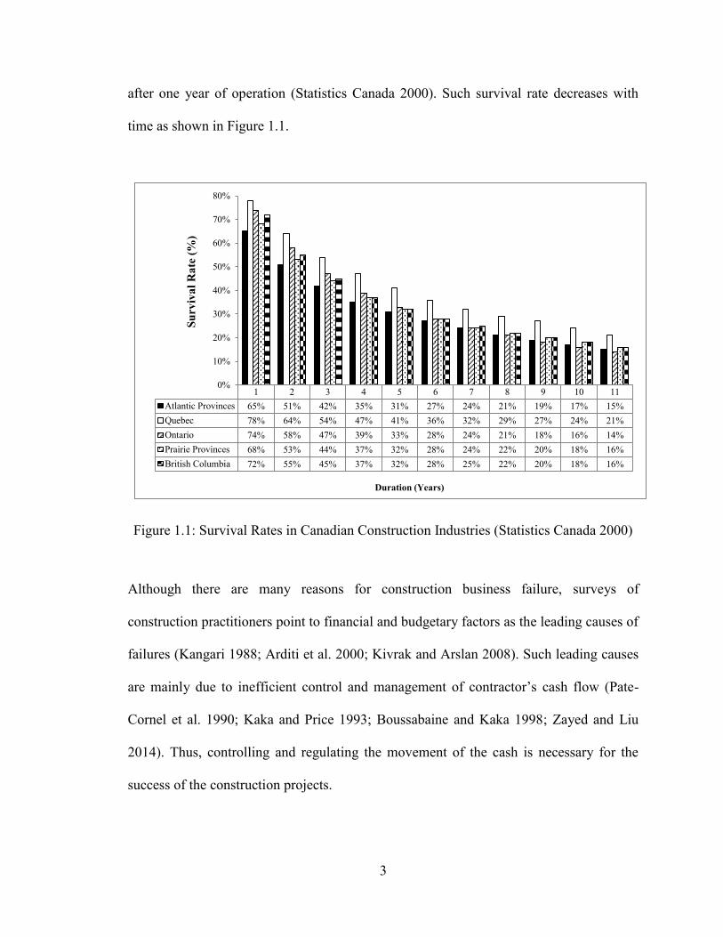
Figure 1.1: Survival Rates in Canadian Construction Industries (Statistics Canada 2000) ............. 3
Figure 1.2: Summary of Research Methodology ............................................................................. 8
Figure 2.1: Illustration of Project Time/Cost Tradeoff (Hegazy 1999b) ....................................... 12
Figure 2.2: Resource Usage Patterns ............................................................................................. 14
Figure 2.3: Illustration of Resource-Constrained Scheduling ........................................................ 15
Figure 2.4: Types of Resource Fluctuations (El-Rayes and Jun 2009) .......................................... 17
Figure 2.5: Calculations of the New Metrics (El-Rayes and Jun 2009) ......................................... 19
Figure 2.6: Difference Between RRH and RID Metrics (El-Rayes and Jun 2009) ....................... 21
Figure 2.7: Cash Flow of a Typical Construction Project (Abido and Elazouni 2010) ................. 23
Figure 2.8: Illustration of the Crowding Distance Calculation (Deb et al. 2002) .......................... 48
Figure 2.9: NSGA-II Process ......................................................................................................... 49
Figure 2.10: Example of Non-dominated Sorting Procedure......................................................... 51
Figure 2.11: Example of Tournament Selection without Replacement ......................................... 54
Figure 2.12: Example of One-Point Crossover .............................................................................. 55
Figure 2.13: Example of Selective Mutation ................................................................................. 56
Figure 2.14: Classification of Common Optimization Methods .................................................... 60
Figure 2.15: Classification of Common Meta-heuristics ............................................................... 63
Figure 3.1: Research Methodology Flowchart ............................................................................... 67
Figure 3.2: Twenty-Activity Project Network (El-Rayes and Jun 2009) ....................................... 77
Figure 3.3: Twenty-Activity Project Initial Resource Profile (El-Rayes and Jun 2009) ............... 77
Figure 3.4: Twenty-Activity Project Minimum Resource Profile (El-Rayes and Jun 2009) ......... 79
Figure 3.5: Decision Variables and Optimization Objectives ........................................................ 84
Figure 3.6: Model Formulation Summary ..................................................................................... 88
Figure 4.1: Model Overview .......................................................................................................... 93
Figure 4.2: Initial Scheme .............................................................................................................. 95
Figure 4.3: Extension Scheme ....................................................................................................... 95
Figure 4.4: Chromosome Structure Representation ....................................................................... 96
Figure 4.5: Example of Illegal Offspring from Crossover ............................................................. 99
Figure 4.6: CPM Network of a 13-Activity Project ....................................................................... 99
Figure 4.7: Seven-day Extension of the 13-Activity Project ....................................................... 100
Figure 4.8: Improved Crossover Operator – Forward Path.......................................................... 103
Figure 4.9: Improved Crossover Operator – Backward Path ....................................................... 104
Figure 4.10: Improved Mutation Operator ................................................................................... 105
Figure 4.11: Model Development Framework ............................................................................. 106
Figure 5.1: Pareto-optimal Time/Cost Tradeoff Curve for Test (1) ............................................. 117
Figure 5.2: Pareto-optimal Time/Cost Tradeoff Curves for Test (2) ........................................... 121
Figure 5.3: Twelve-Activity Project Network ............................................................................. 122
Figure 5.4: Two-Objectives Optimization Tradeoff Curves ........................................................ 131
xi
Figure 5.5: Five-Objectives Optimization Results (Case Study 1) .............................................. 139
Figure 5.6: RC-PR-RID1 Tradeoff Surface Plot .......................................................................... 140
Figure 5.7: RC-PR-RID2 Tradeoff Surface Plot .......................................................................... 141
Figure 5.8: RC-PR-RID3 Tradeoff Surface Plot .......................................................................... 141
Figure 5.9: 25-Activity Project CPM Network ............................................................................ 143
Figure 5.10: 30-Activity Project CPM Network .......................................................................... 143
Figure 5.11: 25-Activity Project Initial Schedule (Mode 1) ........................................................ 147
Figure 5.12: 30-Activity Project Initial Schedule (Mode 1) ........................................................ 148
Figure 5.13: Initial Net Cash Flow (Mode 1)............................................................................... 153
Figure 5.14: Net Cash Flows Comparison ................................................................................... 156
Figure 5.15: Resource Demand Profiles Comparison .................................................................. 157
Figure 5.16: RC-PR-RFPD Tradeoff Surface Plot (Case Study 2) .............................................. 158
Figure 5.17: RC-PR-RFPD Tradeoff Surface Plot with Extension (Case Study 2) ..................... 159
Figure 5.18: Effect of Applying Extension Increment on the Net Cash Flow ............................. 161
Figure 5.19: RC-PR-RFPD Tradeoff Surface Plot (Case Study 3) .............................................. 164
Figure 5.20: RC-PR-RFPD Tradeoff Surface Plot with Extension (Case Study 3) ..................... 165
Figure 6.1: Application Architecture (Johnson Technology Systems 2014) ............................... 169
Figure 6.2: Parallel Computing Concept ..................................................................................... 172
Figure 6.3: MOSCOPEA Development Framework ................................................................... 176
Figure 6.4: Relational Database Design....................................................................................... 177
Figure 6.5: MOSCOPEA Welcome Window .............................................................................. 178
Figure 6.6: Window (A) ............................................................................................................... 180
Figure 6.7: Window (B) ............................................................................................................... 181
Figure 6.8: Create New Solution ................................................................................................. 182
Figure 6.9: Identify Activities and Precedence Relationship ....................................................... 183
Figure 6.10: Identify Resource Utilization Modes....................................................................... 183
Figure 6.11: Full Identified Data for an Activity Sample ............................................................ 184
Figure 6.12: General Data (Panel 2A) ......................................................................................... 185
Figure 6.13: Time Parameters (Panel 3A) ................................................................................... 185
Figure 6.14: Financial Parameters (Panel 4A) ............................................................................. 186
Figure 6.15: Contract Terms (Panel 5A) ...................................................................................... 186
Figure 6.16: Projects Data Status (Panel 8A) .............................................................................. 187
Figure 6.17: Optimize and Assign Output Folder ........................................................................ 188
Figure 6.18: Analysis Progress Bar ............................................................................................. 189
Figure 6.19: Optimal Tradeoffs Output ....................................................................................... 190
Figure 6.20: Bar Chart Output ..................................................................................................... 191
Figure 6.21: Activities’ Details Output ........................................................................................ 191
Figure 6.22: Cash Flow Details Output ....................................................................................... 192
Figure 6.23: Resource Profile Output .......................................................................................... 192

xii
LIST OF TABLES
Table 1.1: U.S. Contractors’ Failure Rate (Surety Information Office 2012) ................................. 2
Table 3.1: Direct Costs (Experiment 1) ......................................................................................... 75
Table 3.2: Time, Financial, and Contractual Data (Experiment 1) ................................................ 76
Table 3.3: Direct Costs (Experiment 2) ......................................................................................... 78
Table 3.4: Time, Financial, and Contractual Data (Experiment 2) ................................................ 78
Table 3.5: Effect of Minimizing Resource Fluctuations ................................................................ 80
Table 5.1: Data for Test (1) (adapted from Feng et al. 1997) ...................................................... 114
Table 5.2: Optimum Solutions for Test (1) .................................................................................. 116
Table 5.3: Data for Test (2) (adapted from Leu and Yang 1999) ................................................ 118
Table 5.4: Optimum Solutions for Test (2) – Unconstrained Resource ....................................... 120
Table 5.5: Optimum Solutions for Test (2) – Constrained Resource ........................................... 120
Table 5.6: Optimum Solutions for Test (3) .................................................................................. 123
Table 5.7: Financial and Contractual Data (Case Study 1) .......................................................... 125
Table 5.8: Single-Objective Optimization Results (Case Study 1) .............................................. 126
Table 5.9: Two-Objectives Optimization Results (Case Study 1) ............................................... 130
Table 5.10: Set of Non-Conflicting Objectives ........................................................................... 132
Table 5.11: Main-Tradeoff Combination Sets ............................................................................. 133
Table 5.12: Main and Sub-Tradeoff Combination Sets ............................................................... 134
Table 5.13: Five-Objectives Remarkable Solutions (Case Study 1) ............................................ 137
Table 5.14: Summary of Optimization Results (Case Study 1) ................................................... 142
Table 5.15: Time, Financial, and Contractual Data (Case Study 2) ............................................ 144
Table 5.16: Cost and Resource Data (25-Activity Project).......................................................... 145
Table 5.17: Cost and Resource Data (30-Activity Project).......................................................... 146
Table 5.18: Initial Objectives’ Values (25-30 Activity Projects) ................................................ 146
Table 5.19: Initial Weekly Cash Outflow and Inflow Calculations (Mode 1) ............................. 151
Table 5.20: Initial Financial Parameters Calculations (Mode 1) ................................................. 152
Table 5.21: Single-Objective Optimization Results (Case Study 2) ............................................ 154
Table 5.22: Three-Objectives Remarkable Solutions (Case Study 2) .......................................... 154
Table 5.23: Three-Objectives Remarkable Solutions with Extension (Case Study 2) ................. 159
Table 5.24: Summary of Optimization Results (Case Study 2) ................................................... 160
Table 5.25: Time, Financial, and Contractual Data (Case Study 3) ............................................ 162
Table 5.26: Initial Objectives’ Values (100-120 Activity Projects) ............................................ 163
Table 5.27: Single-Objective Optimization Results (Case Study 3) ............................................ 163
Table 5.28: Three-Objectives Remarkable Solutions (Case Study 3) .......................................... 164
Table 5.29: Three-Objectives Remarkable Solutions with Extension (Case Study 3) ................. 165
Table 5.30: Summary of Optimization Results (Case Study 3) ................................................... 166
Table A.1: Precedence Relation, Cost, and Resource Data ......................................................... 221
Table A.2: Time, Financial, and Contractual Data ...................................................................... 222
Table A.3: Schedule Sample of P1-G1.......................................................................................... 222

xiii
Table A.4: Parent Population of First Generation (P-G1) ............................................................ 223
Table A.5: Non-Domination Ranking of P-G1 ............................................................................. 226
Table A.6: Mating Pool................................................................................................................ 229
Table A.7: Child Population of First Generation (Q-G1) ............................................................. 229
Table A.8: Combined Population of First Generation (R-G1) ..................................................... 230
Table A.9: Non-Domination Ranking of R-G1 ............................................................................ 231

xiv
LIST OF ACRONYMS
BFF Backward Free Float
C# C Sharp Programming Language
CL Credit Limit
CP Constrained Programming
CPM Critical Path Method
DP Dynamic Programming
FC Financing Cost
FFF Forward Free Float
GAs Genetic Algorithms
GUI Graphical User Interface
IP Integer Programming
LP Linear Programming
MOEAs Multi-Objective Evolutionary Algorithms
MOP Multi-objective Optimization
MOSCOPEA Multi-Objective SCheduling OPtimization using Evolutionary Algorithm
MRD Maximum Resource Demand
MPI Message Passing Interface
NSGA Non-dominated Sorting Genetic Algorithm
NSGA-II Elitist Non-dominated Sorting Genetic Algorithm
PR Profit
RC Required Credit
RFPD Resource Fluctuation and Peak Demand
RID Resource Idle Days
RL Resource Limit
RRH Release and Re-Hire
RWGA Random Weighted Genetic Algorithm
SPEA Strength Pareto Evolutionary Algorithm
SPEA-II Improved Strength Pareto Evolutionary Algorithm

xv
TC Total Cost
TCT Time Cost Tradeoff
TD Total Duration
VEGA Vector Evaluated Genetic Algorithm
WBGA Weighted-Based Genetic Algorithm

1
CHAPTER 1: INTRODUCTION
The capability to timely obtain sufficient cash is considered one of the most common and
critical challenges that contractors usually face during the execution of any construction
project. As a result, cash must be thought of as a limited resource because its
procurement has always been the first concern of contractors. During any project period,
contractors never carry out any work that has no cash availability despite the commitment
to stick to schedules. This clear principle of operation makes the establishment of a
balance between financing needs and available cash, along the project’s duration, a very
vital concept to produce realistic schedules. Should sufficient cash not be available,
delays in project completion times are anticipated which result in increased overheads
and decreased profits. Therefore, a sound and well managed project finance-based
scheduling model should be established in order to allow the contractor to identify his/her
cash needs during each period of the constructed project(s).
Since the execution of construction projects demands huge investments, contractors
rarely rely on their own savings to carry out projects (Elazouni and Metwally 2005).
Usually, contractors procure an external source of financing to cover the cash deficit.
Loans, line of credits, leases, trade financing, and credit cards are the most common
financing instruments used in construction industry (Fathi and Afshar 2010). One of the
prevalent methods of financing construction projects is line of credit which allows
contractors to withdraw cash up to a specified credit limit. When a line of credit is
available to the contractor; projects’ schedules should be devised under cash constraint of

2
the credit limit to maximize the predicted profit, maximize the utilization of cash flow at
the company level, and satisfy each project’s constraints.
1.1 RESEARCH MOTIVATION AND PROBLEM STATEMENT
Construction industry is considered as one of the most risky sectors due to high level of
uncertainties in their nature. Every year thousands of contractors face bankruptcy and
business failure. According to a relatively recent study made by the marketing research
firm “BizMiner”, of the 918,483 U.S. general contractors and operative builders, heavy
construction contractors, and special trade contractors operating in 2010, only 696,441
were still in business in 2012 resulting in a 24.2% failure rate (Surety Information Office
2012). This failure was not only from the year 2010 to 2012, but according to the
reachable sources, this significant failure rate goes back from the year 2002 as shown in
Table 1.1. Moreover, it was stated that only 47% of the U.S. startup businesses in
construction are still operating after four years (Statistic Brain 2014).
Table 1.1: U.S. Contractors’ Failure Rate (Surety Information Office 2012)
In Business Survivors Failure Rate
Year No. of Contractors Year No. of Contractors
2002 853,372 2004 610,357 28.5%
2004 850,029 2006 649,602 23.6%
2006 1,155,245 2008 919,848 20.4%
2009 897,602 2011 702,618 21.7%
2010 918,483 2012 696,441 24.2%
Similarly, the Canadian construction industry suffers from significant failure rates as it
was reported that around 65 to 78% of startup construction businesses in Canada survived
3
1 2 3 4 5 6 7 8 9 10 11
Atlantic Provinces 65% 51% 42% 35% 31% 27% 24% 21% 19% 17% 15%
Quebec 78% 64% 54% 47% 41% 36% 32% 29% 27% 24% 21%
Ontario 74% 58% 47% 39% 33% 28% 24% 21% 18% 16% 14%
Prairie Provinces 68% 53% 44% 37% 32% 28% 24% 22% 20% 18% 16%
British Columbia 72% 55% 45% 37% 32% 28% 25% 22% 20% 18% 16%
0%
10%
20%
30%
40%
50%
60%
70%
80%S
urv
iva
l R
ate
(%
)
Duration (Years)
after one year of operation (Statistics Canada 2000). Such survival rate decreases with
time as shown in Figure 1.1.
Figure 1.1: Survival Rates in Canadian Construction Industries (Statistics Canada 2000)
Although there are many reasons for construction business failure, surveys of
construction practitioners point to financial and budgetary factors as the leading causes of
failures (Kangari 1988; Arditi et al. 2000; Kivrak and Arslan 2008). Such leading causes
are mainly due to inefficient control and management of contractor’s cash flow (Pate-
Cornel et al. 1990; Kaka and Price 1993; Boussabaine and Kaka 1998; Zayed and Liu
2014). Thus, controlling and regulating the movement of the cash is necessary for the
success of the construction projects.

4
Financial management has long been recognized as an important management tool and
proper cash flow management is crucial to the survival of a construction company
because cash is the most important corporate resource for its day-to-day activities (Peer
1982). However, contractors mainly deal with the project scheduling and financing as
two independent functions of construction project management. The absence of the
required linkage between those two functions resulted in devising non-executable
schedules which lead to a high volume of project failure due to finance deficit. It has
been reported that the lack of finance experience comprised 77 to 95% of the total
contractors' failures during 30-year period (Russell 1991). Other consequences of the
absence of the required linkage includes; fund has inefficiently been utilized because
projects' schedules were devised separately without considering the overall liquidity
situation of contractors' portfolios, the substantial finance cost has been omitted which
has eaten up contractors' profit, and eventually the whole purpose behind scheduling has
been defeated to a certain extent.
Several studies were carried to integrate project scheduling along with available finance
in order to achieve project’s objectives. This integration is known as “finance-based
scheduling” which re-schedules the projects’ activities without violating specified
project’s constraints to achieve company’s objectives. These objectives focused on
minimizing the total project duration, financing costs, and maximum required credit
while maximizing the profit. However, there is a lack of research that considers
integrating resource management techniques including resource leveling and resource
allocation simultaneously with the finance-based scheduling concept. Considering those

5
two aspects together have a significant impact on many areas of project management
including time, cost, resource, and risk. Moreover, few researches solved the finance-
based scheduling problem considering the contractor’s entire portfolio rather than single
project. Multiple concurrent projects involves sharing and competing for limited
resources such as funds, equipment, manpower and other resources among different
projects, which increases the complexity of the scheduling process. The allocation of
scarce resources then becomes a major objective of the problem. In such cases, planners
are generally concerned with a number of different decision criteria, often conflicting
among each other, according to their importance and priorities.
1.2 RESEARCH OBJECTIVES
The main objective of this research is to develop a multi-objective scheduling
optimization model for multiple projects considering resource leveling and allocation
together with projects’ financing. The model aims to solve for enterprises problems of
prioritizing projects under resource-conflict conditions, allocating limited resources, and
optimizing all the projects’ multi-objectives under certain funding limits. This is done by
producing optimal/near optimal tradeoffs between different selected projects’ objectives
including duration, total cost, financing cost, required credit, profit, and resource
fluctuations. The model takes into account projects’ activities to have one or more
resource utilization mode with multi-resources. In order to achieve the stated main
objective; the following sub-objectives are to be attained:
1. Develop scheduling, resource, and cash flow models for multiple construction
projects.

6
2. Integrate the aforementioned management models to formulate and develop a
multi-objective scheduling optimization model for multiple projects.
3. Implement, test, and automate the developed optimization model.
1.3 SUMMARY OF RESEARCH METHODOLOGY
As shown in Figure 1.2, the methodology of this research can be summarized as follows:
1. Literature review is performed which involves identifying previous research
efforts made by different researchers to solve the finance-based scheduling,
time/cost tradeoff, resource leveling, and resource allocation problems. In
addition, a survey of different multi-objective techniques used to solve such
problems is reviewed.
2. Three main management models are developed, namely: (1) scheduling model
that establishes optimal/near optimal schedules for construction projects; (2)
resource model to calculate the resource fluctuations and maximum daily
resource demand; and (3) cash flow model to calculate projects’ cash flow
parameters.
3. Model formulation is established to convert the basic multi-objective and their
constraints into a mathematical model. The objectives involves minimizing the
duration of multiple projects, total cost, financing cost, maximum required credit,
and resource fluctuations and maximizing the profit. On other hand, the
constraints set to achieve those objectives are: (1) dependencies between
projects’ activities are to be fulfilled; (2) credit limit not to be exceeded; and (3)
daily resource limit not to be exceeded.

7
4. Multi-objective scheduling optimization model is developed using NSGA-II to
optimize the projects’ objectives under specified constraints. The model performs
genetic algorithms operations in three main phases: (1) population initialization;
(2) fitness evaluation; and (3) generation evolution.
5. The developed model is tested and implemented using different case studies
obtained from literature to prove its validity and ability to optimize such
problems successfully and efficiently.
6. An automated tool using C# language is built with a friendly graphical user
interface to facilitate solving multi-objective scheduling optimization problems
for contractors and practitioners.
7. Finally, the conclusions and contributions achieved from this research is
summarized as well as the suggested recommendations for future work.

8
START
LITERATURE
REVIEW
Time/Cost Tradeoff
Resource Leveling
and AllocationApplied Techniques
Finance-Based
Scheduling
MODEL IMPLEMENTATION AND TESTING
Model
Successful?
Yes
No
MODEL FORMULATION
Decision Variables Objectives Constraints
DEVELOP MANAGEMENT MODELS
Cash Flow Model
Scheduling Model
Resource Model
MULTI-OBJECTIVE SCHEDULING
OPTIMIZATION MODEL DEVELOPMENT
AUTOMATED TOOL
(MOSCOPEA)
END
CONCLUSIONS &
RECOMMENDATIONS
Figure 1.2: Summary of Research Methodology

9
1.4 THESIS ORGANIZATION
This thesis consists of seven chapters. Chapter 1 includes the research motivations and
problem statement, research objectives, and summary of the research methodology.
Chapter 2 involves a detailed literature review on the previous attempts carried by
different researchers to solve the finance-based scheduling, time/cost tradeoff, resource
leveling, and resource allocation problems. In addition it involves a brief review on the
different used optimization techniques and a detailed review on the elitist non-dominated
sorting genetic algorithm (NSGA-II) technique. Chapter 3 provides a detailed description
of the research methodology. Chapter 4 explains in details the multi-objective scheduling
optimization model development process. Chapter 5 shows the testing and
implementation results and analysis of the developed optimization model. Chapter 6
presents the built automated tool for the developed model. Finally, Chapter 7 summarizes
the research conclusions and contributions, and discusses its limitations and suggested
recommendations for future work.
10
CHAPTER 2: LITERATURE REVIEW
Optimization problems in construction scheduling are traditionally classified, depending
on their objective, into one of the following: (1) time/cost tradeoff; (2) resource
allocation; or (3) resource leveling. Time/cost tradeoff is concerned with minimizing the
direct cost while meeting a desired completion time (Hegazy 1999b). Resource allocation
fulfills constraints on resource with the minimum increase in project duration (Hegazy
1999a). Resource leveling is concerned with minimizing peak resource requirements and
period-to-period fluctuations in resource usage while maintaining the original project
duration (Moselhi and Lorterapong 1993).
This chapter is divided into seven sections. The first two sections include brief reviews of
time/cost tradeoff analysis and resource management techniques including the resource
allocation and resource leveling. The third section describes in detail the concept and
technique of finance-based scheduling. The fourth section reviews research work in the
literature related to the utilization of single and multiple-objective optimization
techniques to solve scheduling problems. In addition, the fourth section reviews the
research efforts related to usage of optimization techniques to solve scheduling problems
of multiple projects within a portfolio. The fifth section reviews a background on the
multi-objective evolutionary algorithms focusing in the sixth section on the fast non-
dominated sorting genetic algorithm (NSGA-II) as an optimization technique. Finally, the
seventh section summarizes the findings and limitations of the literature.

11
2.1 TIME/COST TRADEOFF ANALYSIS
Time/Cost Tradeoff (TCT) is defined as a process to identify suitable construction
activities for speeding up, and for deciding ‘by how much’ so as to attain the best
possible savings in both time and cost (Eshtehardian et al. 2008). It is a technique used to
overcome critical path method's (CPM) lack of ability to confine the schedule to a
specified duration (Hegazy and Menesi 2012). The objective of the analysis is to reduce
the original CPM duration of a project in order to meet a specific deadline with the
minimum cost (Chassiakos and Sakellaropoulos 2005). TCT analysis is an important
management tool because it can also be used to accelerate a project so that delays can be
recovered and liquidated damages avoided. The project can be accelerated through the
addition of resources, e.g., labor or equipment, or through the addition of work hours to
crash critical activities. Reducing project duration therefore results in an increase in direct
costs, e.g., the cost of materials, labor, and equipment. However, the increase in direct
cost expenditures can be justified if the indirect costs, e.g., expenditures for management,
supervision, and inspection, are reduced or if a bonus is earned (Gould 2005).
TCT analysis involves selecting some of the critical activities in order to reduce their
duration through the use of a faster construction method, even at an additional cost.
Different combinations of construction methods for the activities can then be formed,
each resulting in a specific project duration and direct cost. To determine the optimum
TCT decision for a project, the direct cost and indirect cost curves are plotted
individually so that the total cost curve can be developed from the addition of these two
components, as shown in Figure 2.1. The minimum point on the total cost curve

12
represents the set of optimum combination of construction methods for the activities.
However, for projects involving large number of activities with varying construction
options, finding optimal TCT decisions becomes difficult and time consuming (Zheng et
al. 2004).
Figure 2.1: Illustration of Project Time/Cost Tradeoff (Hegazy 1999b)
2.2 RESOURCE MANAGEMENT
Traditionally, resource management problems in construction projects have been solved
either as a resource leveling or as a resource allocation problem (Wiest and Levy 1969;
Antill and Woodhead 1982; Moder et al. 1983). The objective in the resource leveling
problem is to reduce peak resource requirements and smooth out period-to-period
resource usage within the required project duration, with the premise of unlimited
resource availability (Chan et al. 1996). The resource allocation arises when there are
definite limits on the amount of resources available. The scheduling objective is to extend

13
the project duration as minimum as possible beyond the original critical path duration in
such a way that the resource constraints are met. In this process, both critical and
noncritical activities are shifted (Senouci and Adeli 2001).
2.2.1 Resource Leveling
The resource leveling problem arises when there are sufficient resources available and it
is necessary to reduce the fluctuations in the resource usage over the project duration.
The objective of the leveling process is to “smooth” resource usage profile of the project
without elongating the project duration as much as possible. This is accomplished by
rescheduling of activities within their available slack to give the most acceptable profiles
(Davis 1973). In resource leveling, the project duration of the original critical path
remains unchanged.
Fluctuations of resources as shown in Figure 2.2a are undesirable for the contractor. It is
expensive to hire and fire labor on a short term basis to satisfy fluctuating resource
requirements. The short term hiring and firing presents labor, utilization, and financial
difficulties because (1) the costs for employee processing are increased; (2) top-notch
journeymen are discouraged to join a company with a reputation of doing this; and (3)
new, less experienced employees require long periods of training (Senouci and Adeli
2001). As a result, the scheduling objective of the resource leveling problem is to make
the resource requirements as uniform as possible (Figure 2.2b) or to make them match a
particular non-uniform resource distribution in order to meet the needs of a given project
(Figure 2.2c).

14
Therefore, efficient use of project resources will decrease construction costs to owners
and consumers, and at the same time, will increase contractor’s profits (Hegazy and
Kassab 2003). In other words, alternative labor utilization strategies and better utilization
of existing labor resources are needed to improve work productivity and reduce
construction costs.
Figure 2.2: Resource Usage Patterns
0
10
20
30
40
0 5 10 15 20 25 30
Nu
mb
er o
f R
eso
urc
es
/ d
ay
Workdays
(b) Constant
0
10
20
30
40
0 5 10 15 20 25 30Nu
mb
er o
f R
eso
urc
es /
da
y
Workdays
(a) Fluctuating
0
10
20
30
40
0 5 10 15 20 25 30
Nu
mb
er o
f R
eso
urc
es
/ d
ay
Workdays
(c) Varying

15
2.2.2 Resource Allocation
Resource allocation attempts to reschedule a project’s activities so that a limited number
of resources can be efficiently utilized while keeping the unavoidable extension of the
project to a minimum (Hegazy 1999a). A simple illustration for a project’s initial
resource profile in which resource limit was exceeded is shown in Figure 2.3a. On the
other hand, Figure 2.3b shows the rescheduled project’s resource profile where the
resource limit is kept at or below the maximum limit, however, the initial duration was
exceeded.
Figure 2.3: Illustration of Resource-Constrained Scheduling
0
1
2
3
4
1 2 3 4 5 6 7 8Nu
mb
er o
f R
esou
rces
/ d
ay
Workdays
(a) Initial Resource Profile
0
1
2
3
4
1 2 3 4 5 6 7 8 9 10
Nu
mb
er o
f R
eso
urc
es /
day
Workdays
(b) Rescheduled Resource Profile
Max Resource Limit = 2
Max Resource Limit = 2
16
The focus of scheduling in these situations is to prioritize and allocate resources in such a
manner that there is minimal project delay. Beside the importance of ensuring that the
resource limit is not exceeded; the logical relationships between the activities of a project
network should simultaneously be preserved. Resource allocation problems can be
classified into single-mode resource allocation and multi-mode resource allocation when
there is more than one alternative for activity duration and resource requirement.
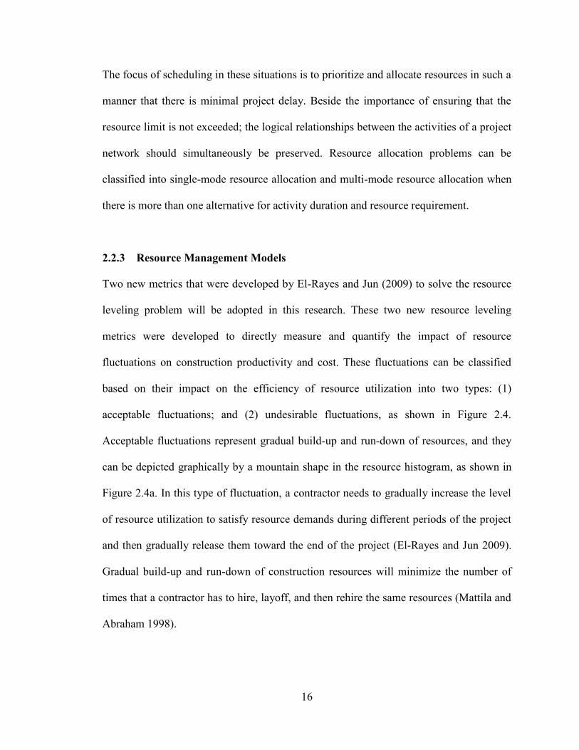
2.2.3 Resource Management Models
Two new metrics that were developed by El-Rayes and Jun (2009) to solve the resource
leveling problem will be adopted in this research. These two new resource leveling
metrics were developed to directly measure and quantify the impact of resource
fluctuations on construction productivity and cost. These fluctuations can be classified
based on their impact on the efficiency of resource utilization into two types: (1)
acceptable fluctuations; and (2) undesirable fluctuations, as shown in Figure 2.4.
Acceptable fluctuations represent gradual build-up and run-down of resources, and they
can be depicted graphically by a mountain shape in the resource histogram, as shown in
Figure 2.4a. In this type of fluctuation, a contractor needs to gradually increase the level
of resource utilization to satisfy resource demands during different periods of the project
and then gradually release them toward the end of the project (El-Rayes and Jun 2009).
Gradual build-up and run-down of construction resources will minimize the number of
times that a contractor has to hire, layoff, and then rehire the same resources (Mattila and
Abraham 1998).

17
Figure 2.4: Types of Resource Fluctuations (El-Rayes and Jun 2009)
On the other hand, undesirable fluctuations represent temporary decreases in the demand
for construction resources. This can be depicted graphically by a valley shape in the
resource histogram as shown in Figure 2.4b. In this type of fluctuation, a contractor is
forced to either: (1) release the additional construction resources and rehire them at a later
stage when needed or (2) retain the idle construction resources on site until they are
needed later in the project (El-Rayes and Jun 2009). In order to generate productive and
cost effective construction schedule, this undesirable fluctuation should be directly
measured and minimized. To accomplish this, two new resource leveling metrics were
developed: (1) Release and Re-Hire (RRH); and (2) Resource Idle Days (RID) (El-Rayes
and Jun 2009).
2.2.3.1 Release and Re-Hire (RRH)
This metric is designed to quantify the total amount of resources that need to be
temporarily released during low demand periods and rehired at a later stage during high

18
demand periods, as shown in Figure 2.5b. The present model utilizes Equation 2.1 to
calculate the RRH metric in three sequential steps: (1) calculate the total daily resource
fluctuations (HR) using Equation 2.2 which sums up all the increases and decreases in the
daily resource demand, as shown in Figure 2.5b; (2) identify the total increases in the
daily resource demand (H) which is half the total daily resource fluctuations (HR); (3)
determine the number of released and rehired resources by subtracting the maximum
resource demand (MRD) from the total increases in the daily resource demand (H), as
shown in Equation 2.1.
RRH = H – MRD = ((1/2) x HR) – MRD …………………………………….….…....(2.1)
𝐻𝑅 = [𝑟1 + ∑ |𝑟𝑡 − 𝑟𝑡+1| + 𝑟𝑇𝑇−1𝑡=1 ] ………………………………………………...….(2.2)
MRD = Max (r1, r2, ….., rT) …………………………………………………….....….(2.3)
Where; RRH = total amount of resources that need to be temporarily released and rehired
during the entire project duration; H = total increases in the daily resource demand; HR =
total daily resource fluctuations; T = total project duration; rt = resource demand on day
(t); rt+1 = resource demand on day (t + 1); and MRD = maximum resource demand during
the entire project duration. It should be noted that the RRH metric can be practical and
useful in projects that allow the release and rehire of construction workers. In other
projects that restrict this type of resource release and rehire, contractors are often required
to keep the additional resources idle on site during low demand periods, as shown in

19
Figure 2.5b. To quantify and minimize the impact of this decision on construction
productivity and cost, the following section presents the development of the new metric
named RID.
Figure 2.5: Calculations of the New Metrics (El-Rayes and Jun 2009)
2.2.3.2 Resource Idle Days (RID)
This metric is designed to quantify the total number of idle and nonproductive resource
days caused by undesirable resource fluctuations and it can be calculated using Equation
2.4. As shown in Figure 2.5c, idle resources occur on day (t) when the resource demand
on that day (t) dips to a lower level than the peak demand levels experienced prior to and
after that day (t). When this dip in resource demand occurs, the idle resources on day (t)
can be calculated by subtracting its resource level from the least of the peak demands that
occur before or after that day as shown in Figure 2.5c. For example, the number of idle
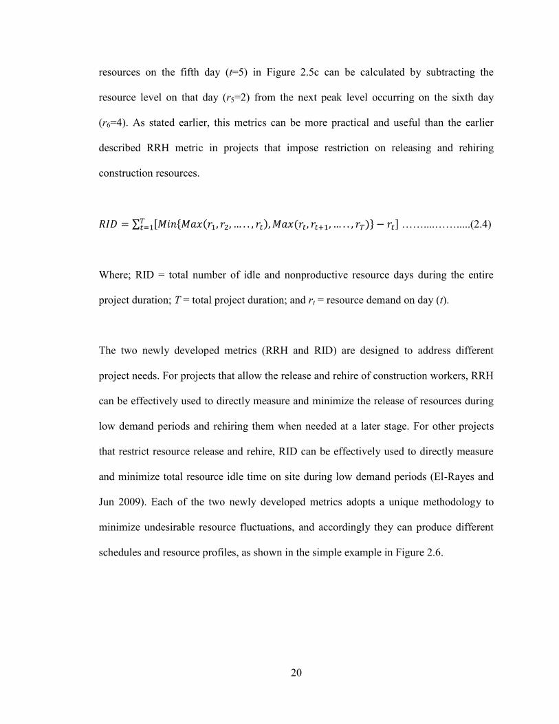
20
resources on the fifth day (t=5) in Figure 2.5c can be calculated by subtracting the
resource level on that day (r5=2) from the next peak level occurring on the sixth day
(r6=4). As stated earlier, this metrics can be more practical and useful than the earlier
described RRH metric in projects that impose restriction on releasing and rehiring
construction resources.
𝑅𝐼𝐷 = ∑ [𝑀𝑖𝑛{𝑀𝑎𝑥(𝑟1, 𝑟2, … . . , 𝑟𝑡), 𝑀𝑎𝑥(𝑟𝑡, 𝑟𝑡+1, … . . , 𝑟𝑇)} − 𝑟𝑡]𝑇𝑡=1 ……....…….....(2.4)
Where; RID = total number of idle and nonproductive resource days during the entire
project duration; T = total project duration; and rt = resource demand on day (t).
The two newly developed metrics (RRH and RID) are designed to address different
project needs. For projects that allow the release and rehire of construction workers, RRH
can be effectively used to directly measure and minimize the release of resources during
low demand periods and rehiring them when needed at a later stage. For other projects
that restrict resource release and rehire, RID can be effectively used to directly measure
and minimize total resource idle time on site during low demand periods (El-Rayes and
Jun 2009). Each of the two newly developed metrics adopts a unique methodology to
minimize undesirable resource fluctuations, and accordingly they can produce different
schedules and resource profiles, as shown in the simple example in Figure 2.6.

21
Figure 2.6: Difference Between RRH and RID Metrics (El-Rayes and Jun 2009)
While existing metrics attempt to transform fluctuating resource profile to a
predetermined desirable shape (e.g., a rectangular or a parabolic), the new metrics focus
on minimizing only undesirable fluctuation, and accordingly they are capable of
generating more efficient resource utilizations than existing ones (El-Rayes and Jun
2009).
2.3 FINANCE-BASED SCHEDULING
Establishing bank overdrafts has been one of the prevalent methods of financing
construction projects (Ahuja 1976). Finance-based scheduling enables producing
schedules that correspond to overdrafts of desired credit limits. Control of the credit limit
of an overdraft provides many benefits including negotiating lower interest rates with
bankers, setting favorable terms of repayment, and reducing penalties incurred for any
unused portions of overdraft cash (Elazouni and Gab-Allah 2004). In addition, the ability
to adjust credit limits helps contractors avoid the phenomenon of progressive cash deficit.

22
This situation occurs when cash available in a given month does not allow the scheduling
of much work. During the next month, when a reimbursement is expected, the generated
income allows scheduling less work and so forth (Elazouni and Gab-Allah 2004).
Typically, an additional cost component for financing is associated with the cash
procurement through the banks’ credit lines. Contractors normally deposit owners’
progress payments into the credit-line accounts to continually reduce the outstanding
debit and consequently the financing costs (Abido and Elazouni 2010). As the cash flow
shown in Figure 2.7 indicates; contractors charge the expenses caused by labor,
equipment, materials, subcontractors, and other indirect costs (cash outflow Et) against,
and deposit progress payments (cash inflow Pt) into the credit-line accounts. In practice,
it can be reasonably assumed that these transactions occur as of the cut-off times between
periods (Abido and Elazouni 2010). Accordingly, the values of the outstanding debt (Ft)
as of the cut-off times are determined. The financing costs as of the cutoff times are
determined by applying the prescribed interest rate to the outstanding debt. The
summations of the values of the outstanding debt and the accumulated financing costs
(I’t) constitute the negative cumulative balance (F’t). The cumulative net balance value
(N’t) constitutes the negative cumulative balances after depositing the progress payments.
The cumulative net balance of all Et, Pt, and I’t transactions constitutes the profit as of the
end of the project (Abido and Elazouni 2010).

23
Figure 2.7: Cash Flow of a Typical Construction Project (Abido and Elazouni 2010)
Another concern of financing, though more important than the incorporation of financing
costs, constitutes the credit-limit constraints imposed on the credit lines (Abido and
Elazouni 2010). The credit limit specifies the maximum value the negative cumulative
balance as of the cutoff times are allowed to reach. Thus, finance-based scheduling
achieves the desired integration between scheduling and financing by incorporating
financing costs into the project total cost as well as scheduling activities such that the
values of the negative cumulative balance as of the cutoff times never exceeds the
specified credit limit (Abido and Elazouni 2010). The techniques employed to devise
finance-based schedules normally fulfill this financial constraint with the objectives of
minimizing the financing costs and maximizing the contractor’s profit.
Being an aspect of the whole corporate rather than the individual projects, contractors
manage the financing aspect at the corporate level. In other words, contractors' concern is
generally to timely procure cash for all ongoing projects (Abido and Elazouni 2011).
Finance-based scheduling in this context ensures that the resulting values of the negative
cumulative balances of all projects do not add up to exceed the credit limit, whereas the

24
positive cumulative balances that occur in some projects are utilized to schedule activities
of some other projects. This ensures that scheduling concurrent projects can be related to
the overall liquidity situation of contractors. The sole objective of maximizing the profit
of a single project is changed in this context to the objective of maximizing the profit
value of all ongoing projects. Finance-based scheduling techniques schedule projects'
activities such that the total profit of the projects is maximized while the financial
constraint is fulfilled.
2.3.1 Cash Flow Model
The equations in this subsection are presented conforming to the financial terminology
used by Au and Hendrickson (1986). Let direct cost disbursements of all activities
performed on day i be denoted by yi; this is referred to as project direct cost disbursement
of day i. Thus yi can be calculated as follows:
𝑦𝑖 = ∑ (𝑦𝑝𝑖 )𝑛𝑖𝑝=1 i = 1 ,2 ,…..D ……………..……………………………...…(2.5)
Where; ni = number of activities ongoing with day i; ypi = direct cost disbursement rate of
activity p in day i; and D = total project duration.
The cash outflow during a typical period t - a week in this model - is represented by Et
and encompasses the costs of overheads and taxes in addition to the direct cost
disbursements including the costs of materials, equipment, labor, and subcontractors. In
case of multiple simultaneous projects, the cash outflow at the end of a given period

25
includes the Et components of the individual projects ongoing during the same week. Et
can be calculated as follows:
𝐸𝑡 = ∑ (𝑦𝑖)𝑚𝑖=1 + 𝑂𝑡 ……………………………………………………………..….…(2.6)
Where; m = number of days comprising a week; and Ot = expenses of overheads, taxes,
mobilization, and bond at period t.
On the other hand, the cash inflow, represented by Pt, includes the payments contractors
receive, at the ends of periods, as an earned value of the accomplished works calculated
based on the unit prices. In case of multiple simultaneous projects, the cash inflow at the
end of a given period includes the Pt components collected of the projects at this time. Pt
can be calculated as follows:
Pt = KEt …………………………………………………………………………….…(2.7)
Where; K = multiplier to determine the amount of payment for a given amount of
disbursement Et (K > 1). In order to calculate the multiplier K; first a bid price factor BF
must be calculated as follows:
𝐵𝐹 =𝑇𝑜𝑡𝑎𝑙 𝑃𝑟𝑖𝑐𝑒
𝑇𝑜𝑡𝑎𝑙 𝐷𝑖𝑟𝑒𝑐𝑡 𝐶𝑜𝑠𝑡=
=
(𝑇𝑜𝑡𝑎𝑙 𝐷𝑖𝑟𝑒𝑐𝑡 𝐶𝑜𝑠𝑡+𝑇𝑜𝑡𝑎𝑙 𝑂𝑣𝑒𝑟ℎ𝑒𝑎𝑑𝑠 +𝑀𝑜𝑏𝑖𝑙𝑖𝑧𝑎𝑡𝑖𝑜𝑛+𝑇𝑎𝑥𝑒𝑠+𝑀𝑎𝑟𝑘𝑢𝑝+𝐵𝑜𝑛𝑑 𝑃𝑟𝑒𝑚𝑖𝑢𝑚)
𝑇𝑜𝑡𝑎𝑙 𝐷𝑖𝑟𝑒𝑐𝑡 𝐶𝑜𝑠𝑡…………..(2.8)

26
Then the amount of retention R must be defined. Retention is a percentage of each bill
which clients often withhold to ensure the contractor completes the construction project
satisfactorily. The retained portion of the progress payments will often be released when
the job is completed. In addition, in the case where the contractor receives from the client
an advance payment AP at the beginning of the project; this amount of advance payment
will be cut as a percentage from each bill. As a result the multiplier K can be calculated
as follows:
K = (1 – (R% + AP%)) x BF ...………..……………….…………………………..….(2.9)
It should be noted that the last payment PT will be calculated as shown in Equation 2.7
with adding to the equation the total amount of retention to be as follows:
PT = KEt + R …………………………………………………………………….......(2.10)
Contractors normally deposit the payments into the credit-line accounts to continually
reduce the outstanding debit (cumulative negative balance). The cumulative balance at
the end of period t (disregarding interest charges) is defined by Ft:
Ft = Nt-1 + Et …………………………………………………………………...……(2.11)
The cumulative net balance at the end of period t after receiving payment Pt is defined as
Nt. At the end of period t−1, Ft−1 = cumulative balance; Pt−1 = payment received; and Nt−1
= cumulative net balance where

27
Nt-1 = Ft-1 + Pt-1 ………………………………………………………………..…….(2.12)
Typically, cash procurement through the banks’ credit lines incurs financing costs. The
financing cost charged by the bank at the end of period t is It which is calculated using
Equations 2.13 – 2.15. For period t, if the cumulative net balance of the previous period
Nt-1 is positive, this implies that the contractor debit is null and the contractor can use the
surplus cash to finance activities during the current period. If the surplus cash completely
cover the amount of Et, the contractor borrows no cash and Equation 2.15 applies,
otherwise, the contractor will pay financing costs only for the amount of borrowed money
in excess of the surplus cash as in Equation 2.14. In case Nt-1 is negative, Equation 2.13
applies to calculate the financing cost,
𝐼𝑡 = 𝑟𝑁𝑡−1 + 𝑟𝐸𝑡
2 if Nt-1 ≤ 0 .............................................................................(2.13)
𝐼𝑡 = 𝑟 (𝐸𝑡−𝑁𝑡−1
2) if Nt-1 > 0 and ( Nt-1 – Et ) < 0 ..............................................(2.14)
It = 0 if ( Nt-1 – Et ) ≥ 0 ................................................................(2.15)
The first term in Equation 2.13 represents the financing costs per period on the
cumulative net balance Nt−1 at a fixed interest rate r per period and the second term
approximates the financing costs on the cash outflow Et during period t. The summation
of the values of It over the periods comprising the duration of the group of projects
constitutes the value of the financing costs objective.

28
When contractors decide to pay the financing costs at the end of the project, the
periodical financing costs are compounded by applying Equation 2.16 as follows:
𝐼′𝑡 = ∑ 𝐼𝑙(1 + 𝑟)𝑡−𝑙𝑡𝑙=1 …………………………………………………………...….(2.16)
Thus, the cumulative balance at the end of period t including accumulated financing costs
is represented by F’t which is calculated as shown in Equation 2.17 below:
F’t = Ft + I’t …...........................................................................................................(2.17)
The contractor debit amounts at the end of the periods are represented by the values of
the negative cumulative balance F’t. The maximum negative F’t value signifies the
required credit that must be procured to carry out the group of projects within the
portfolio. The cumulative net balance including financing cost is represented by N’t as
shown in Equation 2.18:
N’t = F’t + Pt ………………………………...…………………………….…..…….(2.18)
The positive value of N’T at the end of the last period T, which encompasses the total
duration of D working days, represents the contractor profit as shown in Figure 2.7.

29
2.4 PREVIOUSLY DEVELOPED SCHEDULING OPTIMIZATION MODELS
Optimizing construction project scheduling has received a significant amount of attention
over the past 20 years. As a result, numerous methods and algorithms have been
developed to address specific scenarios or problems. The developed algorithms for
solving the construction scheduling optimization problem can be classified into two
methods: exact (mathematical) and approximate (heuristic and meta-heuristic).
2.4.1 Time/Cost Tradeoff Analysis Previous Studies
A number of models have been developed using a variety of methods to optimize
construction time and cost. Heuristic methods are based on rule of thumb, which
generally lack mathematical rigidity (Feng et al. 1997). Examples of heuristic approaches
include Fondahl’s method (Fondahl 1961), Prager’s structural model (Prager 1963),
Siemens’s effective cost slope model (Siemens 1971), and Moselhi’s structural stiffness
method (Moselhi 1993). Although these heuristic methods provide good solutions, they
do not guarantee optimality. Most heuristic methods, however, assume only linear time-
cost relationships within activities. In addition, the solutions obtained by heuristic
methods do not provide the range of possible solutions, making it difficult to experiment
with different scenarios for what-if analysis (Feng et al. 1997).
Mathematical programming methods convert the TCT problem to mathematical models
and utilize linear programming (LP), integer programming (IP), or dynamic programming
(DP) to solve them. Kelly (1961) formulated TCT problem by assuming linear time-cost
relationships within activities. Other approaches such as those by Hendrickson and Au

30
(1989) and Pagnoni (1990) also used LP as the tool to solve the TCT problem. LP
approaches are suitable for problems with linear time-cost relationships, but fail to solve
those with discrete time-cost relationships. Meyer and Shaffer (1965), Patterson and
Huber (1974), and Moussourakis and Haksever (2004) solved TCT problem including
both linear and discrete time-cost relationships by using mixed IP. However, IP requires a
lot of computational effort once the number of options to complete an activity becomes
too large or the network becomes too complex (Feng et al. 1997). Liu et al. (1995) and
Burns et al. (1996) took a hybrid approach which used LP to find a lower bound of the
tradeoff curve and IP to find the exact solution for any desired duration. Chassiakos and
Sakellaropoulos (2005) introduced an exact and an approximate method to solve the TCT
problem. The exact method utilizes an LP/IP model to provide the optimal project time-
cost curve and the minimum cost schedule considering all activity time-cost alternatives
together. The approximate method performs a progressive project length reduction
providing a near-optimal project time-cost curve but it is faster than the exact method as
it examines only certain activities at each stage. Robinson (1975), Elmaghraby (1993),
and De et al. (1995) used DP to solve TCT problems for networks that can be
decomposed to pure series or parallel sub-networks.
Since the heuristic methods and the mathematical programming got their drawbacks as
previously discussed; researchers focused on using different meta-heuristic techniques of
which GAs was the most common in order to overcome those drawbacks. GAs was used
as an optimization technique for TCT problems to minimize both duration and cost (Feng
et al. 1997; Li and Love 1997; Hegazy 1999b; Li et al. 1999; Zheng et al. 2002; Zheng et
31
al. 2004; Zheng et al. 2005; Eshtehardian et al. 2008; Senouci and Al-Derham 2008). In
addition, as an attempt to transform the traditional two-dimensional TCT analysis to an
advanced three-dimensional time-cost-quality tradeoff analysis, El-Rayes and Kandil
(2005) developed an optimization model that supports decision makers to search for an
optimal resource utilization plan that minimizes construction cost and time while
maximizing its quality. The model was developed as a multi-objective GA to provide the
capability of quantifying and considering quality in construction optimization. Xu et al.
(2012) developed a discrete time-cost-environment tradeoff model for large scale
construction projects with multiple modes under fuzzy uncertainty. Esfahan (2011)
presented a new method to circumvent the limitations of current schedule compression
methods, which reduce schedule crashing to the traditional time-cost trade-off analysis,
where only cost is considered. The schedule compression process is modeled as a multi-
attributed decision making problem in which different factors contribute to priority
setting for activity crashing.
2.4.2 Resource Management Previous Studies
Limited-resource allocation algorithms deal with a difficult problem that mathematicians
refer to as a “large combinatorial problem” (Hegazy 1999a). There exist optimization
methods as well as heuristic methods for solving the resource allocation problem that go
back in time to the 1960s (e.g. Wiest 1964). Various approaches have been formulated to
solve the problem optimally, including IP, branch-and-bound, and DP (Gavish and Pirkul
1991). None of these, however, is computationally tractable for any real-life problem
size, rendering them impractical (Moselhi and Lorterapong 1993; Allam 1988).

32
Alternatively, heuristic approaches have been proposed for solving the resource
allocation problem. These approaches apply selected heuristic that are based on activity
characteristics, such as the ‘‘minimum total-slack’’ rule, to prioritize the activities that
compete for the limited resource (Hegazy 1999a). Accordingly, the resource is given to
the top-ranked activities and the others are delayed. When ties occur during the
implementation of a rule (e.g. when two or more activities have the same total slack),
another rule such as ‘‘shortest duration’’ can be used to break the tie (Hegazy 1999a).
The scheduling process, as such, starts from the project’s start time, identifying eligible
activities according to the network logic and resolving the over-requirements of resources
using the selected set of heuristic rules. The process, as such, ensures that all project
activities are scheduled without violating the logical relationships or the resource
constraints. However, this comes on the expense of the total project duration, which often
exceeds the duration determined by the original CPM analysis (Hegazy 1999a).
Heuristic rules have the advantage of being simple to understand, easy to apply, and very
inexpensive to use in computer programs. They are able to rationalize the scheduling
process and make it manageable for practical-size projects. Furthermore, research has
identified rules such as the ‘‘least total-slack’’ and the ‘‘earliest late-start,’’ which
generally provide good solutions (Davis and Patterson 1975). Almost all commercial
software for planning and scheduling, therefore, utilizes heuristic rules to provide
resource allocation capabilities. Despite these benefits, however, heuristic rules perform
with varying effectiveness when used on different networks, and there are no hard
guidelines that help in selecting the best heuristic rule to use for a given network. They,

33
as such, cannot guarantee optimum solutions (Hegazy 1999a). Furthermore, their
drawbacks have contributed to large inconsistencies among the resource-constrained
capabilities of commercial project management software, as reported in past surveys
(Hegazy and El-Zamzamy 1998; Johnson 1992).
On the other hand, optimal solutions for the resource leveling problem are based on
mixed IP formulations (Shah et al. 1993; Easa 1989). Such formulations are NP-complete
and optimal solutions are reached for small-sized construction projects only. Heuristic
algorithms are therefore needed. Heuristic procedures developed for the resource leveling
problem include those reported in Burgess and Killebrew (1962), Harris (1978), Shaffer
et al. (1965), Woodworth and Willie (1975). The basic concept of these heuristics is to
reschedule non-critical activities within the limits of available float according to some
heuristic rule to achieve a better distribution of resource usage.
Despite the classical approaches used to solve resource leveling and resource allocation
problems; many studies were made using different meta-heuristic techniques of which
GA was the most common. Different studies were made to solve the resource allocation
problem using GAs (Alcaraz and Maroto 2001; Hyari and El-Rayes 2006; Kandil and El-
Rayes 2006; Valls et al. 2008; Torres et al. 2010). An optimal resource allocation
simulation model was developed by Leu and Hung (2002) in which the effects of both
uncertain activity duration and resource constraints were taken into account. Probability
distribution was used to model the uncertainties of activity duration. An optimal schedule
simulation model was then established in which a GA based search technique was

34
adopted to search for the probabilistic optimal project duration under resource
constraints. Hegazy and Kassab (2003) developed a new approach for resource
optimization by combining a flow-chart based simulation tool with a powerful genetic
optimization procedure. Also, the GAs technique was employed to solve limited resource
allocation problem with multiple execution modes for each activity (Mori and Tseng
1997; Hartmann 2001; Dawood and Sriprasert 2006; Chen and Weng 2009; Long and
Ohsato 2009) in where there is more than one alternative for activity duration and
resource requirement. Fast non-dominated sorting genetic algorithms (NSGA-II) was also
used to solve such problem by Wang et al. (2005). Studies were also made to solve the
resource leveling problem using GAs (Leu et al. 2000; El-Rayes and Jun 2009) to
overcome drawbacks of traditional construction resource leveling algorithms. Other
studies concentrated in encompassing both resource leveling and limited resource
allocation problems simultaneously using GAs (Chan et al. 1996; Hegazy 1999a; Toklu
2002; Senouci and Eldin 2004). Leu and Yang (1999) proposed a multi-criteria
computational optimal scheduling model using GAs, which integrates the TCT model,
resource-limited model, and resource leveling model. Furthermore, the non-dominated
solutions were found by the multiple attribute decision-making method, technique for
order preference by similarity to ideal solution.
Other artificial intelligence techniques such as neural networks or fuzzy set theory were
also utilized. Lorterapong (1995) developed a method that integrates resource allocation
model with a suitable technique for modeling uncertainties in construction scheduling.
The resource allocation model incorporated a decomposition technique that generates

35
partial schedule alternatives and examines the negative impact of each alternative on the
overall project duration. Fuzzy set theory was employed for modeling the uncertainties
associated with the durations of project activities and the resource availabilities. Savin
(1995) developed a neural network model to solve the resource leveling problem. The
model was derived by mapping a formulation of the resource leveling problem as a
quadratic augmented Lagrangian multiplier (QALM) optimization onto and artificial
neural network (ANN) architecture employing a Hopfield network.
However, due to the distinctive feature of cash, none of the previous studies mentioned
whether for the TCT or the resource management problems can be used to devise cash-
constrained schedules. The distinctive feature is that while cash is being used to carry out
construction works like any other resources, the completed construction works generate
the same resource of cash which is used to finance the remaining activities of the
projects. As a result, some research efforts have integrated CPM schedules with cash
flow models to devise what is called “finance-based scheduling”.
2.4.3 Finance-Based Scheduling Previous Studies
Finance-based scheduling was initiated by Elazouni and Gab-Allah (2004) followed by
improvements and modifications in the techniques used to solve this problem. Also other
researchers made attempts to solve the finance-based scheduling and related problems.
Elazouni and Gab-Allah (2004) developed an IP finance-based scheduling method to
produce financially feasible schedules that balance the financing requirements of
activities at any period with the cash available during that same period. The proposed

36
method offered twofold benefits of minimizing total project duration and fulfilling
finance availability constraints. Later, GAs technique was utilized to devise finance-
based schedules (Elazouni and Metwally 2005; Elazouni and Metwally 2007; Ali and
Elazouni 2009; Abido and Elazouni 2010) through searching for an activities schedule
that minimizes total project duration under a cash constraint while also minimizing
financing cost. Liu and Wang (2008) established a resource-constrained project
scheduling model based on constraint programming. The proposed model considers
resource usage and cash flow in project scheduling to fulfill management requirements,
such as resource and credit limits, and attempts to maximize project profit from the
viewpoint of contractors. Also a Monte Carlo Simulation technique was employed by
Ahmed et al. (2011) to assess the criticality of activities related to cash flow parameters
by randomly specifying the activities’ start times within the ranges between their
respective early and late start times. The model offers project managers very useful
criteria to identify the activities that should be completed on time to assure project
completion within the time and cash constraints
All of these efforts focused on single-objective optimization approach without
considering multiple objectives. As a result, some attempts were made to consider multi-
objective in integrating the project’s cash flow with its schedule using multi-objective
GA optimization model (Senouci and El-Rayes 2009; Afshar and Fathi 2009; Fathi and
Afshar 2010; Elazouni and Abido 2011). Recently, Elazouni and Abido (2014) proposed
a multi-objective multimode scheduling optimization model using SPEA to establish

37
optimal tradeoff between the objectives of finance requirement, resource leveling, and
contractor’s profit.
2.4.4 Multi-project Scheduling Optimization
Scheduling of a single construction project involves the allocation of given resources to a
certain project to determine the start and completion times of the detailed activities.
However, there may be multiple projects - often carried out simultaneously - that
involves sharing and competing for limited resources such as funds, equipment,
manpower and other resources among different projects, which increases the complexity
of the scheduling process. The allocation of scarce resources then becomes a major
objective of the problem and several compromises have to be made to solve the problem
to the desired level of optimality. In such cases, planners are generally concerned with a
number of different decision criteria, often contrasting among each other, according to
their importance and priorities. Therefore, efficient multi-project scheduling is a key
problem to solve for enterprises on how to prioritize the projects with resource conflicts,
how to reasonably allocate the limited resources among multiple projects to meet the
resource requirements of different projects, and to optimize all the projects’ multi-
objectives.
According to previous research, over 90% of all projects worldwide are executed in a
multi-project environment (Payne 1995) and 84% of firms handle multiple projects in
parallel (Lova and Tormos 2001). This high percentage led to the proposal of various
approaches to fulfill the needs of contractors for practical scheduling of multiple projects.
38
Fendley (1968) first investigated modeling multi-project scheduling problems, examined
various measurements in computational analysis for multi-project scheduling, and
concluded the priority rule of minimum slack to achieve highest efficiency.
Subsequently, a number of researches have paid close attention to the multi-project
scheduling problems (Pritsker et al. 1969; Kurtulus and Davis 1982; Kurtulus and Narula
1985; Dumond and Mabert 1988; Mohanty and Siddiq 1989; Tsubakitani and Deckro
1990; Lawrence and Morton 1993; Vercellis 1994; Lova et al. 2000).
Lately, several techniques were used for solving the multi-project scheduling problems in
terms of resource leveling and allocation. Simulation models were developed to solve the
resource constrained scheduling problems in multi-project environment (Fatemi-Ghomi
and Ashjari 2002; Kanagasabapathi and Ananthanarayanan 2005). Lova and Tormos
(2002) presented a combined random sampling and backward-forward heuristics for
solving resource constrained multi-project scheduling problems. Kruger and Scholl
(2009) presented a heuristic solution framework and priority rules for resource
constrained multi-project scheduling problems with transfer times. Tsai and Chiu (2010)
developed two efficient heuristic priority rules for the resource-constrained multi-project
scheduling problem.
Beside the heuristic methods used; meta-heuristics were also used to solve the multi-
project scheduling problem. Chen and Shahandashti (2007) used the simulated annealing
algorithm for optimizing multi-project linear scheduling with multiple resource
constraints. Guo et al. (2009) used the particle swarm optimization method to solve
39
multiple resource leveling for multi-project scheduling problem. Particle swarm
optimization was also used and enhanced to solve the resource-constrained multi-project
scheduling problem with multiple activity performance modes (Li et al. 2010). Tseng
(2004) applied genetic algorithms for scheduling multiple projects with multiple modes
subject to limited resource availabilities. Goncalves et al. (2008) also proposed a genetic
algorithm for the resource constrained multi-project scheduling problem and used a
heuristic to generate parameterized active schedules.
The previously mentioned studies did not take into consideration “cash”, which is
typically regarded as a shareable resource, and have also neglected cash flow issues in
multiple project environment. A project schedule which does not consider cash outflows
and inflows may overlook costs associated with financial factors and payment conditions,
leading to budget overruns and project failure (Liu and Wang 2010). Managing project
finance becomes complex and tough for contractors in situations involving various
periodical inflows and outflows of multiple projects. Few studies have paid close
attention to cash flow issues involved in both financing and scheduling multiple projects
for contractors. Chiu and Tsai (2002) developed a mixed-integer nonlinear programming
model to solve resource constrained multi-project scheduling problem with discounted
cash flows. However, the model cannot be used to devise cash-constrained schedules. As
a result, Elazouni (2009) developed a heuristic rule for scheduling multiple concurrent
projects subject to cash constraints. The heuristic determines cash availability during a
given period, identifies all possible activities’ schedules, determines the cash
requirements for each schedule, ranks schedules based on the contribution to minimizing

40
the increase in the project duration, schedules all activities of the selected schedule and
determines the impact of the scheduled activities on the project cash flow. Liu and Wang
(2010) proposed a profit optimization model for multi-project scheduling problems using
constraint programming considering cash flow and the financial requirements of
contractors. Abido and Elazouni (2011) utilized the strength Pareto evolutionary
algorithm to devise a set of optimum finance-based schedules of multiple projects being
implemented simultaneously by a construction contractor. The problem involves the
minimization of the conflicting objectives of financing costs, duration of the group of
projects, and the required credit.
2.5 MULTI-OBJECTIVE EVOLUTIONARY ALGORITHMS (MOEAs)
In contrast to single-objective optimization, where objective function and fitness function
are often the same, in multi-objective optimization (MOP), both fitness assignment and
selection must support several objectives. Therefore, MOEAs varies from the simple GA
only in the way fitness assignment and selection works (Zitzler et al. 2004). Different
versions of MOEAs have been introduced with different fitness assignment and selection
strategies. Based on their fitness assignment and selection strategies, MOEAs can be
categorized as aggregation-based approaches, population-based approaches, and Pareto-
based approaches (Coello 2000). These approaches are described briefly as follows:
2.5.1 Aggregation-Based Approaches
Since the simple GA relies on a scalar fitness function to guide the search, the most
intuitive approach for using a GA to solve a MOP is to combine all objectives of a

41
problem into a single-objective problem using one of the traditional aggregating
functions method at which then the GA is used to solve the problem (Coello 2000). Well
known examples of this approach are the Weight-Based Genetic Algorithm (WBGA)
(Hajela and Lin 1992) and the Random Weighted Genetic Algorithm (RWGA) (Murata
and Ishibuchi 1995) which consists of adding the entire objective functions together using
different weighting coefficients for each one.
Aggregation-based approaches do not require any changes to the basic mechanism of a
simple GA. Therefore, they are efficient, simple, and easy to implement. They can be
used to solve simple MOP problems with few objective functions and convex search
spaces. However, they suffer from the following difficulties (Deb 2001):
A Pareto-optimal solution is specific to the preference parameters used in
converting a MOP into a single-objective optimization problem. In order to find a
different Pareto-optimal solution, the preference parameters must be changed and
the new single-objective optimization problem has to be solved again. Thus, in
order to find n different Pareto-optimal solutions, at least n different single-
objective optimization problems need to be formed and solved (Deb 2001).
They are sensitive towards the preference vector of weighted objective values
(Deb 2001).
They require the user to have some knowledge about the problem being solved in
order to generate the preference parameters (Deb 2001).

42
Some aggregating-functions methods are sensitive to the shape of the Pareto-
optimal front (e.g. the weighted sum method cannot find a good tradeoff solution
to all problems when the Pareto front is concave) (Deb 2001).
2.5.2 Population-Based Approaches
This class of MOEAs switches between the objectives during the selection phase. Each
time an individual is selected for reproduction, potentially a different objective will
decide which member of the population will be copied into the mating pool (Coello
2000). The Vector Evaluated Genetic Algorithm (VEGA) (Schaffer 1985) is one of the
examples of these approaches. It is a simple GA with a modified selection strategy. A
loop is added around the traditional selection procedure so that the selection method is
repeated for each objective to fill up a portion of the mating pool. With this proportional
selection, at each generation a number of subpopulation is generated. The GA then
applies the crossover and mutation operators on the new population in the usual way
(Schaffer 1985).
Since only the selection mechanism of the GA needs to be modified, the VEGA is easy to
implement and quite efficient. However, the solutions generated by the VEGA are often
locally non-dominated because the non-dominance is limited to the current population at
each generation. VEGA also tends to bias toward some particular objectives (Tran 2006).
These problems occur because the algorithm selects solutions with high fitness in one
objective, without looking at the others (Coello et al. 2005). As a result, the VEGA is
able to find a Pareto-optimal set but fails to obtain a good spread of solutions.

43
2.5.3 Pareto-Based Approaches
The idea of assigning an individual’s fitness based on Pareto dominance in order to
overcome the problems associated with VEGA was initially proposed by David Goldberg
in his non-dominated sorting procedure (Goldberg 1989). In the non-dominated sorting
procedure, a ranking selection method based on the concept of Pareto optimality is used
to assign non-dominated solutions in a population and a niche strategy with fitness
sharing is used to maintain good spread of solutions among a non-dominated ranking
class (Tran 2006).
Many researchers have developed different versions of MOEAs based on the concept of
Pareto optimality such as Multi-Objective Genetic Algorithm (MOGA) (Fonseca and
Fleming 1993), Strength Pareto Evolutionary Algorithm (SPEA) (Zitzler and Thiele
1999), Improved SPEA (SPEA-II) (Zitzler et al. 2001), Non-dominated Sorting Genetic
Algorithm (NSGA) (Srinivas and Deb 1994), and Fast Non-dominated Sorting Genetic
Algorithm (NSGA-II) (Deb et al. 2002). MOGA uses the dominance rank, i.e., the
number of individuals by which an individual is dominated, to determine the fitness
values. SPEA and SPEA-II calculate fitness values based on both dominance rank and
dominance count, i.e. the number of individuals dominated by a certain individual.
NSGA and NSGA-II use the dominance depth to assign the fitness values, i.e. the
population is divided into several fronts and the depth reflects to which front an
individual belongs to. Regardless of the fitness strategy used, a fitness value is related to
the whole population in contrast to other approaches, which assign an individual’s fitness
value independently of other individuals (aggregation-based approaches) or calculate an
44
individual’s fitness value is limited to the current population at each generation
(population-based approaches) (Tran 2006).
2.6 FAST NON-DOMINATED SORTING GENETIC ALGORITHM (NSGA-II)
The original NSGA that was developed by Srinivas and Deb (1994) was found to have
three main weaknesses as follows (Deb et al. 2002):
High Computational Complexity of Non-dominated Sorting:
The currently-used non-dominated sorting algorithm has a computational complexity of
O(MN3) (where M is the number of objectives and N is the population size). This makes
NSGA computationally expensive for large population sizes. This large complexity arises
because of the complexity involved in the non-dominated sorting procedure in every
generation (Deb et al. 2002).
Lack of Elitism:
Recent studies’ results show that elitism can speed up the performance of the GA
significantly, which also can help preventing the loss of good solutions once they are
found (Deb et al. 2002).
Need for Specifying the Sharing Parameter σshare:
Traditional mechanisms of ensuring diversity in a population so as to get a wide variety
of equivalent solutions have relied mostly on the concept of sharing. The main problem
with sharing is that it requires the specification of a sharing parameter (σshare). Though
45
there has been some work on dynamic sizing of the sharing parameter, a parameter- less
diversity-preservation mechanism is desirable (Deb et al. 2002).
As a result, Deb et al. (2002) developed an improved version of the NSGA called NSGA-
II in order to overcome the above three weaknesses. This algorithm has been recognized
to perform as well or better than other MOEAs with the same goal of finding a diverse
Pareto-optimal solution set.
2.6.1 Major Features of NSGA-II
The major features of NSGA-II, which include low computational complexity, elitism,
and parameter-less diversity preservation are reviewed in details as follows (Deb et al.
2002):
Low Computational Complexity:
The NSGA-II requires at most O(MN2) computational complexity, which is lower
compared to O(MN3) of NSGA. The procedure for finding non-dominated front used in
NSGA-II is similar to the non-dominated sorting procedure suggested by Goldberg
(1989) except that a better bookkeeping strategy is used to make it more efficient. In this
bookkeeping strategy, every solution from the population is compared with a partially
filled population for domination instead of with every other solution in the population as
in the NSGA (Deb et al. 2002). Initially, the first solution from the population is kept in a
set P’. Thereafter, each solution p (the second solution onwards) is compared with all
solutions in P’ one by one. If the solution p dominates any solution q in P’ then solution
46
q is removed from P’. Otherwise, if solution p is dominated by any solution q in P’, the
solution p is ignored. If solution p is not dominated by any solution in P’ then it is saved
in P’. Therefore the set P’ grows with non-dominated solutions. When all solutions of the
population is checked, the solutions in P’ constitute the non-dominated set. To find the
other fronts, the non-dominated solutions in P’ will be discounted from P and the above
procedure is repeated until all solutions in P are ranked. Therefore, the domination
checks requires a maximum of O(N2) because the second solution is compared with only
one solution of P’, the third solution with at most two solutions of P’, and so on. Since
each domination check requires m function value comparisons, the maximum complexity
of this approach to find the first Pareto-optimal front is O(MN2) (Deb et al. 2002).
Elitism:
Elitism in NSGA-II is ensured by comparing the current population with previously
found best non-dominated solutions (i.e. kept in a set P’ as described above) and by
combining the parent and child populations to form a combined population with size 2N
(Deb et al. 2002).The combined population is then sorted according to non-domination.
Solutions belonging to the best non-dominated front (front 1) are of the best solutions in
the combined population. If the size of front 1 is smaller than N, then all solutions in front
1 are selected for the new population. The remaining solutions of the new population are
selected from subsequence non-dominated fronts in the order of their ranking front 2,
front 3, and so on. This procedure is continued until N solutions are selected for the new
population. To choose exactly N solutions, the solutions in the last front (front L) are
sorted using the crowded comparison operator (c) in descending order (crowding

47
distance sorting), and the best solutions needed to fill N populations are chosen (Deb et
al. 2002).
Parameter-less Diversity Preservation:
To maintain diversity among solutions, the NSGA-II replaces the fitness sharing
approach in the NSGA with a crowded comparison approach, which does not require any
user-defined parameter (Deb et al. 2002). As a result, the sharing parameter σshare used in
the NSGA is eliminated. In the crowded comparison approach, every solution i in the
population has two attributes: a non-domination rank (irank) and a crowding distance
(idistance). The value of irank is obtained through fast non-dominated sort as described
before. The crowding distance idistance of a solution i is a measure of the perimeter of the
largest cuboid enclosing the solutions i, without including any other solution in the
population, formed by using the nearest neighbor solutions as the vertices (Deb et al.
2002). Figure 2.8 illustrates the crowding distance calculation for the solution i in its non-
dominated front, which is the average side-length of the cuboid enclosing the solutions i
(shown with a dash box). The process of assigning crowding distance idistance values to all
solutions in the population requires the population sorted according to each objective
function value in their ascending order of magnitude. Thereafter, for each objective
function, the boundary solutions (solutions with smallest and largest function values) are
assigned an infinite distance value. All other intermediate solutions are assigned a
distance value equal to the absolute difference in the function values of two adjacent
solutions. This calculation is repeated with other objective functions. The overall

48
crowding distance value is calculated as the sum of individual distance values
corresponding to each objective (Deb et al. 2002).
The crowded tournament selection operator, which is used to guide the search towards a
spread-out Pareto-optimal front, is defined as follows (Deb 2001): A solution i wins a
tournament with another solution j (denoted as i c j) if solution i has a better rank (irank <
jrank) or i and j has the same rank but solution i has a better crowding distance than
solution j (irank = jrank and idistance > jdistance). If i and j has the same rank and the same
crowding distance then one of them is randomly chosen as a winner. Where; c is the
crowded comparison operator.
Figure 2.8: Illustration of the Crowding Distance Calculation (Deb et al. 2002)

49
2.6.2 Process Details of NSGA-II
The working of the NSGA-II is shown in Figure 2.9 and briefly described as follows
where g represents the current generation and g+1 represents the next generation:
2.6.2.1 Initial Population
Before a genetic algorithm begins its search, an initial population must be generated. The
initial population (comprised of system solutions called chromosomes) is generated
randomly to ensure diversity in the starting population. The population size N for a
particular problem is pre-specified by the user and is held fixed throughout the
optimization run. The initial random population for the NSGA-II is double the size, 2N,
of a normal population, which ensures additional diversity of the initial population (Deb
et al 2002).
Figure 2.9: NSGA-II Process
Pg
Qg
F2
F1
F3
F4
F5
F2
F1
F3 F3
Qg+1
Non-
dominated
Sorting with
Tournament
based
Constraint
Handling
Crowding Distance
Sorting and Selection Selection,
Crossover,
Mutation
Recombination
Rejected
Rg = Pg + Qg
Size = 2N
Rg = Pg + Qg
Size = 2N
Pg+1
Size = N
Qg+1
Size = N

50
2.6.2.2 Non-dominated Sorting of the Initial Population
The initial generation g is shown in Figure 2.9 and consists of a population Pg of size N
and a second population Qg of size N. This initial double population is sorted into fronts
with the non-dominated sorting procedure of the NSGA-II. The basis of this procedure is
to evaluate the objective functions of each solution in the initial population relative to
other solutions in the initial population, organize the solutions according to their
dominance over one another, and choose a population, Pg+1, of size N from the initial
population, of 2N.
Figure 2.10 presents an example of the non-dominated sorting of population of five
solutions into three fronts. The procedure begins by evaluating each solution p in the
initial population to determine the number of solutions np that dominate each solution p
and a set of solutions Sp that are dominated by p. All solutions with np = 0 will be in the
first non-dominated front (front 1) and each of these front 1 solutions will feature its own
set Sp. For each member of front 1, the value of np for each solution in the set Sp is
reduced by one. All solutions in Sp with np = 0 will be in the next non-dominated front
(front 2). This de-incrementing procedure continues for each consecutive front until all
solutions have been placed in a front (front 3, front 4,…etc.).

51
Figure 2.10: Example of Non-dominated Sorting Procedure
2.6.2.3 Post-Sorting Population
Figure 2.9 shows how a post-sorting population, Pg+1, is selected from the non-dominated
sorted population of size 2N. This population Pg+1 can only comprise N population
members. Therefore, N solutions are chosen from the double initial population (Rg = Pg +
Qg) starting with the first front, front 1, and continuing to the next fronts until N solutions
have been chosen for the new population, Pg+1. In some cases, including all front
members of the last chosen front of the initial population results in more than N chosen
solutions. Only N solutions can be chosen and all members of the last chosen front are
Solution 1: n1 = 0; S1 = Solution 3, Solution 4, Solution 5
Solution 2: n2 = 0; S2 = Solution 3, Solution 4, Solution 5
Solution 3: n3 = 2; S3 = Solution 4, Solution 5
Solution 4: n4 = 3; S4 = does not dominate any solutions
Solution 5: n5 = 3; S5 = does not dominate any solutions
Solution 3: n3 = 2; S3 = Solution 4, Solution 5
Solution 4: n4 = 3; S4 = does not dominate any solutions
Solution 5: n5 = 3; S5 = does not dominate any solutions
Solution 4: n4 = 3; S4 = does not dominate any solutions
Solution 5: n5 = 3; S5 = does not dominate any solutions
FRONT 1:
Solution 1
Solution 2
FRONT 2:
Solution 3
FRONT 3:
Solution 4
Solution 5

52
equally as non-dominated, resulting in the need to implement a crowding distance
comparison procedure to compare solutions from the same front (Herstein 2009).
The crowding distance is a measure of how similar a solution is to another solution in the
same front when all objective functions are compared (Deb et al 2002). A longer
crowding distance denotes a solution that is further away from other front solutions and
these solutions are preferred as they preserve diversity in the newly chosen population.
The crowding distance of each solution in the last chosen front is calculated and the front
is organized in descending order of crowding distance. The solutions from the last chosen
front with the largest crowding distance values are chosen for the population Pg+1 and the
other front solutions are discarded.
2.6.2.4 Selection, Crossover, and Mutation
At this point, the selection procedure has identified the “fittest” members of the initial
population based on non-dominated sorting and the crowding-distance comparison
method. To further improve the population, the resulting population Pg+1 is subject to the
genetic operations of selection, crossover, and mutation to create a new population, Qg+1,
as shown in Figure 2.9. There are a number of methods that can be used for each genetic
operation of the NSGA-II procedure. One example for each operation is described below:
Selection: Tournament Selection without Replacement:
Tournament selection is the process by which a user-specified number of population
members of the population Pg+1 are selected randomly (Herstein 2009). The best
(dominant) individual from this chosen sample continues on for further operations such

53
as crossover and mutation and the process is repeated for the rest of the population
members. Therefore, the purpose of the selection process is to identify the fittest
members of the sorted population. Figure 2.11 shows the tournament selection without
replacement featuring a tournament size of two for simplicity. Members are first shuffled
and then compared two at time until all members have been compared once. The
population is then shuffled a second time and each member is compared again to arrive at
a selected population of size N. The result of the selection process is a new population
with some of the best randomly chosen members of the population Pg+1.
Crossover: One-Point Crossover:
The new population resulting from the selection of population Pg+1 is subject to the
crossover process whereby two parent population members are “crossed” to create two
child population members with each child containing part of each parent’s solution. One-
point crossover is shown in Figure 2.12. The one-point crossover process randomly
chooses two members, or parents from the newly selected population, then randomly
selects one cut-point at parent chromosomes (solutions) and exchanges the genes
(decision variables) at the right parts of the two parent chromosomes to create two new
children each containing part of both parental chromosomes (Herstein 2009).

54
Figure 2.11: Example of Tournament Selection without Replacement
Solution 3 Solution 2
Solution 4 Solution 1
Shuffled Population Pg+1
Solution 4 Solution 1
Solution 3 Solution 2
Remaining Shuffled
Population
Solution 4 Solution 2
Half of the new population has been selected (N/2):
Reshuffle Population Pg+1 and repeat random
selection and comparison process
The full population has been chosen (size N):
From 1st Round of Selection
From 2nd Round of Selection Solution 3
Solution 4
Solution 2
Solution 2
Solution 4 Dominates
Solution 3 Solution 2
Random Selection of
Solutions 1 and 4
Compare
Solutions
Random Selection of
Solutions 2 and 3
Compare
Solutions
Solution 2 Dominates

55
Figure 2.12: Example of One-Point Crossover
Mutation: Selective Mutation:
The child population resulting from the selection and crossover of the previous
population is based on the initial randomly chosen population and thus bears
characteristics of that initial population. Although the random initial population provides
a good sample of the entire solution space, additional solution diversity is ensured by the
random process of mutation (Deb et al 2002). A random mutation operator introduces
solutions into the population that may not be created through the selection and crossover
processes, but may be “fitter” than those solutions in the current population. The
mutation operator also restores individual decision variable values that may have been
lost in previous generations. Figure 2.13 shows the selective mutation process, which
randomly selects a decision variable of a solution from a child member and replaces the
decision variable with a random variable within a specified range. In the example shown
in Fig. 2.13, decision variables can have a value of either 0 or 1. Mutation of each
solution in the child population occurs with a pre-specified probability (Herstein 2009).
Parent 1
Parent 2
Offspring 1
Offspring 2
A1 A2 A3
A4 A5 A6
B1 B2 B3
B4 B5 B6
A1 A2 A3
B4 B5 B6
B1 B2 B3
A4 A5 A6

56
Figure 2.13: Example of Selective Mutation
2.6.2.5 Recombination and Reevaluation
Once selection, crossover, and mutation have occurred, a population, Qg+1, of size N is
resulted. This population is combined with the population Pg+1 to create a population
(Pg+1 + Qg+1) with a size of 2N. This combined population is subject to another non-
dominated sorting and N solutions are chosen for the next population using a crowding
comparison operator to compare solutions in the same front, if necessary. Therefore, the
resulting population consists of the best solutions from the newly formed population as
well as best solutions from the previous population that may have been lost through the
selection, crossover, and mutation operations. The newly formed population undergoes
selection, crossover, and mutation and then recombination and reevaluation in subsequent
generations to eventually arrive at the Pareto-optimal front (Herstein 2009).
2.6.2.6 Constraint Handling
When constraints exist for a given problem, solutions that meet constraints are designated
“feasible solutions” and those that do not meet constraints are designated “infeasible
solutions” (Herstein 2009). An effective constraint-handling approach based on
0 0 0 0
0 0 1 0
1 2 3 4
Mutated Decision
Variable 3
Decision Variables
Decision Variable
Values

57
tournament selection was proposed in the NSGA-II by Deb et al. (2002). This
tournament-based constraint handling technique is implemented within the non-
dominated sorting procedure shown in Figure 2.10, wherein Solutions A and B are being
compared for dominance and Solution A dominates Solution B under any one of the
following conditions:
1. Solution A is feasible and Solution B is infeasible
2. Both solutions are infeasible and Solution A has a lower total constraint violation
than Solution B
3. Both solutions are feasible and Solution A dominates Solution B
2.6.2.7 Finance and Resource-Infeasible Chromosomes Treatment
Finance and resource-infeasible chromosomes often arise when new individual
chromosomes are generated for the initial population and/or when offspring
chromosomes are reproduced within the population using the conventional crossover and
mutation operators. A chromosome is said to be “finance-infeasible” when its maximum
periodical required credit exceeds the preset credit limit. Similarly, a chromosome is said
to be “resource-infeasible” when its maximum daily resource demand exceeds the preset
daily resource limit. As a result, such infeasible chromosomes must be treated properly in
the population before proceeding to the next generation of the NSGA-II implementation.
There are three different treatment methods for the finance and resource-infeasible
chromosomes, namely: (1) replacing; (2) penalizing, and (3) repairing method (Alghazi et
al. 2013). The first method is to discard the infeasible chromosomes in the population,
generate or reproduce an equal number of feasible chromosomes, and replace the

58
infeasible chromosomes with the feasible ones. The second method is to keep the
infeasible chromosomes in the population and assign a penalty to the evaluation (fitness)
criterion of the infeasible chromosomes. The assigned penalty decreases the chances that
these chromosomes are selected for reproduction in the subsequent generations and
eventually exclude them from the population after some iterations. The third treatment
method is to repair the infeasible chromosomes by rescheduling the start times of some
activities such that the maximum periodical required credit and daily resource demand
never exceeds the preset credit limit and resource limit, respectively. Alghazi et al. (2013)
introduced a repair algorithm for the finance-infeasible chromosomes. The algorithm
identifies the periods exhibiting finance needs that exceed the constrained cash, calculates
the amounts of finance needs above the constraints, identifies the ongoing activities,
selects randomly an activity for delaying its start time, determines the impact of the delay
on the finance needs, and repeats the procedure until finance feasibility is attained.
2.6.3 Technique Selection
As mentioned earlier, the mostly common algorithms or optimization methods used for
solving the construction scheduling optimization problem can be classified into two
methods: exact (mathematical) and approximate (heuristic and meta-heuristic) as shown
in Figure 2.14.
Exact Methods:
Exact or mathematical programming methods convert the scheduling optimization
problem to constraints and objective functions. Various mathematical approaches have

59
been used for solving TCT, resource management, and finance-based scheduling
problems such as LP, IP, LP/IP, DP, or implicit enumeration with branch and bound. The
advantages of mathematical approaches include efficiency, accuracy, and can guarantee
optimal solutions on small-scale problems.
However, such optimization approaches remain computationally impractical once the
number of options to complete an activity becomes too large or the network becomes too
complex. In other words they require high computational effort for large projects
encountered in real-life practice due to an enormous number of variables and constraints
resulting in a phenomenon called “combinatorial explosion” (Allam 1988; Moselhi and
Lorterapong 1993; Chan et al. 1996; Feng et al. 1997; Leu and Yang 1999; Leu et al.
2000; Que 2002; Zheng et al. 2002; Chen and Weng 2009; Joshi and Jain 2012). In
addition, mathematical models suffer from being complex in formulating constraints and
objective functions that is time consuming, prone to errors, and may be trapped in local
optimum (Liu et al. 1995; Li and Love 1997; Hegazy 2002; Zheng et al. 2002).
Blazewich et al. (1983) showed that construction scheduling optimization problem is a
generalization of the well-known job-shop-scheduling problem and is NP-Hard. As an
NP-hard problem, the optimal solution can only be achieved by exact methods in small
projects, usually with less than 60 activities, which are not highly resource-constrained
(Alcaraz and Maroto 2001). While exact solution methods are able to solve smaller
problems, heuristic and meta-heuristic approaches are needed for larger problem
instances.

60
Figure 2.14: Classification of Common Optimization Methods
Heuristic Methods:
To avoid the problem of combinatorial explosion, heuristic methods were developed for
solving construction scheduling optimization problems (Leu and Yang 1999). Heuristic
methods are non-computer approaches that require less computational efforts and time as
they use experience and rule-of-thumbs, rather than rigorous mathematical formulations
(Zheng et al. 2002; Hegazy and Kassab 2003). These methods have the advantages of
being simple to understand, easy to apply, and very inexpensive to use in computer
programs. They are able to rationalize the scheduling process and make it manageable for
practical-size projects (Talbot and Patterson 1979).
Despite these benefits, heuristic methods are problem-dependent so that their rules of
thumb could not be equally applied to all construction cases. In other words, they perform
with varying effectiveness when used on different networks, and there are no hard
Optimization Methods
Exact Methods
Linear Programming (LP)
Integer Programming (IP)
Hybrid LP/IP
Dynamic Programming (DP)
Constrained Programming (CP)
Branch and Bound
…etc.
Approximate Methods
Heuristics Meta-heuristics
Fondahl Method
Prager Method
Siemens Method
Moselhi Method
…etc.
Neighborhood-Based
Algorithms
Population-Based
Algorithms

61
guidelines that help in selecting the best heuristic rule to use for a given network (Hegazy
and Kassab 2003). In addition, once trapped in local optima, heuristic tends to converge
earlier thus showing their inability to explore larger search space (Joshi and Jain 2012).
They, as such, cannot guarantee global optimum solutions (Liu et al. 1995; Feng et al.
1997; Leu et al. 2000; Zheng et al. 2002; Que 2002; Chen and Weng 2009). Furthermore,
their drawbacks have contributed to large inconsistencies among the resource-constrained
capabilities of commercial project management software, as reported in recent surveys
(Hegazy and El-Zamzamy 1998; Johnson 1992).
Based on the above discussion, both mathematical and heuristic approaches are
inefficient and inflexible when solving practical construction scheduling optimization
problems. The major deficiency with most of the mathematical and heuristic models is
their algorithmic restriction to handle multi-objectives simultaneously (Zheng et al.
2005). These methods often employ a kind of hill climbing algorithm, which has only one
randomly generated solution exposed to some kind of variation to create a better solution.
In addition, these methods may not easily be adapted to discontinuous decision space and
very large-scale problems (Eshtehardian et al. 2008). This led to development of better
search algorithms belonging to the class of meta-heuristics.
Meta-heuristic Methods:
A meta-heuristic is formally defined as an iterative generation process which guides a
subordinate heuristic by combining intelligently different concepts for exploring and
exploiting the search space, learning strategies are used to structure information in order

62
to find efficiently near-optimal solutions (Osman and Laporte 1996). It is designed to
attack complex optimization problems where classical heuristics and optimization
methods have failed to be effective and efficient (Osman and Laporte 1996). According
to an investigation made by Kolisch and Hartmann (2006) for solving the resource-
constrained scheduling problem, it was found that meta-heuristic methods outperform
heuristic methods. As shown in Figure 2.15, meta-heuristic includes several algorithms
that have been used for solving different construction scheduling optimization problems
of which GAs was the most common. However, MOEAs have been shown to
intelligently balance exploration and exploitation of the solution search space (Deb et al.
2002). Other major advantages of using MOEAs to solve multi-objective scheduling
problems include:
1) They are robust, do not experience combinational explosion, and do not rely much
on assumptions or on heuristic rules (Que 2002).
2) They are capable of exploring the search space more thoroughly within a smaller
number of solution evaluations than other point-to-point local search procedures
(April et al. 2003).
3) They are less dependent on the selection of the starting solutions, and they do not
require definition of a neighborhood (April et al. 2003).

63
Figure 2.15: Classification of Common Meta-heuristics
In recent years, several variations of MOEAs have been developed to handle multi-
objective optimization problems as discussed earlier in section 2.5. In fact, a multi-
objective evolutionary algorithm to efficiently solve a specific problem, may not
adequately solve other optimization problems. Similarly, a problem can be solved
differently by various algorithms. To determine which algorithm is appropriate for a
specific problem, it is necessary to compare the results obtained by each of the algorithms
and choose according to these, the best. However, among the different MOEAs, NSGA-II
Meta-heuristics
Neighborhood-Based
Algorithms
Simulated Annealing
Tabu Search
…etc.
Population-Based Algorithms
Swarm Intelligence Evolutionary Algorithms
Ant Colony Optimization
Particle Swarm Optimization
…etc.
Evolutionary Programming
Genetic Algorithm
Genetic Programming
Evolutionary Strategies
Differential Evolution
…etc.
Multi-Objective Evolutionary Algorithms
Weighted-Based Genetic Algorithm (WBGA)
Random Weighted Genetic Algorithm(RWGA)
Vector Evaluated Genetic Algorithm (VEGA)
Non-dominated Sorting Genetic Algorithm (NSGA)
Fast Non-dominated Sorting Genetic Algorithm (NSGA-II)
Strength Pareto Evolutionary Algorithm (SPEA)
Improved Strength Pareto Evolutionary Algorithm (SPEA-II)
…etc.

64
stands out for its fast non-dominated sorting approach, elitism approach, and its overall
capability to maintain a better solution spread (Martinez 2008). Further, it has been
reported that NSGA-II outperforms most other MOEAs in terms of convergence to the
true Pareto optimal front while maintaining solution diversity (Deb et al. 2002). As a
result, it is motivated in this study to use the NSGA-II as an optimization technique for
solving the multi-objective finance-based scheduling problem.
2.7 SUMMARY
This chapter has presented a comprehensive literature review covering the major tools
that are essential for construction scheduling optimization. The review focused on
studying the different optimization problems in construction management including
time/cost tradeoff analysis, resource leveling and allocation, and finance-based
scheduling along with the previous attempts made in those areas. In addition, brief review
on the previously used different optimization techniques was carried focusing on the
NSGA-II technique. According to the literature, several studies were carried to integrate
project scheduling along with available finance in order to optimize different project’s
objectives. These objectives focused on minimizing the total project duration, financing
costs, and maximum required credit while maximizing the profit. However, there was a
lack of research that considers integrating resource management techniques including
resource leveling and resource allocation simultaneously with the finance-based
scheduling. Considering those two aspects together have a significant impact on many
areas of project management including time, cost, resource, and risk. Moreover, few
researches solved the finance-based scheduling problem considering the contractor’s

65
entire portfolio rather than single project. Multiple concurrent projects involves sharing
and competing for limited resources such as funds, equipment, manpower and other
resources among different projects, which increases the complexity of the scheduling
process. The allocation of scarce resources then becomes a major objective of the
problem. In such cases, planners are generally concerned with a number of different
decision criteria, often conflicting among each other, according to their importance and
priorities.
66
CHAPTER 3: RESEARCH METHODOLOGY
This chapter presents the description of the methodology followed in order to achieve the
main research objectives. The methodology shown in Figure 3.1 starts with a
comprehensive literature review to collect information on topics related to this research.
Then, three management models are developed to adapt for multiple construction
projects, namely: scheduling, cash flow, and resource model. The main aim of these
models is to evaluate the projects’ different multi-objectives values. After that, the
relationships between those different objectives are identified. Consequently, a complete
optimization model formulation is established to identify the model’s decision variables,
objectives, and constraints. Hence, a multi-objective scheduling optimization model is
developed using the basic concepts of NSGA-II. The developed model is then tested and
implemented using different case studies obtained from literature to prove its validity and
ability to optimize such problems successfully and efficiently. Finally, an automated tool
using C# language is built with a friendly graphical user interface to facilitate solving
multi-objective scheduling optimization problems.
3.1 LITERATURE REVIEW
The literature review was conducted in Chapter 2. It comprehensively covered the major
fields that are essential to the topic of this research. The review focused on studying the
different optimization problems in construction management including time/cost tradeoff
analysis, resource leveling and allocation, and finance-based scheduling along with the
previous attempts made in those areas. In addition, brief review on the previously used
different optimization techniques was carried focusing on the NSGA-II technique.
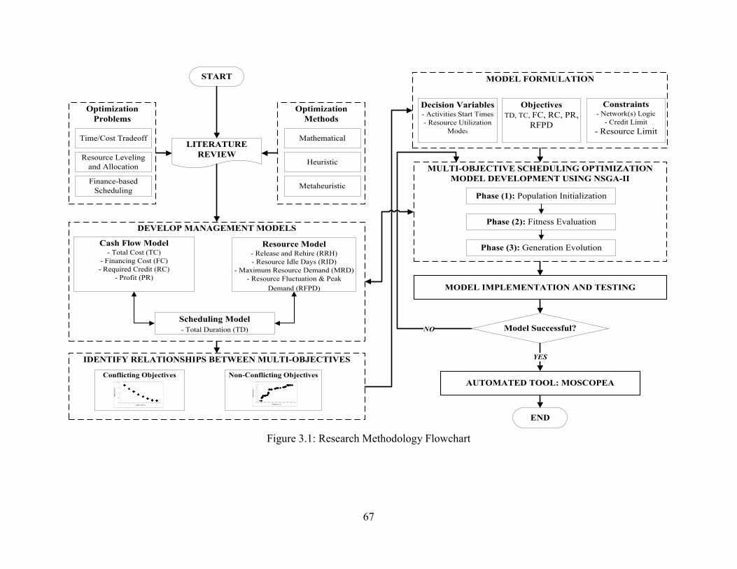
67
START
MODEL IMPLEMENTATION AND TESTING
MULTI-OBJECTIVE SCHEDULING OPTIMIZATION
MODEL DEVELOPMENT USING NSGA-II
Phase (1): Population Initialization
Phase (2): Fitness Evaluation
Phase (3): Generation Evolution
MODEL FORMULATION
Decision Variables- Activities Start Times
- Resource Utilization
Modes
Objectives
TD, TC, FC, RC, PR,
RFPD
Constraints- Network(s) Logic
- Credit Limit
- Resource Limit
Model Successful?
AUTOMATED TOOL: MOSCOPEA
END
DEVELOP MANAGEMENT MODELS
Cash Flow Model- Total Cost (TC)
- Financing Cost (FC)
- Required Credit (RC)
- Profit (PR)
Resource Model- Release and Rehire (RRH)
- Resource Idle Days (RID)
- Maximum Resource Demand (MRD)
- Resource Fluctuation & Peak
Demand (RFPD)
Scheduling Model
- Total Duration (TD)
IDENTIFY RELATIONSHIPS BETWEEN MULTI-OBJECTIVES
Conflicting Objectives
9000
10000
11000
12000
13000
48 49 50 51 52 53 54 55 56 57
OB
JEC
TIV
E (
2)
OBJECTIVE (1)
Non-Conflicting Objectives
750
800
850
900
950
1000
1050
1100
1150
1200
1250
2000 2200 2400 2600 2800 3000 3200 3400 3600 3800 4000
OB
JE
CT
IVE
(2
)
OBJECTIVE (1)
LITERATURE
REVIEW
Optimization
Problems
Finance-based
Scheduling
Resource Leveling
and Allocation
Time/Cost Tradeoff
Optimization
Methods
Metaheuristic
Heuristic
Mathematical
YES
NO
Figure 3.1: Research Methodology Flowchart
68
3.2 DEVELOP MANAGEMENT MODELS
As mentioned earlier, the main objective of this research is to develop a multi-objective
scheduling optimization model for multiple construction projects. The multi-objectives to
be optimized are the: total duration (TD), total cost (TC), financing cost (FC), required
credit (RC), profit (PR), and resource fluctuation and peak demand (RFPD). Thus, three
management models are developed to determine such objectives’ values as follows:
1. Scheduling Model: to determine the TD
2. Cash Flow Model: to determine the TC, FC, RC, and PR
3. Resource Model: to determine the RFPD
Cash flow and resource models, which are presented in Chapter 2, only fit single project.
As a result, since this study focuses on multiple projects; the cash flow and resource
models described in the literature review are modified in order to suit and consider the
existence of more than one project. Beside determining the TD, the scheduling model
acts as the main core of the three management models as it is linked to both the cash flow
and resource models to determine their respective objectives. In other words, both cash
flow and resource models depend on the schedule obtained from the scheduling model.
3.2.1 Multiple Projects Cash Flow Model
Let direct cost disbursements of all activities performed on day i for project z be denoted
as (ci)z, this is referred to as direct cost disbursement of day i for project z. Thus (ci)z can
be calculated as follows:
(𝑐𝑖)𝑧 = ∑ (𝑐𝑣𝑚𝑖)𝑧𝑛𝑖𝑣=1 i = 1 ,2 ,…..Dz ……………..………..…………………(3.1)

69
Where; ni = number of activities ongoing with day i; (cvmi)z = direct cost disbursement
rate of activity v using resource utilization mode m in day i for project z; and Dz = total
project duration of project z.
The cash outflow during a typical period t - a week in this model – for project z is
represented by (Et)z and encompasses the costs of overheads and taxes in addition to the
direct cost disbursements including the costs of materials, equipment, labor, and
subcontractors. (Et)z can be calculated as follows:
(𝐸𝑡)𝑧 = ∑ (𝑐𝑖)𝑧𝑑𝑖=1 + (𝑂𝑡)𝑧 ……………….………………………….…………….…(3.2)
Where; d = number of days comprising a week; and (Ot)z = expenses of overheads, taxes,
mobilization, and bond at period t for project z.
As a result, in case of multiple simultaneous projects, the cash outflow at the end of a
given period includes the Et components of the individual projects ongoing during the
same week. Et can be calculated as follows:
𝐸𝑡 = ∑ (𝐸𝑡)𝑧𝑍𝑧=1 ……………….…………………….……………….…………..……(3.3)
Where; Z = total number of projects.

70
On the other hand, the cash inflow for project z, represented by (Pt)z, includes the
payments contractors receive, at the ends of periods, as an earned value of the
accomplished works calculated based on the unit prices. (Et)z can be calculated as
follows:
(Pt)z = Kz(Et)z……………………………………………………………….…….……(3.4)
Where; Kz = multiplier for project z to determine the amount of payment for a given
amount of disbursement (Et)z (Kz > 1). In order to calculate the multiplier Kz; first a bid
price factor BFz for project z must be calculated as follows:
𝐵𝐹𝑧 =𝑇𝑜𝑡𝑎𝑙 𝑃𝑟𝑖𝑐𝑒𝑧
𝑇𝑜𝑡𝑎𝑙 𝐷𝑖𝑟𝑒𝑐𝑡 𝐶𝑜𝑠𝑡𝑧…………………………………………………………………(3.5)
Then, the amount of retention Rz for project z must be defined. Retention is a percentage
of each bill which clients often withhold to ensure the contractor completes the
construction project satisfactorily. The retained portion of the progress payments will
often be released when the job is completed. In addition, in the case where the contractor
receives from the client an advance payment APz at the beginning of the project; this
amount of advance payment will be cut as a percentage from each bill. As a result the
multiplier Kz can be calculated as follows:
Kz = (1 – (Rz% + APz%)) x BFz ...…………..………….………………………..…….(3.6)

71
It should be noted that the last payment (PT)z will be calculated as shown in Equation 3.4
with adding to the equation the total amount of retention to be as follows:
(PT)z = Kz(Et)z + Rz ……………………………………………………..………...…...(3.7)
In case of multiple simultaneous projects, the cash inflow at the end of a given period
includes the Pt components collected of the projects at this time. Pt can be calculated as
follows:
𝑃𝑡 = ∑ (𝑃𝑡)𝑧𝑍𝑧=1 ……………….…………………………………………….……...…(3.8)
To that point, the total value of the Et and Pt for all the ongoing projects can be
calculated. The rest of the financial parameters described in the literature review are to be
calculated based on Equations 2.11 – 2.18 in Chapter 2.
3.2.2 Multiple Projects Resource Model
Let the total resource demand of all activities performed on day i for project z be denoted
by (ri)z, this is referred to as total resource demand of day i for project z. Thus (ri)z can be
calculated as follows:
(𝑟𝑖)𝑧 = ∑ (𝑟𝑣𝑖)𝑧𝑛𝑖𝑣=1 i = 1 ,2 ,…..Dz …..…..…………………..…………….…(3.9)
Where; ni = number of activities ongoing with day i; (rvi)z = resource demand of activity v
in day i for project z; and Dz = total project duration of project z.

72
As a result the total daily resource demand for all ongoing projects ri can be calculated as
follows:
𝑟𝑖 = ∑ (𝑟𝑖)𝑧𝑍𝑧=1 ……………….…….………………….…………….…………….…(3.10)
Finally, the rest of the resource leveling model parameters described in the literature
review are to be calculated based on Equations 2.1 – 2.4 in Chapter 2.
3.2.3 Multiple Projects Scheduling Model
The main purpose of this model is to develop optimal/near optimal schedules for
construction projects. The model starts by calculating the start times and finish times of
the project activities as shown in Equations 3.11 and 3.12, respectively. The start time is
defined as the earliest start time of activity v when resource utilization mode mv is used.
Similarly, the finish time is defined as the earliest finish time of activity v using resource
utilization mode mv. Accordingly, the total project duration can be calculated as shown in
Equation 3.13.
(stv)z ≥ max:(ftp ,mp)z ……………………………….…………………..…….……....(3.11)
(ftv , mv)z = (stv)z + (dv , mv)z ……………………….…..…………………………….(3.12)
Dz = max:(ftv , mv)z …………………………..……………………..………………..(3.13)

73
Where; (stv)z = start time of activity v in project z; (ftv , mv)z = finish time of activity v
using resource utilization mode mv in project z; (ftp ,mp)z = finish time of activities
preceding activity v using resource utilization mode mp in project z; (dv , mv)z = duration
of activity v when resource utilization mode mv is used in project z; and Dz = total
duration of project z.
3.3 IDENTIFY RELATIONSHIPS BETWEEN MULTI-OBJECTIVES
Multi-objective scheduling optimization of contractors carrying out simultaneous projects
incorporates minimizing duration of group of projects, total cost, financing cost,
maximum required credit, and resource fluctuation and peak demand while maximizing
the profit. In fact, it is impractical to optimize all those objectives simultaneously as some
of them could be non-conflicting.
Identifying the non-conflicting objectives varies from project to another. For instance, in
some projects, both financing cost and total cost can be considered as non-conflicting
objectives where the former represents a percentage of the latter. In other projects,
financing cost depends on the overdraft which depends on many additional factors such
as available cash, subcontracting, and front end loading which can conflict with the total
cost. Also, shortening the project duration to a certain point will reduce the additional
overheads which in turn maximize the profit. However, any further reduction in the
project duration will significantly increase the direct cost and accordingly reduce profit
due to an increase in acceleration costs such as overtime and nighttime shifts.
74
Based on that, the objectives’ set of “total cost and financing cost” and “total duration
and profit” can sometimes in specific cases be non-conflicting objectives. Moreover, both
financing cost and total cost can be added and combined as one objective for more
practicality and simplicity in the optimization process. As a result, the efforts of
contractors should be focused on optimizing the four objectives of combined total cost
and financing cost, required credit, profit, and resource fluctuation and peak demand.
According to a previous study in finance-based scheduling optimization carried by Abido
and Elazouni 2011; the relations among different objectives were illustrated as follows:
First, reducing the financing costs definitely increases the profit and usually takes place
when the project duration is shortened due to the eliminated extra overheads and
liquidated damages. Shortening the project duration requires the continuous utilization of
the available resources during each period which in turn increases the maximum required
credit. Second, minimizing the maximum required credit increases the possibility of the
required credit to be approved by bankers and offers the contractors more leverage to
negotiate better interest rates and terms of payment back but definitely results in an
inevitable increase in the duration and financing costs which in turns decreases the profit.
Third, shortening the duration increases the profit by reducing the overhead costs and the
financing costs but requires high credit, in other words it increases the maximum required
credit.
Since the previous studies did not take into consideration the objective of resource
fluctuation; two experiments are carried to investigate the effect of minimizing the
resource fluctuations and peak demand on the financing cost, required credit, and profit.

75
In these two experiments the two new metrics of resource leveling (RRH and RID)
discussed before are used to measure the resource fluctuations.
Experiment (1): Six-Activity Network:
The first experiment is applied on an example of a six-activity project network that was
presented in El-Rayes and Jun (2009) study as shown in Figure 2.6. In this example, the
minimum reached RRH = 6 and the minimum reached RID = 32. It should be noted that
reaching the minimum RID did not change the initial schedule which can be considered
as an exception since the network is small. The experiment is carried first by reasonably
assuming different direct costs to the project activities and other time, financial, and
contractual data concerning the project as shown in Tables 3.1 and 3.2. Then the cash
flow model that was explained earlier is applied twice; once on the initial schedule and
the other on the minimum RRH schedule to determine for each schedule the financing
cost, maximum required credit, and profit.
Table 3.1: Direct Costs (Experiment 1)
Activity Duration Direct Cost / day Total Direct Cost
A 2 1800 3600
B 2 1400 2800
C 5 2600 13000
D 5 2000 10000
E 5 2500 12500
F 2 2400 4800
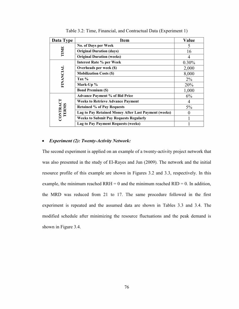
76
Table 3.2: Time, Financial, and Contractual Data (Experiment 1)
Data Type Item Value
TIM
E No. of Days per Week 5
Original Duration (days) 16 Original Duration (weeks) 4
FIN
AN
CIA
L
Interest Rate % per Week 0.30% Overheads per week ($) 2,000 Mobilization Costs ($) 8,000 Tax % 2% Mark-Up % 20% Bond Premium ($) 1,000
CO
NT
RA
CT
TE
RM
S
Advance Payment % of Bid Price 6% Weeks to Retrieve Advance Payment 4 Retained % of Pay Requests 5% Lag to Pay Retained Money After Last Payment (weeks) 0 Weeks to Submit Pay Requests Regularly 1 Lag to Pay Payment Requests (weeks) 1
Experiment (2): Twenty-Activity Network:
The second experiment is applied on an example of a twenty-activity project network that
was also presented in the study of El-Rayes and Jun (2009). The network and the initial
resource profile of this example are shown in Figures 3.2 and 3.3, respectively. In this
example, the minimum reached RRH = 0 and the minimum reached RID = 0. In addition,
the MRD was reduced from 21 to 17. The same procedure followed in the first
experiment is repeated and the assumed data are shown in Tables 3.3 and 3.4. The
modified schedule after minimizing the resource fluctuations and the peak demand is
shown in Figure 3.4.
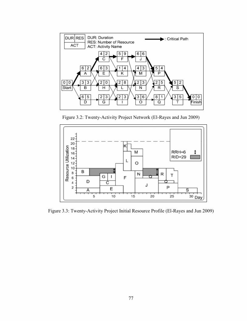
77
Figure 3.2: Twenty-Activity Project Network (El-Rayes and Jun 2009)
Figure 3.3: Twenty-Activity Project Initial Resource Profile (El-Rayes and Jun 2009)

78
Table 3.3: Direct Costs (Experiment 2)
Activity Duration Direct Cost / day Total Direct Cost
A 6 1200 7200
B 3 1400 4200
C 4 1500 6000
D 6 1700 10200
E 6 1800 10800
F 5 2600 13000
G 2 1700 3400
H 2 1400 2800
I 2 1800 3600
J 6 2400 14400
K 1 2200 2200
L 2 2400 4800
M 4 2100 8400
N 2 2200 4400
O 3 2500 7500
P 5 1800 9000
Q 8 1800 14400
R 2 2000 4000
S 5 1400 7000
T 3 1900 5700
Table 3.4: Time, Financial, and Contractual Data (Experiment 2)
Data Type Item Value
TIM
E No. of Days per Week 5
Original Duration (days) 31 Original Duration (weeks) 7
FIN
AN
CIA
L
Interest Rate % per Week 0.30% Overheads per week ($) 3,500 Mobilization Costs ($) 25,000 Tax % 2% Mark-Up % 20% Bond Premium ($) 2,500
CO
NT
RA
CT
TE
RM
S
Advance Payment % of Bid Price 6% Weeks to Retrieve Advance Payment 7 Retained % of Pay Requests 5% Lag to Pay Retained Money After Last Payment (weeks) 0 Weeks to Submit Pay Requests Regularly 1 Lag to Pay Payment Requests (weeks) 1

79
Figure 3.4: Twenty-Activity Project Minimum Resource Profile (El-Rayes and Jun 2009)
Results:
The results obtained from the two experiments - as shown in Table 3.5 - indicate that as
the RRH or RID are minimized along with the MRD, the maximum required credit
increases. This is for a reason that better and efficient utilization of resources reduces the
resource idle days which in turn leads to continuous use of resources in each period
resulting to an increase in the required credit. Simultaneously, minimizing resource
fluctuations results in an increase in the financing cost which eventually decreases the
profit. However, this case may be the opposite if the optimization model in hand will
consider the resource idle days cost. In other words, minimizing resource fluctuations can
increase the financing cost but at the same time reduces the resource idle days cost which
can positively affect the profit. Therefore, the objectives of duration, financing costs,

80
maximum required credit, profit, and resource fluctuations and peak demand will
constitute a set of multiple contractor conflicting objectives.
Table 3.5: Effect of Minimizing Resource Fluctuations
OBJECTIVES
SCHEDULE
EXPERIMENT (1) EXPERIMENT (2)
Financing
Cost
Required
Credit Profit
Financing
Cost
Required
Credit Profit
Initial
Schedule 255 41,262 12,514 732 39,104 38,477
Minimum Resource
Fluctuation Schedule 277 43,901 12,492 774 42,690 38,435
3.4 MULTI-OBJECTIVE OPTIMIZATION MODEL FORMULATION
The principles of multi-objective optimization are different from that of a single objective
optimization. The main goal in a single objective optimization is to find the global
optimal solution, resulting in the optimal value for the single objective function. In a
multi-objective optimization problem, it is aimed to simultaneously optimize several
objective functions. Generally, these functions are non-commensurable and often
represent competing and conflicting objectives. Multi-objective optimization with such
conflicting objectives gives rise to a set of optimal solutions, instead of one optimal
solution. The reason for the optimality of many solutions is that no one is better than any
other one with respect to all objectives. These optimal solutions are referred to as Pareto-
optimal solutions.
The primary purpose of this development stage is to create a robust optimization model
formulation that supports the multi-objective scheduling problem. As shown in Figure

81
3.5, the present model is formulated in two major steps: (1) determining the major
decision variables and (2) formulating the major six objectives of duration, total cost,
financing cost, maximum required credit, profit, and resource fluctuations and peak
demand in a robust optimization model. Although it was discussed in the previous section
that not all of the listed objectives are conflicting, yet, all of them will be formulated.
That is to add flexibility in the model to select the set of objectives to be optimized
simultaneously. In other words, different tradeoffs between different set of selected
objectives can be obtained from the model. The merit of this flexibility is to allow the
contractor to examine the impact of one or more objectives over the other on the projects’
schedule. The selection of such objectives is based on whether they are conflicting or not
as well as the contractor’s preference.
3.4.1 Decision Variables
For each construction activity in the project, the present model is designed to consider
two decision variables that may have an impact on the selected conflicting objectives.
The first decision variable comprises the start times (st) of each activity in a project. The
second decision variable – since the study focuses on multimode activities - will include
different daily crew formations which represent feasible sizes and configurations for
construction crews. This variable will be called resource utilization mode (m) of which
each has a different activity duration and cost. The major challenge confronting
construction planners in this problem is to select an optimal start time and a resource
utilization mode from the available set of feasible alternatives for each activity in the
project. The possible combinations of these alternatives create a large search space,

82
where each solution in this space represents a possible start time and resource utilization
mode for delivering the project. As a result the optimization model to be built will help
planners in the challenging task of searching this large solution space in order to identify
optimal/near optimal start time of activities and their resource utilization mode that
achieves multiple project objectives.
3.4.2 Optimization Objectives
The multi-objective optimization problem in hand will involve minimizing the duration
of group of projects, total cost, financing cost, maximum required credit, and resource
fluctuation and peak demand while maximizing the profit. The model is designed to
quantify and measure the impact of various activities’ start times and their corresponding
resource utilization mode on the multiple project objectives. Those objectives can be
expressed mathematically as follows:
Objective (1): Minimize Total Project Duration:
O1(TD) = Dz ……...………………………………………………………………….(3.14)
Objective (2): Minimize Total Cost:
𝑂2(𝑇𝐶) = ∑ (𝐸𝑡)𝑇𝑡=1 ………………………………………………………………….(3.15)

83
Objective (3): Minimize Financing Cost:
𝑂3(𝐹𝐶) = ∑ (𝐼𝑡)𝑇𝑡=1 ………………………………………………………….……….(3.16)
Objective (4): Minimize Maximum Required Credit:
𝑂4(𝑅𝐶) = −𝐹, 𝐹 = 𝑚𝑖𝑛{𝐹𝑡′: 𝑡 = 1,2, … , 𝑇}………...…………………….……….(3.17)
Objective (5): Minimize Resource Fluctuations and Peak Demand:
𝑂5(𝑅𝐹𝑃𝐷) = (𝑊1𝑥𝑅𝑅𝐻) + (𝑊2𝑥𝑀𝑅𝐷)………...………………………..……….(3.18a)
OR
𝑂5(𝑅𝐹𝑃𝐷) = (𝑊1𝑥𝑅𝐼𝐷) + (𝑊2𝑥𝑀𝑅𝐷)………...………………………..….…….(3.18b)
Objective (6): Maximize Profit:
𝑂6(𝑃𝑅) = 𝑁′𝑇………...……………………………………………………..……….(3.19)

84
DECISION VARIABLES
st1 st2 ….. stv ….. stV m1 m2 ….. mv ….. mV
st1 st2 ….. stv ….. stV m1 m2 ….. mv ….. mV
Solution (1)
Solution (N)
Start Times Resource Utilization Modes
OPTIMIZATION OBJECTIVES
Minimize Resource Fluctuations
and Peak DemandMinimize Total Duration
Minimize Total Cost
Minimize Maximum Required
CreditMinimize Financing Cost
Maximize Profit
Figure 3.5: Decision Variables and Optimization Objectives
Where; W1 = planner defined weight or relative importance for the RRH or RID; and W2
= planner defined weight or relative importance for the MRD. Construction planners can
specify these weights of W1 and W2 to reflect the relative importance of minimizing
undesirable resource fluctuations and minimizing the MRD in their projects. The relative

85
importance of these two important objectives depends on the specific project conditions
and needs and may vary from one project to another. Accordingly, the present model is
designed to provide construction planners with the flexibility to easily experiment with
varying weights and analyze their impact on the generated optimal schedules.
Although the “profit” objective is dependent on the “total cost” and “financing cost”
objectives, yet such objectives are formulated separately to give more flexibility in
solving the desired scheduling optimization problem. In other words, the optimization
model can be used to solve separately time/cost tradeoff, resource leveling, resource
allocation, or finance-based scheduling problems. Alternatively, integration of such
problems can be also solved. Time/cost tradeoff problem is applied when the contractor’s
first concern is to identify the optimal/near optimal execution mode for each activity. In
such case, the selected objectives to optimized simultaneously will be the total duration
and total cost. Resource leveling is applied when the contractor’s first concern is to
search for an optimal schedule that minimizes the project’s undesired resource fluctuation
within the required duration. In this case the selected objective to be optimized will be the
RRH or RID resource leveling metric. Resource allocation is applied when resources are
limited and an optimal/near optimal schedule is required such that the resource limit is
not exceeded with the minimum extension in duration (if required). In this case, the
selected objectives to be optimized simultaneously will the total duration and MRD.
Finance-based scheduling problem is applied when maximum required credit is needed to
be generally minimized or minimized below a certain credit limit while maximizing the
contractor’s profit. In this case, the selected objectives to be optimized simultaneously

86
will be the maximum required credit and the maximum profit. Combinations of such
problems can also be achieved depending on the project’s main objective. For example,
both resource leveling and allocation can be solved simultaneously by selecting the
RFPD objective. Also, finance-based scheduling can be integrated with both resource
leveling and allocation in order to achieve optimal/near optimal schedules that minimizes
the undesirable resource fluctuations and peak demand while maximizing the profit and
keeping the maximum required credit below a specified credit limit.
The optimization problem including the objective function and constraints can be
formulated as shown in Equations 3.20 – 3.25:
Decision Variables
𝑥𝑧 = {(𝑠𝑡, 𝑚)1, (𝑠𝑡, 𝑚)2, … . , (𝑠𝑡, 𝑚)𝑣, … , (𝑠𝑡, 𝑚)𝑁𝐴𝐶𝑇}, 𝑧 = 1,2, … , 𝑍 ……...….…(3.20)
Where;
𝑋 = {𝑥1, 𝑥2, … . , 𝑥𝑧 , … , 𝑥𝑍} …………………………………..………………………(3.21)
Minimize/Maximize
Oi(X), i = 1,2,…,NOBJ …………….…………………………….…...……...(3.22)

87
Subject to
𝑠𝑡𝑘 − 𝑠𝑡𝑣 − 𝑑𝑚𝑣≥ 0, k ε SCv …………………………………..….(3.23)
RC ≤ CL……..………………………………………...……..………….……(3.24)
MRD ≤ RL……………………………………………………………………(3.25)
Where; Oi = ith objective; Z = total number of projects; xz = vector that represents a
candidate activities’ start times and their associated resource utilization mode for the zth
project; X = matrix that represents candidates’ project schedule and their activities’
associated resource utilization mode for all projects; stv = start time of activity v;
𝑑𝑚𝑣 = duration of activity v based on its associated resource utilization mode; stk = start
times of successors of activity v; mv = resource utilization mode of activity v; NACT =
number of project’s activities; NOBJ = number of objectives; SCv = set of successors of
activity v, CL = credit limit, and RL = resource limit.
For a scheduling problem having multiple objectives, there exist two possibilities of any
two solutions X1 and X2. The first is that one solution dominates the other when it is better
with respect to all the objective values. The second possibility is that no one dominates
the other when none is better than the other with respect to all the objective values. In the
current minimization problem, a schedule X1 dominates X2 if the condition shown in
Equation 3.26 is met as follows:

88
Decision Variables:
- Activities’ Start Time (st)
- Activities’ Resource Utilization Mode (m)
Objective Functions:
- Minimize Total Duration (TD)
- Minimize Total Cost (TC)
- Minimize Financing Cost (FC)
- Minimize Required Credit (RC)
- Minimize Resource Fluctuation & Peak Demand (RFPD)
- Maximize Profit (PR)
Subject to:
- Precedence Relationships
- Credit Limit
- Resource Limit
- st , m > 0
i ε{1,2,…,NOBJ}: Oi(X1) ≤ Oi(X2) ………………..………………...………...……(3.26)
Dominance of X1 can be alternately written as: X2 is dominated by X1. The violation of
the condition stated in Equation 3.26 implies that X1 does not dominate X2 as shown in
Equation 3.27.
i ε{1,2,…,NOBJ}: Oi(X1) ≤ Oi(X2) …………..……………………………….….…(3.27)
Generally, the multi-objective optimization algorithm must guide the search toward the
Pareto-optimal region, and maintain population diversity in the Pareto-optimal front. The
first task is a common goal in all optimization algorithms. The second task is unique to
multi-objective optimization. A summary of the full model formulation is shown in
Figure 3.6.
Figure 3.6: Model Formulation Summary

89
3.5 MULTI-OBJECTIVE OPTIMIZATION MODEL DEVELOPMENT
As mentioned earlier in Chapter 2, both mathematical and heuristic approaches were
found to be inefficient and inflexible when solving practical construction scheduling
optimization problems. This led to focusing on using metaheuristic techniques in solving
multi-objective construction scheduling optimization problems. Among the different
metaheuristics, NSGA-II is selected in this research as it stands out for its fast non-
dominated sorting approach, elitism approach, and its overall capability to maintain a
better solution spread.
This step of research methodology involves the development of the multi-objective
scheduling optimization model using NSGA-II to optimize the mentioned objectives
without violating the set constraints. The designed model performs genetic algorithms
operations in three main phases: (1) population initialization phase that generates an
initial set of N possible solutions for the problem; (2) fitness evaluation phase that
calculates the mentioned objectives of each generated solution; and (3) generation
evolution phase that seeks to improve the fitness of solutions over successive generations
using the NSGA-II technique. The model is intended to be used in the initial planning
stage for the project(s) being considered for bidding as well as during the construction
phase. Usually, during construction, the project(s) being executed may fall ahead or
behind the planned schedule. Moreover, new project(s) may be considered with the
existing ones. Thus it is very important for the model to accommodate such changes and
additions by updating the planned schedules during the construction phase.

90
The model can be applied to solve the resource leveling, resource allocation, and finance-
based scheduling problems for either single or multiple projects. On the other hand, the
model solves the time/cost tradeoff problem for only single project where each individual
project has its unique time/cost tradeoff. Detailed description of the model development
will be explained later in Chapter 4.
3.6 MODEL IMPLEMENTATION AND TESTING
After developing the multi-objective optimization model, it is tested using different case
studies from literature. The testing is done with respect to three optimization problems:
1. Time/cost tradeoff
2. Resource leveling and allocation
3. Finance-based scheduling
The model testing results are compared with the actual results obtained from literature to
prove its credibility and validity in optimizing such problems. Moreover, the model is
implemented on three other case studies to demonstrate its capabilities in optimizing the
schedules of multiple projects with multi-modes and multi-resources activities. Such
demonstration integrated the problems of finance-based scheduling together with
resource leveling and allocation which is the main scope of this research. The results and
analysis of the model implementation and testing are described in details in Chapter 5.
3.7 AUTOMATED TOOL: MOSCOPEA
Finally, an automated tool named MOSCOPEA, an acronym for Multi-Objective
SCheduling OPtimization using Evolutionary Algorithm, is designed and built to provide
a platform for performing optimization of multiple projects scheduling. The tool is built

91
with a friendly graphical user interface using the C# language. The C# offers the potential
of being available across many platforms. It is a very powerful high-level language, an
object-oriented programming language encompassing imperative, declarative, functional,
generic, and component-oriented programming language. The automated tool detailed
description is presented in Chapter 6.

92
CHAPTER 4: MULTI-OBJECTIVE SCHEDULING OPTIMIZATION
MODEL DEVELOPMENT
This chapter is divided into two main sections. The first section describes the major
features of the optimization model to be developed using the NSGA-II technique. The
second section illustrates the detailed process of developing the multi-objective
scheduling optimization model. Related to financing and resources, there are two model
options: (1) non-constrained credit limit and resource limit; and (2) constrained credit
limit and resource limit. The first option will take into account the constraint of
preserving the precedence relationships between the projects’ activities only. While the
second option will also take into consideration the constraint of preserving precedence
relationships between the projects’ activities in addition to preventing the maximum
required credit and the maximum resource demand from exceeding the specified credit
limit and resource limit, respectively. It should be noted that this optimization takes into
account multiple projects with multimode activities using multi-resources. Generally, the
input of the model as shown in Figure 4.1 includes the initial schedules of the projects
along with their time, financial, and contractual terms. On the other hand, the output will
include different optimized schedules that achieve the desired objectives.
4.1 MODEL BASIC FEATURES
Prior developing the optimization model, there are five basic features to be described,
namely: (1) extension scheme; (2) chromosome structure; (3) chromosome fitness
evaluation; (4) infeasible chromosome treatment; and (5) reproduction.

93
Figure 4.1: Model Overview
4.1.1 Extension Scheme
Minimizing the initial maximum required credit can be achieved by performing several
trials of shifting the projects’ activities within their floats while keeping the original
project’s duration unchanged. However, such minimization may still exceed the
Project 1
Project 2
Project Z
SO
LU
TIO
N 2
….
…
Project 1
Project 2
Project Z
SO
LU
TIO
N 1
….
…
Project 1
Project 2
Project Z
SO
LU
TIO
N N
….
…
OUTPUT
Optimized Schedules
INTPUT
Initial Schedules
Project 1
Project 2
Project Z
NSGA-II
OPTIMIZATION

94
contractor’s credit limit. Thus, the project may be required to be extended beyond its
original duration to achieve the desired credit limit. Although such extension has the
drawbacks of increasing the overheads costs and implying liquidated damages to the
contractor, yet it is essential if the contractor’s financing capability is limited. The basic
concept here is to minimize such extension.
Based on the above, it is essential to devise a project initial scheme and extension
scheme. For instance, the initial scheme for the 5 month schedule shown in Figure 4.2a is
illustrated in Figure 4.2b which is basically a bar chart with total floats portrayed before
activities. The extension scheme, as illustrated in Figure 4.3, is a modification of the
initial scheme that allows a definite extension increment (5 months in Figure 4.3) to the
initial project duration to determine an extended duration, and extends total floats of
activities by the extension increment to produce adjusted total floats. The adjusted total
float is the time space within which an activity can be shifted without affecting the
extended project duration. For instance, Activity (A) can be shifted all the way to the end
of its adjusted total float and still allows us to finish Activity (F), which depends on
Activity (A), before the end of its adjusted total float. Thus, the shift of Activity (A)
could be done without causing further extension beyond the extended project duration.
Practically, numerous extended schedules could be produced for a given schedule. Thus,
a fundamental objective of the method is to minimize schedule extensions. Extension
schemes allow formulating schedules such that negative cash values are always
minimized, and minimize extensions in the initial critical path method schedules. Thus,

95
extension schemes transform the process of seeking extended schedules that fulfill cash
constraints from searching in boundless solution spaces to searching in well-defined and
definite solution spaces (Elazouni and Metwally 2005).
Figure 4.2: Initial Scheme
Figure 4.3: Extension Scheme
2 3 4 5 1
AC
TIV
ITY
MONTH
B
C
D
E
F
A
2 3 4 5 1
AC
TIV
ITY
MONTH
B
C
D
E
F
A
Total Float
Total Float
Total Float
Total Float
(a) (b)
AC
TIV
ITY
MONTH
2 3 4 5 1 7 8 9 10 6
B
C
D
E
F
A
Adjusted Total Float
Adjusted Total Float
Adjusted Total Float
Adjusted Total Float
Adjusted Total Float
Adjusted Total Float

96
4.1.2 Chromosome Structure
The chromosome structure, as shown in Figure 4.4, is to be set as two strings of genes
separated by a heavy line in the middle. The left hand string represents the start times of
the activities. While, the right hand strings represents the resource utilization mode of
activities’ alternatives. As such, each chromosome represents one possible schedule.
Figure 4.4: Chromosome Structure Representation
4.1.3 Chromosome Fitness Evaluation
When a chromosome is being evaluated, its start time values and resource utilization
modes are assigned to the corresponding project activities to produce a new schedule.
Such schedule produced by each chromosome is evaluated based on its resulted
objectives’ values by applying non-dominance ranking. All chromosomes are sorted
based on non-domination into each front. The first front being completely non-dominant
set in the current population and the second front being dominated by the chromosomes
in the first front only and the front goes so on. Each chromosome in the each front are
st1 st2 … stv … stV m1 m
2
… mv … mV
1 2 … v … V 1 2 … v … V
Legend:
X
Activity
Y
Activity Start Time
Legend:
Z
X
Activity
Activity Resource
Utilization Mode
97
assigned a rank (fitness) value based on the front in which they belong to. Chromosomes
in first front are given a fitness value of 1 and chromosomes in second are assigned
fitness value of 2 and so on. In addition to the fitness value, the crowding distance is
calculated for each chromosome as a secondary ranking. As mentioned before, the
crowding distance is a measure of how close a chromosome is to its neighbors. Large
average crowding distance will result in better diversity in the population.
4.1.4 Infeasible Chromosome Treatment
Infeasible solutions may arise when new individual chromosomes are generated for the
initial population and/or when offspring chromosomes are reproduced within the
population using the crossover and mutation operators. The infeasibility takes place by
having a chromosome that either: (1) violates the precedence logical relationship between
the projects’ activities; (2) produces maximum required credit exceeding the set credit
limit; or (3) produces maximum resource demand exceeding the set resource limit.
The first type of infeasibility is treated by improving the crossover and mutation
operators as it will be explained in the next sub-section. As for the second and third type
of infeasibility, the treatment is carried by assigning a lower rank for the infeasible
chromosome throughout the non-domination ranking process. When sorting the entire
population by comparing each two chromosomes at a time, two cases may arise with
respect to infeasibility: (1) one chromosome is feasible while the other is infeasible; and
(2) both chromosomes are infeasible. In the first case, the feasible chromosome is kept in
front X and the infeasible chromosome is shifted to front X+1. Such shifting of the
infeasible chromosome to the next fronts will continue until there is no any feasible

98
chromosome left with it in the same front. The second case happens when all the
infeasible chromosomes in the entire population are shifted to the last front Z. In other
words, front Z will contain all the infeasible chromosomes. In this case, when two
infeasible chromosomes are compared, the chromosome with the lower constraint
violation will be kept in front Z while the other will be further shifted to front Z+1 and so
on. This way of treatment decreases the chances that these infeasible chromosomes are
selected for reproduction in the subsequent generations and eventually exclude them from
the population after some iterations.
4.1.5 Reproduction
The reproduction process among the population members takes place by either crossover
or mutation as explained before. However, the basic crossover or mutation operators may
not maintain the precedence relationship between the activities. Operations facilitated by
crossover and mutation alter the contents of the genes, thus causing the violation of the
precedence constraint. In other words, most new strings generated from crossover and
mutation becomes infeasible solutions. For example, for the bar chart shown in Figure
4.2, it is noticed after the basic crossover that offspring 2 in Figure 4.5 became an
infeasible solution, as Activities (D), (E), and (F) are scheduled to start before the finish
of the preceding activities, violating the constraint of precedence. Consequently, repair of
infeasible chromosomes is required after each crossover or mutation operation which
consumes processing time.
Initially, an improved crossover was used to repair infeasible genes causing prolonged
processing time due to computational inefficiency. To overcome this problem Abido and

99
START
0 00
0 0
FINISH
13 130
13 13
A
5 72
0 2
TF = 5
B
5 83
0 3
TF = 5
C
3 52
0 2
TF = 3
D
0 33
0 3
TF = 0
E
7 103
2 5
TF = 5
F
8 102
3 5
TF = 5
G
5 72
2 4
TF = 3
H
3 63
3 6
TF = 0
I
7 103
4 7
I
TF = 3
J
6 104
6 10
TF = 0
K
10 133
7 10
TF = 3
L
11 132
7 9
TF = 4
M
10 133
10 13
TF = 0
Activity
###
Total Float
Late
Start Duration
Late
Finish
Early
Start
Early
Finish
Elazouni (2010) developed an improved crossover and mutation operators that caused
potential reduction in processing time without affecting results. These operators are
explained as follows being applied on the 13-activity CPM network and its seven-day
extension scheme shown in Figures 4.6 and 4.7, respectively.
Figure 4.5: Example of Illegal Offspring from Crossover
Figure 4.6: CPM Network of a 13-Activity Project
Parent 1
Parent 2
Offspring 1
Offspring 2 (Illegal)
0 0 2
A B C
1 2 1
D E F
2 2 4
A B C
3 4 3
D E F
0 0 2
A B C
3 4 3
D E F
2 2 4
A B C
1 2 1
D E F
Legend:
Y
X
Activity Start
Time
Activity

100
1 2 3 4 5 6 7 8 9 10 11 12 13 14 15 16 17 18 19 20
J'
DAY
H
H'
J
I
I'
D
D'
M
M'
G
G'
L'
C
C'
F
F'
L
E'
K
K'
B
B'
A'
E
A
Figure 4.7: Seven-day Extension of the 13-Activity Project
4.1.5.1 Improved Crossover
The algorithm of the crossover operator comprises two paths: forward path and backward
path. The latter utilizes the conventional forward free float (FFF) while the former
utilizes the backward free float (BFF). The BFF is the number of days the start time of an
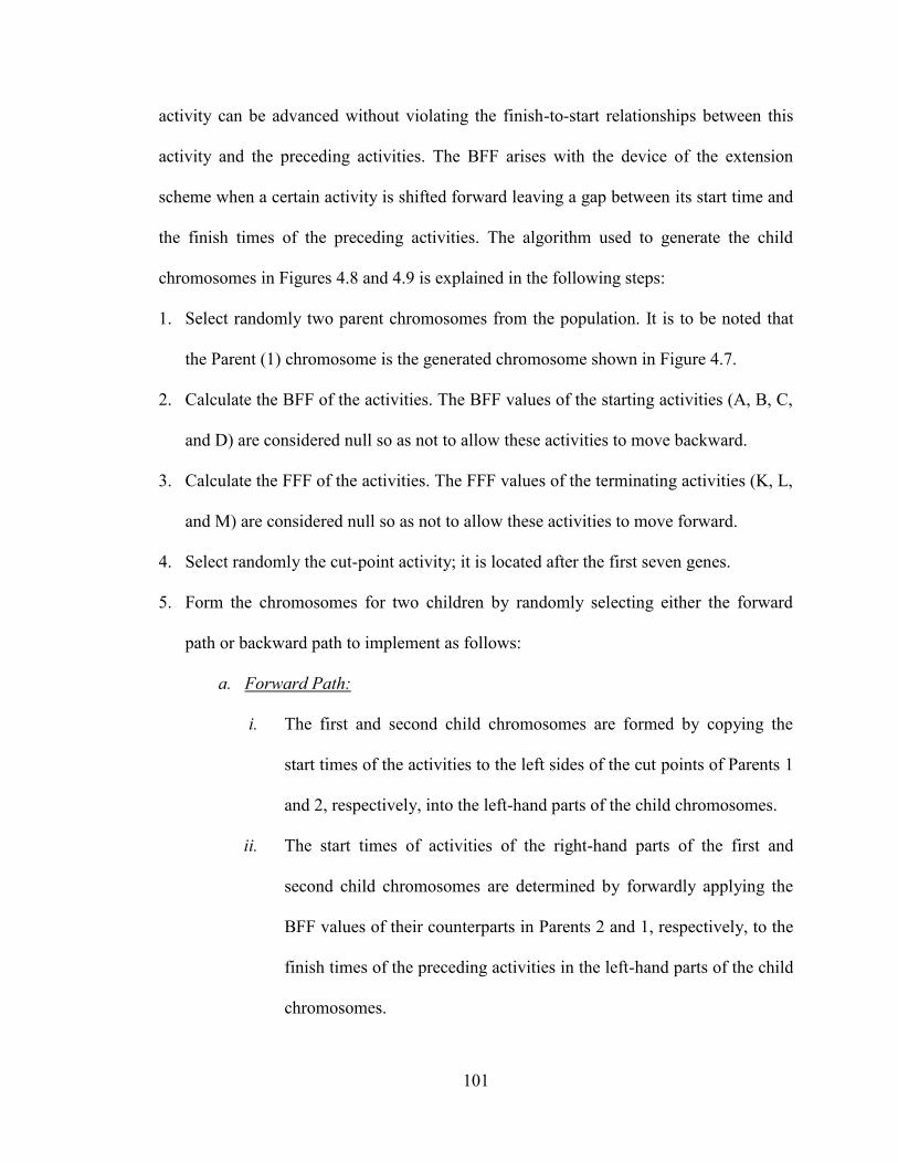
101
activity can be advanced without violating the finish-to-start relationships between this
activity and the preceding activities. The BFF arises with the device of the extension
scheme when a certain activity is shifted forward leaving a gap between its start time and
the finish times of the preceding activities. The algorithm used to generate the child
chromosomes in Figures 4.8 and 4.9 is explained in the following steps:
1. Select randomly two parent chromosomes from the population. It is to be noted that
the Parent (1) chromosome is the generated chromosome shown in Figure 4.7.
2. Calculate the BFF of the activities. The BFF values of the starting activities (A, B, C,
and D) are considered null so as not to allow these activities to move backward.
3. Calculate the FFF of the activities. The FFF values of the terminating activities (K, L,
and M) are considered null so as not to allow these activities to move forward.
4. Select randomly the cut-point activity; it is located after the first seven genes.
5. Form the chromosomes for two children by randomly selecting either the forward
path or backward path to implement as follows:
a. Forward Path:
i. The first and second child chromosomes are formed by copying the
start times of the activities to the left sides of the cut points of Parents 1
and 2, respectively, into the left-hand parts of the child chromosomes.
ii. The start times of activities of the right-hand parts of the first and
second child chromosomes are determined by forwardly applying the
BFF values of their counterparts in Parents 2 and 1, respectively, to the
finish times of the preceding activities in the left-hand parts of the child
chromosomes.

102
iii. The forward path may result in durations of the offspring chromosomes
that exceed the duration of the extension scheme. This happened in
Child 1 as Activity M ends at Day 22. These chromosomes are
considered infeasible.
b. Backward Path:
i. The first and second child chromosomes are formed by copying the start
times of the activities to the right sides of the cut points of Parents 1 and
2, respectively, into the right-hand parts of the child chromosomes.
ii. The finish times of the activities of the left-hand parts of the first and
second child chromosomes are determined by backwardly applying the
FFF values of their counterparts in Parents 2 and 1, respectively, to the
start times of the following activities in the right-hand parts of the child
chromosomes. The start times are determined based on the finish times.
iii. The backward path may result in the negative start time of certain
activities in the beginning on the network. In this case, the start times of
all the activities of the network are increased to make this activity start at
Day 0.
4.1.5.2 Improved Mutation
The improved mutation operator also utilizes the FFF and BFF to change the start time of
the mutated activity. The developed algorithm ensures the feasibility of the schedule after
mutation. The steps of the improved mutation operator are outlined as follows and
illustrated in Figure 4.10:
1. Select randomly one activity, say, Activity E.

103
A B C D E F G H I J K L M
3 5 4 7 6 9 6 10 9 13 13 12 17
A B C D E F G H I J K L M
4 7 6 5 9 13 10 9 14 12 17 17 17
A B C D E F G H I J K L M
0 0 0 0 1 1 0 0 1 0 1 0 0
0 0 0 0 3 3 2 1 2 0 0 0 1
A B C D E F G H I J K L M
3 5 4 7 6 9 6 11 10 14 13 13 19
A B C D E F G H I J K L M
4 7 6 5 9 13 10 8 13 11 17 16 15
Cut Point
Cut Point
Backward Free Floats (BFF)
Activity
Parent 1
Parent 2
Child 1
Child 2
Parent 1
Parent 2
2. Determine the FFF and BFF of the selected activity; for Activity E, the FFF is 4 days
and the BFF is 1 day.
3. Shift randomly the activity forward or backward within the range determined by the
FFF and the BFF; the start of Activity E is shifted by 2 days.
Figure 4.8: Improved Crossover Operator – Forward Path
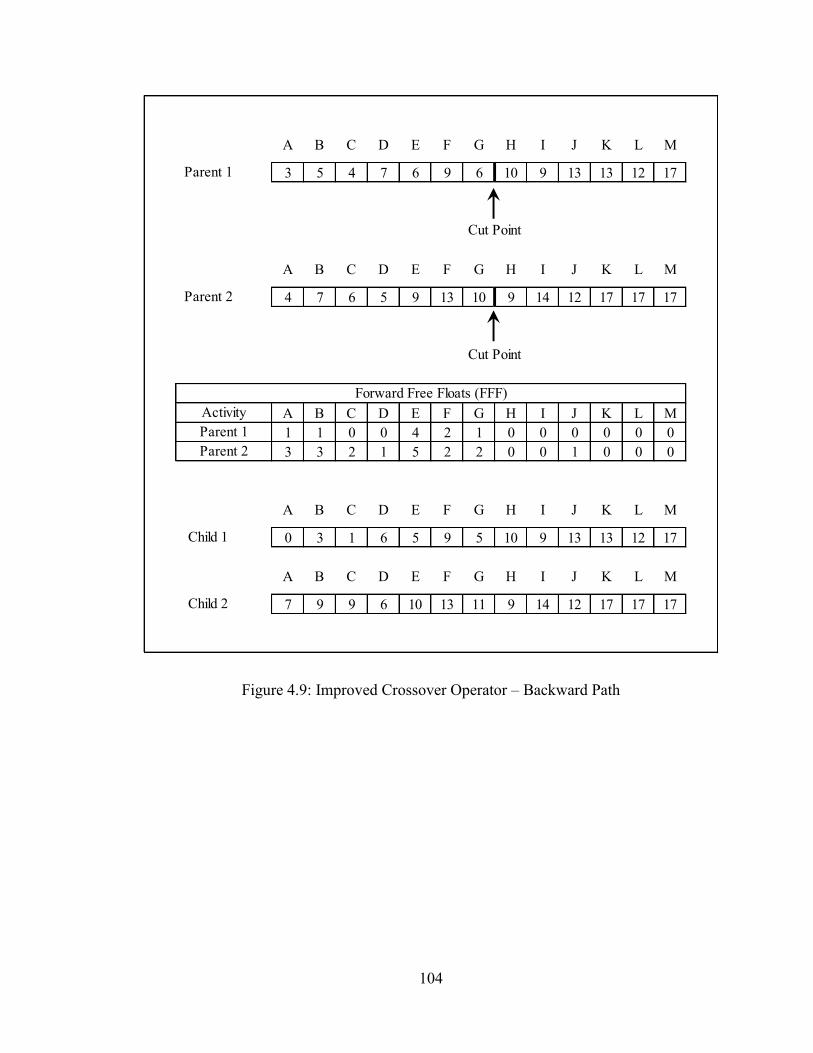
104
A B C D E F G H I J K L M
3 5 4 7 6 9 6 10 9 13 13 12 17
A B C D E F G H I J K L M
4 7 6 5 9 13 10 9 14 12 17 17 17
A B C D E F G H I J K L M
1 1 0 0 4 2 1 0 0 0 0 0 0
3 3 2 1 5 2 2 0 0 1 0 0 0
A B C D E F G H I J K L M
0 3 1 6 5 9 5 10 9 13 13 12 17
A B C D E F G H I J K L M
7 9 9 6 10 13 11 9 14 12 17 17 17
Cut Point
Cut Point
Forward Free Floats (FFF)
Activity
Parent 1
Parent 2
Child 1
Child 2
Parent 1
Parent 2
Figure 4.9: Improved Crossover Operator – Backward Path

105
A B C D E F G H I J K L M
3 5 4 7 6 9 6 10 9 13 13 12 17
A B C D E F G H I J K L M
0 0 0 0 1 1 0 0 1 0 1 0 0
1 1 0 0 4 2 1 0 0 0 0 0 0
A B C D E F G H I J K L M
3 5 4 7 8 9 6 10 9 13 13 12 17
Backward
Forward
Child
Selected Gene
Parent
Free Floats
Activity
Figure 4.10: Improved Mutation Operator
4.2 MODEL DEVELOPMENT
The optimization model at hand, as shown in Figure 4.11, will be developed in three
major phases: (1) population initialization phase that generates an initial set of N possible
solutions for the problem; (2) fitness evaluation phase that calculates the values of the
desired set of objectives to be optimized simultaneously; and (3) generation evolution
phase that seeks to improve the fitness of solutions over successive generations using the
NSGA-II technique. The detailed computational procedure of these three phases is
explained in the following sub-sections. Moreover, a small illustrative example is solved
manually in Appendix A to show the details of the NSGA-II operations focusing on the
“generation evolution” phase.

106
START
PHASE (1): POPULATION INITIALIZATION
Read project and genetic algorithm parameters
Generate random solutions (s = 1 to N) for parent population P1 of first
generation (g = 1)
PHASE (2): FITNESS FUNCTIONS EVALUATION PHASE (3): GENERATION EVOLUTION
Solution (s = 1)
Calculate the total duration (TD) for solution s in
generation g using the scheduling model
Calculate the total cost (TC), financing cost (FC),
maximum required credit (RC), and profit (PR) for
solution s in generation g using the cash flow model
Last solution N?
Next solution (S = s + 1)
Child Population Qg?
Calculate non-domination rank and crowding
distance for each solution (s = 1 to N) of parent
population Pg
Apply crowded tournament selection to create
mating population Mg
Create child population Qg by applying crossover
operation on mating population Mg
Apply mutation operation on child population Qg
Combine child population Qg and parent population
Pg to form a new combined population Rg of size 2N
Calculate non-domination rank and crowding
distance for each solution (s = 1 to 2N) of the newly
created combined population Rg
Sort the new combined population Rg using fast non-
dominated sorting
Keep the top N solutions from the combined
population Rg to form the parent population Pg+1 of
the next generation
Last generation G?
Next generation (G = g + 1)
END
NO
YES
NO
NO
YES
YES
Resource Leveling
Metric?
Calculate the release
and rehire (RRH),
maximum resource
demand (MRD), and
resource fluctuations
and peak demand
(RFPD) for solution s
in generation g using
the resource model
Calculate the resource
idle days (RID),
maximum resource
demand (MRD), and
resource fluctuations
and peak demand
(RFPD) for solution s
in generation g using
the resource model
RIDRRH
Figure 4.11: Model Development Framework

107
4.2.1 Phase (1): Population Initialization
The main purpose of this phase is to generate an initial set of N possible solutions that
will evolve in subsequent generations to a set of optimal/near optimal solutions. The
initialization phase in this model is performed in two main steps as follows:
1. Read project and genetic algorithm parameters needed to initialize the search
process. The project parameters include the following:
- Number of project activities
- Number of resource utilization mode for each activity
- Activity duration and direct cost for each resource utilization mode
- Precedence relationship between activities
- Interest rate %
- Mark-up %
- …etc.
On the other hand, the genetic algorithm parameters will include the following:
- Population size
- Number of generations
- Crossover probability
- Mutation probability
The string size is determined by the model, considering the total number of
activities in the analyzed project(s) multiplied by two since there are two
decision variables for each activity as explained before. The number of
generations G and population size N are identified based on the selected string
size to improve the quality of the solution. Similarly, the mutation and crossover

108
rates are determined considering the population size and the method of selection
employed by the algorithm.
2. Generate random solutions (s = 1 to N) for the initial population P1 in the first
generation (g = 1). These solutions represent an initial set of activity start times
and their corresponding resource utilization mode. This set of possible solutions is
then evolved in the following two phases in order to generate a set of activity
optimal start times and resource utilization modes to establish an optimal tradeoff
between project total duration, financing costs, maximum negative cumulative
balance, and resource fluctuations and peak demand.
4.2.2 Phase (2): Fitness Evaluation
The main purpose of this phase is to evaluate the project’s desired selected multi-
objectives for each possible solution s in generation g to determine the fitness of the
solution. This fitness determines the likelihood of survival and reproduction of each
solution in following generations. As such, this phase will evaluate the fitness function
for each solution by calculating one or more of the following multi-objectives:
1. The total duration TD(s,g) for solution s in generation g using the scheduling
model.
2. The total cost TC(s,g) for solution s in generation g using the cash flow model.
3. The financing cost FC(s,g) for solution s in generation g using the cash flow
model.
4. The maximum required credit RC(s,g) for solution s in generation g using the
cash flow model.
5. The total profit PR(s,g) for solution s in generation g using the cash flow model.
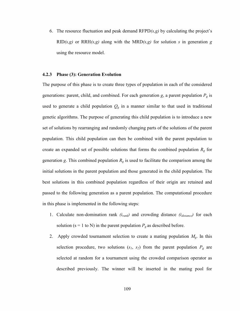
109
6. The resource fluctuation and peak demand RFPD(s,g) by calculating the project’s
RID(s,g) or RRH(s,g) along with the MRD(s,g) for solution s in generation g
using the resource model.
4.2.3 Phase (3): Generation Evolution
The purpose of this phase is to create three types of population in each of the considered
generations: parent, child, and combined. For each generation g, a parent population Pg is
used to generate a child population Qg in a manner similar to that used in traditional
genetic algorithms. The purpose of generating this child population is to introduce a new
set of solutions by rearranging and randomly changing parts of the solutions of the parent
population. This child population can then be combined with the parent population to
create an expanded set of possible solutions that forms the combined population Rg for
generation g. This combined population Rg is used to facilitate the comparison among the
initial solutions in the parent population and those generated in the child population. The
best solutions in this combined population regardless of their origin are retained and
passed to the following generation as a parent population. The computational procedure
in this phase is implemented in the following steps:
1. Calculate non-domination rank (irank) and crowding distance (idistance) for each
solution (s = 1 to N) in the parent population Pg as described before.
2. Apply crowded tournament selection to create a mating population Mg. In this
selection procedure, two solutions (s1, s2) from the parent population Pg are
selected at random for a tournament using the crowded comparison operator as
described previously. The winner will be inserted in the mating pool for

110
reproduction. This selection process is repeated until the mating pool is filled with
N solutions.
3. Create a new child population Qg by applying crossover operation on the solutions
obtained in the mating pool Mg. For each solution in the mating pool the
following steps are performed. The crossover probability (pc) is compared with a
random number in [0, 1] to determine if the crossover operation should be carried
out or not on each solution. If the random number is less than or equal to the
crossover probability then crossover operation is applied on each variable of two
parent solutions selected from the mating pool to produce two offspring solutions.
These two offspring solutions are then stored in the new child population. If the
random number is greater than the crossover probability then the crossover
operation is not carried out and the solution in the mating pool is simply copied
over to the new child population.
4. Apply mutation on the solutions in the new child population Qg. For each variable
in each solution of the new child population the following steps are performed.
The mutation probability (pm) is compared with a random number in [0, 1] to
determine if the mutation operation should be carried out or not on the current
variable. If the random number is less than or equal to the mutation probability
then mutation operation is applied on the variable. The fitness of the generated
child population is then analyzed using the earlier described steps of Phase 2 to
obtain the values of the selected multi-objectives.
5. Combine child population Qg and parent population Pg to form a new combined
population Rg of size 2N. This combined population acts as a vehicle for the

111
elitism, where good solutions of the initial parent population are passed on to the
following generation to avoid the loss of good solutions of the initial parent
population once they are found.
6. Calculate non-domination rank (irank) and crowding distance (idistance) for each
solution (s = 1 to 2N) of the newly created combined population Rg. This step will
perform the same operations as Step 1 of this phase on the new combined
population Rg.
7. Sort the new combined population Rg using the fast non-dominated sorting
procedure. This sorting rule selects solutions with higher non-domination ranks
and breaks ties between solutions with the same rank by favoring solutions with
higher crowding distances.
8. Keep the top N solutions from the combined population Rg to form the parent
population Pg+1 of the next generation. This parent population is then returned to
Step 1 of this phase for generating a new child population as shown in Figure
4.11. This iterative execution of the second and third phases of the model
continues until the specified number of generations is completed.
Due to the unique characteristics of each construction project, the main contribution of
the model developed in this research arises in integrating the issues of both resource
leveling and allocation while considering the contractor’s cash flow for multiple projects.
Such integration enables construction companies in solving simultaneously the problems
of how to prioritize the projects with resource conflicts, how to reasonably allocate the
limited resources among multiple projects to meet the resource requirements of different

112
projects, how to minimize the undesirable resource fluctuations while maximizing the
profit under certain cash limits.

113
CHAPTER 5: IMPLEMENTATION, TESTING, RESULTS AND
ANALYSIS
As previously mentioned, the developed model gives the flexibility of selecting the
objectives required to be optimized simultaneously. Thus, the model can solve
individually the time/cost tradeoff, resource leveling, resource allocation, or finance-
based scheduling problems. Alternatively, integration of such problems can be also
solved. This chapter is divided into two main sections. The first section shows the
implementation of the developed model to test it on three examples retrieved from
literature to solve a time/cost tradeoff problem, integrated time/cost tradeoff and resource
allocation problem, and a finance-based scheduling problem. Consequently, the obtained
results are compared with the previous studies to validate the model. The second section
illustrates the use of the developed model and demonstrates its capabilities by applying it
on three case studies to solve integrated resource leveling, resource allocation, and
finance-based scheduling problems for single and multiple projects.
5.1 MODEL TESTING
Three tests are carried to validate and verify the efficiency of the developed model in
obtaining optimal/near optimal solutions to solve a time/cost tradeoff problem, integrated
time/cost tradeoff and resource allocation problem, and a finance-based scheduling
problem.
114
5.1.1 Test (1): Time/Cost Tradeoff Problem
To test the performance of the developed model in solving time/cost tradeoff problems,
the test example of Feng et al. (1997) is used. The example consists of 18 construction
activities, where each has a number of possible resource utilization modes that can be
used to construct the activity as shown in Table 5.1.
Table 5.1: Data for Test (1) (adapted from Feng et al. 1997)
Activity Predecessor(s)
Mode 1 Mode 2 Mode 3 Mode 4 Mode 5
Du
rati
on
(d
ays)
Cost
($)
Du
rati
on
(d
ays)
Cost
($)
Du
rati
on
(d
ays)
Cost
($)
Du
rati
on
(d
ays)
Cost
($)
Du
rati
on
(d
ays)
Cost
($)
1 - 24 1200 21 1500 16 1900 15 2150 14 2400
2 - 25 1000 23 1500 20 1800 18 2400 15 3000
3 - 33 3200 22 4000 15 4500 - - - -
4 - 20 30000 16 35000 12 45000 - - - -
5 1 30 10000 28 15000 24 17500 22 20000 - -
6 1 24 18000 18 32000 14 40000 - - - -
7 5 18 22000 15 24000 9 30000 - - - -
8 6 24 120 21 208 16 200 15 215 14 220
9 6 25 100 23 150 20 180 18 240 15 300
10 2,6 33 320 22 400 15 450 - - - -
11 7,8 20 300 16 350 12 450 - - - -
12 5,9,10 30 1000 28 1500 24 1750 22 2000 - -
13 3 24 1800 18 3200 14 4000 - - - -
14 4,10 18 2200 15 2400 9 3000 - - - -
15 12 16 3500 12 4500 - - - - - -
16 13,14 30 1000 28 1500 24 1750 22 2000 20 3000
17 11,14,15 24 1800 18 3200 14 4000 - - - -
18 16,17 18 2200 15 2400 9 3000 - - - -
Since this example is a pure time/cost tradeoff problem, the considered decision variable
will be only the resource utilization mode. The objectives selected to be optimized
115
(minimized) will be the “total duration and total cost”. Multiplying the number of
resource utilization modes in each of the 18 activities by each other will result in around
5.9 billion possible combinations for delivering the entire project. Each of these possible
combinations leads to a unique impact on project performance, and the main challenge
here is to search this large search space to find solutions that establish an optimal tradeoff
between construction time and cost.
The developed multi-objective optimization model is used to search this large space of
possible solutions. The model was able to significantly reduce this large space by
precluding dominated solutions in the successive generations of the GA, using the Pareto
optimality principles as explained before. This led to the selection of 31 Pareto optimal
(i.e. non-dominated) solutions for this example as shown in Table 5.2. Each of these
solutions identifies an optimal resource utilization mode for each of the 18 construction
activities and, accordingly, it provides a unique and optimal tradeoff between project time
and cost.
In order to validate the results provided by the current model, they are compared to those
reported in the literature for the same application example (Feng et al. 1997). The
comparison confirms that the current model is capable of generating almost the same set
of optimal solutions as those reported by Feng et al. (1997) for the time/cost tradeoff
problem as shown in Figure 5.1. The figure shows a slight difference between the
obtained solutions of the two models due to the GA’s randomness nature in searching for
optimal/near optimal solutions.

116
Table 5.2: Optimum Solutions for Test (1)
Solution
#
Duration
(days)
Cost
($)
Selected Resource Utilization Mode for Activity #
1 2 3 4 5 6 7 8 9 10 11 12 13 14 15 16 17 18
1 100 133318 5 1 1 1 2 3 1 1 5 3 2 4 1 1 2 1 3 3
2 161 99967 1 1 1 1 1 1 1 5 1 3 1 1 1 1 1 1 1 1
3 106 120318 4 1 1 1 1 2 1 5 5 3 1 4 1 2 2 1 3 3
4 169 99738 1 1 1 1 1 1 1 1 1 1 1 1 1 1 1 1 1 1
5 114 105848 5 2 1 1 1 1 1 3 5 3 1 4 1 1 1 1 3 3
6 101 132316 5 3 2 1 1 3 2 5 5 3 3 4 1 2 2 1 3 3
7 152 100748 1 1 1 1 1 1 1 3 1 3 1 1 1 1 1 1 1 3
8 111 106467 4 1 1 1 1 1 1 5 5 3 3 4 1 2 2 1 3 3
9 105 122262 4 1 1 1 1 2 2 4 5 3 3 4 1 1 2 1 3 3
10 110 107047 5 2 1 1 1 1 1 3 5 3 1 4 1 2 2 1 3 3
11 148 100828 1 1 1 1 1 1 1 3 3 3 1 1 1 1 1 1 1 3
12 145 101167 2 1 1 1 1 1 1 1 5 3 1 1 1 1 1 1 1 3
13 123 104198 2 1 1 1 1 1 1 3 5 3 1 3 1 1 1 1 3 3
14 142 101198 2 1 1 1 1 1 1 3 5 3 1 3 1 1 1 1 1 1
15 127 102898 5 1 1 1 1 1 1 3 5 3 1 3 1 1 1 1 1 3
16 122 104397 5 2 1 1 1 1 1 3 5 3 1 3 1 1 2 1 1 3
17 139 101247 2 1 1 1 1 1 1 3 5 3 1 1 1 1 1 1 1 3
18 138 101967 1 1 1 1 1 1 1 5 5 3 1 1 1 1 2 1 1 3
19 154 100167 1 1 1 1 1 1 1 5 5 3 1 1 1 1 1 1 1 1
20 124 103662 5 2 1 1 1 1 1 4 5 3 1 4 1 1 1 1 1 3
21 120 104567 5 2 1 1 1 1 1 1 5 3 1 4 1 1 2 1 1 3
22 117 105098 5 1 1 1 1 1 1 3 5 3 1 3 1 1 1 1 3 3
23 126 103398 5 2 1 1 1 1 1 3 5 3 1 3 1 1 1 1 1 3
24 132 102167 5 1 1 1 1 1 1 5 5 3 1 1 1 1 1 1 1 3
25 157 100148 1 1 1 1 1 1 1 3 5 3 1 1 1 1 1 1 1 1
26 133 101998 2 1 1 1 1 1 1 3 5 3 1 3 1 1 1 1 1 3
27 104 128261 4 1 1 1 1 3 1 4 5 3 3 4 1 1 2 1 3 3
28 146 100868 1 1 1 1 1 1 1 1 5 3 1 1 1 1 1 1 1 3
29 116 105362 5 1 1 1 1 1 1 4 5 3 1 4 1 1 1 1 3 3
30 102 128467 4 1 1 1 1 3 1 5 5 3 3 4 1 2 2 1 3 3
31 166 99898 1 1 1 1 1 1 1 1 3 2 1 1 1 1 1 1 1 1

117
90000
100000
110000
120000
130000
140000
90 100 110 120 130 140 150 160 170
Co
st (
$)
Duration (days)
(a) Current Model Results
(b) Feng et al. (1997) Results
Figure 5.1: Pareto-optimal Time/Cost Tradeoff Curve for Test (1)

118
5.1.2 Test (2): Integrated Time/Cost Tradeoff and Resource Allocation Problem
The second test is carried using a test example retrieved from Leu and Yang (1999) who
developed a multi-objective GA-based optimization model to perform a time/cost
tradeoff analysis under unconstrained and constrained-resource conditions. The example
consists of nine activities and three resource types required by each activity as shown in
Table 5.3. Each activity has from one to four possible number of resource utilization
modes that can be used to construct the activity. For the resource-constrained condition,
the maximum limit of each resource was assumed to be 10.
Table 5.3: Data for Test (2) (adapted from Leu and Yang 1999)
Activity A B C D E F G H I
Predecessor(s) - A B,D A D,F A F C,E E,G,H
MO
DE
1 Duration (days) 6 9 13 15 14 19 14 8 9
Cost ($) 300 450 600 420 1050 2000 1200 640 560
Resource 1 (crew/day) 3 4 3 5 1 3 3 6 5
Resource 2 (crew/day) 4 5 6 2 5 1 2 3 5
Resource 3 (crew/day) 5 2 5 4 2 1 5 2 5
MO
DE
2 Duration (days) 5 - 12 - 13 18 13 7 -
Cost ($) 480 - 850 - 1450 2600 1900 950 -
Resource 1 (crew/day) 5 - 4 - 1 4 3 6 -
Resource 2 (crew/day) 4 - 6 - 5 2 3 4 -
Resource 3 (crew/day) 5 - 6 - 4 2 6 3 -
MO
DE
3 Duration (days) - - - - 12 17 - - -
Cost ($) - - - - 1860 3220 - - -
Resource 1 (crew/day) - - - - 1 5 - - -
Resource 2 (crew/day) - - - - 5 3 - - -
Resource 3 (crew/day) - - - - 6 3 - - -
MO
DE
4 Duration (days) - - - - - 16 - - -
Cost ($) - - - - - 3860 - - -
Resource 1 (crew/day) - - - - - 6 - - -
Resource 2 (crew/day) - - - - - 4 - - -
Resource 3 (crew/day) - - - - - 4 - - -
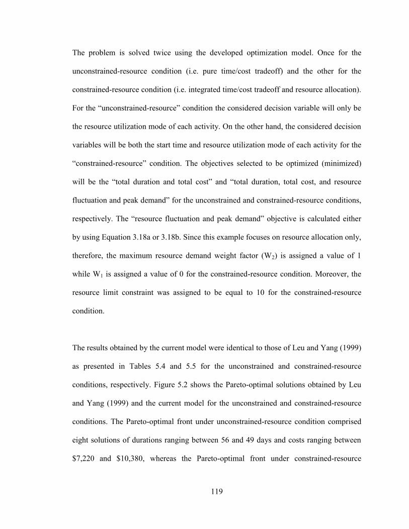
119
The problem is solved twice using the developed optimization model. Once for the
unconstrained-resource condition (i.e. pure time/cost tradeoff) and the other for the
constrained-resource condition (i.e. integrated time/cost tradeoff and resource allocation).
For the “unconstrained-resource” condition the considered decision variable will only be
the resource utilization mode of each activity. On the other hand, the considered decision
variables will be both the start time and resource utilization mode of each activity for the
“constrained-resource” condition. The objectives selected to be optimized (minimized)
will be the “total duration and total cost” and “total duration, total cost, and resource
fluctuation and peak demand” for the unconstrained and constrained-resource conditions,
respectively. The “resource fluctuation and peak demand” objective is calculated either
by using Equation 3.18a or 3.18b. Since this example focuses on resource allocation only,
therefore, the maximum resource demand weight factor (W2) is assigned a value of 1
while W1 is assigned a value of 0 for the constrained-resource condition. Moreover, the
resource limit constraint was assigned to be equal to 10 for the constrained-resource
condition.
The results obtained by the current model were identical to those of Leu and Yang (1999)
as presented in Tables 5.4 and 5.5 for the unconstrained and constrained-resource
conditions, respectively. Figure 5.2 shows the Pareto-optimal solutions obtained by Leu
and Yang (1999) and the current model for the unconstrained and constrained-resource
conditions. The Pareto-optimal front under unconstrained-resource condition comprised
eight solutions of durations ranging between 56 and 49 days and costs ranging between
$7,220 and $10,380, whereas the Pareto-optimal front under constrained-resource

120
conditions comprised five solutions of durations ranging between 65 and 61 days and
costs ranging between $7,220 and $8,960. The comparison of the current model results
against those of Leu and Yang (1999) proves the validity of the current model in solving
scheduling problems of multimode activities using multi-resources.
Table 5.4: Optimum Solutions for Test (2) – Unconstrained Resource
Solution Duration
(days)
Cost ($)
(Current Model)
Cost ($)
(Leu and Yang 1999)
Resource
1
Resource
2
Resource
3
1 49 10,380 10,380 15 13 16
2 50 9,740 9,740 14 13 16
3 51 9,120 9,120 13 13 16
4 52 8,520 8,520 12 13 16
5 53 8,110 8,110 12 13 14
6 54 7,710 7,710 12 13 12
7 55 7,400 7,400 12 13 12
8 56 7,220 7,220 12 13 12
Table 5.5: Optimum Solutions for Test (2) – Constrained Resource
Solution Duration
(days)
Cost ($)
(Current Model)
Cost ($)
(Leu and Yang 1999)
Resource
1
Resource
2
Resource
3
1 61 8,960 8,960 9 8 9
2 62 8,110 8,110 9 7 9
3 63 7,710 7,710 9 7 7
4 64 7,400 7,400 9 7 7
5 65 7,220 7,220 9 7 7
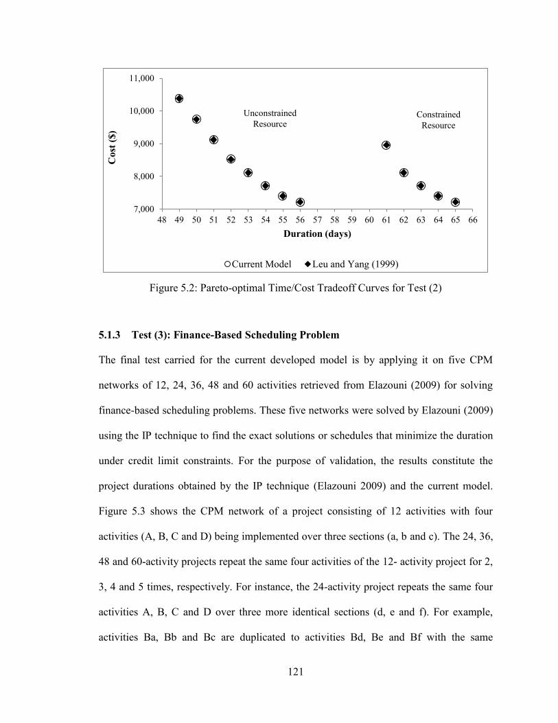
121
Figure 5.2: Pareto-optimal Time/Cost Tradeoff Curves for Test (2)
5.1.3 Test (3): Finance-Based Scheduling Problem
The final test carried for the current developed model is by applying it on five CPM
networks of 12, 24, 36, 48 and 60 activities retrieved from Elazouni (2009) for solving
finance-based scheduling problems. These five networks were solved by Elazouni (2009)
using the IP technique to find the exact solutions or schedules that minimize the duration
under credit limit constraints. For the purpose of validation, the results constitute the
project durations obtained by the IP technique (Elazouni 2009) and the current model.
Figure 5.3 shows the CPM network of a project consisting of 12 activities with four
activities (A, B, C and D) being implemented over three sections (a, b and c). The 24, 36,
48 and 60-activity projects repeat the same four activities of the 12- activity project for 2,
3, 4 and 5 times, respectively. For instance, the 24-activity project repeats the same four
activities A, B, C and D over three more identical sections (d, e and f). For example,
activities Ba, Bb and Bc are duplicated to activities Bd, Be and Bf with the same
7,000
8,000
9,000
10,000
11,000
48 49 50 51 52 53 54 55 56 57 58 59 60 61 62 63 64 65 66
Co
st (
$)
Duration (days)
Current Model Leu and Yang (1999)
Unconstrained
Resource Constrained
Resource
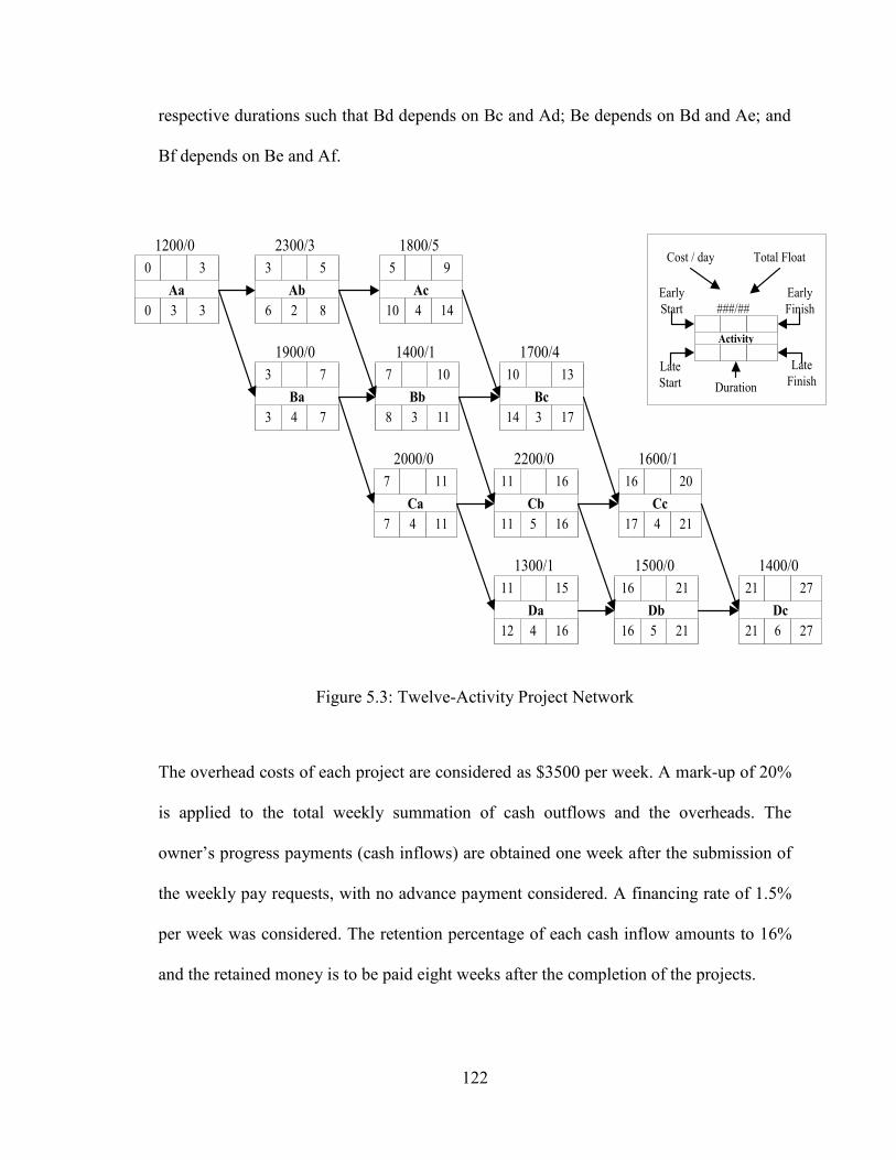
122
Aa
0 33
0 3
1200/0
Ab
6 82
3 5
2300/3
Ac
10 144
5 9
1800/5
Ba
3 74
3 7
1900/0
Bb
8 113
7 10
1400/1
Bc
14 173
10 13
1700/4
Ca
7 114
7 11
2000/0
Cb
11 165
11 16
2200/0
Cc
17 214
16 20
1600/1
Da
12 164
11 15
1300/1
Db
16 215
16 21
1500/0
Dc
21 276
21 27
1400/0
Activity
###/##
Cost / day
Late
Start Duration
Late
Finish
Early
Start
Early
Finish
Total Float
respective durations such that Bd depends on Bc and Ad; Be depends on Bd and Ae; and
Bf depends on Be and Af.
Figure 5.3: Twelve-Activity Project Network
The overhead costs of each project are considered as $3500 per week. A mark-up of 20%
is applied to the total weekly summation of cash outflows and the overheads. The
owner’s progress payments (cash inflows) are obtained one week after the submission of
the weekly pay requests, with no advance payment considered. A financing rate of 1.5%
per week was considered. The retention percentage of each cash inflow amounts to 16%
and the retained money is to be paid eight weeks after the completion of the projects.

123
For each network, three credit limits are set and the main objective is to achieve an
optimal/near optimal schedule that does not exceed such limits. As shown in Table 5.6,
the original maximum required credit for each network is much higher than the set credit
limits. Thus, extension of the project’s original duration for each network may be
sometimes essential in order to achieve the desired credit limits. The main challenge here
is to minimize such extensions.
Table 5.6: Optimum Solutions for Test (3)
Network
Original
Duration
(days)
Original Max.
Required Credit
($)
Credit
Limits
($)
Total Duration
(days) Max. Required
Credit ($)
(Current Model) Elazouni
(2009)
Current
Model
12
Activities 27 50,272.90
40,000 29 29 38,720.74
37,000 32 32 36,602.34
32,000 35 35 31,869.74
24
Activities 42 70,394.90
55,000 43 43 54,050.93
50,000 46 46 49,377.65
43,000 52 52 42,316.50
36
Activities 57 75,238.30
58,000 58 59 57,695.75
54,000 62 62 53,339.99
50,000 66 66 49,659.09
48
Activities 72 77,751.60
58,000 75 75 57,372.61
56,000 77 77 55,813.01
53,000 82 82 52,984.73
60
Activities 87 79,417.23
63,000 87 88 62,591.09
58,000 93 93 57,885.75
57,000 94 94 56,994.29

124
As a result, the objective selected to be optimized (minimized) using the current model
will be the “total duration” under different credit limits constraints. The decision variable
in this example will be the start time of the activities. Table 5.6 indicates clearly that the
results of the current developed model are very comparable to the results of Elazouni
(2009). The difference in the total duration amounted to only one day less in favor of the
IP technique used by Elazouni (2009) in only two cases out of the 15 cases.
5.2 MODEL DEMONSTRATION
The developed optimization model is applied on three case studies to demonstrate its
different optimization capabilities. The first case study is implemented to solve integrated
resource leveling and finance-based scheduling for a small single project. Whereas, the
second and third case studies are implemented to solve integrated resource leveling,
resource allocation, and finance-based scheduling for multiple projects.
5.2.1 Case Study (1): 9-Activity Single Project
The same nine activity single project adopted from Leu and Yang (1999) for the second
test (see section 5.1.2) is used herein as the first case study. The problem was originally
solved as time/cost tradeoff analysis under unconstrained and constrained resource
conditions. However, for demonstration purposes, the problem is to be solved this time
considering financial aspects together with resource aspects. Table 5.7 shows the
financial and contractual data assumed for the original example project to consider the
financial aspects.

125
Table 5.7: Financial and Contractual Data (Case Study 1)
Data Type Item Value
FIN
AN
CIA
L
Interest Rate % per Week 0.80% Overheads % 15% Mobilization Costs % 10% Tax % 2% Mark-Up % 10% Bond Premium % 1%
CO
NT
RA
CT
TE
RM
S
Advance Payment % of Bid Price 5% Weeks to Retrieve Advance Payment a
Retained % of Pay Requests 5% Lag to Pay Retained Money After Last Payment (weeks) 0 Weeks to Submit Pay Requests Regularly 1 Lag to Pay Payment Requests (weeks) 1
a Number of weeks encompassing the total project duration
Unlike the traditional tradeoff problems in the literature, which exclusively consider the
selection of the activities’ execution or resource utilization modes, the current application
considers the specification of the activities start times as well as the selection of
activities’ execution modes as the two main decision variables. Resource leveling is only
considered in this case study by using the resource idle days (RID) leveling metric. Thus,
the “resource fluctuation and peak demand” objective will be determined using Equation
3.18b. However, the RID weight factor (W1) will be assigned a value of 1 while the MRD
weight factor (W2) will be assigned a value of 0. In other words, objective number 5
presented in the model formulation section in Chapter 3 (section 3.4.2) can be entitled as
RID for this case study. Accordingly, the available objectives to be optimized for this
case study will be as follows:
- Total Duration (TD)
- Total Cost (TC)
- Financing Cost (FC)
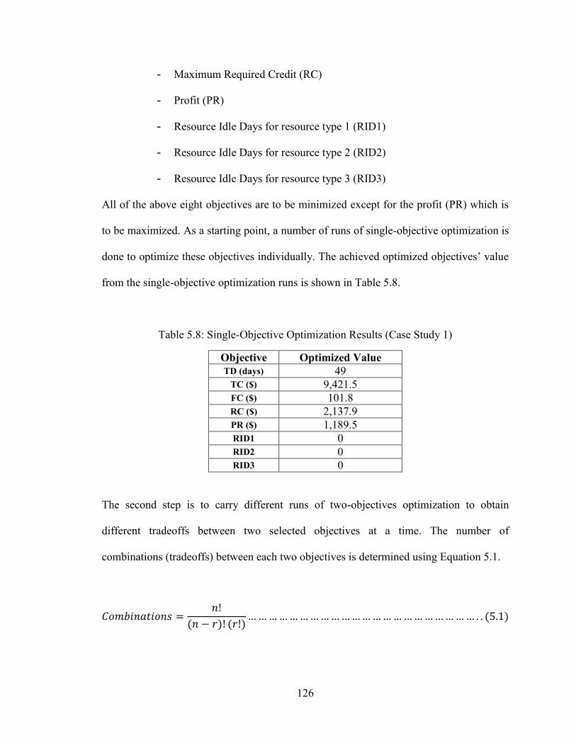
126
- Maximum Required Credit (RC)
- Profit (PR)
- Resource Idle Days for resource type 1 (RID1)
- Resource Idle Days for resource type 2 (RID2)
- Resource Idle Days for resource type 3 (RID3)
All of the above eight objectives are to be minimized except for the profit (PR) which is
to be maximized. As a starting point, a number of runs of single-objective optimization is
done to optimize these objectives individually. The achieved optimized objectives’ value
from the single-objective optimization runs is shown in Table 5.8.
Table 5.8: Single-Objective Optimization Results (Case Study 1)
Objective Optimized Value
TD (days) 49
TC ($) 9,421.5
FC ($) 101.8
RC ($) 2,137.9
PR ($) 1,189.5
RID1 0
RID2 0
RID3 0
The second step is to carry different runs of two-objectives optimization to obtain
different tradeoffs between two selected objectives at a time. The number of
combinations (tradeoffs) between each two objectives is determined using Equation 5.1.
𝐶𝑜𝑚𝑏𝑖𝑛𝑎𝑡𝑖𝑜𝑛𝑠 =𝑛!
(𝑛 − 𝑟)! (𝑟!)… … … … … … … … … … … … … … … … … … … … … … . . (5.1)
127
Where, n = total number of objectives; and r = number of selected objectives. Based on
that, 28 different tradeoffs (combinations) can be obtained considering having a total
number of eight objectives (n) and two objectives to be selected at a time (r).
The main benefit of this step is to identify the relationship between each two objectives
set. Each relationship identifies if the two selected objectives are conflicting or not. It is
actually impractical to consider all of the listed eight objectives to be optimized
simultaneously. Such identification allows the selection of the required objectives to be
optimized simultaneously. Another benefit can be for the contractor in which he/she can
examine the effect of one objective over the other on the project performance. The
current developed model has the flexibility to select and consider any number of
objectives to be optimized simultaneously.
Table 5.9 shows the results of the carried 28 tradeoffs for two-objective optimization.
The table summarizes the 28 optimized tradeoffs. The tradeoffs are divided into eight
types of solutions that minimize the TD, TC, FC, RC, RID1, RID2, and RID3 and
maximize the PR. For instance, the TD objective is optimized seven times, i.e. with the
TC, FC, RC, PR, RID1, RID2, and RID3. Each time, the TD was globally minimized to
49 days and the corresponding optimized objective values were $12,460.6, $125.8,
$3,543.1, $1,189.5, 12, 1, and 0 for the TC, FC, RC, PR, RID1, RID2, and RID3,
respectively. As it can be seen in Table 5.9, the global optimized values for the TC, FC,
RC, PR, RID1, RID2, and RID3 objectives were $9,421.5, $101.8, $2,137.9, $1,189.5, 0,
0, and 0, respectively. Thus, for this type of solution (minimum TD solution), the
128
objectives TC, FC, RC, RID1, and RID2 were optimized but not globally optimized. On
the other hand, the objectives PR and RID3 were globally optimized together with the
minimum achieved TD. This indicates that TD is not conflicting with PR and RID3. It is
worth to mention that achieving the minimum TD simultaneously with the minimum
RID3 is a specific and not generic case based on the number of daily resource demand for
resource type 3 of this problem. Moreover, it should be noted that the model developed in
this research does not take into account the additional cost of the resource idle days.
When considering the tradeoff between PR and RID1, it can be shown in Table 5.9 that a
globally minimized RID1= 0 can be achieved at a PR = $ 1188.6. On the other hand, a
globally maximized PR = $ 1189.5 can be achieved at a RID1 = 5. Thus, it would not be
feasible for the contractor to keep his/her resource type 1 idle for five days to achieve just
an extra $ 0.9 profit. Accordingly, the cost of resource idle days should be considered in
the financial calculation process to avoid such confusion in interpreting the tradeoff
results.
Figure 5.4 shows the 28 tradeoff curves. The relationships comply with what was
discussed earlier in Chapter 3 (section 3.3) except for the FC-PR or TC-PR relation. It
was mentioned in Chapter 3 that the FC-PR relation is inversely proportional while in this
case study the relation is directly proportional. In fact, both relations are correct,
however, they are problem dependent. The first relation (inversely proportional) applies
when the project is extended beyond its original duration. Such extension results in an
increased overhead costs and liquidated damages that increases the financing cost (FC)
and eventually decreases the profit (PR) since such additional costs were not originally

129
included in the contractor’s mark-up. As for this case study, no extension increment was
applied beside that the problem consists of multi-mode activities. Assuming that all
activities are assigned a utilization mode having the lowest duration will result in having
the highest total cost and consequently the highest financing cost. This highest total cost
is originally taken into consideration when calculating the contractor’s mark-up since it
falls within the original duration. Thus – considering a unit price contract - as the total
cost increases the mark-up increases resulting in a higher profit and vice versa.
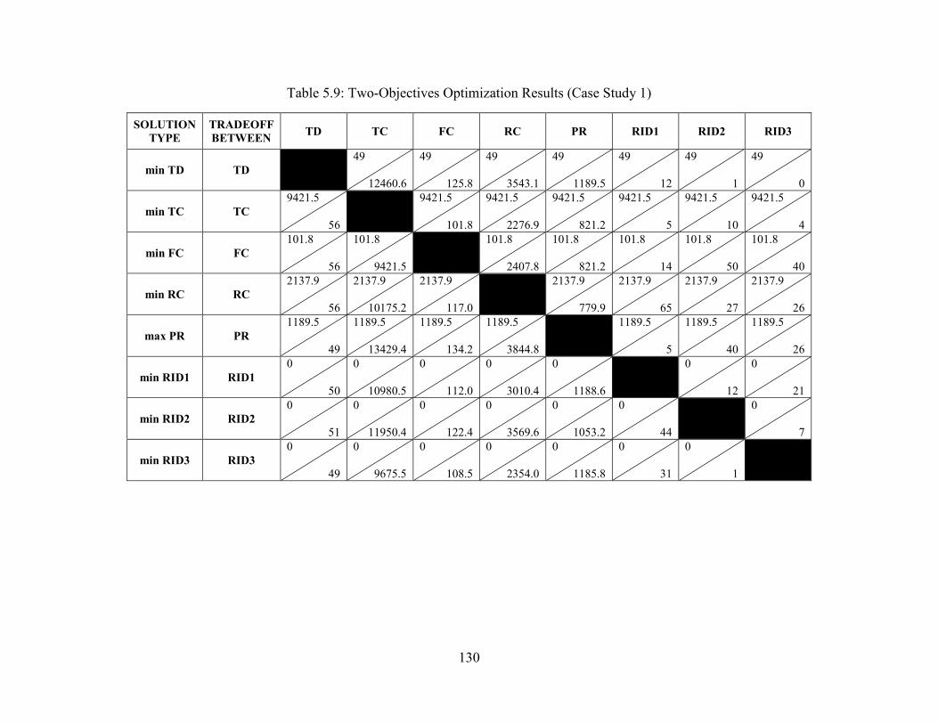
130
Table 5.9: Two-Objectives Optimization Results (Case Study 1)
SOLUTION
TYPE
TRADEOFF
BETWEEN TD TC FC RC PR RID1 RID2 RID3
min TD TD -
49
12460.6
49
125.8
49
3543.1
49
1189.5
49
12
49
1
49
0
min TC TC
9421.5
56
-
9421.5
101.8
9421.5
2276.9
9421.5
821.2
9421.5
5
9421.5
10
9421.5
4
min FC FC
101.8
56
101.8
9421.5
-
101.8
2407.8
101.8
821.2
101.8
14
101.8
50
101.8
40
min RC RC
2137.9
56
2137.9
10175.2
2137.9
117.0
-
2137.9
779.9
2137.9
65
2137.9
27
2137.9
26
max PR PR
1189.5
49
1189.5
13429.4
1189.5
134.2
1189.5
3844.8
-
1189.5
5
1189.5
40
1189.5
26
min RID1 RID1
0
50
0
10980.5
0
112.0
0
3010.4
0
1188.6
-
0
12
0
21
min RID2 RID2
0
51
0
11950.4
0
122.4
0
3569.6
0
1053.2
0
44
-
0
7
min RID3 RID3
0
49
0
9675.5
0
108.5
0
2354.0
0
1185.8
0
31
0
1
-
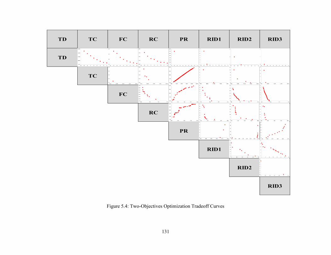
131
TD TC FC RC PR RID1 RID2 RID3
TD
TC
FC
RC
PR
RID1
RID2
RID3
Figure 5.4: Two-Objectives Optimization Tradeoff Curves

132
Using Figure 5.4, the identified set of non-conflicting objectives are as shown in Table
5.10. Those sets help in determining the possible combinations of conflicting objectives
to be optimized together in case more than two objectives are considered for
simultaneous optimization. It should be noted that identified set of non-conflicting
objectives shown in Table 5.10 are specific cases and may vary from project to another as
discussed earlier in Chapter 3. For instance, assume optimizing the following set of
objectives together:
{TD, FC, RC, PR, and RID3}
It will be meaningless to consider the TD with both PR and RID3 under the same set.
Thus, there can be several options to consider. One of those options can be considering
optimizing the TD, FC, and RC together and disregarding both PR and RID3. In other
words, achieving the minimum TD will eventually achieve the minimum RID3 and
maximum PR. Based on that, the main possible tradeoff combinations between all the
objectives together can be summarized as shown in Table 5.11.
Table 5.10: Set of Non-Conflicting Objectives
Set # Non-Conflicting Objectives
1 TD and PR
2 TD and RID3
3 TC and FC

133
Table 5.11: Main-Tradeoff Combination Sets
Main
Tradeoff Set Tradeoff Between Disregarded Objectives
A TD-TC-RC-RID1-RID2 PR, RID3 due to non-confliction with TD
FC due to non-confliction with TC
B TD-FC-RC-RID1-RID2 PR, RID3 due to non-confliction with TD
TC due to non-confliction with FC
C TC-RC-PR-RID1-RID2-RID3 TD due to non-confliction with PR, RID3
FC due to non-confliction with TC
D FC-RC-PR-RID1-RID2-RID3 TD due to non-confliction with PR, RID3
TC due to non-confliction with FC
The tradeoffs shown in Table 5.11 focus on taking the possible maximum number of non-
conflicting objectives to be optimized together. However, more other tradeoffs can be
established by considering only three, four, or five objectives to be simultaneously
optimized depending on the decision maker’s concerns regarding specific objectives. For
example, using the combinations and permutations concept, the main-tradeoff set (A)
(which consists of five objectives) in Table 5.11 can create ten and five sub-tradeoff sets
in which each consists of three and four different objectives, respectively. Thus, a total of
82 unique sub-tradeoff sets varying between three to five objectives are established as
shown in Table 5.12. Having the 82 sub-tradeoff sets as well as the 28-two-objectives
tradeoff sets (Figure 5.4) and the 4 main tradeoff sets (Table 5.11) will result in a total
114 unique tradeoff sets varying from two to six objectives. This gives the contractor a
wide range of tradeoff options to examine based on his/her desired objectives to be
optimized. Generally, the achievement of adequate profit is very essential for
construction business sustainability. Moreover, fluctuations of resources are undesirable
for the contractor as it is expensive to hire and fire labor on a short term basis to satisfy

134
fluctuating resource requirements. Also, controlling the credit limit helps contractors to
avoid progressive cash deficit which can result in difficulties to stick with the planned
schedule. Therefore, balancing these three parameters (i.e. required credit, profit, and
resource fluctuations) is crucial to ensure the achievement of project objectives.
Accordingly, for this case study, the tradeoff set option “C-36” (i.e. RC, PR, RID1, RID2,
and RID3) in Table 5.12 is considered to be optimized using the developed model.
Table 5.12: Main and Sub-Tradeoff Combination Sets
Main
Tradeoff
Set #
No. of
Objectives Tradeoff Between
Sub
Tradeoff
Set #
No. of
Objectives Tradeoff Between
A 5 TD-TC-RC-RID1-RID2
1 3 TD,TC,RC
2 3 TD,TC,RID1
3 3 TD,TC,RID2
4 3 TD,RC,RID1
5 3 TD,RC,RID2
6 3 TD,RID1,RID2
7 3 TC,RC,RID1
8 3 TC,RC,RID2
9 3 TC,RID1,RID2
10 3 RC,RID1,RID2
11 4 TD,TC,RC,RID1
12 4 TD,TC,RC,RID2
13 4 TD,TC,RID1,RID2
14 4 TD,RC,RID1,RID2
15 4 TC,RC,RID1,RID2
B 5 TD-FC-RC-RID1-RID2
1 3 TD,FC,RC
2 3 TD,FC,RID1
3 3 TD,FC,RID2
4 3 FC,RC,RID1
5 3 FC,RC,RID2
6 3 FC,RID1,RID2
7 4 TD,FC,RC,RID1
8 4 TD,FC,RC,RID2
9 4 TD,FC,RID1,RID2
10 4 FC,RC,RID1,RID2
C 6 TC-RC-PR-RID1-RID2-RID3
1 3 TC,RC,PR
2 3 TC,RC,RID3
3 3 TC,PR,RID1
4 3 TC,PR,RID2
5 3 TC,PR,RID3
6 3 TC,RID1,RID3
7 3 TC,RID2,RID3
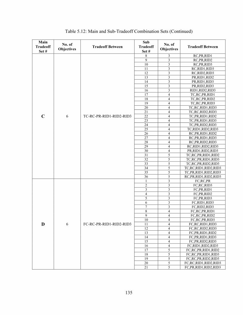
135
Table 5.12: Main and Sub-Tradeoff Combination Sets (Continued)
Main
Tradeoff
Set #
No. of
Objectives Tradeoff Between
Sub
Tradeoff
Set #
No. of
Objectives Tradeoff Between
C 6 TC-RC-PR-RID1-RID2-RID3
8 3 RC,PR,RID1
9 3 RC,PR,RID2
10 3 RC,PR,RID3
11 3 RC,RID1,RID3
12 3 RC,RID2,RID3
13 3 PR,RID1,RID2
14 3 PR,RID1,RID3
15 3 PR,RID2,RID3
16 3 RID1,RID2,RID3
17 4 TC,RC,PR,RID1
18 4 TC,RC,PR,RID2
19 4 TC,RC,PR,RID3
20 4 TC,RC,RID1,RID3
21 4 TC,RC,RID2,RID3
22 4 TC,PR,RID1,RID2
23 4 TC,PR,RID1,RID3
24 4 TC,PR,RID2,RID3
25 4 TC,RID1,RID2,RID3
26 4 RC,PR,RID1,RID2
27 4 RC,PR,RID1,RID3
28 4 RC,PR,RID2,RID3
29 4 RC,RID1,RID2,RID3
30 4 PR,RID1,RID2,RID3
31 5 TC,RC,PR,RID1,RID2
32 5 TC,RC,PR,RID1,RID3
33 5 TC,RC,PR,RID2,RID3
34 5 TC,RC,RID1,RID2,RID3
35 5 TC,PR,RID1,RID2,RID3
36 5 RC,PR,RID1,RID2,RID3
D 6 FC-RC-PR-RID1-RID2-RID3
1 3 FC,RC,PR
2 3 FC,RC,RID3
3 3 FC,PR,RID1
4 3 FC,PR,RID2
5 3 FC,PR,RID3
6 3 FC,RID1,RID3
7 3 FC,RID2,RID3
8 4 FC,RC,PR,RID1
9 4 FC,RC,PR,RID2
10 4 FC,RC,PR,RID3
11 4 FC,RC,RID1,RID3
12 4 FC,RC,RID2,RID3
13 4 FC,PR,RID1,RID2
14 4 FC,PR,RID1,RID3
15 4 FC,PR,RID2,RID3
16 4 FC,RID1,RID2,RID3
17 5 FC,RC,PR,RID1,RID2
18 5 FC,RC,PR,RID1,RID3
19 5 FC,RC,PR,RID2,RID3
20 5 FC,RC,RID1,RID2,RID3
21 5 FC,PR,RID1,RID2,RID3

136
The results of the 9-activity network indicated that the obtained Pareto-optimal front
representing the tradeoff of the five objectives included 125 unique optimal/near optimal
solutions. All of the obtained 125 solutions are non-dominated where no solution is better
than the other with respect to all of the five objectives. In case the contractor do not have
a preference towards a certain objective over the other, then a fuzzy approach can be
utilized to help the decision maker in selecting the best compromise solution/schedule.
Due to the imprecise nature of the decision maker’s judgment, the ith objective function
Oi is represented by a membership function 𝜇𝑖 defined by Dhillon et al. (1993) as shown
in Equations 5.2-5.4.
𝜇𝑖 = 1 𝑂𝑖 ≤ 𝑂𝑖𝑚𝑖𝑛 ………………………………………………………...……...…(5.2)
𝜇𝑖 =𝑂𝑖
𝑚𝑎𝑥−𝑂𝑖
𝑂𝑖𝑚𝑎𝑥−𝑂𝑖
𝑚𝑖𝑛 𝑂𝑖𝑚𝑖𝑛 < 𝑂𝑖 < 𝑂𝑖
𝑚𝑎𝑥........................................................………..…(5.3)
𝜇𝑖 = 0 𝑂𝑖 ≥ 𝑂𝑖𝑚𝑎𝑥 …………………………………………………...…………..…(5.4)
Where 𝑂𝑖𝑚𝑖𝑛 and 𝑂𝑖
𝑚𝑎𝑥= minimum and maximum value of the ith objective function
among all non-dominated solutions, respectively. The membership function value ranges
from 0 to 1. For each non-dominated solution s, the normalized membership function 𝜇𝑠
is calculated as shown in Equation 5.5.
𝜇𝑠 =∑ 𝜇𝑖
𝑠𝑁𝑜𝑏𝑗𝑖=1
∑ ∑ 𝜇𝑖𝑠
𝑁𝑜𝑏𝑗𝑖=1
𝑀𝑠=1
………………………………………...…………………………….(5.5)

137
Where M = number of non-dominated solutions. The best compromise solution is that
having the maximum value of 𝜇𝑠.
Table 5.13 presents six remarkable solutions that exhibit the minimum required credit,
maximum profit, minimum RID1, minimum RID2, minimum RID3, and the best
compromise solution. Such results are obtained by assigning the GAs parameters to 500,
400, 80%, and 10% for the population size, number of generations, crossover probability,
and mutation probability, respectively.
Table 5.13: Five-Objectives Remarkable Solutions (Case Study 1)
Solution Type RC ($) PR ($) RID1 RID2 RID3 TD (days)
Minimum Required Credit (RC) 2,157.3 780.4 66 25 25 56
Maximum Profit (PR) 3,844.8 1,189.5 5 40 26 49
Minimum Resource Idle Days 1 (RID1) 2,564.2 934.4 0 17 31 54
Minimum Resource Idle Days 2 (RID2) 3,571.5 1,048.9 38 0 1 52
Minimum Resource Idle Days 3 (RID3) 2,689.9 1,011.9 62 15 0 55
Best Compromise 3,188.1 1,116.2 44 7 5 52
If the decision maker’s absolute priority is to maximize profit, the solution of the
maximum profit shown in Table 5.13 should be selected wherein the optimization
algorithm selects activities’ start times and execution modes to achieve the global
maximum profit value of $1,189.5, and minimizes, but not globally minimizes, the
required credit and resource fluctuation of the three resources. The minimized required
credit of $3,844.8 in the solution of maximum profit is definitely higher than its global
minimum value of $2,157.3 associated with the solution of minimum required credit

138
shown in Table 5.13. Similarly, the minimized RID1, RID2, and RID3 values of 5, 40,
and 26, respectively in the solution of maximum profit are definitely higher than their
global minimum values of 0, 0, and 0 associated with the solution of minimum RID1,
minimum RID2, and minimum RID3, respectively shown in Table 5.13. In addition to
the solution of maximum profit, the optimization model provides 124 additional
solutions, which represent the complete tradeoff between the required credit, profit, and
resource fluctuation of the three resources. In each one of these solutions, the profit value
is maximized but not globally maximized, the required credit is minimized but not
globally minimized (except for the solution of minimum required credit), and the RID1,
RID2, and RID3 are minimized but not globally minimized (except for the solution of
minimum RID1, minimum RID2, and minimum RID3). As mentioned before, when there
is no reason to favor a particular objective over the other, the best compromise solution
can be selected to achieve a balance between the five objectives.
Figure 5.5 shows the normalized values of the resulted RC, PR, RID1, RID2, and RID3
objectives on five separate vertical axes. The straight lines connecting the normalized
values of the objectives represent the 125 solutions comprising the tradeoff. The non-
dominance condition is fulfilled by violating Equation 3.26, which is graphically
evidenced in Figure 5.5 by the fact that each solution, represented by a broken line
composed of segments, crosses at least one segment of another solution. In addition,
Figure 5.5 shows that the values of the five objectives are well-distributed along the
vertical axis indicating good diversifications of the solutions.
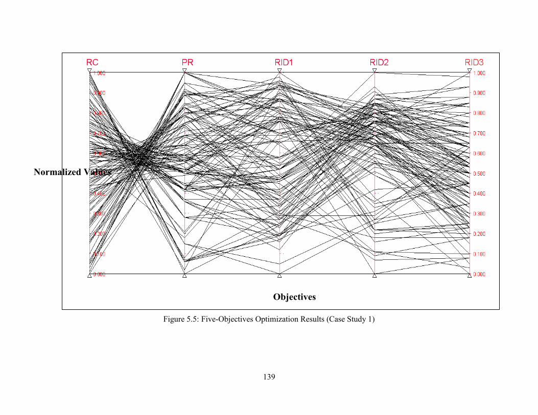
139
Figure 5.5: Five-Objectives Optimization Results (Case Study 1)
Objectives
Normalized Values
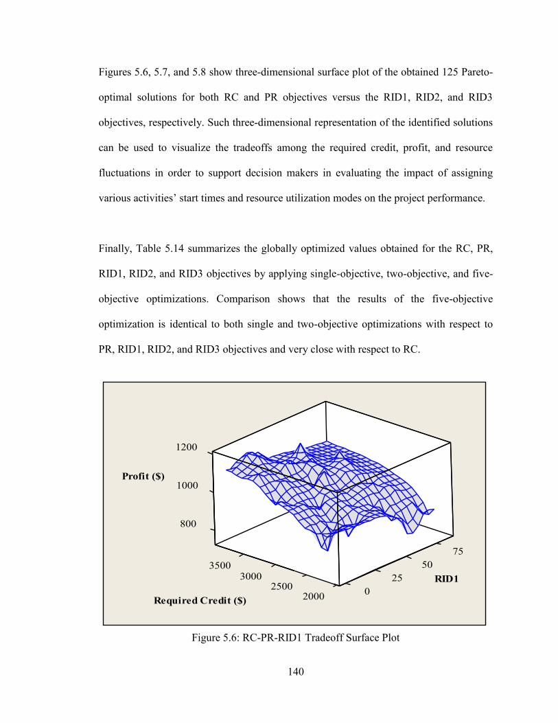
140
800
1000
1200
75
3500 50
3000 252500
02000
Profit ($)
RID1
Required Credit ($)
Figures 5.6, 5.7, and 5.8 show three-dimensional surface plot of the obtained 125 Pareto-
optimal solutions for both RC and PR objectives versus the RID1, RID2, and RID3
objectives, respectively. Such three-dimensional representation of the identified solutions
can be used to visualize the tradeoffs among the required credit, profit, and resource
fluctuations in order to support decision makers in evaluating the impact of assigning
various activities’ start times and resource utilization modes on the project performance.
Finally, Table 5.14 summarizes the globally optimized values obtained for the RC, PR,
RID1, RID2, and RID3 objectives by applying single-objective, two-objective, and five-
objective optimizations. Comparison shows that the results of the five-objective
optimization is identical to both single and two-objective optimizations with respect to
PR, RID1, RID2, and RID3 objectives and very close with respect to RC.
Figure 5.6: RC-PR-RID1 Tradeoff Surface Plot

141
800
1000
60
1200
403500
3000 202500
02000
Profit ($)
RID2
Required Credit ($)
800
1000
45
1200
303500
3000 152500
02000
Profit ($)
RID3
Required Credit ($)
Figure 5.7: RC-PR-RID2 Tradeoff Surface Plot
Figure 5.8: RC-PR-RID3 Tradeoff Surface Plot

142
Table 5.14: Summary of Optimization Results (Case Study 1)
Objectives
SINGLE
Objective
Optimization
TWO
Objective
Optimization
FIVE
Objective
Optimization
RC ($) 2,137.9 2,137.9 2,157.3
PR ($) 1,189.5 1,189.5 1,189.5
RID1 0 0 0
RID2 0 0 0
RID3 0 0 0
5.2.2 Case Study (2): 25 and 30-Activity Multiple Projects
The second case study uses an example of two concurrent projects of 25 and 30 activities
adopted from Abido and Elazouni (2011). The problem was originally solved to optimize
the tradeoff between the objectives of total duration, financing cost, and required credit
under single resource utilization mode considering no resource levelling and allocation.
The CPM networks of the 25 and 30 activity project are shown in Figures 5.9 and 5.10,
respectively. Similar to the first case study, the problem is to be solved considering both
financial and resource aspects. Thus, the objectives selected to be optimized
simultaneously will consider maximizing the profit (PR) while minimizing the required
credit (RC) and resource fluctuation and peak demand (RFPD). However, this time the
RFPD objective will consider both resource allocation and levelling using the RRH
metric under constrained resource limit. Hence, Equation 3.18a is used to determine the
RFPD by assigning the RRH weight factor (W1) and MRD weight factor (W2) a value of
0.5 each. Moreover, two execution modes are assumed for most of the activities in both
projects. The time period used for both projects is in weeks where each week is assumed
to have five working days. The two projects were set up such that the start of the 30-
activity project is shifted three weeks behind the start of the 25-activity project (i.e. day

143
START FINISH
A
B
C
D
E
F
G
H
I
J
K
L
M
N
O
P
Q
R
S
T
U
V
W
X
Y
Aa Ab Ac Ad Ae
Ba Bb Bc Bd Be
Ca Cb Cc Cd Ce
Da Db Dc Dd De
Fa Fb Fc Fd Fe
Ea Eb Ec Ed Ee
15). The time, financial, and contractual terms data of the two projects are as shown in
Table 5.15.
Figure 5.9: 25-Activity Project CPM Network
Figure 5.10: 30-Activity Project CPM Network
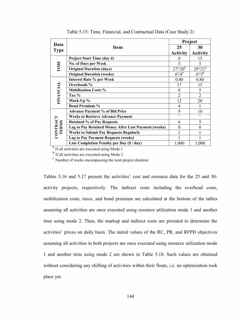
144
Table 5.15: Time, Financial, and Contractual Data (Case Study 2)
Data
Type Item
Project
25
Activity
30
Activity
TIM
E Project Start Time (day #) 0 15
No. of Days per Week 5 5 Original Duration (days) 27
a/20
b 29
a/21
b
Original Duration (weeks) 6a/4
b 6
a/5
b
FIN
AN
CIA
L Interest Rate % per Week 0.80 0.80
Overheads % 17 15 Mobilization Costs % 8 5 Tax % 2 2 Mark-Up % 12 20 Bond Premium % 4 1
CO
NT
RA
CT
TE
RM
S
Advance Payment % of Bid Price 9 10 Weeks to Retrieve Advance Payment c c
Retained % of Pay Requests 6 5 Lag to Pay Retained Money After Last Payment (weeks) 0 0 Weeks to Submit Pay Requests Regularly 1 1 Lag to Pay Payment Requests (weeks) 1 1 Late Completion Penalty per Day ($ / day) 1,000 1,000
a If all activities are executed using Mode 1
b If all activities are executed using Mode 2
c Number of weeks encompassing the total project duration
Tables 5.16 and 5.17 present the activities’ cost and resource data for the 25 and 30-
activity projects, respectively. The indirect costs including the overhead costs,
mobilization costs, taxes, and bond premium are calculated at the bottom of the tables
assuming all activities are once executed using resource utilization mode 1 and another
time using mode 2. Then, the markup and indirect costs are prorated to determine the
activities’ prices on daily basis. The initial values of the RC, PR, and RFPD objectives
assuming all activities in both projects are once executed using resource utilization mode
1 and another time using mode 2 are shown in Table 5.18. Such values are obtained
without considering any shifting of activities within their floats, i.e. no optimization took
place yet.

145
Table 5.16: Cost and Resource Data (25-Activity Project)
Activity
MODE 1 MODE 2
Duration
(days)
Daily
Direct
Cost
($/day)
Daily
Price
($/day)
Daily
Resources
Duration
(days)
Daily
Direct
Cost
($/day)
Daily
Price
($/day)
Daily
Resources
A 2 1000 1501.28 3 1 1600 2402.04 4
B 3 1200 1801.53 2 2 1800 2702.30 3
C 2 1100 1651.41 1 1 2200 3302.81 2
D 3 900 1351.15 4 2 1300 1951.66 5
E 3 1250 1876.60 2 2 1950 2927.49 3
F 3 1150 1726.47 2 2 1850 2777.36 3
G 2 1050 1576.34 5 1 1350 2026.73 6
H 3 950 1426.21 2 1 2000 3002.56 4
I 2 650 975.83 5 1 950 1426.21 6
J 5 450 675.58 1 3 1250 1876.60 3
K 5 350 525.45 1 4 700 1050.89 2
L 5 500 750.64 2 4 850 1276.09 3
M 1 1450 2176.85 5 - - - -
N 5 400 600.51 5 3 700 1050.89 7
O 5 550 825.70 5 4 850 1276.09 6
P 4 500 750.64 4 3 750 1125.96 5
Q 3 1350 2026.73 2 2 1900 2852.43 3
R 5 600 900.77 5 4 800 1201.02 6
S 5 850 1276.09 4 4 1200 1801.53 5
T 6 700 1050.89 3 4 1500 2251.92 5
U 4 1200 1801.53 2 3 1800 2702.30 3
V 3 1850 2777.36 1 2 3400 5104.35 2
W 5 650 975.83 4 4 900 1351.15 5
X 5 600 900.77 2 4 1050 1576.34 3
Y 2 1000 1501.28 1 1 1800 2702.30 2
Mode 1:
Total Cash Outflow = 72,750; Overheads = 12,367.5; Mobilization = 6,809.4; Cash Outflow + Overheads +
Mobilization = 91,926.9; Taxes = 1,838.5; Taxes + Cash Outflow + Overheads + Mobilization = 93,765.4;
Markup = 11,251.9; Markup + Taxes + Cash Outflow + Overheads + Mobilization = 105,017.3; Bond
Premium = 4,200.7; Total Bid Price = 109,218; and Bid Price Factor (109,218 / 72,750) = 1.50128.
Mode 2:
Total Cash Outflow = 80,650; Overheads = 13,710.5; Mobilization = 7,548.8; Cash Outflow + Overheads +
Mobilization = 101,909.3; Taxes = 2,038.2; Taxes + Cash Outflow + Overheads + Mobilization =
103,947.5; Markup = 12,473.7; Markup + Taxes + Cash Outflow + Overheads + Mobilization = 116,421.2;
Bond Premium = 4,656.9; Total Bid Price = 1021,078; and Bid Price Factor (121,078 / 80,650) = 1.50128.
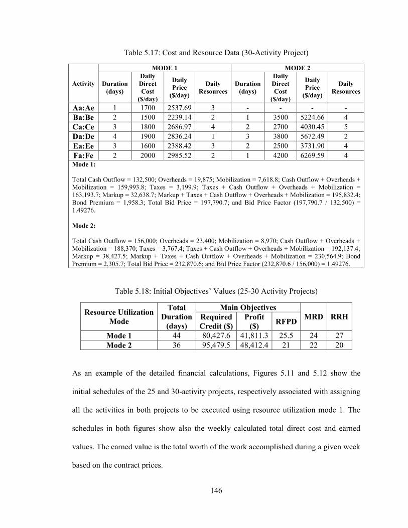
146
Table 5.17: Cost and Resource Data (30-Activity Project)
Activity
MODE 1 MODE 2
Duration
(days)
Daily
Direct
Cost
($/day)
Daily
Price
($/day)
Daily
Resources
Duration
(days)
Daily
Direct
Cost
($/day)
Daily
Price
($/day)
Daily
Resources
Aa:Ae 1 1700 2537.69 3 - - - -
Ba:Be 2 1500 2239.14 2 1 3500 5224.66 4
Ca:Ce 3 1800 2686.97 4 2 2700 4030.45 5
Da:De 4 1900 2836.24 1 3 3800 5672.49 2
Ea:Ee 3 1600 2388.42 3 2 2500 3731.90 4
Fa:Fe 2 2000 2985.52 2 1 4200 6269.59 4
Mode 1:
Total Cash Outflow = 132,500; Overheads = 19,875; Mobilization = 7,618.8; Cash Outflow + Overheads +
Mobilization = 159,993.8; Taxes = 3,199.9; Taxes + Cash Outflow + Overheads + Mobilization =
163,193.7; Markup = 32,638.7; Markup + Taxes + Cash Outflow + Overheads + Mobilization = 195,832.4;
Bond Premium = 1,958.3; Total Bid Price = 197,790.7; and Bid Price Factor (197,790.7 / 132,500) =
1.49276.
Mode 2:
Total Cash Outflow = 156,000; Overheads = 23,400; Mobilization = 8,970; Cash Outflow + Overheads +
Mobilization = 188,370; Taxes = 3,767.4; Taxes + Cash Outflow + Overheads + Mobilization = 192,137.4;
Markup = 38,427.5; Markup + Taxes + Cash Outflow + Overheads + Mobilization = 230,564.9; Bond
Premium = 2,305.7; Total Bid Price = 232,870.6; and Bid Price Factor (232,870.6 / 156,000) = 1.49276.
Table 5.18: Initial Objectives’ Values (25-30 Activity Projects)
Resource Utilization
Mode
Total
Duration
(days)
Main Objectives
MRD RRH Required
Credit ($)
Profit
($) RFPD
Mode 1 44 80,427.6 41,811.3 25.5 24 27
Mode 2 36 95,479.5 48,412.4 21 22 20
As an example of the detailed financial calculations, Figures 5.11 and 5.12 show the
initial schedules of the 25 and 30-activity projects, respectively associated with assigning
all the activities in both projects to be executed using resource utilization mode 1. The
schedules in both figures show also the weekly calculated total direct cost and earned
values. The earned value is the total worth of the work accomplished during a given week
based on the contract prices.
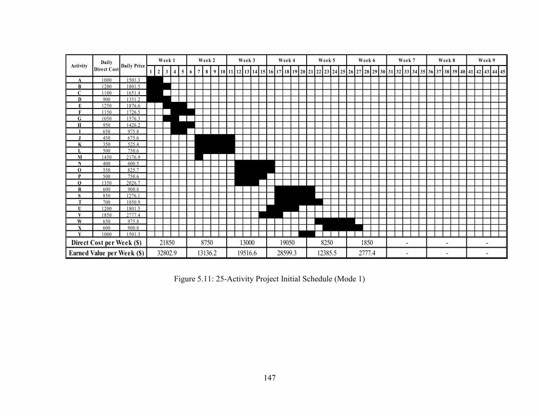
147
1 2 3 4 5 6 7 8 9 10 11 12 13 14 15 16 17 18 19 20 21 22 23 24 25 26 27 28 29 30 31 32 33 34 35 36 37 38 39 40 41 42 43 44 45
A 1000 1501.3
B 1200 1801.5
C 1100 1651.4
D 900 1351.2
E 1250 1876.6
F 1150 1726.5
G 1050 1576.3
H 950 1426.2
I 650 975.8
J 450 675.6
K 350 525.4
L 500 750.6
M 1450 2176.9
N 400 600.5
O 550 825.7
P 500 750.6
Q 1350 2026.7
R 600 900.8
S 850 1276.1
T 700 1050.9
U 1200 1801.5
V 1850 2777.4
W 650 975.8
X 600 900.8
Y 1000 1501.3
Daily
Direct CostDaily Price
Week 8 Week 9Activity
Week 1 Week 2 Week 3 Week 4 Week 5 Week 6 Week 7
Direct Cost per Week ($)
Earned Value per Week ($)
21850 8750 13000 -
32802.9 13136.2 19516.6 28599.3 12385.5 2777.4 - - -
19050 8250 1850 - -
Figure 5.11: 25-Activity Project Initial Schedule (Mode 1)

148
1 2 3 4 5 6 7 8 9 10 11 12 13 14 15 16 17 18 19 20 21 22 23 24 25 26 27 28 29 30 31 32 33 34 35 36 37 38 39 40 41 42 43 44 45
Aa 1700 2537.7
Ab 1700 2537.7
Ac 1700 2537.7
Ad 1700 2537.7
Ae 1700 2537.7
Ba 1500 2239.1
Bb 1500 2239.1
Bc 1500 2239.1
Bd 1500 2239.1
Be 1500 2239.1
Ca 1800 2687.0
Cb 1800 2687.0
Cc 1800 2687.0
Cd 1800 2687.0
Ce 1800 2687.0
Da 1900 2836.2
Db 1900 2836.2
Dc 1900 2836.2
Dd 1900 2836.2
De 1900 2836.2
Ea 1600 2388.4
Eb 1600 2388.4
Ec 1600 2388.4
Ed 1600 2388.4
Ee 1600 2388.4
Fa 2000 2985.5
Fb 2000 2985.5
Fc 2000 2985.5
Fd 2000 2985.5
Fe 2000 2985.5
Week 5 Week 6 Week 7 Week 8 Week 9
Direct Cost per Week ($) - - -
Week 4Activity
Daily
Direct CostDaily Price
Week 1 Week 2 Week 3
Earned Value per Week ($) - - - 35229.1
23600 30400 22100 20000 7200
45379.9 32990.0 29855.2 10747.9
29200
43588.6
Figure 5.12: 30-Activity Project Initial Schedule (Mode 1)
149
Table 5.19 presents the weekly cash outflow Et and inflow Pt calculations of the
individual projects and the two projects together. The calculations of Et incorporates the
mobilization and bond which occur at the beginning of the projects whereas the
calculations of Pt incorporates the advance payment at the beginning of the projects, and
the retained percentage applied to the payments. For clarification purposes, assume the
25-activity project schedule shown in Figure 5.11 is delayed 2 days. Accordingly, a late
completion penalty is to be applied by assigning an extra amount of $ 2,000 (i.e. 2 x
1,000) in the “deductions” cell at the end of week 7 in Table 5.19. Consequently, the Et
and Pt values of the two projects together are used to determine the other financial
parameters as shown in Table 5.20. Moreover, Figure 5.13 shows the net cash flow
diagram associated with the financial parameters obtained in Table 5.20.
Three runs of single-objective optimization are done to optimize the RC, PR, and RFPD
objectives individually considering no resource limit constraint. The achieved optimized
objectives’ value from the single-objective optimization runs is shown in Table 5.21.
Each of those individually optimized objectives’ value represents a unique start times of
the activities having a unique selected execution mode. The initial three objectives values
ranged from $80,427.6 to $95,479.5, $41,811.3 to $48,412.4, and 21 to 25.5, for the RC,
PR, and RFPD, respectively as shown in Table 5.18. The results in Table 5.21 show a
significant improvement in both the RC and RFPD objectives being minimized to
$49,026.9 and 12.5, respectively. Such improvement is achieved by improving the initial
population through several successive generations in which both the activities’ start times
and execution modes are optimally assigned using the NSGA-II technique in the

150
developed model. However, the PR improvement is insignificant due to the fact of all
activities being assigned to mode 2 (having higher costs thus higher mark-up) was
already done in Table 5.18.
Consequently, another run is done to optimize the three objectives simultaneously
assuming a daily maximum resource demand of 18. The results indicated that the
obtained Pareto-optimal front representing the tradeoff of the three objectives included 67
unique optimal/near optimal non-dominated solutions. Table 5.22 presents four
remarkable solutions that exhibit the minimum RC, maximum PR, minimum RFPD, and
the best compromise solution. Such results are obtained by assigning the GAs parameters
to 800, 600, 90%, and 15% for the population size, number of generations, crossover
probability, and mutation probability, respectively. The average processing time to solve
the problem was around 3 hours using a desktop of 3.2 GHz processor speed and 8 GB
RAM. As seen in Table 5.22, the maximum resource demand in all types of solution did
not exceed the set resource limit, i.e. 18.

151
Table 5.19: Initial Weekly Cash Outflow and Inflow Calculations (Mode 1)
End
of
Week
Cash Outflow (Et) Cash Inflow (Pt)
Item 25-Act.
Project
30-Act.
Project
Sum
of Two
Projects
Item 25-Act.
Project
30-Act.
Project
Sum
of Two
Projects
0 Mobilization & Bond 11230.3e
- 11230.3 Advance Payment 9829.6f
- 9829.6
1
Direct Cost 21850 - - Earned Value - - -
Overhead 2061.25a - - Deductions - - -
Tax 478.23b
- - Additions - - -
Total 24389.5 - 24389.5 Net - - -
2
Direct Cost 8750 - - Earned Value 32802.9 - -
Overhead 2061.25a - - Deductions 4920.4
c - -
Tax 216.23b
- - Additions - - -
Total 11027.5 - 11027.5 Net 27882.5 - 27882.5
3
Direct Cost 13000 - - Earned Value 13136.2 - -
Overhead 2061.25a - - Deductions 1970.4
c - -
Tax 301.23b
- - Additions - - -
Total 15362.5 9768.6e
25131.1 Net 11165.8 19779f
30944.8
4
Direct Cost 19050 23600 - Earned Value 19516.6 - -
Overhead 2061.25a 3312.5
a - Deductions 2927.5
c - -
Tax 422.23b
538.25b
- Additions - - -
Total 21533.5 27450.8 48984.2 Net 16589.1 - 16589.1
5
Direct Cost 8250 29200 - Earned Value 28599.3 35229.1 -
Overhead 2061.25a 3312.5
a - Deductions 4289.9
c 5284.4
c -
Tax 206.23b
650.25b
- Additions - - -
Total 10517.5 33162.8 43680.2 Net 24309.4 29944.7 54254.1
6
Direct Cost 1850 30400 - Earned Value 12385.5 43588.6 -
Overhead 2061.25a 3312.5
a - Deductions 1857.8
c 6538.3
c -
Tax 78.23b
674.25b
- Additions - - -
Total 3989.5 34386.8 38376.2 Net 10527.7 37050.3 47578
7
Direct Cost - 22100 - Earned Value 2777.4 45379.9 -
Overhead -
3312.5a
- Deductions 416.6c
6807c
-
Tax -
508.25b
- Additions 6553.1d
- -
Total - 34284.8 25920.8 Net 8913.9 38572.9 47486.8
8
Direct Cost - 20000 - Earned Value - 32990.0 -
Overhead - 3312.5a
- Deductions -
4948.5c
-
Tax - 466.25b
- Additions -
- -
Total - 23778.8 23778.8 Net - 28041.5 28041.5
9
Direct Cost - 7200 - Earned Value - 29855.2 -
Overhead - 3312.5a
- Deductions - 4478.3c
-
Tax - 210.25b
- Additions - - -
Total - 10722.8 10722.8 Net - 25376.9 25376.9
10
Direct Cost - - - Earned Value - 10747.9 -
Overhead - - - Deductions - 1612.2c
-
Tax - - - Additions - 9889.5d
-
Total - - - Net - 19025.2 19025.2 a Overhead per week = Total Overheads / Original duration in weeks
b Tax = (Tax %) x (Direct Cost + Overhead)
c Deductions = (Retained % + Advance Payment %) x Earned Value
d Additions = Total Retained Money
e (Mobilization + Bond) x (1 + Tax %)
f (Advance Payment %) x Total Bid Price

152
Table 5.20: Initial Financial Parameters Calculations (Mode 1)
Week # 0 1 2 3 4 5 6 7 8 9 10
Final E values (E) -11230.3 -24389.5 -11027.5 -25131.1 -48984.2 -43680.2 -38376.2 -25920.8 -23778.8 -10722.8 0.0
Final P values (P) 9829.6 0.0 27882.5 30944.8 16589.1 54254.2 47578.0 47486.8 28041.5 25376.9 19025.2
Cumulative Balance (F) -11230.3 -25790.1 -36817.6 -34066.2 -52105.6 -79196.7 -63318.8 -41661.5 -17953.5 -634.8 24742.2
Cumulative Net Balance (N) -1400.7 -25790.1 -8935.1 -3121.4 -35516.5 -24942.5 -15740.8 5825.3 10088.0 24742.2 43767.4
Financing Cost (I) -5.6 -108.8 -250.4 -172.0 -220.9 -458.9 -353.0 -229.6 -71.8 -2.5 0.0
Compounded Financing Cost (I’) -5.6 -114.4 -365.8 -540.7 -765.9 -1230.9 -1593.8 -1836.2 -1922.7 -1940.6 -1956.1
Cumulative Balance Including Financing Cost (F’) -11235.9 -25904.6 -37183.4 -34606.9 -52871.6 -80427.6 -64912.6 -43497.7 -19876.2 -2575.3 22786.1
Cumulative Net Balance Including Financing Cost (N’) -1406.3 -25904.6 -9300.9 -3662.1 -36282.4 -26173.4 -17334.5 3989.1 8165.3 22801.6 41811.3

153
Figure 5.13: Initial Net Cash Flow (Mode 1)
-11235.9
-1406.3
-25904.6
-37183.4
-9300.9
-34606.9
-3662.1
-52871.6
-36282.4
-80427.6
-26173.4
-64912.6
-17334.5
-43497.7
3989.1
-19876.2
8165.3
-2575.3
22801.6
22786.1
41811.3
-90,000
-70,000
-50,000
-30,000
-10,000
10,000
30,000
50,000
0 1 2 3 4 5 6 7 8 9 10
CA
SH
FL
OW
($)
WEEK #

154
Table 5.21: Single-Objective Optimization Results (Case Study 2)
Objective Optimized
Value MRD RRH
RC ($) 49,026.9 18 23
PR ($) 48,431.1 22 35
RFPD 12.5 18 7
Table 5.22: Three-Objectives Remarkable Solutions (Case Study 2)
Solution Type Main Objectives
MRD RRH TD
(days) RC ($) PR ($) RFPD
Minimum Required Credit (RC) 50,281.2 46,354.4 24 18 30 44
Maximum Profit (PR) 68,706 47,313.8 29 18 40 40
Minimum RFPD 60,765.4 43,144.4 13 18 8 44
Best Compromise 52,452.4 46,549.1 15.5 17 14 42
As discussed in the first case study, if the decision maker’s absolute priority is to
maximize profit, the solution of the maximum profit shown in Table 5.22 should be
selected wherein the optimization algorithm selects activities’ start times and execution
modes to achieve the global maximum profit value of $47,313.8, and minimizes, but not
globally minimizes, the required credit and resource fluctuation and peak demand. The
minimized required credit of $68,706 in the solution of maximum profit is definitely
higher than its global minimum value of $50,281.2 associated with the solution of
minimum required credit shown in Table 5.22. Similarly, the minimized RFPD value of
29 in the solution of maximum profit is definitely higher than its global minimum value
of 13 associated with the solution of minimum RFPD shown in Table 5.22. In addition to
the solution of maximum profit, the optimization model provides 66 additional solutions,
which represent the complete tradeoff between the required credit, profit, and resource
fluctuation and peak demand. In each one of these solutions, the profit value is
maximized but not globally maximized, the required credit is minimized but not globally
minimized (except for the solution of minimum required credit), and the RFPD is

155
minimized but not globally minimized (except for the solution of minimum RFPD).
Figure 5.14 shows the comparison of the net cash flow obtained from the “minimum RC”
solution (see Table 5.22) to that obtained for the two cases presented in Table 5.18. The
figure shows the significant improvement in minimizing the required credit when
compared with the initial schedules’ results. Similarly, Figure 5.15 shows the comparison
of the resource demand profile obtained from the “minimum RFPD” solution (see Table
5.22) to that obtained for the two cases presented in Table 5.18. Again, the figure shows
the significant improvement in minimizing the resource fluctuations as well as
minimizing the maximum daily resource demand by not exceeding the resource limit of
18 when compared with the initial schedules’ results. Figure 5.16 shows the three-
dimensional surface plot of the obtained 67 Pareto-optimal solutions.

156
Figure 5.14: Net Cash Flows Comparison
-80,428
-95,479
-50,281
-100,000
-80,000
-60,000
-40,000
-20,000
0
20,000
40,000
60,000
0 1 2 3 4 5 6 7 8 9 10
CA
SH
FL
OW
($)
WEEK #
Initial Net Cash Flow (Mode 1) Initial Net Cash Flow (Mode 2) Optimized Net Cash Flow
Maximum
Required
Credit

157
0
5
10
15
20
25
1 2 3 4 5 6 7 8 9 10 11 12 13 14 15 16 17 18 19 20 21 22 23 24 25 26 27 28 29 30 31 32 33 34 35 36 37 38 39 40 41 42 43 44
To
tal
Da
ily
Res
ou
rce D
ema
nd
Day #
Initial Resource Demand Profile (Mode 1)
Resource Limit = 18
0
5
10
15
20
25
1 2 3 4 5 6 7 8 9 10 11 12 13 14 15 16 17 18 19 20 21 22 23 24 25 26 27 28 29 30 31 32 33 34 35 36 37 38 39 40 41 42 43 44
To
tal
Da
ily
Res
ou
rce D
ema
nd
Day #
Initial Resource Demand Profile (Mode 2)
Resource Limit = 18
0
5
10
15
20
25
1 2 3 4 5 6 7 8 9 10 11 12 13 14 15 16 17 18 19 20 21 22 23 24 25 26 27 28 29 30 31 32 33 34 35 36 37 38 39 40 41 42 43 44
To
tal
Da
ily
Res
ou
rce D
ema
nd
Day #
Optimized Resource Demand Profile
Resource Limit = 18
Figure 5.15: Resource Demand Profiles Comparison

158
80000
42000
44000
46000
70000
48000
15
2060000
2550000 30
Profit ($)
Required Credit ($)RFPD
A final run is done again to optimize the three objectives simultaneously assuming a daily
maximum resource demand of 18. However, in this run, an extension increment of 15
days is assumed for both the 25 and 30 activity projects. Such extension intends to further
minimize the required credit. The final results included 139 unique optimal/near optimal
non-dominated solutions Table 5.23 presents the four remarkable solutions that exhibit
the minimum RC, maximum PR, minimum RFPD, and the best compromise solution
after applying the projects’ extension scheme. Figure 5.17 shows the three-dimensional
surface plot of the obtained 139 Pareto-optimal solutions after applying the projects’
extension scheme.
Figure 5.16: RC-PR-RFPD Tradeoff Surface Plot (Case Study 2)
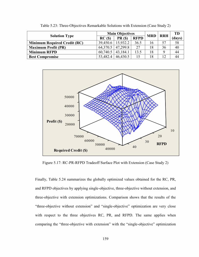
159
10
20000
30000
70000 20
40000
50000
60000 3050000
4040000
Profit ($)
RFPD
Required Credit ($)
Table 5.23: Three-Objectives Remarkable Solutions with Extension (Case Study 2)
Solution Type Main Objectives
MRD RRH TD
(days) RC ($) PR ($) RFPD
Minimum Required Credit (RC) 39,450.6 15,932.2 36.5 16 57 58
Maximum Profit (PR) 64,370.5 47,299.8 27 18 36 40
Minimum RFPD 60,740.5 43,184.1 13.5 18 9 44
Best Compromise 53,482.4 46,430.5 15 18 12 44
Figure 5.17: RC-PR-RFPD Tradeoff Surface Plot with Extension (Case Study 2)
Finally, Table 5.24 summarizes the globally optimized values obtained for the RC, PR,
and RFPD objectives by applying single-objective, three-objective without extension, and
three-objective with extension optimizations. Comparison shows that the results of the
“three-objective without extension” and “single-objective” optimization are very close
with respect to the three objectives RC, PR, and RFPD. The same applies when
comparing the “three-objective with extension” with the “single-objective” optimization

160
except for the RC. As shown in Table 5.24, the required credit is significantly improved
being minimized to $39,450.6 after applying the extension scheme for the 25 and 30-
activity projects. However, such improvement imposed a major reduction in the profit
with a value of $15,932.2 as shown in Table 5.23. This reduction usually happens when
projects are extended beyond their original duration due to the additional overheads and
liquidated damages. Figure 5.18 illustrates the improvement achieved in minimizing the
required credit before and after applying the extension increment and its effect on the
total profit.
Table 5.24: Summary of Optimization Results (Case Study 2)
Optimization
Type Objective
Optimized
Value MRD RRH
Single-Objective
RC ($) 49,026.9 18 23
PR ($) 48,431.1 22 35
RFPD 12.5 18 7
Three-Objective
(Without
Extension)
RC ($) 50,281.2 18 30
PR ($) 47,313.8 18 40
RFPD 13 18 8
Three-Objective
(With Extension)
RC ($) 39,450.6 16 57
PR ($) 47,299.8 18 36
RFPD 13.5 18 9
5.2.3 Case Study (3): 100 and 120-Activity Multiple Projects
The final case study uses the same example of the two concurrent projects of 25 and 30
activities that were presented in the second case study. However, to investigate the
scalability of the developed model, these two projects are enlarged to two bigger projects
of 100 and 120 activities. The 25-activity project was copied into a 100-activity project
by repeating the network in Figure 5.9 four times such that activities A, B, C, and D of
any network depend on activities W, X, Y, and V of the previous network, respectively.
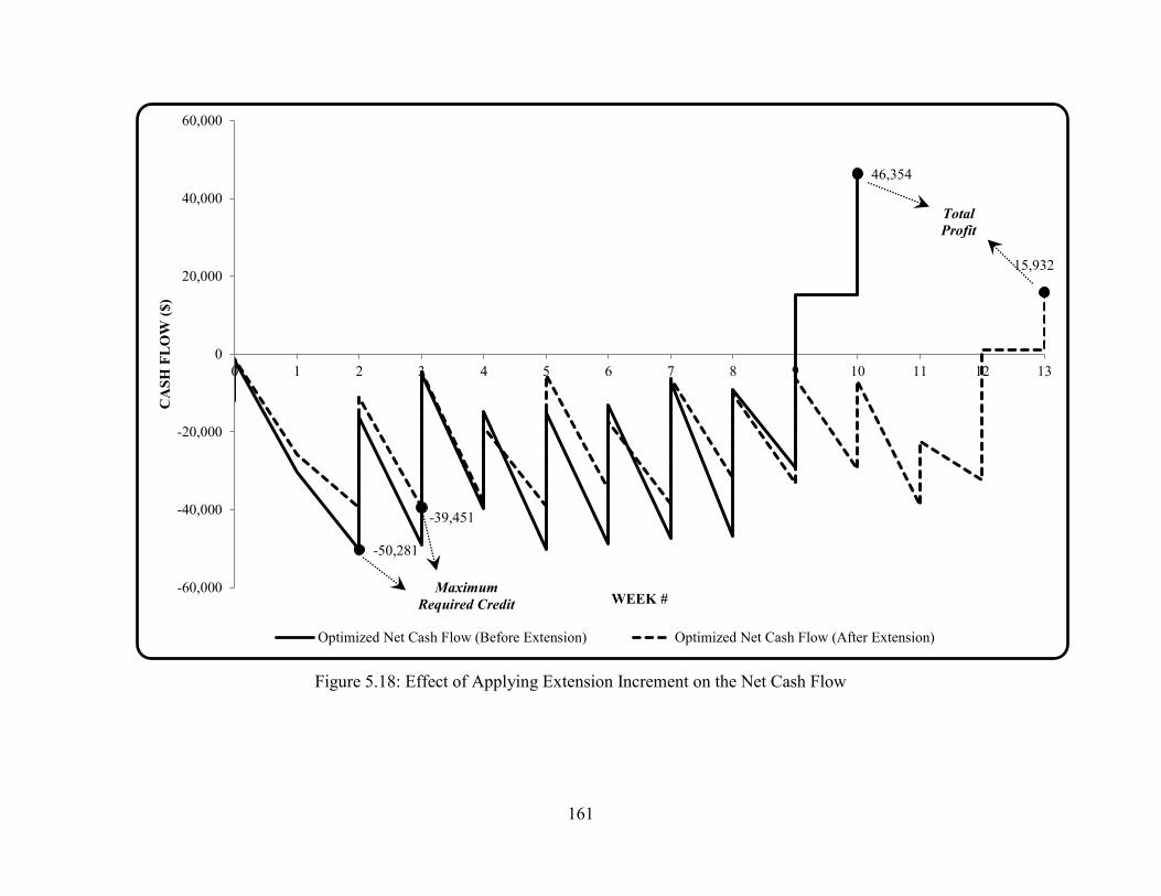
161
Figure 5.18: Effect of Applying Extension Increment on the Net Cash Flow
-50,281
46,354
-39,451
15,932
-60,000
-40,000
-20,000
0
20,000
40,000
60,000
0 1 2 3 4 5 6 7 8 9 10 11 12 13
CA
SH
FL
OW
($
)
WEEK #
Optimized Net Cash Flow (Before Extension) Optimized Net Cash Flow (After Extension)
Maximum
Required Credit
Total
Profit

162
The 30-activity project was expanded into a 120-activity project by repeating the basic
six activities A, B, C, D, E, and F (Figure 5.10) over 15 more sections. The two projects
were set up such that the start of the 120-activity project is shifted eight weeks behind the
start of the 100-activity project (i.e. day 40). The time, financial, and contractual terms
data of the two projects are as shown in Table 5.25.
Table 5.25: Time, Financial, and Contractual Data (Case Study 3)
Data
Type Item
Project
25
Activity
30
Activity
TIM
E Project Start Time (day #) 0 40
No. of Days per Week 5 5 Original Duration (days) 108
a/80
b 89
a/66
b
Original Duration (weeks) 22a/16
b 18
a/14
b
FIN
AN
CIA
L Interest Rate % per Week 0.80 0.80
Overheads % 15 15 Mobilization Costs % 2 2 Tax % 2 2 Mark-Up % 15 15 Bond Premium % 1 1
CO
NT
RA
CT
TE
RM
S
Advance Payment % of Bid Price 6 8 Weeks to Retrieve Advance Payment c c
Retained % of Pay Requests 5 5 Lag to Pay Retained Money After Last Payment (weeks) 0 0 Weeks to Submit Pay Requests Regularly 1 1 Lag to Pay Payment Requests (weeks) 1 1 Late Completion Penalty per Day ($ / day) 1,000 1,000
a If all activities are executed using Mode 1
b If all activities are executed using Mode 2
c Number of weeks encompassing the total project duration
The initial values of the RC, PR, and RFPD objectives assuming all activities in both
projects are once executed using resource utilization mode 1 and another time using
mode 2 are shown in Table 5.26. Such values are obtained considering the early start
times of the activities.

163
Table 5.26: Initial Objectives’ Values (100-120 Activity Projects)
Resource Utilization
Mode
Total
Duration
(days)
Main Objectives
MRD RRH Required
Credit ($)
Profit
($) RFPD
Mode 1 129 69,848.6 144,666.8 87 33 141
Mode 2 106 141,044.6 165,228.3 79 40 118
Similar to the second case study, three runs of single-objective optimization is done to
optimize the RC, PR, and RFPD objectives individually considering no resource limit
constraint. The achieved optimized objectives’ value from the single-objective
optimization runs is shown in Table 5.27. The initial three objectives values ranged from
$69,848.6 to $141,044.6, $144,666.8 to $165,228.3, and 79 to 87, for the RC, PR, and
RFPD, respectively as shown in Table 5.26. The results in Table 5.27 show a significant
improvement in both the RC and RFPD objectives being minimized to $42,411.8 and
70.5, respectively. However, the PR improvement is insignificant due to the fact of all
activities being assigned to mode 2 (having higher costs thus higher mark-up) was
already done in Table 5.26.
Table 5.27: Single-Objective Optimization Results (Case Study 3)
Objective Optimized
Value MRD RRH
RC ($) 42,411.8 29 204
PR ($) 165,372.7 41 197
RFPD 70.5 29 112
Consequently, another run is done to optimize the three objectives simultaneously
assuming a daily maximum resource demand of 29. The results indicated that the
obtained Pareto-optimal front representing the tradeoff of the three objectives included
151 unique optimal/near optimal non-dominated solutions. Table 5.28 presents four

164
80000
140000
80
150000
70000
160000
60000 100
50000 120
Profit ($)
RFPD
Required Credit ($)
remarkable solutions that exhibit the minimum RC, maximum PR, minimum RFPD, and
the best compromise solution. Such results are obtained by assigning the GAs parameters
to 1200, 1000, 90%, and 20% for the population size, number of generations, crossover
probability, and mutation probability, respectively. The average processing time to solve
the problem was around 33.4 hours using a desktop of 3.2 GHz processor speed and 8 GB
RAM. As seen in Table 5.28, the maximum resource demand in all types of solution did
not exceed the set resource limit, i.e. 29. Figure 5.19 shows the three-dimensional surface
plot of the obtained 151 Pareto-optimal solutions.
Table 5.28: Three-Objectives Remarkable Solutions (Case Study 3)
Solution Type Main Objectives
MRD RRH TD
(days) RC ($) PR ($) RFPD
Minimum Required Credit (RC) 42,430.7 141,487.7 113 29 127 129
Maximum Profit (PR) 76,285.9 158,137.6 104 29 179 120
Minimum RFPD 56,252.7 148,456.3 72 29 115 127
Best Compromise 45,474.5 151,068.0 84.5 29 140 129
Figure 5.19: RC-PR-RFPD Tradeoff Surface Plot (Case Study 3)

165
50000
80000
100000
80
150000
60000 100
12040000
Profit ($)
RFPDRequired Credit ($)
A final run is done again to optimize the three objectives simultaneously assuming a daily
maximum resource demand of 29. However, in this run, an extension increment of 40
days is assumed for both the 100 and 120 activity projects. The final results included 234
unique optimal/near optimal non-dominated solutions Table 5.29 presents the four
remarkable solutions that exhibit the minimum RC, maximum PR, minimum RFPD, and
the best compromise solution after applying the projects’ extension scheme. Figure 5.20
shows the three-dimensional surface plot of the obtained 234 Pareto-optimal solutions
after applying the projects’ extension scheme.
Table 5.29: Three-Objectives Remarkable Solutions with Extension (Case Study 3)
Solution Type Main Objectives
MRD RRH TD
(days) RC ($) PR ($) RFPD
Minimum Required Credit (RC) 35,732.6 41,062.1 113.5 23 204 160
Maximum Profit (PR) 77,799.3 158,005.2 100 29 171 120
Minimum RFPD 56,012.4 149,044.8 72.5 29 116 127
Best Compromise 51,441.5 148,663.4 75.5 29 122 127
Figure 5.20: RC-PR-RFPD Tradeoff Surface Plot with Extension (Case Study 3)

166
Finally, Table 5.30 summarizes the globally optimized values obtained for the RC, PR,
and RFPD objectives by applying single-objective, three-objective without extension, and
three-objective with extension optimizations. Comparison shows that the results of the
“three-objective without extension” and “single-objective” optimization are very close
with respect to both RC and RFPD and somehow close with respect to PR due to the set
resource limit. The same applies when comparing the “three-objective with extension”
with the “single-objective” optimization except for the RC. As shown in Table 5.30, the
required credit is significantly improved being minimized to $35,732.6 after applying the
extension scheme for the 100 and 120-activity projects. However, such improvement
imposed a major reduction in the profit with a value of $41,062.1 as shown in Table 5.29.
As explained earlier, this reduction usually happens when projects are extended beyond
their original duration due to the additional overheads and liquidated damages. The
results show the capability of the developed model to solve relatively large projects.
Table 5.30: Summary of Optimization Results (Case Study 3)
Optimization
Type Objective
Optimized
Value MRD RRH
Single-Objective
RC ($) 42,411.8 29 204
PR ($) 165,372.7 41 197
RFPD 70.5 29 112
Three-Objective
(Without
Extension)
RC ($) 42,430.7 29 127
PR ($) 158,137.6 29 179
RFPD 72 29 115
Three-Objective
(With Extension)
RC ($) 35,732.6 23 204
PR ($) 158,005.2 29 171
RFPD 72.5 29 116
167
CHAPTER 6: AUTOMATED TOOL: MOSCOPEA
This chapter presents the development of a Multi-Objective SCheduling OPtimization
using Evolutionary Algorithm application named MOSCOPEA. The application system
is built according to the optimization model development presented in Chapter 4. The
main objective of the present application is to enable construction planners to optimize
their desired multi-objectives in order to provide reliable and improved project(s)
schedules. To achieve this, the MOSCOPEA application system is designed to provide a
number of unique capabilities, including (1) providing effective interface to the newly
developed model in this study to facilitate their ultimate use; (2) automating the
development of tradeoff tables among the conflicting optimization objectives to facilitate
the selection of optimal solutions that address the specific project needs; and (3)
providing flexibility to select the desired objectives to be optimized. This chapter is
divided into three sections. The first section briefly presents the technical features of the
application. The second section discusses the application development units. Finally, the
third section illustrates the procedure of implementing the application by the end user
using a friendly graphical user interface.
6.1 MOSCOPEA TECHNICAL FEATURES
MOSCOPEA is a standalone Window Dot net application that uses “Microsoft Dot Net
Framework” technology. The application uses the “Client Server Model” which is
a distributed application structure that partitions tasks or workloads between the
providers of a resource or service, called servers, and service requesters, called clients.

168
6.1.1 Application Architecture
Figure 6.1 shows the generic architecture of the application which is a multi-tier
application consisting of three tiers as follows:
1. Presentation Tier: this is the topmost level of the application which represents
the graphical user interface (GUI). The tier uses “Microsoft Dot Net Windows”
desktop application with C# language.
2. Business Logic Tier: this tier coordinates the application, processes commands,
makes logical decisions and evaluations, and performs calculations. Moreover, it
moves and processes data between the two surrounding tiers, i.e. presentation and
data. The tier uses “Microsoft Object Oriented Programming Model” combined
with “Microsoft LINQ Technology” and all is implemented using C# language.
3. Data Tier: in this tier information is stored and retrieved from a database or file
system. The information is then passed back to the business logic tier for
processing, and then eventually back to the presentation tier. It includes two main
layers:.
a. Data Access Layer: this layer provides simple access to data stored in the
database storage. It uses “Microsoft ADO.NET” as technology, Entity
Framework” as data mapping, and “LINQ to SQL” for data manipulation.
b. Database Storage Layer: this layer represents the actual physical data store
of the application. It uses “Microsoft SQL Server” which is a relational
database management system. It includes two sub-layers:
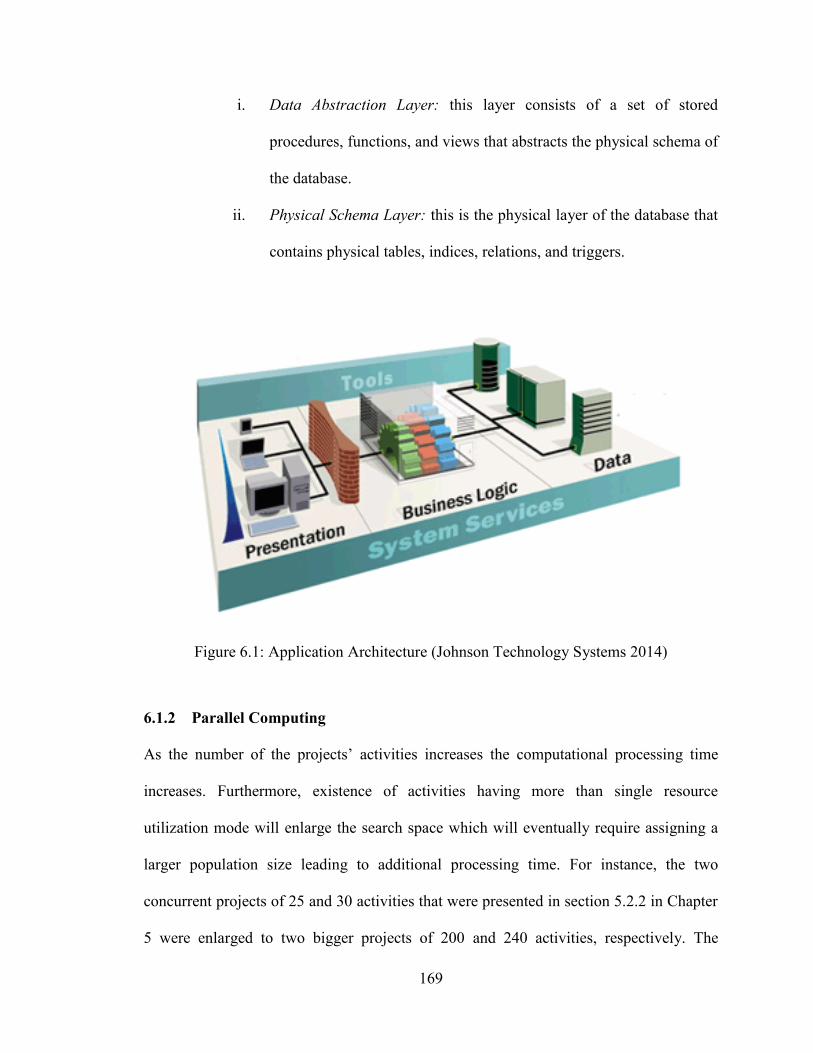
169
i. Data Abstraction Layer: this layer consists of a set of stored
procedures, functions, and views that abstracts the physical schema of
the database.
ii. Physical Schema Layer: this is the physical layer of the database that
contains physical tables, indices, relations, and triggers.
Figure 6.1: Application Architecture (Johnson Technology Systems 2014)
6.1.2 Parallel Computing
As the number of the projects’ activities increases the computational processing time
increases. Furthermore, existence of activities having more than single resource
utilization mode will enlarge the search space which will eventually require assigning a
larger population size leading to additional processing time. For instance, the two
concurrent projects of 25 and 30 activities that were presented in section 5.2.2 in Chapter
5 were enlarged to two bigger projects of 200 and 240 activities, respectively. The

170
population size and number of generations were assumed to be 1200 and 1000,
respectively. The model was run using a desktop with a quad-core processor of 3.2 GHz
speed. It took around 67 hours to complete the optimization process by reaching the
preset number of generations. Moreover, the quality of optimized solutions was not
satisfying due to the relatively small population size and number of generations defined.
In fact, the search space becomes larger as the number of activities increases together
with the number of utilization modes for each activity. Thus, a larger population size and
number of generations will be required to improve the quality of solutions leading to
additional processing time, i.e. more than 67 hours. The major portion of such high
computational time is exerted in the fitness evaluation phase.
Accordingly, the application is designed and built to execute parallel computing. The
parallelism takes place by performing parallel fitness evaluation of the multi-objectives
over multi-processors with multi-cores to support the optimization of large-scale
construction projects by reducing its processing time. As illustrated in Figure 6.2, the
application is designed to distribute its computations using the following nine cyclic
steps:
1. The message passing interface (MPI) functions are initialized to facilitate the
communication between the manager and worker processors.
2. The manager processor generates a population of solutions that represents a
number of feasible construction schedules.
3. The manager processor divides the population into sub-populations and sends
each sub-population to a multi-core worker processor.

171
4. Each multi-core worker processor further divides the sub-population into sub-
subpopulations and sends each sub-subpopulation to a core within the same
worker processor.
5. Each core within each worker processor evaluates the fitness of the multi-
objectives of each construction schedule in the sub-subpopulation.
6. Each core sends the objectives’ values to their respective worker processor.
7. Each multi-core worker processor sends the objectives’ values to the manager
processor.
8. The manager processor collects the results and performs GA operations (i.e.
selection, crossover, and mutation) to generate the next population.
9. Finally, steps 3 through 8 are repeated until total number of generations are met.
It was difficult to have an access for a supercomputing network facility to apply the
parallel computing feature described above. Thus, this feature was applied on a small
scale by running the 25-30 activity projects example using a dual-core and a quad-core
processors to check its validity. The population size and number of generations were
assumed to be 800 and 600, respectively. It took around 6 hours to solve the problem
using the dual-core processor. On the other hand, the problem was solved in around 3
hours using the quad-core processor. As a result, increasing the number of cores from two
to four resulted in a 50% reduction in the processing time. This reduction was due to the
fact that the computational effort of the total population was distributed among four cores
instead of two. Therefore, it can be expected to achieve more reduction in the processing
time if more cores and/or processors are available.
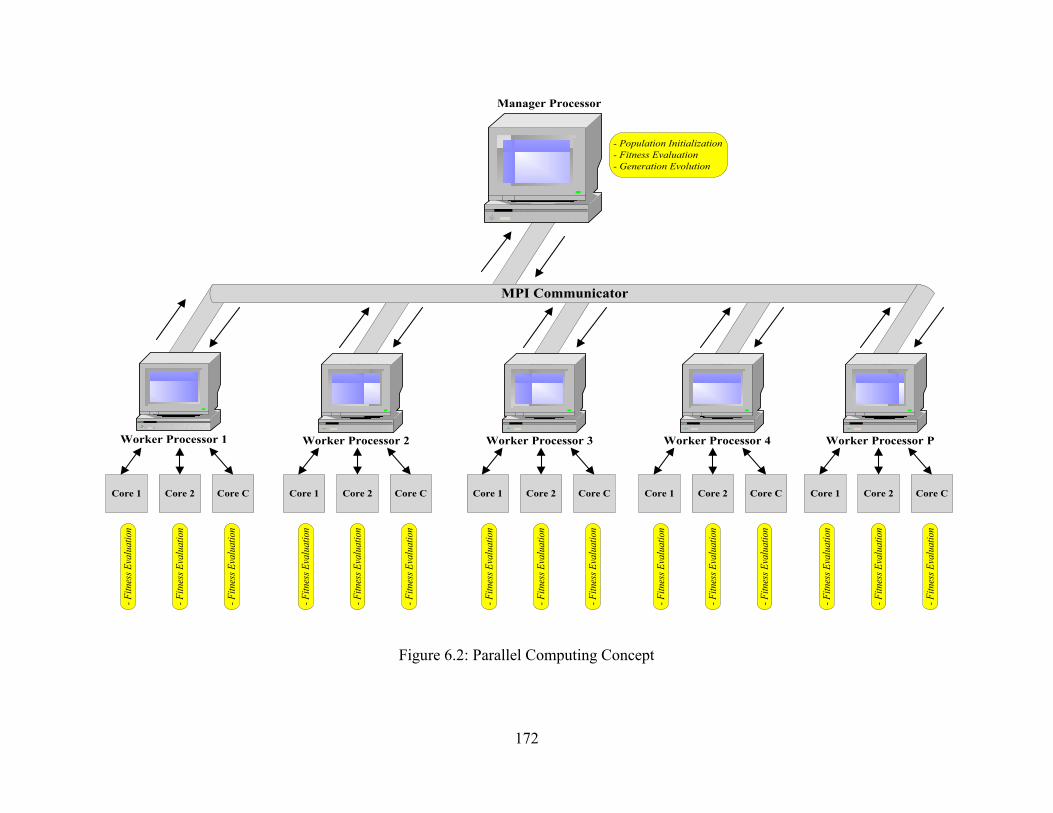
172
Worker Processor 1 Worker Processor 2 Worker Processor 4Worker Processor 3
MPI Communicator
Worker Processor P
Manager Processor
Core 1 Core 2 Core C
- F
itnes
s E
valu
ati
on
- F
itnes
s E
valu
ati
on
- F
itnes
s E
valu
ati
on
Core 1 Core 2 Core C
- F
itnes
s E
valu
ati
on
- F
itnes
s E
valu
ati
on
- F
itnes
s E
valu
ati
on
Core 1 Core 2 Core C-
Fit
nes
s E
valu
ati
on
- F
itnes
s E
valu
ati
on
- F
itnes
s E
valu
ati
on
Core 1 Core 2 Core C
- F
itnes
s E
valu
ati
on
- F
itnes
s E
valu
ati
on
- F
itnes
s E
valu
ati
on
Core 1 Core 2 Core C
- F
itnes
s E
valu
ati
on
- F
itnes
s E
valu
ati
on
- F
itnes
s E
valu
ati
on
- Population Initialization
- Fitness Evaluation
- Generation Evolution
Figure 6.2: Parallel Computing Concept

173
6.1.3 Application Requirements
To setup and run the application, the following requirements should be available:
1. Microsoft Dot Net Framework 4
2. Microsoft SQL Server 2008 (either Express or Enterprise)
3. Windows 7 as an operating system or later
6.2 MOSCOPEA DEVELOPMENT
As shown in Figure 6.3, the development of MOSCOPEA application comprises three
main units: (1) a relational database unit to facilitate the storage and retrieval of all the
input and output data; (2) a processing unit that integrates both management and multi-
objective optimization sub-units to perform all the required analysis; and (3) a GUI unit
to facilitate the input of all the projects’ data and visualize the outputs of the system. The
GUI, processing, and relational database units are equivalent to the presentation, business
logic, and data tiers, respectively as discussed earlier.
6.2.1 Relational Database Unit
The main purpose of this unit is to develop a relational database capable of storing the
necessary input data (e.g. activities description and relations, available resource
utilization modes for each activity, analysis parameters, etc.) and the produced output
data (e.g. generated optimal tradeoff among different objectives). Thus, this unit is
composed of eight main tables designed to store the following construction planning and
analysis data: (1) projects set number; (2) projects’ generic, time, financial, and
contractual data; (3) projects’ activities; (4) precedence relationships among activities; (5)
174
activities’ cost, duration, and number of resources associated with each resource
utilization mode; (6) analysis parameters; (7) optimal start time, finish time, and resource
utilization mode for each activity; and (8) optimal multi-objective tradeoffs. Figure 6.4
shows a schematic representation of these database tables and the relationships among
them using an entity relationship diagram.
The “project set” table is designed to store the number of concurrent projects set needed
to be analyzed. This table is linked using a one-to-many relationship to (1) the “projects”
table that stores each project’s time, financial, and contractual data; and (2) the “analysis
case” table which stores different analysis parameters including the GA parameters,
credit and resource constraints, and desired objectives to be optimized simultaneously.
The “projects” table is linked to the “activities” table which stores the descriptions and
IDs of all projects’ activities using a one-to-many relationship. The “activities” table is
linked using a one-to-many relationship to (1) the “activities dependencies” table that
stores the predecessors of each activity; and (2) the “activities resource utilization mode”
table that stores the duration, cost, and number of resources of each activity associated
with each resource utilization mode. The “activities” table is also linked using a many-to-
many relationship to the “optimal activity schedules” table that is designed to store the
identified optimal schedule for each activity, including its (1) optimal resource utilization
mode; (2) optimal duration and cost; and (3) optimal start and finish times. Finally, the
“optimal activity schedules” table is linked using a one-to-one relationship to the
“optimal tradeoffs” table which stores the identified set of optimal tradeoffs among the
projects’ selected objectives to be optimized simultaneously. The main purpose of the

175
relationships linking the tables in the relational database unit (one to one, one to many, or
many to many) is to ensure the integrity of the data stored in the database during the input
and output phases. For example, the relationship linking the “activities” table to the
“activities resource utilization mode” table is specified to be a one-to-many relationship
to ensure that each entered resource utilization mode is assigned to a single and unique
activity in the project and that the deletion of that activity will automatically lead to the
deletion of all its assigned resource utilization modes.
6.2.2 Processing Unit
The processing unit acts as the core unit of MOSCOPEA which coordinates all the data
in order to perform all the required analysis. As shown in Figure 6.3, the processing unit
is divided into two sub-units: (1) management sub-unit; and (2) multi-objective
optimization sub-unit. The “management” sub-unit comprises the scheduling, cash flow,
and resource models which are used to determine the multi-objectives (i.e. total duration,
total cost, financing cost, required credit, profit, resource fluctuation and peak demand)
values as explained earlier in Chapter 3. On the other hand, the “multi-objective
optimization” sub-unit performs the three main phases of the NSGA-II technique (i.e.
population initialization, fitness evaluation, and generation evolution) to obtain optimal
tradeoffs between the multi-objectives as discussed earlier in Chapter 4. Both sub-units
interacts together to perform all the required analysis using the data stored in the
relational database unit.

176
GRAPHICAL USER INTERFACE UNIT
Input Phase
Input Number
of Projects
Input
Projects’
Parameters
Input
Activities’
Parameters
Input Resource
Utilization
Modes
Input
Analysis
Parameters
Output Phase
Optimal
TradeoffsBar Chart
Activities
Details
Net Cash
Flow
Diagram
Resource
Profile
RELATIONAL DATABASE UNIT
Proj
ects
Set
Ta
ble
Act
ivit
ies
Tabl
e
Proj
ects
Ta
ble
Ana
lysi
s C
ase
Tabl
e
Act
ivit
ies
Dep
ende
ncie
s Ta
ble
Act
ivit
ies
Res
ourc
e U
tiliz
atio
n M
ode
Opt
imal
Tr
adeo
ffs
Tabl
e
Opt
imal
A
ctiv
ity
Sche
dule
s Ta
ble
PROCESSING UNIT
MANAGEMENT SUB-UNIT
Scheduling Model
Resource Model
Cash Flow Model
MULTI-OBJECTIVE
OPTIMIZATION SUB-UNIT
Population
Initialization
Fitness Evaluation
Generation Evolution
Export Outputs
Figure 6.3: MOSCOPEA Development Framework
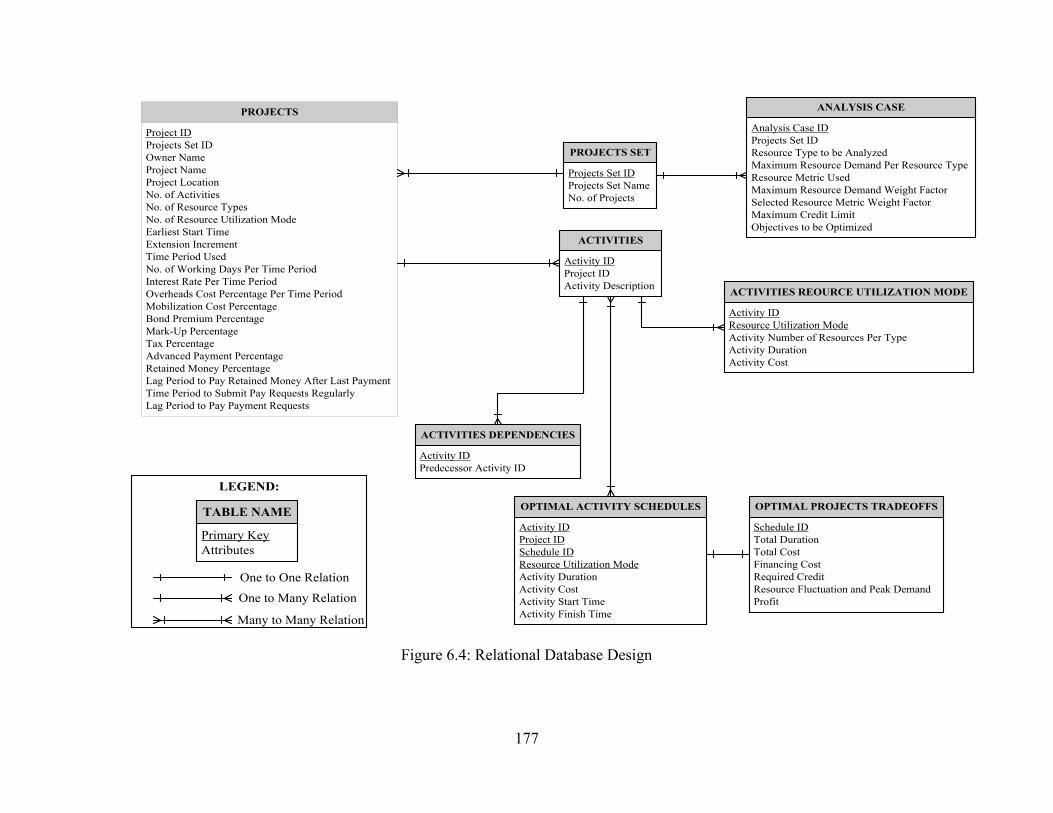
177
PROJECTS
Project ID
Projects Set ID
Owner Name
Project Name
Project Location
No. of Activities
No. of Resource Types
No. of Resource Utilization Mode
Earliest Start Time
Extension Increment
Time Period Used
No. of Working Days Per Time Period
Interest Rate Per Time Period
Overheads Cost Percentage Per Time Period
Mobilization Cost Percentage
Bond Premium Percentage
Mark-Up Percentage
Tax Percentage
Advanced Payment Percentage
Retained Money Percentage
Lag Period to Pay Retained Money After Last Payment
Time Period to Submit Pay Requests Regularly
Lag Period to Pay Payment Requests
PROJECTS SET
Projects Set ID
Projects Set Name
No. of Projects
ACTIVITIES
Activity ID
Project ID
Activity Description
ACTIVITIES DEPENDENCIES
Activity ID
Predecessor Activity ID
ACTIVITIES REOURCE UTILIZATION MODE
Activity ID
Resource Utilization Mode
Activity Number of Resources Per Type
Activity Duration
Activity Cost
ANALYSIS CASE
Analysis Case ID
Projects Set ID
Resource Type to be Analyzed
Maximum Resource Demand Per Resource Type
Resource Metric Used
Maximum Resource Demand Weight Factor
Selected Resource Metric Weight Factor
Maximum Credit Limit
Objectives to be Optimized
OPTIMAL ACTIVITY SCHEDULES
Activity ID
Project ID
Schedule ID
Resource Utilization Mode
Activity Duration
Activity Cost
Activity Start Time
Activity Finish Time
OPTIMAL PROJECTS TRADEOFFS
Schedule ID
Total Duration
Total Cost
Financing Cost
Required Credit
Resource Fluctuation and Peak Demand
Profit
TABLE NAME
Primary Key
Attributes
One to One Relation
One to Many Relation
Many to Many Relation
LEGEND:
Figure 6.4: Relational Database Design

178
6.2.3 Graphical User Interface (GUI) Unit
The GUI unit is implemented in MOSCOPEA to facilitate the input of all the necessary
construction scheduling data and the output of the generated optimal schedules. The unit
is designed to implement the necessary interface functions in two main phases: (1) an
input phase that facilitates the input of the projects’ data, activities’ data, resource
utilization modes, and analysis parameters; and (2) an output phase that allows the end
user to visualize the optimal activity schedules and the optimal tradeoffs among the
desired multi-objectives obtained by MOSCOPEA. Figure 6.5 shows the welcome
window of MOSCOPEA. The detailed procedure of implementing the GUI of
MOSCOPEA is discussed in the next section.
Figure 6.5: MOSCOPEA Welcome Window

179
6.3 MOSCOPEA GUI IMPLEMENTATION PROCEDURE
The example of the nine-activity single project adopted from Leu and Yang (1999) is
used herein to illustrate for the end user the procedure of implementing the GUI of
MOSCOPEA.
6.3.1 Input Phase
The GUI input phase of MOSCOPEA comprises two main windows named A and B.
Window (A) includes the activities’ data, projects’ data, and resource utilization modes.
While, window (B) includes all the necessary analysis parameters. Window (A) is
divided into eight panels (Figure 6.6) and window (B) is divided into two panels (Figure
6.7).
6.3.1.1 Window (A)
Step 1: Create New Solution
First the user is prompted using the “file” icon to either open an existing saved solution or
to create a new solution as shown in Figure 6.8. Consequently, a pop-up window appear
asking the user to input the solution name, number of projects, number of resource types,
and number of resource utilization mode for each activity as shown in Figure 6.8. It is
worth to mention that the number of resource utilization modes entered will be initially
considered equal for all the activities. However, the user can delete or add later the
number of modes for each activity based on the problem being solved.
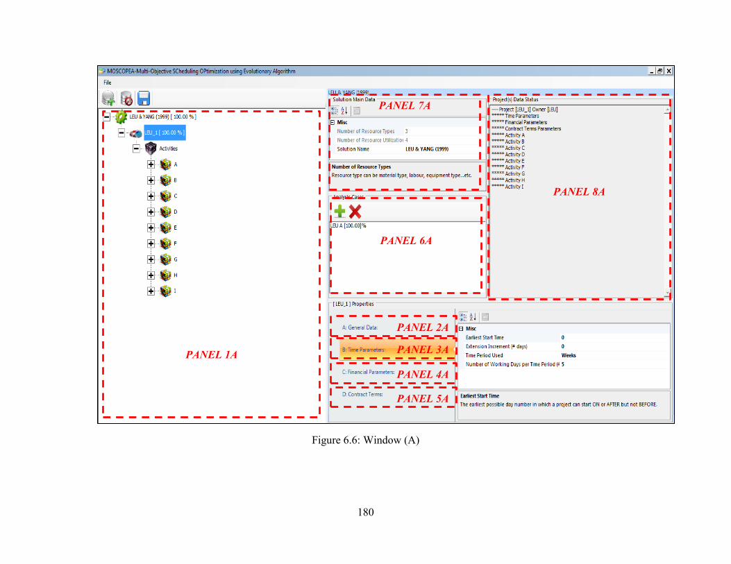
180
Figure 6.6: Window (A)
PANEL 1A
PANEL 2A
PANEL 3A
PANEL 4A
PANEL 5A
PANEL 6A
PANEL 7A
PANEL 8A

181
Figure 6.7: Window (B)
PANEL 1B
PANEL 2B

182
Figure 6.8: Create New Solution
Step 2: Identify Activities and Precedence Relationship
The user then has to identify all the activities and their precedence relationship in panel
1A as shown in Figure 6.9.
Step 3: Identify Resource Utilization Modes
Having all the activities identified, the user is then prompted to identify the duration,
cost, and number of daily resources for each activity and its associated resource
utilization mode in panel 1A as shown in Figure 6.10. Figure 6.11 shows a sample for
one of the activities after all its necessary data are identified.

183
Figure 6.9: Identify Activities and Precedence Relationship
Figure 6.10: Identify Resource Utilization Modes

184
Figure 6.11: Full Identified Data for an Activity Sample
Step 4: Identify Project’s Data
This step involves identifying the project’s general data (panel 2A), time parameters
(panel 3A), financial parameters (panel 4A), and contract terms (panel 5A) as shown in
Figures 6.12 to 6.15. In case more than one project are considered, those four types of
data are to be identified for each project individually.
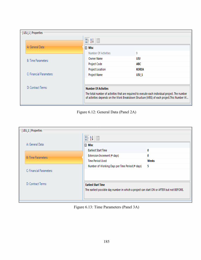
185
Figure 6.12: General Data (Panel 2A)
Figure 6.13: Time Parameters (Panel 3A)

186
Figure 6.14: Financial Parameters (Panel 4A)
Figure 6.15: Contract Terms (Panel 5A)
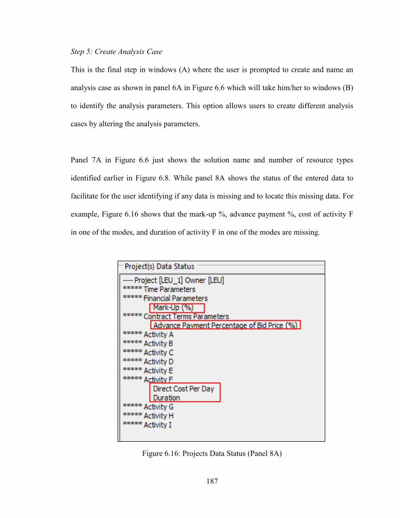
187
Step 5: Create Analysis Case
This is the final step in windows (A) where the user is prompted to create and name an
analysis case as shown in panel 6A in Figure 6.6 which will take him/her to windows (B)
to identify the analysis parameters. This option allows users to create different analysis
cases by altering the analysis parameters.
Panel 7A in Figure 6.6 just shows the solution name and number of resource types
identified earlier in Figure 6.8. While panel 8A shows the status of the entered data to
facilitate for the user identifying if any data is missing and to locate this missing data. For
example, Figure 6.16 shows that the mark-up %, advance payment %, cost of activity F
in one of the modes, and duration of activity F in one of the modes are missing.
Figure 6.16: Projects Data Status (Panel 8A)

188
6.3.1.2 Window (B)
As shown in Figure 6.7, this window involves inputting all the different analysis
parameters. In panel 1B, the user has the flexibility to select the resource metric to be
used (i.e. RID or RRH) and to identify the MRD and selected resource metric weight
factor. This is followed by identifying the maximum credit limit. In case no credit limit
constraint is required, then the user can just input a very large value. After that, all the
GA parameters are to be identified including the population size, number of generations,
crossover probability, and mutation probability. Finally, the user has the flexibility to
select one or more objective(s) to be optimized simultaneously by assigning for each
objective a “true” or “false” value should the objective be selected or not, respectively. In
panel 2B, the user has the flexibility to select one or more resource type to be analyzed –
in case of multi-resources – and to identify the maximum daily resource limit for each
resource type. Again, in case no resource limit constraint is required, then the user can
just input a very large value. Finally, the user has to click on the optimize button and
assign a folder on his/her desktop in which all the outputs will be exported as shown in
Figure 6.17. Consequently, an analysis progress bar will appear as shown in Figure 6.18.
Figure 6.17: Optimize and Assign Output Folder
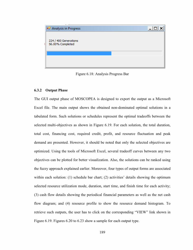
189
Figure 6.18: Analysis Progress Bar
6.3.2 Output Phase
The GUI output phase of MOSCOPEA is designed to export the output as a Microsoft
Excel file. The main output shows the obtained non-dominated optimal solutions in a
tabulated form. Such solutions or schedules represent the optimal tradeoffs between the
selected multi-objectives as shown in Figure 6.19. For each solution, the total duration,
total cost, financing cost, required credit, profit, and resource fluctuation and peak
demand are presented. However, it should be noted that only the selected objectives are
optimized. Using the tools of Microsoft Excel, several tradeoff curves between any two
objectives can be plotted for better visualization. Also, the solutions can be ranked using
the fuzzy approach explained earlier. Moreover, four types of output forms are associated
within each solution: (1) schedule bar chart; (2) activities’ details showing the optimum
selected resource utilization mode, duration, start time, and finish time for each activity;
(3) cash flow details showing the periodical financial parameters as well as the net cash
flow diagram; and (4) resource profile to show the resource demand histogram. To
retrieve such outputs, the user has to click on the corresponding “VIEW” link shown in
Figure 6.19. Figures 6.20 to 6.23 show a sample for each output type.

190
Figure 6.19: Optimal Tradeoffs Output

191
Figure 6.20: Bar Chart Output
Figure 6.21: Activities’ Details Output

192
Figure 6.22: Cash Flow Details Output
Figure 6.23: Resource Profile Output

193
CHAPTER 7: CONCLUSIONS AND RECOMMENDATIONS
7.1 SUMMARY AND CONCLUSIONS
Surveys of construction practitioners point to financial and budgetary factors as the
leading causes of construction business failures. Such leading causes are mainly due to
inefficient control and management of contractor’s cash flow. This inefficiency is due to
the fact that contractors mainly deal with the project scheduling and financing as two
independent functions of construction project management. The absence of the required
linkage between those two functions resulted in devising non-executable schedules which
lead to a high volume of project failure due to finance deficit. Thus, controlling and
regulating the movement of the cash is necessary for the success of the construction
projects. According to the literature review carried in this research, there was a lack of
research that considers integrating both resource leveling and allocation simultaneously
with the finance-based scheduling concept. Considering those two aspects together have a
significant impact on many areas of project management including time, cost, resource,
and risk. Moreover, few researches solved the finance-based scheduling problem
considering the contractor’s entire portfolio rather than single project. Multiple
concurrent projects involves sharing and competing for limited resources such as funds,
equipment, manpower and other resources among different projects, which increases the
complexity of the scheduling process.
As a result, it was motivated in this research to present the development of a novel multi-
objective scheduling optimization model for multiple construction projects. The novelty
194
arises throughout considering both financial and resource aspects under a single platform.
Such aspects were considered by integrating the concept of finance-based scheduling
together with resource leveling and allocation for concurrent multiple projects. The
model enables construction companies in solving the problems of how to prioritize the
projects with resource conflicts, how to reasonably allocate the limited resources among
multiple projects to meet the resource requirements of different projects, and to optimize
all the projects’ multi-objectives under cash limits. The multi-objectives included in this
optimization model were the total duration, total cost, financing cost, required credit,
profit, resource fluctuations and peak demand.
Three main management models were developed to adapt for multiple construction
projects, namely: scheduling, cash flow, and resource model. The main aim of these
models is to evaluate the projects’ different multi-objectives values. The scheduling
model establishes optimal/near optimal schedules for multiple construction projects to
determine the projects’ total duration and identify the activities’ start and finish times.
The cash flow model determines the total cost, financing cost, required credit, and profit
of multiple projects based on the schedules obtained from the scheduling model. Finally,
the resource model determines the resource fluctuations and daily maximum resource
demand for multiple projects based also on the schedules obtained from the scheduling
model.
Consequently, a complete optimization model formulation was established to identify the
model’s decision variables, formulate the optimization objectives, and model the

195
optimization constraints. The decision variables comprised both the start times and
resource utilization modes of the projects’ activities. On the other hand, the model was
formulated under the constraints of preserving the logical relationship between activities
while keeping the maximum required credit and resource demand below pre-defined
limits.
Accordingly, a multi-objective scheduling optimization model was developed for
multiple construction projects using multi-mode activities with multi-resources. The
developed model was linked with the three management models (scheduling, cash flow,
and resource) to search for schedules that optimize the projects’ desired objectives using
the NSGA-II technique. The model performed the genetic algorithm operations in three
main phases: (1) population initialization; (2) fitness evaluation; and (3) generation
evolution.
The model was tested to solve a time/cost tradeoff problem, integrated time/cost tradeoff
and resource allocation problem, and a finance-based scheduling problem retrieved from
literature. The testing results were compared with the previous ones and the model
proved its robustness in solving such problems. Moreover, the model was applied on
three case studies to demonstrate its capabilities to solve integrated resource leveling,
resource allocation, and finance-based scheduling problems for single and multiple
projects under unconstrained and constrained credit and resource limits.
196
Finally, an automated tool named MOSCOPEA (Multi-Objective SCheduing
OPtimization using Evolutionary Algorithm) was built with a friendly graphical user
interface to facilitate in selecting the optimum/near optimum start times and resource
utilization modes of activities that optimizes the projects’ desired objectives. The tool
was designed and built to execute parallel computing by performing parallel fitness
evaluation of the multi-objectives over multi-processors with multi-cores to support the
optimization of large-scale construction projects by reducing its processing time.
7.2 RESEARCH CONTRIBUTIONS
The main contributions of this research can be summarized as follows:
1. Development of a strategy or methodology to integrate CPM schedules with their
associated cash flows and resource profiles for multiple construction projects.
2. Development of a multi-objective scheduling optimization model for multiple
construction projects considering both financial and resource aspects. Such model
enables planners to devise optimal/near optimal schedules for multiple projects
that simultaneously: (a) satisfies certain credit and resource limits; (b) minimize
undesirable resource fluctuations, i.e. increase the efficiency of resource
utilization; and (c) maximize contractors’ profit.
3. Adding flexibility to the developed model in selecting the desired set of objectives
to be optimized together. In other words, different tradeoffs between different set
of selected objectives can be obtained from the model. The merit of this flexibility
is in allowing contractors to examine the impact of one or more objectives over
the other on the projects’ schedule. Thus, the model can solve individually the
197
time/cost tradeoff, resource leveling, resource allocation, or finance-based
scheduling problems. Alternatively, integration of such problems can be also
solved.
4. Designing and building an automated tool (MOSCOPEA) with a friendly
graphical user interface that incorporates the above points under a single platform
to facilitate for practitioners the scheduling optimization process in the
construction industry.
7.3 RESEARCH LIMITATIONS
The research has some limitations which can be summarized as follows:
1. The developed model considers only the finish-to-start precedence relationship
between the projects’ activities.
2. The scheduling model does not allow for activities’ interruption or splitting
caused by different parties.
3. The cash flow model applies only for unit-price type contracts. In addition, it does
not consider for projects’ activities that are executed by sub-contractors.
4. The cash flow model does not consider the cost of resource idle days as well as
the early completion bonus.
5. The developed automated tool requires the user to manually enter the activities’
time, cost, and resource data one by one which consumes more time than just
simply importing such data in a tabulated form.
6. In the absence of multi-processors with multi-cores, the automated tool may not
be suitable to solve large-scale projects due to high computational time.

198
7.4 RECOMMENDATIONS FOR FUTURE WORK
The current research study has been able to accomplish its main objectives. Yet, several
points are recommended to enhance and extend the current research for future work.
7.4.1 Current Research Recommended Enhancements
The model should cover all other types of precedence relationships (i.e. finish-to-
finish, start-to-start, and start-to-finish) and should consider also the time lag
between activities. Taking such relationships into consideration is essential to
develop more practical schedules by overlapping the activities of a network to
accelerate the execution of a project.
The cash flow model can be modified to account for the charges of the unused
credit limit. The interest rate of the unused credit fee is lower than the interest rate
on actual negative balances because the bank can likely lend the unused funds to
another borrower. Taking this into consideration can improve (minimize) the
financing costs for the contractor.
The optimization model can consider allocating a priority weight for each
concurrent project to assign efficiently the available resources and cash among
different projects.
Using a certain metaheuristic technique to efficiently solve a specific problem,
may not adequately solve other optimization problems. Similarly, a problem can
be solved differently by various algorithms. As a result, other promising meta-
heuristics techniques such as ant colony or particle swarm optimization can be
experimented to solve the currently developed model. Such techniques can be
199
compared with the used NSGA-II technique to select the most suitable one based
on the quality of the results as well as the processing time.
In reality, many factors exist during construction that may affect the cash flow
including time delays, cost overruns, unconfirmed earned values, change orders,
and changes of cost plan elements. Thus, for more practical schedules, activities’
interruption or splitting caused by different parties can be considered. Moreover,
uncertainties in the activities’ duration and cost can be considered while
scheduling the projects.
7.4.2 Current Research Recommended Extensions
The cash flow model of this research applies only for unit-price type contracts.
Thus, the cash flow model structure can be adjusted to suit other different types of
construction contracts. This can be done by studying and applying the different
contracts’ methods of payment as well as the timing of payment which can highly
affect the project schedule.
Sometimes contractors may face problems of being timely paid by the owner. A
failure of the contractor getting regular and timely payment could result in project
delay, reduced profitability, and in the extreme case, the company may go into
liquidation. Therefore, the model should be further experimented to address
owner’s late payment. This can be done by altering the “lag to pay payment
requests” parameter in the current model to create “what-if” scenarios. Thus,
several late payment scenarios can be established, studied, and compared to
account for delays in owner’s payment.

200
Heavy construction projects such as highways, tunnels, and bridges usually age
and deteriorate at a fast rate requiring immediate rehabilitation efforts to enhance
their quality. Therefore, other objectives such as the “construction method
quality” can be added to be optimized together with the identified multi-
objectives.

201
REFERENCES
Abido, M.A., and Elazouni, A.M. (2010). “Precedence-Preserving GAs Operators for
Scheduling Problems with Activities’ Start Times Encoding”, Journal of
Computing in Civil Engineering, ASCE, Vol. 24, No. 4, pp. 345-356.
Abido, M.A., and Elazouni, A.M. (2011). “Multiobjective Evolutionary Finance-Based
Scheduling: Entire Projects’ Portfolio”, Journal of Computing in Civil
Engineering, ASCE, Vol. 25, No. 1, pp. 85-97.
Afshar, A., and Fathi, H. (2009). “Fuzzy Multi-objective Optimization of Finance-Based
Scheduling for Construction Projects with Uncertainties in Cost”, Engineering
Optimization, Vol. 41, No. 11, pp. 1063-1080.
Ahmed. M., Elazouni, A.M., and Zayed, T. (2011). “Assessment of activities criticality
related to cash flow parameters”, Proceedings of Canadian Society of Civil
Engineering (CSCE) / Construction Research Congress (CRC), Ottawa, Ontario,
June 14 - 17.
Ahuja, H. (1976). “Construction Performance Control by Networks”, Wiley, NY, USA.
Alcaraz, J. and Maroto, C. (2001). “A Robust Genetic Algorithm for Resource Allocation
in Project Scheduling”, Annals of Operations Research, Vol. 102, No. 1, pp. 83-
109.
Alghazi, A., Elazouni, A., and Selim, S. (2013). “Improved Genetic Algorithm for
Finance-Based Scheduling”, Journal of Computing in Civil Engineering, Vol. 27,
No. 4, pp. 379-394.

202
Ali, M.M., and Elazouni, A.M. (2009). “Finance-Based CPM/LOB Scheduling of
Projects with Repetitive Non-serial Activities”, Construction Management and
Economics, Vol. 27, No. 9, pp. 839-856.
Allam, S.I.G. (1988). “Multi-project Scheduling: A New Categorization for Heuristic
Scheduling Rules in Construction Scheduling Problems”, Construction
Management and Economics, Vol. 6, No. 2, pp. 93-115.
Antill, J.M., and Woodhead, R.W. (1982). “Critical Path Methods in Construction
Practice”, John Wiley, 3rd
Edition, NY, USA.
April, J., Glover, F., Kelly, J.P., and Laguna, M. (2003). “Practical Introduction to
Simulation Optimization”, Simulation Conference 2003, Proceedings of the 2003
Winter, IEEE, CO, USA, pp. 71-78.
Arditi, D., Koksal, A., and Kale, S. (2000). “Business Failures in the Construction
Industry”, Engineering Construction and Architectural Management, Vol. 7, No.
2, pp. 120-132.
Au, T., and Hendrickson, C. (1986). “Profit Measures for Construction Projects”, Journal
of Construction Engineering and Management, ASCE, Vol. 112, No. 2, pp. 273-
286.
Blazewicz, J., Lenstra J.K. and Rinnooy A.H.G. (1983). “Scheduling Projects to
Resource Constraints: Classification and Complexity”, Discrete Applied
Mathematics, Vol. 5, pp. 11-24.
Boussabaine, A.H., and Kaka, A.P. (1998). “A Neural Networks Approach for Cost Flow
Forecasting”, Construction Management & Economics, Vol. 16, No. 4, pp. 471-
479.

203
Burgess, A.R., and Killebrew, J.B. (1962). “Variation in Activity Level on a Cyclical
Arrow Diagram”, Journal of Industrial Engineering, Vol. 13, No. 2, pp. 76-83.
Burns, S.A., Liu, L., and Feng, C.W. (1996). “The LP/IP Hybrid Method for Construction
Time-Cost Trade-Off Analysis”, Construction Management and Economics, Vol.
14, No. 3, pp. 265-276.
Chan, W., Chua, K., and Kannan, G. (1996). “Construction Resource Scheduling with
Genetic Algorithms”, Journal of Construction Engineering and Management,
ASCE, Vol. 122, No. 2, pp. 125-132.
Chassiakos, A.P., and Sakellaropoulos, S.P. (2005). “Time-Cost Optimization of
Construction Projects with Generalized Activity Constraints”, Journal of
Construction Engineering and Management, ASCE, Vol. 131, No. 10, pp. 1115-
1124.
Chen, P.H., and Shahandashti, S.M. (2007). “Simulated Annealing Algorithm for
Optimizing Multi-project Linear Scheduling with Multiple Resource Constraints”,
The 24th International Symposium on Automation and Robotics in Construction.
ISARC 2007, Madras, India, pp. 429-434.
Chen, P.H., and Weng, H. (2009). “A Two-phase GA Model for Resource-Constrained
Project Scheduling”, Automation in Construction, Vol. 18, No. 4, pp. 485-498.
Chiu, H.N., and Tsai, D.M. (2002). “An Efficient Search Procedure for the Resource-
Constrained Multi-project Scheduling Problem with Discounted Cash Flows”,
Construction Management and Economics, Vol. 20, No. 1, pp. 55-66.
Coello, C.A. (2000). “An Updated Survey of GA-based Multiobjective Optimization
Techniques”, ACM Computing Surveys, Vol. 32, No. 2, pp. 109-143.
204
Coello, C.C., Pulido, G.T., and Montes, E.M. (2005). “Current and Future Research
Trends in Evolutionary Multiobjective Optimization”, Information Processing
with Evolutionary Algorithms, Springer London, pp. 213-231.
Davis, E.W. (1973). “Project Scheduling Under Resource Constraints—Historical
Review and Categorization of Procedures”, AIIE Transactions, Vol. 5, No. 4, pp.
297-313.
Davis, E.W., and Patterson, J.H. (1975). “A Comparison of Heuristic and Optimum
Solutions in Resource-Constrained Project Scheduling”, Management science,
Vol. 21, No. 8, pp. 944-955.
Dawood, N., and, Sriprasert, E. (2006). “Construction Scheduling Using Multi-constraint
and Genetic Algorithms Approach”, Construction Management and Economics,
Vol. 24, No. 1, pp. 19-30.
De, P., Dunne, E.J., Ghosh, J.B., and Wells, C.E. (1995). “The Discrete Time-Cost
Tradeoff Problem Revisited”, European Journal of Operational Research, Vol. 81,
No. 2, pp. 225-238.
Deb, K. (2001). “Multi-Objective Optimization Using Evolutionary Algorithms”, Wiley,
NY, USA.
Deb, K., Pratap, A., Agarwal, S., and Meyarivan, T. (2002). “A Fast and Elitist
Multiobjective Genetic Algorithm: NSGA-II”. IEEE Transactions on
Evolutionary Computation, Vol. 6, No. 2, pp. 182-197.
Dhillon, J.S., Parti, S.C., and Kothari, D.P. (1993). “Stochastic Economic Emission Load
Dispatch”, Electric Power Systems Research, Vol. 26, No. 3, pp. 179-186.

205
Dumond, J., and Mabert, V.A. (1988). “Evaluating Project Scheduling and Due Date
Assignment Procedures: An Experimental Analysis”, Management Science, Vol.
34, No. 1, pp. 101-118.
Easa, S. (1989). “Resource Leveling in Construction by Optimization”, Journal of
Construction Engineering and Management, ASCE, Vol. 115, No. 2, pp. 302-316.
Elazouni, A.M. (2009). “Heuristic Method for Multi-project Finance-Based Scheduling”,
Construction Management and Economics, Vol. 27, No. 2, pp. 199-211.
Elazouni, A., and Abido, M.A. (2014). “Enhanced Trade-Off of Construction Projects:
Finance-Resource-Profit”, Journal of Construction Engineering and Management,
ASCE, Vol. 140. No. 9.
Elazouni, A., and Abido, M. (2011). “Multiobjective Evolutionary Finance-Based
Scheduling: Individual Projects within a Portfolio”, Automation in Construction,
Vol. 20, No. 7, pp. 755-766.
Elazouni, A.M., and Gab-Allah, A.A. (2004). “Finance-Based Scheduling of
Construction Projects Using Integer Programming”, Journal of Construction
Engineering and Management, ASCE, Vol. 130, No. 1, pp. 15-24.
Elazouni, A.M., and Metwally, F.G. (2005). “Finance-Based Scheduling: Tool to
Maximize Project Profit Using Improved Genetic Algorithms”, Journal of
Construction Engineering and Management, ASCE, Vol. 131, No. 4, pp. 400-412.
Elazouni, A.M., and Metwally, F.G. (2007). “Expanding Finance-Based Scheduling to
Devise Overall-Optimized Project Schedules”, Journal of Construction
Engineering and Management, ASCE, Vol. 133, No. 1, pp. 86-90.

206
Elmaghraby, S.E. (1993). “Resource Allocation Via Dynamic Programming in Activity
Networks”, European Journal of Operational Research, Vol. 64, No. 2, pp. 199-
215.
El-Rayes, K., and Jun, D.H. (2009). “Optimizing Resource Leveling in Construction
Projects”, Journal of Construction Engineering and Management, ASCE, Vol.
135, No. 11, pp. 1172-1180.
El-Rayes, K., and Kandil, A. (2005). “Time-Cost-Quality Trade-Off Analysis for
Highway Construction”, Journal of Construction Engineering and Management,
ASCE, Vol. 131, No. 4, pp. 477-486.
Esfahan, N.R. (2011). “Project Schedule Compression Considering Multi-objective
Decision Environment”, M.Sc Thesis, Building Construction Department,
Concordia University, Montreal, Quebec, Canada.
Eshtehardian, E., Afshar, A., and Abbasnia, R. (2008). “Time-Cost Optimization: Using
GA and Fuzzy Sets Theory for Uncertainties in Cost”, Construction Management
and Economics, Vol. 26, No. 7, pp. 679-691.
Fatemi-Ghomi, S.M.T., and Ashjari, B. (2002). “A Simulation Model for Multi-project
Resource Allocation”, International Journal of Project Management, Vol. 20, No.
2, pp. 127-130.
Fathi, H., and Afshar, A. (2010). “GA-Based Multi-objective Optimization of Finance-
Based Construction Project Scheduling”, KSCE Journal of Civil Engineering,
Vol. 14, No. 5, pp. 627-638.
Fendley, L.G. (1968). “Towards the Development of a Complete Multiproject Scheduling
System”, Journal of Industrial Engineering, Vol. 19, No. 10, pp. 505-515.

207
Feng, C.W., Liu, L., and Burns, S.A. (1997). “Using Genetic Algorithms to Solve
Construction Time-Cost Trade-Off Problems”, Journal of Computing in Civil
Engineering, ASCE, Vol. 11, No. 3, pp. 184-189.
Fondahl, J.M. (1961). “A Non-Computer Approach to the Critical Path Method for the
Construction Industry”, Technical Report, No. 9, Construction Institute,
Department of Civil Engineering, Stanford University.
Fonseca, C.M., and Fleming, P.J. (1993). “Multiobjective Genetic Algorithms”, IEE
Colloquium on Genetic Algorithms for Control Systems Engineering, 28 May,
London, UK.
Gavish, B., and Pirkul, H. (1991). “Algorithms for Multi-resource Generalized
Assignment Problem”, Management Science, Vol. 37, No. 6, pp. 695-713.
Goldberg, D.E. (1989). “Genetic Algorithms in Search, Optimization, and Machine
Learning”, Addison-Wesley, Reading, Massachusetts, USA.
Goncalves, J.F., Mendes, J.J., and Resende, M.G. (2008). “A Genetic Algorithm for the
Resource Constrained Multi-project Scheduling Problem”, European Journal of
Operational Research, Vol. 189, No. 3, pp. 1171-1190.
Gould, F. E. (2005). “Managing the Construction Process: Estimating, Scheduling, and
Project Control”, Pearson Education, Inc., Upper Saddle River, NJ, USA.
Guo, Y., Li, N., and Ye, T. (2009). “Multiple Resources Leveling in Multiple Projects
Scheduling Problem Using Particle Swarm Optimization”, Natural Computation,
ICNC'09, Fifth International Conference, IEEE, Tianjin, China, pp. 260-264.
Hajela, P., and Lin, C.Y. (1992). “Genetic Search Strategies in Multicriterion Optimal
Design”, Structural and Multidisciplinary Optimization, Vol. 4, No. 2, pp. 99-107.
208
Harris, R.B. (1978). “Precedence and Arrow Networking Techniques for Construction”,
Wiley, NY, USA.
Hartmann, S. (2001). “Project Scheduling with Multiple Modes: A Genetic Algorithm”,
Annals of Operations Research, Vol. 102, No. 1-4, pp. 111-135.
Hegazy, T. (1999a). “Optimization of Resource Allocation and Leveling Using Genetic
Algorithms”, Journal of Construction Engineering and Management, ASCE, Vol.
125, No. 3, pp. 167-175.
Hegazy, T. (1999b). “Optimization of Construction Time-Cost Trade-off Analysis Using
Genetic Algorithms”, Canadian Journal of Civil Engineering, Vol. 26, No. 6, pp.
685-697.
Hegazy, T. (2002). “Computer-Based Construction Project Management”, Prentice-Hall
Inc., Englewood Cliffs, NJ, USA.
Hegazy, T., and El-Zamzamy, H. (1998). “Project Management Software that Meet the
Challenge”, Cost Engineering Journal, AACE, Vol. 4, No. 5, pp. 25-33.
Hegazy, T., and Kassab, M. (2003). “Resource Optimization Using Combined Simulation
and Genetic Algorithms”, Journal of Construction Engineering and Management,
ASCE, Vol. 129, No. 6, pp. 698-705.
Hegazy, T., and Menesi, W. (2012). “Heuristic Method for Satisfying both Deadlines and
Resource Constraints”, Journal of Construction Engineering and Management,
ASCE, Vol. 138, No. 6, pp. 688-696.
Hendrickson, C., and Au, T. (1989). “Project Management for Construction”, Prentice-
Hall Inc., Englewood Cliffs, NJ, USA.
209
Herstein, M.L. (2009). “Incorporating Environmental Impacts into Multi-Objective
Optimization of Water Distribution Systems”, M.Sc Thesis, Department of Civil
Engineering, Queen’s University, Kingston, Ontario, Canada.
Hyari, K., and El-Rayes, K. (2006). “Optimal Planning and Scheduling for Repetitive
Construction Projects”, Journal of Management in Engineering, ASCE, Vol. 22,
No. 1, pp. 11-19.
Johnson, R. (1992). “Resource Constrained Scheduling Capabilities of Commercial
Project Management Software”, Project Management Journal, Vol. 22, No. 4, pp.
39-43.
Johnson Technology Systems, Inc. (2014). “Platforms and Technologies”,
<http://jtsusa.com/about/platforms-technologies/>, (November 2014).
Joshi, K., and Jain, K. (2012). “A Modified Genetic Algorithm for Resource Constrained
Project Scheduling”, International Journal of Computer Applications, Vol. 57, No.
3, pp. 41-45.
Kaka, A.P., and Price, A.D.F. (1993). “Modelling Standard Cost Commitment Curves for
Contractors' Cash Flow Forecasting”, Construction Management and
Economics, Vol. 11, No. 4, pp. 271-283.
Kanagasabapathi, B., and Ananthanarayanan, K. (2005). “A Simulation Model for
Resource Constrained Scheduling of Multiple Projects”, Proceedings of the 21st
Annual ARCOM Conference, University of London, UK, pp. 823-831.
Kandil, A., and El-Rayes, K. (2006). “Parallel Genetic Algorithms for Optimizing
Resource Utilization in Large-Scale Construction Projects”, Journal of
Construction Engineering and Management, ASCE, Vol. 132, No. 5, pp. 491-498.

210
Kangari, R. (1988). “Business Failure in Construction Industry”, ASCE, Journal of
Construction Engineering and Management, Vol. 114, No. 2, pp. 172-190.
Kelly, J.E. (1961). “Critical Path Planning and Scheduling: Mathematical Basis”,
Operations Research, Vol. 9, No. 3, pp. 167-179.
Kivrak, S., and Arslan, G. (2008). “Factors Causing Construction Company
Failure”, Building Abroad, pp. 297-305.
Kolisch, R., and Hartmann, S. (2006). “Experimental Investigation of Heuristics for
Resource-Constrained Project Scheduling: An Update”, European Journal of
Operational Research, Vol. 174, No. 1, pp. 23-37.
Krüger, D., and Scholl, A. (2009). “A Heuristic Solution Framework for the Resource
Constrained Multi-project Scheduling Problem with Sequence-Dependent
Transfer Times”, European Journal of Operational Research, Vol. 197, No. 2, pp.
492-508.
Kurtulus, I.S., and Davis, E.W. (1982). “Multi-project Scheduling: Categorization of
Heuristic Rules Performance”, Management Science, Vol. 28, No. 2, pp. 161-172.
Kurtulus, I.S., and Narula, S.C. (1985). “Multi-project Scheduling: Analysis of Project
Performance”, IIE transactions, Vol. 17, No. 1, pp. 58-66.
Lawrence, S.R., and Morton, T.E. (1993). “Resource-Constrained Multi-project
Scheduling with Tardy Costs: Comparing Myopic, Bottleneck, and Resource
Pricing Heuristics”, European Journal of Operational Research, Vol. 64, No. 2,
pp. 168-187.

211
Leu, S.S., and Hung, T.H. (2002). “A Genetic Algorithm-Based Optimal Resource-
Constrained Scheduling Simulation Model”, Construction Management and
Economics, Vol. 20, No. 2, pp. 131-141.
Leu, S.S., and Yang, C.H. (1999). “GA-Based Multicriteria Optimal Model for
Construction Scheduling”, Journal of Construction Engineering and Management,
ASCE, Vol. 125, No. 6, pp. 420-427.
Leu, S.S., Yang, C.H., and Huang, J.C. (2000). “Resource Leveling in Construction by
Genetic Algorithm-Based Optimization and its Decision Support System
Application”, Automation in Construction, Vol. 10, No. 1, pp. 27-41.
Li, H., Cao, J., and Love, P. (1999). “Using Machine Learning and GA to Solve Time-
Cost Trade-Off Problems”, Journal of Construction Engineering and
Management, ASCE, Vol. 125, No. 5, pp. 347-353.
Li, H., Ji, S., and Fang, Z. (2010). “Study on Resources Optimization Method of Multi-
Project in Manufacturing Enterprise Based on Enhanced Particle Swarm
Optimization”, Logistics For Sustained Economic Development: Infrastructure,
Information, Integration, ICLEM 2010, ASCE, Chengdu, China, pp. 2935-2941.
Li, H., and Love, P. (1997). “Using Improved Genetic Algorithms to Facilitate Time-Cost
Optimization”, Journal of Construction Engineering and Management, ASCE,
Vol. 123, No. 3, pp. 233-237.
Liu, L., Burns, S.A., and Feng, C.W. (1995). “Construction Time-Cost Trade-Off
Analysis Using LP/IP Hybrid Method”, Journal of Construction Engineering and
Management, ASCE, Vol. 121, No. 4, pp. 446-454.

212
Liu, S.S., and Wang, C.J. (2008). “Resource-Constrained Construction Project
Scheduling Model for Profit Maximization Considering Cash Flow”, Automation
in Construction, Vol. 17, No. 8, pp. 966-974.
Liu, S.S., and Wang, C.J. (2010). “Profit Optimization for Multiproject Scheduling
Problems Considering Cash Flow”, Journal of Construction Engineering and
Management, ASCE, Vol. 136, No. 12, pp. 1268-1278.
Long, L.D., and Ohsato, A. (2009). “A Genetic Algorithm-Based Method for Scheduling
Repetitive Construction Projects”, Automation in Construction, Vol. 18, No. 4,
pp. 499-511.
Lorterapong, P. (1995). “Fuzzy Project-Network Scheduling Under Resource
Constraints”, Ph.D Thesis, Building Construction Department, Concordia
University, Montreal, Quebec, Canada.
Lova, A., Maroto, C., and Tormos, P. (2000). “A Multicriteria Heuristic Method to
Improve Resource Allocation in Multiproject Scheduling”, European Journal of
Operational Research, Vol. 127, No. 2, pp. 408-424.
Lova, A., and Tormos, P. (2001). “Analysis of Scheduling Schemes and Heuristic Rules
Performance in Resource-Constrained Multiproject Scheduling”, Annals of
Operations Research, Vol. 102, No. 1-4, pp. 263-286.
Lova, A., and Tormos, P. (2002). “Combining Random Sampling and Backward-Forward
Heuristics for Resource-Constrained Multi-project Scheduling”, Proceedings of
the Eight International Workshop on Project Management and Scheduling,
Valencia, Spain, pp. 244-248.

213
Martinez, O.E. (2008). “Multiobjective Coordiantion Models for Maintenance and
Service Parts Inventory Planning and Control”, Ph.D Thesis, Department of
Industrial Engineering and Management Systems, University of Central Florida,
Orlando, Florida, USA.
Mattila, K.G., and Abraham, D.M. (1998). “Resource Leveling of Linear Schedules using
Integer Linear Programming”, Journal of Construction Engineering and
Management, ASCE, Vol. 124, No. 3, pp. 232-244.
Meyer, W.L., and Shaffer, L.R. (1965). “Extending CPM for Multiform Project Time-
Cost Curves”, Journal of the Construction Engineering Division, ASCE, Vol. 91,
No. 1, pp. 45-68.
Moder, J.J., Phillips, C. R., and Davis, E.W. (1983). “Project Management with CPM,
PERT, and Precedence Diagramming”, 3rd
Edition, Van Nostrand Reinhold, NY,
USA.
Mohanty, R.P., and Siddiq, M.K. (1989). “Multiple Projects Multiple Resources-
Constrained Scheduling: Some Studies”, The International Journal of Production
Research, Vol. 27, No. 2, pp. 261-280.
Mori, M., and Tseng, C.C. (1997). “A Genetic Algorithm for Multi-mode Resource
Constrained Project Scheduling Problem”, European Journal of Operational
Research, Vol. 100, No. 1, pp. 134-141.
Moselhi, O. (1993). “Schedule Compression Using the Direct Stiffness Method”,
Canadian Journal of Civil Engineering, Vol. 20, No. 1, pp. 65-72.
Moselhi, O., and Lorterapong, P. (1993). “Least Impact Algorithm for Resource
Allocation”, Canadian Journal of Civil Engineering, Vol. 20, No. 2, pp. 180-188.

214
Moussourakis, J., and Haksever, C. (2004). “Flexible Model for Time/Cost Tradeoff
Problem”, Journal of Construction Engineering and Management, ASCE, Vol.
130, No. 3, pp. 307-314.
Murata, T., and Ishibuchi, H. (1995). “MOGA: Multi-Objective Genetic Algorithms”,
Proceedings of the 1995 IEEE International Conference on Evolutionary
Computation, 29 November-1December, Perth, WA, Australia.
Osman, I.H., and Laporte, G. (1996). “Metaheuristics: A Bibliography”, Annals of
Operations Research, Vol. 63, No. 5, pp. 511-623.
Pagnoni, A. (1990). “Project Engineering: Computer Oriented Planning and Operational
Decision Making”, Springer-Verlag KG, Berlin, Germany.
Pate-Cornell, M.E., Tagaras, G., and Eisenhardt, K.M. (1990). “Dynamic Optimization of
Cash Flow Management Decisions: A Stochastic Model”, IEEE Transactions in
Engineering Management, Vol. 37, No. 3, pp. 203-212.
Patterson, J.H., and Huber W.D. (1974). “A Horizon-Varying, Zero-One Approach to
Project Scheduling”, Management Science, Vol. 20, No. 6, pp. 990-998.
Payne, J.H. (1995). “Management of Multiple Simultaneous Projects: A State-of-the-Art
Review”, International Journal of Project Management, Vol. 13, No. 3, pp. 163-
168.
Peer, S. (1982). “Application of Cost-flow Forecasting Models”, ASCE, Journal of the
Construction Division, Vol. 108, No. 2, pp. 226-232.
Prager, W. (1963). “A Structural Method of Computing Project Cost Polygons”,
Management Science, Vol. 9, No. 3, pp. 394-404.
215
Pritsker, A.A.B., Waiters, L.J., and Wolfe, P.M. (1969). “Multiproject Scheduling with
Limited Resources: A Zero-One Programming Approach”, Management Science,
Vol. 16, No. 1, pp. 93-108.
Que, B.C. (2002). “Incorporating Practicability into Genetic Algorithm-Based Time-Cost
Optimization”, Journal of Construction Engineering and Management, ASCE,
Vol. 128, No. 2, pp. 139-143.
Robinson, D.R. (1975). “A Dynamic Programming Solution to Cost-Time Tradeoff for
CPM”, Management Science, Vol. 22, No. 2, pp. 158-166.
Russell, J.S. (1991). “Contractor Failure: Analysis”, ASCE, Journal of Performance of
Constructed Facilities, Vol. 5, No. 3, pp. 163-180. Savin, D. (1995). “A Neural Network Model for Resource Leveling”, M.SC Thesis,
Building Construction Department, Concordia University, Montreal, Quebec,
Canada.
Schaffer, J.D. (1985). “Multiple Objective Optimization with Vector Evaluated Genetic
Algorithms”, Proceedings of the 1st international Conference on Genetic
Algorithms, pp. 93-100.
Senouci, A., and Adeli, H. (2001). “Resource Scheduling Using Neural Dynamics Model
of Adeli and Park”, Journal of Construction Engineering and Management,
ASCE, Vol. 127, No. 1, pp. 28-34.
Senouci, A., and Al-Derham, H.R. (2008). “Genetic Algorithm-Based Multi-objective
Model for Scheduling of Linear Construction Projects”, Advances in Engineering
Software, Vol. 39, No. 12, pp. 1023-1028.
216
Senouci, A.B., and Eldin, N.N. (2004). “Use of Genetic Algorithms in Resource
Scheduling of Construction Projects”, Journal of Construction Engineering and
Management, ASCE, Vol. 130, No. 6, pp. 869-877.
Senouci, A.B., and El-Rayes, K. (2009). “Time-Profit Trade-Off Analysis for
Construction Projects”, Journal of Construction Engineering and Management,
ASCE, Vol. 135, No. 8, pp. 718-725.
Shaffer, L.R., Ritter, J.B., and Meyer, W.L. (1965). “The Critical-Path Method”,
McGraw-Hill Inc., USA.
Shah, K.A., Farid, F., and Baugh, J.W. (1993). “Optimal Resource Leveling Using
Integer Linear Programming”, Proceedings 4th
International Conference on
Computing in Civil and Building Engineering, ASCE, Vol. 1, pp. 501-508.
Siemens, N. (1971). “A Simple CPM Time-Cost Tradeoff Algorithms”, Management
Science, Vol. 17, No. 6, pp. 354-363.
Srinivas, N. and Deb, K. (1994). “Multiobjective Optimization using Non-dominated
Sorting in Genetic Algorithms”. Evolutionary Computation, Vol. 2, No. 2, pp.
221- 248.
Statistic Brain (2014). “Startup Business Failure Rate by Industry”,
<http://www.statisticbrain.com/startup-failure-by-industry/>, (April 2014).
Statistics Canada (2000). “Failure Rates for New Canadian Firms: New Perspectives on
Entry and Exit ”, Minister of Industry, Ottawa, Canada.
Surety Information Office (2012). “Why Do Contractors Fail?”, <
https://www.google.com/url?sa=t&rct=j&q=&esrc=s&source=web&cd=6&cad=rj
a&uact=8&ved=0CDwQFjAF&url=http%3A%2F%2Fwww.surety.org%2Flink.as

217
p%3Fymlink%3D2662239&ei=L55mVInUGObywONwYHIAQ&usg=AFQjCN
FFwS9LjGMpqURNwkl15kk3CA1qMA&bvm=bv.79142246,d.bGQ>, (April
2014).
Talbot, F.B., and Patterson, J.H. (1978). “An Efficient Integer Programming Algorithm
with Network Cuts for Solving Resource-Constrained Scheduling Problems”,
Management Science, Vol. 24, No. 11, pp. 1163-1174.
Toklu, Y.C. (2002). “Application of Genetic Algorithms To Construction Scheduling
With or Without Resource Constraints”, Canadian Journal of Civil Engineering,
Vol. 29, No. 3, pp. 421-429.
Torres, J.R., Gutierrez-Franco, E., and Pirachicán-Mayorga, C. (2010). “Project
Scheduling with Limited Resources Using a Genetic Algorithm”, International
Journal of Project Management, Vol. 28, No. 6, pp. 619-628.
Tran, K.D. (2006). “An Improved Multi-Objective Evolutionary Algorithm with
Adaptable Parameters”, Ph.D Thesis, Department of Computer Information
Systems, Nova Southeastern University, Broward County, Florida, USA.
Tsai, D.M., and Chiu, H.N. (1996). “Two Heuristics for Scheduling Multiple Projects
with Resource Constraints”, Construction Management and Economics, Vol. 14,
No. 4, pp. 325-340.
Tseng, C.C. (2004). “Multiple Projects Scheduling with Multiple Modes: A Genetic
Algorithm”, Proceedings of the 1st ORSTW Conference on Technology and
Management, Taipei, Taiwan, pp. 18-28.

218
Tsubakitani, S., and Deckro, R.F. (1990). “A Heuristic for Multi-project Scheduling with
Limited Resources in the Housing Industry”, European Journal of Operational
Research, Vol. 49, No. 1, pp. 80-91.
Valls, V., Ballestin, F., and Quintanilla, S. (2008). “A Hybrid Genetic Algorithm for the
Resource-Constrained Project Scheduling Problem”, European Journal of
Operational Research, Vol. 185, No. 2, pp. 495-508.
Vercellis, C. (1994). “Constrained Multi-project Plannings Problems: A Lagrangean
Decomposition Approach”, European Journal of Operational Research, Vol. 78,
No. 2, pp. 267-275.
Wang, H., Lin, D., and Li, M.Q. (2005). “A Competitive Genetic Algorithm for
Resource-Constrained Project Scheduling Problem”, Proceedings of the Fourth
International Conference on Machine Learning and Cybernetics, Guangzhou, 18-
21 August, pp. 2945-2949.
Wiest, J. D. (1964). “Some Properties of Schedules for Large Projects with Limited
Resources”, Operations Research, Vol. 12, No. 3, pp. 395-418.
Wiest, J., and Levy, F. (1969). “A Management Guide to PERT/CMP”, Prentice-Hall
Inc., Englewood Cliffs, NJ, USA.
Woodworth, B.M., and Willie, C.J. (1975). “A Heuristic Algorithm for Resource
Leveling in Multi-project, Multi-resource Scheduling”, Decision Sciences, Vol. 6,
No. 3, pp. 525-540.
Xu, J., Zheng, H., Zeng, Z., Wu, S., and Shen, M. (2012). “Discrete Time–Cost–
Environment Trade-off Problem for Large-scale Construction Systems with
Multiple Modes under Fuzzy Uncertainty and its Application to Jinping-II

219
Hydroelectric Project”, International Journal of Project Management, Vol. 30, No.
8, pp. 950-966.
Zayed, T., and Liu, Y. (2014). “Cash Flow Modeling for Construction Projects”,
Engineering, Construction and Architectural Management, Vol. 21, No. 2, pp.
170-189.
Zheng, D.X., Ng, S.T., and Kumaraswamy, M.M. (2002). “Applying Genetic Algorithms
Techniques for Time-Cost Optimization”, Proceedings of the 18th Annual
ARCOM Conference, University of Northumbria, Middleborough, UK, pp. 801-
810.
Zheng, D.X., Ng, S.T., and Kumaraswamy, M.M. (2004). “Applying a Genetic
Algorithm-Based Multiobjective Approach for Time-Cost Optimization”, Journal
of Construction Engineering and Management, ASCE, Vol. 130, No. 2, pp. 168-
176.
Zheng, D.X., Ng, S.T., and Kumaraswamy, M.M. (2005). “Applying Pareto Ranking and
Niche Formation to Genetic Algorithm-Based Multiobjective Time-Cost
Optimization”, Journal of Construction Engineering and Management, ASCE,
Vol. 131, No. 1, pp. 81-91.
Zitzler, E., and Thiele, L. (1999). “Multiobjective Evolutionary Algorithms: A
Comparative Case Study and the Strength Pareto Approach”, IEEE Transactions
on Evolutionary Computation, Vol. 3, No. 4, pp.257-271.
Zitzler, E., Laumanns, M., and Bleuler, S. (2004). “A Tutorial on Evolutionary
Multiobjective Optimization”, Metaheuristics for Multiobjective Optimisation,
Vol. 535, pp. 3-37.

220
Zitzler, E., Laumanns, M., and Thiele, L. (2001). “SPEA2: Improving the Strength Pareto
Evolutionary Algorithm”, Swiss Federal Institute of Technology (ETH), TIK-
Report 103, Zurich, Switzerland.

221
APPENDIX A: ILLUSTRATIVE EXAMPLE FOR NSGA-II
OPERATIONS
In this appendix, a small illustrative example which consists of two concurrent projects is
solved manually to show the details of the NSGA-II operations step by step for one
generation. The NSGA-II operations will pass through three main phases as discussed
earlier in Chapter 4 focusing more on the third phase, i.e. generations evolution phase.
The precedence relation, cost, and resource data for the activities in both projects are
shown in Table A.1. In addition, the time, financial, and contractual data of both projects
are shown in Table A.2. In this example, it is assumed to optimize the total financing cost
(FC), maximum required credit (RC), and total profit (PR). A population size of eight is
assumed with 80% and 5% crossover and mutation probability, respectively. Finally, the
maximum credit limit during any period is set to be $100,000.
Table A.1: Precedence Relation, Cost, and Resource Data
Project 1 Project 2
Activity A B C D E F G H I
Predecessor(s) - A A B,C - E E F,G H
Mode
1
Duration (days) 4 6 8 3 3 4 4 6 5
Direct Cost ($ / day) 1000 2000 3000 2500 1500 3000 4000 5000 3000
Resource (crew/day) 2 3 4 3 4 4 3 5 2
Mode
2
Duration (days) 3 4 6 2 2 3 2 4 3
Direct Cost ($ / day) 1500 3500 4500 4000 2500 5000 9000 8000 5500
Resource (crew/day) 3 4 6 4 5 6 6 7 3
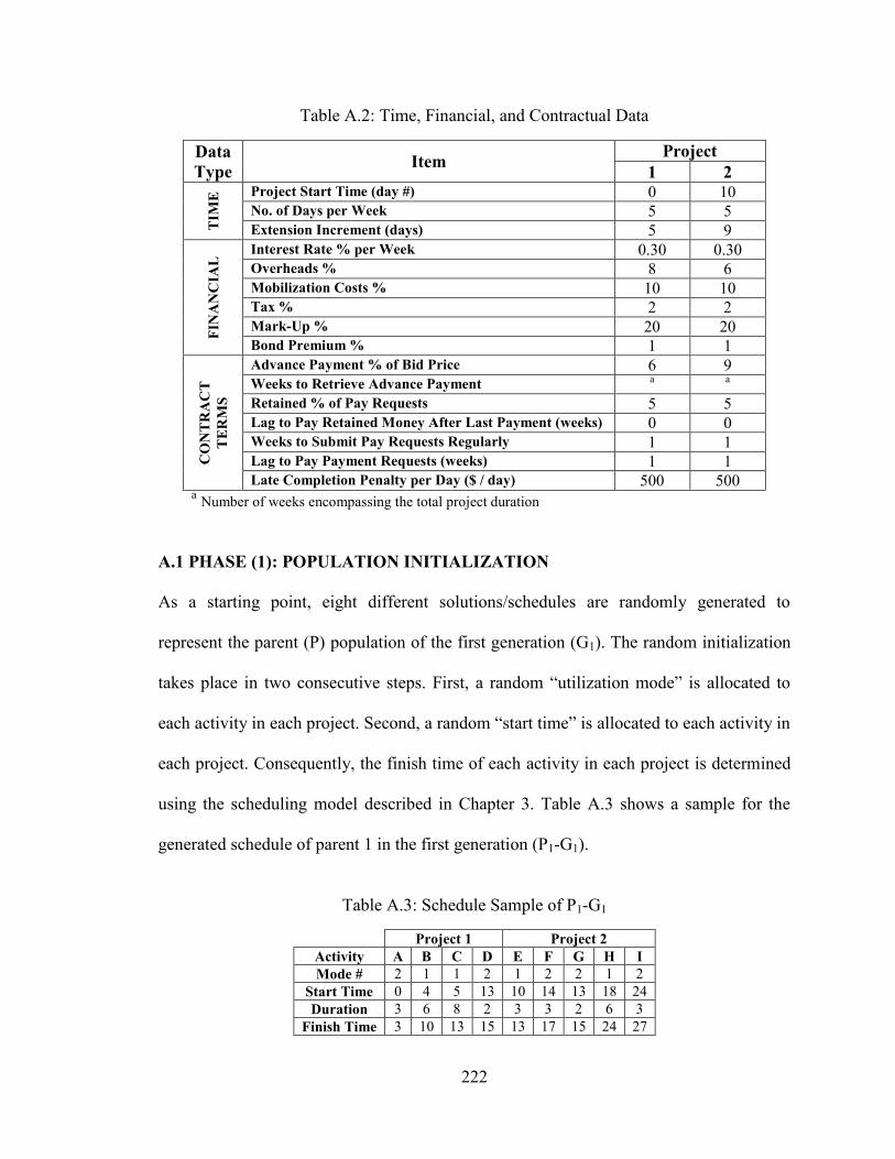
222
Table A.2: Time, Financial, and Contractual Data
Data
Type Item
Project
1 2
TIM
E Project Start Time (day #) 0 10
No. of Days per Week 5 5 Extension Increment (days) 5 9
FIN
AN
CIA
L Interest Rate % per Week 0.30 0.30
Overheads % 8 6 Mobilization Costs % 10 10 Tax % 2 2 Mark-Up % 20 20 Bond Premium % 1 1
CO
NT
RA
CT
TE
RM
S
Advance Payment % of Bid Price 6 9 Weeks to Retrieve Advance Payment a a
Retained % of Pay Requests 5 5 Lag to Pay Retained Money After Last Payment (weeks) 0 0 Weeks to Submit Pay Requests Regularly 1 1 Lag to Pay Payment Requests (weeks) 1 1 Late Completion Penalty per Day ($ / day) 500 500
a Number of weeks encompassing the total project duration
A.1 PHASE (1): POPULATION INITIALIZATION
As a starting point, eight different solutions/schedules are randomly generated to
represent the parent (P) population of the first generation (G1). The random initialization
takes place in two consecutive steps. First, a random “utilization mode” is allocated to
each activity in each project. Second, a random “start time” is allocated to each activity in
each project. Consequently, the finish time of each activity in each project is determined
using the scheduling model described in Chapter 3. Table A.3 shows a sample for the
generated schedule of parent 1 in the first generation (P1-G1).
Table A.3: Schedule Sample of P1-G1
Project 1 Project 2
Activity A B C D E F G H I
Mode # 2 1 1 2 1 2 2 1 2
Start Time 0 4 5 13 10 14 13 18 24
Duration 3 6 8 2 3 3 2 6 3
Finish Time 3 10 13 15 13 17 15 24 27

223
A.2 PHASE (2): FITNESS EVALUATION
After generating the initial parent population in phase 1, the optimization objectives are
to be determined. In other words, for each of the eight parent solutions generated, the FC,
RC, and PR are calculated using the cash flow model described earlier in Chapter 3.
Table A.4 shows the resulted objective values for each solution. It can be noticed that
solutions P6 and P8 are considered as “infeasible” solutions since their RC objective
values exceeded the set credit limit of $100,000.
Table A.4: Parent Population of First Generation (P-G1)
Solution OBJECTIVES
Feasibility FC RC PR
P1 682 96084 37848 Feasible
P2 728 93221 37904 Feasible
P3 678 75904 39115 Feasible
P4 659 71616 38382 Feasible
P5 785 84118 39479 Feasible
P6 681 101606 39379 Infeasible
P7 642 77767 38642 Feasible
P8 790 132100 37802 Infeasible
A.3 PHASE (3): GENERATION EVOLUTION
In this final phase, three types of population are to be generated as follows:
1. Child population of the first generation (Q-G1)
2. Combined population of the first generation (R-G1)
3. Parent population of the second generation (P-G2)
224
A.3.1 Child Population of the First Generation (Q-G1)
To generate the child population of the first generation, the following three steps are to be
applied:
Step 1: Non-Domination Rank Determination:
For each solution in the parent population of the first generation (P-G1), the non-
domination rank (irank) is to be determined. The ranking process takes place by comparing
the three objectives’ values (i.e. FC, RC, and PR) of each individual solution with those
of the other solutions. Consequently, the solutions are distributed to different “fronts” that
reflects their irank. When two solutions (X and Y) are compared at a time, two results are
expected. Either both solutions are non-dominated or one solution dominate the other. A
solution X dominates solution Y if:
1. Solution X is feasible and Solution Y is infeasible
2. Both solutions are infeasible and Solution X has a lower total constraint violation
than Solution Y.
3. Both solutions are feasible and Solution X dominates Solution Y. In other words,
Solution X have lower FC and RC values and higher PR value than those in
Solution Y.
Based on the above discussion, all of the eight solutions in P-G1 (see Table A.4) will be
considered in Front 1 as a starting point. After that, the comparison process will take
place as follows:

225
Front (1):
- P1 is compared with all the other solutions in front 1 as shown below:
Solutions Status Decision
P1 with P2 Non-dominated Keep both solutions in front 1
P1 with P3 P3 dominates P1 Keep P3 in front 1 and move P1 to front 2
- P2 is compared with all the other solutions left in front 1 as shown below:
Solutions Status Decision
P2 with P3 P3 dominates P2 Keep P3 in front 1 and move P2 to front 2
- P3 is compared with all the other solutions left in front 1 as shown below:
Solutions Status Decision
P3 with P4 Non-dominated Keep both solutions in front 1
P3 with P5 Non-dominated Keep both solutions in front 1
P3 with P6 P3 dominates P6 Keep P3 in front 1 and move P6 to front 2
P3 with P7 Non-dominated Keep both solutions in front 1
P3 with P8 P3 dominates P8 Keep P3 in front 1 and move P8 to front 2
- P4 is compared with all the other solutions left in front 1 as shown below:
Solutions Status Decision
P4 with P5 Non-dominated Keep both solutions in front 1
P4 with P7 Non-dominated Keep both solutions in front 1
- P5 is compared with all the other solutions left in front 1 as shown below:
Solutions Status Decision
P5 with P7 Non-dominated Keep both solutions in front 1
Thus, solutions P3, P4, P5, and P7 will remain in front 1.

226
Front (2):
- P1 is compared with all the other solutions in front 2 as shown below:
Solutions Status Decision
P1 with P2 Non-dominated Keep both solutions in front 2
P1 with P6 P1 dominates P6 Keep P1 in front 2 and move P6 to front 3
P1 with P8 P1 dominates P8 Keep P1 in front 2 and move P8 to front 3
Thus, solutions P1 and P2 will remain in front 2.
Front (3):
- P6 is compared with all the other solutions in front 3 as shown below:
Solutions Status Decision
P6 with P8 P6 dominates P8 Keep P6 in front 3 and move P8 to front 4
P6 dominated P8 since it has lower constraint violation. Thus, solution P6 will remain in
front 3 and P8 will be in front 4. Table A.5 summarizes the solutions distribution among
the different fronts.
Table A.5: Non-Domination Ranking of P-G1
Solution FRONT #
P3
Front 1 (irank = 1) P4
P5
P7
P1 Front 2 (irank = 2)
P2
P6 Front 3 (irank = 3)
P8 Front 4 (irank = 4)

227
Step 2: Crowding Distance Calculation:
The crowding distance (idistance) is calculated for fronts having more the one solution (i.e.
front 1 and 2) to determine the Euclidean distance between each individual in a front. The
calculation procedure is explained in details in Chapter 2. The boundary solutions
(solutions having the lowest or highest objective functions) in each front are assigned an
infinite distance value to keep diversity. Thus, solutions P4, P5, and P7 in front 1 and
solutions P1 and P2 in front 2 will have an infinite distance value. This leaves for us only
solution P3 in front 1 to calculate its crowding distance as follows:
- Sort the solutions in front 1 based on their objectives’ values from lowest to highest
as shown below:
Sorted
Solutions FC
Sorted
Solutions RC
Sorted
Solutions PR
P7 642 P4 71616 P4 38382
P4 659 P3 75904 P7 38642
P3 678 P7 77767 P3 39115
P5 785 P5 84118 P5 39479
- Calculate the crowding distance of P3 as shown below:
𝑖𝑑𝑖𝑠𝑡𝑎𝑛𝑐𝑒 (𝑃3) =(785 − 659)
(785 − 642)+
(77767 − 71616)
(84118 − 71616)+
(39479 − 38642)
(39479 − 38382)= 2.13
In real case analysis, when population size is large, it is uncommon to find most of the
solutions having infinite crowding distance.
Step 3: Tournament Selection, Crossover, and Mutation:
In order to generate the child population of the first generation, the parents should mate
first through crossover and/or mutation. However, the question that arises here is which

228
set of solutions in the parent population should be selected for the mating process. To
answer this question the following should be done:
- Since we have eight solutions, four mating rounds are to be established. Randomly
select any two solutions in the parent population twice for each round as shown
below:
Round # Sub-Round Solutions
1 1 P5 and P3
2 P1 and P8
2 1 P6 and P2
2 P5 and P7
3 1 P1 and P2
2 P3 and P4
4 1 P5 and P6
2 P7 and P8
- For each sub-round, select the winner solution according to the following:
Solution X wins Solution Y if irank(X) < irank(Y)
If both solutions have equal irank, then Solution X wins Solution Y if idistanceX >
idistanceY.
If both solutions have equal idistance, then randomly select anyone of them as a
winner.
As a result, the winner solutions from each sub-round is as shown below:
Round # Sub-Round Solutions Winner
1 1 P5 and P3 P5
2 P1 and P8 P1
2 1 P6 and P2 P2
2 P5 and P7 P7
3 1 P1 and P2 P2
2 P3 and P4 P4
4 1 P5 and P6 P5
2 P7 and P8 P7

229
Table A.6 summarizes the mating pool in which the crossover and/or mutation processes
will take place upon as discussed earlier in Chapter 4.
Table A.6: Mating Pool
Mating Pool # Solutions
1 P1 and P5
2 P2 and P7
3 P2 and P4
4 P5 and P7
Applying crossover and mutation processes on the above set of solutions will result in
generating eight new solutions that represent the child population of the first generation
(Q-G1). For each solution in Q-G1, the FC, RC, and PR objectives’ values are calculated
as explained before in step 2. Table A.7 shows the resulted objective values for each
solution.
Table A.7: Child Population of First Generation (Q-G1)
Solution OBJECTIVES
Feasibility FC RC PR
Q1 717 73334 38527 Feasible
Q2 731 90305 40693 Feasible
Q3 720 81240 38257 Feasible
Q4 657 87159 38280 Feasible
Q5 761 83864 38585 Feasible
Q6 619 84676 37707 Feasible
Q7 688 82264 40470 Feasible
Q8 704 77804 38744 Feasible
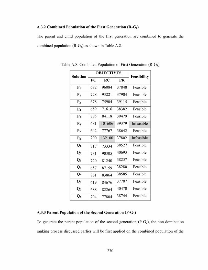
230
A.3.2 Combined Population of the First Generation (R-G1)
The parent and child population of the first generation are combined to generate the
combined population (R-G1) as shown in Table A.8.
Table A.8: Combined Population of First Generation (R-G1)
Solution OBJECTIVES
Feasibility FC RC PR
P1 682 96084 37848 Feasible
P2 728 93221 37904 Feasible
P3 678 75904 39115 Feasible
P4 659 71616 38382 Feasible
P5 785 84118 39479 Feasible
P6 681 101606 39379 Infeasible
P7 642 77767 38642 Feasible
P8 790 132100 37802 Infeasible
Q1 717 73334 38527 Feasible
Q2 731 90305 40693 Feasible
Q3 720 81240 38257 Feasible
Q4 657 87159 38280 Feasible
Q5 761 83864 38585 Feasible
Q6 619 84676 37707 Feasible
Q7 688 82264 40470 Feasible
Q8 704 77804 38744 Feasible
A.3.3 Parent Population of the Second Generation (P-G2)
To generate the parent population of the second generation (P-G2), the non-domination
ranking process discussed earlier will be first applied on the combined population of the

231
first generation (R-G1) shown in Table A.8. Table A.9 summarizes the solutions
distribution among the different fronts.
Table A.9: Non-Domination Ranking of R-G1
Solution FRONT #
P3
Front 1 (irank = 1)
P4
P7
Q1
Q2
Q6
Q7
P5
Front 2 (irank = 2) Q4
Q8
P1
Front 3 (irank = 3) Q3
Q5
P2 Front 4 (irank = 4)
P6 Front 5 (irank = 5)
P8 Front 6 (irank = 6)
The solutions of the parent population of the second generation will be selected from the
combined population giving the priority to those existing in front 1 then front 2 and so on
until the population size of eight is fulfilled. As shown in Table A.9, there are seven
solutions in front 1 which are to be taken for P-G2. Still, there will be one left solution to
be selected from front 2. The selection process will be according to the solution having
the highest crowding distance in front 2. Since the idistance for all the solutions in front 2 is
infinite, then one of them will be selected randomly to fulfill the eight required solutions
(assume solution P5). The same procedure is repeated according to the assigned number
of generations.
Top Related