


Languages
Pages
Legal


Chapter 16 -
MSNE 301 midterm #2 review October 2019
1
Chapter 6 - 2
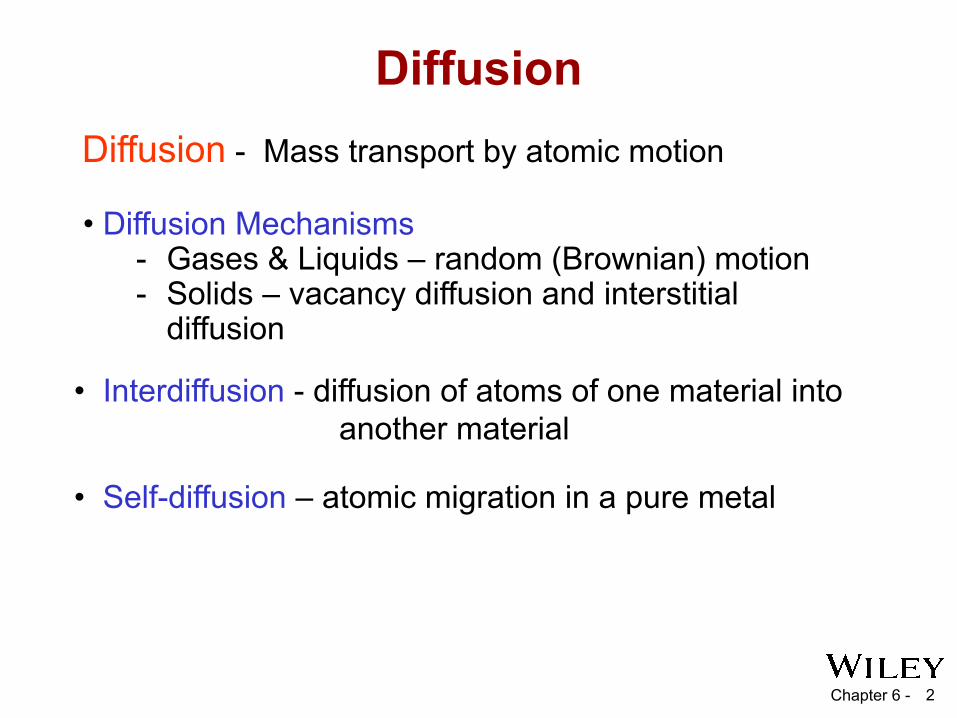
DiffusionDiffusion - Mass transport by atomic motion
• Interdiffusion - diffusion of atoms of one material into another material
• Self-diffusion – atomic migration in a pure metal
• Diffusion Mechanisms- Gases & Liquids – random (Brownian) motion- Solids – vacancy diffusion and interstitial
diffusion

Chapter 6 - 3
• Atoms tend to migrate from regions of high concentration to regions of low concentration.
Before diffusion
Figs. 6.1 & 6.2, Callister & Rethwisch 5e.
Diffusion
After diffusion
Concentration Profiles
Chapter 6 - 4
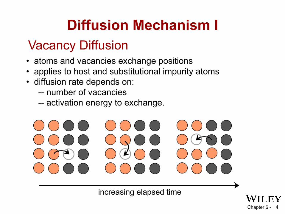
Diffusion Mechanism I
• atoms and vacancies exchange positions • applies to host and substitutional impurity atoms • diffusion rate depends on: -- number of vacancies -- activation energy to exchange.
increasing elapsed time
Vacancy Diffusion
Chapter 6 - 5
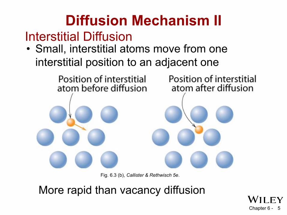
Diffusion Mechanism II
• Small, interstitial atoms move from one interstitial position to an adjacent one
More rapid than vacancy diffusionFig. 6.3 (b), Callister & Rethwisch 5e.
Interstitial Diffusion
Chapter 6 - 6
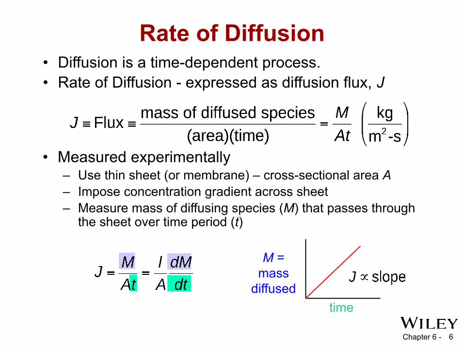
Rate of Diffusion• Diffusion is a time-dependent process.• Rate of Diffusion - expressed as diffusion flux, J
M =mass
diffusedtime
• Measured experimentally– Use thin sheet (or membrane) – cross-sectional area A– Impose concentration gradient across sheet– Measure mass of diffusing species (M) that passes through
the sheet over time period (t)
Chapter 6 - 7
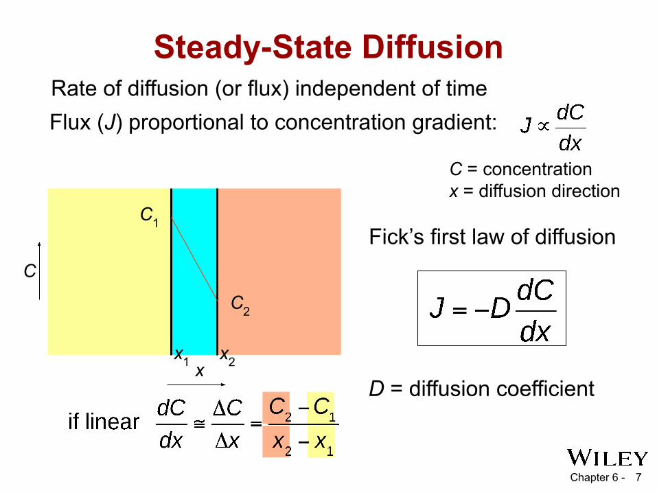
Steady-State Diffusion
Fick’s first law of diffusionC1
C2
x
C1
C2
x1 x2
D = diffusion coefficient
Rate of diffusion (or flux) independent of timeFlux (J) proportional to concentration gradient:
C = concentrationx = diffusion direction
C

Chapter 6 - 8
Influence of Temperature on Diffusion
• Diffusion coefficient increases with increasing T
D = Do exp − Qd
RT
= pre-exponential [m2/s]= diffusion coefficient [m2/s]
= activation energy [J/mol] = gas constant [8.314 J/mol-K]= absolute temperature [K]
DDo
Qd
RT

Chapter 6 - 9
transform data
D
Temp = T
ln D
1/T
Influence of Temperature on Diffusion (cont.)
take natural log of both sides
Chapter 6 - 10
Influence of Temperature on Diffusion (cont.)
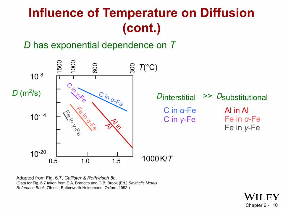
Adapted from Fig. 6.7, Callister & Rethwisch 5e. (Data for Fig. 6.7 taken from E.A. Brandes and G.B. Brook (Ed.) Smithells Metals Reference Book, 7th ed., Butterworth-Heinemann, Oxford, 1992.)
D has exponential dependence on T
Dinterstitial >> DsubstitutionalC in α-FeC in γ-Fe
Al in AlFe in α-FeFe in γ-Fe
1000 K/T
D (m2/s) C in α-Fe
C in γ-Fe
Al in
Al
Fe in α-Fe
Fe in γ-Fe
0.5 1.0 1.510-20
10-14
10-8T(°C)15
00
1000
600
300
Chapter 6 - 11
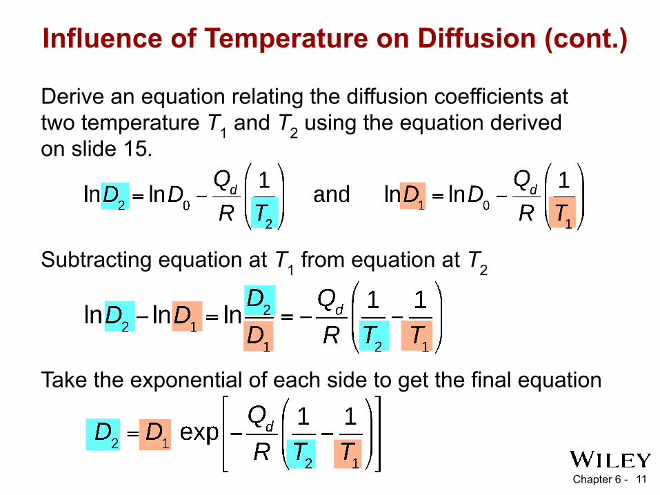
Influence of Temperature on Diffusion (cont.)
Subtracting equation at T1 from equation at T2
Derive an equation relating the diffusion coefficients at two temperature T1 and T2 using the equation derived on slide 15.
Take the exponential of each side to get the final equation
Chapter 6 - 12
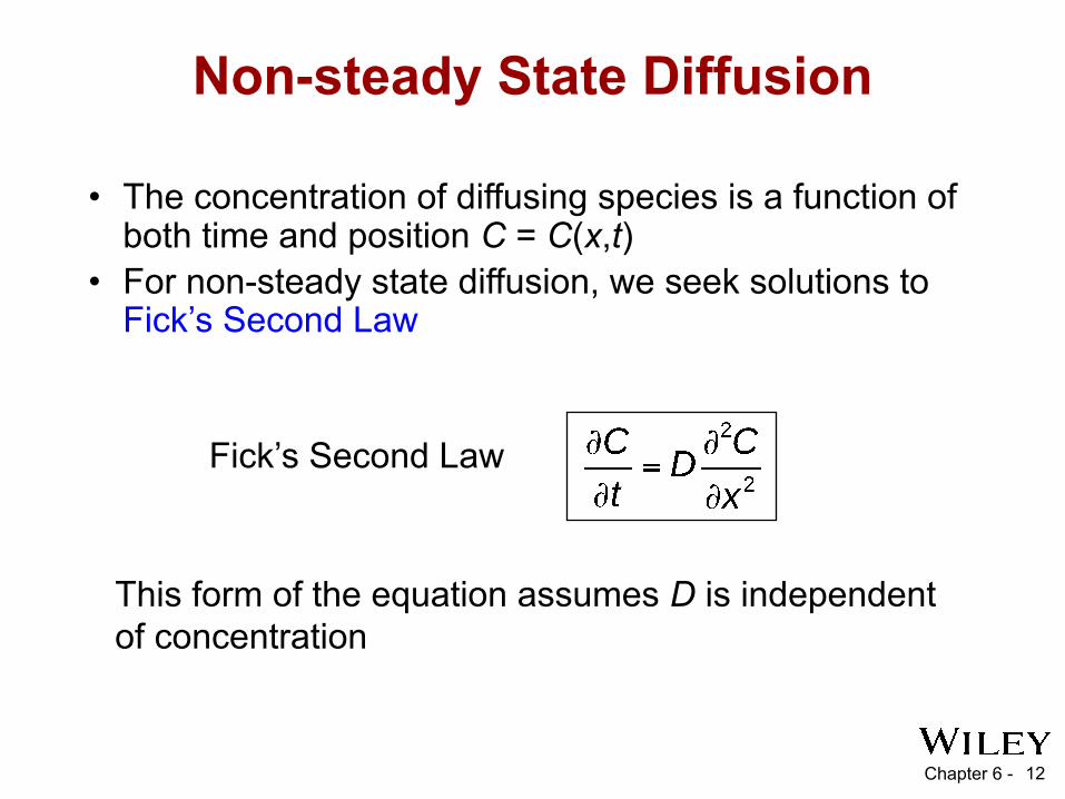
Non-steady State Diffusion
• The concentration of diffusing species is a function of both time and position C = C(x,t)
• For non-steady state diffusion, we seek solutions to Fick’s Second Law
Fick’s Second Law
This form of the equation assumes D is independent of concentration

Chapter 6 - 13
Non-steady State Diffusion
Fig. 6.5, Callister & Rethwisch 5e.
at t = 0, C = Co for 0 ≤ x ≤ ∞
at t > 0, C = CS for x = 0 (constant surface conc.)
C = Co for x = ∞
• Consider the diffusion of copper into a bar of aluminum
pre-existing conc., Co of copper atoms
Surface conc., C of Cu atoms bars
Cs
Boundary/Initial Conditions
Chapter 6 - 14
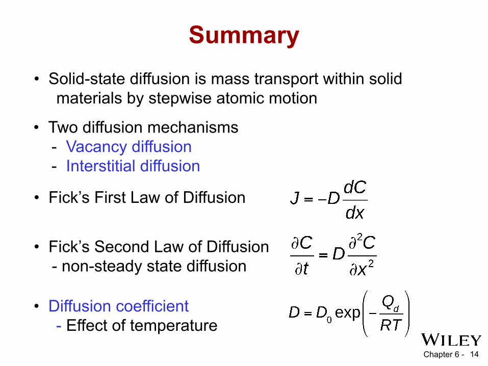
• Fick’s First Law of Diffusion
• Solid-state diffusion is mass transport within solid materials by stepwise atomic motion
Summary
• Two diffusion mechanisms - Vacancy diffusion - Interstitial diffusion
• Fick’s Second Law of Diffusion - non-steady state diffusion
• Diffusion coefficient - Effect of temperature

Chapter 6 - 15https://en.wikipedia.org/wiki/Dama
scus_steel

Chapter 7 - 16
ISSUES TO ADDRESS...• When a metal is exposed to mechanical forces, what parameters are used to express force magnitude and degree of deformation?• What is the distinction between elastic and plastic deformations? • How are the following mechanical characteristics of metals measured?
(a) Stiffness(b) Strength(c) Ductility(d) Hardness
• What parameters are used to quantify these properties?
Chapter 7: Mechanical Properties

Chapter 7 - 17
• Simple tension:
Δl = Fl oEAo
Δd = - ν FdoEAo
• Deflection is dependent on material, geometric, and loading parameters.• Materials with large elastic moduli deform less
Useful Linear Elastic Relationships
Ao
Adapted from Fig. 7.9, Callister & Rethwisch 5e.
Chapter 7 - 18
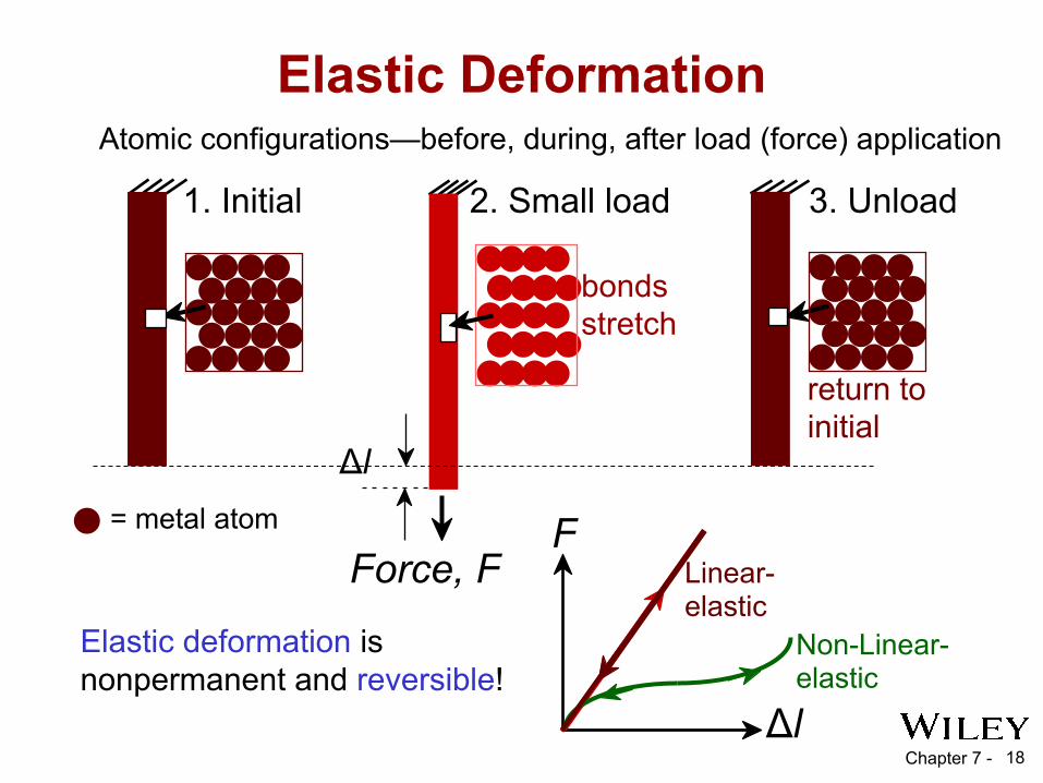
Elastic deformation is nonpermanent and reversible!
Elastic Deformation
2. Small load
Force, F
Δl
bonds stretch
1. Initial 3. Unload
return to initial
F
Δl
Linear- elastic
Non-Linear-elastic
Atomic configurations—before, during, after load (force) application
= metal atom

Chapter 7 - 19
Linear Elastic Properties
• Hooke's Law:σ = E ε
σ
Linear- elastic
• Modulus of Elasticity, E: (also known as Young's modulus)
E
ε
• Elastic deformation is nonpermanent and reversible! – generally valid at small deformations – linear stress strain curve
compression
tension
Units:E: [GPa] or [psi]1 GPa = 109 Pa

Chapter 7 - 20
Plastic Deformation
• Stress-strain plot for simple tension test:
stress, σ
strain, ε
Stressed into Plastic Region,Elastic + Plastic
εp
plastic strain
ElasticDeformation
Adapted from Fig. 7.10(a),Callister & Rethwisch 5e.
Stress Removed, Plastic Deformation Remains
• Plastic Deformation is permanent and nonrecoverable

Chapter 7 - 21
• Yield strength = stress at which noticeable plastic deformation has occurred
when εp = 0.002
Yield Strength
σy = yield strength
Note: for 5 cm sample
ε = 0.002 = Δz/z
Δz = 0.01 cm
Adapted from Fig. 6.10 (a),Callister & Rethwisch 9e.
σ (stress)
ε (strain)
σy
εp = 0.002
• Transition from elastic to plastic deformation is gradual
Chapter 7 - 22
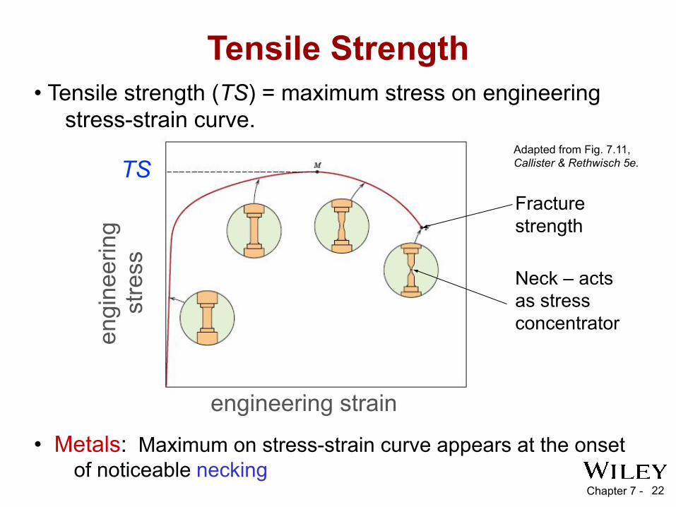
Tensile Strength
• Metals: Maximum on stress-strain curve appears at the onset of noticeable necking
Adapted from Fig. 7.11, Callister & Rethwisch 5e.
σy
strain
Typical response of a metal
Fracture strength
Neck – acts as stress concentrator
eng
inee
ring
TS s
tress
engineering strain
• Tensile strength (TS) = maximum stress on engineering stress-strain curve.

Chapter 7 - 23
• Ductility = amount of plastic deformation at failure:• Specification of ductility -- Percent elongation:
-- Percent reduction in area:
Ductility
lfAo Af
lo
Adapted from Fig. 7.13, Callister & Rethwisch 5e.
tensile strain, ε
tensile stress, σ
low ductility
high ductility
Chapter 7 - 24
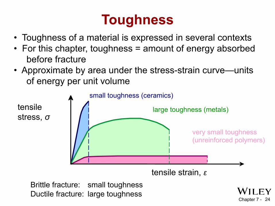
• Toughness of a material is expressed in several contexts • For this chapter, toughness = amount of energy absorbed before fracture • Approximate by area under the stress-strain curve—units of energy per unit volume
Toughness
Brittle fracture: small toughnessDuctile fracture: large toughness
very small toughness (unreinforced polymers)
tensile strain, ε
tensile stress, σ
small toughness (ceramics)
large toughness (metals)
Chapter 7 - 25
Mechanical PropertiesCeramic materials are more brittle than metals.
Why is this so?• Consider mechanism of deformation
– In crystalline, by dislocation motion– In highly ionic solids, dislocation motion is difficult
• few slip systems• resistance to motion of ions of like charge (e.g., anions) past
one another
Chapter 7 - 26
• Applied mechanical force—normalized to stress
• Elastic deformation:−−non-permanent; occurs at low levels of stress−−stress-strain behavior is linear
Summary
• Plastic deformation−−permanent; occurs at higher levels of stress−−stress-strain behavior is nonlinear
• Degree of deformation—normalized to strain
• Stiffness—a material's resistance to elastic deformation−−elastic (or Young's) modulus

Chapter 7 - 27
• Strength—a material's resistance to plastic deformation−−yield and tensile strengths
• Ductility—amount of plastic deformation at failure−−percents elongation, reduction in area
Summary (cont.)
• Hardness—resistance to localized surface deformation & compressive stresses
−−Rockwell, Brinell hardnesses
Chapter 8 - 28
ISSUES TO ADDRESS...• How are dislocations involved in the plastic deformation of materials?• Does the crystal structure of a material affect its mechanical characteristics? If so, how and why? • How are mechanical properties affected by dislocation mobilities?
Chapter 8: Deformation & Strengthening Mechanisms
• What techniques are used to increase the strength/hardness of metals/alloys?• How are mechanical characteristics of deformed metal specimens altered by heat treatments?
Chapter 8 - 29
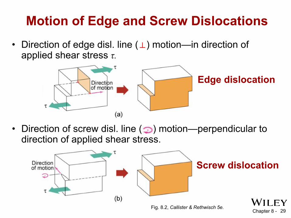
Motion of Edge and Screw Dislocations
• Direction of edge disl. line ( ) motion—in direction of applied shear stress τ.
Edge dislocation
Screw dislocation
Fig. 8.2, Callister & Rethwisch 5e.
• Direction of screw disl. line ( ) motion—perpendicular to direction of applied shear stress.
Chapter 8 - 30
Slip System—Combination of slip plane and slip direction – Slip Plane
• Crystallographic plane on which slip occurs most easily
• Plane with high planar density
– Slip Direction • Crystallographic direction along which slip occurs
most easily• Direction with high linear density
Slip Systems
Chapter 8 -
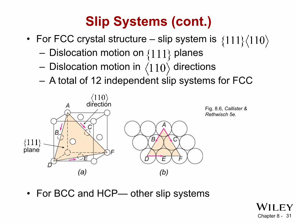
• For FCC crystal structure – slip system is– Dislocation motion on planes– Dislocation motion in directions– A total of 12 independent slip systems for FCC
31
Slip Systems (cont.)
Fig. 8.6, Callister & Rethwisch 5e.
direction
plane
• For BCC and HCP— other slip systems

Chapter 8 -
Slip in Single CrystalsResolved Shear Stress
• Applied tensile stress—shear stress component when slip plane oriented neither perpendicular nor parallel to stress direction
-- From figure, resolved shear stress, τR
32
ϕ
λ
• τR depends on orientation of normal to slip plane and slip direction with direction of tensile force F:
Fig. 8.7, Callister & Rethwisch 5e.
Chapter 8 - 33
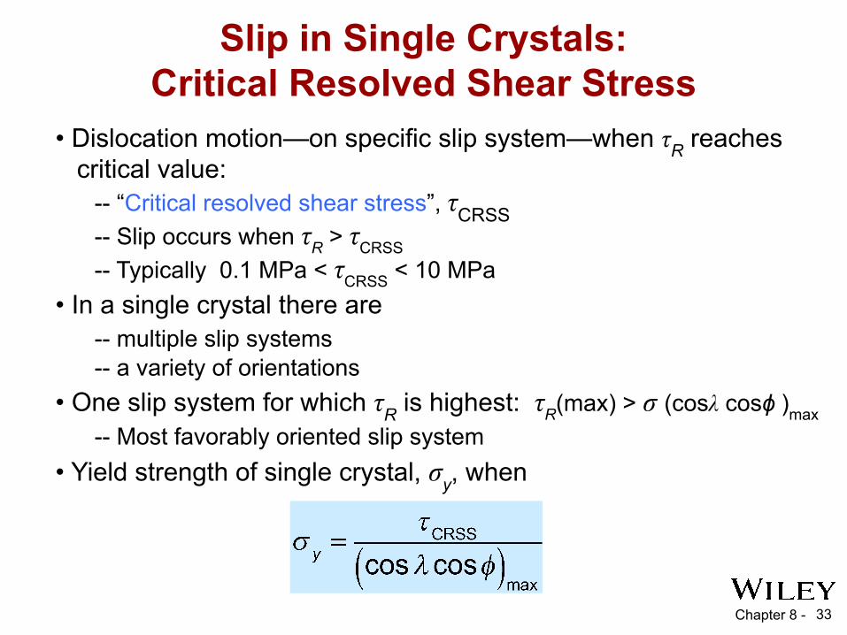
• Dislocation motion—on specific slip system—when τR reaches critical value: -- “Critical resolved shear stress”, τCRSS -- Slip occurs when τR > τCRSS -- Typically 0.1 MPa < τCRSS < 10 MPa
• One slip system for which τR is highest: τR(max) > σ (cosλ cosϕ )max -- Most favorably oriented slip system
Slip in Single Crystals:Critical Resolved Shear Stress
• In a single crystal there are -- multiple slip systems -- a variety of orientations
• Yield strength of single crystal, σy, when
Chapter 8 - 34
Strengthening Mechanisms for Metals • For a metal to plastically deform—dislocations must move
• Mechanisms for strengthening/hardening metals—decrease disl. mobility
• 3 mechanisms discussed -- Grain size reduction -- Solid solution strengthening -- Strain hardening (cold working)
• Strength and hardness—related to mobility of dislocations -- Reduce disl. mobility—metal strengthens/hardens -- Greater forces necessary to cause disl. motion -- Increase disl. mobility—metal becomes weaker/softer
Chapter 8 - 35
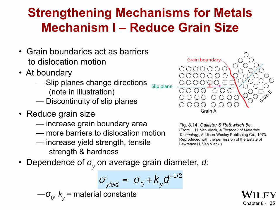
Strengthening Mechanisms for Metals Mechanism I – Reduce Grain Size
Fig. 8.14, Callister & Rethwisch 5e. (From L. H. Van Vlack, A Textbook of MaterialsTechnology, Addison-Wesley Publishing Co., 1973.Reproduced with the permission of the Estate ofLawrence H. Van Vlack.)
• Grain boundaries act as barriers to dislocation motion• At boundary — Slip planes change directions (note in illustration) — Discontinuity of slip planes• Reduce grain size — increase grain boundary area — more barriers to dislocation motion — increase yield strength, tensile strength & hardness• Dependence of σy on average grain diameter, d:
—σ0, ky = material constants

Chapter 8 - 36
Strengthening Mechanisms for MetalsMechanism II – Solid-Solution Strengthening
Fig. 8.4, Callister & Rethwisch 5e. (Adapted from W.G. Moffatt, G.W. Pearsall, and J. Wulff, The Structure and Properties of Materials, Vol. I, Structure, p. 140, John Wiley and Sons, New York, 1964.)
• Lattice strains around dislocations– Illustration notes locations of tensile, compressive
strains around an edge dislocation
Chapter 8 - 37
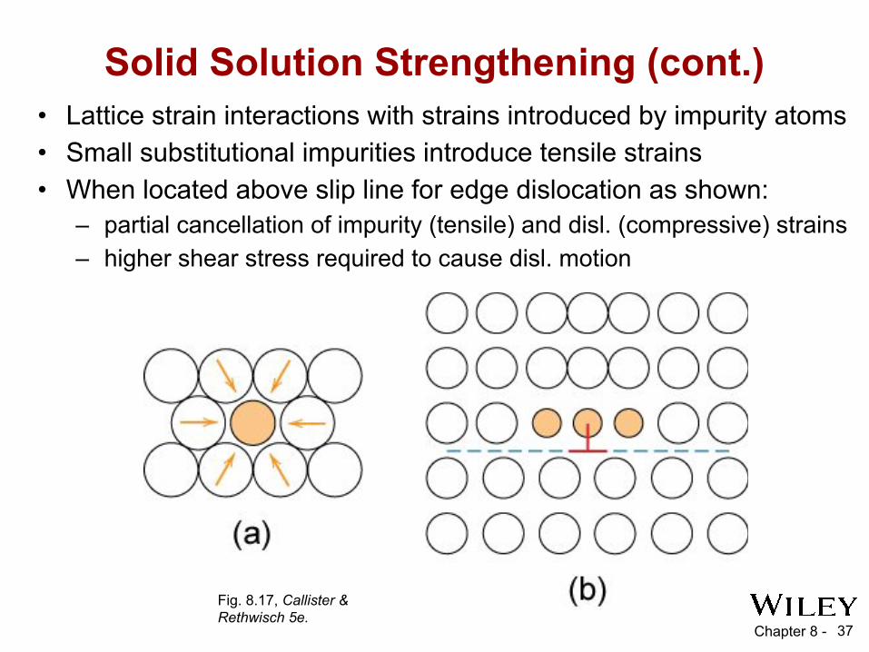
Solid Solution Strengthening (cont.)
Fig. 8.17, Callister & Rethwisch 5e.
• Lattice strain interactions with strains introduced by impurity atoms• Small substitutional impurities introduce tensile strains• When located above slip line for edge dislocation as shown:
– partial cancellation of impurity (tensile) and disl. (compressive) strains– higher shear stress required to cause disl. motion
Chapter 8 - 38
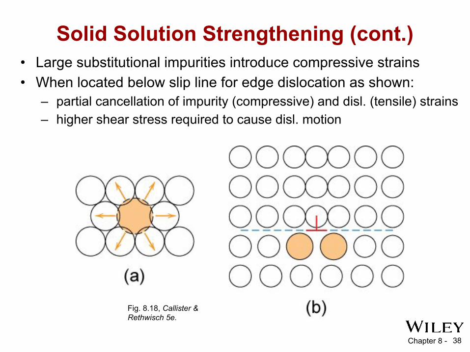
Solid Solution Strengthening (cont.)
Fig. 8.18, Callister & Rethwisch 5e.
• Large substitutional impurities introduce compressive strains• When located below slip line for edge dislocation as shown:
– partial cancellation of impurity (compressive) and disl. (tensile) strains– higher shear stress required to cause disl. motion
Chapter 8 - 39
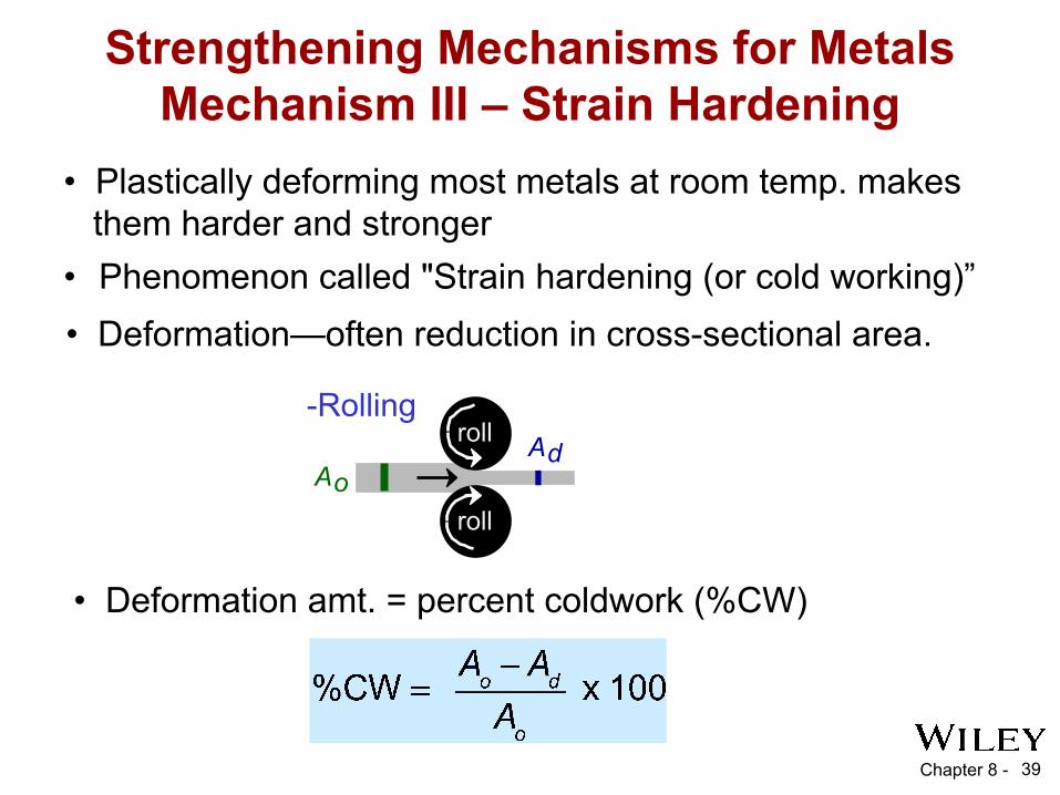
Strengthening Mechanisms for MetalsMechanism III – Strain Hardening
• Plastically deforming most metals at room temp. makes them harder and stronger • Phenomenon called "Strain hardening (or cold working)”
-Rolling
roll
AoAd
roll
• Deformation amt. = percent coldwork (%CW)
• Deformation—often reduction in cross-sectional area.
Chapter 8 - 40
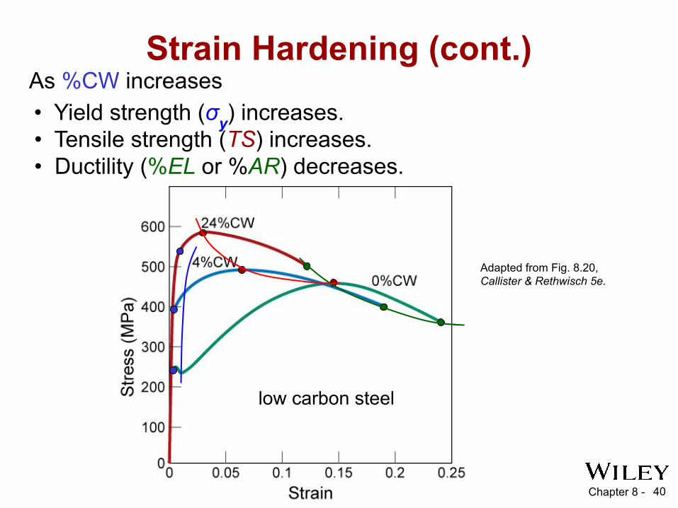
Strain Hardening (cont.)
Adapted from Fig. 8.20, Callister & Rethwisch 5e.
• Yield strength (σy) increases.• Tensile strength (TS) increases.• Ductility (%EL or %AR) decreases.
As %CW increases
low carbon steel
Chapter 8 - 41
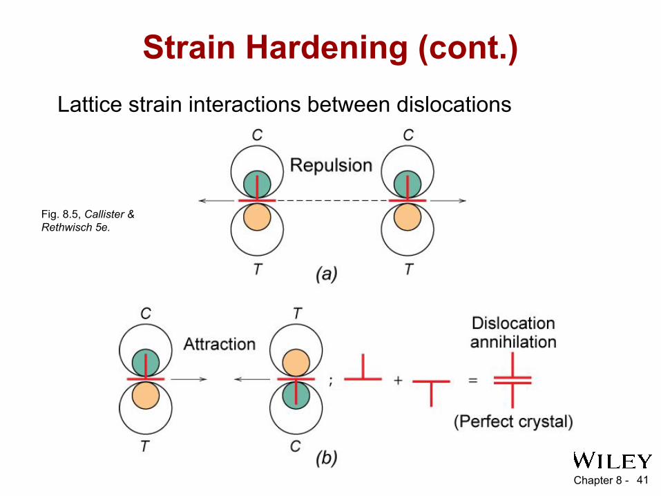
Strain Hardening (cont.)
Fig. 8.5, Callister & Rethwisch 5e.
Lattice strain interactions between dislocations

Chapter 8 - 42
Recovery
• Scenario 1
• Scenario 2
4. dislocations of oppositesign meet and annihilate
Dislocation annihilation- half-planescome together
extra half-plane of atoms
extra half-plane of atoms
atoms diffuse to regions of tension
2. grey atoms leave by vacancy diffusion allowing disl. to “climb”1. dislocation blocked; can’t move to the right
Obstacle dislocation
3. “Climbed” disl. can now move on new slip plane
During recovery – reduction in disl. density – annihilation of disl.
Chapter 8 - 43
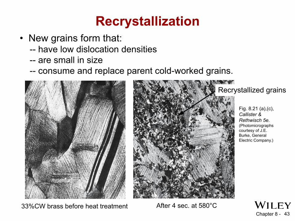
Fig. 8.21 (a),(c), Callister & Rethwisch 5e. (Photomicrographs courtesy of J.E. Burke, General Electric Company.)
33%CW brass before heat treatment
Recrystallized grains
Recrystallization• New grains form that: -- have low dislocation densities -- are small in size -- consume and replace parent cold-worked grains.
After 4 sec. at 580°C
Chapter 8 - 44
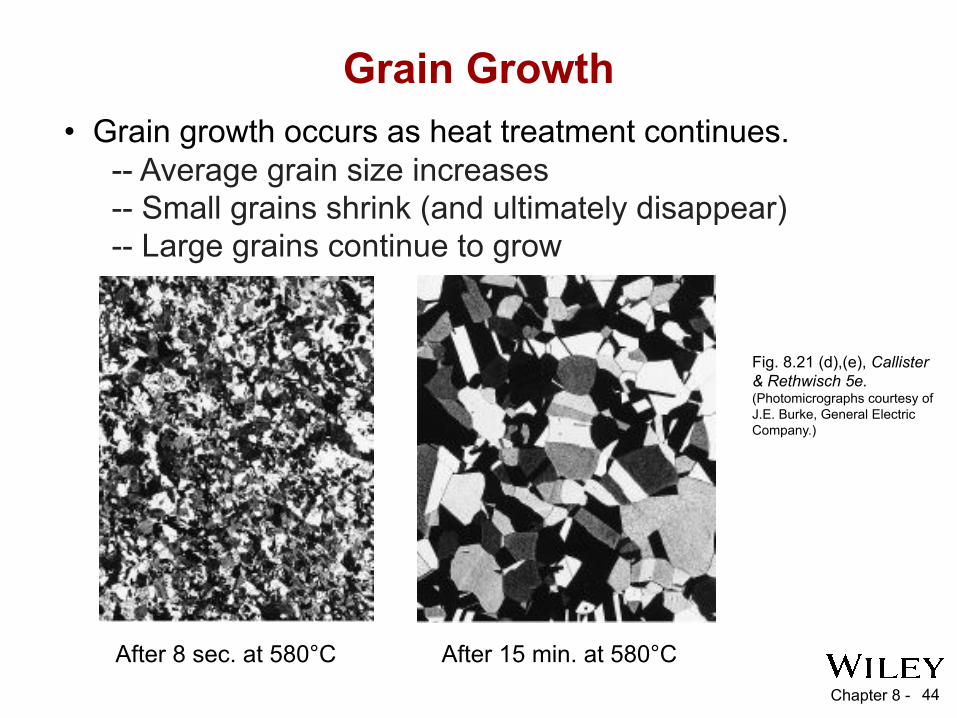
Fig. 8.21 (d),(e), Callister & Rethwisch 5e. (Photomicrographs courtesy of J.E. Burke, General Electric Company.)
Grain Growth• Grain growth occurs as heat treatment continues.
-- Average grain size increases-- Small grains shrink (and ultimately disappear)-- Large grains continue to grow
After 8 sec. at 580°C After 15 min. at 580°C
Chapter 8 - 45
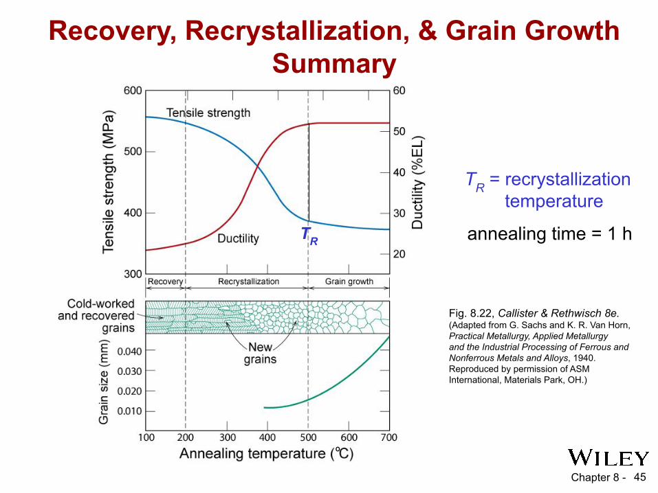
Fig. 8.22, Callister & Rethwisch 8e. (Adapted from G. Sachs and K. R. Van Horn,Practical Metallurgy, Applied Metallurgyand the Industrial Processing of Ferrous andNonferrous Metals and Alloys, 1940.Reproduced by permission of ASMInternational, Materials Park, OH.)
TR = recrystallization temperature
TR
º
Recovery, Recrystallization, & Grain GrowthSummary
annealing time = 1 h
Chapter 8 -
Grain Size Influences Properties
• Metals having small grains – relatively strong and tough at low temperatures
• Metals having large grains – good creep resistance at relatively high temperatures
46

Chapter 8 - 47
• Plastic deformation occurs by motion of dislocations
• Deformation of polycrystals—change of grain shapes
Summary
• Strengthening techniques for metals: -- grain size reduction -- solid solution strengthening -- strain hardening (cold working)
• Crystallographic considerations: -- Minimum atomic distortion from dislocation motion - in slip planes - along slip directions
• Strength is increased by decreasing dislocation mobility.
Chapter 8 - 48
Summary (cont.)
• Heat treatment of deformed metal specimens: -- Processes - Recovery - Recrystallization - Grain growth -- Consequences—property alterations - Softer and weaker - More ductile

Chapter 9 -
• Simple fracture – the separation of a body into two or more pieces in response to a static stress
• Propagation of cracks accompanies fracture
49
Fracture
• Two general types of fracture– Ductile
• Slow crack propagation• Accompanied by significant plastic deformation• Fails with warning
– Brittle• Rapid crack propagation• Little or no plastic deformation• Fails without warning
• Ductile fracture generally more desirable than brittle fracture
Chapter 9 -
• Fracture occurs as result of crack propagation • Measured fracture strengths of most materials
much lower than predicted by theory – microscopic flaws (cracks) always exist in materials– magnitude of applied tensile stress amplified at the
tips of these cracks
50
Principles of Fracture Mechanics
Chapter 9 - 51
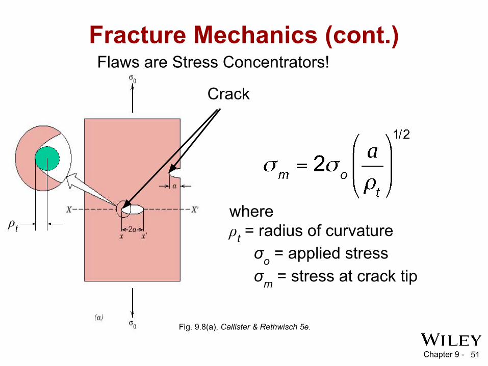
Fracture Mechanics (cont.)
where ρt = radius of curvature
σo = applied stressσm = stress at crack tip
ρt
Fig. 9.8(a), Callister & Rethwisch 5e.
Flaws are Stress Concentrators!
Crack
Chapter 9 - 52
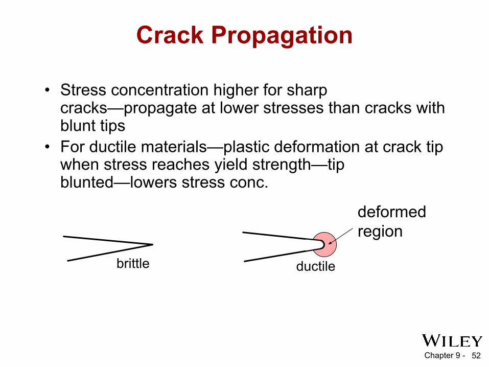
Crack Propagation
• Stress concentration higher for sharp cracks—propagate at lower stresses than cracks with blunt tips
• For ductile materials—plastic deformation at crack tip when stress reaches yield strength—tip blunted—lowers stress conc.
ductilebrittle
deformed region
Chapter 9 - 53
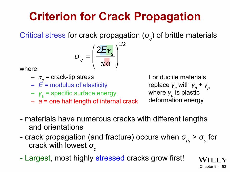
Criterion for Crack PropagationCritical stress for crack propagation (σc) of brittle materials
where– σc = crack-tip stress– E = modulus of elasticity– γs = specific surface energy– a = one half length of internal crack
For ductile materials replace γs with γs + γp where γp is plastic deformation energy
- materials have numerous cracks with different lengths and orientations
- crack propagation (and fracture) occurs when σm > σc for crack with lowest σc
- Largest, most highly stressed cracks grow first!

Chapter 9 -
Fracture Toughness• Measure of material’s resistance to brittle
fracture when a crack is present• Defined as
KC = YσC√π a
54
= dimensionless parameterY= critical stress for crack propagation [MPa] σc= crack length [m]a
= fracture toughness [MPa √m ]Kc
• For planar specimens with cracks much shorter than specimen width, Y ≈ 1
Chapter 9 - 55
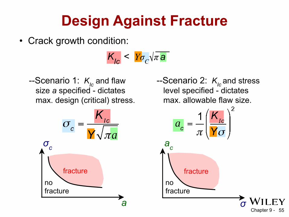
• Crack growth condition:
Design Against Fracture
--Scenario 1: KIc and flaw size a specified - dictates max. design (critical) stress.
σc
a
no fracture
fracture
--Scenario 2: KIc and stress level specified - dictates max. allowable flaw size.
ac
σ
no fracture
fracture
KIc < YσC√π a
Chapter 9 - 56
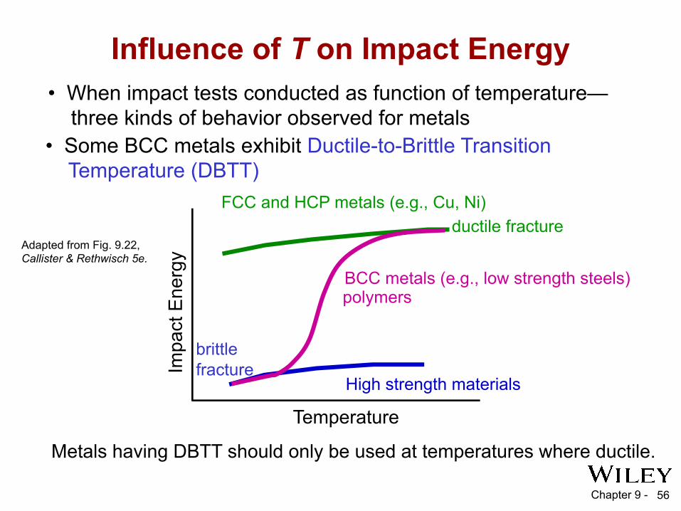
Influence of T on Impact Energy
Adapted from Fig. 9.22, Callister & Rethwisch 5e.
• Some BCC metals exhibit Ductile-to-Brittle Transition Temperature (DBTT)
• When impact tests conducted as function of temperature— three kinds of behavior observed for metals
BCC metals (e.g., low strength steels)
Impa
ct E
nerg
y
Temperature
High strength materials
polymers
FCC and HCP metals (e.g., Cu, Ni)ductile fracture
brittle fracture
Metals having DBTT should only be used at temperatures where ductile.

Chapter 9 - 57
Types of Fatigue Behavior
Adapted from Fig. 9.26(a), Callister & Rethwisch 5e.
- Fatigue limit, Sfat: no fatigue if S < Sfat
Sfat
case for steel (typ.)
N = Cycles to failure103 105 107 109
unsafe
safe
S =
stre
ss a
mpl
itude
- For some materials, there is no fatigue limit!
Adapted from Fig. 9.26(b), Callister & Rethwisch 5e.
case for Al (typ.)
N = Cycles to failure103 105 107 109
unsafe
safe
S =
stre
ss a
mpl
itude
• Fatigue data plotted as stress amplitude S vs. log of number N of cycles to failure.• Two types of fatigue behavior observed
• Fatigue Life Nf = total number of stress cycles to cause fatigue failure at specified stress amplitude
Chapter 9 - 58
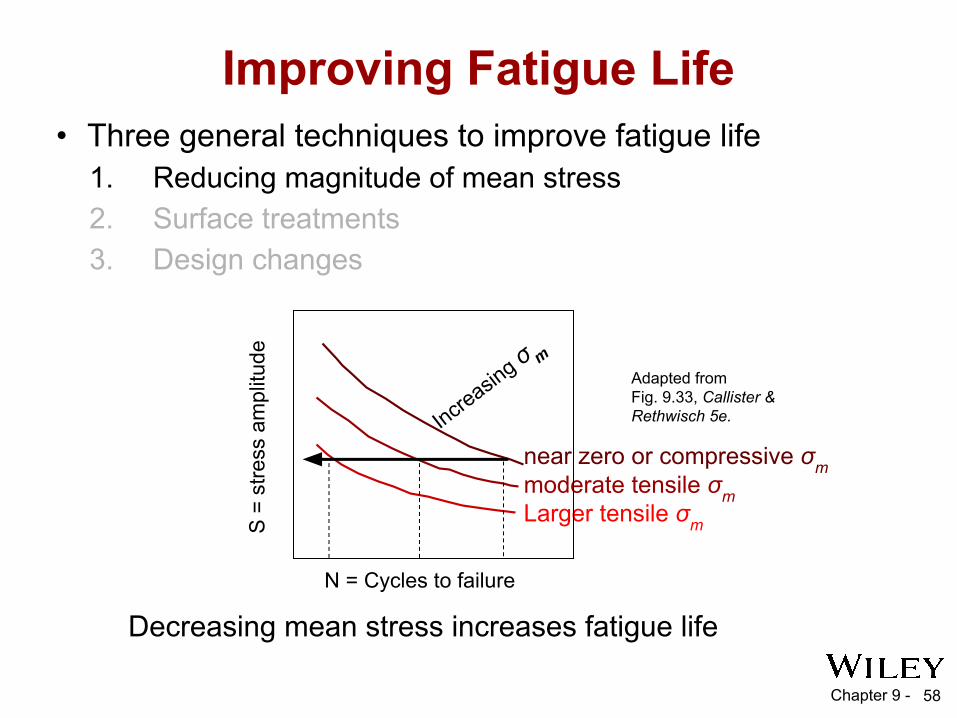
Improving Fatigue Life• Three general techniques to improve fatigue life
1. Reducing magnitude of mean stress2. Surface treatments3. Design changes
Adapted fromFig. 9.33, Callister & Rethwisch 5e.
N = Cycles to failure
moderate tensile σmLarger tensile σmS
= s
tress
am
plitu
de
near zero or compressive σm Incre
asing σ m
Decreasing mean stress increases fatigue life
Chapter 9 - 59
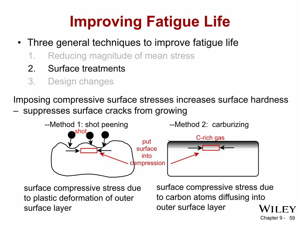
Improving Fatigue Life• Three general techniques to improve fatigue life
1. Reducing magnitude of mean stress2. Surface treatments3. Design changes
Imposing compressive surface stresses increases surface hardness – suppresses surface cracks from growing
--Method 1: shot peening
put surface
into compression
shot
surface compressive stress due to plastic deformation of outer surface layer
--Method 2: carburizing
C-rich gas
surface compressive stress due to carbon atoms diffusing into outer surface layer
Chapter 9 - 60
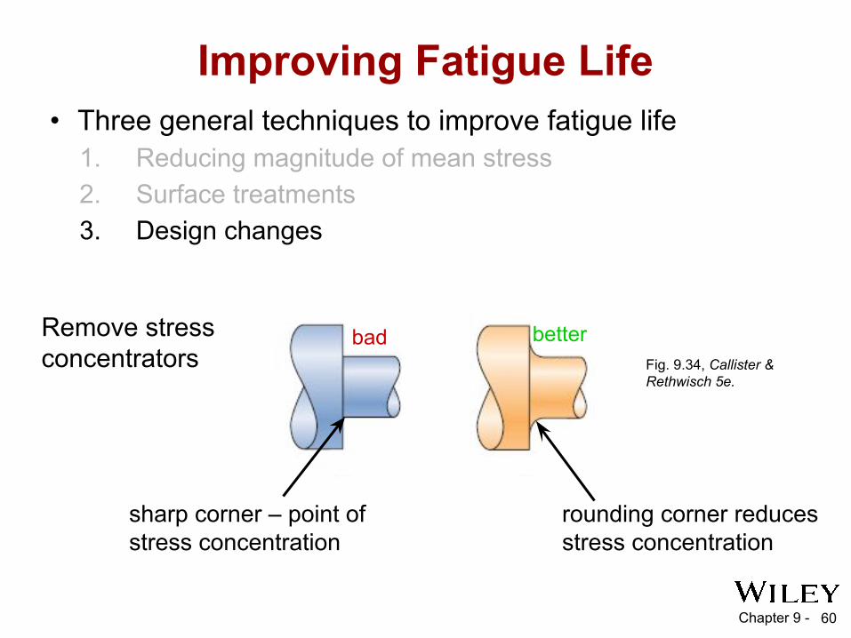
Improving Fatigue Life• Three general techniques to improve fatigue life
1. Reducing magnitude of mean stress2. Surface treatments3. Design changes
Remove stressconcentrators Fig. 9.34, Callister &
Rethwisch 5e.
bad better
sharp corner – point of stress concentration
rounding corner reduces stress concentration
Chapter 9 - 61
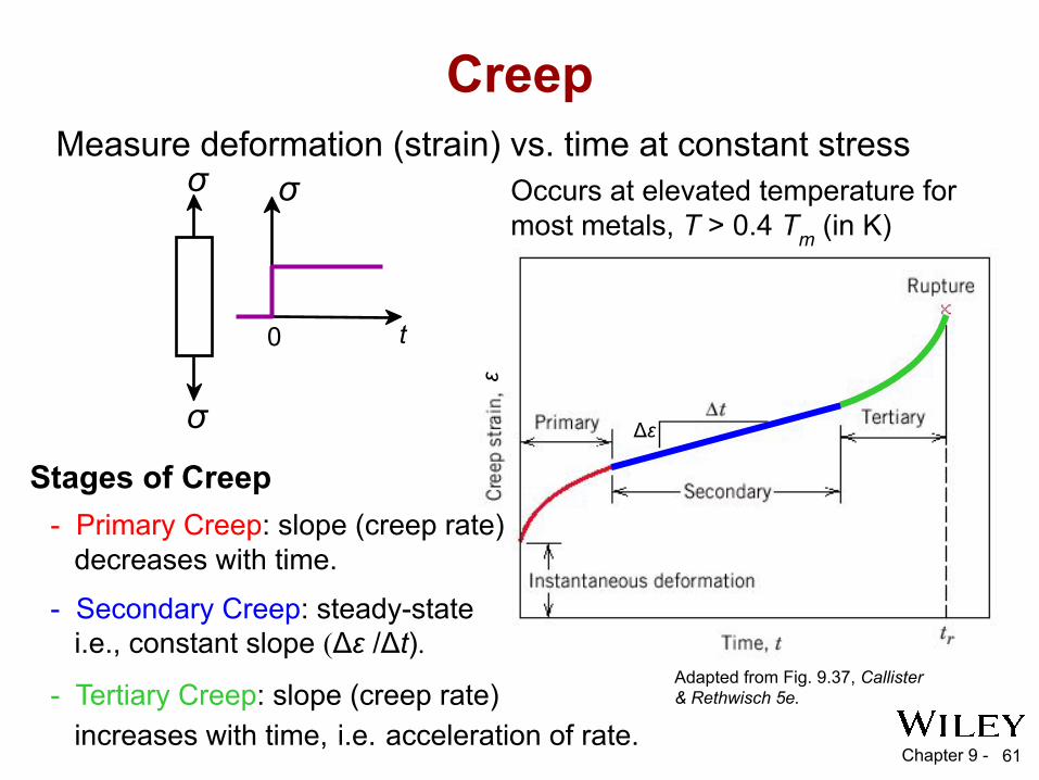
CreepMeasure deformation (strain) vs. time at constant stress
Adapted from Fig. 9.37, Callister & Rethwisch 5e.
σσ
0 t
σ
Occurs at elevated temperature for most metals, T > 0.4 Tm (in K)
Stages of Creep- Primary Creep: slope (creep rate) decreases with time.
- Secondary Creep: steady-state i.e., constant slope (Δε /Δt).
- Tertiary Creep: slope (creep rate) increases with time, i.e. acceleration of rate.
ε
Δε

Chapter 9 - 62
Steady-State Creep Rate• constant for constant T, σ -- strain hardening is balanced by recovery -- dependence of steady-state creep rate on T, σ
• Steady-state creep rate increases with increasing T, σ
102040
100200
10-2 10-1 1Steady state creep rate (%/1000hr)εs
Stre
ss (M
Pa) 427°C
538°C
649°C
Adapted fromFig. 9.40, Callister & Rethwisch 5e. [Reprinted with permission from Metals Handbook: Properties and Selection: Stainless Steels, Tool Materials, and Special Purpose Metals, Vol. 3, 9th ed., D. Benjamin (Senior Ed.), ASM International, 1980, p. 131.]
stress exponent (material parameter)
activation energy for creep(material parameter)
applied stressmaterial const.
Chapter 9 - 63
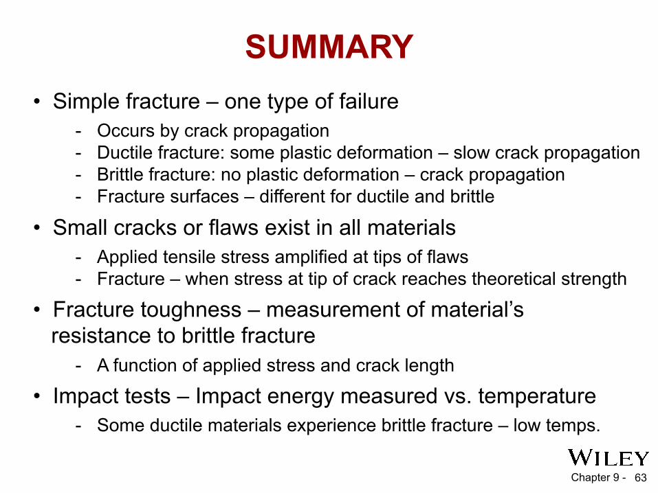
SUMMARY• Simple fracture – one type of failure
• Small cracks or flaws exist in all materials
• Fracture toughness – measurement of material’s resistance to brittle fracture
- Occurs by crack propagation- Ductile fracture: some plastic deformation – slow crack propagation- Brittle fracture: no plastic deformation – crack propagation- Fracture surfaces – different for ductile and brittle
- Applied tensile stress amplified at tips of flaws- Fracture – when stress at tip of crack reaches theoretical strength
- A function of applied stress and crack length
• Impact tests – Impact energy measured vs. temperature- Some ductile materials experience brittle fracture – low temps.

Chapter 9 - 64
SUMMARY (cont.)
• Fatigue failure – stress fluctuations with time
• Creep failure – at elevated temperatures and constant strain
- Occurs at applied stress < TS- Important parameters: fatigue limit, fatigue strength/lifetime
- Important parameters: steady-state creep rate, rupture lifetime- Data extrapolation – Larson-Miller parameter

Chapter 9 - 65
Phase Equilibria: Solubility Limit
Question: What is the solubility limit for sugar in water at 20°C?
Answer: 65 wt% sugar. At 20°C, if C < 65 wt% sugar: syrup At 20°C, if C > 65 wt% sugar:
syrup + sugar
65
• Solubility Limit: Maximum concentration for which only a single phase solution exists.
Sugar/Water Phase Diagram
Suga
r
Tem
pera
ture
(°C
)
0 20 40 60 80 100 C = Composition (wt% sugar)
L
(liquid solution i.e., syrup)
Solubility Limit L
(liquid) + S
(solid sugar)20
40
60
80
100
Wat
er
Adapted from Fig. 10.1, Callister & Rethwisch 5e.
• Solution – solid, liquid, or gas solutions, single phase• Mixture – more than one phase
Chapter 9 - 66
70 80 1006040200
Tem
pera
ture
(°C
)
C = Composition (wt% sugar)
L
(liquid solution i.e., syrup)
20
100
40
60
80
0
L (liquid)
+ S
(solid sugar)
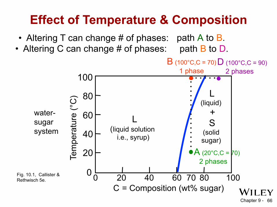
Effect of Temperature & Composition• Altering T can change # of phases: path A to B.
• Altering C can change # of phases: path B to D.
water-sugarsystem
Fig. 10.1, Callister & Rethwisch 5e.
D (100°C,C = 90)2 phases
B (100°C,C = 70)1 phase
A (20°C,C = 70)2 phases
Chapter 9 - 67
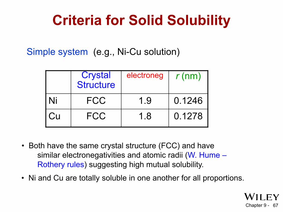
Criteria for Solid Solubility
CrystalStructure
electroneg r (nm)
Ni FCC 1.9 0.1246Cu FCC 1.8 0.1278
• Both have the same crystal structure (FCC) and have similar electronegativities and atomic radii (W. Hume – Rothery rules) suggesting high mutual solubility.
Simple system (e.g., Ni-Cu solution)
• Ni and Cu are totally soluble in one another for all proportions.
Chapter 9 -
wt% Ni20 40 60 80 10001000
1100
1200
1300
1400
1500
1600T(°C)
L (liquid)
α
(FCC solidsolution)
L + α
liquidus
solidusCu-Niphase
diagram
68
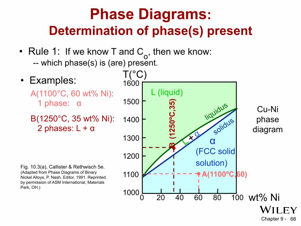
Phase Diagrams:Determination of phase(s) present
• Rule 1: If we know T and Co, then we know: -- which phase(s) is (are) present.
• Examples:A(1100°C, 60 wt% Ni): 1 phase: α
B(1250°C, 35 wt% Ni): 2 phases: L + α
B (1
250º
C,3
5) A(1100ºC,60)
Fig. 10.3(a), Callister & Rethwisch 5e. (Adapted from Phase Diagrams of BinaryNickel Alloys, P. Nash, Editor, 1991. Reprintedby permission of ASM International, MaterialsPark, OH.)

Chapter 9 - 69
• Rule 3: If we know T and C0, then can determine: -- the weight fraction of each phase.• Examples:
At TA: Only Liquid (L) present
WL = 1.00, Wα = 0
At TD:
Only Solid (α ) present
WL = 0, W
α = 1.00
Phase Diagrams:Determination of phase weight fractions
wt% Ni20
1200
1300
T(°C)
L (liquid)
α(solid)L + α
liquidus
solidus
30 40 50
L + α
Cu-Ni system
TAA
35C0
32CL
BTB
DTD
tie line
4Cα
3
R S
At TB:
Both α
and L present
= 0.27
WL= S
R +S
Wα= R
R +S
Consider C0 = 35 wt% Ni
Fig. 10.3(b), Callister & Rethwisch 5e. (Adapted from Phase Diagrams of BinaryNickel Alloys, P. Nash, Editor, 1991. Reprintedby permission of ASM International, MaterialsPark, OH.)
Chapter 9 - 70
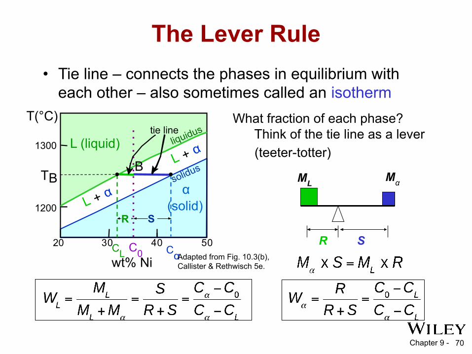
• Tie line – connects the phases in equilibrium with each other – also sometimes called an isotherm
The Lever Rule
What fraction of each phase? Think of the tie line as a lever (teeter-totter)
ML Mα
R S
wt% Ni20
1200
1300
T(°C)
L (liquid)
α(solid)L + α
liquidus
solidus
30 40 50
L + αB
TB
tie line
C0CL Cα
SR
Adapted from Fig. 10.3(b), Callister & Rethwisch 5e.
Chapter 9 - 71
wt% Ni20
1200
1300
30 40 50110 0
L (liquid)
α
(solid)
L + α
L + α
T(°C)
A
35C0
L: 35 wt%NiCu-Ni
system
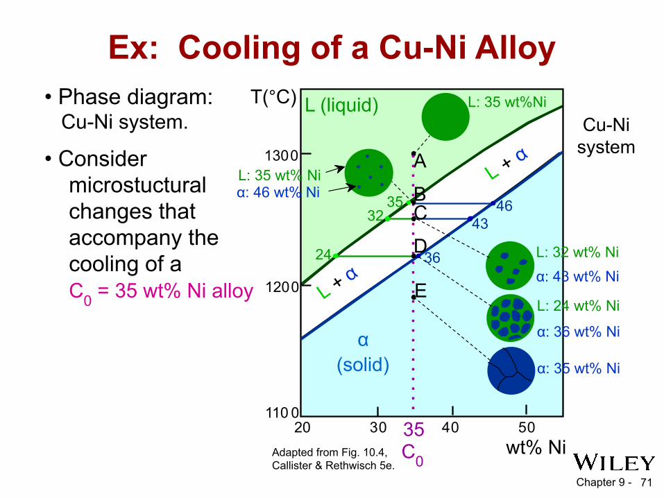
• Phase diagram: Cu-Ni system.
Adapted from Fig. 10.4, Callister & Rethwisch 5e.
• Consider microstuctural changes that accompany the cooling of a C0 = 35 wt% Ni alloy
Ex: Cooling of a Cu-Ni Alloy
46354332
α: 43 wt% Ni L: 32 wt% Ni
Bα: 46 wt% NiL: 35 wt% Ni
C
EL: 24 wt% Ni
α: 36 wt% Ni
24 36D
α: 35 wt% Ni

Chapter 9 - 72
L+αL+β
α + β
200
T(°C)
18.3
C, wt% Sn20 60 80 1000
300
100
L (liquid)
α 183°C
61.9 97.8β
• For a 40 wt% Sn-60 wt% Pb alloy at 150°C, determine: -- the phases present Pb-Sn
system
EX 1: Pb-Sn Eutectic System
Answer: α + β-- the phase compositions
-- the relative amount of each phase
150
40C0
11Cα
99Cβ
SR
Answer: Cα = 11 wt% SnCβ = 99 wt% Sn
Wα =Cβ - C0Cβ - Cα
= 99 - 4099 - 11 = 59
88 = 0.67
SR+S =
Wβ
=C0 - CαCβ - Cα
=RR+S
= 2988
= 0.33= 40 - 1199 - 11
Answer:
Fig. 10.8, Callister & Rethwisch 5e. [Adapted from Binary Alloy Phase Diagrams, 2nd edition, Vol. 3, T. B. Massalski (Editor-in-Chief), 1990. Reprinted by permission of ASM International, Materials Park, OH.]
Chapter 9 - 73
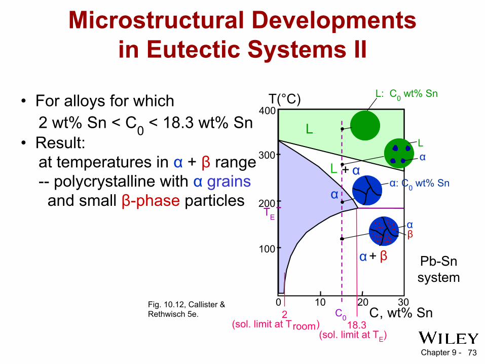
• For alloys for which 2 wt% Sn < C0 < 18.3 wt% Sn• Result: at temperatures in α + β range -- polycrystalline with α grains and small β-phase particles
Fig. 10.12, Callister & Rethwisch 5e.
Microstructural Developments in Eutectic Systems II
Pb-Snsystem
L + α
200
T(°C)
C, wt% Sn10
18.3
200C0
300
100
L
α
30
α + β
400
(sol. limit at TE)
TE
2(sol. limit at Troom)
Lα
L: C0 wt% Sn
αβ
α: C0 wt% Sn
Chapter 9 - 74
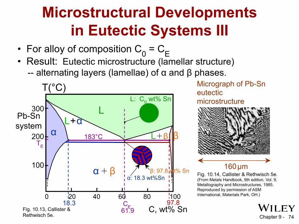
• For alloy of composition C0 = CE • Result: Eutectic microstructure (lamellar structure) -- alternating layers (lamellae) of α and β phases.
Fig. 10.13, Callister & Rethwisch 5e.
Microstructural Developments in Eutectic Systems III
Fig. 10.14, Callister & Rethwisch 5e. (From Metals Handbook, 9th edition, Vol. 9,Metallography and Microstructures, 1985.Reproduced by permission of ASM International, Materials Park, OH.)
160 μm
Micrograph of Pb-Sn eutectic microstructure
Pb-Snsystem
L + β
α + β
200
T(°C)
C, wt% Sn20 60 80 1000
300
100
L
α
βL+ α
183°C
40
TE
18.3
α: 18.3 wt%Sn
97.8
β: 97.8 wt% Sn
CE61.9
L: C0 wt% Sn

Chapter 9 - 75
L+αL+β
α + β
200
C, wt% Sn20 60 80 1000
300
100
L
α
βTE
40
(Pb-Sn System)
Hypoeutectic & Hypereutectic
Fig. 10.8, Callister & Rethwisch 5e. [Adapted from Binary Alloy Phase Diagrams, 2nd edition, Vol. 3, T. B. Massalski (Editor-in-Chief), 1990. Reprinted by permission of ASM International, Materials Park, OH.]
160 μmeutectic micro-constituent
Fig. 10.14, Callister & Rethwisch 5e.
hypereutectic: (illustration only)
β
βββ
β
β
Adapted from Fig. 10.17, Callister & Rethwisch 5e. (Illustration only)
(Figs. 9.14 and 9.17 from Metals Handbook, 9th ed., Vol. 9, Metallography and Microstructures, 1985.Reproduced by permission of ASM International,Materials Park, OH.)
175 μm
α
α
α
ααα
hypoeutectic: C0 = 50 wt% Sn
Fig. 10.17, Callister & Rethwisch 5e.
T(°C)
61.9eutectic
eutectic: C0 = 61.9 wt% Sn
Chapter 9 - 76
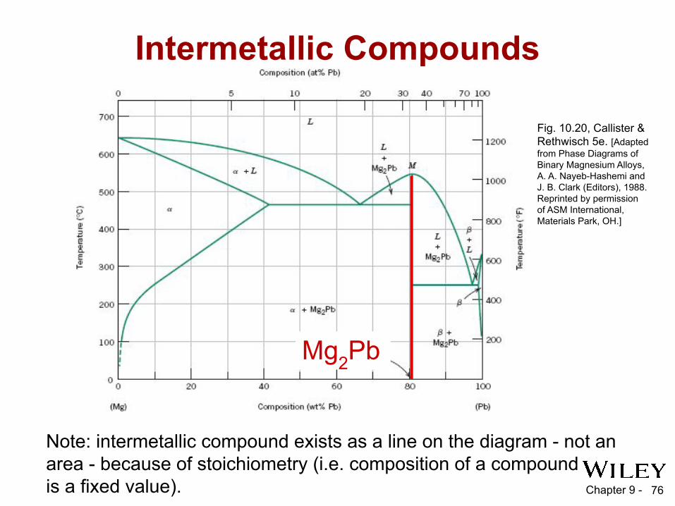
Intermetallic Compounds
Mg2Pb
Note: intermetallic compound exists as a line on the diagram - not an area - because of stoichiometry (i.e. composition of a compound is a fixed value).
Fig. 10.20, Callister & Rethwisch 5e. [Adapted from Phase Diagrams of Binary Magnesium Alloys, A. A. Nayeb-Hashemi and J. B. Clark (Editors), 1988. Reprinted by permission of ASM International, Materials Park, OH.]
Chapter 9 - 77
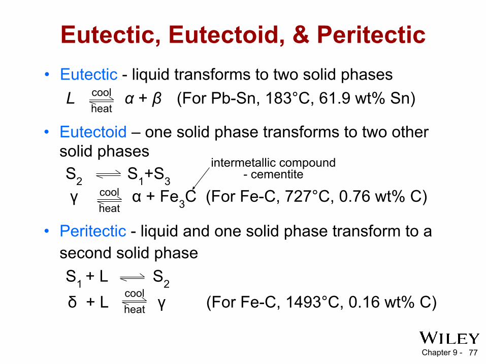
• Eutectoid – one solid phase transforms to two other solid phasesS2 S1+S3 γ α + Fe3C (For Fe-C, 727°C, 0.76 wt% C)
intermetallic compound - cementite
coolheat
Eutectic, Eutectoid, & Peritectic• Eutectic - liquid transforms to two solid phases
L α + β (For Pb-Sn, 183°C, 61.9 wt% Sn) coolheat
coolheat
• Peritectic - liquid and one solid phase transform to a second solid phase S1 + L S2
δ + L γ (For Fe-C, 1493°C, 0.16 wt% C)

Chapter 9 - 78
Eutectoid & PeritecticCu-Zn Phase diagram
Fig. 10.21, Callister & Rethwisch 5e. [Adapted from Binary Alloy Phase Diagrams, 2nd edition, Vol. 2, T. B. Massalski (Editor-in-Chief), 1990. Reprinted by permission of ASM International, Materials Park, OH.]
Eutectoid transformation δ γ + ε
Peritectic transformation γ + L δ
Chapter 9 - 79
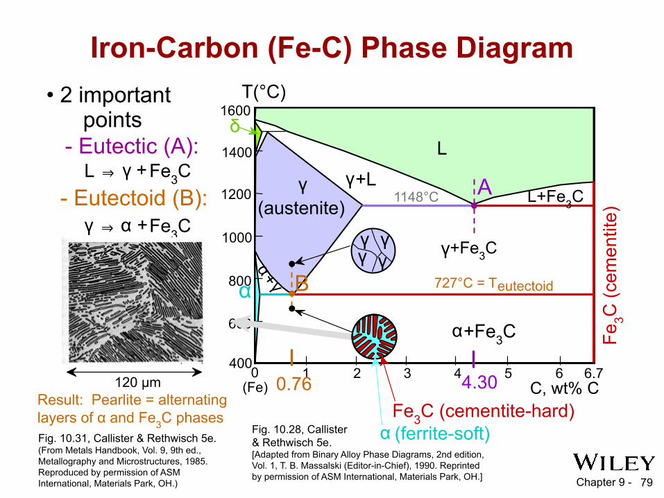
Iron-Carbon (Fe-C) Phase Diagram• 2 important points
- Eutectoid (B):
γ ⇒ α +Fe3C
- Eutectic (A):
L ⇒ γ +Fe3C
Fig. 10.28, Callister & Rethwisch 5e. [Adapted from Binary Alloy Phase Diagrams, 2nd edition, Vol. 1, T. B. Massalski (Editor-in-Chief), 1990. Reprinted by permission of ASM International, Materials Park, OH.]
Fe3C
(cem
entit
e)
1600
1400
1200
1000
800
600
4000 1 2 3 4 5 6 6.7
L
γ (austenite)
γ+L
γ+Fe3C
α+Fe3C
α+ γ
δ
(Fe) C, wt% C
1148°C
T(°C)
α 727°C = Teutectoid
4.30Result: Pearlite = alternatinglayers of α and Fe3C phases
120 μm
Fig. 10.31, Callister & Rethwisch 5e. (From Metals Handbook, Vol. 9, 9th ed.,Metallography and Microstructures, 1985.Reproduced by permission of ASM International, Materials Park, OH.)
0.76
Bγ γ
γγ
A L+Fe3C
Fe3C (cementite-hard)α (ferrite-soft)
Chapter 9 - 80Fe
3C (c
emen
tite)
1600
1400
1200
1000
800
600
4000 1 2 3 4 5 6 6.7
L
γ (austenite)
γ+L
γ + Fe3C
α + Fe3C
L+Fe3C
δ
(Fe) C, wt% C
1148°C
T(°C)
α727°C
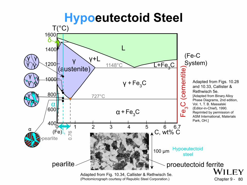
(Fe-C System)
C0
0.76
Hypoeutectoid Steel
Adapted from Figs. 10.28 and 10.33, Callister & Rethwisch 5e. [Adapted from Binary Alloy Phase Diagrams, 2nd edition, Vol. 1, T. B. Massalski (Editor-in-Chief), 1990. Reprinted by permission of ASM International, Materials Park, OH.]
Adapted from Fig. 10.34, Callister & Rethwisch 5e. (Photomicrograph courtesy of Republic Steel Corporation.)
proeutectoid ferritepearlite
100 μm Hypoeutectoidsteel
α
pearlite
γγ γ
γααα
γγγ γ
γ γγγ
Chapter 9 -Fe
3C (c
emen
tite)
1600
1400
1200
1000
800
600
4000 1 2 3 4 5 6 6.7
L
γ (austenite)
γ+L
γ + Fe3C
α + Fe3C
L+Fe3C
δ
(Fe) C, wt% C
1148°C
T(°C)
α727°C
(Fe-C System)
C0
81
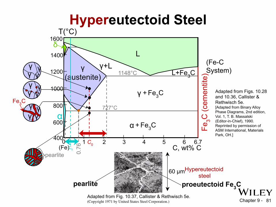
Hypereutectoid Steel
0.76
C0
Fe3C
γγγ γ
γγγ γ
γγγ γ
Adapted from Fig. 10.37, Callister & Rethwisch 5e. (Copyright 1971 by United States Steel Corporation.)
proeutectoid Fe3C
60 μmHypereutectoid steel
pearlite
pearlite
Adapted from Figs. 10.28 and 10.36, Callister & Rethwisch 5e. [Adapted from Binary Alloy Phase Diagrams, 2nd edition, Vol. 1, T. B. Massalski (Editor-in-Chief), 1990. Reprinted by permission of ASM International, Materials Park, OH.]
Chapter 9 - 82
Chapter 9 - 83
• Heat treatments of Fe-C alloys produce microstructures including: -- pearlite, bainite, spheroidite, martensite, tempered martensite• Precipitation hardening --hardening, strengthening due to formation of precipitate particles. --Al, Mg alloys precipitation hardenable.• Polymer melting and glass transition temperatures
Summary

Chapter 9 - 84
• Phase diagrams are useful tools to determine:-- the number and types of phases present,-- the composition of each phase,-- and the weight fraction of each phase given the temperature and composition of the system.
• The microstructure of an alloy depends on -- its composition, and -- whether or not cooling rate allows for maintenance of equilibrium.
• Important phase diagram phase transformations include eutectic, eutectoid, and peritectic.
Summary
Top Related