


Languages
Pages
Legal


Model reduction of large-scale systemsLecture I: Overview
Thanos Antoulas
Rice University and Jacobs University
email: [email protected]: www.ece.rice.edu/ aca
International School, Monopoli, 7-12 September 2008
Thanos Antoulas (Rice U. & Jacobs U.) Model reduction of large-scale systems 1 / 36
Outline
1 Introduction and model reduction problemThe big pictureProblem formulationProjections
2 Motivating examples
3 Overview of approximation methodsSVDPODBalanced truncationKrylov methodsMoment matching
4 Summary – Challenges – References
Thanos Antoulas (Rice U. & Jacobs U.) Model reduction of large-scale systems 2 / 36

Introduction and model reduction problem
Outline
1 Introduction and model reduction problemThe big pictureProblem formulationProjections
2 Motivating examples
3 Overview of approximation methodsSVDPODBalanced truncationKrylov methodsMoment matching
4 Summary – Challenges – References
Thanos Antoulas (Rice U. & Jacobs U.) Model reduction of large-scale systems 3 / 36

Introduction and model reduction problem The big picture
The big picture
@@
@@
@@R
��
��
��
@@
@@
@@R
� discretization
Modeling
Model reduction
���*
HHHj
Simulation
Controlreduced # of ODEs
ODEs PDEs
��
��
��
��
��
��
��
��
��
��
��
��
��
��
Physical System and/or Data
Thanos Antoulas (Rice U. & Jacobs U.) Model reduction of large-scale systems 4 / 36

Introduction and model reduction problem Problem formulation
Dynamical systems
x1(·)x2(·)
...xn(·)
u1(·) −→u2(·) −→
...um(·) −→
−→ y1(·)−→ y2(·)
...−→ yp(·)
We consider explicit state equations
Σ : x(t) = f(x(t), u(t)), y(t) = h(x(t), u(t))
with state x(·) of dimension n � m, p.
Thanos Antoulas (Rice U. & Jacobs U.) Model reduction of large-scale systems 5 / 36

Introduction and model reduction problem Problem formulation
Problem statement
Given: dynamical system
Σ = (f, h) with: u(t) ∈ Rm, x(t) ∈ Rn, y(t) ∈ Rp.
Problem: Approximate Σ with:
Σ = (f, h) with : u(t) ∈ Rm, x(t) ∈ Rk , y(t) ∈ Rp, k � n :
(1) Approximation error small - global error bound
(2) Preservation of stability/passivity
(3) Procedure must be computationally efficient
Thanos Antoulas (Rice U. & Jacobs U.) Model reduction of large-scale systems 6 / 36

Introduction and model reduction problem Projections
Approximation by projection
Unifying feature of approximation methods: projections.
Let V, W ∈ Rn×k , such that W∗V = Ik ⇒ Π = VW∗ is a projection.Define x = W∗x. Then
Σ :
{ddt x(t) = W∗f(Vx(t), u(t))
y(t) = h(Vx(t), u(t))
Thus Σ is ”good” approximation of Σ, if x− Πx is ”small”.
Thanos Antoulas (Rice U. & Jacobs U.) Model reduction of large-scale systems 7 / 36

Introduction and model reduction problem Projections
Special case: linear dynamical systems
Σ: Ex(t) = Ax(t) + Bu(t), y(t) = Cx(t) + Du(t)
Σ =
(E, A BC D
)Problem: Approximate Σ by projection: Π = VW∗
Σ =
(E, A BC D
)=
(W∗EV, W∗AV W∗B
CV D
), k � n
Norms:• H∞-norm:worst output error‖y(t)− y(t)‖ for ‖u(t)‖ = 1.
• H2-norm: ‖h(t)− h(t)‖
E, An
n
C
B
D
⇒ E, Ak
k
C
B
D
Σ: : Σ
= Vn
k
W∗
Thanos Antoulas (Rice U. & Jacobs U.) Model reduction of large-scale systems 8 / 36

Motivating examples
Outline
1 Introduction and model reduction problemThe big pictureProblem formulationProjections
2 Motivating examples
3 Overview of approximation methodsSVDPODBalanced truncationKrylov methodsMoment matching
4 Summary – Challenges – References
Thanos Antoulas (Rice U. & Jacobs U.) Model reduction of large-scale systems 9 / 36

Motivating examples
Motivating Examples: Simulation/Control
1. Passive devices • VLSI circuits• Thermal issues• Power delivery networks
2. Data assimilation • North sea forecast• Air quality forecast
3. Molecular systems • MD simulations• Heat capacity
4. CVD reactor • Bifurcations5. Mechanical systems: •Windscreen vibrations
• Buildings6. Optimal cooling • Steel profile7. MEMS: Micro Electro-
-Mechanical Systems • Elf sensor8. Nano-Electronics • Plasmonics
Thanos Antoulas (Rice U. & Jacobs U.) Model reduction of large-scale systems 10 / 36
Motivating examples
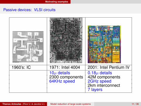
Passive devices: VLSI circuits
1960’s: IC 1971: Intel 4004 2001: Intel Pentium IV10µ details 0.18µ details2300 components 42M components64KHz speed 2GHz speed
2km interconnect7 layers
Thanos Antoulas (Rice U. & Jacobs U.) Model reduction of large-scale systems 11 / 36

Motivating examples
Passive devices: VLSI circuits
Typical GateDelay
0.1
1.0D
elay
(ns)
1.01.3 0.8 0.30.5Technology (μm)
0.1 0.08
Average WiringDelay
≈ 0.25 μm
Today’s Technology: 65 nm
65nm technology: gate delay < interconnect delay!
Conclusion: Simulations are required to verify that internal electromagneticfields do not significantly delay or distort circuit signals. Thereforeinterconnections must be modeled.
⇒ Electromagnetic modeling of packages and interconnects ⇒ resultingmodels very complex: using PEEC methods (discretization of Maxwell’sequations): n ≈ 105 · · · 106 ⇒ SPICE: inadequate
• Source: van der Meijs (Delft)Thanos Antoulas (Rice U. & Jacobs U.) Model reduction of large-scale systems 12 / 36

Motivating examples
Power delivery network for VLSI chips
VDD
r r r rr r r r
r r r rr r r r�
��
��
��
���
��
��
��
��
��
��
��
��
��
��
��
��
��
��
��
AA AA AA AA
AA AA AA AA
AA AA AA AA
AA AA AA AA
n? n?
r r'
&
$
%
'&
$%
?
R L
C C
#states ≈ 8 · 106
#inputs/outputs ≈ 1 · 106
1
Thanos Antoulas (Rice U. & Jacobs U.) Model reduction of large-scale systems 13 / 36

Motivating examples
Mechanical systems: carsCar windscreen simulation subject to acceleration load.
Problem: compute noise at points away from the window.PDE: describes deformation of a structure of a specific material; FEdiscretization: 7564 nodes (3 layers of 60 by 30 elements). Material:glass with Young modulus 7·1010 N/m2; density 2490 kg/m3; Poissonratio 0.23 ⇒ coefficients of FE model determined experimentally.The discretized problem has dimension: 22,692.
Notice: this problem yields 2nd order equations:
Mx(t) + Cx(t) + Kx(t) = f(t).
• Source: Meerbergen (Free Field Technologies)
Thanos Antoulas (Rice U. & Jacobs U.) Model reduction of large-scale systems 14 / 36

Motivating examples
Mechanical Systems: BuildingsEarthquake prevention
Taipei 101: 508m Damper between 87-91 floors 730 ton damper
Building Height Control mechanism Damping frequencyDamping mass
CN Tower, Toronto 533 m Passive tuned mass damperHancock building, Boston 244 m Two passive tuned dampers 0.14Hz, 2x300tSydney tower 305 m Passive tuned pendulum 0.1,0.5z, 220tRokko Island P&G, Kobe 117 m Passive tuned pendulum 0.33-0.62Hz, 270tYokohama Landmark tower 296 m Active tuned mass dampers (2) 0.185Hz, 340tShinjuku Park Tower 296 m Active tuned mass dampers (3) 330tTYG Building, Atsugi 159 m Tuned liquid dampers (720) 0.53Hz, 18.2t
Thanos Antoulas (Rice U. & Jacobs U.) Model reduction of large-scale systems 15 / 36
Overview of approximation methods
Outline
1 Introduction and model reduction problemThe big pictureProblem formulationProjections
2 Motivating examples
3 Overview of approximation methodsSVDPODBalanced truncationKrylov methodsMoment matching
4 Summary – Challenges – References
Thanos Antoulas (Rice U. & Jacobs U.) Model reduction of large-scale systems 16 / 36
Overview of approximation methods
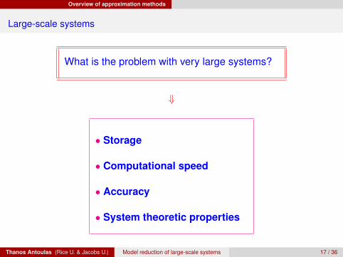
Large-scale systems
What is the problem with very large systems?
⇓
• Storage
• Computational speed
• Accuracy
• System theoretic properties
Thanos Antoulas (Rice U. & Jacobs U.) Model reduction of large-scale systems 17 / 36
Overview of approximation methods
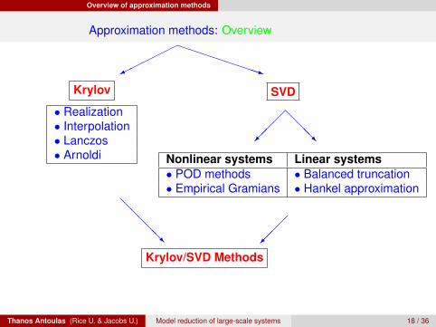
Approximation methods: OverviewPPPPPPPPq
������
Krylov
• Realization• Interpolation• Lanczos• Arnoldi
SVD
@@@R
��
�
Nonlinear systems Linear systems• POD methods • Balanced truncation• Empirical Gramians • Hankel approximation
@@
@@R
���
Krylov/SVD Methods
Thanos Antoulas (Rice U. & Jacobs U.) Model reduction of large-scale systems 18 / 36
Overview of approximation methods SVD
Approximation methods
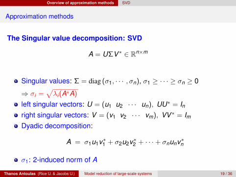
The Singular value decomposition: SVD
A = UΣV ∗ ∈ Rn×m
Singular values: Σ = diag (σ1, · · · , σn), σ1 ≥ · · · ≥ σn ≥ 0
⇒ σi =√
λi(A∗A)
left singular vectors: U = (u1 u2 · · · un), UU∗ = Inright singular vectors: V = (v1 v2 · · · vm), VV ∗ = ImDyadic decomposition:
A = σ1u1v∗1 + σ2u2v∗2 + · · ·+ σnunv∗n
σ1: 2-induced norm of A
Thanos Antoulas (Rice U. & Jacobs U.) Model reduction of large-scale systems 19 / 36

Overview of approximation methods SVD
Reminder: 2-norm
Vectors:
x =
x1...
xn
⇒ ‖ x ‖2 =√
x21 + · · ·+ x2
n
Matrices/Operators: induced 2-norm
A
⇒ ‖ A ‖2 = max‖x‖=1 ‖ Ax ‖2 = σ1
Thanos Antoulas (Rice U. & Jacobs U.) Model reduction of large-scale systems 20 / 36

Overview of approximation methods SVD
Optimal approximation in the 2-norm
Given: A ∈ Rn×m
find: X ∈ Rn×m, rank X = k < rank ACriterion: norm(error) is minimized, whereerror: E = A− X , norm: 2-norm
Theorem (Schmidt-Mirsky, Eckart-Young)
minrankX≤k
‖ A− X ‖2 = σk+1(A)
Minimizer (non-unique): truncation of dyadic decomposition of A:
X# = σ1u1v∗1 + σ2u2v∗2 + · · ·σkukv∗k
Thanos Antoulas (Rice U. & Jacobs U.) Model reduction of large-scale systems 21 / 36
Overview of approximation methods SVD
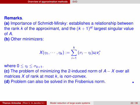
Remarks.(a) Importance of Schmidt-Mirsky: establishes a relationship betweenthe rank k of the approximant, and the (k + 1)st largest singular valueof A.(b) Other minimizers:
X (η1, · · · , ηk ) :=k∑
i=1
(σi − ηi)uiv∗i
where 0 ≤ ηi ≤ σk+1.(c) The problem of minimizing the 2-induced norm of A− X over allmatrices X of rank at most k , is non-convex.(d) Problem can also be solved in the Frobenius norm.
Thanos Antoulas (Rice U. & Jacobs U.) Model reduction of large-scale systems 22 / 36

Overview of approximation methods SVD
SVD Approximation methods
A prototype approximation problem – the SVD(Singular Value Decomposition): A = UΣV∗.Supernova Clown
0.5 1 1.5 2 2.5
−5
−4
−3
−2
−1
Singular values of Clown and Supernova Supernova: original picture
Supernova: rank 6 approximation Supernova: rank 20 approximation
green: clownred: supernova(log−log scale)
Clown: original picture Clown: rank 6 approximation
Clown: rank 12 approximation Clown: rank 20 approximation
Singular values provide trade-off between accuracy and complexity
Thanos Antoulas (Rice U. & Jacobs U.) Model reduction of large-scale systems 23 / 36

Overview of approximation methods POD
POD: Proper Orthogonal Decomposition
Consider: x(t) = f(x(t), u(t)), y(t) = h(x(t), u(t)).Snapshots of the state:
X = [x(t1) x(t2) · · · x(tN)] ∈ Rn×N
SVD: X = UΣV∗ ≈ UkΣk V∗k , k � n. Approximate the state:
x(t) = U∗k x(t) ⇒ x(t) ≈ Uk x(t), x(t) ∈ Rk
Project state and output equations. Reduced order system:
˙x(t) = U∗k f(Uk x(t), u(t)), y(t) = h(Uk x(t), u(t))
⇒ x(t) evolves in a low-dimensional space.
Issues with POD:(a) Choice of snapshots, (b) singular values not I/O invariants.
Thanos Antoulas (Rice U. & Jacobs U.) Model reduction of large-scale systems 24 / 36
Overview of approximation methods Balanced truncation
SVD methods: balanced truncation
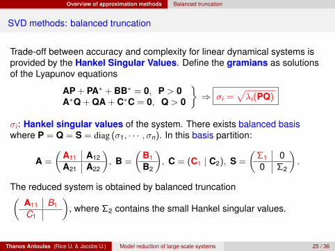
Trade-off between accuracy and complexity for linear dynamical systems isprovided by the Hankel Singular Values. Define the gramians as solutionsof the Lyapunov equations
AP + PA∗ + BB∗ = 0, P > 0A∗Q + QA + C∗C = 0, Q > 0
}⇒ σi =
√λi(PQ)
σi : Hankel singular values of the system. There exists balanced basiswhere P = Q = S = diag (σ1, · · · , σn). In this basis partition:
A =
(A11 A12
A21 A22
), B =
(B1
B2
), C = (C1 | C2), S =
(Σ1 00 Σ2
).
The reduced system is obtained by balanced truncation(A11 B1
C1
), where Σ2 contains the small Hankel singular values.
Thanos Antoulas (Rice U. & Jacobs U.) Model reduction of large-scale systems 25 / 36
Overview of approximation methods Balanced truncation
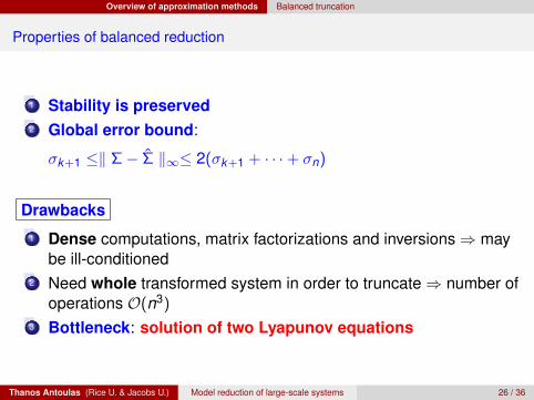
Properties of balanced reduction
1 Stability is preserved2 Global error bound:
σk+1 ≤‖ Σ− Σ ‖∞≤ 2(σk+1 + · · ·+ σn)
Drawbacks
1 Dense computations, matrix factorizations and inversions ⇒ maybe ill-conditioned
2 Need whole transformed system in order to truncate ⇒ number ofoperations O(n3)
3 Bottleneck: solution of two Lyapunov equations
Thanos Antoulas (Rice U. & Jacobs U.) Model reduction of large-scale systems 26 / 36

Overview of approximation methods Krylov methods
Approximation methods: Krylov methodsPPPPPPPPq
������
Krylov
• Realization• Interpolation• Lanczos• Arnoldi
SVD
@@@R
��
�
Nonlinear systems Linear systems• POD methods • Balanced truncation• Empirical Gramians • Hankel approximation
@@
@@R
���
Krylov/SVD Methods
Thanos Antoulas (Rice U. & Jacobs U.) Model reduction of large-scale systems 27 / 36

Overview of approximation methods Krylov methods
The basic Krylov iteration
Given A ∈ Rn×n and b ∈ Rn, let v1 = b‖b‖ . At the k th step:
AVk = Vk Hk + fk e∗k where
ek ∈ Rk : canonical unit vectorVk = [v1 · · · vk ] ∈ Rk×k , V∗v Vk = IkHk = V∗k AVk ∈ Rk×k
⇒ vk+1 = fk‖fk‖ ∈ Rn
Computational complexity for k steps: O(n2k); storage O(nk).
The Lanczos and the Arnoldi algorithms result.
The Krylov iteration involves the subspace Rk =[b, Ab, · · · , Ak−1b
].
• Arnoldi iteration ⇒ arbitrary A ⇒ Hk upper Hessenberg.• Symmetric (one-sided) Lanczos iteration ⇒ symmetric A = A∗
⇒ Hk tridiagonal and symmetric.• Two-sided Lanczos iteration with two starting vectors b, c
⇒ arbitrary A ⇒ Hk tridiagonal.Thanos Antoulas (Rice U. & Jacobs U.) Model reduction of large-scale systems 28 / 36

Overview of approximation methods Krylov methods
Three uses of the Krylov iteration
(1) Iterative solution of Ax = b: approximate the solution x iteratively.
(2) Iterative approximation of the eigenvalues of A. In this case b is not fixedapriori. The eigenvalues of the projected Hk approximate the dominanteigenvalues of A.
(3) Approximation of linear systems by moment matriching.
⇒ Item (3) is of interest in the present context.
Thanos Antoulas (Rice U. & Jacobs U.) Model reduction of large-scale systems 29 / 36

Overview of approximation methods Moment matching
Approximation by moment matching
Given Ex(t) = Ax(t) + Bu(t), y(t) = Cx(t) + Du(t), expand transfer functionaround s0:
G(s) = η0 + η1(s − s0) + η2(s − s0)2 + η3(s − s0)
3 + · · ·
Moments at s0: ηj .
Find E ˙x(t) = Ax(t) + Bu(t), y(t) = Cx(t) + Du(t), with
G(s) = η0 + η1(s − s0) + η2(s − s0)2 + η3(s − s0)
3 + · · ·
such that for appropriate s0 and `:
ηj = ηj , j = 1, 2, · · · , `
Thanos Antoulas (Rice U. & Jacobs U.) Model reduction of large-scale systems 30 / 36
Overview of approximation methods Moment matching
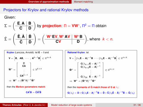
Projectors for Krylov and rational Krylov methods
Given:
Σ =
(E, A BC D
)by projection: Π = VW∗, Π2 = Π obtain
Σ =
(E, A BC D
)=
(W∗EV, W∗AV W∗B
CV D
), where k < n.
Krylov (Lanczos, Arnoldi): let E = I and
V =[B, AB, · · · , Ak−1B
]∈ Rn×k
W∗ =
C
CA...
CAk−1
∈ Rk×n
⇒ W∗ = (W∗V)−1W∗
then the Markov parameters match:
CAiB = CAiB
Rational Krylov: let
V =[(λ1E− A)−1B · · · (λk E− A)−1B
]∈ Rn×k
W∗ =
C(λk+1E− A)−1
C(λk+2E− A)−1
.
.
.C(λ2k E− A)−1
∈ Rk×n
⇒ W∗ = (W∗V)−1W∗
then the moments of G match those of G at λi :
G(λi) = D+C(λiE−A)−1B = D+ C(λiE− A)−1B = G(λi)
Thanos Antoulas (Rice U. & Jacobs U.) Model reduction of large-scale systems 31 / 36

Overview of approximation methods Moment matching
Properties of Krylov methods
(a) Number of operations: O(kn2) or O(k2n) vs. O(n3) ⇒ efficiency
(b) Only matrix-vector multiplications are required. No matrix factorizationsand/or inversions. No need to compute transformed model and then truncate.
(c) Drawbacks
• global error bound?• Σ may not be stable.
Q: How to choose the projection points?
Thanos Antoulas (Rice U. & Jacobs U.) Model reduction of large-scale systems 32 / 36

Summary – Challenges – References
Outline
1 Introduction and model reduction problemThe big pictureProblem formulationProjections
2 Motivating examples
3 Overview of approximation methodsSVDPODBalanced truncationKrylov methodsMoment matching
4 Summary – Challenges – References
Thanos Antoulas (Rice U. & Jacobs U.) Model reduction of large-scale systems 33 / 36

Summary – Challenges – References
Approximation methods: SummaryPPPPPPPPq
������
Krylov
• Realization• Interpolation• Lanczos• Arnoldi
SVD
@@@R
��
�
Nonlinear systems Linear systems• POD methods • Balanced truncation• Empirical Gramians • Hankel approximation@
@@
@R�
��
Krylov/SVD Methods
��
r@
@R
rProperties
• numerical efficiency
• n � 103
• choice of matching moments
Properties
• Stability
• Error bound
• n ≈ 103
Thanos Antoulas (Rice U. & Jacobs U.) Model reduction of large-scale systems 34 / 36
Summary – Challenges – References
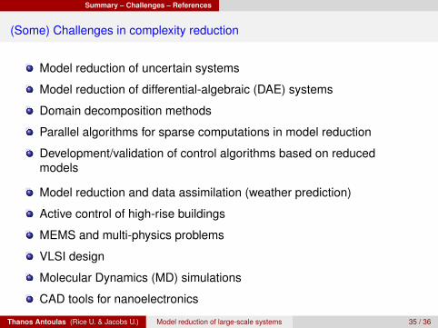
(Some) Challenges in complexity reduction
Model reduction of uncertain systems
Model reduction of differential-algebraic (DAE) systems
Domain decomposition methods
Parallel algorithms for sparse computations in model reduction
Development/validation of control algorithms based on reducedmodels
Model reduction and data assimilation (weather prediction)
Active control of high-rise buildings
MEMS and multi-physics problems
VLSI design
Molecular Dynamics (MD) simulations
CAD tools for nanoelectronics
Thanos Antoulas (Rice U. & Jacobs U.) Model reduction of large-scale systems 35 / 36

Summary – Challenges – References
References
Passivity preserving model reductionAntoulas SCL (2005)Sorensen SCL (2005)Ionutiu, Rommes, Antoulas IEEE TCAD (2008)
Optimal H2 model reductionGugercin, Antoulas, Beattie SIMAX (2008)
Low-rank solutions of Lyapunov equationsGugercin, Sorensen, Antoulas, Numerical Algorithms (2003)Sorensen (2006)
Model reduction from dataMayo, Antoulas LAA (2007)Lefteriu, Antoulas, Tech. Report (2008)
General reference: Antoulas, SIAM (2005)
Thanos Antoulas (Rice U. & Jacobs U.) Model reduction of large-scale systems 36 / 36
Top Related