


Languages
Pages
Legal


Mixed Mimetic Spectral Elements for Geophysical FluidDynamics
Dave Lee
Los Alamos National Laboratory
Lee; LA-UR-17-24044 Mixed Mimetic Spectral Elements
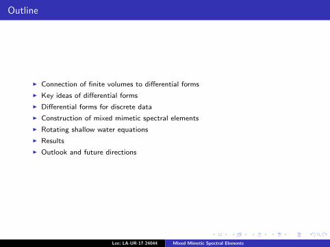
Outline
I Connection of finite volumes to differential forms
I Key ideas of differential forms
I Differential forms for discrete data
I Construction of mixed mimetic spectral elements
I Rotating shallow water equations
I Results
I Outlook and future directions
Lee; LA-UR-17-24044 Mixed Mimetic Spectral Elements
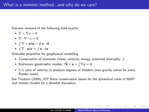
What is a mimetic method...and why do we care?
Discrete versions of the following hold exactly
I ∇×∇φ = 0
I ∇ · ∇⊥ψ = 0
I∫∇× uda =
∮u · dl
I∫∇ · udv =
∫u · da
Desirable properties for geophysical modelling
I Conservation of moments (mass, vorticity, energy, potential enstrophy...)
I Stationary geostrophic modes: f k× u + 1ρ∇p = 0
I 2/1 ratio of velocity to pressure degrees of freedom (two gravity waves for everyRossby wave)
See Thuburn (2008) JCP Some conservation issues for the dynamical cores of NWPand climate models for a detailed discussion
Lee; LA-UR-17-24044 Mixed Mimetic Spectral Elements
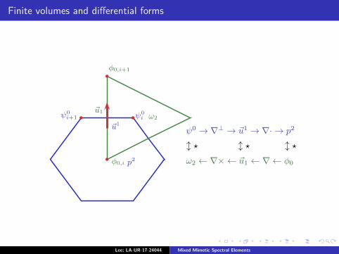
Finite volumes and differential forms
b
b
ω2ψ0i
~u1
~u1
p2φ0,i
ψ0 → ∇⊥ → ~u1 → ∇· → p2
ω2 ← ∇× ← ~u1 ← ∇← φ0
l ⋆ l ⋆ l ⋆
b
bψ0i+1
φ0,i+1
Lee; LA-UR-17-24044 Mixed Mimetic Spectral Elements
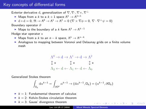
Key concepts of differential forms
Exterior derivative d, generalization of ∇,∇·,∇×,∇⊥I Maps from a k to a k + 1 space Λk → Λk+1
I d d = 0, R→ Λ0 → Λ1 → Λ2 = 0 (∇×∇φ = 0, ∇ · ∇⊥ψ = 0)
Boundary operator ∂I Maps to the boundary of a k form Λk → Λk−1
Hodge star operator ?I Maps from a k to an n − k space, Λk → Λn−k
I Analogous to mapping between Voronoi and Delaunay grids on a finite volumemesh
Λ0 → d→ Λ1 → d→ Λ2
Λ2 ← d← Λ1 ← d← Λ0
l ⋆ l ⋆ l ⋆
Generalized Stokes theorem∫Ωk
dαk−1 =
∫∂Ωk
αk−1 → (dαk−1,Ωk ) = (αk−1, ∂Ωk )
I k = 1: Fundamental theorem of calculusI k = 2: Kelvin-Stokes circulation theoremI k = 3: Gauss’ divergence theorem
Lee; LA-UR-17-24044 Mixed Mimetic Spectral Elements

Application to spectral elements
I The standard (0 form) spectral element basis is given as f 0(ξ) = a0i li (ξ)
I Start from the premise that in 1D we wish to exactly satisfy the fundamental th.of calculus between nodes ξi and ξi+1:∫ ξi+1
ξi
df 0(ξ) = f 0(ξi+1)− f 0(ξi ) = a0i+1 − a0
i = b1i =
∫ ξi+1
ξi
g1(ξ)
I The corresponding 1 form edge function expansion is then given asg1(ξ) = b1
i ei (ξ) subject to
df 0 = g1
I Edge functions are orthogonal with respect to the set of 1 forms such that∫ ξi+1
ξi
ej (ξ) = δi,j
I Satisfies the Kelvin-Stokes and Gauss-divergence theorems in higher dimensionsvia tensor product combinations of li (ξ) and ej (ξ)
Lee; LA-UR-17-24044 Mixed Mimetic Spectral Elements
Algebraic topology and the discrete exterior derivative
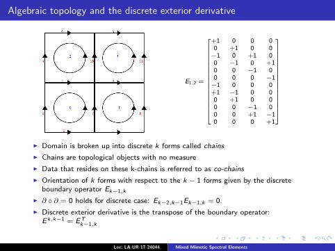
E1,2 =
+1 0 0 00 +1 0 0−1 0 +1 00 −1 0 +10 0 −1 00 0 0 −1−1 0 0 0+1 −1 0 00 +1 0 00 0 −1 00 0 +1 −10 0 0 +1
I Domain is broken up into discrete k forms called chains
I Chains are topological objects with no measure
I Data that resides on these k-chains is referred to as co-chains
I Orientation of k forms with respect to the k − 1 forms given by the discreteboundary operator Ek−1,k
I ∂ ∂ = 0 holds for discrete case: Ek−2,k−1Ek−1,k = 0.
I Discrete exterior derivative is the transpose of the boundary operator:E k,k−1 = ET
k−1,k
Lee; LA-UR-17-24044 Mixed Mimetic Spectral Elements

Example: 1D wave equation
∂p1
∂t= −du0 ∂u0
∂t= −d ? p1
Discretize velocity (0-form) and pressure (1-form) within each element
u0(ξi ) = lj (ξi )u0j = Mi,ju
0j p1(ξi ) = ej (ξi )p
1j = Ni,jp
1j
First equation may be solved in the strong form as
dp1i
dt= −du0
j
= −E1,0i,j u
0j
= −(u0j+1 − u0
j )
Second equation may be solved in the weak form via the adjoint relation
d
dt(la, lb)Ωk
u0b = −(la, d ? ec )Ωk
p1c
= (dla, ec )Ωkp1c + B.C .s
= E0,1,a,d (ed , ec )Ωkp1c + B.C .s
Lee; LA-UR-17-24044 Mixed Mimetic Spectral Elements
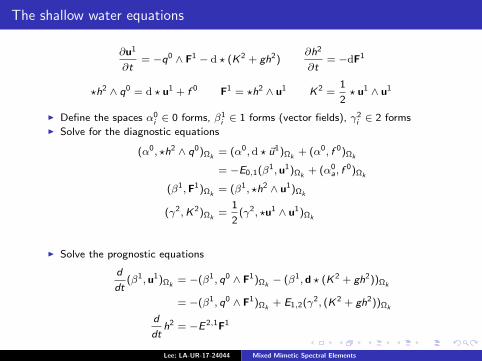
The shallow water equations
∂u1
∂t= −q0 ∧ F1 − d ? (K2 + gh2)
∂h2
∂t= −dF1
?h2 ∧ q0 = d ? u1 + f 0 F1 = ?h2 ∧ u1 K2 =1
2? u1 ∧ u1
I Define the spaces α0i ∈ 0 forms, β1
i ∈ 1 forms (vector fields), γ2i ∈ 2 forms
I Solve for the diagnostic equations
(α0, ?h2 ∧ q0)Ωk= (α0, d ? ~u1)Ωk
+ (α0, f 0)Ωk
= −E0,1(β1, u1)Ωk+ (α0
a, f0)Ωk
(β1,F1)Ωk= (β1, ?h2 ∧ u1)Ωk
(γ2,K2)Ωk=
1
2(γ2, ?u1 ∧ u1)Ωk
I Solve the prognostic equations
d
dt(β1, u1)Ωk
= −(β1, q0 ∧ F1)Ωk− (β1, d ? (K2 + gh2))Ωk
= −(β1, q0 ∧ F1)Ωk+ E1,2(γ2, (K2 + gh2))Ωk
d
dth2 = −E2,1F1
Lee; LA-UR-17-24044 Mixed Mimetic Spectral Elements
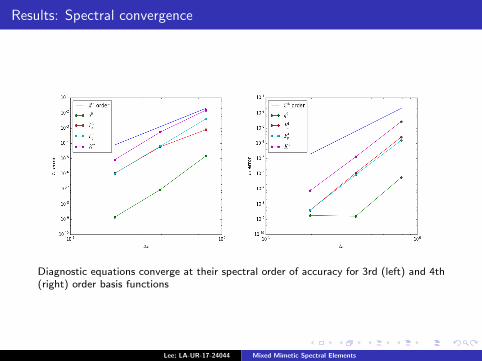
Results: Spectral convergence
Diagnostic equations converge at their spectral order of accuracy for 3rd (left) and 4th(right) order basis functions
Lee; LA-UR-17-24044 Mixed Mimetic Spectral Elements
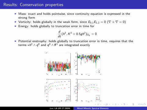
Results: Conservation properties
I Mass: exact and holds pointwise, since continuity equation is expressed in thestrong form
I Vorticity: holds globally in the weak form, since E0,1E1,2 = 0 (∇×∇ = 0)I Energy: holds globally to truncation error in time for
d
dt(h2,K2 + 0.5gh2)Ωk
= 0
I Potential enstrophy: holds globally to truncation error in time, requires that theterms ?h2 ∧ q0 and q0 ∧ F1 are integrated exactly
Lee; LA-UR-17-24044 Mixed Mimetic Spectral Elements
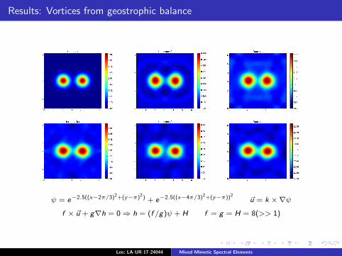
Results: Vortices from geostrophic balance
ψ = e−2.5((x−2π/3)2+(y−π)2) + e−2.5((x−4π/3)2+(y−π))2~u = k ×∇ψ
f × ~u + g∇h = 0⇒ h = (f /g)ψ + H f = g = H = 8(>> 1)
Lee; LA-UR-17-24044 Mixed Mimetic Spectral Elements
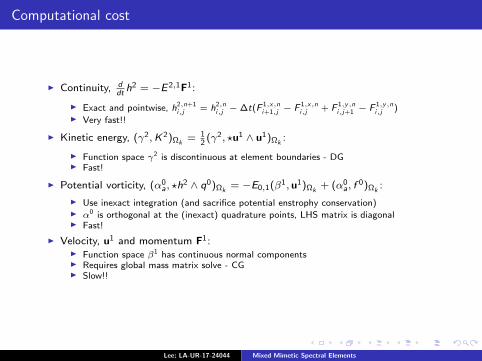
Computational cost
I Continuity, ddth2 = −E2,1F1:
I Exact and pointwise, h2,n+1i,j = h2,n
i,j − ∆t(F 1,x,ni+1,j − F 1,x,n
i,j + F 1,y,ni,j+1 − F 1,y,n
i,j )I Very fast!!
I Kinetic energy, (γ2,K2)Ωk= 1
2(γ2, ?u1 ∧ u1)Ωk
:
I Function space γ2 is discontinuous at element boundaries - DGI Fast!
I Potential vorticity, (α0a, ?h
2 ∧ q0)Ωk= −E0,1(β1, u1)Ωk
+ (α0a, f
0)Ωk:
I Use inexact integration (and sacrifice potential enstrophy conservation)I α0 is orthogonal at the (inexact) quadrature points, LHS matrix is diagonalI Fast!
I Velocity, u1 and momentum F1:I Function space β1 has continuous normal componentsI Requires global mass matrix solve - CGI Slow!!
Lee; LA-UR-17-24044 Mixed Mimetic Spectral Elements
Outlook
I Can we get exact conservation of energy independent of time step viasemi-implicit, staggered time stepping as has been done for Navier Stokes?[Palha and Gerritsma, (2017), JCP]
I Should we be prognosing the vorticity rather than diagnosing?
I Can we do this on the sphere via isoparametric mapping from computationaldomain? - Should be ok since volume, vorticity and energy conservation hold forinexact integration.
I Conservation of potential vorticity requires exact integration - can we do this withinexact integration? - do we even care?
I Turbulence closure: Anticipated Potential Vorticity Method, dissipates enstrophybut preserves energy conservation [Sadourny and Basdevant, (1985), JAS].
Lee; LA-UR-17-24044 Mixed Mimetic Spectral Elements
References
Geostrophically balanced finite volumes:
I Thuburn, Ringler, Skamarock and Klemp (2010) JCP
I Ringler, Thuburn, Klemp and Skamarock (2010) JCP
I Peixoto (2016), JCP
Mimetic finite elements for geophysical flows:
I Cotter and Shipton (2012) JCP
I Cotter and Thuburn (2014) JCP
I McRae and Cotter (2014) QJRMS
I Thuburn and Cotter (2015) JCP
Spectral elements (a-grid):
I Taylor and Fournier (2010) JCP
I Melvin, Staniforth and Thuburn (2012) QJRMS
Mixed spectral elements:
I Palha and Gerritsma (2011) Spectral and High Order Methods for PartialDifferential Equations
I Kreeft and Gerritsma (2013) JCP
I Palha, Rebelo and Gerritsma (2013) Mimetic Spectral Element Advection
I Hiemstra, Toshniwal, Huijsmans and Gerritsma (2014) JCP
Lee; LA-UR-17-24044 Mixed Mimetic Spectral Elements
Top Related