


Languages
Pages
Legal


MIT OpenCourseWare http://ocw.mit.edu
Haus, Hermann A., and James R. Melcher. Solutions Manual for Electromagnetic Fields and Energy. (Massachusetts Institute of Technology: MIT OpenCourseWare). http://ocw.mit.edu (accessed MM DD, YYYY). License: Creative Commons Attribution-NonCommercial-Share Alike. Also available from Prentice-Hall: Englewood Cliffs, NJ, 1990. ISBN: 9780132489805. For more information about citing these materials or our Terms of Use, visit: http://ocw.mit.edu/terms.

SOLUTIONS TO CHAPTER 12
12.1 ELECTRODYNAMIC FIELDS AND POTENTIALS
12.1.1 The particular part of the E-field obeys
Hwe set
then
or
Because of (2),
a v x Ep = -atB (1)
v .EoEp = 0 (2)
B=VxA (3)
v x (Ep + aa~) = 0 (4)
Ep = a
- atA V.p (5)
a 2at v .A + V .p = 0 (6)
But, because we use the Coulomb gauge,
V·A=O (7)
and thus V2 • p = 0 (8)
There is no source for the scalar potential of the particular solution. Further
(9)
Conversely, (10)
and v X E,. = 0 (11)
Therefore, E,. = -V.,. (12)
and from (10)
(13)
Thus (9) and (13) look like the inhomogeneous wave equation with a2 jat2 terms omitted.
1

12-2 Solutions to Chapter 12
12.1.2 %t22 A is of order l/r2A, V2A is of order A/£2. Thus, J1.f.%t22 A is of order '!f£2
compared with V 2A. It is negligible if J1.f.£2 /r2 = £2 /c2r2 ~ 1. The same approachshows that J1.f.(a2/at2)cp can be neglected compared with V 2 CP if £2 /c2r2 ~ 1.
12.2 ELECTRODYNAMIC FIELDS OF SOURCESINGULARITIES
12.2.1 The time dependence of q(t) is the same as that of Fig. 12.2.5, except that itnow extends over one full period.
t = 1'/2
t T rq( - - -)
-- 2 0 t .T r--, q(---)-,- - / 2 0
~ , " ,/' ......... "
-,\\
\ ," "
t = l'
," '
'---~ ql(T-~)o
/ "l-(---"I'l"_ ," I I 1\
---r
E-Iine.
~
//
/
'"
E-Iine.
Figure S12.2.1a
Plot of Electric Dipole Field. Any set of field lines that close upon themselves
-----
12-3 Solutions to Chapter 12
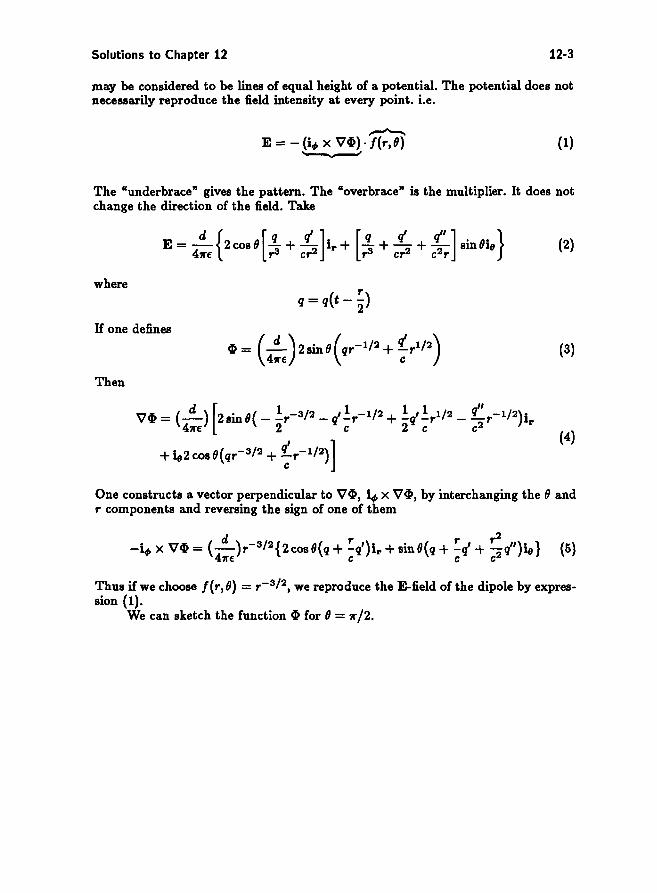
may be considered to be lines of equal height of a potential. The potential does not necessarily reproduce the field intensity at every point. i.e.
........-...E = - (i<l> X V~). f(r,9) (1)
The "underbrace" gives the pattern. The "overbrace" is the multiplier. It does not change the direction of the field. Take
II [ r/ ]'I .. + + 2r/ sm ll'ul8E= -d{2 3"q + 2 [ _qq +""2q"]. } (2)cos u 411"E r cr r cr c r
where q = q(t - .!:.)
2
IT one defines
(3)
Then
V~ = (~) [2 sin 9( - !r-3/ 2 - q' !r-1/ 2 + !r/!r1/ 2 _ r/' r- 1/ 2)i.. 411"E 2 c 2 C c2
(4) + ie2 cos 9(qr-3
/ 2 + ~ r- 1
/ 2
) ]
One constructs a vector perpendicular to V~, i<l> X V~, by interchanging the 9 and r components and reversing the sign of one of them
Thus if we choose f(r, 9) = r-3/ 2 , we reproduce the E-field ofthe dipole by expression (1).
We can sketch the function ~ for 9 = 11"/2.

12-4 Solutions to Chapter 12
t=2T
(J
,.-- .....'" ... -/ "."<"
" , '.... '.- "' ...
/P-t,/( I I 1,
.... - -,' I I II I II I II I II I I
I
Figure SU.J.lb
12.2.2 Interchange E - H, H - -E and 1'0 - Eo. From (23)
di = iwqd - iwqmd = iWlJom (l)
where qm is the magnetic charge. We obtain
Ok.. 0" -;1cr1 1wIJom • lieE4> = - smu-- (2)411" r
T rq'(---)
2 c
-r

Solutions to Chapter 12 12-5
and from (24)
QED (3)
12.2.3 Because Io'om(t) = qmd - qd in the electric dipole case, the time dependence of q(t)d and Io'om(t) correspond to each other. With E - H and H - -E we must obtain mutually corresponding field patterns.
12.2.4 We can use the field sketch of Problem 12.2.1 with proper interchange of variables.
12.3 SUPERPOSITION INTEGRAL FOR ELECTRODYNAMIC FIELDS
12.4: ANTENNAE RADIATION FIELDS IN THE SINUSOIDAL STEADY STATE
12.4.1 From (4)
tPo(O) = sin 0 (' e-jlc.' ,:ilc.' cOIBdz'
l 10 = sin 0 1 {e-jlc(1-co8B)' _ I} (I)
I jk(cos 0 - 1)
= sinO 2 . [kl(l_ n)] -jlc(1-co8B)'/2 l k(I-cosun) sm
2 cos u e
The radiation pattern is
(2)
With kl = 271" .T.(n) _ sin
20 (. 2 2 . 2 0)... u = Sln 7I"sm- (3)
471"2 sin4 (Oj2) 2
The radiation pattern peaks near 0 = 60°.
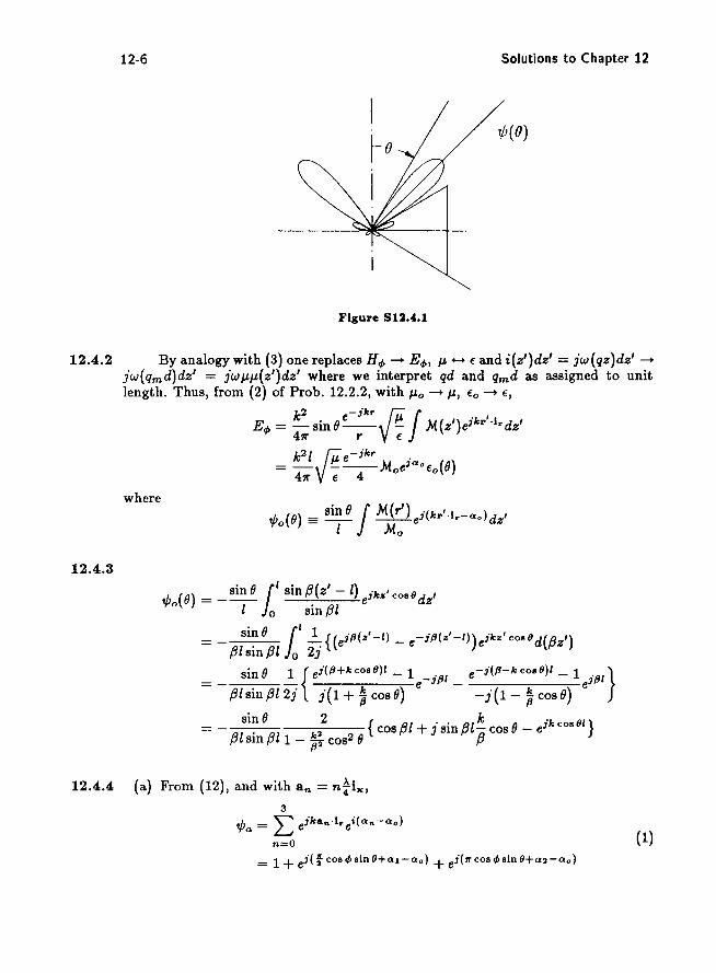
Solutions to Chapter 12 12-6
1jJ(O)
Figure 812.4.1
12.4.2 By analogy with (3) one replaces H<f> - E<f>, IJ +-+ f and i(z')dz' = jw(qz)dz' J'w(qmd) dz' = J'wIJIJ(z')dz' where we interpret qd and qmd as assigned to unit length. Thus, from (2) of Prob. 12.2.2, with IJo - IJ, fo - f,
2 jkr I¥! ., E<f> = -sinO--k e- - M(z')eJkr'lrdz'4'11' r f
2 jkr = k I . ~e- M ejOl.°f (0)
4'11' V~ 4 0 0
where
12.4.3
tPo(O) = _sinO (' sin~(z' -I) ejkz'cos8dz'I Jo sm {3I
= _ si~O {' ~{(ej~(z'-I) _ e-j~(z'-I))ejkzlcOs8d({3z') {3lsm{3I Jo 2J
sinO 1 {ej (IJ+kCOS8)1 -1 _. I e-j (IJ-kcos8)1 -1 e3IJ
. ,}= - - e J~
(3lsin{3I2j j(l+~cosO) -j(l-~cosO)
sin 0 2 {{3I' . {3I k jk cos 81}= {31' {3I k 2 cos + J sm -(3 cos 0 - e
sm 1- "ji'i cos2 0
12.4.4 (a) From (12), and with an = n~ix,
tPa = L3 ejka".lrei(OI.,,-OI.o)
(1)n=O
= 1 + ej(f cos <f> sin 8+01.1-01. 0 ) + ej (7I' cos <f>sin 8+01.2-01. 0 )

12-7 Solutions to Chapter 12
(b) Since tPo = sin 0, and Qi = 0
ItPolltPal = 11 + 2 cos (i cos e; sin 0) IsinO (2)
(c) tPa = 1 + ejf(C08~8iD9+1) + ejll'(Co8~8in9+1)
= ejf(Co8~8in9+1){e-jf(c08~8iD9+1) + 1+ ejf(C08~8iD9+1)} (3)
= ejf(Co8~8in 9+1) [2 cos i(cos e; sin 0+ 1) + 1]
12.4.5 (a)
tPa(O) = L1
ejlc....lrej(a .. -ao) = 1+ e j [lI'co8/1+al- a o] (1) n=O
(b) (2)
(c) G = 411"cos2 (~cosO) sin2 0
I; dO 1:11' de; sin 0cos2 (~cos 0) sin2 0 (3)
Define cosO = u (4)
r dO sin3 0cos2 (~cos 0) = j1 du(I- u2 ) cos2 (~u) (5)Jo 2 -1 2
Now consider integral
I d 2 2 1 ( 1. 2 ) 2 z3 2z 1 . zz cos "z = '2 z + '2 sm z z - 3" + "8 cos 2z - 8" sm 2% (6)
The integral is
Solutions to Chapter 12 12-8
The gain is 411'" cos2 (~ cos 0) sin2 0
G - ---7~-;:;''-;:-- (8) - 211'"U + ;2}
(d) We find for '11(0) of array
'11(0) = {I1/10(0) I11/11(0)111/12(0)1}2 (9)
with 1/12(0) = 1- eikasinOcos'" (10)
In order to get maximum superposition in the direction 4> = 0, one needs ka = 11'" or a = >../2. Thus
11/12(0) I= 12 sin (~sin 0 cos 4» I
12.5 COMPLEX POYNTING'S THEOREM AND RADIATION RESISTANCE
12.5.1 The radiation field Poynting vector of the antenna is from 12.4.2, 3.4.5
~(EoH;) = ~ ((:~): filloI2(1/Io(0))2 (1)
where 1/10(0) is from 12.4.28
_ 1 cos ( 3;) - cos (3; cos 0) 1/10(0) - e1\') . e1\') . 0""2 sm ""2 sm (2)
~ cos (~cosO) 311'" sin 0
The radiated power is
2 ~1 1\' 121\' 1 ~-110 1Rrad = dO sin 0 d4>-EoH;2 10 0 2
_ ! (311'")2. ~/ II 12(~)2 11\' cos2(~cosO) . (3)- 2 (4 )2 V J.Lo/ fa a 3 211'" . 2 sm OdO11'" 11'" 0 sm 11
= !II 12 VJ.Lo/fo( )l1\'dO' cos2 e; cosO)
a 2 211'" smO 2 2 411'" 0 sin 0
ThereforeVJ.LO/fO11\' . cos2(3; cos 0)
Rrad = 2 dO sm 0 . 2 11'" 0 sm 0
_ 1 11 cos2(321\' x) (4)- -VJ.Lo/fo dx 2211'" -1 1- x
= 1040

Solutions to Chapter 12 12-9
12.5.2 The scalar potential of the spherical coil is (see Eq. 8.5.17)
(1)
This identifies
(2)
We have for the 0 component of the H-field
(3)
and thus the radiation field is
k2 A
A mHo ~ ---sinO
411"r (4)
The power radiated is
(5)
Therefore,
Rrad = ~; VlLo/foN 2 (kR)4 (6)
The inductance of the coil is from (8.5.20)
(7)
and therefore
(8)
12.6 PERIODIC SHEET-SOURCE FIELDS: UNIFORM AND NONUNIFORM PLANE WAVES
Solutions to Chapter 12 12-10
12.6.1 (a) From continuity:
ak:c . A 0 az + 3wO'. =
Taking into account the z-dependence:
(2)
and therefore (3)
and
(b) The boundary condition on the tangential B is:
nil I)'
Since B II i. (4)
and thus b: - b: = k:c (5)
H. is antisymmetric, of opposite sign on the two sides of current sheet.
(6)
and thus
(7)
From (12.6.6) and (12.6.7)
E = Re[ix ( - f30'0) + i)'( ± 0'0 )]e'Fillllei(wt-k.,:c) (8) 2Eok:c 2Eo
(c) As in Problem 12.2.1, a plot of a divergence-free field can be done by defining a potential. and obtaining the field
(9)
Now, it is clear that the potential necessary to produce (8) is

12-11 Solutions to Chapter 12
Then • ~;o,. • 8q, • 8q,
-I" X v 'li' = Ix 8y - I)' 8x
and is found to be equal to (8) with f(x, y) equal to unity. By visualizing the potential, one may plot E lines.
k y imaginary: H-lines E-lines
lines of equal height of ~
Figure S12.6.1a
At wt = 0, the potential is
k y real:
E-line
../ H-line
L
Figure S12.6.1b
x

Solutions to Chapter 1212-12
At wt = 0, the potential is
12.6.2 (a) The E-field will be z-directed, the H-field is in the z - y plane
t. = Asin(kzz)e'fi1c1l1l (1)
From (12.6.29)
I'r 1 8E. 1 ( ·k)A· kn z = --.--- = --.- T' SIB zZ (2)'WIJ 8y ,wIJ II
The discontinuity of tangential H gives:
D X (DB - Db) = K (3)
in z - z plane. And thus, combining (2) and (3)
(4)
and therefore A=_wIJKo (5)
2lell
From (2) and (5)
(6)
and from (12.6.30)
II II
= ,.lek z K
2 o cos(k
z z)e'fi1c1l1l (7)
II
(b) Again we can use a potential ~ to which the H lines are lines of equal height. IT we postulate
Then
~ = (~) Ko sink ze'fi1c1l1likll 2 z
• VA;. • 8~ Ko kz k -I. X '* = Ix 8y T ik cos zZ
ll
• 8~ • K o • k • Ko kz -I)" 8z = TlxT SIB zZ -I)" T ik cos
ll
The potential hill at wt = 0 is
Re[~J = T~o sin kzz sin klly
(8)
(9)
k zZ
(10)

Solutions to Chapter 12
wt = 0
o 0 0
o
o H-Iine
E-Iine
12-13
oo
(c) We may write (1)
o 0 0
Figure Sn.6.2
and for (6) and (7)
:H: =i Ko { ± ix(eik.."'=fikYI/ _ e-ik.."'=fikyl/)4
+ :'" ill (eik .."'=fikYI/ + e-ik.. "'=fikyl/)}1/
(11)
(12)
12.6.3 (a) At first it is best to find the field E z due to a single current sheet at y = O.We have
From (12.6.29)
(1)
(2)

12-14 Solutions to Chapter 12
From the boundary condition
(3)
we get
2LAe-:iksf/ll = _Ke-:iksf/ll WI-'
and thus A = _ wI-'K (4)
2fJ
Now we can add the fields due to each source
(5)
(b) When
(6)
Then K b = -Kae-j(ltl (7)
there is cancellation at 11 < -d/2 (c)
(8)
(d) In order to produce maximum radiation we want the endfire array situation of fJd = 'If/2. (Indeed, sin fJd = 1 in this case.) Because
(9)
we have1 [ ] 1/2w=-Viii ~_(~)2 (10)
f/Il 2d
The direction is

Solutions to Chapter 12 12-15
12.6.4- (a) If we want cancellations, we again want (compare P12.6.3)
Ub = -ua.e-;klld (1)
(b) A single sheet at y = d/2 gives
H. = ±Ae-;k..ze'F;k ll (lI- t) (2)
Now,akz .,.--+JW(T=O (3)az
gives k
z = kW,.(Ta. (4)
z
and
2h;I II=0+ = ~ (Ta (5)
Therefore A
= 2kW,.
(To. (6) z
and the field of both sheets is
H. = j~ua.e-;k"Ze-;kll(lI+t) sinkzd (7)kz
(c) klld = 11'/2. Therefore, as in P12.6.3,
W = _1_[k2 _ (.!.)2] 1/2..;iiE z 2d
(8)
12.7 ELECTRODYNAMIC FIELDS IN THE PRESENCE OF PERFECT CONDUCTORS
12.7.1 The field of the antenna is that of a current distribution Icoskzl. We may treat it in terms of an array factor of three antennae spaced >../2 apart along the z-axis. From 12.4.12
3
l,pa(O)1 = 1L:e'kt COB91 = 11+eiJrcoB9 +e2;JfCOB91 ,=0 (1)
= le-;JfCOB9 + 1 + e;JfCoB91
= 1+ 2cos (11' cos 0)
The function ,polO) follows from 12.4.8 with kl =11'
,polO) = ! cos (~cos 0)/ sin 0 (2)11' 2
Combining (1) and (2) we complete the proof.

Solutions to Chapter 12 12-16
12.7.2 The current distribution, with image, is proportional to Isin kz I. The point at which the current is fed into the antenna calls for sero current. Since the radiated power is finite, Rrad is infinite. In practice, because of the finite losses, it is not infinite but much larger than VIl-o/Eo.
12.7.3 (a) We have a surface current k z
akz ... az + 1WO'. = 0 (1)
Therefore .. jw. (1l"Z)Kz = -TO'o SID - (2)'II'" a a
The H-field is z-directed and antisymmetric with respect to y.
.. ('II'"z) '/I:HM = ±Asin -. e~' IIY (3)a
From the boundary condition
n x (ila - ilb) = it. (4)
with n II ir-A . (z) jw . (z)2 SID - = --O'oSID - (5)
a 'II'"/a a
jwA= ---0' (6)
2'11'"/a 0
The E-field is from (12.6.6)
t 1 all. 1 ( iw ) . . (z) '/I:z = -.--- = ±-,- - --0'0 (=f1k ) SID - e~' IIY 1WEo ay 1WEo 2'11'"/a Y a
jkyO'o . ('II'"z) ~j/l: y (7)
= Sln-e II Eo(2'11'"/a) a
and from 12.6.7
E 1 all. ( 1)( iWO'o) 'II'" ('ll") '/I:y = --.--- = - -,- =f -- -cos -z e~' II" 1WEo az 1WEo 2('II'"/a) a a (8) 0'0 () '/I:=±-cos -z e~' II"
2100 a
(b) On the plate at z = -a/2
... t I jk"O'o ~'/I:0'. = Eo z z=-a/2 = - 2'11'"/a e ' II" (9)

Solutions to Chapter 12
At z = a/2 it is of opposite sign. The surface current is
~ Ii I - iwuo Tile yA y = - II 11.=-0./2 - ±-/-e 1/2'11" a
and is the negative of that at z = a/2.(c)
k2 k2 2II. + y = W /-&oEo
and thus
12-17
(10)
(11)
(12)ky = VW2 /-&oEo _ {~)2
Again we may identify a potential whose lines of equal height give E. Indeed,
(13)
gives
(14)
(d) For kg imaginary and wt = 0
wt =0 wt = rr/2
displacementcurrent density
Flsure 812.7'.3.

12-18 Solutions to Chapter 12
For kv real, wt = 0
Re[.J ==f sin cr:l:) cos kv!lto/)Eo 211' a a
wt = 0 wt = 71" /7.
disphu:ement
convection current
displacement ftux \Ins
Figure S12.f.lb
12.1.4 (a) We now have a TE field with
(1)
From (12.6.29)
18E16 1 (. (1I':I:)'F'/oIia: = --.--- = --.- =f1k )Acos - e IIV:J 1w~ 8y 1w~ 11 a
(2) = ± k1l A cos (11':1:) e'Fj/ollv
w~ a
Solutions to Chapter 12
and the boundary condition
we obtain relation for A:
k" '11":& '11":&-2-Acos - = Kocos-
wp a a
12-19
(3)
(4)
or
and thus
From (12.6.60)
A= _ wpKo
2k"(5)
(6)
(7)
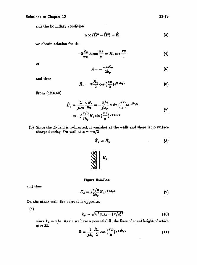
(b) Since the E-field is z-directed, it vanishes at the walls and there is no surfacecharge density. On wall at :& = -a/2
and thus
Flsure SlJ.T.(a
k - .'II"/a K 'fi"~"II - 3 2k oe
"On the other wall, the current is opposite.
(8)
(9)
(c)k" = JW2poEo - ('II"/a)2 (10)
since kill: = 'II"/a. Again we have a potential~, the lines of equal height of whichgive B.
1 Ko ('11":&)",""~ = --cos - e" ~"
jk" 2 a(11)

12-20
(d) For ky imaginary:
wt = 0
Solutions to Chapter 12
wt = 1r/2
,_--..-- H-lield
o ~---r- E-field
00Gx
000
o
Figure SU.f.4b
for ky real:o
Eo 0 ~000
o
00(;)(;) 0 0
o
Figure SU.f.4.:
H
wt =0
Top Related