![Coherent Detection of Turbo-Coded OFDM Signals … · an OFDM frame when it is not present) ... synchronization for OFDM are given in [15]– ... Detection of OFDM signals, ...](https://static.fdocuments.us/doc/165x107/5ae5fd777f8b9a08778c6dfc/coherent-detection-of-turbo-coded-ofdm-signals-ofdm-frame-when-it-is-not-present.jpg)


Languages
Pages
Legal


63
CHAPTER 3
MIMO-OFDM DETECTION
3.1 INTRODUCTION
This chapter discusses various MIMO detection methods and their
performance with CE errors. Based on the fact that the IEEE 802.11n channel
models have high SFCF, a low complexity method of implementing the MIMO-
OFDM detectors is proposed with no significant performance degradation. The
performance analysis is based on simulation which was done for the TGn sync
proposal and with various MIMO detection algorithms. The effect of CE on the
system performance is also studied.
The chapter is organized as follows, the first section discusses the
simple MIMO system model with a flat fading channel between the transmitter
and receiver antenna pair. In section 3.3.2 various MIMO detection methods are
employed for the system model established and the performance of the schemes
are discussed with simulations. Section 3.4 discusses the system model of the
MIMO-OFDM system and a low complexity method of implementing the MIMO
detectors with representative results. In section 3.5, the performance of the TGn
sync system with various CE schemes discussed in chapter 2 is discussed with
various MIMO detectors. Finally the performance of the TGn system in terms of
packet error rate (PER) is obtained by simulations for the low complexity method.
64
3.2 MIMO SYSTEM MODEL
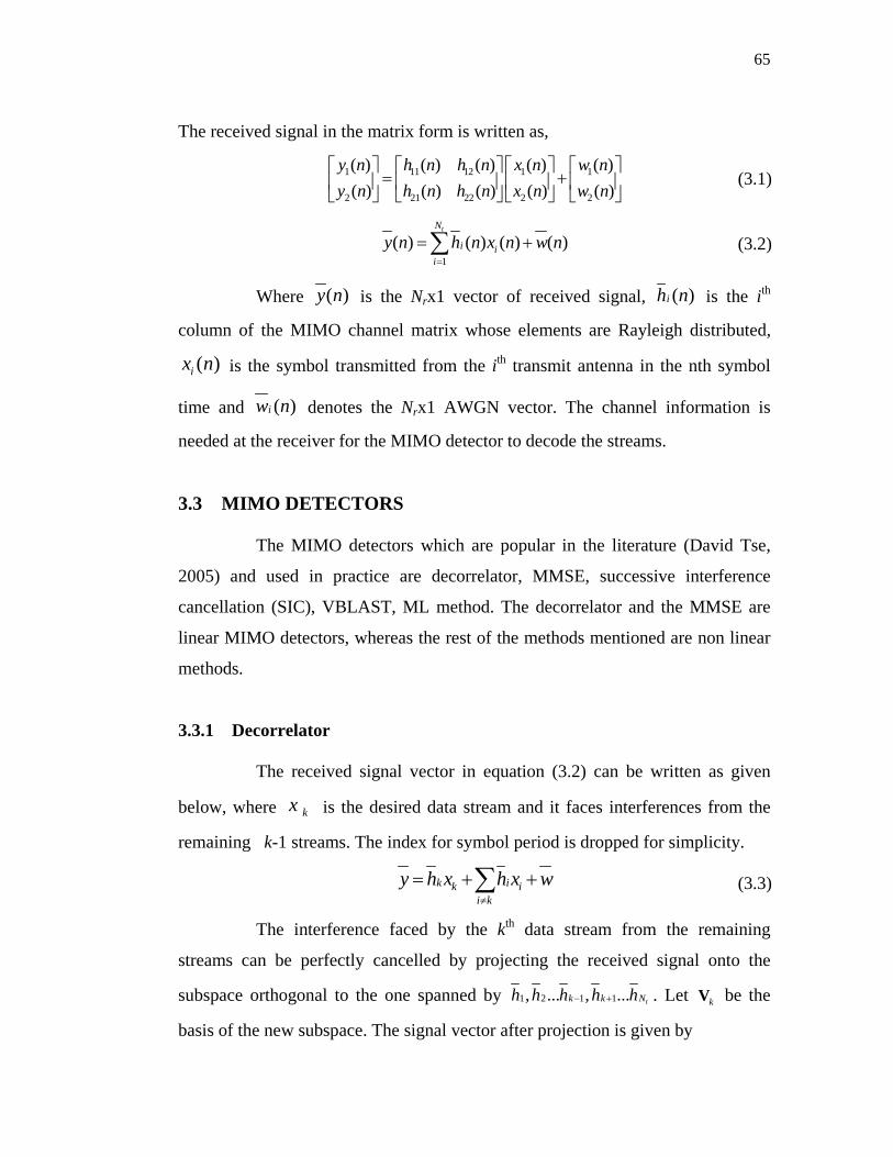
A simple MIMO system model shown in Figure-3.1 is established for
discussing the MIMO detection algorithms and to extend the idea to the MIMO-
OFDM system. In Figure-3.1 a system with Nt transmit and Nr receive antennas is
shown. Let us assume that Nt=Nr=2 as it is the mandatory mode of operation in the
802.11n proposals.
The two streams of incoming bits are modulated to symbols and
transmitted simultaneously from the two antennas. According to the flat fading
channel assumption, there is a single tap between every transmit-receive antenna
pair. The channel taps are Rayleigh distributed and independent of each other. The
AWGN is added at the front end of the receiver. The received signal on the two
antennas are passed into the MIMO detector block, whose function is to separate
out the spatially combined signal transmitted from the multiple antennas, with the
knowledge of the channel coefficients. The output of the MIMO detector block is
passed through the demodulator for obtaining the bits. In these spatial
multiplexing systems, no explicit orgthogonalization or coding is necessary at the
transmitter for signal decorrelation; instead the propagation medium with rich
multipath scattering can be used at the receiver for separating out the spatially
combined transmitted streams (Arogyaswami Paulraj et al, 2003).
MOD
MOD
b1(n)
b2(n)
Demod
MIMO
Detector
Demod
w1
w2
h11
h22
h21
h12
Figure 3.1: A simple 2x2 spatial multiplexing MIMO system
x1(n)
x2(n)
x’1(n)
x’2(n)
b’1(n)
b’2(n)
65
The received signal in the matrix form is written as,
1 11 12 1 1
2 21 22 2 2
( ) ( ) ( ) ( ) ( )( ) ( ) ( ) ( ) ( )
y n h n h n x n w ny n h n h n x n w n⎡ ⎤ ⎡ ⎤ ⎡ ⎤ ⎡ ⎤
= +⎢ ⎥ ⎢ ⎥ ⎢ ⎥ ⎢ ⎥⎣ ⎦ ⎣ ⎦ ⎣ ⎦ ⎣ ⎦
(3.1)
1
( ) ( ) ( ) ( )tN
i ii
y n h n x n w n=
= +∑ (3.2)
Where ( )y n is the Nrx1 vector of received signal, ( )ih n is the ith
column of the MIMO channel matrix whose elements are Rayleigh distributed,
( )ix n is the symbol transmitted from the ith transmit antenna in the nth symbol
time and ( )iw n denotes the Nrx1 AWGN vector. The channel information is
needed at the receiver for the MIMO detector to decode the streams.
3.3 MIMO DETECTORS
The MIMO detectors which are popular in the literature (David Tse,
2005) and used in practice are decorrelator, MMSE, successive interference
cancellation (SIC), VBLAST, ML method. The decorrelator and the MMSE are
linear MIMO detectors, whereas the rest of the methods mentioned are non linear
methods.
3.3.1 Decorrelator
The received signal vector in equation (3.2) can be written as given
below, where kx is the desired data stream and it faces interferences from the
remaining k-1 streams. The index for symbol period is dropped for simplicity.
k ik ii k
y h x h x w≠
= + +∑ (3.3)
The interference faced by the kth data stream from the remaining
streams can be perfectly cancelled by projecting the received signal onto the
subspace orthogonal to the one spanned by 1 2 1 1, ... , ... tk k Nh h h h h− + . Let kV be the
basis of the new subspace. The signal vector after projection is given by
66
' 'kk k ky y h x w= = +V V (3.4)
The demodulation of the kth stream can be performed by match filtering
on the signal to get the unquantized estimate of the data symbol on the kth stream,
,k uqx and quantization is finally applied to obtain data symbol on the kth stream,
kx , which is given below,
( ) ( )
( ),
,
'H H
k uq k k kk k k k
k k uq
x h h x h w
x Q x
= +
=
V V V (3.5)
The combination of projection operation followed by the matched filter
is called the decorrelator or zero forcing (ZF) detector. A simple formula for
demodulating all the streams at once, is given by
† †uqx x w= +H H H (3.6)
where ( ) 1† H H−=H H H H , is the pseudo inverse of H. The ZF detector suffers from
noise enhancement especially in the lower SNR range as it tries to completely null
out the interference without regard to the loss in energy of the desired stream.
3.3.2 Linear MMSE
As we have already discussed, since the decorrelator completely
cancels out the interference, it performs better in higher SNR range. On the other
hand, the matched filtering or maximal ratio combining receiver tries to maximize
the output SNR of the desired stream. The matched filtering receiver performs
well in the lower SNR case where the AWGN is dominant and in the higher SNR
range it suffers from heavy inter-stream interference. Thus, there exists a tradeoff
between completely eliminating the inter-stream interference and preserving as
much energy content of the stream of interest. The linear detector which optimally
combines the decorrelator and the matched filter is the MMSE detector, which is
shown in the Figure-3.2.

67
The objective function of the MMSE MIMO detector is given by,
{ }2 2arg min arg minuqE x x E x w x⎧ ⎫
= − = + −⎨ ⎬⎩ ⎭V V
V VH V (3.7)
Using Wiener-Hopf equation and solving for the optimal solution leads to the
MMSE solution matrix given by
12
2H n
opt mmses
σσ
−⎛ ⎞
= = +⎜ ⎟⎝ ⎠
V V H H H I (3.8)
The data symbols transmitted on all the streams, x is obtained as follows,
( )
12
2
( )
H H Hnuq mmse
s
uq
x y y
x Q x
σσ
−⎛ ⎞
= = +⎜ ⎟⎝ ⎠
=
V H H I H (3.9)
From the MMSE solution matrix given in equation (3.8) it can be
observed that at higher SNR values it is very close to the pseudo inverse of H
matrix, which is the decorrelator. On the other hand, for lower SNR values, the
solution is close to the HH, which is the MRC or matched filtering. Thus, the
MMSE detector performs better compared to the ZF detector; however, the SNR
of operation is required for obtaining the solution matrix.
3.3.3 Successive interference cancellation (SIC)
The SIC is a non linear MIMO detection scheme in which a linear
detector is used to decode a stream and subtract it off from the received vector and
detect the next stream and this process continues till all the data streams are
detected. Thus, at each stage the number of interfering streams decreases. The SIC
Vmmse y x w= +H
x
uqx
- + mine
Figure 3.2: A simplified MMSE detector
( ).Q x
68
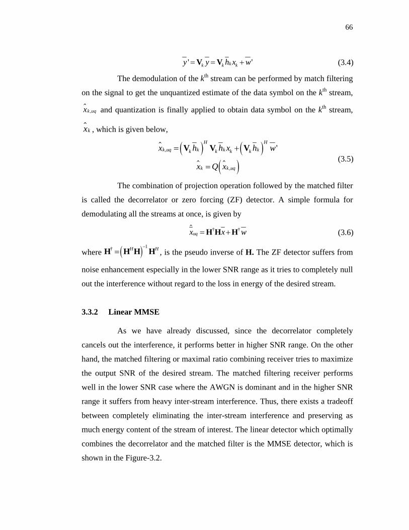
scheme is explained in the flow chart shown in Figure-3.3. The post detection
SNR of the ith data stream is defined as,
{ }2
22
i
iin
E x
Wρ
σ= (3.10)
For the linear detection schemes, the post detection SNR remains the
same for all the streams. However, for the SIC method, the post detection SNR of
the stream increases in each stage and it is lower bounded by their corresponding
post detection SNR obtained without interference cancellation. Thus, the
performance of the SIC scheme is better compared to its corresponding linear
detection scheme. It is assumed that the stream detected at each stage is perfect,
however, the wrong decisions may lead to error propagation. The SIC scheme
Input , yH
( )
( )( )
†
†
r
is the ith row of matrixwith dimension N x1
i i i
i i
i i i
W
W
x Q W y
=
=
H
H
STOP
[ ][ ]
1
i+1
where is the ith column of matrix
is obtained by makingzeroing columns 1,2,...i+1 of H
ii i i
i
y y x+ = − H
H H
H
Figure 3.3: Flow chart of the SIC – Decorrelator
i=1; H1=H
Is i = Nt Yes
No
i=i+1

69
described here follows an arbitrary ordering; for instance, order can be from
stream 1 to Nt.
3.3.4 VBLAST The order in which the streams are detected in the SIC impacts the
performance as it might lead to error propagation. The VBLAST detection scheme
is same as the SIC method except that it follows an order for detection of the
streams at each stage. It is also called as ordered SIC (OSIC). It is proved in
(Wolniansky et al, 1998) that by simply choosing the best iρ at each stage in the
detection process leads to the globally optimum ordering.
The ZF-VBLAST scheme is shown in the flow chart in Figure-3.4, in
which the ZF scheme is used for detection. The MMSE-VBLAST is also an
ordered SIC, in which the MMSE filter is used for detecting the streams and the
ordering is based on the maximum post detection SINR (Hufei zhu, 2004). The
stream which corresponds to the minimum value in the main diagonal of the
matrix, 12
2H n
s
σσ
−⎛ ⎞
+⎜ ⎟⎝ ⎠
H H I is detected first and the effect of that stream is removed
from the received signal and process is iterated to get all streams. The MMSE-
VBLAST has the advantage of both MMSE detection and optimal ordering in the
SIC maximizing the output SINR at each stage and hence it performs better than
the ZF-VBLAST.
3.3.5 Maximum likelihood detection
The objective function of the maximum likelihood detection is given as
2
argminMLx
x y x= −H (3.11)
Where x takes all possible combinations of all symbols from all
streams. The ML method is the optimal and it chooses the transmit symbol vector

70
which minimizes the Euclidean norm between the received signal and all possible
combinations of constellations from multiple transmit antennas. The number of
possible combinations is given by MtN , where M is the constellation size. The
search space increases exponentially with number of antennas and the
constellation size. Though the ML method is the optimal, it is computationally
complex.
Input: H, r
Intialization i=1
( )
†1
2
1 1arg minj
jk
=
=
G H
G
( )ii
k i kW = G
Where ( )i
i kG correspond to
the ki th column of Gi
ii
Tikky W r=
( )i ik ka Q y=
( )1
†1
ii
i
i i k k
i k
r r a+
+
= −
=
H
G H
Where †
ikH is the matrix obtained
by zeroing columns k1,k2..ki of H
{ }( )
1 2
2
1 1, ..
arg minj
i i jj k k k
k + +∉
= G
Is i = Nt
STOP
i=i+1
Figure 3.4: Flow chart of the VBLAST scheme
Yes
No

71
3.4 MIMO-OFDM SYSTEM
The simplified MIMO-OFDM system is shown in Figure-3.5 with
Nt=Nr=2. The incoming symbols are made into a block of size N, where N is the
number of subcarriers and OFDM symbols are constructed and transmitted from
the 2 antennas. The received signal is obtained by passing the transmitted signals
through the multipath channels and AWGN is added at the receivers.
At the receiver, the typical OFDM receiver operations are done in the
two antennas separately to obtain the frequency domain signals. The MIMO
detector is applied at each subcarrier to detect the data transmitted on that
subcarrier. Thus, the MIMO-OFDM system can be viewed as N parallel MIMO
systems with flat fading channel coefficients and the detection has to be
performed on each subcarrier independently (Allert Van Zelst, 2004). The system
forms the basis for the IEEE 802.11n standard proposals.
3.4.1 Mean square error of detection
The mean square error (MSE) between the transmitted data symbols
and the output of the detection algorithm is a good measure for the performance of
MIMO detection algorithms though there is no simple relation with BER or PER.
Since the MSE can be derived for the MIMO detection algorithms, we use the
MSE as performance metric for comparing the various MIMO detection
Figure 3.5: MIMO-OFDM system
h11(n)
w1(n)
w2(n)
h22(n)
h21(n)
h12(n)
s/p
I F F T
p/s
s/p
I F F T
p/s
Multipath channel
CP
CP
CP
s/p
F F T
p/s
s/p
F F T
p/s
MIMO Detector
1 ( )X k
2 ( )Y k
1( )Y k
CP 2 ( )X k
2 ( )X k
1( )X k

72
processes. However, the entire system performance result including the effects of
the encoder etc., can be obtained in terms of the BER and PER and we also show
these simulation results in section 3.4.4. It has been seen in simulations and in
other studies that a reduction in MSE leads to a reduction in the BER. The system
model is shown in Figure-3.5. The MSE is given as follows,
{ }2( ) ( )MSE E x n x n= − (3.12)
The closed form MSE for the decorrelator and the MMSE detector is
derived in Appendix 2 and is given as follows,
{ }H HdecorrMSE E w w= V V (3.13)
( ){ } ( ){ } ( ){ }2 2 2 21 2 32 Remmse t u t u t n t uMSE N N E trace G N E trace G N E trace Gσ σ σ σ ⎡ ⎤= + + − ⎣ ⎦
(3.14)
3.4.2 Low complexity MIMO detection
In a MIMO-OFDM system with N subcarriers typically, we need to
employ N independent MIMO detectors. The system complexity increases with
the increasing number of antennas and particularly in OFDM systems, the
complexity is still more as we might need to employ N parallel MIMO detectors.
In this work, a low complexity solution for a certain type of MIMO
detectors is proposed. The idea is to reduce the number of MIMO detectors
applied for detecting the data in all the subcarriers. As previously discussed, the
IEEE 802.11n channel models have significant amount of correlation across
subcarriers. This frequency correlation among the adjacent subcarrier can be used
to reduce the complexity of the MIMO-OFDM system. Since the channel matrices
for adjacent subcarriers are similar, instead of independently employing MIMO
detectors in all the subcarriers, only the solution for the MIMO detector on
alternate subcarrier positions are found. The solution for the other subcarriers is

73
found by interpolating the solutions obtained for the neighboring subcarriers.
Linear interpolation using weights which are simple to implement can be used.
Let k-1 and k+1 be the subcarrier positions where the direct solution for
MIMO detection is obtained and let k be the subcarrier position in which the
solution is obtained by linear interpolation as given by,
1 1
2k k
k− ++
=V VV (3.15)
Where Vk is the matrix solution for MIMO detection. If the number of complex
multiplications is L for a single MIMO detector, the number of complex
multiplications for applying the MIMO detector independently on each subcarrier
is NxL and with this low complexity method, it becomes (NxL)/2. Thus, there is a
50% reduction in the complexity when compared to the normal MIMO-OFDM
detection methods. Another notable advantage of this method is that there is no
need for the channel estimates on alternate subcarriers. This idea can be used for
ZF, MMSE, MMSE-SIC, ZF-SIC detection method. It cannot be directly applied
to the VBLAST based detection schemes, since the order in which the detection is
performed varies for each subcarrier.
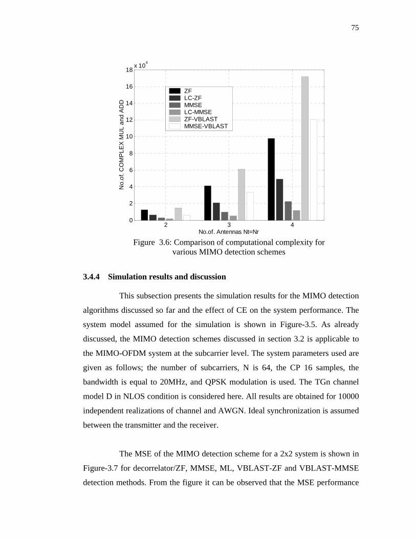
3.4.3 Complexity comparison
The computational effort needed for the MIMO detectors so far
discussed is shown in the Table-3.1. The number of complex multiplications
tabulated here is calculated by considering detection on all the streams and on all
the N subcarrier (Mohammed Alamgir, 2003). The computations required for
various MIMO detection methods is plotted for 2,3,4 transmit and receive
antennas is plotted in Figure-3.6. The value of N assumed is 56.
The decorrelator/ZF solution is the pseudoinverse of the channel
matrix. The MMSE solution requires matrix multiplications and a normal matrix
inverse. The number of complex operations of the MMSE method is less than that

74
of the ZF since the pseudoinverse requires more computations. The non-linear
methods such as ZF/MMSE-VBLAST require more amount of computations as
compared to linear methods as SIC is done and the ordering and filters need to be
calculated for every transmit stream, but as the iteration progresses the number of
complex operations per iteration decreases, because of the reduced (deflated)
channel matrix as there is a decrease in inter-stream interference. The ZF-
VBLAST requires more complexity than the MMSE-VBLAST for the reason
mentioned earlier (Pseudoinverse requires more complexity than normal
inversion). From Figure-3.6 it can be seen that the low complexity detectors LC-
ZF/LC-MMSE have almost half the complexity reduced because of using
interpolated solutions. The complex operations for finding the interpolated
solutions are also included, however, the complexity is drastically reduced, since
the linear interpolation (or) simple averaging doesn’t increase the computations.
The ML detection requires huge amount of complexity which increases
exponentially with more number of transmit and receive antennas since the search
space increases drastically. Thus, ML is generally not preferred for
implementation as compared to other non linear schemes like ZF/MMSE-
VBLAST.
Table 3.1: Complexity comparison
MIMO detector No. of. Complex operations
Decorrelator ( )2 3 25 22r t t tN N N N N+ +
MMSE ( )3 2 25 t t r tN N N N N+ +
LC-ZF ( )2 3 25 222 r t t t t rN N N N N N N+ + +
LC-MMSE ( )3 2 252 t t r t t rN N N N N N N+ + +
ZF-VBLAST ( )2 3 2
15 22
tN
r ti
N N i i N=
⎛ ⎞+ +⎜ ⎟
⎝ ⎠∑
MMSE-VBLAST ( )3 2 2
1
5tN
r ri
N i N i N i=
⎛ ⎞+ +⎜ ⎟
⎝ ⎠∑
75
3.4.4 Simulation results and discussion
This subsection presents the simulation results for the MIMO detection
algorithms discussed so far and the effect of CE on the system performance. The
system model assumed for the simulation is shown in Figure-3.5. As already
discussed, the MIMO detection schemes discussed in section 3.2 is applicable to
the MIMO-OFDM system at the subcarrier level. The system parameters used are
given as follows; the number of subcarriers, N is 64, the CP 16 samples, the
bandwidth is equal to 20MHz, and QPSK modulation is used. The TGn channel
model D in NLOS condition is considered here. All results are obtained for 10000
independent realizations of channel and AWGN. Ideal synchronization is assumed
between the transmitter and the receiver.
The MSE of the MIMO detection scheme for a 2x2 system is shown in
Figure-3.7 for decorrelator/ZF, MMSE, ML, VBLAST-ZF and VBLAST-MMSE
detection methods. From the figure it can be observed that the MSE performance
2 3 40
2
4
6
8
10
12
14
16
18x 104
No.of. Antennas Nt=Nr
No.
of. C
OM
PLE
X M
UL
and
AD
D
ZFLC-ZFMMSELC-MMSEZF-VBLASTMMSE-VBLAST
Figure 3.6: Comparison of computational complexity for various MIMO detection schemes

76
of the ML detector is better than that of all the other schemes. However, the ML
method is computationally complex. The MSE of the ZF detector is directly
proportional to the noise variance and it decreases linearly as the Eb/No increases.
The MMSE detector has a small value MSE in lower Eb/No region compared to
that of the ZF detector since it does not lead to noise enhancement. However, as
Eb/No increases, the MSE tends to approach the MSE of the ZF detector. This is
because in the higher Eb/No region, the performance degradation is mainly due to
inter stream interference. The VBLAST-ZF/MMSE has better MSE performance
compared to the normal ZF/MMSE method because of the OSIC.
A similar plot for 4x4 system is shown in Figure-3.8. It can be
observed from the figure that VBLAST-ZF & VBLAST-MMSE perform well.
This is because the OSIC for 4 streams cancels the interference in successive
stages to get more diversity advantage as discussed in section 3.3.
0 5 10 15 20 25 30 3510-6
10-5
10-4
10-3
10-2
10-1
100
101
102
Eb/N0 in dB
MS
E
ZFMMSEVBLAST-ZFVBLAST-MMSEML
Figure 3.7: MSE performance of various MIMO detection schemes for 2x2 system in channel D, NLOS

77
0 5 10 15 20 25 30 3510-4
10-3
10-2
10-1
100
101
102
Eb/N0 in dB
MS
E
ZFMMSEVBLAST-ZFVBLAST-MMSE
Figure 3.8: MSE performance of various MIMO detection schemes for 4x4 uncoded system in channel D, NLOS
Figure 3.9: MSE performance of various low complexity MIMO detection schemes for 2x2 uncoded system in channel D, NLOS
0 5 10 15 20 25 30 3510-3
10-2
10-1
100
101
102
Eb/N0 in dB
MS
E
LC-ZFLC-MMSEZFMMSE

78
The MSE performance of the low complexity MMSE and decorrelator
is plotted in Figure-3.9. The figure shows that the low complexity
MMSE/decorrelator method performs very close to normal MMSE/decorrelator
method till a point in SNR of 10 dB and has an error floor thereafter and it is
because of using the interpolated solutions on alternate subcarrier positions as
explained in section 3.4.
The BER performance of the MIMO detection schemes is plotted in
Figure-3.10. We can observe that the performance of the MIMO detection
schemes in BER terms is in accordance with their MSE performance i.e., the order
in which the schemes perform is same both in terms of the BER and the MSE. The
LC-ZF/LC-MMSE detector performs close to ZF/MMSE till about 15dB of Eb/N0
and has an error floor of 10-2 in BER, which is quite high. Thus, the LC-ZF/LC-
MMSE are not suitable for uncoded systems, however, it performs well in IEEE
802.11n systems which will be discussed in later sections.
0 5 10 15 20 25 30 3510-6
10-5
10-4
10-3
10-2
10-1
100
Eb/N0 in dB
BE
R
ZFMMSEVBLAST-ZFVBLAST-MMSEMLLC-ZFLC-MMSE
Figure 3.10: BER performance of various MIMO detection schemes for 2x2 uncoded system in channel D, NLOS
79
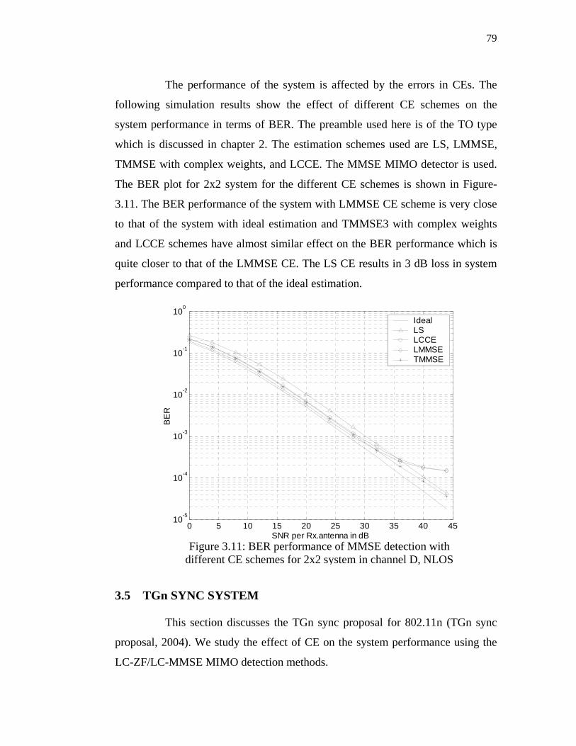
The performance of the system is affected by the errors in CEs. The
following simulation results show the effect of different CE schemes on the
system performance in terms of BER. The preamble used here is of the TO type
which is discussed in chapter 2. The estimation schemes used are LS, LMMSE,
TMMSE with complex weights, and LCCE. The MMSE MIMO detector is used.
The BER plot for 2x2 system for the different CE schemes is shown in Figure-
3.11. The BER performance of the system with LMMSE CE scheme is very close
to that of the system with ideal estimation and TMMSE3 with complex weights
and LCCE schemes have almost similar effect on the BER performance which is
quite closer to that of the LMMSE CE. The LS CE results in 3 dB loss in system
performance compared to that of the ideal estimation.
3.5 TGn SYNC SYSTEM
This section discusses the TGn sync proposal for 802.11n (TGn sync
proposal, 2004). We study the effect of CE on the system performance using the
LC-ZF/LC-MMSE MIMO detection methods.
0 5 10 15 20 25 30 35 40 4510-5
10-4
10-3
10-2
10-1
100
SNR per Rx.antenna in dB
BE
R
IdealLSLCCELMMSETMMSE
Figure 3.11: BER performance of MMSE detection with different CE schemes for 2x2 system in channel D, NLOS
80
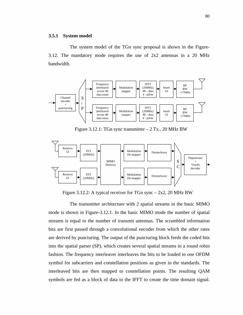
3.5.1 System model
The system model of the TGn sync proposal is shown in the Figure-
3.12. The mandatory mode requires the use of 2x2 antennas in a 20 MHz
bandwidth.
The transmitter architecture with 2 spatial streams in the basic MIMO
mode is shown in Figure-3.12.1. In the basic MIMO mode the number of spatial
streams is equal to the number of transmit antennas. The scrambled information
bits are first passed through a convolutional encoder from which the other rates
are derived by puncturing. The output of the puncturing block feeds the coded bits
into the spatial parser (SP), which creates several spatial streams in a round robin
fashion. The frequency interleaver interleaves the bits to be loaded in one OFDM
symbol for subcarriers and constellation positions as given in the standards. The
interleaved bits are then mapped to constellation points. The resulting QAM
symbols are fed as a block of data to the IFFT to create the time domain signal.
Frequency interleaver across 48 data tones
Frequency interleaver across 48 data tones
Modulation
mapper
Modulation
mapper
S / P
Channel encoder
+ puncturring
IFFT (20MHz) 48 – data 4 - pilots
IFFT (20MHz) 48 – data 4 - pilots
Insert
GI
Insert
GI
RF BW
~17MHz
RF BW
~17MHz
Figure 3.12.1: TGn sync transmitter – 2 Tx., 20 MHz BW
Remove GI
FFT
(20MHz)
FFT
(20MHz)
MIMO Detector
Modulation De-mapper
Deinterleave S C
Depuncture +
Viterbi decoder
Remove GI
Modulation De-mapper
Deinterleave
Figure 3.12.2: A typical receiver for TGn sync – 2x2, 20 MHz BW

81
The pilot tones are also inserted in the frequency domain. The cyclic prefix (CP) is
inserted in the time domain and the windowing of the OFDM symbols is also
performed in the time domain.
A typical receiver for a 2x2 system is shown in the Figure-3.12.2. The
CP is removed from the received signal on the two antennas, which are then
passed through the FFT block to create a frequency domain signal. The received
signal on each subcarrier from the two antennas is passed through the MIMO
detector, which separates out the transmitted streams. Demodulation is done on
each stream, followed by the deinterleaving operation. The spatial combiner (SC)
multiplexes the two streams in a round robin fashion and the bits or the soft values
are passed through the viterbi decoder after suitable depuncturing, which is then
passed through the descrambler to obtain the information bits.
3.5.2 Effect of CE on system performance
In the previous section, we have discussed the effect of CE on the
uncoded MIMO-OFDM systems and the performance of the low complexity
MIMO detection schemes. It is very important to know the amount of
performance degradation due to the CE in terms of BER and PER for IEEE
802.11n. The TGn sync proposal is taken as reference. The CE schemes
considered here are the LS, LMMSE, LCCE and TMMSE. The performance
measure of the system is presented in terms of both BER and PER. The PER is
defined as the ratio between the number of packets received with alteast one bit
error to the total number of packets transmitted. The CEs are obtained from
HTLTF symbols as outlined in the earlier chapter.
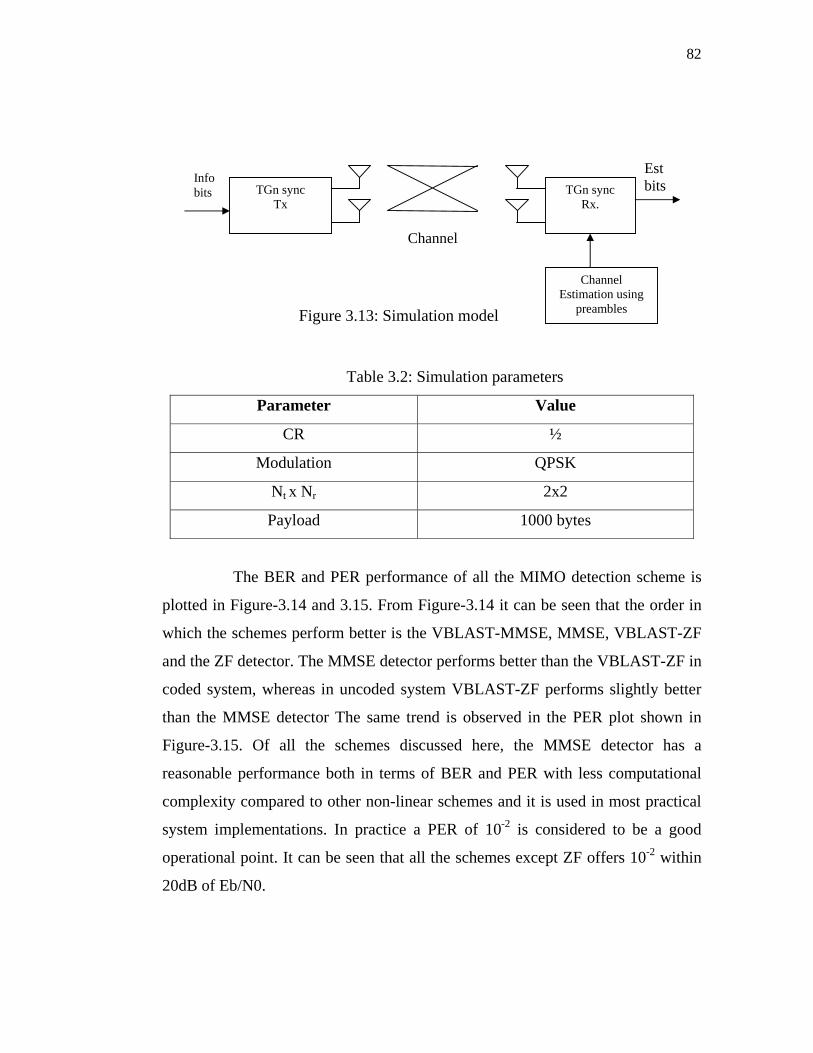
3.5.3 Simulation results and discussion
The simulation model used is given in Figure-3.13. and the simulation
parameters are summarized in Table 3.2. The IEEE 802.11n TGn sync channel
model is used and ideal synchronization is assumed.
82
Table 3.2: Simulation parameters
Parameter Value
CR ½
Modulation QPSK
Nt x Nr 2x2
Payload 1000 bytes
The BER and PER performance of all the MIMO detection scheme is
plotted in Figure-3.14 and 3.15. From Figure-3.14 it can be seen that the order in
which the schemes perform better is the VBLAST-MMSE, MMSE, VBLAST-ZF
and the ZF detector. The MMSE detector performs better than the VBLAST-ZF in
coded system, whereas in uncoded system VBLAST-ZF performs slightly better
than the MMSE detector The same trend is observed in the PER plot shown in
Figure-3.15. Of all the schemes discussed here, the MMSE detector has a
reasonable performance both in terms of BER and PER with less computational
complexity compared to other non-linear schemes and it is used in most practical
system implementations. In practice a PER of 10-2 is considered to be a good
operational point. It can be seen that all the schemes except ZF offers 10-2 within
20dB of Eb/N0.
TGn sync Tx
TGn sync Rx.
Channel Estimation using
preambles
Info bits
Est bits
Figure 3.13: Simulation model
Channel

83
5 10 15 20 25 3010-6
10-5
10-4
10-3
10-2
10-1
100
Eb/N0 in dB
BE
R
ZFMMSEZF-VBLASTMMSE-VBLAST
Figure 3.14: BER performance of various MIMO detection schemes for 2x2 TGn sync system in channel D, NLOS
0 5 10 15 20 25 3010-4
10-3
10-2
10-1
100
Eb/N0 in dB
PE
R
ZFMMSEZF-VBLASTMMSE-VBLAST
Figure 3.15: PER performance of various MIMO detection schemes for 2x2 TGn sync system in channel D, NLOS

84
The BER and PER performance of the LC MMSE/ZF scheme with
BPSK modulation for 2x2 case is shown in the Figure-3.16 and 3.17. From the
BER, PER performance plots it can be observed that the LC MMSE/ZF perform
very close to ZF/MMSE schemes. An error floor less than 10-5 and 10-2 in BER
and PER, respectively, is observed for the LC MMSE/ZF schemes. Thus, the LC
MMSE/ZF does not have performance loss in the useful Eb/N0 region but has a
50% reduction in complexity. The results follow similar trend for 3x3 and 4x4.
The following simulation results show the effect of different CE
schemes on the system performance in terms of BER and PER. We use LS,
LCCE, TMMSE, and LMMSE CE schemes for the TGn sync preamble with
MMSE MIMO detector. The BER and PER performance for 2x2 system for the
different CE schemes in channel D, NLOS are plotted in Figure-3.18 and Figure-
3.19. From Figure-3.18 it can be observed that the LMMSE CE scheme has the
performance very close to that of the ideal CE. The TMMSE with complex
0 5 10 15 20 25 3010-7
10-6
10-5
10-4
10-3
10-2
10-1
100
Eb/N0 in dB
BE
R
ZFMMSELC-ZFLC-MMSE
Figure 3.16: PER performance of LC-MIMO detection schemes for 2x2 TGn sync system in channel D, NLOS

85
weights and the LCCE schemes have almost similar effect on the BER
performance which is quite close to that of the LMMSE CE. The LS CE results in
a 2.75 dB loss in performance compared to that of the ideal CE.
From Figure-3.19 it can be seen that at 10-1 PER the LC CE leads to a
performance loss of about 2.5 dB, the LCCE and RMMSE schemes perform
almost same having a loss less than 1 dB, and the performance of LMMSE
scheme is almost close to that of the ideal CE.
0 5 10 15 20 25 3010-4
10-3
10-2
10-1
100
Eb/N0 in dB
PE
R
ZFMMSELC-ZFLC-MMSE
Figure 3.17: BER performance for various CE schemes with MMSE detection for 2x2 TGn sync system in channel D, NLOS

86
Figure 3.19: PER performance of LC MIMO detection schemes for 2x2 TGn sync system in channel D, NLOS.
5 10 15 20 25 3010-4
10-3
10-2
10-1
100
Eb/N0 in dB
PE
R
LSLCCELMMSETMMSEIdeal
0 5 10 15 20 25 3010-7
10-6
10-5
10-4
10-3
10-2
10-1
100
Eb/N0 in dB
BE
R
LSLCCELMMSETMMSEIdeal
Figure 3.18: PER performance for various CE schemes with MMSE detection for 2x2 TGn sync system in channel D, NLOS

87
The performance gap (Gp) in dB between the ideal CE and the other CE
schemes at 10-5 BER point is plotted in Figure-3.20 for B to F channel models in
NLOS condition. As we move from channel B to F, the Gp increases for the CE
schemes which use the frequency correlation. i.e., the Gp corresponding to channel
B is lesser than that of channel F, since the correlation across the frequency
response of the channel is more for channel B, which could be used to get better
estimates.
3.6 SUMMARY
In this chapter various MIMO detectors are discussed and their
performance in uncoded system in terms of MSE and BER is presented based on
simulation. The effect of CE on the performance of uncoded MIMO system is also
presented. A low complexity solution for MIMO-OFDM detection is proposed
and it reduces the computational complexity by 50%. The performance of the TGn
sync system is presented for various MIMO detection methods in terms of BER
B C D E F0
0.5
1
1.5
2
2.5
3
3.5
Channel models
Per
form
ance
Los
s, G
p
LMMSETMMSELCCELS
Figure 3.20: Gp Loss in performance of 10-5 BER for different CE method on all channel models

88
and PER. It is shown by simulations that the LC MIMO detectors result in very
less performance degradation for practical channel conditions. Thus, the LC
MIMO detectors can be used for IEEE 802.11n proposals as they reduce the
computational complexity load at the receiver.
The effect of various CE schemes on the performance of IEEE 802.11n
TGn sync proposal is presented in terms of BER and PER. The results indicate
that the LS scheme results in about 3 dB loss in performance at 10-5 BER point,
while the low complexity CE schemes such as LCCE, TMMSE have less
performance degradation. Thus, the TMMSE and LCCE CE schemes can be used
for IEEE 802.11n proposals leading to fewer computations and less performance
degradation.
Top Related