


Languages
Pages
Legal


Media Revenue Management with Audience Uncertainty
Victor F. Araman • Ioana Popescu1
Information, Operations and Management Science Stern School of Business, New YorkUniversity, New York, NY 10012, USA
Decision Science Area, INSEAD, Fontainebleau, 77300, France
[email protected] • [email protected]
An important challenge faced by media broadcasting companies is how to allocate limitedadvertising space between upfront contracts and the spot market (referred to in advertisingas the scatter market), in order to maximize profits and meet contractual commitments.We develop stylized optimization models of airtime capacity planning and allocation acrossmultiple clients under audience uncertainty. In a short term profit maximizing setting, ourresults suggest that broadcasting companies should prioritize upfront clients according tomarginal revenue per audience unit, also known as CPM (cost per thousand viewers). Forcapacity planning purposes, accepted upfront market contracts can be aggregated acrossclients. The upfront market capacity should then be allocated to clients in proportion totheir audience requirement. Closed form solutions are obtained in a static setting. Theseresults remain valid in a dynamic setting, when considering the opportunity to increaseallocation by airing make-goods during the broadcasting season. Our structural resultscharacterize the impact of contract parameters, time and audience uncertainty on profitsand capacity decisions. The results hold under general audience and spot market profitmodels. Our numerical results, based on real data, suggest that the benefits from modelingaudience uncertainty in the media revenue management context can be significant.
1. Introduction
Optimally managing and valuing limited advertising space is one of the key problems faced by
media companies today (Alvarado 2007, Zhang 2006). This paper provides formal models
and solutions for the problem of managing broadcast advertising capacity. We begin by
describing how advertising is sold, in order to illustrate the complexities of this problem,
and motivate the focus of our work. This introduction further highlights our contribution
and related literature, and introduces industry-specific terminology.
1This author’s research was funded by the Booz & Co. Chair in Revenue Management at INSEAD.
1

1.1 The Media Broadcasting Advertising Market
In the 1930s, the sponsorship of radio serials by makers of household-cleaning products
led to the soap opera. Listeners were enthralled by episodic, melodramatic storylines, and
advertisers were guaranteed a big audience. According to TNS media intelligence, 2006
U.S. advertising spending exceeded USD 150 billion. Of this, television accounts for 44%,
with advertisers ready to pay up to half a million dollars for a 30 second commercial in
a popular show such as Friends, and new-show campaigns reaching up to USD 10 million
(source adage.com). According to the A.C. Nielsen Co., the average American watches more
than 4 hours of TV each day, 30% of which is advertising (source: nielsenmedia.com).
Media broadcasting companies such as TV channels, cable networks or radio stations
collect most of their revenues from selling impressions (“eye-balls”), through advertising
space (30 second commercial slots) during various programs. Typically, in north America
and several European countries, the bulk of advertising space (about 60-80%) is sold during
an upfront market, following the announcement of program schedules and prices for the year.
In the US, the upfront market occurs during less than a couple of weeks in May, much before
the broadcasting season starts in mid-September. During this period, a few major advertisers
(MA) buy long term contracts (called media plans, or campaigns) from the broadcasting
company (BC) at relatively low margins. In reality, sales are either direct or managed by
intermediary buying and selling houses which represent their respective clients’ interests. Our
results and analysis are relevant to the party in charge of the capacity planning and revenue
management function, for simplicity referred to as broadcasting company (BC). Upfront
contracts stipulate a budget to be spent throughout the year, and a cost per thousand viewers
(CPM ), the ratio of the two providing a target level of audience (or ratings) to be reached by
the campaign. The remaining advertising space is sold throughout the broadcasting season
on a spot market, called scatter market in the industry, on a price-per-slot basis, usually at
a higher margin and with no audience guarantee.
This paper investigates the problem of optimally managing media advertising capacity.
This problem resembles in many ways the standard capacity control paradigm in revenue
management (see Talluri and van Ryzin 2004 for a comprehensive treatment and Elmaghraby
and Keskinocak 2003 for a review). In this problem, a service provider allocates limited
capacity (e.g. seats on a flight or rooms in a hotel) between customer classes with different
valuations and arrival patterns (e.g. business and leisure customers). Similarly, in the media
2
revenue management problem, the broadcasting company allocates limited advertising space,
called airtime or media capacity, between two customer classes: upfront (market) clients, who
buy early during the upfront market at high discounts, and scatter (market) clients, who
buy later on the spot (or scatter) market at higher prices. Advertising capacity is fixed,
by physical time limitation and regulations.2 Revenue management is particularly relevant
when capacity is tight, which is the case for example with prime-time advertising.
Several specificities differentiate the problem of managing media capacity from the stan-
dard revenue management setup. First, unlike traditional revenue management, in the media
problem the value of advertising capacity is uncertain at the time when capacity allocation
decisions are made. This is because upfront contract pricing is state contingent: the amount
paid by an upfront client for a 30 second advertisement is determined by the audience
reached, multiplied by the negotiated rate per viewer (CPM). Audience (i.e. the number
of viewers, or impressions) is unknown ex-ante, when capacity allocation is made, but pro-
vided ex-post by media rating agencies. Therefore, in managing advertising capacity, the
broadcasting company (BC) bears the risk of audience uncertainty in the upfront market.
The value of an advertising slot depends both on the uncertain audience level, and on the
opportunity cost of selling it later on the scatter market. Our goal is to develop a rev-
enue management framework for valuing and managing limited advertising capacity under
audience uncertainty.
Other important differences from traditional revenue management stem from the media
B2B setting: transactions are contract based, upfront clients hold a strong bargaining power
and retention of key accounts is an important strategic issue.3 Strategic decisions, such as
rate card pricing and contracting, while highly relevant, are best addressed in a competitive,
long term profitability setting. This paper focuses on the short term profit maximization
problem of the firm in managing advertising capacity between upfront and scatter markets,
with given contracts and prices, during one broadcasting season. We refer to this as the
media revenue management, or capacity planning problem.
The media revenue management problem is a highly complex multi-level problem (Zhang
2006). Industry practice, organizational and technical considerations, all argue for a hier-
2In Europe for example, EU directives restrict advertising to 15% of total airtime, with at most 12advertising minutes per hour, and not more than one break per movie. American regulations are less strict(about 30% of airtime).
3This partly explains the large volume sold at low margins upfront; other arguments include stock marketsignaling, account executive incentives, BC’s risk aversion.
3

archical planning approach, separating strategic, operational and tactical layers of decision
making. First, during the upfront market, the BC negotiates contract allocation and es-
timates overall capacity requirements for the upfront clients; this is known in practice as
the strategic or upfront planning phase. Subsequently, account executives allocate an initial
portion of advertising capacity to the client (known as a media plan or sales plan), with
the provision that additional capacity, so-called make-goods (or audience deficiency units,
ADU), will be allocated during the scatter market if the plan under-performs. Sequential
make-goods allocation decisions are made periodically during the rest of the year; this is
called operational planning. At the tactical planning level, individual commercials are sched-
uled in breaks, accounting for product conflict and other scheduling constraints. A detailed
description of this process is provided in Section 2.2.
Current practice in the industry is to make such decisions qualitatively (see e.g. Bol-
lapragada and Mallik 2007, Zhang 2006). With the notable exception of a few companies
(e.g. NBC), who use models for scheduling commercials in breaks, to our knowledge, no
mathematical model is currently being used for capacity planning or make-goods allocation.
Previously published work on media revenue management has focused on providing algo-
rithms for scheduling commercials in breaks and generating sales plans, based on complex,
deterministic combinatorial models (Bollapragada et al. 2002, Bollapragada and Garbiras
2004, Zhang 2006, Kimms and Muller-Bungart 2007; the first two refer to models imple-
mented at NBC, see Section 1.3 for details).
In contrast, our goal is to provide insights from incorporating the effects of audience
uncertainty in upfront and operational planning decisions. Specifically, we are interested in
how the amount of inventory allocated to the upfront market should be adjusted to hedge
for variability in ratings, both before and during the broadcasting season (make-goods). Our
structural results characterize the sensitivity of capacity decisions to key contract parame-
ters, audience and time. In order to tractably capture the effect of uncertainty on profits
and decisions, we propose stylized, stochastic models which capture aspects of the media
revenue management problem where audience variability is most relevant, and likely to af-
fect decisions. Specifically, we focus on high level, aggregate capacity planning decisions.
For the sake of focus and tractability, we do not address tactical, combinatorial decisions
such as matching clients to programs and scheduling of commercials in breaks, previously
addressed in the literature (in a deterministic setting). We also do not address strategic level
decisions such as rate card pricing and upfront negotiation, best analyzed in a competitive,
4

long-term profitability setting. Our insights can ultimately be incorporated into other layers
of decision making, such as scheduling, which ignore variability in ratings.
1.2 Structure and Results
The paper is structured as follows. The next section reviews related work and positions our
contribution in the media broadcasting, revenue management and random yield literature
streams. Section 2 provides further background about the media problem and business
model, allowing us to set up the terminology, modeling ingredients and assumptions. We
discuss models of audience uncertainty, as well as upfront and scatter market revenue models.
Section 3 derives insights from a simple static, aggregate model for upfront capacity
planning under audience uncertainty. This model is similar to classical random yield and
newsvendor models. We investigate the impact of audience uncertainty on the model, profits
and decisions. In particular, we find that shows with (stochastically) larger, or less variable,
audiences do not necessarily command lower capacity allocations. We further provide static
upfront planning recommendations across multiple periods (air-dates or quarters) or shows.
The results described so far focus on aggregate models of capacity allocation for upfront
vs. scatter markets. Section 4 analyzes capacity allocation decisions across multiple cus-
tomers. Our main result is that upfront clients can be aggregated for capacity planning and
make-goods allocation. Individual client allocations are obtained by solving a single aggre-
gate model for the entire upfront market, and allocating the resulting capacity in proportion
to clients’ performance targets. These results provide the BC with insights for upfront con-
tract negotiation and capacity planning tasks. For modeling purposes, these results allow us
to simplify the analysis by focusing on aggregate planning models.
Section 5 focuses on how capacity decisions are operationalized. We propose dynamic
models for “make-goods” vs. scatter market allocation during the broadcasting season, when
audience, modeled as a stochastic process, is revealed periodically. Our structural results
show that initial capacity commitment to the upfront market should be minimal (known
in the industry as “gapping”), and the optimal make-goods allocation policy is a monotone
threshold type policy.
Section 6 provides numerical insights based on real data, obtained from a major broad-
casting network. In a static (aggregate) setting, we find that ignoring audience uncertainty in
upfront decisions leads to significant profit loss and allocation error (exceeding 30%), in the
context of the data at hand. We propose several simple and intuitive heuristics for dynamic
5

make-goods allocation. We find that policies which take audience uncertainty into account
(e.g. resolving myopic and static heuristics) provide very good approximations for the op-
timal value function, and significantly outperform policies based on deterministic audience
models.
The last section concludes, outlining opportunities for further research.
1.3 Literature and Positioning
The marketing literature has extensively investigated the impact of TV advertising on the
consumer and sales (staring with Metheringham 1964, see also Kanetkar et al. 1992 and
Lodish et al. 1995), but largely ignored the issue of airtime capacity planning. Despite
its richness and complexity, the media revenue management problem has received limited
attention in the operations literature. Chapter 10.5 of Talluri and van Ryzin (2004) provides
a brief account of the media revenue management problem (this book is the most complete
reference on revenue management to date).
Previous papers on broadcast inventory and revenue management focus on scheduling
problems, using deterministic, combinatorial models. Referring to algorithms successfully
implemented at NBC, Bollapragada et al. (2002) and Bollapragada and Garbiras (2004)
present sales plan generation models for single, respectively multiple clients. These models
are deterministic version of those in Section 3.3, which in addition account for scheduling
constraints (e.g. show mix and product conflict), but ignore spot market opportunity costs
and audience uncertainty. Zhang (2006) uses a two-step hierarchical approach to first select
advertisers and match them with shows (winner determination), and then schedule their
commercials to individual slots within a specific show (pod assignment). An integrated
approach is proposed by Kimms and Muller-Bungart (2007). The first two papers use lin-
ear penalties for violated constraints (e.g. client targets), whereas the latter two force all
constraints to be met.
In contrast with previous work which focused on scheduling media plans using determin-
istic models, this paper uses a stochastic model to capture the big picture that is driven
by uncertainty in ratings. Parallel work by Bollapragada and Mallik (2007) shows how a
risk averse BC should allocate rating points between aggregate upfront and scatter markets,
when audience and scatter market revenues are uncertain and independent. Target revenue
and value (revenue) at risk objectives are optimized in a static one period model that ag-
gregates demand from each market, similar to our aggregate model in Section 3. They also
6

provide comparative statics with respect to audience parameters. In their model, the sole
decision variable is the total number of rating points sold in the upfront market. There is no
specification of how this translates into actual capacity allocation, and how this allocation is
“operationalized” across clients and over time. Our work complements theirs by answering
these questions in a risk neutral context.
Besides media, there are several industries where capacity is sold partly in a forward
(advance purchase) market and partly on a spot market, such as electricity markets, cargo
shipping, manufacturing etc. A growing body of literature, reviewed by Kleindorfer and
Wu (2003), investigates inventory management in such settings. Wu and Kleindorfer (2005)
develop a two-stage framework that integrates spot market transactions with supply chain
contracting. In a multi-period model, Araman and Ozer (2005) study optimal inventory
allocation between a long term sales channel and a spot market. Work in this area focuses
mainly on production models under demand uncertainty and supply contracts.
One feature that distinguished the media problem from the above literature, and much of
the operations literature, is the uncertain value of supply: audience is contracted for, but only
realized after airtime capacity allocation is made. This aspect makes our problem similar to
production planning models under random yield, for which Yano and Lee (1995) provide an
excellent review. Specifically, our static models are equivalent to the random yield model
proposed by Shih (1980), with no holding cost, non-linear salvage value and deterministic
demand. Our multiplicative performance model corresponds to a stochastically proportional
(SP) yield model (see Yano and Lee, 1995, and references therein). Because of the lack
of holding costs, our models can be viewed as a special case of those used in the random
yield literature. At the same time, our models are more general, in that they allow general
audience (yield) distributions, and performance measures.
The dynamic make-goods allocation model in Section 5 falls in the class of multiple
lotsizing in production to order (MLPO) with random yield problems, surveyed by Grosfeld-
Nir and Gerchak (2004) (see also Yano and Lee 1995, page 321). Such models aim to satisfy
a fixed initial demand target through a pre-specified number of production runs to minimize
inventory (holding and penalty) costs. In each production run, a random output is produced,
that is a function of the lot size decision. In our case, the input decision is the number of ads
to air for a client, and output is the audience (or ratings) for these ads. Finite horizon models
that come closest to our work are studied by Sepheri et al. (1986), under a binomial yield
distribution and Guu and Zhang (2003), for interrupted geometric (IG) yield distributions
7

(as opposed to SP). Both papers use a distribution specific approach, but allow for non-zero
holding costs. Due mainly to the absence of holding costs, we are able to obtain several
structural results for the media problem, which do not always hold for random yield/MLPO
problems. These include monotonicity of run size (capacity allocation x) with respect to
demand (target audience N) and number of runs (horizon length). Moreover, our results
hold for general yield models (performance Ψ).
In summary, despite modeling similarities, our results (except for Proposition 1) are
different, and cannot be implied from the random yield literature. While our results are
specific to the media problem, they can be viewed as a contribution to random yield problems
without holding costs.
2. Audience and Revenue Models and Assumptions.
This section provides further background for the media revenue management problem and
business model. We describe the main ingredients of our models, including upfront and
scatter market contracting terms, as well as audience and performance measures.
Our models and results focus on prime time inventory allocation, where RM is most
relevant, because capacity is constrained and advertisers’ willingness to pay is high, due to
large viewing audiences.4 Throughout the paper, an ad, or slot, corresponds to one unit of
airtime capacity, e.g. a 30 second slot during a commercial break in a (prime-time) program.
For example, an hour long show in the US typically contains five to seven one to two minutes
long commercial breaks (a.k.a. pods), each containing a set number of advertising slots.
2.1 Audience and Performance Models
An important contribution of this paper is to specifically consider the impact of audience
uncertainty in the media planning task. Hence, an important prerequisite for our work is
to understand ex-post audience metrics and motivate ex-ante forecast models of audience
variability and campaign performance.
Audience is the gross sum of all media exposures (the number of impressions, or “eyeballs”
watching a given show), regardless of duplication. This is unknown ex-ante, but provided
ex-post by media rating agencies, such as Nielsen Media Research in the US, or Mediametrie
4TV prime time includes all regularly scheduled programs 8:00pm-11:00pm (EST) Monday to Saturdayand 7:00pm-11:00pm on Sunday. Average prime-time price is USD 200, 000 per 30 second slot (see Zhang2006).
8

in France. Another popular metric is GRP (gross rating point), also known as rating,
the percentage of the target audience reached by an advertisement.5 Because the ratio of
audience to GRP is a constant (the number of TV viewers/households), the two terms are
used interchangeably with no loss of generality.
To obtain ratings forecasts, the audience (or equivalently GRP) that will be viewing an
ad is modeled ex-ante as a positive random variable ξ with mean µ, standard deviation
σ, distribution F and density f . Its realization, as well as relevant metrics, are provided
ex-post by media rating agencies. For example, a subjective probability q that each of M
potential viewers watches a given show suggests a binomial model ξ ∼ Bin(M, q), which for
large market sizes M could be approximated by a normal distribution. All our results are
distribution independent.
The performance of a media plan is the sum of the ratings obtained for each ad aired.
In order to assess the ex-ante performance of a media plan under audience uncertainty,
our models make several simplifying assumptions. Specifically, (1) we focus on modeling
prior uncertainty in ratings ξ (within the relevant allocation period), and (2) assume that
inventory is homogeneous, i.e. different ads capture similar audiences. These assumptions,
discussed below, allows us to model the ex-ante performance from allocating x homogeneous
slots with prior audience uncertainty ξ, as Ψ(x, ξ) = xξ. This multiplicative performance
model essentially assumes that the GRP for each ad is the same, but unknown ex-ante, i.e.
an a priori unknown fraction of the population views a constant fraction of the ads. In
the upfront market, ξ captures the high level prior uncertainty, before the season starts,
regarding the channel’s share of audience. During the broadcasting season, ξ captures lower
level prior uncertainty about popularity during a particular month or quarter.
An important quantity used in practice and throughout the paper is the GRP allocation,
defined by w = N/x, where N is a client’s performance target. Under the multiplicative
model, this corresponds to the average ratings (i.e. realized audience ξ) for which the per-
formance target N is exactly met by allocating x units of advertising space.
The multiplicative performance model corresponds to the stochastically proportional
yield model used in random yield problems (Yano and Lee, 1995) where the fraction of
output (good) units is random and independent of the input units. Its main advantage is
5For example, during the week of November 20, 2006, the ABC show “Desperate Housewives” toppedthe US household ratings at 13.5, meaning that 13.5% of the estimated 110.2M TV households in the USwatched the show that week.
9

that it is simple to work with and fairly general. Our sensitivity results for upfront and
dynamic make-goods allocation extend for more general performance models of the form
Ψ(x, ξ), with Ψ an increasing function of both arguments and concave in x. Concavity is
justified by “repetition wearout”, i.e. the diminishing marginal benefit of repeatedly reaching
the same individuals.
The multiplicative performance model, defined above, is most appropriate when inventory
is homogeneous. In reality, this is not the case: media plans spread over multiple shows, and
audience varies by show and air-date, and across demographic segments. The homogeneous
inventory assumption is reasonably realistic, if we focus on capacity allocation for a specific
show, or day-part (prime-time in our case), in a specific demographic. In practice, clients
have specific prime-time targets, show preferences and demographic requirements, and the
BC matches clients to shows that provide the best value in their desired demographics (a.k.a.
winner determination, see Zhang 2006). Assuming that clients and prime-time programs
are pre-partitioned by demographics, the inventory allocation problem becomes separable,
favoring the homogeneous inventory assumption. This is appropriate, for example, in French
TV markets, where the level of demographic segmentation is low.
In reality, there is more variability in audience than prior popularity effects captured
by our multiplicative performance model. Prime-time audience varies from week to week,
even for the same show. Section 3.3 provides an aggregation method that deals with such
variability. The next example suggests how the multiplicative model can be viewed as a first
order approximation of a more complex model, which captures audience variability across
individual ads.
Example 1. The total number of (possibly duplicated) impressions from airing x ads
with audiences ξ1, . . . , ξx is the convolution ξ(x) = ξ1 + · · · + ξx. If the number of ads x
is large and audiences are i.i.d., the central limit theorem insures that ξ(x) ∼ N(xµ, xσ2).
However, audiences for a given show are usually highly correlated, especially within a narrow
time-frame. Assuming they are exchangeable (i.e. their joint distribution is not affected by
permutations of the individual random variables), jointly normally distributed with mean µ,
variance σ2 and correlation ρ, we obtain that ξ(x) ∼ N(xµ, (1−ρ+xρ)xσ2). Hence, denoting
Z ∼ N(0, 1), we have:
Ψ(x, ξ) = ξ(x) = xµ + σ√
x(1− ρ + xρ) Z = x
(µ + (ξ − µ)
√1− ρ
x+ ρ
),
10

which is increasing concave in x. Because x is large and ρ is high, ignoring second order
terms, we obtain Ψ(x, ξ) ' x(µ +
√ρ(ξ − µ)
)= xζ, where ζ =
√ρξ + (1−√ρ)µ. Hence we
can approximate Ψ by a multiplicative model corresponding to a modified audience ζ, with
additional point-mass at the mean. In particular, if audiences are perfectly correlated ρ = 1,
we obtain ξ(x) ∼ N(xµ, x2σ2), which has the same distribution as the multiplicative model
xξ. �
2.2 Revenue and Business Model, Terms and Decisions
This paper focuses on (short term) revenue maximization from selling advertising space to
upfront and scatter markets. We next describe the business and revenue models governing
these markets. For details regarding business processes see Bollapragada et al. (2002).
Upfront Market. Following the announcement of program schedules and list prices
in May, clients contact the BC with upfront market requests to purchase advertising space
in bulk, for the entire season. A typical request consists of a budget B for the entire
year, and a negotiated CPM (cost per thousand viewers) C.6 This translates into a target
performance N = B/C, measured by the total audience of the campaign, in the client’s
desired demographic (e.g. men between 18 and 49 years old, or adults 25 to 54). Audience
is unknown ex-ante, but provided ex-post by media rating agencies. Additionally, the MA
may specify performance targets for specific periods (quarterly or weekly weighings) and
programs (e.g. preferred shows, prime time targets). In response to the sales request, the
BC provides a sales plan or proposal, consisting of a list of commercials to be aired, by show
and airdate; the specific break location is decided later, close to broadcasting time. For
examples of plan requests and proposals, see Figures 3 and 4 in Bollapragada et al. (2002).
Because upfront contracts offer performance guarantees, the BC bears the risk of audience
uncertainty. If the plan exceeds contracted performance, i.e. ratings exceed GRP allocation,
the BC receives no additional payment. On the other hand, the BC is penalized (e.g.
by providing make-goods) if at the end of a season a plan has under-performed (e.g. if
large ratings were committed upfront for a show that turns out to be a miss). Our models
account for unmet performance targets via a constant unit penalty b, which amounts to a
total penalty cost of: b · (N −NT )+, where NT is the performance of the plan, i.e. the total
6For example, in 2005, US TV advertising budget for P&G, the largest US advertiser, was $2.5 Billion,whereas Toyota’s was half a billion. American prime time CPM averaged between $20-$35 for TV, and$8-$10 for cable.
11
number of impressions delivered by the end of the season. Penalties are not contractual, they
are a mechanism to model and control under-performance. This approach is consistent with
the previous literature (Bollapragada et al. 2002, Bollapragada and Mallik 2007). Under-
performance penalties are a natural interpretation of strategic service constraints, whereby
the BC commits to satisfy (aka ’steward’) client requests within a given probability, or
expected fraction. In practice, this is uniformly high, around 95%.
In summary, the direct expected profit from an upfront market client is the result of the
client’s budget B minus the expected penalty cost of failing to meet the audience target
b · (N − NT )+, realized at the end of the season. In particular, under the multiplicative
performance model discussed in Section 2.1, if x (homogeneous) slots with audience ξ are
allocated to the client, the expected penalty cost is bE[N − xξ]+. The model so far does not
account for the opportunity cost of allocating capacity to the scatter market, discussed next.
Scatter Market. As opposed to upfront contracts which are audience/CPM based,
scatter market pricing is per advertising slot, with no audience guarantee. Broadcasting
companies typically have to commit list prices for the scatter market in advance. On top
of these baseline prices, the BC applies discounts based on buyer characteristics (bundle,
volume, loyalty) and capacity status. If advertising capacity is Q, and x ≤ Q slots are
allocated to the upfront market, the expected scatter market profit from the remaining
Q− x slots is denoted π(x). This is a general model, which can implicitly allow for scatter
market price and demand to be audience dependent, and price to decline with available
capacity. To see this, let for example π(x) = Eξ[Π(Q− x, ξ)], where Π(y, ξ) = p(y, ξ)S(y, ξ)
is the scatter market profit from y available advertising slots with audience ξ, and S is the
number of ad slots sold at price p(y, ξ), given capacity level y.
All our structural results hold under a general scatter profit model π(x) that is decreasing
and concave in x, accounting for diminishing marginal returns to the scatter market. For
simplicity of exposition, the next section (only) focuses on linear models π(x) = p(Q − x),
corresponding to a constant scatter market price p per advertising slot. This allows for closed
form solutions and clearer insights with no loss of generality.
For convenience, Table 1 summarizes the main notation used in the paper.
Decision Making Layers. The following hierarchical decision making approach reflects
industry practice, and motivates our approach in this paper. At the strategic planning phase,
the BC must decide which client contracts to accept upfront. For this purpose, the firm needs
to assess how much capacity is required to satisfy upfront market clients. This capacity is
12
not committed to the client upfront; it serves only for (strategic) capacity planning purposes
at the upfront stage. At the operational level, the decisions of how much initial capacity to
commit to the upfront clients/market are made, with the specific provision of subsequent
make-goods allocation during the scatter market. During the broadcast season, the BC
periodically decides how many additional make-goods to allocate to upfront clients (vs. the
scatter market), given the current performance of a campaign.
We begin by investigating aggregate capacity planning and allocation decisions under
audience uncertainty, for the upfront market as a whole, and then extend the results to
handle multiple upfront clients.
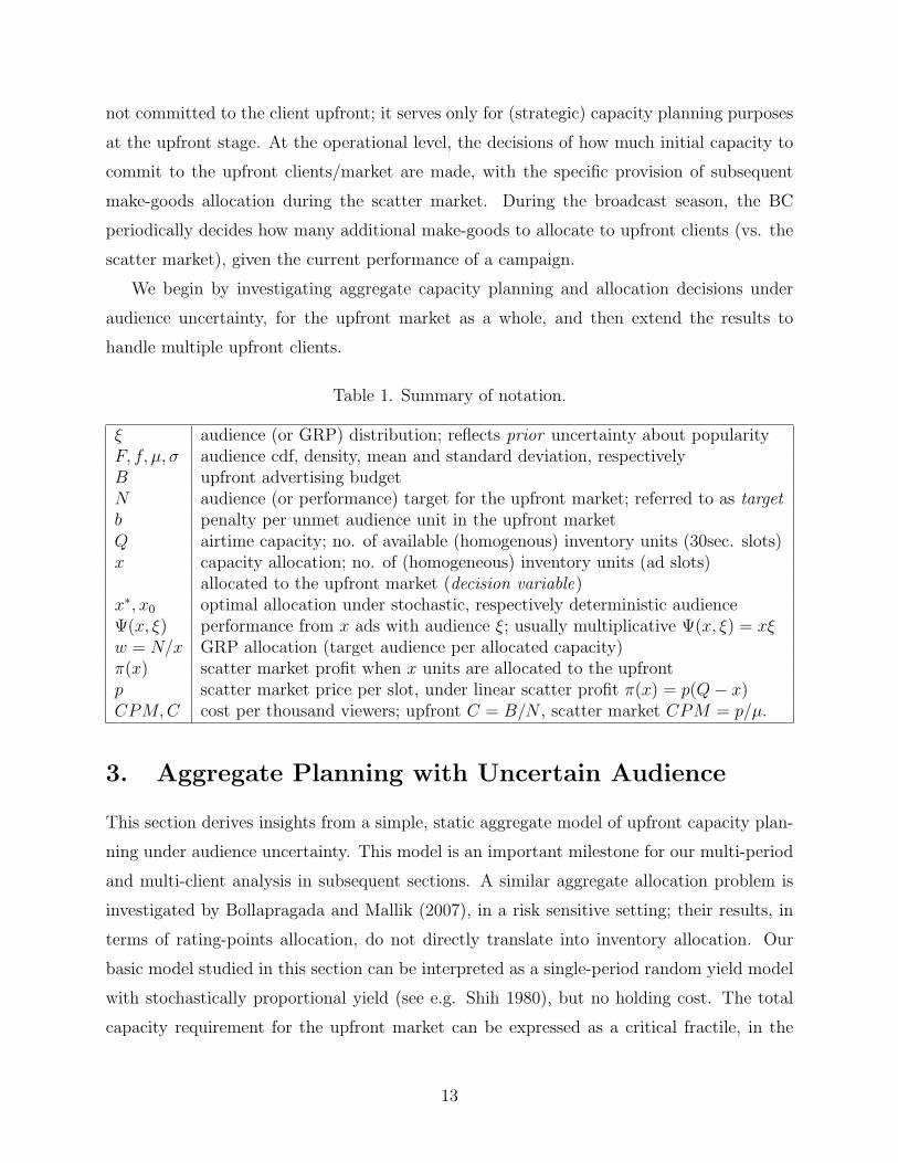
Table 1. Summary of notation.
ξ audience (or GRP) distribution; reflects prior uncertainty about popularityF, f, µ, σ audience cdf, density, mean and standard deviation, respectivelyB upfront advertising budgetN audience (or performance) target for the upfront market; referred to as targetb penalty per unmet audience unit in the upfront marketQ airtime capacity; no. of available (homogenous) inventory units (30sec. slots)x capacity allocation; no. of (homogeneous) inventory units (ad slots)
allocated to the upfront market (decision variable)x∗, x0 optimal allocation under stochastic, respectively deterministic audienceΨ(x, ξ) performance from x ads with audience ξ; usually multiplicative Ψ(x, ξ) = xξw = N/x GRP allocation (target audience per allocated capacity)π(x) scatter market profit when x units are allocated to the upfrontp scatter market price per slot, under linear scatter profit π(x) = p(Q− x)CPM,C cost per thousand viewers; upfront C = B/N , scatter market CPM = p/µ.
3. Aggregate Planning with Uncertain Audience
This section derives insights from a simple, static aggregate model of upfront capacity plan-
ning under audience uncertainty. This model is an important milestone for our multi-period
and multi-client analysis in subsequent sections. A similar aggregate allocation problem is
investigated by Bollapragada and Mallik (2007), in a risk sensitive setting; their results, in
terms of rating-points allocation, do not directly translate into inventory allocation. Our
basic model studied in this section can be interpreted as a single-period random yield model
with stochastically proportional yield (see e.g. Shih 1980), but no holding cost. The total
capacity requirement for the upfront market can be expressed as a critical fractile, in the
13

spirit of the classical newsvendor problem. This allows us to further analyze the impact of
audience uncertainty on profits and managerial decisions.
3.1 Aggregate Upfront Planning.
An important question faced by media revenue managers is how much capacity should be
allocated to upfront vs. scatter markets. In particular, once a given budget and audience
target have been contracted upfront, what is the corresponding capacity requirement for the
entire broadcasting season (see e.g. Alvarado 2007)? Central to our derivations is a simple
aggregate upfront planning model, which answers the latter question by collapsing all upfront
client targets into one cumulative audience target N . Based on the model and assumptions
set up in Section 2, the total expected cost of allocating x homogeneous capacity units with
uncertain audience ξ to the upfront market can be expressed as:
c∗(N) = min0≤x≤Q
px + bE[N − xξ]+. (1)
The main trade-off captured by this model is between the opportunity cost p of allocating
a slot to the spot market and the penalty cost of not meeting the performance target N of
the upfront market. In this section only, we focus on constant scatter market prices p, for
cleaner insights; all our results extend for non-linear scatter market profits.
Recall that F is the cdf of audience uncertainty ξ (as described in Section 2.1), and
denote its left tail expectation by:
G(u) = E[ξI(ξ ≤ u)], (2)
where I(·) denotes the indicator function. This allows to write the cost objective in (1), i.e.
the cost of allocating x units of capacity to the upfront, as:
c(N, x) = px + bE[N − xξ]+ = px + b[NF (N/x)− xG(N/x)
]. (3)
The next result follows directly from the first order conditions, by convexity of the cost
function and monotonicity of G. Its proof is omitted for conciseness. Throughout the paper,
increasing/decreasing refer to weak monotonicity.
Proposition 1 The optimal solution to Problem (1) is x∗ = min(Q, x), where the uncon-
strained optimum x satisfies:
G(N/x) = p/b. (4)
14

Furthermore, x∗ is piecewise linear and increasing in the target performance N , increasing
in the penalty b and decreasing in the spot price p, all else equal. The optimal cost c∗(N)
equals bNF (G−1(p/b)), if p/b ≥ G(N/Q) and c(N, Q) otherwise.
Incidentally, Proposition 1 suggests that the penalty level b effectively corresponds to
offering a type 1 service level 1− ε = 1− P(x∗ξ ≤ N), which satisfies G−1(p/b) = F−1(ε).
Relation with Random Yield and Inventory Models. In the media revenue man-
agement problem, demand, measured in audience units, is deterministic (N), whereas the
value of allocated supply is uncertain (xξ). This makes our problem akin to production
problems with random yield. Problem (1) is a special case of a single-period random yield
model due to Shih (1980), with stochastically proportional yield and no holding cost (see
also Yano and Lee 1995, page 318). In this problem, x units are produced at a unit cost p.
Of these, an uncertain fraction ξ (the yield rate) satisfies quality standards and can be used
to satisfy demand. Demand is “rigid” and equal to N, and unit shortage cost is b.
Alternatively, Problem (1) can be recast as a single-period newsvendor problem, with
lost sales and no holding cost (Porteus 2002). This is achieved by translating all model
ingredients, in particular demand, in terms of inventory units (i.e. 30 second advertising
slots). The transformation is particularly appealing because the BC’s operational decision
is necessarily in terms of advertising space.
Remark 1 Problem (1) is equivalent to an inventory model with cost = p, price = bµ,
demand θ with cdf P(θ ≤ x) = 1 − G(N/x)/µ, and objective c(N, x) = px + bµEθ[θ − x]+.
The corresponding critical fractile solution, equivalent to (4), is
P(θ ≥ x) =p
µb. (5)
Proof: First note that the cdf of θ is well defined because G(u) is increasing and bounded
in [0, µ]. We can write θ = N/ζ, where ζ is a random variable with cdf P(ζ ≤ u) = G(u)/µ
(also well defined for the same reasons). Indeed, P(θ ≤ x) = 1−G(N/x)/µ = P(ζ ≥ N/x).
The objective in Problem (1) can be recast as follows:
c(N, x) = px + bµE[ξ/µ(N/ξ − x)+] = px + bµEζ [N/ζ − x]+ = px + bµEθ[θ − x]+.
The second equality is based on a change of measure transformation from ξ to ζ. By defini-
tion, ζ has density h(u) = u/µf(u), so the likelihood ratio of the two measures is ξ/µ. The
second equality follows because θ = N/ζ.
15

In the next section, this transformation serves to shed light on how uncertainty affects
capacity allocation in the media problem. This transformation is different from transforma-
tions of random yield models to newsvendor models proposed in the literature. Shih (1980)
was the first to observe that the solution of the stochastically proportional random yield
problem is a modification of the conventional inventory problem with no defective products,
but he does not suggest a specific change of variable. Bollapragada and Morton (1999) pro-
pose a transformation where the new random variable (η = N − (ξ− µ)x in our notation) is
a function of the decision variable. In our case, the new distribution θ remains exogenous,
which is essential for the results.
3.2 The Impact of Audience Uncertainty
This section studies the impact of audience uncertainty on profits and decisions. We first
show how our model predictions differ from deterministic audience models, most common
in the literature. Then we investigate how variations in audience, such as show popularity
effects, affect optimal capacity allocation, costs and profits.
Deterministic vs. Stochastic Audience. Consider a deterministic version of model
(1) obtained by approximating audience by its mean ξ ≡ µ. The optimal allocation for this
model is xd = min(Q,N/µ). Based on Remark 1, inventory considerations suggest writing
x∗ = xd + SSθ, where SSθ is the safety stock. It is easy to see that this is usually positive:
Lemma 1 The optimal capacity allocation is higher under audience uncertainty than for a
deterministic audience model, i.e. x∗ > xd, whenever G(µ) > p/b.
In practice, penalties much exceed scatter market CPM, b � p/µ, so the condition
in Lemma 1 is likely to hold. In other words, the right hand side in the critical fractile
condition (5) is positive and close to 0, indicating a positive safety stock. We conclude that
a deterministic model prediction would typically underestimate the capacity allocation (i.e.
overestimate GRP allocation) required to hedge for audience uncertainty. Our numerical
results in Section 6, based on real data, suggest that the relative error in allocation, as well
as profit, exceeds 30% (see Table 2).
Popularity effects. It seems natural to expect that more popular (i.e. higher audience)
shows require a lower capacity provision. Similarly, one would expect that the introduction
of TIVO, leading to an overall decrease in audience for advertisements, would call for higher
16

capacity allocation. This is obviously true under deterministic audience models. Interestingly
however, it is not necessarily the case under audience uncertainty, as illustrated further.
To see this, we model “show popularity” with a factor z, such that scatter market price
p(z) is increasing in z and audience ξ(z) is stochastically increasing in z. By default, stochas-
tic monotonicity refers here to first order dominance, denoted�st. Here z can be seen as a sig-
nal or available information on the current status of the audience and market. Clearly, profits
r(x, z) = (Q−x)p(z)−bE[N−xξ(z)]+ increase with z, and so does r∗(z) = max0≤x≤Q r(x, z).
However, allocation cost c(x, z) = p(z)x+ bE[N −xξ(z)]+ does not necessarily decrease with
z, because spot market opportunity costs increase, whereas penalty costs decrease. We next
study how x∗(z) changes with z.
Counterexample 1. Consider two shows such that audience uncertainty for the first show,
ξ1 (measured in millions of viewers) is uniformly distributed on [1, 3] (so µ1 = 2). There
are two layers of uncertainty about the audience for the second show, ξ2: with probability
α = 0.5, ξ2 is uniform on [1.5, 2], otherwise, it is uniform on [2, 3]; that is, the show is a miss
with probability α. It is easy to see that ξ1 �st ξ2, suggesting that the second show is more
popular, in a stochastic sense. Consider the same penalty level b = 10 and scatter market
CPM = p/µ = 5, i.e. scatter pricing correctly adjusts for popularity effects. Eq. (4) implies
that the less popular show requires less capacity allocation: x∗1 = 22 < x∗2 = 23. �
Counterexample 1 illustrates the counter-intuitive fact that a higher popularity show, in
the sense of first order dominance, may actually require a higher allocation x∗(z). Moreover,
this cannot be attributed to inconsistent pricing; pricing is so-called consistent if scatter
prices reflect popularity effects, by keeping scatter market CPM p(z)/µ(z) constant. To
understand this, consider the critical fractile solution (5). This suggests that x∗(z) decreases
in z if demand uncertainty, measured in capacity units, θ(z) stochastically decreases (a
sufficient condition). In general, however, a stochastically increasing audience ξ(z) does not
guarantee θ(z) to decrease stochastically, as is the case with Counterexample 1 (it is easy to
check that θ1 is not stochastically larger than θ2).
Nevertheless, optimal allocation does decrease with popularity for a large class of audience
distributions, including usual parametric families, additive and multiplicative models. Recall
that ξ1 dominates ξ2 in the likelihood ratio order, written ξ1 �lr ξ2, if and only if the ratio
of the corresponding densities f2
f1is increasing (see e.g. Muller and Stoyan 2002).
Proposition 2 Let ξ0 be a fixed random variable (independent of z), and µ(z) an increasing
17

function of z. The following alternative conditions on the non-negative audience distribution,
ξ(z), insure that the optimal allocation, x∗(z), decreases in the popularity factor z:
(a) ξ(z) = µ(z) ξ0, and scatter market CPM, p(z)/µ(z), is constant (or non-decreasing).
(b) ξ(z) = µ(z) + ξ0, where ξ0 is unimodal with mean 0 and non-negative mode, and the
condition in Lemma 1 is met, i.e. b > supz{p(z)/G(µ(z))}.(c) ξ(z) is stochastically increasing in z in the likelihood ratio order.
(d) ξ(z) belongs to any of the following parametric distribution families: binomial, geo-
metric, poisson, beta, exponential, gamma and lognormal, with the natural order of parame-
ters that induces first order dominance (see e.g. Table 1.1 in Muller and Stoyan 2002).
All remaining proofs are in the Appendix. In all the above cases ξ(z) is stochastically
increasing in z. The first two cases capture general situations where popularity either scales
or shifts the audience distribution, leading to multiplicative, respectively additive models.
This would roughly correspond to practical settings where, for example, (a) each individ-
ual’s viewing probability is increased and (b) a new viewership segment is captured (from
another show). The third case captures a stronger type of stochastic dominance that insures
monotonicity of the allocation policy. Overall, our results suggest that intuitive comparative
statics hold for most common, but not all types of audience distributions. In particular, they
may not hold if several layers of uncertainty are at play.
Similarly, by defining the factor z as a measure of audience variability (instead of show
popularity), we can show that revenues decrease with variability in audience, but optimal
allocation does not necessarily increase.
In a random yield context, Gupta and Cooper (2005) study the stochastic monotonicity
of the profit in response to changes in the yield distribution. Their results are different from
ours, due in particular to the absence of holding costs in our model. Moreover, they do not
investigate changes in the decision variable, which is our main purpose in this section.
3.3 Static Multidimensional Upfront Planning
During the upfront planning stage, broadcasters plan the total capacity requirement for the
upfront market for the entire season (as determined in Section 3.1). In addition, they need
to plan the distribution of this capacity across multiple periods (e.g. quarters or weeks),
day-parts (e.g. prime-time, day, night) and shows. This section briefly extends our basic
aggregate upfront capacity planning model (1) to address such issues.
18

Let ξ and p denote the vectors of audiences and prices for each of k periods, x the
corresponding allocations, and Q = [0, Q1] × . . . × [0, Qk]. Bold characters are reserved for
vectors throughout. When a cumulative target N is demanded for multiple air-dates with
varying audiences, we obtain the following static multi-stage capacity planning problem:
(CT ) minx∈Q
p′x + bE[N − x′ξ]+. (6)
This is a convex stochastic programming problem without recourse, for which standard
solution techniques apply (see e.g. Prekopa 1995). Numerical solutions for a more general
(non-convex) version of this problem are provided in Yang et al. (2007), who study a sourcing
problem with one buyer (with stochastic demand N) and multiple suppliers facing random
yield. They do not provide structural results.
Recall that the random variables ξi are said to be exchangeable if their joint distribution
is not affected by permutations of the individual random variables.
Proposition 3 Assume that audience distributions ξi are exchangeable, and capacities and
scatter prices are the same Qi ≡ Q, respectively pi ≡ p. Problem (CT ) reduces to solving the
aggregate model (1) with audience ξ = (∑k
i=1 ξi)/k, target N and capacity kQ, and dividing
the resulting capacity equally across the k periods.
The above result shows that, if audience is homogeneous (but not necessarily indepen-
dent) across air-dates, and consistently priced on scatter (uniform scatter market CPM p/µ),
then capacity allocation should be balanced across periods. Incidentally, uniform allocation
is standard industry practice, supported by clients’ preference against burstiness. The result
extends for general scatter market profit models.
Proposition 3 is also relevant when interpreted in the context of allocation across mul-
tiple shows (instead of periods) i = 1, . . . , k. The result suggests that shows with ‘similar’
audiences can be aggregated, when consistently priced. The aggregation result extends for
shows with different audiences, as long as scatter market CPM distributions are homoge-
neous (exchangeable ξi/pi), so audience is consistently priced. In that case, the firm should
balance opportunity costs vi = pixi, rather than allocation. In absence of such homogeneity
assumptions, the optimal allocation can be calculated based on first order conditions on
model (CT ), but the aggregation result may not necessarily hold.
In the next section, we show that similar aggregation results hold when considering mul-
tiple clients, and show-level or period-specific targets (a.k.a quarterly or weekly weighings).
19

These results are important because they allow us to focus on aggregate models of capacity
allocation, and deal with specific client, shows and air-dates in a second stage.
4. Multiple Clients
Our models so far have considered aggregate capacity planning and allocation decisions for
the upfront market, where the requirements of all upfront clients were cumulated into one
single aggregate upfront market target. This section extends our aggregate planning models
to a multi-client setting. We characterize the optimal capacity decision for a set of contracted
clients during the upfront market and during the broadcasting season (make-goods). These
results are further used to prioritize client contracts.
During the upfront market, multiple clients (say k of them) approach the BC around the
same time (during a couple of weeks in May in the U.S.), and negotiate advertising plans for
the entire season. Requests consist of a budget Bi and CPM (cost per thousand viewers) Ci,
resulting in a target performance Ni = Bi/Ci, i = 1, . . . , k. We let N = (N1, . . . , Nk). During
this brief upfront market period, contracts are negotiated in parallel by account executives.
The latter report to a strategic planning group, who oversees the process, and considers
all client requests and proposals in order to provide strategic sales guidelines. This process
motivates a joint optimization model (as opposed to a dynamic, sequential approach) for
simultaneous contracting and capacity planning for multiple clients.
Our main result is that upfront clients can be aggregated for capacity planning and
make-goods allocation, provided that they are not differentiated in terms of service level, i.e.
penalties are uniform across clients (bi ≡ b). This is precisely the assumption we make in
what follows. While the restriction to a common service level may seem to pass up profit
opportunities from service differentiation across customers, according to our discussions with
industry experts, this assumption is consistent with current industry practice. Clients are
differentiated based on price (CPM) and volume buys, but a uniformly high service level is
maintained across customers.
This section, and the remainder of the paper, work with a general scatter market profit
model π(x), as described in Section 2.2.
20
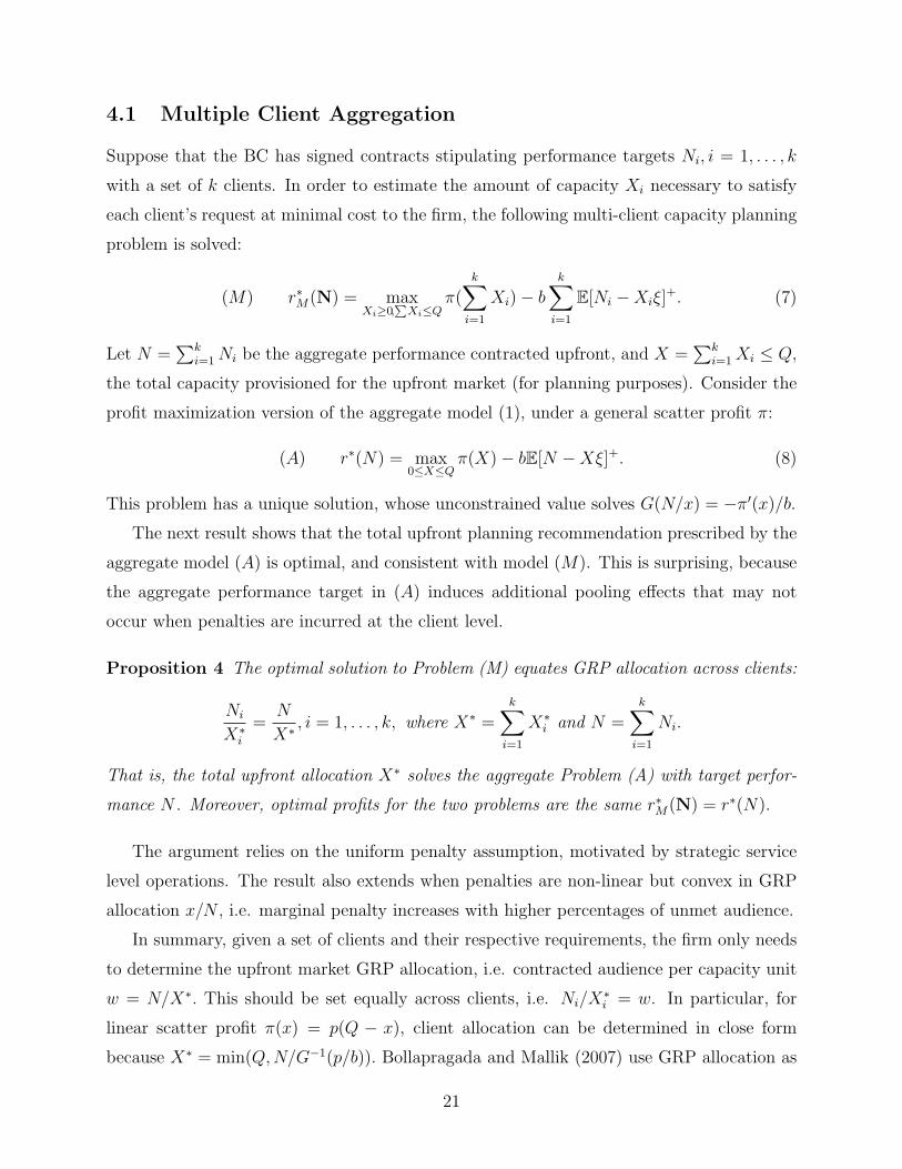
4.1 Multiple Client Aggregation
Suppose that the BC has signed contracts stipulating performance targets Ni, i = 1, . . . , k
with a set of k clients. In order to estimate the amount of capacity Xi necessary to satisfy
each client’s request at minimal cost to the firm, the following multi-client capacity planning
problem is solved:
(M) r∗M(N) = maxXi≥0,
∑Xi≤Q
π(k∑
i=1
Xi)− b
k∑i=1
E[Ni −Xiξ]+. (7)
Let N =∑k
i=1 Ni be the aggregate performance contracted upfront, and X =∑k
i=1 Xi ≤ Q,
the total capacity provisioned for the upfront market (for planning purposes). Consider the
profit maximization version of the aggregate model (1), under a general scatter profit π:
(A) r∗(N) = max0≤X≤Q
π(X)− bE[N −Xξ]+. (8)
This problem has a unique solution, whose unconstrained value solves G(N/x) = −π′(x)/b.
The next result shows that the total upfront planning recommendation prescribed by the
aggregate model (A) is optimal, and consistent with model (M). This is surprising, because
the aggregate performance target in (A) induces additional pooling effects that may not
occur when penalties are incurred at the client level.
Proposition 4 The optimal solution to Problem (M) equates GRP allocation across clients:
Ni
X∗i
=N
X∗ , i = 1, . . . , k, where X∗ =k∑
i=1
X∗i and N =
k∑i=1
Ni.
That is, the total upfront allocation X∗ solves the aggregate Problem (A) with target perfor-
mance N . Moreover, optimal profits for the two problems are the same r∗M(N) = r∗(N).
The argument relies on the uniform penalty assumption, motivated by strategic service
level operations. The result also extends when penalties are non-linear but convex in GRP
allocation x/N , i.e. marginal penalty increases with higher percentages of unmet audience.
In summary, given a set of clients and their respective requirements, the firm only needs
to determine the upfront market GRP allocation, i.e. contracted audience per capacity unit
w = N/X∗. This should be set equally across clients, i.e. Ni/X∗i = w. In particular, for
linear scatter profit π(x) = p(Q − x), client allocation can be determined in close form
because X∗ = min(Q, N/G−1(p/b)). Bollapragada and Mallik (2007) use GRP allocation as
21

a single decision variable in an aggregate upfront market model; our results in this section
validate their approach.
The aggregation result of Proposition 4 can be alternatively interpreted in a context
where a single client requires different performance targets, N, on different shows or periods
(weekly/quarterly weighings, see e.g. Table 10.7 in Talluri van Ryzin 2004). In this case, if
audience is exchangeable, GRP allocation should be balanced across periods, or shows.
4.2 Multi-Client Contracting and Priority Heuristic
In this section, we step back to investigate which upfront clients the BC should accept, among
a given set of client requests, consisting of a target performance Ni and budget Bi, at the
negotiated CPM rate Ci = Bi/Ni. An important limitation of this model is that it focuses
on the firm’s short term profit maximization problem, and thus ignores the impact of current
decisions on customer retention in the context of the firm’s long term profit maximization
problem. Aflaki and Popescu (2007) model the endogenous problem of a service provider
when client demand responds to the cumulative service experience.
We consider a setup where the BC may offer partial fulfilment of client requests, at the
negotiated CPM level Ci. Let yi ∈ Y = [0, 1] be the satisfied fraction of client i’s demand,
and xi the amount of capacity provisioned for client i. Accepting client i increases rev-
enues by Biyi, less potential penalties for unmet performance, but generates scatter market
opportunity cost. Consider the upfront planning profit maximization model:
P = maxyi∈Y
r∗M(N ◦ y) + B′y, (9)
where N ◦ y = (N1y1, . . . , Nkyk) denotes the componentwise product vector of N and y.
The first term stems from the multi-client upfront planning model (M) with contracted
client performance targets Niyi. Proposition 4 reduces this to an aggregate model (A) with
cumulative target N′y. So r∗M(N ◦ y) = r∗(N′y), and the problem can be restated as:
P = maxyi∈Y r∗(N′y) + B′y
= maxN
{r∗(N) + max
N′y=N ;yi∈YB′y
}.
(10)
For any given contracted audience N = N′y, the inner problem is a knapsack model, whose
optimal fractional solution amounts to serving clients in decreasing order of their marginal
profitability, or CPM, Ci = Bi/Ni. Hence this will also be true for the optimal solution of
Problem (10). Client demands should be served as long as they are profitable (i.e. CPM
22

exceeds marginal penalty, so under linear scatter profit Ci ≥ bF (G−1(p/b))) and capacity is
available. Our results have the following implications for client contracting (in absence of
long-term profit considerations):
Proposition 5 Client contracts should be accepted sequentially in decreasing order of marginal
revenue, or CPM Ci = Bi/Ni, as long as they are profitable and capacity is available.
The results in this section remain valid when modeling the opportunity to allocate make-
goods during the broadcasting season, discussed in the next section.
5. Operational Decisions. Make-Goods Allocation
Our results so far focused on static models that provide BCs with decision support during
the upfront market decision process. These capacity provisions are for strategic planning
purposes; they are not actually committed to the client upfront. This section shows how
capacity allocation is operationalized, by extending our basic aggregate capacity planning
model of Section 3 to a multi-period setting. While the focus here is on aggregate upfront
allocation models, our results extend those in Section 4 to handle make-goods allocation
across multiple clients, as argued at the end of this section.
First, the BC decides how much capacity should be committed to clients upfront, with
the provision that this allocation cannot be reduced, but can be increased by subsequently
allocating make goods. Then, as the season starts, and audience ratings unfold, the BC
further decides when and whether to increase initial allocation to under-performing upfront
market client campaigns, by airing make-goods. This decision is continuously traded-off
against immediate scatter market profit opportunities.
Consistent with the broadcasting business cycle, the planning horizon T is assumed to
be one year, discretized into weeks, months or quarters. In this section, ξ captures prior
uncertainty about show popularity; it measures the number of impressions viewing a prime-
time ad. For simplicity of exposition, we assume audiences are i.i.d over time ξt ≡ ξ, but
our results extend for Markovian processes. All comparative statics results extend under
a general performance measure Ψ(x, ξ) that is increasing and concave in x (accounting for
repetition wearout).
23

5.1 Reversible Allocation
Let x0 denote the “irreversible” allocation initially committed to the upfront market. In
each period t ≥ 1, given the remaining target performance Nt, the BC decides how many
additional make-goods xt−x0 to allocate to the upfront market in order to maximize scatter
market profits (realized each period) net of penalties for unmet performance, calculated at the
end of the horizon. The resulting profit (net of contracted upfront client budgets) is denoted
Vt(xt, Nt), and its optimal value Jt(Nt). For an aggregate contracted upfront market target
N, this leads to a dynamic programming model, that optimizes J0(N) = maxx0 J0(x0, N),
given recursively by the following Bellman equation:
Jt(Nt) = maxx0≤xt≤Q
Vt(xt, Nt)
where Vt(xt, Nt) = π(xt) + EJt+1(Nt − ξxt)
and JT (NT ) = −bN+T .
(11)
Because initial allocation x0 is irreversible, it can only limit the firm’s flexibility. It
is easy to see that J0(x0, N) is decreasing in x0, hence minimizing x0 is optimal for J0(N).
This common industry practice, known as gapping, is practically implemented by overstating
performance ratings (i.e. overselling ξ projections). Technically, this allows us to set without
loss of generality x0 = 0 in the corresponding Problem (11). In reality, however, excessive
gapping can negatively affect client relationships on the long run.
The next result characterizes relevant structural properties of the BC’s expected profit,
formalizing the following statements: Expected profit increases with achieved performance,
but its marginal value decreases. Moreover, the value of allocating an extra make-good
decreases with achieved performance, and there is a diminishing marginal rate of substitution
between current make-goods allocation and achieved performance (N − Nt). Finally, the
marginal value of airing an additional make-good (or lowering the performance target by
one unit) is higher later in the horizon.
Lemma 2 The value function has the following properties: (a) Jt is decreasing and concave
in Nt; (b) Vt is jointly concave and has increasing differences in (xt, Nt); (c) Vt(x, N) has
increasing differences in (x, t); (d) Vt has increasing differences in (x,−N) and t.
Recall that a bivariate function g(x, y) has increasing differences in (x, y), if for all x ≤x′, g(x′, y)−g(x, y) is increasing in y. In two dimensions, this is equivalent to supermodularity.
If X is a set of integers, monotone differences amounts to monotonicity of g(x+1, y)−g(x, y).
24
A standard comparative statics result, Topkis’ Lemma, states that if g(x, y) has increasing
differences, then x∗(y) = max argmaxx∈X g(x, y) is increasing in y (Topkis 1998).
A consequence of Topkis’ Lemma and Lemma 2(c), the next result shows that, at any
point in time, the better the achieved performance, the lower the make-goods allocation, all
else equal. Also, the closer the end of the season, the more make-goods need to be aired to
achieve a desired target performance. This is because there are less opportunities to make
up for under-performance in the future.
Proposition 6 The optimal make-goods allocation x∗t (N) is increasing in the remaining
performance target N at any time t, and decreasing in the remaining horizon T − t for any
N ≥ 0, all else equal.
In particular, there exist threshold levels Nt so that additional make-goods are aired at
time t only if the remaining target exceeds the current threshold Nt > Nt. These thresholds
are increasing with achieved performance N −Nt, and over time, all else equal.
5.2 Irreversible Allocation
Depending on the client’s bargaining power, in certain markets make-goods allocation can
be irreversible (e.g. one additional P&G ad will be aired in Friends every week until the end
of the season). This section considers such an irreversible make-goods allocation process.
A similar type of irreversible commitment is common in the study of capacity expansion
strategies (see e.g. Oksendal 2000), leading to similar constraints, but different optimization
models. In our setting, if xt is the total number of slots dedicated to a client at time t,
irreversible allocation means that xt+1 ≥ xt, and effective available capacity at time t + 1
is Q − xt. In practice, sellers do not necessarily resent this limited flexibility, as it often
simplifies their decision making task and induces a more uniform allocation.
The aggregate objective is maxx0 J0(x0, N), with the value function given by the recursive
Bellman equation:
Jt(xt, Nt) = maxxt≤xt+1≤Q
Vt(xt+1, Nt)
where Vt(xt+1, Nt) = π(xt+1) + EJt+1(xt+1, Nt − ξxt+1)
and JT (xT , NT ) = −bN+T .
(12)
Again, gapping considerations suggest that initial upfront allocation should be minimized,
so w.l.o.g. we set x0 = 0. Given a pre-committed allocation x and a remaining target N , the
25

optimal allocation policy is x∗t = x∗t (x, N) = argmaxxt∈[x,Q]Vt−1(x, N). This can be obtained
by projecting the unconstrained optimum, xt(N) = argmaxyVt−1(y, N), on the interval [x, Q].
Proposition 7 The results of Lemma 2 and Proposition 6 under reversible allocation ex-
tend to the irreversible allocation case. Moreover, the optimal irreversible allocation pol-
icy is increasing in the previously committed allocation x, and it is given by x∗t (x, N) =
max(x, min(xt(N), Q)), where xt(N) = argmaxyVt−1(y, N).
The result indicates that the BC should schedule no additional make goods unless the
amount already committed, xt, falls below a certain level, xt+1. Equivalently, the optimal
policy is characterized by threshold levels, Nt+1 = Nt− xt+1µ, so that additional make-goods
are aired only if the remaining target exceeds the current threshold. These thresholds are
increasing with past allocation x, achieved performance N−Nt, and over time, all else equal.
Such structural properties, albeit intuitive, are typically difficult to preserve in a dynamic
and stochastic setting. In particular, the monotonicity of the optimal allocation over time
is a tricky result in the irreversible case, due to the state dependence of the action set
[x, Q]. This excludes the use of standard structural results for dynamic programs with action
independent sets, including Smith and McCardle (2002, e.g. their Proposition 5, p.806).
We conclude this section by observing that the results of Section 4 extend for make-goods
allocation. In particular, the multi-client aggregation result for upfront planning decisions
obtained in Proposition 4 holds for dynamic make-goods allocation. Specifically, the multi-
client make-goods allocation problem reduces to solving the aggregate dynamic program (11)
(respectively (12) in the irreversible case), and allocating the resulting make-goods to clients
in proportion to their remaining targets (see Proposition 8 in the Appendix). Furthermore,
the insights of Proposition 5 remain valid when modeling in (9) the additional recourse
provided by the opportunity to allocate make-goods to clients during the broadcasting season.
We conclude that in order to describe the optimal multiple client solution, it is sufficient to
characterize the optimal revenue and allocation corresponding to the aggregate model.
6. Numerical Results and Heuristics
This section investigates our findings numerically. We first assess the relative error from
ignoring audience uncertainty in static models. Heuristics for dynamic make-goods allocation
are proposed and compared to the optimal policy. We have been able to obtain real data
26

from a major broadcasting network, consisting of audience (number of impressions) per half
hour time interval, for an entire year between 29/04/2007 and 29/04/2008. We also obtained
scatter price data, but in more aggregate form. We first describe how the data was used to
generate inputs into the numerical experiments.
6.1 Input Generation based on Data
The best fit distribution to prime-time (8:00pm-11:00pm) audience data was found to be a
Gamma distribution (followed closely by logistic and student-t distributions). Based on the
data, the average prime-time audience was estimated at µ = 1.5, with a standard deviation
of σ = 0.45, both measured in millions of impressions. We therefore set ξ to follow a
Gamma distribution with shape parameter 11 and scale parameter 0.135. For convenience,
we measure audience in millions of impressions, and dollar amounts in tens of thousands.
The average scatter market price for prime-time spots was estimated at $25,000, with
a standard deviation of $7200. Unfortunately, we did not have access to any sales data,
that would allow us to estimate a demand function. For the numerical analysis, we use an
iso-elastic scatter market demand function d(p) = ap−η, with elasticity η > 1. This leads to
a profit model π(x) = ap1−η = p0(Q − x)1−1/η, where p0 = a1/η corresponds to the profit
from one unit capacity available to the scatter market. We set η = 1.5, and used the average
estimate based on the data, to set p0 = 2.5 (in tens of thousand of dollars). Our insights are
robust with respect to the elasticity η > 1, and other scatter profit models, including linear
and log-demand.
We report results for various penalty levels, b, from 10 to 125 (in tens of thousands
of dollars), corresponding to service levels of 75% to 98% (see Section 3.1). As expected,
penalty values usually much exceed the scatter market CPM, which in our case is at most
p0/µ = $16.7 per thousand impressions; this value is realistic for the network at hand.
For make-goods allocation, we focused on a one year, four-quarters horizon (T = 4),
i.e. make-goods allocation is assumed to be revised once every three months. The capacity
Q, corresponding to the total number of prime-time ads for a quarter, is set to Q = 4200.
This is justified by information provided by the network: the number of 30 second ads per
hour in prime-time ranges between 16 and 20, amounting to a total capacity of 4008-5040
prime-time ads in 12 weeks (or one quarter).
The target audience N was varied over the range from 0 to 25000 million impressions.
This range was chosen based on the expected audience (for the total number of ads available)
27

over the entire horizon, which is N0 = µ ·Q ·T = 25200 million. Empirical evidence suggests
that about 80% of a network’s average ratings are sold upfront. For values N ≥ N0, all
policies appear to behave very similarly, by allocating all the capacity to the upfront.
Our extensive numerical studies, for a wide range of meaningful numerical values, indicate
that the results presented here are representative and robust. The numerical results are also
scalable, in the sense that similar patterns are observed if make-goods allocation decisions
are made with a different frequency, and capacity is adjusted accordingly (e.g. for one month
instead of one quarter periods, the total prime-time capacity is in the order of Q = 1400
ads, and N0 = 8400 million impressions).
In the realistic context of this data, we first briefly assess the impact of uncertainty in
static upfront allocation (ignoring make-goods), as identified in Lemma 1. Table 2 below
shows the relative error between the capacity allocation obtained based on a deterministic
audience, xd = min{Q, N/(Tµ)}, and the optimal static upfront allocation, x∗, obtained
by solving the stochastic audience model (8). The average relative allocation error, ∆x, is
calculated by averaging over N the percentage gap x∗−xd
xd. We also report the corresponding
average relative static profit error ∆r, calculated by averagingr∗(N)− r(xd, N)
r∗(N)over N ,
where r(x, N) = π(x)− bE[N − xξ]+ and r∗(N) = max0≤x≤Q r(x, N), as defined in (8). The
results suggest that, by ignoring audience uncertainty, the deterministic approach largely
under-allocates capacity to the upfront, and the error deteriorates with higher service levels.
Table 2. Static allocation error for various penalties, and corresponding service levels.
Penalty level (b) 10 15 20 30 70 125Relative allocation error (∆x) 32% 35% 37% 39% 45% 49%Relative profit error (∆r) 32% 66% 138% 144% 299% 605%
6.2 Heuristics for Dynamic Make-Goods Allocation
The practical inconvenience of solving the make-goods allocation dynamic program to op-
timality (due to the curse of dimensionality) motivates us to study several intuitive and
efficient heuristics for make-goods allocation, described next.
A myopic policy reduces the visibility of the decision maker to a shorter horizon, by
introducing sub-targets for corresponding sub-horizons. For clarity, we consider the extreme
situation where each period is a sub-horizon and the target N is initially divided uniformly
across periods. The static myopic (s-myopic) policy allocates a constant amount of capacity
28

each period, corresponding to a per period target N/T, as long as this does not exceed the
actual remaining target. Concretely, in each period t, the s-myopic allocation xs−myopic solves
the static model (1) with general scatter profit π, and target Nt = min(N/T, Nt), where Nt
is the total actual remaining target. A natural improvement over this heuristic is the myopic
policy, which periodically updates the target for the next period, by spreading the actual
remaining audience target uniformly across the remaining horizon, so Nt = Nt/(T − t).
The static policy provides the corresponding optimal open-loop policy, deciding alloca-
tions for each period before audience realizations are revealed. This model is analogous to the
multi-stage model (CT ) of Section 3.3 with non-linear scatter market profit. Proposition 3
insures that the static policy allocates the same amount of make-goods xstatic in each period.
Specifically, the static solution solves a non-linear scatter profit version of model (1), with
target N and cumulative audience distribution equal to the convolution ξ(T ) = ξ1 + · · ·+ ξT ,
where ξi, i = 1, . . . , T are i.i.d. with the same distribution as ξ. That is, xstatic solves:
maxx∈[0,Q]
Tπ(x)− bE[N − xξ(T )
]+.
By design, the static policy is implicitly also a valid heuristic for the irreversible model. A
natural improvement on the static policy is obtained by resolving the static policy in each
period, based on the remaining target: this is called the r-static heuristic.
The Certainty Equivalent Control (CEC) heuristic approximates the profit-to-go by set-
ting the audience in all remaining periods to its expected value Eξ = µ (see e.g. Bert-
sekas 2008). By ignoring audience uncertainty, the CEC policy is likely to capture, at an
aggregate level, what is currently done in practice (where deterministic audience models
are used). Specifically, in each period, the CEC solves the deterministic concave problem:
max{∑T
i=t π(xi) − bZ | Z ≥ Nt − (∑T
i=t xi)µ, Z ≥ 0 and 0 ≤ xi ≤ Q, t ≤ i ≤ T}.Concavity of π implies that, at an optimal solution, the allocation is uniform and equal to
x∗t = max{argmax(π(x) + xbµ),Nt
(T − t + 1)µ}. This is the amount allocated by the CEC
policy in period t. The policy re-solves periodically the corresponding deterministic approx-
imation, after updating the remaining target based on realized audience.
Another heuristic that relies on deterministic audience is the minimal postponement pol-
icy, which prioritizes allocation to the upfront market, while approximating future audience
by its mean. Only once the client target is met, the policy starts selling to the scatter mar-
ket. Specifically, it sets xt = min(Q,Nt/µ), as long as Nt > 0. One can similarly define a
29

maximum postponement policy. For conciseness, these policies are not reported due to their
relatively poor performance.
2 4 6 8 10 12 14 16 18 20−10
−5
0
5
10
15
Remaining target, N
Profit−to−go
5 10 15 20 250
0.5
1
1.5
2
2.5
3
3.5
4
Remaining target, N
Capacity Allocation
r−static
static
u−myopic
myopic
Optimalreversible
CEC
CEC
static
myopic
Optimalreversible
Optimalirrreversible
Optimalirrreversible
Figure 1: Heuristic and optimal value functions, and corresponding allocation policies, at t = 1, relativeto the target N , for T = 4 and b = 30.
The first graph in Figure 1 compares numerically the performance of these policies in
terms of total expected profits (calculated by Monte Carlo simulation) at the beginning of
a four quarter horizon T = 4. Table 3 gives the relative value function error, for different
values of the penalty b, averaged over initial values of N . For a given heuristic h, the average
relative error ∆h is defined as the percentage optimality gap∣∣∣Jrev−Jh
Jrev
∣∣∣, averaged across the
relevant values of N ; here Jrev is the optimal expected profit under the reversible regime.7 In
our experiments, the r-static policy achieved consistently and by far the best value function
approximation, with a relative error (with respect to the optimal reversible policy) ranging
between 0.2% and 0.5% (it is not distinguishable from the optimal policy on the graph). It
is followed by the myopic policy, with a relative error ranging between 1.75% and 5%. The
performance of these two heuristics improves as the remaining target N increases. The profit
relationships depicted in Figure 1, as well as the policy rankings described in Table 3 are
robust for all practically relevant service levels (i.e. penalty values b ≥ 10). The static policy
is the only heuristic among those considered here that is also feasible for the irreversible
7Relative profit performance is actually much better than Table 3 reports, because it should also considerthe upfront budget B, omitted by our value function calculations. To give an idea of the magnitude of B,in 2005, the six biggest networks in the US alone collected over $9 billion in upfront revenues, that is 1/7 ofthe $63 billion TV advertising market, according to TNS. So, accounting for B, relative profit performanceswould be at most 6/7 = 86% of reported values.
30

model, with respect to which it achieves a relative error in the order of 5%.
Table 3. Average relative error ∆h for various heuristics and penalty levels
Heuristic b = 10 b = 15 b = 20 b = 30 b = 70 b = 125static 26.75% 24.79% 21.07% 39.76% 42.04% 35.07%r-static 0.53% 0.48% 0.22% 0.32% 0.39% 0.19%s-myopic 7.86% 8.00% 7.29% 11.51% 11.76% 9.82%myopic 1.73% 2.05% 2.02% 3.89% 5.06% 4.56%CEC 67.72% 88.38% 92.18% 275.29% 512.06% 519.82%
The second graph in Figure 1 displays the allocation of each heuristic at the beginning
of a four period horizon, as a function of the target audience N , calculated by Monte Carlo
simulation. The figure suggests the following allocation ordering: xCEC ≤ xirrev ≤ xstatic =
xd−static ≤ xrev ≤ xmyopic = xs−myopic. Our numerical results suggest that this is consistent
for all practical levels of b. We provide an intuitive argument for this. Because the irreversible
policy can (only) increase initial allocation in the future, it is expected to set a lower initial
allocation than the static one. Relative to the reversible regime, the static policy does not
have the opportunity to decrease make-goods allocation over time, so it sets a lower first
stage allocation (to avoid unrewarded over-performance). The myopic policies neglect the
opportunity of correcting performance in future allocations, hence over-allocate relative to
the optimal reversible policy. The CEC policy allocates by far the least amount of capacity,
because it ignores the risk of audience uncertainty.
Our numerical investigations indicate that periodically resolving static and myopic poli-
cies, based on the simple static upfront allocation model (1), can provide a surprisingly good
approximation for the complex dynamic make-goods optimization problem. In addition,
simple static policies provide good approximations for irreversible regimes. Incidentally,
myopic policies have also been noted to perform well for certain random yield models (see
e.g. Sepheri et al. 1986, Bollapragada and Morton 1999), but this is not a robust result,
particularly for periodic review (see e.g. Rajaram and Karmakar (2002)).
We conclude that ignoring audience uncertainty for make-goods allocation can lead to
relatively poor performance (e.g. the CEC policy), compared to simple policies that use
audience uncertainty information (r-static and myopic). This underlines the importance of
considering audience uncertainty in the dynamic make goods allocation problem, which is
currently not the case in practice.
31
7. Conclusions
This paper focuses on capacity planning decisions across upfront and scatter markets in
the presence of audience uncertainty. We propose stylized models that take into account
important elements of the media revenue management problem and provide insights for
operational decisions. From a modeling standpoint, an important contribution is that we
specifically account for prior uncertainty about audience ratings. We also specifically model
the trade-off between spot and upfront allocation to multiple clients.
Our results provide insight into how much capacity should be planned for upfront vs.
scatter markets when ratings are uncertain. We also make recommendations for dynamic
make-goods allocation during the broadcasting season. Our results suggest the following
procedure for upfront client contracting, capacity planning and make-goods allocation:
1. Serve clients in decreasing CPM order; plan capacity requirements for upfront clients
in proportion to requested audience (total capacity requirement for the upfront market
can be estimated using model (A)).
2. Allocate minimal initial capacity to clients upfront (gapping);
3. Obtain total make-goods allocation by solving the (one-dimensional state) dynamic
programming Problem (11) (or e.g. a r-static or myopic heuristic) with aggregate
target performance; its value function represents the expected year-end profit (net of
client budgets).
4. Allocate make-goods to clients in proportion to their remaining performance targets,
i.e. by balancing GRP allocation.
Given that current industry practice is to make such decisions qualitatively, this procedure
can provide insights for capacity planning. In particular, the aggregation results have the
potential to facilitate a centralized decision process.
We also provide structural results characterizing sensitivity of profits and capacity allo-
cation to model parameters. Our analytical and numeric results suggest that models based
on deterministic audience have a tendency to underestimate the capacity allocation required
to hedge against audience uncertainty. In addition, while it is expected that more popular
shows would require lower capacity allocation to satisfy a certain demand, this is not always
the case (it depends on the nature of audience uncertainty). Our numerical assessment of
32

various heuristics for make-goods allocation confirm the importance of modeling uncertainty
in the media planning task. Specifically, periodically resolving static and myopic policies,
which account for audience uncertainty, significantly outperforms policies based on deter-
ministic audience approximations.
Our models can also be useful in other settings where the value of supply is uncertain,
and/or the firm serves dual markets. For instance, in manufacturing with random yield, a
firm with limited resources and uncertain production rate (e.g. machine or workforce reliabil-
ity) honors both key accounts with long term contracts and small clients with opportunistic
contracts (alternatively, our scatter market opportunity cost corresponds to direct produc-
tion cost). Similarly, non-profit organizations (NPO) afford to sustain pro bono service to
a mission market by often offering similar paid services to distinct markets, that share the
same limited facilities (e.g. hospitals) powered by uncertain resources (e.g. volunteers).
Here, the mission market corresponds to our upfront market and the paying market to our
scatter market. de Vericourt and Lobo (2008) investigate revenue management for NPOs.
There are multiple facets of the media revenue management problem that this paper
leaves to be explored, including strategic decisions, such as pricing and contract design, as
well as tactical scheduling and client-to-show matching. The latter have been studied in the
literature using deterministic combinatorial models (Bollapragada et al. 2002, Bollapragada
and Garbiras 2004, Zhang 2006, Kimms and Muller-Bungart 2007). An interesting question
for future research is to characterize the optimal allocation across multiple shows, with
heterogeneous audience uncertainty, especially in a dynamic setting. This involves solving
a multi-period stochastic portfolio-type problem. Banciu et al. (2007) investigate bundle
pricing strategies for TV ads on the scatter market. Contract design is an interesting area,
where the industry is quite sophisticated, managing a variety of flexible products, such as
option-cutbacks (revised planning due to client’s budget cuts) or callable products (lower
rates with the option of recalling the slot for a higher paying customer). The latter, and
their value for standard B2C revenue management are investigated in Gallego et al. (2008).
Finally, it is an irreversible fact that audience is moving online, where capacity is more
complex, dynamic and customizable, leading to different contractual terms (e.g. pay per
click vs CPM – pay per view). Araman and Fridgeirsdottir (2008) investigate a queuing
model for online advertising revenue management.
33
Acknowledgments
The authors would like to thank Paul Kleindorfer for insightful comments and suggestions.
Several industry experts are gratefully acknowledged for insightful exchanges about practi-
cal aspects of media planning and revenue management, including Srinivas Bollapragada,
Michael Chigirinskiy, Monique Garnier, Ahmet Kuyumcu, Robert Phillips, Antoine Tacon-
net, Abraham Toledano, Loren Williams and Graham Young. The second author gratefully
acknowledges funding from the Booz &co. Chair in Revenue Management at INSEAD.
Appendix (Proofs)
Proof of Proposition 2 (Audience sensitivity)
(a) The first order condition (4) can be restated as bGξ(z)(N/x)/µ(z)− p(z)/µ(z) = 0. The
assumptions imply that the left hand side is decreasing in z, hence so is x∗(z).
(b) Proposition 1 suggests that the optimal (unconstrained) allocation solves:
G(N/x, z) = p(z)/b, where G(N/x, z) = E[ξ(z)I(ξ(z) ≤ N/x)] =
∫ N/x
0
yf(y, z)dy. (13)
Here f(y, z) = f0(y − µ(z)) denotes the density function of ξ(z). This is decreasing in z for
y ≤ µ(z), because f0 is unimodal with non-negative mode. Thus, G(N/x, z) is decreasing in
z for x ≥ N/µ(z).
The condition on b implies x∗(z) > N/µ(z). Monotonicity of x∗(z) follows because p(z)
is increasing in z and G(N/x, z) is decreasing x, and decreasing in z for x ≥ N/µ(z).
(c) Recall that ξ1 �lr ξ2 if and only if the ratio of the corresponding densities f2(u)f1(u)
is
increasing in u. The density of ζ is h(u) = u/µf(u), where f is the density of ξ (see e.g. the
proof of Remark 1). Therefore ξ1 �lr ξ2 if and only ζ1 �lr ζ2. Because ξ(z) is stochastically
increasing in z in lr-order, it follows that ζ(z) is also increasing in z in lr-order, and hence
in first order. The latter, together with P(θ(z) ≥ x) = P(ζ(z) ≤ N/x) (again by the proof of
Remark 1), implies that θ(z) is decreasing in z in first order dominance. Therefore, by (5),
the critical fractile solution, x∗(z), is decreasing in z.
(d) The result follows from part (c) because, for all the distributions listed in the proposi-
tion, the order of parameters that characterizes first order dominance also induces likelihood
ratio ordering (see e.g. Tables 1.1 and 1.2 in Muller and Stoyan, 2002, pages 62-63).
34
Proof of Proposition 3 (Multi-stage planning)
The proof relies on the following lemma (Muller and Stoyan 2002, Theorem 8.2.3):
Lemma 3 Suppose that u is a decreasing convex function and ωi are exchangeable. The
optimal solution y∗ ∈ Rk to the problem min1′y=q, y≥0
Eu(y′ω) satisfies y∗i = q/k for all i.
Problem (CT ) can be written as
min0≤xi≤Q
p1′x + bE[N − x′ξ]+ = min0≤q≤kQ
pq + bZ(q), (14)
where Z(q) = min0≤xi≤Q
E[N − x′ξ]+ (15)
1′x = q.
By Lemma 3, the optimal solution of Problem (15) without the capacity constraints xi ≤ Q
is x∗i (q) = q/k, i = 1, . . . , k. For q ≤ kQ, x∗i (q) = q/k ≤ Q, so this solution is feasible, hence
also optimal for Problem (15) with capacity constraints. Therefore, Problem (14) becomes:
min0≤q≤kQ
pq + bE[N − (q/k)k∑
i=1
ξi]+. (16)
This is precisely Problem (1) with target N, audience distribution ξ =∑k
i=1 ξi
kand capacity
kQ. Letting q∗ denote its optimal solution, the optimal allocations in the original problem
(CT ) must equal x∗i (q∗) = q∗/k, i = 1, . . . , k, which proves the desired result.
Proof of Proposition 4 (Upfront planning aggregation)
For any feasible multi-client allocation X = (X1, . . . , Xk), the corresponding aggregate allo-
cation X =∑k
i=1 Xi is feasible for model (A), and the corresponding penalty cost can not
be higher in the aggregate model (because of pooling effects∑
a+i ≥ (
∑ai)
+). Hence,
r∗M(N) = maxXi≥0,
∑Xi≤Q
π(k∑
i=1
Xi)− bk∑
i=1
E[Ni −Xiξ]+ ≤ max
0≤x≤Qπ(x)− bE[N − xξ]+ = r∗(N).
(17)
Consider now the optimal solution x∗ of the aggregate Problem (A), and define X∗i =
Nix∗/N, i = 1, . . . , k. This is feasible to Problem (M), and satisfies
∑i X
∗i = x∗ and∑k
i=1 E[Ni −X∗i ξ]+ = E[N − x∗ξ]+. So x∗ achieves the same profit as the optimal aggregate
model profit r∗(N), so it is optimal for model (M) (and unique by concavity of the objective).
Moreover, the optimal profits of the multi-client and aggregate problems are equal.
35

Proof of Lemma 2
The terminal value function JT is decreasing and concave in NT . Together with concavity of
πt, this implies that VT−1 is jointly concave and has increasing differences. By induction we
obtain that Vt is jointly concave and has increasing differences in (x, N) and Jt is decreasing
concave in Nt implying (a) and (b).
Parts (c) and (d) follow by writing Vt−1(x, N)−Vt(x, N) = E[Jt(N−xξ)−Jt+1(N−xξ)].
Concavity (hence decreasing differences) of Jt+1 implies that, for any realization z of ξ, the
function inside the expectation below is increasing in (N,−x):
maxx0≤y≤Q
π(y) + E[Jt+1(N − xz − yξ)− Jt+1(N − xz)].
Preliminary Technical Lemmas for Section 5.2
We next present two general technical lemmas that are used to prove the results in this
section. The generality of the presentation allows to easily extend the proofs for general
performance metrics Ψ(x, ξ), validating the claims made in the Introduction. specifically,
the proof for Ψ(x, ξ) uses Lemma 4 b) and c), and the induction in Proposition 7 should be
conducted simultaneously for all increasing concave functions Ψ(x, ξ), in order to achieve
the last step of the proof.
Lemma 4
(a) f concave implies g(x, y) = f(x + y) is concave and has decreasing differences.
(b) f concave and h increasing implies g(x, y) = f(h(x) + y) has decreasing differences.
(c) f increasing concave and h concave implies g(x, y) = f(h(x) + y) joint concave.
(d) If f(x, y) has decreasing differences in (x, y) and is concave in y and h(x) is increasing
then g(x, y) = f(x, h(x) + y) has decreasing differences in (x, y).
The proof follows from the definitions. Analogous conditions for increasing differences ob-
tain from the fact that g(x, y) has increasing differences if and only if g(−x, y) has decreasing
differences if and only if g(x,−y) has decreasing differences.
Lemma 5 (a) The function g(x) = maxy∈Sx
f(x, y) is decreasing in x if f(x, y) is decreasing in
x and Sx′ ⊆ Sx for all x ≤ x′.
(b) The function g(x) = maxy∈Sx
f(x, y) is concave in x if f(x, y) is jointly concave in (x, y)
and the set {(x, y); y ∈ Sx} is convex.
36

(c) The function g(x, y) = maxv∈[x,Q] f(v, y) has decreasing (increasing) differences in
(x, y) if f(v, y) has decreasing (increasing) differences in (v, y).
The proof of the first part is trivial. The second and third parts follow directly from
Porteus (2002), Theorem A.4 and Theorem 8.2, respectively.
The next result extends Lemma 2 under irreversible commitment.
Lemma 6 (Value function properties) (a) Jt is decreasing in Nt and in xt; (b) Jt is
jointly concave in (xt, Nt); (c) Jt has increasing differences in (xt, Nt) and Vt has increasing
differences in (xt+1, Nt); (d) Vt(x, N) and Jt(x, N) have increasing differences in (x, t).
Proof: (a) Monotonicity is easily proved by induction and Lemma 5 (a). The base case
is trivial, transitions are linear and the profit per stage is state-independent.
(b) We show by backward induction that Jt is jointly concave in (xt, Nt). The base case
is satisfied because JT (x, NT ) = −bN+T is (jointly) concave. Suppose Jt+1 is jointly concave,
so Jt+1(xt+1, Nt − ξxt+1) is jointly concave in (xt+1, Nt), hence so is Vt(xt+1, Nt). By Lemma
5 (b), Jt is jointly concave in (xt, Nt).
(c) We prove both statements in parallel by induction. The base case is trivial. Because
Jt+1 has increasing differences, by Lemma 4 (d), we obtain that EJt+1(xt+1, Nt−ξt+1xt+1) has
increasing differences in (xt+1, Nt), hence the same holds for Vt. Finally, increasing differences
and concavity of Vt implies increasing differences of Jt by Lemma 5 (c).
(d) The result follows independently from the proof of Proposition 7 below.
Proof of Proposition 7
The optimal allocation policy is x∗t = x∗t (x, N) = argmaxxt∈[x,Q]Vt−1(x, N), which can be
obtained by projecting the unconstrained optimum xt(N) = argmaxyVt−1(y, N), on the
interval [x, Q]. This shows the second part of the statement.
Monotonicity of the optimal policy in N and x follows from Lemma 6 (c) together with
Topkis’ Lemma. It remains to show monotonicity with time. We show by backwards induc-
tion the following three statements in parallel:
[J-t] Jt(x, N − xz)− Jt+1(x, N − xz) decreasing in x for all N, z ≥ 0.
[V-t] Vt−1(x, N)− Vt(x, N) is decreasing in x for all N ≥ 0.
[x-t] x∗t (x, N) ≤ x∗t+1(x, N) for all N, x ≥ 0.
The base case [J-(T-1)] is obviously true. The following is true for all t:
37

[J-t] ⇒ [V-t] because Vt−1(x, N)− Vt(x, N) = E[Jt(x, N − xξ)− Jt+1(x, N − xξ)].
[V-t] ⇒ [x-t] by Topkis’ Lemma.
It remains to show [x-t] ⇒ [J-(t-1)], i.e. the following function decreases in x, ∀N, z ≥ 0 :
j(x) = Jt−1(x, N − xz)− Jt(x, N − xz)
= Vt−1(x∗t (x, N − xz), N − xz)− Jt(x, N − xz) (18)
= maxx≤y≤Q
π(y) + E[Jt(y, N − xz − yξ)− Jt(x, N − xz)]. (19)
Depending if it is optimal to allocate additional make goods at time t + 1, we obtain:
Jt(x, N − xz) =
{Jt(0, N − xz), if x∗t+1(x, N − xz) > x (case 1)Vt(x, N − xz), if x∗t+1(x, N − xz) = x (case 2).
(20)
Case 1: To show that j(x) is decreasing in x, by Lemma 5 a), it is enough to show that
the following function (inside the expectation in (19)) is decreasing in x for all y, z, v ≥ 0:
g(x) = Jt(y, N − xz − yv)− Jt(x, N − xz) = Jt(y, N − xz − yv)− Jt(0, N − xz)
= [Jt(y, N − xz − yv)− Jt(y, N − xz)] + [Jt(y, N − xz)− Jt(0, N − xz)]. (21)
Indeed, by Lemma 6, the first difference is decreasing in x by concavity of Jt in the second
argument, and the second difference is decreasing in x by increasing differences of Jt.
Case 2: We have x ≤ x∗t (x, N − xz) ≤ x∗t+1(x, N − xz) = x, by the induction hypothesis
[x-t]. Therefore x∗t (x, N − xz) = x. This together with (20) allows to rewrite (18) as
j(x) = Vt−1(x, N − xz)− Vt(x, N − xz) = E[Jt(x, N − xz − xξ)− Jt+1(x, N − xz − xξ)].
The right hand side is decreasing in x because the function inside the expectation Jt(x, N −x(z + v))− Jt+1(x, N − x(z + v)) is so for any z, v ≥ 0, by [J-t]. This concludes the proof.
Multi Client Make-goods Aggregation
The dynamic multi-client make-goods allocation problem can be formulated as:
JMt (Nt) = max
x0≤xt;1′xt≤QV M
t (xt,Nt)
where V Mt (xt,Nt) = π(1′xt) + EJM
t+1(Nt − ξxt)
and JMT (NT ) = −b1′N+
T ,
(22)
where 1 is the vector of ones, and x0,xt,Nt are vectors denoting, for each client, the initial
irreversible allocation, the total allocation at time t, and the remaining target at time t,
respectively. Our next result shows that model (22) reduces to solving the corresponding
aggregate model (11), resulting in a dynamic program with a one-dimensional state variable.
38

Proposition 8 The dynamic-make goods multi-client allocation Problem (22) is equivalent
to the corresponding aggregate Problem (11) with target performance Nt = 1′N+t , in that:
(1) the value functions of the two problems are equal, JMt (Nt) = Jt(Nt), and (2) the total
optimal make-goods allocation under model (22) equals the optimal make-goods allocation
under model (11), 1′x∗t = x∗t . Furthermore, in each period, make-goods x∗i,t are optimally
allocated to clients in proportion to their remaining performance targets N+i,t, i.e. by balancing
GRP allocation. The results extend for irreversible allocation.
Proof: The proof is by induction. The base case is given by Proposition 4, so, in
particular, x defined by xi/Ni = X∗/N is optimal to the multi-client model, and JMT−1(N) =
JT−1(N).
Now, assuming the result is true for t + 1, we show that it also holds for t. Assume
wlog that N ≥ 0; otherwise replace N by its positive part, because JMt (N) = JM
t (N+). For
X = 1′x we have:
V Mt (x,N) = π(1′x) + EJM
t+1((N− ξx)+)= π(X) + EJt+1(1
′(N− ξx)+) (induction step)≤ π(X) + EJt+1((N − ξX)+). (monotonicity of Jt)
(23)
Therefore,JM
t (N) = max0≤x;1′x≤Q
V Mt (x,N)
= max0≤X≤Q
π(X) + EJt+1(1′(N− ξx)+)
≤ max0≤X≤Q
π(X) + EJt+1((N − ξX)+)
= Jt(N).
(24)
Consider the optimal allocation X∗ that optimizes Jt(N) above, and let x so that xi/Ni =
X∗/N, for all i with Ni > 0. This is feasible and achieves (24) with equality, hence it is an
optimal solution to the multi-client model, and the two value functions are equal. This
concludes the proof of the reversible case.
The aggregation result for irreversible allocation follows the same lines as the reversible
allocation case. The only additional condition to verify is feasibility of the multi-client
solution provided by the equal GRP rule. We need to show that the lower bounds imposed by
the irreversible allocation are satisfied. In a balanced GRP solution,X t
i
N ti
=X t
j
N tj
for N ti , N
tj > 0,
soX t
i
N ti − zX t
i
=X t
j
N tj − zX t
j
, for any realization z ≥ 0 of ξ, implyingX t
i
X tj
=N t+1
i
N t+1j
=X t+1
i
X t+1j
. This
shows that allocation increases proportionally over time for each unsatisfied client, so the
irreversibility constraints are met. Hence the multi-client problem reduces to the aggregate
case under irreversible commitment.
39

References
Aflaki, S., I. Popescu 2008. Service Dynamics under Repeated Interactions. Working paper.
Alvarado, C. 2007., Revenue Management for the Inventory Optimization of Television
Azteca, Television Azteca external communication document.
Araman, V.F., K. Fridgeirsdottir 2008. Online advertising: A revenue management ap-
proach. Working paper.
Araman, V.F., O. Ozer 2005. Capacity and inventory management in the presence of a
long-term channel and a spot market, Working paper.
Banciu, M., E. Gal-Or, P. Mirchandani, 2007. A Mixed-Bundling Pricing Strategy for the
TV Advertising Market, Working paper, Katz School of Business, University of Pittsburgh
Bertsekas, D. 2007. Dynamic Programming and Optimal Control. Athena Scientific.
Bollapragada, S., H. Cheng, M. Phillips, M. Garbiras. 2002. NBC’s optimization systems
increase revenues and productivity. Interfaces 32 (1) 47-60.
Bollapragada, S., M. Garbiras. 2004. Scheduling commercials on broadcast television. Op-
erations Research 53 (3) 337-345.
Bollapragada, S., S. Mallik. 2007. Managing the inventory of commercial airtimes in broad-
cast television. Working paper.
Bollapragada, S., T.E. Morton. 1999. Myopic heuristics for the random yield problem. Op-
erations Research 47 (5) 713-722.
de Vericourt, F., M. S. Lobo. 2008. Resource and Revenue Management in Nonprofit Oper-
ations. Operations Research, forthcoming.
Elmaghraby, K., P. Keskinocak. 2003. Dynamic pricing in the presence of inventory consid-
erations. Management Science 49(10) 1287-1309.
Gallego, G., S.G. Kou, R. Phillips. 2008. Revenue Management of Callable Products. Man-
agement Science 54(3) 550-564
Grosfeld-Nir, A., Y. Gerchak. 2004. Multiple lotsizing in production to order with random
yields: Review of recent advances. Annals of Operations Research 126 43-69.
Gupta, D., W. L. Cooper. 2005. Stochastic comparisons in production yield management.
Operations Research 53 (2) 377-384.
Guu, S.M., A. X. Zhang. 2003. The finite multiple lot sizing problem with interrupted geo-
metric yield and holding costs. European Journal of Operational Research 145(3), 635-644.
Kanetkar, V., C.B. Weinberg, D.L. Weiss. 1992. Price Sensitivity and Television Advertising
40

Exposures: Some Empirical Findings. Marketing Science 11 (4) 359-371.
Kimms, A., Muller-Bungart, M., 2007. Revenue management for broadcasting commercials:
the channel’s problem of selecting and scheduling the advertisements to be aired. Interna-
tional Journal of Revenue Management 1(1) 28 - 44.
Kleindorfer, P., Wu, D.J., 2003. Integrating long-term and short-term contracting via B2B
exchanges for capital-intensive industries. Management Science 49 (11) 1597-1615.
Lodish, L.M., M. Abraham, S. Kalmenson, J. Livelsberger, B. Lubetkin, B. Richardson,
M.E. Stevens. 1995. How TV Advertising Works: A Meta-Analysis of 389 Real World Cable
TV Advertising Experiments. Journal of Marketing Research 32 125-139.
McCardle, K., K. Rajaram, C. S. Tang. 2004. Advance Booking Discount Programs Under
Retail Competition. Management Science, 50 (5) 701 - 708.
Metheringham, R. A., 1964, Measuring the Net Cumulative Coverage of a Print Campaign,
Journal of Advertising Research, 4 23-28
Muller, A., D. Stoyan. 2002. Comparison Methods for Stochastic Models and Risks. Wiley.
Porteus, E. L. 2002. Foundations of Stochastic Inventory Theory. Stanford Business Books.
Prekopa, A. 1995. Stochastic Programming. Kluwer Academic Publishers.
Oksendal, A. 2000. Irreversible investment problems. Finance Stochastics 4 223-250.
Rajaram, K., U.S. Karmakar. 2002. Product Cycling With Uncertain Yields: Analysis And
Application To The Process Industry. Operations Research 50(4): 680-691.
Sepehri, M., E. A. Silver, C. New. 1986. A Heuristic for multiple lotsizing for an order under
variable yield. IIE Transactions 63-69.
Shih, 1980. Optimal inventory policies when stockouts result from defective products. Int.
J. Production Research 18(6), 677-685.
Smith, J. E., K.E. McCardle 2002. Structural Properties of Stochastic Dynamic Programs,
Operations Research 50 796-809.
Talluri, K., G. van Ryzin. 2004. The Theory and Practice of Revenue Management. Kluwers
Academic Publishers.
Topkis, D. M. 1998. Supermodularity and Complementarity. Princeton University Press.
Wu, D. J., P. Kleindorfer. 2005. Competitive options, supply contracts and electronic mar-
kets. Management Science 51 (3) 452-466.
Yang, S., J. Yang, L. Abdel-Malek. 2007. Sourcing with Random Yield and Stochastic
Demand. Computers and Operations Research 34 (12) 3682-3690
Yano, C., H. L. Lee. 1995. Lot sizing and random yields: A review. Operations Research
41

43(2) 311-334.
Zhang, X. 2006. Mathematical Models for the Television Advertising Allocation Problem.
IJOR 1 (3) 302-322.
42
Top Related