


Languages
Pages
Legal


Media and Crime Perceptions: Evidencefrom Mexico
Aurora Alejandra Ramırez-Alvarez∗
Brown University
Abstract
This paper examines whether individuals’ crime perceptions and crime avoid-
ance behavior respond to changes in crime news coverage. I use data from Mexico,
where major media groups agreed to reduce coverage of violence in March 2011.
Using a unique dataset on national news content and machine learning techniques,
I document that after the Agreement, crime news coverage on television, radio, and
newspapers decreases relative to the national homicide rate. Using survey data, I
find robust evidence that crime perceptions respond to this change in content. After
the Agreement, individuals with higher media exposure are less likely to report that
they feel insecure and that their country, state, or municipality is insecure, relative
to individuals with lower media exposure. However, I show that these changes in
crime perceptions are not accompanied by changes in crime avoidance behavior (i.e.
no longer going out at night for fear of being a victim of crime), or at least that
effects are much smaller.
Keywords: mass media; persuasion; crime perception
JEL codes: D83, K42, L82
∗I am deeply indebted to Brian Knight, Jesse Shapiro, and Daniel Bjorkegren for their guidance,constant support, and encouragement. I also thank Joseph Acquah, Anna Aizer, Guillermo Alves, PedroDal Bo, Andrew Foster, John Friedman, Margarita Gafaro, Anja Sautmann, Glenn Weyl, and seminaraudiences at Banco de Mexico, Brown University, El Colegio de Mexico, Universidad de Guanajuato,and Rutgers-Newark for helpful suggestions and conversations. I am greatly indebted to AlejandraMolina, who arranged several meetings with Mexican policy makers. All remaining errors are my own.Address: Department of Economics, Brown University, 64 Waterman St., Providence, RI 02912. E-mail:aurora ale [email protected]
1

1 Introduction
Crime is a major concern in Mexico. According to survey data, around 70% of
Mexicans say crime is one of the three most important problems in the country. In fact,
in the survey, crime is listed as the nation’s biggest problem, followed by unemployment
and poverty which are the second and third highest [ENSI (2010)].
At the same time, media is a key source of information for learning about crime.
Approximately, 88% of people learn about public security in the country and their state
from television; while 36% and 28% learn from radio and newspapers. Yet, only 14% of
individuals report learning from family, friends, or neighbors [ENSI (2010)].
Given this reliance on the media, policy makers have been worried about the fre-
quent presentation of violence in the news and its potential to increase the salience of
crime in individuals’ lives. According to former Mexican President Felipe Calderon:“news
about high-impact crimes are very alarming (and) often are greatly exaggerated; unlike
in other countries..., here (the media) explains in detail how the murder was committed
and the type and size of the knife” [Mural (2011)].
In part in response to these concerns, Mexico’s major media groups agreed to reduce
coverage of violence in March 2011. In this paper, I evaluate the effect of this Agreement
on media coverage of crime, crime perceptions, and crime avoidance behavior.
I first investigate whether the Agreement affects news content of the top national
circulation newspapers, radio, and broadcast television channels. To address this ques-
tion, I develop several measures of crime news coverage, for example, the total number
of monthly news items on a channel/newspaper using any of the words that the editorial
criteria of the Agreement suggested to avoid. Based upon this measure, I find that news-
papers, radio, and broadcast television channels reduce their coverage of crime relative
to the national homicide rate after the policy. This reduction is large: between 21% and
68% of the average amount of crime news in the pre-policy period. Moreover, for radio
and newspapers, all of these findings persist when I use measures based on reporting of
violent crime or drug trafficking.
Given this change in content, I then investigate whether or not crime perceptions
change due to the Agreement. I first use a set of cross-sectional annual surveys with
information on the respondent’s frequency of news consumption (in 2010), crime per-
ceptions, and some respondent’s behavioral responses due to the fear of being a victim
of crime. Using the frequency of the individuals’ news consumption, I predict a “treat-
ment intensity” based on socioeconomic characteristics. I then use a monthly rotating
panel survey that includes questions on the respondent’s crime perceptions and sociode-
mographic characteristics during the period April 2009 to September 2012 to estimate
the effect of the Agreement on crime perceptions. I compare crime perceptions between
2

individuals with higher treatment intensity, which corresponds to a higher frequency of
news consumption, and individuals who were less treated, before and after the policy. In
the monthly data, this strategy allows me to control for both household fixed effects and
metro area-specific shocks so that all time-invariant differences across households—such
as risk of crime in the neighborhood or anxiety of crime by household members—and
metro area changes over time—such as changes in risk factors are controlled for. In the
annual data, it allows me to control for victimization experience at the household level,
which might be an important determinant of crime perceptions.
Using the above data and strategy, I find that crime perceptions respond to the
Agreement. After the Agreement, individuals with higher treatment intensity are less
likely to report that they feel insecure (personal crime perception), that their country
is insecure (country crime perception), and that their state or municipality is insecure,
relative to individuals with lower treatment intensity. My preferred point estimates indi-
cate that a 1.00 standard deviation increase in treatment intensity yields a .66 standard
deviation decrease in the personal crime perception index and a .38 standard deviation
decrease in the country crime perception index following the Agreement.
I do not, however, find evidence that these changes in perceptions translate into
changes in avoidance behavior. Individuals with higher treatment intensity are equally
likely to report that they no longer go out at night for fear of being a victim of crime
after the policy relative to less treated individuals. Regarding the magnitudes, I’m not
able to reject a negative coefficient as big as .01 of a standard deviation, which is much
smaller than the effect in perceptions.
My study contributes to the growing literature on the effects of mass media on at-
titudes and behavior [i.e. Gentzkow and Shapiro (2004); DellaVigna and Kaplan (2007);
Olken (2009); Jensen and Oster (2009); Enikolopov, Petrova and Zhuravskaya (2011);
La Ferrara, Chong and Duryea (2012)]. I add to this literature by providing evidence of
the impact of media on particular types of perceptions and behaviors: those associated
with the fear of being a victim of crime. My results suggest that although media can have
large effects on reported crime perceptions, this is not accompanied by changes in behav-
ior, or at least the effects are much smaller than the effects on crime perceptions.
Particularly, my findings speak to the large sociological, criminological, and media
literature on the role of media in shaping attitudes towards crime, most of which identifies
the effect of media using cross-sectional variation in media use.1 My analysis relates most
closely to recent work by Mastrorocco and Minale (2016) who investigate the influence
of television on crime perceptions in Italy. They exploit region-specific idiosyncratic
deadlines due to the introduction of digital TV and implement a difference-in-difference
design that compares crime perceptions of individuals within the same region, before and
1See Grabe and Drew (2007) and Heath and Gilbert (1996) for an extensive review of the literature.
3

after the switch to digital signal occurred. They find that reduced exposure to crime
related news decreased the national perceived level of crime for older individuals who, on
average, watch more television and use alternative sources of information (such as the
Internet, radio, and newspapers) less frequently. However, contrary to my findings, they
don’t find an immediate effect on perceptions about the level of local crime. My paper
employs a different source of variation to this study and examines the effects of media on
a much larger scale (not restricted to television). In addition, I add to the literature by
studying behavioral responses.
The remainder of the paper is organized as follows. Section 2 provides background
on the Mexican media market and the Agreement on the Coverage of Violence, while
section 3 outlines the conceptual framework. Section 4 documents the effect of the Agree-
ment on news content. Section 5 describes the data and empirical strategy. Section 6
presents the results on crime perceptions and avoidance behavior. Section 7 provides
robustness checks. Finally, section 8 offers concluding remarks.
2 Agreement on the Coverage of Violence
The 24th of March of 2011, 46 Mexican media groups signed the Agreement on the
Coverage of Violence (ACIV).2 The purpose of the Agreement was to propose common
editorial criteria for the coverage of violence due to organized crime to avoid spreading
terror among the population. These editorial criteria suggested that outlets avoid using
the vocabulary or jargon of criminals such as armed group, drug-trafficking bosses, drug
lord, execution/executions/executed, encajuelado (a body dumped in the trunk of a car),
encobijado (a person found wrapped in blankets after being assassinated by drug traf-
fickers or their associates), levanton/levantan/levantado (the kidnapping of one or more
members of a rival gang, or other enemy; unlike traditional kidnappings, the point is
to torture and kill), mass grave, narco-anything (narco can refer to a trafficker or the
entire illegal drug trade), hit man, and lieutenant (prohibited words from here onwards).
Additionally, they recommended avoiding disseminating information in audio, video, and
banners from organized crime.
A Council was in charge of assuring that the Agreement criteria were being followed.
The Council consisted of a diverse group of academics and journalists that issued periodic
reports about the coverage of violence. If one of the media outlets that had signed the
Agreement was not following one or more Agreement criteria, the Council would warn
them in a private meeting. For example, the Council published the following summary
of a meeting held with the Editorial Board of one Mexican media outlet due to the
transmission of a video in which a group of people, possibly members of organized crime,
2The text on the Agreement can be found here.
4

torture and murder two members of the Armed Forces:
“The Editorial Board of Milenio agreed to strengthen their deliber-
ative process about the dissemination of violent images from orga-
nized crime. Some members of the Council suggested that overall,
the logic of the process would be that in the case of doubt about the
information value of certain images, the criteria should be not to
publish them. . . Councilors added that that does not mean failing
to report the incident involving such images. . . ” Observatorio y
Monitoreo Ciudadano de Medios, A.C. (2011)
Additionally, according to an interview with a member of the Council:
There was awareness of the owners of media outlets, editors, ...,
there was an order not to transmit the heads of the hanged, not to
transmit explicit images ... but there was no information about how
to spread the message ... then we had suddenly some reporters say-
ing you are censoring me. Regina Nunez, Member of the Executive
Council (January 2016).
Although the Agreement didn’t prohibit reporting crime incidents, there’s quantitative
evidence suggesting that media outlets could have stopped publishing crime news. For
example, an extract from the seventh report of the Council states:
...the newspaper Imagen de Zacatecas announced that “they will no
longer publish on the front page news and photos related to criminal
acts and clashes between criminal groups”. . . “The perception of
Zacatecas is that we are a state dominated by violence, shootings,
assaults, and kidnappings and that image hurts us all Zacatecas
because many investors do not want to come to the state and many
tourists neither, by the false image that exists about the entity”,
said President and Chief of the Imagen, Luis Enrique Mercado
Sanchez. “That is not the reality of Zacatecas, as it is not true
that you can’t travel on Zacatecas’ roads, or that our towns and
cities are taken by crime”, said Mercado Sanchez. Observatorio de
los Procesos de Comunicacion Publica de la Violencia (2013)[p. 31]
Since major Mexican media groups signed the Agreement and considering that
broadcast and print media are a key source of information for learning about crime
(see figure 1), this industry-driven policy might have induced a big change in Mexicans’
exposure to crime news.3 Two television networks—Televisa and TV Azteca—own 94%
of all national and local commercial broadcast stations [COFETEL (2011)]; both signed
3The full list of media outlets that signed the Agreement is here.
5

the Agreement. Five radio groups have a presence in almost all cities of Mexico; four
out of these five groups signed it. Finally, more than half of the national circulation
newspapers (seven out of thirteen) signed it. In section 4, I provide quantitative evidence
on the change in crime news coverage induced by the policy.
3 Theoretical Framework
In this section, I present a simple model to guide the empirical work. In this
framework, individuals know that nature’s parameter θ, the level of crime, is chosen
randomly according to a normal distribution N (θ, 1ρθ
). Individuals receive private reports
from a media sector and update their beliefs using Bayes Rule.
I assume that the media sector receives signals, indexed as m, which are equal to
the true value θ plus a noise:
θm = θ + εm (1)
The noise terms εm are independent across signals and normally distributed N (0, 1ρε
).
If the media sector reports a signal without bias, then rm = θm. Define this reporting
strategy as r.
I assume that there are two types of individuals. For ease of exposition, let’s assume
that type I individuals watch, listen, or read one report rm from the media sector. Type
II individuals get two reports rm and r′m.
The posterior belief of type I individual after getting report rm is given by:
θposttypeIi = θρθ
ρε + ρθ+ rm
ρερε + ρθ
(2)
Similarly, the posterior belief of a type II individual after getting reports rm and
rm′ is given by:
θposttypeIIi = θρθ
2ρε + ρθ+ rm
ρε2ρε + ρθ
+ rm′ρε
2ρε + ρθ(3)
I assume the media sector unexpectedly changes his reporting strategy from r to
R such that Rm = θm + b for every signal reported. Define ∆θposti = θpostiR − θpostir as
the change in agent i posterior belief from reporting strategy r to R conditional on a
given realization of the signals. Given that the change in the media sector reporting
strategy is unexpected, I assume that individuals do not account for b when they update
their posterior beliefs. Thus, posterior beliefs of type I and type II agents change as
follows:
6

∆θposttypeIi = bρε
ρε + ρθ< ∆θposttypeIIi = b
2ρε2ρε + ρθ
(4)
An individual who is more exposed to media (type II) responds more to changes in b of
the media sector.4
Based on this framework, in the following sections, I first investigate whether the
Agreement changes b. Second, I investigate, if individuals that watch, listen, or read news
more frequently and consume more reports from the media sector, decrease their posterior
beliefs on the level of crime (crime perceptions), relative to individuals less exposed after
the policy.
4 Content Analysis
4.1 Data sources and methods
To investigate whether the Agreement had an effect on the evolution of crime news
coverage by Mexican media outlets, I use news items collected by the private firm “Efi-
ciencia Informativa”. Eficiencia Informativa is a leading firm in media monitoring in
Mexico and has a database that consists of more than 15 million news items.5 The
data includes detailed transcripts or summary of transcripts of the top national broad-
cast television and radio channels and news items from national and Mexico City metro
area newspapers. All of the content analysis in this section is conducted in Spanish and
translated to English for ease of exposition.
The sample I use in this analysis covers the period January 2009 and April 2013.
Specifically, I focus on 10 national and Mexico City metro area broadcast television
channels, which represent 66.5% and 81.8% of the share of the audience of broadcast
television in the country and in Mexico City metro area, respectively.6 Since, all of these
media outlets entered into the Agreement, I don’t have a non-Agreement sample for
broadcast television. I use news items from 21 Mexico City metro area radio channels,
which represent more than 97% of the share of the audience of radio in Mexico City metro
area and whose programs are usually broadcasted locally.7 Of these radio channels, 19
entered into the Agreement. Finally, I use news items for 17 national and Mexico City
4∆θposttypeII − θposttypeI = ρερθ
(2ρε+ρθ)(ρε+ρθ)> 0
5This database was also used by the Council of the Agreement to monitor the compliance of theeditiorial criteria of the Agreement.
6Data on national and Mexico City metro area shares by channel are from the period January-December 2008 and are based on 2008-2009 Nielsen-IBOPE’s report on the evolution of Mexican Mediamarket.Available here.
7Data on Mexico City metro area shares by radio groups are from the period January-December 2008and are based on 2008-2009 Nielsen-IBOPE’s report on the evolution of Mexican Media market.
7

newspapers, 9 of which entered into the Agreement. I provide detailed information on the
Agreement and non-Agreement media outlets included in my sample in appendix table
B.1.
The content analysis I present in this section is mainly based on national news
content. As I explained in section 2, most television and radio stations form part of
broader regional and national networks. Within networks, entertainment and national
news content is bought from or relayed by network providers and is thus identical across
stations [Marshall (2015)]. The top channels of these networks are included in my sample.
Thus, my analysis focuses on national content.8 However, local news content might
have also changed due to the fact that these stations are part of the major groups that
subscribed to the Agreement.
I develop several measures of crime news coverage by media outlets in my sample.
The simplest measure is Use of Prohibited Words, the total number of monthly non-
opinion news items on a channel/newspaper using any of the words that the Agreement
suggested avoiding as defined in section 2. This measure reflects the extent to which me-
dia outlets stop reporting drug-related news using the vocabulary or jargon of criminals,
particularly, of organized crime. To analyze if media outlets report less on crime and the
type of the crimes they talk about, I develop a second set of measures. The first is Crime
News, the total number of monthly non-opinion news items on a channel/newspaper cov-
ering violent and drug-related crimes, including accomplishments against perpetrators.9
The second is Narco News or drug-related news, the total number of monthly non-opinion
news items on a channel/newspaper covering drug trafficking organizations.
To construct this second set of measures, I use tools of automated text analysis.
First, I manually classify a randomly selected subset of news items from both the pre and
the post-policy period for each type of media into binary categories: crime-related or not
and narco-related or not. The total number of news items I manually classify is 667 for
broadcast television, 528 for radio, and 1,070 news for newspapers. Second, I use 70% of
this manually classified subset of news to train or supervise a statistical model, a lasso
logistic regression, which is known to produce sparse and efficient models [Genkin, Lewis
and Madigan (2007)]. Third, I use the remaining 30% of the manually classified subset
to validate the classifier’s accuracy. Fourth, I use the validated model to classify the rest
of the news (around 1.5 million news). Appendix A.1 gives details on the randomization
process to select the manually classified subset of news and appendix A.2 explains in
more detail the lasso-logistic model I use to create these measures.
Figure 2 presents one-word and two-word phrases with positive lasso coefficients
8Many affiliates and regional subdivisions emitting from major cities within each state also providesignificant local news content Marshall (2015).
9Violent crimes include murder and non-negligent manslaughter, forcible rape, robbery, aggravatedassault, and kidnapping.
8

for each type of media for the crime category. A bigger phrase has a higher coefficient.
Among other lessons, it shows that during the period I study, drug-related words (“narco”,
“cartel”, “drug”, and “organized crime”) are indicative of crime news. Full results, mean
error, and the confusion matrix over the test set are provided in tables B.2 to B.7 of the
appendix.
In the following subsection, I examine how each of these measures evolves before and
after the Agreement was announced. In particular, I estimate the following specification
separately for each type of media:
Crime News Measurecm = β0c + β1post+ β2homm + β3sportcm + αs + εcm (5)
where β0c is a channel/newspaper-specific intercept, post is a dummy equal to 1 for
months after the announcement of the Agreement, homm is the logarithm of the number
of homicides in the country per 100,000 inhabitants in month m,10 and sportcm is the total
number of monthly non-opinion news items with the word sport of channel/newspaper
c. This control captures structural changes that happen over time within each media
outlet, for example, changes in the number of articles. Finally, αs are calendar month
dummies.
The above specification is guided by the theoretical framework in section 3 which
assumes that crime news coverage is a function of the level of crime (i.e., the state of
nature). However, it is possible that crime reacts to crime news coverage (i.e., if cartels
become more violent because the media sector covers their killings). Using pre-period
data, I show in appendix A.3 that consistent with my model the direction of causality
goes from the homicides rate to crime news coverage.
4.2 Findings
Figure 3 shows the evolution of each of my measures for all newspapers in my
sample, weighted by the circulation of each newspaper. Newspapers in my sample tend
to have lower coverage of crime after the policy. The same pattern applies to radio and
television channels (figure 4 and 5). They tend to have lower coverage of crime after the
Agreement and this change doesn’t seem to be explained by the evolution of the national
homicide rate.
Table 1 shows the results of estimating equation 5 over different subsamples of
media outlets. For newspapers, the coefficients on the post-period are large, negative, and
statistically significant for all the measures, confirming much lower crime news coverage
by newspapers after the policy. This reduction is large and around 13% and 30% of
10Similar results are obtained if I use the number of homicides in the country per 100,000 inhabitantsor the monthly change in the homicides rate.
9

the average amount of the crime news measures in the pre-period. The change over the
pre-mean for the Narco News measure is slightly higher than the change for the Crime
News measure, suggesting that within crime-related news the emphasis in drug-related
news is decreasing.
Next, I compare the magnitude of the reduction of crime news coverage relative to
the pre-mean level across Agreement and non-Agreement newspapers. I expect a higher
reduction for Agreement versus non-Agreement newspapers if the policy, rather than
other factors, are driving this decline. As shown, the reduction in crime news coverage
tends to be larger for Agreement versus non-Agreement newspapers, suggesting that the
policy is driving the effect, but that non-Agreement media nevertheless were affected by
the Agreement.11
Turning to radio channels, the coefficients on the post-period are large, negative,
and statistically significant for all the measures of crime news coverage for the full sample
of radio channels. This suggests a reduction in the coverage of crime of 59% and 68% of
the average amount of the crime news measures in the pre-period. Again, the reduction
in crime news coverage tends to be larger for the Agreement subsample versus the non-
Agreement subsample of radio channels.
For television, all coefficients on the post-period are large, negative, but only statis-
tically significant for the Use of Prohibited Words measure and marginally significant for
the Narco News measure (p-value .056). Although the reduction in crime news coverage
seems to be restricted to drug-related news that use the jargon of criminals, this reduction
is large and of around 54% of the average amount of this measure in the pre-period.
The three measures that I analyze include news items reporting about crime events
in a positive, mixed, or negative form. Given a constant number of crime-related news
items, a different tone in a crime story can have a different impact on crime perceptions.
I investigate this issue by manually classifying into positive, mixed, and negative tone
the manually classified crime-related items in the sample described in appendix A.1. In
particular, I classify as positive all crime-related news items covering accomplishments on
crime (i.e. fewer murders, police solve a crime, etc.); as mixed, all news items that inform
about solving a crime and about crimes perpetrated by individuals; and as negative, news
items covering a crime story. The result of this exercise shows that 93.4%, 86.4%, and
82% of the newspaper, radio, and broadcast television crime-related news items have
either a negative or mixed tone, suggesting that the drop in the measures of crime news
coverage that I document above is driven by a drop in negative news.12 Appendix A.4
11Yet only the coefficient on an interaction term for Agreement newspapers and the post-period addedto specification in equation 5 is marginally significant for the Crime News measure (p-value 0.068).
12For broadcast television, which has the highest proportion of positive crime news with respect toany other type of media (18%), a t-test on the difference in the proportion of positive crime-related newsitems in pre and post-policy period shows an increase in the fraction of crime-related news items withpositive tone in the post-period (p-value is 0.012). This suggests that even if I don’t find a decrease in
10

gives examples of news items in each category and details of its distribution across the
pre and post-policy period for each type of media.
Taken together, these results suggest that crime news coverage fell after the Agree-
ment. A potential concern is that media outlets are only substituting the words they use
to report violent news rather than decreasing the coverage of crime. If this is the case,
the decrease in crime news coverage documented by the automated text analysis mea-
sures would be partially reflecting that substitution. To address this issue, in Appendix
A.5 I show that the above patterns hold using a random sample of manually classified
news items and using other measures of coverage of crime (i.e., the fraction of crime-
related news items as a proportion of total news items and narco-related news items as
a proportion of crime-related news decrease after the Agreement).
Finally, throughout this section, I examine the effect of the Agreement on the evo-
lution of crime news coverage after the announcement of the policy. However, the content
analysis results that I present and interviews with academics in charge of monitoring the
compliance of the Agreement suggest that media content might have changed before the
announcement date. I explore this issue in more detail in section 7 of the paper.
5 Crime Perceptions and Behavior
Given that I have shown that the Agreement is associated with a decline in crime
reporting, I turn to the second part of my empirical analysis, where I estimate the effect
of this change in content on crime perceptions and crime avoidance behavior. In this
section, I explain the data and empirical strategy I use to estimate this effect.
5.1 Data
To study the monthly evolution of crime perceptions, I use the Survey on the Per-
ception of Public Safety (ECOSEP-monthly dataset from here onwards) conducted from
April 2009 to September 2012. This is a rotating panel survey containing one person
per household age 18 or older.13 This survey is designed to be representative of the
32 metropolitan areas in the country (one in each state), and includes questions on the
respondent’s perception of the crime level and other sociodemographic characteristics.
From this survey, I use two crime perception measures: Personal Crime Perception and
Country Crime Perception. Personal Crime Perception is an index constructed from the
answers to the question: “Speaking in terms of public safety, how secure do you feel
the Crime News measure, I do find a change in the intensive margin.13Each household is in the sample for eight months. In the first stage, the household is in the sample
for four consecutive months, but then it rests eight months. Then that household is once again in thesample for a second and final stage, which lasts four months.
11

today as compared to 12 months ago?” The index increases with the perceived level of
crime. It is equal to 1, 0.75, 0.5, 0.25, and 0, if the answers are “Much more insecure”,
“More Insecure”, “The same”, “A little safer”, and “Much safer”. Similarly, Country
Crime Perception is an index constructed from answers to the question: “How do you
consider security in the country today as compared to 12 months ago?” The coding of
this question is the same as the Personal Crime Perception index.
I complement the monthly dataset with cross-sectional annual data for 2009 and
2010 from the National Survey on Insecurity (ENSI) and for 2011 to 2013 from the Na-
tional Survey of Victimization and Perception of Public Safety (ENVIPE). Both sets of
surveys are administered to people age 18 or older and are designed to be representative
at the national, urban national, rural national, and state level.14 They contain informa-
tion on the respondent’s perception of public safety, the victimization experience of all
individuals in the household, and some respondent’s behavioral responses due to the fear
of being a victim of crime. In 2010, the survey also collects information on the frequency
at which an individual watches, listens, or reads news: daily (30), three times per week
(12), once a week (4), once a month (1), or never (0). From the annual surveys, I use two
crime perception measures: Crime Perception State and Crime Perception Municipality.
Crime Perception State (Municipality) is dummy equal to 1 if the answer to the question:
“Do you think living in your State (Municipality) ...?” is “Insecure” and equal to 0 if the
answer is “Secure”. In addition, I analyze a particular behavior associated with the fear
of being a victim of crime: no longer going out at night. Individuals are asked: “For fear
of being a victim of crime (robbery, assault, kidnapping, etc.) in the previous year, did
you stop going out at night?” This measure is equal to 1 if the answer is “Yes” and 0 if
the answer is “No”.
Finally, I use a bi-annual dataset for 2008-2012 from the AmericasBarometer by the
Latin American Public Opinion Project (LAPOP). In this national survey, individuals
are asked: “in your opinion, what is the most serious problem of the country?” Crime
Concern is a dummy equal to 1 if the answer is crime, drug trafficking, kidnapping,
violence or insecurity; and 0 otherwise.
State-level and municipality-level varying characteristics on homicides, unemploy-
ment, industrial index, taxes, and GDP are from the National Institute of Statistics
and Geography (INEGI). The homicide data are drawn from vital statistics compiled by
state government authorities. Population and immigration estimates are from Mexico’s
National Population Council (CONAPO).
14Table B.8 contains detailed information on the survey months and the comparability among theannual and monthly surveys.
12

5.2 Empirical Strategy
My main estimation strategy follows the same logic as a standard difference-in-
difference strategy. I compare the relative change in crime perceptions and avoidance
behavior in the post-policy period (when the Agreement was announced) relative to the
pre-policy period across individuals with different “treatment intensities”. The main
differences between my estimates and a standard DD strategy is that I use a continuous
measure of treatment intensity and that my treatment intensity measure is a predicted
value rather than an observed value.15
In my basic estimation strategy, I use a two step procedure. In the first step, I
compute a “treatment intensity’” using the frequency of media consumption observed in
the annual survey in 2010. Particularly, I estimate a linear regression of the form:
Yis = α′Xis + uis (6)
where Yis is the frequency at which an individual i in state s watches, listens, or reads
news. Xis is a vector of individual controls that include sex, age, a quadratic in age,
educational background, occupational status, an urban dummy, and state dummies. I
define treatment intensityis = α′Xis. A higher value of the treatment intensity variable
corresponds to a higher frequency of news consumption. Tables B.9 and B.10 in the
appendix show the results of this regression.16 Overall, being male, having a higher
level of education, living in an urban area, and not working are associated with a higher
treatment intensity.
In the second step of my empirical strategy, I use a difference-in-difference design
using this predicted “treatment intensity”. The primary regression estimated with the
crime perceptions monthly data is the following:
CrimePerceptionism = β0s + β1treatment intensityism+
β2post× treatment intensityism + δW ′ism + λsm + εism (7)
where CrimePerceptionism denotes the outcome for individual i in the metro area of state
s in month m. β0s is a metro area-specific intercept. The variable treatment intensityism
is equal to ˆα′2010Xism, where ˆα′
2010 are the coefficients estimated with the annual sample
in 2010 and Xism are the individual characteristics defined above. The term post is a
dummy equal to 1 for months after the announcement date (March 2011). W ′ism is a
vector of individual-level controls that includes dummies for type of occupation, eco-
nomic activity, and monthly income. These controls exclude the variables in Xis. λsm
15Nunn and Qian (2011); Card (1992)are some papers that have used a similar approach.16The specification in table B.10 is implemented in the bi-annual dataset due to differences in the
measures of education background.
13

are month-year-metro area dummies that capture common shocks per month such as
the level of crime. Since I’m controlling for metro area dummies, identification comes
from comparing changes in individuals with different treatment intensities before and
after the policy within metro-areas as opposed to average changes across metro-areas.
The coefficient of interest β2 measures the additional change in the outcome of interest
experienced by individuals whom more frequently watch, listen, or read news (relative to
those who do so less frequently) after the policy was announced (relative to before). β2
captures the reduced form effect of the Agreement under the following assumptions: i)
the model in equation 7 is correctly specified; ii) the error term is on average zero; and
iii) the error term is uncorrelated with the other variables in the equation, in particular,
cov(εism, treatment intensityism× post) = 0. That is, there is no other policy that could
have differentially affected individuals with different “treatment intensities” conditional
on the controls defined by the model. I discuss this in more detail below.
I also study two other specifications. The first replaces the treatment intensityism
variable in equation 7 by a dummy variable equal to 1 for individuals above median
treatment intensity. I use this specification to operationalize a simple counterfactual in
which I set the key coefficient (β2) equal to zero to see how crime perceptions would have
evolved, according to my model, if media had not have affected perceptions. The second
specification exploits the rotating panel structure of the data by including household fixed
effects in equation 7. Since usually the same individual is interviewed in the household
this is equivalent to having individual fixed effects. This specification controls for any
household time-invariant characteristics that could bias the results, for example, the risk
of crime in the neighborhood, providing further evidence that the effects observed are
driven by the policy.17
The primary regression estimated with the annual data is similar to the monthly
estimation, but exploits the availability of municipality level identifiers:
Outcomeicy = β0c + β1treatment intensityicy+
β2post× treatment intensityicy + δW ′icy + γZ ′
cy + λy + εicy (8)
where Outcomeicy denotes the outcome for individual i in municipality c in survey year
y. β0c is a municipality-specific intercept. As defined above, treatment intensityicy is
equal to ˆα′2010Xicy. The term post is a dummy equal to 1 for survey years 2011 to 2013.
W ′icy is a vector of individual controls that includes dummies for type of occupation,
number of vehicles per household as a proxy for income, number of individuals living
in the same dwelling, and victimization risks controls. Z ′cy is a vector of municipality-
17Identification in this specification comes from households that are interviewed in both the pre andthe post-policy period. Due to the rotating panel nature of my dataset, this implies that 35% of thesample identifies my effect of interest. Appendix figure C.1 shows the distribution of the fraction ofperiods in the post-policy period of individuals in the monthly data.
14

varying controls that includes the number of homicides in the municipality c one calendar
year before survey year y and income taxes raised at the municipality level as a proxy
for the municipality’s GDP. λy are year dummies. In this specification, I am comparing
changes in individuals with different treatment intensities before and after the policy
within municipalities.
Finally, the regression estimated with the bi-annual data is the following:
Outcomeicy = β0s + β1treatment intensityicy+
β2post× treatment intensityicy + δW ′icy + γZ ′
cy + λy + εicy (9)
where Outcomeicy denotes the outcome for individual i in municipality c in survey
year y. β0s is a state-specific intercept. treatment intensityicy is equal to ˆα′2010Xicy. The
term post is a dummy equal to 1 for 2012. W ′icy is a vector of individual controls that
include the number of vehicles per household, dummies for the availability of durable
goods (i.e., television, refrigerator, phone, cellphone, washing machine, etc.) as proxies
for income, and a dummy equal to one if the individual has been a victim of crime. Z ′cy is
a vector of municipality-varying controls that includes the average number of homicides
in the municipality c twelve months before the survey date and income taxes. λy are year
dummies.
The coefficient β2 in both the annual and bi-annual specification captures the re-
duced form effect of the Agreement under similar assumptions as above, but conditional
on the controls defined by their respective equations. In all specifications, standard er-
rors are bootstrapped to account for the fact that the treatment intensity variable is an
estimated regressor.
6 Results: Crime Perceptions and Behavior
I start by analyzing the effects of the Agreement on crime perceptions. Figures 6
and 7 a) show the monthly evolution of personal and country crime perceptions broken
down by individuals that are above and below median treatment intensity. The vertical
line corresponds to the announcement of the Agreement. Personal and country crime
perceptions tend to be higher for individuals with higher treatment intensities in the pre-
policy period, but crime perceptions fall relatively more for the more intensely treated
individuals after the policy. Figures 6 and 7 b) show the fitted values of the model defined
by equation 7 of the main text but with the treatment intensityism variable replaced by
a dummy variable equal to 1 for individuals above median treatment intensity.18 Figures
6 and 7 c) simulate a counterfactual in which I set the key coefficient (β2) equal to zero
18Appendix table B.11 shows the results of this specification.
15

to see how crime perceptions would have evolved, according to my model, if media had
not have affected perceptions. As shown, the gap between both treated and non-treated
individuals would have been more or less constant if media had not affected perceptions:
this gap would not have closed as it is observed with the fitted values. Finally, while
the model in figure 6 b) replicates well the patterns of the data, the evolution of country
crime perceptions (figure 7 a) suggests that the convergence of crime perceptions across
individuals with different treatment intensities happens several months after the policy
comes into effect, which is not captured by figure 7 b). I explore this issue in more detail
in section 7 of the paper.
Table 2 turns to the results from the difference-in-difference regression of the form
in equation 7. Columns (1) and (3) show the crime perceptions results, which are con-
sistent with the previous graphs. The effect of the policy is negative and statistically
significant. In terms of the magnitudes, the effect is large: a one standard deviation in-
crease in the treatment intensity yields a .66 standard deviation decrease in the personal
crime perception and a .38 standard deviation decrease in the country crime perception
index. Columns (2) and (4) add household fixed effects to equation 7. The coefficient of
interest is negative and significant for both the personal and country crime perception
measures.
I provide additional evidence on the impact of the Agreement on crime perceptions
using the cross-sectional annual datasets. The annual datasets have some advantages
relative to the monthly data. First, these surveys provide information on both rural
and urban households, rather than only highly urban metro areas, which is valuable
for checking if crime perception results are valid in a more general context. Second,
they include information on individual and household victimization risks. By controlling
for these variables, I alleviate the possible concern that groups with different treatment
intensities might have differential victimization risks. Third, they also include information
on avoidance behavior. Thus, I can analyze the effect of the Agreement on both crime
perceptions and avoidance behavior.
Figures 8 and 9 mimic the format of figures 6 and 7 and show the effects of the
Agreement on state and municipality crime perceptions. Although the annual data are
noisier, I see roughly the same pattern. State and municipality crime perceptions tend
to be higher for individuals with higher treatment intensities in the pre-policy period
(2009-2010), and the difference between the two types of individuals decreases after the
policy. Again, similar counterfactuals as those done with the monthly data, show that
the gap between both treated and non-treated individuals would have been more or less
constant, according to my model, if media had not have affected perceptions.19
Table 3 turns to the results from the difference-in-difference regression of the form in
19Results of this specification are shown in appendix table B.12.
16

equation 8. Columns (2) and (4) show the perceptions results, which are consistent with
the previous graphs. The effect of the policy is negative and statistically significant. In
terms of the magnitudes, the effect is quite large: a one standard deviation increase in the
treatment intensity yields a .43 standard deviation decrease in the state crime perception
index and a .54 standard deviation decrease in the municipality crime perception index.
Columns (1) and (3) show that results aren’t sensitive to the exclusion of victimization
risk controls, which documents that the results of the monthly specification are robust.
Additionally, table B.13 of the appendix shows that the crime perceptions results are
robust to the inclusion of municipality-year fixed effects, which controls for any type of
differential trends across municipalities.
Finally, table 4 shows that a similar pattern is found using the bi-annual dataset.
Additionally, column (1) and (3) show that the coefficient is robust to the use of short-
term versus long-term homicides controls i.e., the average monthly number of homicides
in the municipality one month before the survey date versus the average monthly number
of homicides in the municipality three years before the survey date.
Having established that the policy changed crime perceptions and the crime concern
at the national level, and not only for the metro areas represented in the monthly data, I
turn to the effects of the policy on a particular behavior: no longer going out at night for
fear of being a victim of crime. I look at this measure because is, perhaps, the most likely
place to see an effect of a policy aimed at reducing coverage of drug violence. According
to a national survey Benıtez Manaut (2012), 61% of Mexicans say they no longer go out
at night because they worry about being victims of drug trafficking violence. Figure 10
imitates the format of the state and municipality crime perception figures. Consistent
with those, individuals with higher treatment intensities are more likely to report they
no longer go out at night because of fear of being victims of crime. However, in contrast
with the crime perception measures the difference between the two types of individuals
doesn’t decrease after the policy (2011 and 2012 in the figures).
Table 11 shows the results from the difference-in-difference regression of the form
in equation 8. Although the coefficient is positive, it isn’t statistically significant. In
terms of the magnitudes, I’m not able to reject a negative coefficient as big as .012 of
a standard deviation, which is much smaller than the effect in perceptions. That is,
although the policy decreased crime perceptions, this was not accompanied by changes
in behavior.
17

7 Robustness Checks
7.1 Testing for Structural Break in Use of Prohibited Words
My estimation strategy in section 5 examines the reduced form effect of the Agree-
ment on crime perceptions and avoidance behavior after the announcement of the policy
in March 2011. As explained above, interviews with academics in charge of monitoring
the compliance of the Agreement suggest that media content might have changed before
the announcement.
To address this issue, I examine whether any shift in the number of news using
words prohibited by the policy seems to correspond to the announcement date (Use of
Prohibited Words measure as defined in section 4).
More concretely, using methods analogous to those from the econometrics literature
on unknown structural breaks, I locate for the pooled sample of media outlets the single
break in Use of Prohibited Words for which the model best fits the data.20
I estimate the following model for all possible break dates j and choose the date
that minimizes the sum of squared residuals:
Use of Prohibited Wordscm = β0c+β11(m ≥ j) +β2homm+β3sportcm +αs+ εcm (10)
where 1(m ≥ j) is a dummy equal to 1 for months after date j. The other variables
are defined as in equation 5 that formed the basis for my baseline estimator in section
4. Thus, this model generates the most likely date in which the Use of Prohibited Words
differentially jumps from its mean once I control for possible determinants of this vari-
able.
To estimate the most likely break date, I use news between January 2009 and April
2013.21 As shown in figure C.2 of the appendix the sum of squared residuals for the
subsample of Agreement media outlets is minimized by choosing February 2011, one
month before the announcement of the Agreement, as the break date. Choosing May
2011 as the break date minimizes the model for the full sample of media outlets. It
is important to note that for the full sample of media outlets, the figure shows a local
minima around the announcement date.22
20See Hansen (2001) for a review of the literature on testing for structural breaks.21Following standard techniques, I trim 15% of the observations on each side and thus allow for all
possible break dates between September 2009 and August 2012, for a total of 36 months.22As shown by table B.14 both coefficients capturing the size of the break (β1) are significant at
conventional levels.
18

7.2 The Impact of the Agreement with Alternative cut-offs
Having established that the break in Use of Prohibited Words occurred within a
window of 4 months from February to May 2011, I evaluate the sensitivity of my results
to alternative cut-offs.
For the crime perceptions monthly data, I estimate the baseline specification from
equation 7 at each of the two possible break dates, defining the post-policy period as
the months after each of the break dates. Panel A of Table 5 reports estimates for
the Agreement sample break date in February 2011 with a post indicator variable that
equals 1 for March 2011 onwards.23 While Panel B report estimates for break date of the
full sample of media outlets. I find negative and statistically significant coefficients for
post× treatment intensity in all specifications.
For the annual data, I estimate the baseline specification from equation 8 defining
the post-policy period as the 2012 and 2013 survey years, instead of 2011-2013. Survey
interviews for 2011 occurred between March 14th and April 22nd of 2011. Thus, in this
specification, I’ll be capturing the effects of the policy after the estimated full sample
break-date (in May 2011). I find negative and statistically significant coefficients for
post× treatment intensity in the crime perceptions specification (table 6) and again, no
effect on avoidance behavior (table 12). The effects are also less negative than those in
the baseline specification.
7.3 Flexible Estimates. Monthly Data
The evolution of the country crime perception measure in figure 7 a) of the paper
suggests a delayed effect of the policy. To examine whether this is the case, I estimate a
fully flexible estimating equation that takes the following form:
CrimePerceptionism = β0s + β1treatment intensityism+
Sept2012∑m=May2009
βmmonth× treatment intensityism + δW ′ism + λsm + εism (11)
where all variables are defined as in equation 7. The only difference from equation 7 is
that in this equation, rather than interacting the treatment intensity variable with a post-
announcement indicator, I interact the treatment intensity variable with each of the time
period fixed effects. That is, month is a dummy equal to 1 for each month in the period
23In this specification, if this break date is accurately identifying the break in content, all of the yearsin the post-period coincide with the post-policy period. Therefore, I expect the estimates to captureall of the effects of the Agreement, and to be equal (if the effects of the change in content take time tomaterialize or if there’s no effect at all) or larger than the estimates in Panel B which capture only someof the effects of the policy. Results are consistent with this hypothesis.
19

I study. Figure 11 plots the point estimates of βm and the bootstrapped 95% confidence
intervals for the personal and country crime perceptions measures. These coefficients
must be measured relative to the baseline time-period, or omitted month which I take to
be April 2009. Consistent with the data, this model suggests a discontinuity in the pattern
for the personal crime perception measure around the time the policy was announced,
while the country crime perception measure suggests a discontinuity several months after
the policy was implemented. Since the point estimates of the coefficients are more or less
stable in the pre-period, this test provides some evidence of no existing pre-trends in the
monthly data, which I corroborate in the following subsection.
7.4 Testing for the Parallel Trends Assumption
I test statistically for the possibility of pre-trends by using a “placebo test”. More
concretely, for the monthly data, I estimate the baseline specification from equation
7 using a window of 16 months from April 2009 to July 2010, defining the last eight
months as the “placebo” post-policy period. As shown in table 7, not only the coefficient
estimates for post × treatment intensity are not statistically significant, but the point
estimates are very small, and in most cases are statistically different from the effect of
the Agreement (i.e estimated at any cut-off), so we can reject that any changes observed
after the policy was in effect are the continuation of preexisting trends.
For the annual data, I estimate the baseline specification from equation 12 using
survey years 2009 and 2010, defining 2010 as the “placebo” post-policy period. As shown
in table 8, the parallel trends assumption is violated. Since the coefficients are positive,
the evidence indicates that in relative terms, crime perceptions were increasing for in-
dividuals with higher treatment intensities, the opposite of what I would be concerned
with. However, this raises concerns about the ability of the difference-in-difference strat-
egy to produce unbiased estimates of the policy. To address this concern, I also include
a separate time trend for different levels of treatment intensity by estimating:
Outcomeicy = β0c+β1f(t)+β2f(t)∗treatment intensityicy+β3treatment intensityicy+
β3post+ β5post× treatment intensityicy + δW ′icy + γZ ′
cy + εicy (12)
where f(t) is a third degree polynomial in time (t + t2 + t3). The rest of the
terms are equal to the baseline specification in equation 8. As shown in table 10, the
estimated effects get more negative when I include group-specific time trends, and in
all specifications, except for the behavior data, coefficients are statistically different from
zero. However, we should be cautious in interpreting these results since there are only two
periods of pretreatment data that are used to pin down the group-specific trends.
20

Finally, regarding the bi-annual data, table 9 shows no evidence of pre-trends.
8 Conclusion
This paper investigates the effect of crime news coverage on crime perceptions and
avoidance behavior in the context of Mexico. I find that the Agreement on the Coverage
of Violence in March 2011 signed by major media groups is associated with a decrease
in crime news coverage, measured as the number of monthly news items on a chan-
nel/newspaper using any of the words the Agreement suggested avoiding. I also find that
crime perceptions respond to these changes in media content. Individuals with higher
treatment intensity (i.e. with a higher frequency of news consumption) are less likely to
report that they feel insecure and that their country, state, or municipality is insecure
relative to individuals with lower treatment intensity following the Agreement. Despite
the large effects in crime perceptions, these changes are not accompanied by decreases
in avoidance behavior, or at least the effects are much smaller than the effects on crime
perceptions.
Taken together, these results demonstrate that the frequent presentation of violence
in the media does make individuals more fearful, but that individuals do not necessarily
respond to this fear by changing avoidance behavior. Yet, another type of behaviors might
respond to these changes in crime perceptions. Exploring the potential implications of
these changes in crime perceptions for voting behavior are left for future work.
Given my focus on the Mexican context and the type of violence portrayed in the
news, a key question involves the generalizability of my results. However, this situation
is, in fact, common across Latin American countries, where media coverage of organized
crime is a central issue in policy discussions (see Bridges (2010)). Thus, while my em-
pirical results are derived specifically from Mexican data, the lessons to be learned from
these findings are more general.
21

References
Benıtez Manaut, Raul. 2012. “Encuesta Ciudadanıa, Democracia y Narcoviolencia
(CIDENA) 2011 (Mexico, DF: CEGI, SIMO, and CASEDE).”
Bridges, Tyler. 2010. “Coverage of Drug Trafficking and Organized Crimen in Latin
America and the Caribbean.” 6–18.
Card, David. 1992. “Using Regional Variation in Wages to Measure the Effects of the
Federal Minimum Wage.” Industrial and Labor Relations Review, 46(1): 22–37.
COFETEL. 2011. “Estudio Sobre el Mercado de Servicios de Television Abierta en
Mexico.”
DellaVigna, Stefano, and Ethan Kaplan. 2007. “The Fox News Effect: Media Bias
and Voting.” The Quarterly Journal of Economics, 122(3): 1187–1234.
Enikolopov, Ruben, Maria Petrova, and Ekaterina Zhuravskaya. 2011. “Media
and Political Persuasion: Evidence from Russia.” The American Economic Review,
101(7): 3253–3285.
Feinerer, Ingo, and Kurt Hornik. 2015. “tm: Text Mining Package.” R package
version 0.6-2.
Feinerer, Ingo, Kurt Hornik, and David Meyer. 2008. “Text Mining Infrastructure
in R.” Journal of Statistical Software, 25(5): 1–54.
Genkin, Alexander, David D Lewis, and David Madigan. 2007. “Large-Scale
Bayesian Logistic Regression for Text Categorization.” Technometrics, 49(3): 291–304.
Gentzkow, Matthew A., and Jesse M. Shapiro. 2004. “Media, Education and Anti-
Americanism in the Muslim World.” The Journal of Economic Perspectives, 18(3): 117–
133.
Grabe, Maria Elizabeth, and Dan G. Drew. 2007. “Crime Cultivation: Compar-
isons Across Media Genres and Channels.” Journal of Broadcasting & Electronic Media,
51(1): 147–171.
Granger, C. W. J. 1969. “Investigating Causal Relations by Econometric Models and
Cross-spectral Methods.” Econometrica, 37(3): 424–438.
Hansen, Bruce E. 2001. “The new econometrics of structural change: Dating breaks
in US labor productivity.” The Journal of Economic Perspectives, 15(4): 117–128.
Heath, Linda, and Kevin Gilbert. 1996. “Mass Media and Fear of Crime.” American
Behavioral Scientist, 39(4): 379–386.
22

Jaeger, David A., and M. Daniele Paserman. 2008. “The Cycle of Violence? An
Empirical Analysis of Fatalities in the Palestinian-Israeli Conflict.” American Economic
Review, 98(4): 1591–1604.
Jensen, Robert, and Emily Oster. 2009. “The Power of TV: Cable Television and
Women’s Status in India.” The Quarterly Journal of Economics, 124(3): 1057–1094.
Jurafsky, D., and J.H. Martin. 2014. Speech and Language Processing. Pearson cus-
tom library, Prentice Hall, Pearson Education International.
La Ferrara, Eliana, Alberto Chong, and Suzanne Duryea. 2012. “Soap Operas
and Fertility: Evidence from Brazil.” American Economic Journal: Applied Economics,
4(4): 1–31.
Marshall, John. 2015. “Political Information Cycles: When Do Voters Sanction Incum-
bent Parties for High Homicide Rates?” Working Paper.
Mastrorocco, Nicola, and Luigi Minale. 2016. “Information and Crime Perceptions:
Evidence from a Natural Experiment.” Centre for Research and Analysis of Migration
(CReAM), Department of Economics, University College London CReAM Discussion
Paper Series 1601.
Mural. 2011. “Exageran medios, reprocha Calderon | Q MEDIOS ITESO.”
Nunn, Nathan, and Nancy Qian. 2011. “The Potato’s Contribution to Population
and Urbanization: Evidence From A Historical Experiment.” The Quarterly Journal
of Economics.
Observatorio de los Procesos de Comunicacion Publica de la Violencia. 2013.
“Septimo Informe Ejecutivo del Consejo.”
Observatorio y Monitoreo Ciudadano de Medios, A.C. 2011. “Minuta de la re-
union del observatorio del ACIV con directivos de Milenio.”
Olken, Benjamin A. 2009. “Do Television and Radio Destroy Social Capital? Evidence
from Indonesian Villages.” American Economic Journal: Applied Economics, 1(4): 1–
33.
23

Table 1: Crime News Coverage
Variables Use of Prohibited Words Crime News Narco News
Full Sample Agreement Non-Agreement Full Sample Agreement Non-Agreement Full Sample Agreement Non-Agreement
Panel A Newspapers
post -29.742*** -32.790** -24.022** -17.047** -22.097** -8.522 -21.530*** -21.047** -21.434***(0.002) (0.02) (0.002) (.012) (.038) (.388) (.006) (.036 ) (.002)
Observations 884 468 416 884 468 416 884 468 416R-squared 0.850 0.873 0.817 0.852 0.884 0.799 0.770 0.804 0.701Mean Dependent-Pre 140.4 125.7 156.9 132.4 115.6 151.2 70.87 62.64 80.14% Change over Pre-Mean -21% -26% -15% -13% -19% -6% -30% -34% -27%
Panel B Radio
post -74.356*** -76.789*** -53.604 -94.067*** -97.466*** -62.536 -44.885*** -46.371*** -30.018(0.002) (.002) (0.45) (.002) (.002) (0.528) (.002) (.002) (.506)
Observations 1,092 988 104 1,092 988 104 1,092 988 104R-squared 0.707 0.710 0.670 0.746 0.751 0.578 0.653 0.658 0.480Mean Dependent-Pre 109.6 112 86.52 159.3 164.3 110.9 68.28 70.11 50.81% Change over Pre-Mean -68% -69% -62% -59% -59% -56% -66% -66% -59%
Panel C Television
Agreement Agreement Agreementpost -32.071*** -21.865 -14.634*
(0.002) (.218) (.056)
Observations 520 520 520R-squared 0.580 0.590 0.561Mean Dependent-Pre 59.64 105.9 45.74% Change over Pre-Mean -54% -21% -32%
Notes. This table shows the coefficients on the post-period of equation 5 in the main text estimated using the full sample, or the subsample of Agreement ornon-Agreement media outlets. All regressions include a channel/newspaper-specific intercept, a post dummy equal to 1 for months after the announcement ofthe Agreement, the logarithm of the number of homicides in the country per 100,000 inhabitants, the total number of monthly non-opinion news items with theword sport of channel/newspaper as proxy for number of articles, and calendar month dummies. Wild bootstrapped p-values clustered at the channel/newspaperlevel are reported in parentheses. *** Significant at 1%. **Significant at 5%. * Significant at 10%
24

Table 2: The Impact of the Agreement on the Coverage of Violence (ACIV) on Crime Perceptions, Monthly data
(1) (2) (3) (4)Variables Personal Crime Perception Personal Crime Perception Country Crime Perception Country Crime Perception
post×treatment intensity -0.010*** -0.008** -0.006*** -0.007**(post=1 if t>2011m3) (0.002) (0.004) (0.002) (0.004)
Observations 51,241 51,241 51,192 51,192R-squared 0.156 0.523 0.098 0.460Household Fixed Effects No Yes No YesMetro Dummies Yes Yes Yes YesIndividual Controls Yes Yes Yes YesMonth*Year*Metro Yes Yes Yes YesMean Dependent 0.643 0.643 0.663 0.663Mean Treatment Intensity 25.83 25.83 25.83 25.83
Notes. This table shows the reduced form effect of the Agreement on personal and country crime perceptions in the monthly dataset. Personal Crime Perceptionis an index constructed from the answers to the question: “Speaking in terms of public safety, how secure do you feel today as compared to 12 months ago?” Theindex increases with the perceived level of crime. It is equal to 1, 0.75, 0.5, 0.25, and 0, if the answers are “Much more insecure”, “More Insecure”, “The same”,“A little safer”, and “Much safer”. Similarly, Country Crime Perception is an index constructed from answers to the question: “How do you consider security inthe country today as compared to 12 months ago?”. Columns (1) and (3) are estimated using the model defined in equation 7 of the main text. Columns (2) and(4) add to that specification household fixed effects. Bootstrapped standard errors are in parentheses. *** Significant at 1%. **Significant at 5%. * Significantat 10%
25

Table 3: The Impact of the Agreement on the Coverage of Violence (ACIV) on Crime Perceptions, Annual data
(1) (2) (3) (4)Variables State Crime Perception State Crime Perception Municipality Crime Perception Municipality Crime Perception
post×treatment intensity -0.016*** -0.016*** -0.022*** -0.022***(0.002) (0.002) (0.002) (0.002)
Observations 204,110 200,084 205,553 201,467R-squared 0.121 0.136 0.126 0.158Homicide Control Yes Yes Yes YesMunicipality Dummies Yes Yes Yes YesMunicipality Time Varying Controls Yes Yes Yes YesIndividual Controls Yes Yes Yes YesYear Dummies Yes Yes Yes YesVictimization Risks No Yes No YesMean Dependent 0.703 0.703 0.590 0.590Mean Treatment Intensity 24.56 24.56 24.56 24.56
Notes. This table shows the reduced form effect of the Agreement on state and municipality crime perceptions in the ENSI and ENVIPE datasets. CrimePerception State (Municipality) is dummy equal to 1 if the answer to the question: “Do you think living in your State (Municipality) ...?” is “Insecure” andequal to 0 if the answer is “Secure”. All regressions include the lagged number of homicides in the municipality; a treatment intensityicy variable defined inequation 6 of the main text; a post dummy equal to 1 for survey years equal or after the announcement date (i.e. 2011-2013); individual controls that includedummies for type of occupation, number of individuals living in the household and number of cars owned; taxes collected at the municipality level as a proxyfor municipality’s income; municipality and year dummies. Columns (2) and (4) include a full set of dummies for whether any individual in the household hasbeen a victim of crime, if the individual has heard or knows if near his dwelling someone sells drugs, consumes drugs, or there have been frequent shootings.Bootstrapped standard errors are in parentheses. *** Significant at 1%. **Significant at 5%. * Significant at 10%
26

Table 4: The Impact of the Agreement on the Coverage of Violence (ACIV) on CrimePerceptions, Bi-annual data
(1) (2) (3)Variables Crime Concern Crime Concern Crime Concern
post×treatment intensity -0.019*** -0.018** -0.017**(0.007) (0.007) (0.007)
Observations 4,653 4,653 4,653R-squared 0.074 0.074 0.075Homicide control hom lag1 hom lag12 hom lag36Municipality Time-Varying Controls Yes Yes YesIndividual Controls & Victimization Risks Yes Yes YesState Dummies Yes Yes YesYear Dummies Yes Yes Yes
Notes. This table shows the reduced form effect of the Agreement on Crime Concern in the bi-annualdataset. Crime Concern is a dummy equal to 1 if the answer to the question “in your opinion, whatis the most serious problem of the country?” is either crime, drug trafficking, kidnapping, violence orinsecurity; and 0 otherwise. All regressions include a treatment intensityicy variable defined in equation6 of the main text; a post dummy equal to 1 for 2012; individual controls that include the number ofvehicles per household, dummies for the availability of durable goods (i.e., television, refrigerator, phone,cellphone, washing machine, etc.), and a dummy equal to one if the individual has been a victim of crime;taxes collected at the municipality level and year dummies. hom lag1, hom lag12, and hom lag36 arethe average monthly number of homicides in the municipality one, twelve, and three years before thesurvey date. Bootstrapped standard errors are in parentheses. *** Significant at 1%. **Significant at5%. * Significant at 10%
27

Table 5: The Impact of the Agreement on the Coverage of Violence (ACIV) on CrimePerceptions with Alternative cut-offs, Monthly data
(1) (2)Variables Personal Crime Perception Country Crime Perception
Panel A Break Agreementpost×treatment intensity -0.010*** -0.005**(post=1 if t>2011m2) (0.002) (0.002)
Observations 51,241 51,192R-squared 0.156 0.098
Panel B Break Full Samplepost×treatment intensity -0.008*** -0.006***(post=1 if t>2011m5) (0.002) (0.002)
Observations 51,241 51,192R-squared 0.155 0.098
Household Fixed Effects No NoMetro Dummies Yes YesIndividual Controls Yes YesMonth*Year*Metro Yes YesMean Dependent 0.643 0.663Mean Treatment Intensity 25.83 25.83
Notes. This table shows the reduced form effect of the Agreement on personal and country crimeperceptions in the monthly dataset. Personal Crime Perception is an index constructed from the answersto the question: “Speaking in terms of public safety, how secure do you feel today as compared to 12months ago?” The index increases with the perceived level of crime. It is equal to 1, 0.75, 0.5, 0.25, and0, if the answers are “Much more insecure”, “More Insecure”, “The same”, “A little safer”, and “Muchsafer”. Similarly, Country Crime Perception is an index constructed from answers to the question: “Howdo you consider security in the country today as compared to 12 months ago?”. All regressions areestimated using the model defined in equation 7 of the main text, but with the post variable being adummy equal to 1 as explained in the table. Bootstrapped standard errors are in parentheses. ***Significant at 1%. **Significant at 5%. * Significant at 10%
28

Table 6: The Impact of the Agreement on the Coverage of Violence (ACIV) on CrimePerceptions with Alternative cut-offs, Annual data
(1) (2)Variables State Crime Perception Municipality Crime Perception
post×treatment intensity -0.012*** -0.015***(post=1 if t>=2012) (0.002) (0.002)
Observations 200,084 201,467R-squared 0.135 0.157Homicide Control Yes YesMunicipality Dummies Yes YesMunicipality Time Varying Controls Yes YesIndividual Controls Yes YesYear Dummies Yes YesVictimization Risks Yes YesMean Dependent 0.703 0.590Mean Treatment Intensity 24.56 24.56
Notes. This table shows the reduced form effect of the Agreement on crime perceptions in theannual dataset. All regressions include the lagged number of homicides in the municipality; atreatment intensityicy variable defined in equation 6 of the main text; a post dummy equal to 1 forsurvey years 2012 and 2013; individual controls that include dummies for type of occupation, numberof individuals living in the household, and number of cars owned; victimization risk controls includea full set of dummies for whether any individual in the household has been a victim of crime, if theindividual has heard or knows if near his dwelling someone sells drugs, consumes drugs, or there havebeen frequent shootings; taxes collected at the municipality level are used as a proxy for municipality’sincome; municipality and year dummies.
29

Table 7: Testing for the Parallel Trends Assumption, Monthly data
(1) (2)Variables Personal Crime Perception Country Crime Perception
post×treatment intensity 0.001 0.000(0.003) (0.003)
Observations 19,978 19,959R-squared 0.129 0.091Household Fixed Effects No NoMetro Dummies Yes YesIndividual Controls Yes YesMonth*Year*Metro Dummies Yes YesMean Dependent 0.641 0.662Mean Treatment Intensity 25.79 25.79
Notes. This table tests the parallel trends assumption in the monthly dataset. Personal Crime Perceptionis an index constructed from the answers to the question: “Speaking in terms of public safety, how securedo you feel today as compared to 12 months ago?” The index increases with the perceived level of crime.It is equal to 1, 0.75, 0.5, 0.25, and 0, if the answers are “Much more insecure”, “More Insecure”, “Thesame”, “A little safer”, and “Much safer”. Similarly, Country Crime Perception is an index constructedfrom answers to the question: “How do you consider security in the country today as compared to 12months ago?” Both regressions are estimated using a window of 16 months from April 2009 to July 2010and define the later eight months as the “placebo” post-policy period. Both are estimated using themodel specified in equation 7 of the main text. Bootstrapped standard errors are in parentheses. ***Significant at 1%. **Significant at 5%. * Significant at 10%
30

Table 8: Testing for the Parallel Trends Assumption, Crime Perceptions-Annual data
(1) (2)Variables State Crime Perception Municipality Crime Perception
post×treatment intensity 0.019*** 0.010**(0.003) (0.003)
Observations 63,599 64,077R-squared 0.159 0.203Homicide Control Yes YesMunicipality Dummies Yes YesMunicipality Time Varying Controls Yes YesYear Dummies Yes YesIndividual Controls Yes YesVictimization Risks Yes YesMean Dependent 0.667 0.523Mean Treatment Intensity 24.61 24.61
Notes. This table tests the parallel trends assumption in the annual dataset. All regressions are estimatedusing the years 2009 and 2010 and define 2010 as the “placebo” post-policy period. All regressions includethe lagged number of homicides in the municipality; a treatment intensityicy variable defined in equation6 of the main text; a post dummy equal to 1 in 2010; individual controls that include dummies for typeof occupation, number of individuals living in the household, and number of cars owned; victimizationrisk controls that include a full set of dummies for whether any individual in the household has been avictim of crime, if the individual has heard or knows if near his dwelling someone sells drugs, consumesdrugs, or there have been frequent shootings; taxes collected at the municipality level are used as a proxyfor municipality’s income; municipality and year dummies.
Table 9: Testing for the Parallel Trends Assumption, Crime Perceptions-Bi-annual data
(1) (2) (3)Variables Crime Concern Crime Concern Crime Concern
post×treatment intensity -0.010 -0.011 -0.012(0.008) (0.008) (0.008)
Observations 3,112 3,112 3,112R-squared 0.096 0.095 0.095Homicide control hom lag1 hom lag12 hom lag36Municipality Time-Varying Controls Yes Yes YesIndividual Controls & Victimization Risks Yes Yes YesState Dummies Yes Yes YesYear Dummies Yes Yes Yes
Notes. This table tests the parallel trends assumption in the bi-annual dataset. All regressions areestimated using the years 2008 and 2010 and define 2010 as the “placebo” post-policy period. Allregressions include a treatment intensityicy variable defined in equation 6 of the main text; individualcontrols that include the number of vehicles per household, dummies for the availability of durable goods(i.e., television, refrigerator, phone, cellphone, washing machine, etc.), and a dummy equal to one ifthe individual has been a victim of crime; taxes collected at the municipality level and year dummies.hom lag1, hom lag12, and hom lag36 are the average monthly number of homicides in the municipalityone, twelve, and three years before the survey date. Bootstrapped standard errors are in parentheses.*** Significant at 1%. **Significant at 5%. * Significant at 10%
31

Table 10: Robustness: The Impact of the Agreement with group-specific time trends.Crime Perceptions-Annual data
(1) (2) (3) (4)Variables State Crime Perception Municipality Crime Perception
post×treatment intensity -0.016*** -0.036*** -0.022*** -0.034***(0.002) (0.005) (0.002) (0.005)
Observations 200,084 200,084 201,467 201,467R-squared 0.136 0.137 0.158 0.158Homicide Control Yes Yes Yes YesMunicipality Dummies Yes Yes Yes YesMunicipality Time Varying Controls Yes Yes Yes YesIndividual Controls Yes Yes Yes YesVictimization Risks Yes Yes Yes YesFlexible Time Trend Yes Yes Yes YesFlexible Time Trend per Treatment No Yes No YesMean Dependent 0.703 0.703 0.590 0.590Mean Treatment Intensity 24.56 24.56 24.56 24.56
Notes. This table shows the reduced form effect of the Agreement on crime perceptions in the ENSI andENVIPE datasets using group-specific time trends. Crime Perception State (Municipality) is dummyequal to 1 if the answer to the question: “Do you think living in your State (Municipality) ...?” is“Insecure” and equal to 0 if the answer is “Secure”. All regressions include the lagged number ofhomicides in the municipality; a treatment intensityicy variable defined in equation 6 of the main text;a post dummy equal to 1 for survey years equal or after the announcement date (i.e. 2011-2013);individual controls that include dummies for type of occupation, number of individuals living in thehousehold and number of cars owned; victimization risk controls that include a full set of dummies forwhether any individual in the household has been a victim of crime, if the individual has heard or knowsif near his dwelling someone sells drugs, consumes drugs, or there have been frequent shootings; taxescollected at the municipality level are used as a proxy for municipality’s income; municipality fixed effectsand a cubic time trend. Columns (2) and (4) include a group-specific cubic time trend. Bootstrappedstandard errors are in parentheses. *** Significant at 1%. **Significant at 5%. * Significant at 10%
32

Table 11: The Impact of the Agreement on the Coverage of Violence (ACIV) on Be-havior, Annual data
(1)Variables No longer going out at night
post×treatment intensity 0.004(0.002)
Observations 193,349R-squared 0.118Homicide Control YesMunicipality Dummies YesMunicipality Time Varying Controls YesIndividual Controls YesYear Dummies YesVictimization Risks YesMean Dependent 0.511Mean Treatment Intensity 24.56
Notes. This table shows the reduced form effect of the Agreement on the variable no longer going outat night in the annual dataset. No longer going out at night is a dummy equal to 1 if the answer tothe question “For fear of being victim of crime (robbery, assault, kidnapping, etc.) in the previous year,did you stop going out at night?” is “Yes” and 0 if the answer is “No”. The regression includes thelagged number of homicides in the municipality; a treatment intensityicy variable defined in equation 6of the main text; a post dummy equal to 1 for survey years equal or after the announcement date (i.e.2011-2013); individual controls that include dummies for type of occupation, number of individuals livingin the household, and number of cars owned; victimization risk controls include a full set of dummiesfor whether any individual in the household has been a victim of crime, if the individual has heard orknows if near his dwelling someone sells drugs, consumes drugs, or there have been frequent shootings;taxes collected at the municipality level are used as a proxy for municipality’s income; municipality andyear dummies. Bootstrapped standard errors are in parentheses. *** Significant at 1%. **Significant at5%. * Significant at 10%
33

Table 12: The Impact of the Agreement on the Coverage of Violence (ACIV) on Behaviorwith Alternative cut-offs
(1)Variables No longer going out at night
post×treatment intensity 0.002(post=1 if t>=2012) (0.002)
Observations 193,349R-squared 0.118Homicide Control YesMunicipality Dummies YesMunicipality Time Varying Controls YesIndividual Controls YesYear Dummies YesVictimization Risks YesMean Dependent 0.511Mean Treatment Intensity 24.56
Notes. This table shows the reduced form effect of the Agreement on behavior in the annual dataset. Theregression includes the lagged number of homicides in the municipality; a treatment intensityicy variabledefined in equation 6 of the main text; a post dummy equal for survey years 2012 and 2013; individualcontrols that include dummies for type of occupation, number of individuals living in the household,and number of cars owned; victimization risk controls include a full set of dummies for whether anyindividual in the household has been a victim of crime, if the individual has heard or knows if near hisdwelling someone sells drugs, consumes drugs, or there have been frequent shootings; taxes collected atthe municipality level are used as a proxy for municipality’s income; municipality and year dummies.
34

Table 13: Testing for the Parallel Trends Assumption, Behavior
(1)Variables No longer going out at night
post×treatment intensity 0.008**(0.003)
Observations 61,964R-squared 0.122Homicide Control YesMunicipality Dummies YesMunicipality Time Varying Controls YesYear Dummies YesIndividual Controls YesVictimization Risks YesMean Dependent 0.465Mean Treatment Intensity 24.61
Notes. This table tests the parallel trends assumption in the annual dataset. The regression is estimatedusing the years 2009 and 2010 and define 2010 as the “placebo” post-policy period. The regressionincludes the lagged number of homicides in the municipality; a treatment intensityicy variable definedin equation 6 of the main text; a post dummy equal to 1 in 2010; individual controls that includedummies for type of occupation, number of individuals living in the household, and number of carsowned; victimization risk controls that include a full set of dummies for whether any individual in thehousehold has been a victim of crime, if the individual has heard or knows if near his dwelling someonesells drugs, consumes drugs, or there have been frequent shootings; taxes collected at the municipalitylevel are used as a proxy for municipality’s income; municipality and year dummies.
35

Table 14: Robustness: The Impact of the Agreement with group-specific time trends.Behavior
(1) (2)Variables No longer going out at night
post×treatment intensity 0.004 -0.001(0.002) (0.005)
Observations 193,349 193,349R-squared 0.118 0.118Homicide Control Yes YesMunicipality Dummies Yes YesMunicipality Time Varying Controls Yes YesIndividual Controls Yes YesVictimization Risks Yes YesFlexible Time Trend Yes YesFlexible Time Trend per Treatment No YesMean Dependent 0.511 0.511Mean Treatment Intensity 24.56 24.56
Notes. This table shows the reduced form effect of the Agreement on behavior in the ENSI and ENVIPEdatasets using group-specific time trends. No longer going out at night is a dummy equal to 1 if the answerto the question “For fear of being victim of crime (robbery, assault, kidnapping, etc.) in the previousyear, did you stop going out at night?” is “Yes” and 0 if the answer is “No”. All regressions include thelagged number of homicides in the municipality; a treatment intensityicy variable defined in equation 6of the main text; a post dummy equal to 1 for survey years equal or after the announcement date (i.e.2011-2013); individual controls that include dummies for type of occupation, number of individuals livingin the household and number of cars owned; victimization risk controls that include a full set of dummiesfor whether any individual in the household has been a victim of crime, if the individual has heard orknows if near his dwelling someone sells drugs, consumes drugs, or there have been frequent shootings;taxes collected at the municipality level are used as a proxy for municipality’s income; municipality fixedeffects and a cubic time trend. Column (2) includes a group-specific cubic time trend. Bootstrappedstandard errors are in parentheses. *** Significant at 1%. **Significant at 5%. * Significant at 10%
36

Figures
Figure 1: Fraction of people learning about public security in the country and in theirstate by type of media
0.04
0.05
0.09
0.14
0.28
0.36
0.88
0 .2 .4 .6 .8Fraction
Cell phone
Coworkers
Internet
Family, friends or neighbors
Newspapers and magazines
Radio
Television
Notes. Author’s calculations based on National Survey on Insecurity (ENSI), 2010
37

Figure 2: Positive Lasso Coefficients for the Crime Category
Notes This figure shows one-word and two-word phrases with positive lasso coefficients for the crime category. The content analysis is conducted in Spanish andtranslated to English for ease of exposition.The sample and model used are defined in section 4 of the main text.
38

Figure 3: Crime News Coverage in Newspapers and National Homicide Rate
1.2
1.4
1.6
1.8
22.
2H
omic
ides
per
100
,000
inh.
5010
015
020
025
0U
se o
f Pro
hibi
ted
Wor
ds
2009m1 2010m1 2011m1 2012m1 2013m1date
Full-sample Homicides per 100,000 inh.
1.2
1.4
1.6
1.8
22.
2H
omic
ides
per
100
,000
inh.
5010
015
020
025
0C
rime
New
s
2009m1 2010m1 2011m1 2012m1 2013m1date
Full-sample Homicides per 100,000 inh.
1.2
1.4
1.6
1.8
22.
2H
omic
ides
per
100
,000
inh.
4060
8010
012
0N
arco
New
s
2009m1 2010m1 2011m1 2012m1 2013m1date
Full-sample Homicides per 100,000 inh.
Notes. This figure shows the measures Use of Prohibited Words, Crime News, and Narco News innewspapers. Agreement newspapers include: El Economista, El Financiero, El Universal, UniversalGrafico, Excelsior, La Cronica de Hoy, La Razon de Mexico, Milenio Diario and Publımetro. Non-Agreement newpapers include: El Sol de Mexico, Impacto Diario, La Jornada, La Prensa, Ovaciones,Metro, Reforma, Uno mas Uno. All measures are defined in section 4 of the main text and are normalizedby the circulation of each newspaper. Circulation data is obtained from the Media Catalog 2014.
39

Figure 4: Crime News Coverage in Radio Channels and National Homicide Rate
1.2
1.4
1.6
1.8
22.
2H
omic
ides
per
100
,000
inh.
010
020
030
0U
se o
f Pro
hibi
ted
Wor
ds
2009m1 2010m1 2011m1 2012m1 2013m1date
Full-sample Homicides per 100,000 inh.
1.2
1.4
1.6
1.8
22.
2H
omic
ides
per
100
,000
inh.
010
020
030
040
0C
rime
New
s
2009m1 2010m1 2011m1 2012m1 2013m1date
Full-sample Homicides per 100,000 inh.
1.2
1.4
1.6
1.8
22.
2H
omic
ides
per
100
,000
inh.
050
100
150
200
Nar
co N
ews
2009m1 2010m1 2011m1 2012m1 2013m1date
Full-sample Homicides per 100,000 inh.
Notes. This figure shows the measures Use of Prohibited Words, Crime News, and Narco News inradio channels. Agreement radio channels include: 100.1 Stereo Cien, 103.3 Radio Formula, 104.1Radio Formula, 107.9 Horizonte, 1290 Radio 13, 1470 Radio Formula, 690 La 69, 760 ABC Radio, 790Formato 21, 88.1 Red FM, 88.9 Noticias, 90.5 Imagen, 96.9 WFM and 98.5 Reporte. Non-Agreementradio channels include: 102.5 Noticias MVS and 1060 Radio Educacion. All measures are defined insection 4 of the main text and are normalized by the size (coverage) of each channel. Coverage datais obtained from Eficiencia Informativa. The following Agreement radio channels aren’t included in thegraphs because coverage data isn’t available: 100.1 Stereo Cien, 1000 Radio Mil, 1030 Radio Centro,1440 Cambio, 620 Radio, and 830 Radio Capital.
40

Figure 5: Crime News Coverage in Broadcast TV and National Homicide Rate
1.2
1.4
1.6
1.8
22.
2H
omic
ides
per
100
,000
inh.
2040
6080
100
120
Use
of P
rohi
bite
d W
ords
2009m1 2010m1 2011m1 2012m1 2013m1date
Agreement Homicides per 100,000 inh.
1.2
1.4
1.6
1.8
22.
2H
omic
ides
per
100
,000
inh.
5010
015
020
0C
rime
New
s
2009m1 2010m1 2011m1 2012m1 2013m1date
Agreement Homicides per 100,000 inh.
1.2
1.4
1.6
1.8
22.
2H
omic
ides
per
100
,000
inh.
020
4060
8010
0N
arco
New
s
2009m1 2010m1 2011m1 2012m1 2013m1date
Agreement Homicides per 100,000 inh.
Notes. This figure shows the measures Use of Prohibited Words, Crime News, and Narco News inbroadcast TV channels. All of them are Agreement channels and include Channel 2, Foro TV, Channel7, Channel 9, Once TV, Channel 13, Channel 40, Channel 22, Cadena Tres, and Channel 34. Allmeasures are defined in section 4 of the main text and are normalized by the size (share) of each channel.Data on shares by channel are from Nielsen-IBOPE’s report on the evolution of Mexican Media market(2008-2009).
41

Figure 6: Personal Crime Perceptions by Treatment Intensity
(a) Raw data
1.2
1.4
1.6
1.8
22.
2H
omic
ides
per
100
,000
inh
.58
.6.6
2.6
4.6
6.6
8C
rime
Per
cept
ion
2009m1 2010m1 2011m1 2012m1 2013m1date
Above median Below median Homicides per 100,000 inh
(b) Fitted values
1.2
1.4
1.6
1.8
22.
2H
omic
ides
per
100
,000
inh
.6.6
2.6
4.6
6.6
8.7
Fitte
d va
lues
-Crim
e Pe
rcep
tion
2009m1 2010m1 2011m1 2012m1 2013m1date
Above median Below median Homicides per 100,000 inh
(c) Fitted values with β = 0
1.2
1.4
1.6
1.8
22.
2H
omic
ides
per
100
,000
inh
.6.6
2.6
4.6
6.6
8.7
Fitte
d va
lues
-Crim
e Pe
rcep
tion
2009m1 2010m1 2011m1 2012m1 2013m1date
Above median Below median Homicides per 100,000 inh
Notes. This figure shows personal crime perceptions in the monthly dataset, broken down by individualsthat are above and below median treatment intensity. Personal Crime Perception is an index constructedfrom the answers to the question: “Speaking in terms of public safety, how secure do you feel today ascompared to 12 months ago?” The index increases with the perceived level of crime. It is equal to 1, 0.75,0.5, 0.25, and 0, if the answers are “Much more insecure”, “More Insecure”, “The same”, “A little safer”,and “Much safer”. The figure in the middle plots the fitted values of the model defined by equation 7 ofthe main text but with the treatment intensityism variable replaced by a dummy variable equal to 1 forindividuals above median treatment intensity. The figure at the bottom plots the former fitted valuesbut setting β = 0. The vertical line corresponds to the announcement of the Agreement (2011m3).
42

Figure 7: Country Crime Perceptions by Treatment Intensity
(a) Raw data
1.2
1.4
1.6
1.8
22.
2H
omic
ides
per
100
,000
inh
.6.6
2.6
4.6
6.6
8.7
Crim
e P
erce
ptio
n
2009m1 2010m1 2011m1 2012m1 2013m1date
Above median Below median Homicides per 100,000 inh
(b) Fitted values
1.2
1.4
1.6
1.8
22.
2H
omic
ides
per
100
,000
inh
.6.6
2.6
4.6
6.6
8.7
Fitte
d va
lues
-Crim
e Pe
rcep
tion
2009m1 2010m1 2011m1 2012m1 2013m1date
Above median Below median Homicides per 100,000 inh
(c) Fitted values with β = 0
1.2
1.4
1.6
1.8
22.
2H
omic
ides
per
100
,000
inh
.6.6
2.6
4.6
6.6
8.7
Fitte
d va
lues
-Crim
e Pe
rcep
tion
2009m1 2010m1 2011m1 2012m1 2013m1date
Above median Below median Homicides per 100,000 inh
Notes. This figure shows country crime perceptions in the monthly dataset, broken down by individualsthat are above and below median treatment intensity. Country Crime Perception is an index constructedfrom the answers to the question: “How do you consider security in the country today as compared to12 months ago?” The index increases with the perceived level of crime. It is equal to 1, 0.75, 0.5, 0.25,and 0, if the answers are “Much more insecure”, “More Insecure”, “The same”, “A little safer”, and“Much safer”. The figure in the middle plots the fitted values of the model defined by equation 7 of themain text but with the treatment intensityism variable replaced by a dummy variable equal to 1 forindividuals above median treatment intensity. The figure at the bottom plots the former fitted valuesbut setting β = 0. The vertical line corresponds to the announcement of the Agreement (2011m3).
43

Figure 8: State Crime Perceptions by Treatment Intensity
(a) Raw data
.6.6
5.7
.75
.8C
rime
Perc
eptio
n
2009 2010 2011 2012Year
Above median Below median
(b) Fitted values
.6.6
5.7
.75
.8Fi
tted
valu
es -
Crim
e Pe
rcep
tion
2009 2010 2011 2012Year
Above median Below median
(c) Fitted values with β = 0
.6.6
5.7
.75
.8Fi
tted
valu
es -
Crim
e pe
rcep
tion
2009 2010 2011 2012Year
Above median Below median
Notes. This figure shows state crime perceptions in the annual dataset, broken down by individuals thatare above and below median treatment intensity. Crime Perception State is dummy equal to 1 if theanswer to the question: “Do you think living in your State ...?” is “Insecure” and equal to 0 if the answeris “Secure”. Treatment Intensity is defined in equation 6 of the main text. The figure in the middle plotsthe fitted values of the model defined by equation 8 of the main text but with the treatment intensityicyvariable replaced by a dummy variable equal to 1 for individuals above median treatment intensity. Thefigure at the bottom plots the former fitted values but setting β = 0. The vertical line corresponds tothe year the Agreement was announced (2011). The horizontal axis refers to the survey year.
44

Figure 9: Municipality Crime Perceptions by Treatment Intensity
(a) Raw data
.4.5
.6.7
Crim
e Pe
rcep
tion
2009 2010 2011 2012Year
Above median Below median
(b) Fitted values
.4.5
.6.7
Fitte
d va
lues
- C
rime
Perc
eptio
n
2009 2010 2011 2012Year
Above median Below median
(c) Fitted values with β = 0
.4.5
.6.7
Fitte
d va
lues
- C
rime
perc
eptio
n
2009 2010 2011 2012Year
Above median Below median
Notes. This figure shows municipality crime perceptions in the annual dataset, broken down by indi-viduals that are above and below median treatment intensity. Crime Perception Municipality is dummyequal to 1 if the answer to the question: “Do you think living in your Municipality ...?” is “Insecure”and equal to 0 if the answer is “Secure”. Treatment Intensity is defined in equation 6 of the main text.The figure in the middle plots the fitted values of the model defined by equation 8 of the main text butwith the treatment intensityicy variable replaced by a dummy variable equal to 1 for individuals abovemedian treatment intensity. The figure at the bottom plots the former fitted values but setting β = 0.The vertical line corresponds to the year the Agreement was announced (2011). The horizontal axisrefers to the survey year.
45

Figure 10: No longer going out at night by Treatment Intensity
(a) Raw data
.4.4
5.5
.55
.6N
o lo
nger
goi
ng o
ut a
t nig
ht
2009 2010 2011 2012Year
Above median Below median
(b) Fitted values
.4.4
5.5
.55
.6Fi
tted
valu
es -
No
long
er g
oing
out
at n
ight
2009 2010 2011 2012Year
Above median Below median
(c) Fitted values with β = 0
.4.4
5.5
.55
.6Fi
tted
valu
es -
No
long
er g
oing
out
at n
ight
2009 2010 2011 2012Year
Above median Below median
Notes. This figure shows the variable no longer going out at night in the annual dataset, broken downby individuals that are above and below median treatment intensity. No longer going out at night is adummy equal to 1 if the answer to the question: “For fear of being a victim of crime (robbery, assault,kidnapping, etc.) in the previous year, did you stop going out at night?” is “Yes” and 0 if the answer is“No”. Treatment Intensity is defined in equation 6 of the main text. The figure in the middle plots thefitted values of the model defined by equation 8 of the main text but with the treatment intensityicyvariable replaced by a dummy variable equal to 1 for individuals above median treatment intensity. Thefigure at the bottom plots the former fitted values but setting β = 0. The vertical line corresponds tothe year the Agreement was announced (2011). The horizontal axis refers to one year before the surveyyear to make it consistent with the survey question.
46

Figure 11: Treatment Intensity×Month Indicators
(a) Personal Crime Perceptions-.0
4-.0
20
.02
Pers
onal
Crim
e Pe
rcep
tions
2009m1 2010m1 2011m1 2012m1 2013m1date
Point Estimate Lower Bound 95% CIUpper Bound 95% CI
(b) Country Crime Perceptions
-.04
-.02
0.0
2.0
4C
ount
ry C
rime
Perc
eptio
ns
2009m1 2010m1 2011m1 2012m1 2013m1date
Point Estimate Lower Bound 95% CIUpper Bound 95% CI
Notes. This figure shows the point estimates and the bootstrapped 95% confidence intervals of theinteraction of the treatment intensity variable and month dummies of equation 11 in the main text.These coefficients must be measured relative to the baseline time-period, or omitted month which I taketo be April 2009.
47

A Appendix
A.1 Randomization process for manual classification of news
1. I start by selecting 7 random days (Monday to Friday) from the period January
2009 to December 2013.
2. For each day, I select a random channel/newspaper from the sample described in 4
for each type of media (i.e. one for broadcast television, one for radio, and one for
newspapers).
3. I search in the Eficiencia Informativa database for all news available on this sub-
sample of channel/newspaper-days. As a result of this process, I get the following
channel/newspaper-days:
Day Television Radio Newspaper
18-Dec-09 Foro TV 107.9 Horizonte El Universal
3-Sep-10 Cadena Tres 620 Radio Impacto Diario
22-Nov-10 Channel 11 88.1 Red FM Milenio Diario
10-Oct-11 Foro TV 90.5 Imagen La Cronica de Hoy
5-Mar-12 Channel 40 88.9 Noticias El Economista
30-Oct-12 Channel13 100.1 Stereo Cien Excelsior
6-Aug-13 Channel 13 88.9 Noticias El Economista
Total number of news 580 459 930
This gives a total of 580 news for broadcast television channels, 459 news for radio
channels and 930 news for newspapers.
4. I randomly oversample a subset of possible crime related news for each type of me-
dia of 15% of each sample size: 87, 69, and 140 news for broadcast television, radio,
and newspaper, respectively. This random selection of news is from a previously
downloaded dataset with news with any of the words used by the Council of the
Agreement to follow reports on crime news from the period January 2009 to De-
cember 2013 of the channels/newspapers described in section 4. These set of words
include murder/ murders, homicide/homicides, organized crime, cartel, violence,
and the group prohibited words as defined in section 2 of the main text.
5. The total number of manually classified news is 667 for broadcast television, 528
for radio, and 1070 news for newspapers.
48

A.2 Note on the Lasso-Logistic model for the automated classification of
news
Assume that a news item i can either be crime-related (gi = 1) or not (gi = 0).
Denote yi = I(gi = 1) the indicator function that news item i belongs to the crime
category. Let xi denote the vector of transformed one-word or two-word phrases, that is
xi = ci/mi, where ci = [ci1, ..., cip] is a sparse vector of counts of one or two-word phrases
in the vocabulary (with size p) and mi =∑p
j=1 xij. The goal is to predict the category
of news item i from xi. Denote the random variable G as the crime class of a news item,
I model
Pr(G = 1|X = x) =eβ0+β
T x
1 + eβ0+βT x
The lasso logistic regression minimizes the negative binomial log-likelihood plus a
cost on the size of coefficients, solving the following program:
min(β0,β)∈Rp+1
−
[1
N
N∑i=1
yi · (β0 + xTi β)− log(1 + e(β0+xTi β))
]+ λ||β||1 (13)
where N is the number of documents in the training set of my manually classified subset
of news items. I fit the above model separately for each type of media to allow for
possible different logistic distributions in the use of words. I clean the text for each news
item according to standard criteria.24 First, I remove stopwords, punctuation, convert
to lowercase, and strip suffixes from roots according to the Porter’s stemmer algorithm.
Additionally, I reduce all the words that begin with narco to the root narco.25 Second,
I group words into one and two-word phrases. Third, I remove words and phrases that
include the name of a person, place, or that consist of numbers, or a few other words
with low semantic meaning. Fourth, I restrict attention to phrases used at least in 99%
of the news items of my manually classified subsample.26
To construct the second measure Narco News, I fit the model described in equation
13. But in this case gi = 1 defines a news item that is narco-related. Narco News is
the total number of monthly news items predicted by this model to be narco-related
conditional on being classified as a crime-related news.
24See Jurafsky and Martin (2014) for an overview.25For example, I transform the word narcoviolence to narco.26I pre-process text using software provided in “tm” package for R [Feinerer and Hornik (2015);
Feinerer, Hornik and Meyer (2008)].
49

A.3 Granger-Causality
The focus of this appendix is to test whether criminal behavior is reacting to crime
news coverage or crime news coverage is reacting to criminal behavior (as the theoretical
framework in the paper assumes). I follow Jaeger and Paserman (2008) in testing these
claims by using the Granger (1969) causality test. In a vector autoregression, a variable
X is said not to Granger-cause Y if, conditional on lagged values of Y, lagged values of
X have no predictive power for the current value of Y.
The following table shows Granger causality tests for different lag structures (i.e.,
including one, two, or three lags of X and Y) using data from Apr-2009 to March-2011.
In the second column, Y is equal to Use of Prohibited Words and the X variable is given
by the log of the homicides rate; while in the third column Y is the log of the homicides
rate and X is Use of Prohibited Words. The entries of the table show χ2 statistics and
their corresponding p-values are in parenthesis. The joint null hypothesis is that the
coefficients on the lagged values of X are equal to zero, in a regression of Y on lagged
values of Y and lagged values of X. As shown in column 3, there is no evidence that
crime news coverage is Granger-causing the homicide rate. However, there is evidence
that crime news coverage is reacting to criminal behavior.
Monthly lags Use of Prohibited Words ln (homicides rate)
1 Lag 0.38 0.37( 0.5353 ) ( 0.544 )
2 Lags 4.49 1.22( 0.106 ) ( 0.543 )
3 Lags 17.26 1.69( 0.0006 ) ( 0.6382 )
A.4 Criteria and results of the manual classification of crime news into dif-
ferent tones
The criteria for the manual classification of crime-related news into different tones
was the following:
Positive. News that inform about accomplishments on crime (i.e. fewer murders,
police solve a crime, etc.). For example:
The US Government congratulates Mexico for its fight against drug trafficking orga-
nizations, and congratulated Mexico for the operation to capture Arturo Beltran Leyva
Mixed. News that inform about solving a crime and about crimes perpetrated by
individuals. Example:
50

Clashes in Tamaulipas end with the release of three hostages︸ ︷︷ ︸positive part
, 25 dead and two
soldiers wounded
Negative. News that inform about a crime story.
The Jalisco Attorney General confirmed the discovery of several human remains last
weekend in a garbage dump in Lagos de Moreno. The experts will determine their identity
and whether or not they belong to some of the six young men disappeared last July.
Using the above criteria, I manually classify the crime-related items of the random
manual sample described in subsection A.1 into positive, mixed, and negative tone. The
distribution of the tone across the pre and post-policy period for each type of media
including items for Agreement and non-Agreement media is the following:27
Tone in Crime News. Newspapers
0.62 0.35 0.03
0.51 0.40 0.10
0 .2 .4 .6 .8 1Fraction of Crime-Related News
Post-Policy
Pre-Policy
Negative MixedPositive
A.5 Trends in crime-related news and narco-related news using a manually
classified random sample of news
I describe below the randomization process for selecting the manually classified
subsample of news used in this subsection.
This random sample is slightly different from the random sample used in the main
analysis of the text (Baseline sample from here onwards). This Alternative sample (from
here onwards) eliminates the fraction of oversampled news used in the Baseline sample
but adds another randomly selected subset of news. I use this Alternative sample instead
of the baseline sample to eliminate concerns that the oversampled subset of news is
27The post-policy period are all days after the Agreement was announced (March 23th).
51

Tone in Crime News. Radio
0.51 0.37 0.12
0.52 0.33 0.15
0 .2 .4 .6 .8 1Fraction of Crime-Related News
Post-Policy
Pre-Policy
Negative MixedPositive
Tone in Crime News. Broadcast Television
0.35 0.42 0.24
0.58 0.29 0.13
0 .2 .4 .6 .8 1Fraction of Crime-Related News
Post-Policy
Pre-Policy
Negative MixedPositive
introducing noise into the estimation. I define the Alternative sample as the Monthly
sample + Daily sample.
Daily sample. I start by selecting 6 random days (Monday to Friday) from the
period January 2009 to April 2013. For each day, I select a random channel/newspaper
from each type of media (i.e. one for television, one for radio, and one for newspa-
pers). I search in the “Eficiencia Informativa” database for all news available on this
subsample of channel/newspaper-days. As a result of this process, I get the following
channel/newspaper-days:
52

Day Television Radio Newspaper18-Dec-09 Foro TV 107.9 Horizonte El Universal3-Sep-10 Cadena Tres 620 Radio Impacto Diario22-Nov-10 Channel 11 88.1 Red FM Milenio Diario10-Oct-11 Foro TV 90.5 Imagen La Cronica de Hoy5-Mar-12 Channel 40 88.9 Noticias El Economista30-Oct-12 Channel13 100.1 Stereo Cien Excelsior6-Aug-13 Channel 13 88.9 Noticias El EconomistaTotal number of news 580 459 930
Monthly sample. I start by randomly selecting one month from the pre-period and
other from the post-period. This process gives December 2010 (pre-period) and March
2013 (post-period). I choose the newspaper with the highest circulation (“Ovaciones”),
the radio program with the highest rating (“En los tiempos de la Radio”), and the
broadcast television program with the highest rating (“Noticiero Joaquın Lopez Doriga”).
I download all the news available at the Eficiencia Informativa database and randomly
select a subset of them (around 600 news items per media).
The total number of news in the Alternative sample are for newspapers, 1525; for
radio, 1,099; and for television, 1227.
The basic patterns from the manually classified subset of news of this Alternative
sample are the following:
• Fraction of crime-related news as a proportion of total news is decreasing for all
types of media. (T-test on the difference in means rejects the null that they are
equal for TV and newspapers)
• Within crime news, the emphasis in narco-related news decreases for all types of
media. (T-test on the difference in means rejects the null that they are equal for TV,
radio, and marginally significant for newspapers (p-value=0.07)). (Graphs below)
Taken together these results suggest that the patterns documented in section 4 are
not driven by media outlets using different words to refer to violent incidents but simply
that media outlets are talking less about crime.
Crime-related news. Broadcast Television
010
2030
40C
rime
new
s/To
tal n
ews
2010m1 2011m1 2012m1 2013m1Date
020
4060
8010
0N
arco
new
s/C
rime
new
s
2010m1 2011m1 2012m1 2013m1Date
53

Crime-related news. Radio
010
2030
40C
rime
new
s/To
tal n
ews
2010m1 2011m1 2012m1 2013m1Date
020
4060
8010
0N
arco
new
s/C
rime
new
s2010m1 2011m1 2012m1 2013m1
Date
Crime-related news. Newspaper
510
1520
25C
rime
new
s/To
tal n
ews
2010m1 2011m1 2012m1 2013m1Date
2030
4050
6070
Nar
co n
ews/
Crim
e ne
ws
2010m1 2011m1 2012m1 2013m1Date
54

B Appendix Tables
Table B.1: Agreement and Non-Agreement media
Type of media Agreement Non-Agreement
Broadcast Television
Channel 2 NoneForo TVChannel 7Channel 9Once TVChannel 13Channel 40Channel 22Cadena TresChannel 34
Radio
100.1 Stereo Cien 102.5 Noticias MVS1000 Radio Mil 1060 Radio Educacion103.3 Radio Formula1030 Radio Centro104.1 Radio Formula107.9 Horizonte1290 Radio 131440 Cambio1470 Radio Formula620 Radio690 La 69760 ABC Radio790 Formato 21830 Radio Capital88.1 Red FM88.9 Noticias90.5 Imagen96.9 WFM98.5 Reporte
Newspapers
El Economista El Sol de MexicoEl Financiero Impacto DiarioEl Universal La JornadaUniversal Grafico La PrensaExcelsior OvacionesLa Cronica de Hoy MetroLa Razon de Mexico ReformaMilenio Diario Uno mas UnoPublımetro
Notes. This table shows the media outlets included in the sample of Agreement and non-Agreementmedia used in the content analysis of section 4 of the main text.
55

Table B.2: Possitive Lasso Coefficients for the Crime Category. Newspapers
One-word or two-word phrase Coefficient
English Spanishnarco narc 260.64public ministry ministeri.pblic 257.65crime crim 201.94offender delincuent 201.77murder asesinat 192.45cartel.sinaloa crtel.sinalo 189.96navy armad 184.74insecurity insegur 177.86violence violenci 168.47procuraduria procuradur 134.73killer asesin 126.26kidnapping secuestr 103.85police polic 92.28PGJDF pgjdf 84.13early morning madrug 83.67exhaust escap 78.54strength fuerz 74.56violent violent 67.24attack ataqu 65.61weapons armas 62.69victim vctim 61.29shooting dispar 59.23drug drog 55.28ascertainment averiguacin 53.10organized crime crim.organiz 52.90detention deten 49.96criminal criminal 45.32hitman sicari 39.48dead muert 29.57agent agent 29.06bullet bal 28.05criminal delict 26.66prison prisin 24.64alleged presunt 23.73demand exig 12.70police element element.polic 11.03reclusorio reclusori 7.98pgr pgr 6.80hurt her 0.58(Intercept) (Intercept) -2.09
Performance Measures ValueArea under the ROC curve 0.79Mean error 0.11
Confusion matrix (Test set)Assigned
Observed Non-Crime (0) Crime (1)
Non-Crime (0) 238 5
Crime (1) 31 47
Notes. This table shows one-word and two-word phrases and the value of lasso coefficients for the crimecategory. The sample and model used are defined in section 4 of the main text. I use the softwareavailable in R as the “glmnet” package. The model is restricted to give only positive coefficients; setslambda equal to 1.5; and uses 10-fold cross-validation.
56

Table B.3: Possitive Lasso Coefficients for the Crime Category. Radio
One-word or two-word phrase Coefficient
English Spanishhurt her 71.13organization organiz 69.68criminal criminal 55.74delinquent delict 54.01navy armad 51.06body cuerp 47.29narco narc 40.50alleged presunt 39.10murder asesinat 32.30cartel crtel 31.67to procure procur 26.99escape escap 25.65Steal rob 24.45attack atac 23.25Van camionet 22.59offender delincuent 21.84public safety segur.pblic 20.85drug drog 20.18boss jef 18.95hitman sicari 18.64killer asesin 13.07crime delit 11.36arrested deten 10.67attack ataqu 10.01insecurity insegur 7.08violence violenci 7.07capture captur 4.93marijuana marihuan 4.82Mexican Army ejrcit.mexican 1.17seek justice procur.justici 1.15marine marin 0.72execute ejecut 0.44confrontation enfrent 0.44(Intercept) (Intercept) -1.29
Performance Measures ValueArea under the ROC curve 0.70Mean error 0.21
Confusion matrix (Test set)Assigned
Observed Non-Crime (0) Crime (1)
Non-Crime (0) 103 0
Crime (1) 33 22
Notes. This table shows one-word and two-word phrases and the value of lasso coefficients for the crimecategory. The sample and model used are defined in section 4 of the main text. I use the softwareavailable in R as the “glmnet” package. The model is restricted to give only positive coefficients; setslambda equal to 1.5; and uses 10-fold cross-validation.
57

Table B.4: Possitive Lasso Coefficients for the Crime Category. Broadcast Television
One-word or two-word phrase Coefficient
English Spanishshooting guard escolt 46.11van camionet 42.23offender delincuent 34.20to procure procur 33.40alleged presunt 32.30crime crim 32.25federal force fuerz.federal 31.68murder asesinat 28.37navy armad 28.28cartel crtel 27.89kidnapping secuestr 27.48criminal criminal 25.21narco narc 21.17homicide homicidi 20.18killer asesin 17.76alias ali 13.05marine marin 12.90arrested deten 10.52violence violenci 9.78organization organiz 9.60mass kill masacr 8.80army ejrcit 7.32federal police polic.federal 5.55hitman sicari 4.62marijuana marihuan 4.59pgr pgr 1.28
(Intercept) -0.95
Performance Measures ValueArea under the ROC curve 0.71Mean error 0.23
Confusion matrix (Test set)Assigned
Observed Non-Crime (0) Crime (1)
Non-Crime (0) 123 2
Crime (1) 43 32
Notes. This table shows one-word and two-word phrases and the value of lasso coefficients for the crimecategory. The sample and model used are defined in section 4 of the main text. I use the softwareavailable in R as the “glmnet” package. The model is restricted to give only positive coefficients; setslambda equal to 1.5; and uses 10-fold cross-validation.
58

Table B.5: Possitive Lasso Coefficients for the Narco Category. Newspapers
One-word or two-word phrase Coefficient
English Spanishnarco narc 483.36organized crime delincuent.organiz 428.44hitman sicari 419.50spread difund 387.17crime crim 295.36organized crime crim.organiz 284.58pgr pgr 270.05zetas zet 231.32ask pregunt 211.42drug drog 208.99antecedent antecedent 193.37family familiar 188.80navy armad 182.39cartel crtel 126.33fact hech 95.91science cienci 82.27announcement convoc 81.27leader mandatari 75.65capture captur 73.71agent agent 71.99head cabez 63.84police polic 56.79ministerial ministerial 50.19find encontr 44.19bullet bal 29.91victim vctim 15.87ascertainment averiguacin 5.24public safety segur.pblic 5.22public ministry ministeri.pblic 2.08(Intercept) (Intercept) -3.12
Performance Measures ValueArea under the ROC curve 0.83Mean error 0.07
Confusion matrix (Test set)Assigned
Observed Non-Narco (0) Narco (1)
Non-Narco (0) 262 5
Narco (1) 17 37
Notes. This table shows one-word and two-word phrases and the value of lasso coefficients for the narcocategory. The sample and model used are defined in section 4 of the main text. I use the softwareavailable in R as the “glmnet” package. The model is restricted to give only positive coefficients; setslambda equal to 1.5; and uses 10-fold cross-validation.
59

Table B.6: Possitive Lasso Coefficients for the Narco Category. Radio
Radio
One-word or two-word phrase Coefficient
English Spanishorganization organiz 79.35navy armad 65.97narco narc 38.85cartel crtel 37.22hitman sicari 22.87delinquent delict 17.59boss jef 15.91arrested deten 15.80drug drog 11.15Van camionet 6.56confrontation enfrent 2.55(Intercept) (Intercept) -1.74
Performance Measures ValueArea under the ROC curve 0.61Mean error 0.15
Confusion matrix (Test set)Assigned
Observed Non-Narco (0) Narco (1)
Non-Narco (0) 127 0
Narco (1) 24 7
Notes. This table shows one-word and two-word phrases and the value of lasso coefficients for the narcocategory. The sample and model used are defined in section 4 of the main text. I use the softwareavailable in R as the “glmnet” package. The model is restricted to give only positive coefficients; setslambda equal to 1.5; and uses 10-fold cross-validation.
60

Table B.7: Possitive Lasso Coefficients for the Narco Category. Broadcast TV
One-word or two-word phrase Coefficient
English Spanishcartel crtel 93.07confiscate decomis 62.54execute ejecut 61.17navy armad 59.22narco narc 51.54criminal criminal 47.06marijuana marihuan 44.29crime crim 43.62shooting guard escolt 37.51alleged presunt 36.73to procure procur 35.05marine marin 28.40spokesman vocer 28.39drug drog 27.71organization organiz 23.53hitman sicari 20.70federal federal 16.37mass grave fos 15.31die mur 15.20hurt her 4.82kidnapping secuestr 3.72
(Intercept) -1.94
Performance Measures ValueArea under the ROC curve 0.68Mean error 0.14
Confusion matrix (Test set)Assigned
Observed Non-Narco (0) Narco (1)
Non-Narco (0) 158 2
Narco (1) 25 15
Notes. This table shows one-word and two-word phrases and the value of lasso coefficients for the narcocategory. The sample and model used are defined in section 4 of the main text. I use the softwareavailable in R as the “glmnet” package. The model is restricted to give only positive coefficients; setslambda equal to 1.5; and uses 10-fold cross-validation.
61

Table B.8: Survey Period and Geographical Coverage of the Monthly and Annual Crime Perception Surveys
Survey’s Name Survey PeriodGeographical AreaSurvey designed to be representative at the following levels of disaggregation: Metro area or mun idNational Urban Rural State Cities
Annual DataENSI 2009 March 9th to March 27th of 2009 Yes Yes Yes Yes 16 metro areas individually Yes/YesENSI 2010 August 2th to September 3th of 2010 Yes Yes Yes Yes 17 metro areas individually Yes/YesENVIPE 2011 March 14th to April 22nd of 2011 Yes Yes Yes Yes 17 metro areas individually Yes/YesENVIPE 2012 March 5th to April 30th of 2012 Yes Yes Yes Yes No No/YesENVIPE 2013 March 4th to April 26th of 2013 Yes Yes Yes Yes No No/YesMonthly DataECOSEP April 2009 to September 2012 the first 20 days of each month. No No No No 32 metro areas (in the aggregate) Yes/No
Notes. Author’s elaboration based on the Survey on the Perception of Public Security (ECOSEP), the National Survey on Insecurity (ENSI) and the NationalSurvey of Victimization and Perception of Public Safety (ENVIPE). Urban localities are defined as localities with more than 2,500 inhabitants.
62

Table B.9: Probability of watching, listening, or reading news
Variables ( 1 )
Individual is a woman -0.568***(0.145)
Age 0.165***(0.0178)
Age squared -0.00140***(0.000179)
Individual has preschool 2.543**(0.997)
Individual has primary 3.326***(0.288)
Individual has secondary 4.819***(0.304)
Individual has high school 5.132***(0.328)
Individual has teacher’s training 5.268***(0.632)
Individual has technical 5.456***(0.352)
Individual has bachelor degree 5.831***(0.314)
Individual has grad 6.006***(0.645)
Individual is working -0.708***(0.177)
Individual is a student -1.777***(0.372)
Individual does housekeeping -0.315(0.217)
Urban 1.566***(0.134)
Observations 60,455State Dummies Yes
Notes. This table shows the coefficients obtained from a regression on the frequency at which an indi-vidual watches, listens, or reads news in the ENSI 2010 dataset. The dependent variable can take fivepossible values: daily (30), three times per week (12), once a week (4), once a month (1), or never (0).Robust standard errors in parentheses. *** Significant at 1%. **Significant at 5%. * Significant at 10%
63

Table B.10: Probability of watching, listening, or reading news
Variables (1)
Individual is a woman -0.585***(0.144)
Age 0.170***(0.017)
Age squared -0.001***(0.000)
Years of education 0.694***(0.049)
Squared of years of education -0.022***(0.002)
Individual is retired 1.189***(0.266)
Individual is a student -1.085***(0.338)
Individual does housekeeping 0.381**(0.171)
Urban 1.488***(0.134)
Observations 60,456R-squared 0.058State Dummies Yes
Notes. This table shows the coefficients obtained from a regression on the frequency at which an indi-vidual watches, listens, or reads news in the ENSI 2010 dataset. The dependent variable can take fivepossible values: daily (30), three times per week (12), once a week (4), once a month (1), or never (0).This specification was used to predict the treatment intensity variable in the bi-annual dataset. Robuststandard errors in parentheses. *** Significant at 1%. **Significant at 5%. * Significant at 10%
64

Table B.11: The Impact of the Agreement on Crime Perceptions, Monthly data
(1) (2)Variables Personal Crime Perception Country Crime Perception
post×above -0.022*** -0.019***(0.006) (0.005)
Observations 51,280 51,231R-squared 0.155 0.098Household Fixed Effects No NoMetro Dummies Yes YesIndividual Controls Yes YesMonth*Year*Metro Yes YesMean Dependent 0.643 0.663
Notes. This table shows the reduced form effect of the Agreement on personal and country crimeperceptions in the monthly dataset. Personal Crime Perception is an index constructed from the answersto the question: “Speaking in terms of public safety, how secure do you feel today as compared to 12months ago?” The index increases with the perceived level of crime. It is equal to 1, 0.75, 0.5, 0.25, and0, if the answers are “Much more insecure”, “More Insecure”, “The same”, “A little safer”, and “Muchsafer”. Similarly, Country Crime Perception is an index constructed from answers to the question: “Howdo you consider security in the country today as compared to 12 months ago?”. The model estimatedis similar to the model defined in equation 7 of the main text but replaces the treatment intensityismvariable by a dummy variable equal to 1 for individuals above median treatment intensity. Bootstrappedstandard errors are in parentheses. *** Significant at 1%. **Significant at 5%. * Significant at 10%
65

Table B.12: The Impact of the Agreement on Crime Perceptions and Behavior, Annual data
(1) (2) (3)Variables State Crime Perception Municipality Crime Perception No longer going out at night
post x above -0.067*** -0.093*** 0.002(0.011) (0.012) (0.011)
Observations 200,093 201,476 193,357R-squared 0.136 0.158 0.117Homicide Control Yes Yes YesMunicipality Dummies Yes Yes YesMunicipality Time Varying Controls Yes Yes YesIndividual Controls Yes Yes YesYear Dummies Yes Yes YesVictimization Risks Yes Yes YesMean Dependent 0.703 0.590 0.511
Notes. This table shows the reduced form effect of the Agreement on crime perceptions and behavior in the ENSI and ENVIPE datasets. Crime PerceptionState (Municipality) is dummy equal to 1 if the answer to the question: “Do you think living in your State (Municipality) ...?” is “Insecure” and equal to 0 ifthe answer is “Secure”. No longer going out at night is a dummy equal to 1 if the answer to the question: “For fear of being a victim of crime (robbery, assault,kidnapping, etc.) in the previous year, did you stop going out at night?” is Yes and 0 if the answer is No. The model estimated is similar to the model defined inequation 8 of the main text but replaces the treatment intensityicy variable by a dummy variable equal to 1 for individuals above median treatment intensity.Bootstrapped standard errors are in parentheses. *** Significant at 1%. **Significant at 5%. * Significant at 10%
66

Table B.13: The Impact of the Agreement on Crime Perceptions and Behavior, Annual data
(1) (2) (3)Variables State Crime Perception Municipality Crime Perception No longer going out at night
post×treatment intensity -0.010*** -0.014*** 0.002(0.002) (0.003) (0.002)
Observations 214,212 215,864 206,974R-squared 0.202 0.222 0.173Year FE Yes Yes YesMunicipality FE Yes Yes YesMunicipality*Year FE Yes Yes YesIndividual Controls Yes Yes YesVictimization Risks Yes Yes YesMean Dependent 0.694 0.578 0.506Mean Treatment Intensity 24.63 24.63 24.63
Notes. This table shows the reduced form effect of the Agreement on crime perceptions and behavior in the ENSI and ENVIPE datasets. Crime PerceptionState (Municipality) is dummy equal to 1 if the answer to the question: “Do you think living in your State (Municipality) ...?” is “Insecure” and equal to 0 ifthe answer is “Secure”. No longer going out at night is a dummy equal to 1 if the answer to the question: “For fear of being a victim of crime (robbery, assault,kidnapping, etc.) in the previous year, did you stop going out at night?” is Yes and 0 if the answer is No. The model estimated is similar to the model definedin equation 8 of the main text but includes municipality-year fixed effects (i.e., thus municipality varying controls are subsumed). Bootstrapped standard errorsare in parentheses. *** Significant at 1%. **Significant at 5%. * Significant at 10%
67
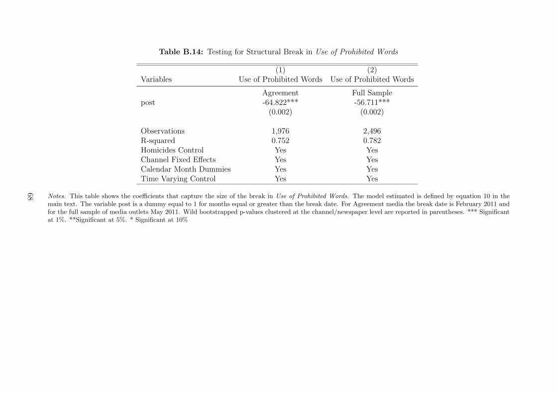
Table B.14: Testing for Structural Break in Use of Prohibited Words
(1) (2)Variables Use of Prohibited Words Use of Prohibited Words
Agreement Full Samplepost -64.822*** -56.711***
(0.002) (0.002)
Observations 1,976 2,496R-squared 0.752 0.782Homicides Control Yes YesChannel Fixed Effects Yes YesCalendar Month Dummies Yes YesTime Varying Control Yes Yes
Notes. This table shows the coefficients that capture the size of the break in Use of Prohibited Words. The model estimated is defined by equation 10 in themain text. The variable post is a dummy equal to 1 for months equal or greater than the break date. For Agreement media the break date is February 2011 andfor the full sample of media outlets May 2011. Wild bootstrapped p-values clustered at the channel/newspaper level are reported in parentheses. *** Significantat 1%. **Significant at 5%. * Significant at 10%
68

C Appendix Figures
Figure C.1: Fraction of periods in the post-policy period (t≥2011m3) in the monthlydataset
0.1
.2.3
.4F
ract
ion
of O
bser
vatio
ns in
EC
OS
EP
0 .2 .4 .6 .8 1Fraction of periods in the post-policy period
Notes. This figure shows the distribution of the fraction of periods in the post-policy period over the total
number of periods that each observation is in the monthly data. For example, 40% of the individuals in
the monthly data are only interviewed before 2011m3; while 25% are only interviewed after 2011m3.
69

Figure C.2: Testing for Structural Break in Use of Prohibited Words18
0020
0022
0024
0026
00R
esid
ual V
aria
nce
2009
m7
2010
m7
2011
m7
2012
m7
2011
m5
2011
m5
Anno
unce
men
t
Break date
Full-Sample
1800
2000
2200
2400
2600
Res
idua
l Var
ianc
e
2009
m7
2010
m7
2011
m7
2012
m7
2011
m2
2011
m2
Anno
unce
men
t
Break date
Agreement
Notes. This figure plots the sum of squared residuals as a proportion of the number of observations ofthe model defined by equation 10 in the main text. The figure at the top uses the full sample of mediaoutlets defined in section4 of the main text, while the figure at the bottom only uses Agreement mediaoutlets.
70
Top Related