


Languages
Pages
Legal


Mechanics of structuresMechanics of structures
Stresses in 2D plane, ColumnsColumns
Dr. Rajesh K. N.Assistant Professor in Civil EngineeringAssistant Professor in Civil EngineeringGovt. College of Engineering, Kannur
Dept. of CE, GCE Kannur Dr.RajeshKN
1

Module IV
Transformation of stresses and strains (two dimensional case only)
Module IV
Transformation of stresses and strains (two-dimensional case only) -equations of transformation - principal stresses - mohr's circles of stress and strain - strain rosettes - compound stresses - superposition
d it li it ti and its limitations –
Eccentrically loaded members - columns - theory of columns -buckling theory - Euler's formula - effect of end conditions -eccentric loads and secant formula
Dept. of CE, GCE Kannur Dr.RajeshKN
2

Analysis of plane stress and plane strainy p p
cosnA A θ=P
LAA
θ
PA
σ = cos
n
nAAθ
=AAn
A
22cos cos cosn
P PA Aθ θσ σ θ= = =
cosP θθ
nA A
sin sin cos sin2P Pθ θ θ σ θτ
Pθ
sinP θAn
θ
Dept. of CE, GCE Kannur Dr.RajeshKN
32n
nA Aτ = = =

2 2σ σ τ+
( ) ( )2 22cos sin cos
R n nσ σ τ
σ θ σ θ θ
= +
= +
Resultant stress on inclined plane
2 2cos cos sincos
σ θ θ θσ θ
= +=
0 2 cos sin 0nddσ σ θ θθ= ⇒ =For maximum normal stress,
0sin2 0 0σ θ θ= ⇒ =
0When 0 Pθ σ σ= = =
0 2 0ndτ θFor maximum shear stress
,maxWhen 0 , n Aθ σ σ= = =
0 0
0 cos2 0
2 90 45
n
dσ θ
θθ θ
= ⇒ =
⇒ = ⇒ =
For maximum shear stress,
Dept. of CE, GCE Kannur Dr.RajeshKN
40
,maxWhen 45 ,2 2n
PA
σθ τ= = =

nσ σ
nτσ
Rσ 2 2n nσ τ+
σ,maxnτ
σ
Dept. of CE, GCE Kannur Dr.RajeshKN
5

Element under pure shearτ
B
θ σnτ
τ
θτ
θ nσττ θ
cos sinBC AC ABσ τ θ τ θ= − −
A Cττ
. .cos . .sinsin cos cos sinsin 2
n
n
BC AC ABσ τ θ τ θσ τ θ θ τ θ θσ τ θ
= − −= − −
. . .sin . .cosn BC AC ABAC AB
τ τ θ τ θ= − +sin 2nσ τ θ= −
2 2
. .sin . .cos
cos sin
n
n
AC ABBC BC
τ τ θ τ θ
τ τ θ τ θ
= − +
= −
Dept. of CE, GCE Kannur Dr.RajeshKN
6cos2
n
nτ τ θ=
Element under biaxial normal stress
Bnτ
yσ
θ nσn
σxσθ
xσ
A C
xσ
yσsin cosBC AB ACτ σ θ σ θ= −cos sinBC AB ACσ σ θ σ θ= +
yσ
. . .sin . .cos
. .sin . .cos
n x y
n x y
BC AB ACAB ACBC BC
τ σ θ σ θ
τ σ θ σ θ
=
= −
. .cos . .sin
. .cos . .sin
n x y
n x y
BC AB ACAB ACBC BC
σ σ θ σ θ
σ σ θ σ θ
= +
= +
( )
cos sin sin cos
sin 2n x y
BC BCτ σ θ θ σ θ θ
θ
= −2 2cos sin
y
n x y
BC BCσ σ θ σ θ= +
Dept. of CE, GCE Kannur Dr.RajeshKN
7
( ) 2n x yτ σ σ= −

Element under a general two-dimensional stress
xyτxyτ
Bnττ
σ
θ θ nσ
xσ
xyτ
xσ
xyτ
xyτA C
x
xyτ
. .cos . .sin . .cos . .sinn x y xy xyBC AB AC AC ABσ σ θ σ θ τ θ τ θ= + − −
yσxy
yσ
. .cos . .sin . .cos . .sinn x y xy xyAB AC AC ABBC BC BC BC
σ σ θ σ θ τ θ τ θ= + − −
2 2cos sin sin 2n x y xyσ σ θ σ θ τ θ= + −
+
Dept. of CE, GCE Kannur Dr.RajeshKN
8cos2 sin 2
2 2x y x y
n xy
σ σ σ σσ θ τ θ
+ −= + −

i iBC AB AC AB ACθ θ θ θ. . .sin . .cos . .cos . .sin
sin cos cos sin
n x y xy xyBC AB AC AB AC
AB AC AB AC
τ σ θ σ θ τ θ τ θ
τ σ θ σ θ τ θ τ θ
= − + −
= − + −
2 2
. .sin . .cos . .cos . .sin
cos sin sin cos cos sin
n x y xy xy
n x y xy xy
BC BC BC BCτ σ θ σ θ τ θ τ θ
τ σ θ θ σ θ θ τ θ τ θ
= − + −
= − + −n x y xy xy
sin 2 cos22
x yn xy
σ στ θ τ θ
−= +
2n xy
Note: In the above derivations,
Sign convention for θ: Anticlockwise angle is +ve.g g
Sign convention for shear stress: With respect to a point inside the element, clockwise shear stress is +ve.
Dept. of CE, GCE Kannur Dr.RajeshKN
9
the element, clockwise shear stress is +ve.

σ σ σ σ+ −cos2 sin 2
2 2x y x y
n xy
σ σ σ σσ θ τ θ
+= + −
σ σ−
Th b ti i th l d t ti l ( h ) t
sin 2 cos22
x yn xy
σ στ θ τ θ= +
The above equations give the normal and tangential (shear) stresses on any plane inclined at θ with the vertical.
To find maximum/minimum value of normal stress
σ∂ ( )0nσθ
∂=
∂( )sin 2 2 cos2 0x y xyσ σ θ τ θ⇒ − − − =
2tan 2 xyτ
θ−
⇒ ( )tan 2 y
x y
θσ σ
⇒ =−
Dept. of CE, GCE Kannur Dr.RajeshKN
10

2σ σ−⎛ ⎞ sin 2 xyτθ
−=
xyτ−
( )
2
2x y
xy
σ στ⎛ ⎞
+⎜ ⎟⎝ ⎠
2θ
22
sin 2
2
y
x yxy
θσ σ
τ
=−⎛ ⎞
+⎜ ⎟⎝ ⎠
( )2
x yσ σ−
2cos2 x yσ σ
θ−
=2
222
x yxy
σ στ
−⎛ ⎞+⎜ ⎟
⎝ ⎠
cos2 sin 22 2
x y x yn xy
σ σ σ σσ θ τ θ
+ −= + −
22
max 2 2x y x y
xy
σ σ σ σσ τ
+ −⎛ ⎞⇒ = + +⎜ ⎟
⎝ ⎠⎝ ⎠
22
ix y x yσ σ σ σ
σ τ+ −⎛ ⎞
= − +⎜ ⎟
Dept. of CE, GCE Kannur Dr.RajeshKN
11
min 2 2 xyσ τ+⎜ ⎟⎝ ⎠

2222
max,min 1,3 2 2x y x y
xy
σ σ σ σσ σ τ
+ −⎛ ⎞= = ± +⎜ ⎟
⎝ ⎠ ( )2
tan 2 xy
x y
τθ
σ σ−
=−
22
max,min 1,3 2 2x y x y
xy
σ σ σ σσ σ τ
+ −⎛ ⎞= = ± +⎜ ⎟
⎝ ⎠ ( )2
tan 2 xy
x y
τθ
σ σ−
=−
Principal stresses Principal planes
σ σ−
Maximum shear stress
We know, sin 2 cos22
x yn xy
σ στ θ τ θ= +
F i h t 0nτ∂For maximum shear stress, 0n
θ=
∂
( )cos2 2 sin 2 0x y xyσ σ θ τ θ⇒ − − =( )x y xy
( )tan 2 x yσ σ
θ−
⇒ =
Dept. of CE, GCE Kannur Dr.RajeshKN
12
tan 22 xy
θτ
⇒
2
( )2
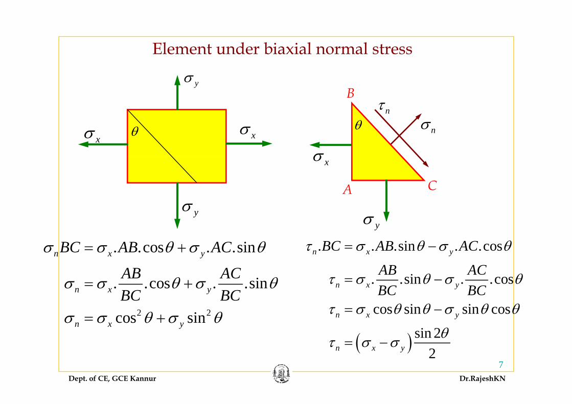
For max normal stress, tan 2 xyn
x y
τθ
σ σ−
=−
( )For max shear stress, tan 2
2x y
s
σ σθ
τ−
= 1tan 2θ−
=2 xyτ tan 2 nθ
( )0cot 2 tan 2 90n nθ θ= − = ±( )n n
02 2 90s nθ θ= ±s n
045s nθ θ= ±
Hence, planes of maximum shear stress are at 450 to the principal planes
Dept. of CE, GCE Kannur Dr.RajeshKN
13
p

To get maximum shear stress
( )2
2
2x y
xy
σ στ
−⎛ ⎞+⎜ ⎟
⎝ ⎠
22
cos2 xys
x y
τθ
σ στ
=−⎛ ⎞
+⎜ ⎟
g
τ
( )2
x yσ σ− 2 y⎜ ⎟⎝ ⎠
2 sθ2
yxyτ+⎜ ⎟
⎝ ⎠
sin 2 x yσ σθ
−=xyτ
22
sin 2
22
s
x yxy
θσ σ
τ
=−⎛ ⎞
+⎜ ⎟⎝ ⎠
,max 2 22 2
22
x y x y xyn xy
x y x y
σ σ σ σ ττ τ
σ σ σ στ τ
− −= +
− −⎛ ⎞ ⎛ ⎞+ +⎜ ⎟ ⎜ ⎟
2σ σ−⎛ ⎞
22 2xy xyτ τ+ +⎜ ⎟ ⎜ ⎟
⎝ ⎠ ⎝ ⎠
2σ σ⎛ ⎞2,max 2
x yn xy
σ στ τ⎛ ⎞
= +⎜ ⎟⎝ ⎠
2,max,min 2
x yn xy
σ στ τ
−⎛ ⎞= ± +⎜ ⎟
⎝ ⎠
Dept. of CE, GCE Kannur Dr.RajeshKN
14

2⎛ ⎞ 2
1,3 2
We kno2
w, x y x yxy
σ σ σ σσ τ
+ −⎛ ⎞= ± +⎜ ⎟
⎝ ⎠
22
1 3 ,max2 22
x yxy n
σ σσ σ τ τ
−⎛ ⎞− = + =⎜ ⎟
⎝ ⎠
1 3,max 2n
σ στ −=
2
To get normal stress on planes of maximum shear stress
2 22 2
2 2x y x y xy x y
n xy
x y x y
σ σ σ σ τ σ σσ τ
σ σ σ σ
+ − −= + −
− −⎛ ⎞ ⎛ ⎞2 222 2
x y x yxy xy
σ σ σ στ τ⎛ ⎞ ⎛ ⎞
+ +⎜ ⎟ ⎜ ⎟⎝ ⎠ ⎝ ⎠
x yσ σ+ th l f h t
Dept. of CE, GCE Kannur Dr.RajeshKN
152x y
nσ = , on the planes of max shear stressaverageσ=

Problem: Find the principal stresses (including principal planes) and maximum shear stress (including its plane)
260 N
280 N mmPrincipal stresses
2120 N mm
260 N mm
2120 N mm2
2max,min 1,3 2 2
x y x yxy
σ σ σ σσ σ τ
+ −⎛ ⎞= = ± +⎜ ⎟
⎝ ⎠
Principal stresses
280 N mm
260 N mm
⎝ ⎠
22
max min 1 3120 80 120 80 60σ σ − − − +⎛ ⎞= = ± +⎜ ⎟
⎝ ⎠max,min 1,3 60
2 2σ σ ± +⎜ ⎟
⎝ ⎠
100 63 24σ σ= = − ±max,min 1,3 100 63.24σ σ= = ±
2max 1 163.24 N mmσ σ∴ = = −max 1
2min 3and 36.75 N mmσ σ= = −
Dept. of CE, GCE Kannur Dr.RajeshKN
16

2tan 2 xyτ
θ−
=Principal planes 2 60− ×= 3=( )tan 2
x y
θσ σ
=−
Principal planes( )120 80
=− +
3=
( )12 tan 3 71 57θ −= = 35 78θ∴ =( )2 tan 3 71.57θ = = 35.78θ∴ =
1 35.78θ∴ =1
3 35.78 90 125.78θ = + =
xyτxyτ
35 78
xσxyτ 3σ1σ
35.78
yσxyτ
Dept. of CE, GCE Kannur Dr.RajeshKN
17

Maximum shear stress
1 3,max 2n
σ στ −=
Maximum shear stress
163.25 36.752
− += 263.25 N mm= −
2 2
Planes of maximum shear stress
( )tan 2 x yσ σ
θ−
=120 80− +
=tan 22s
xy
θτ
=2 60
=×
xyτxyτ 1 120 802 tθ − − +⎛ ⎞
⎜ ⎟
18.43= −σ
xy
9.22
12 tan2 60
θ ⎛ ⎞= ⎜ ⎟×⎝ ⎠
18.43xσ
xyτ
xyτ ,maxnτ
9.22θ = −
Dept. of CE, GCE Kannur Dr.RajeshKN
18yσ
xy

cos2 sin 2x y x yσ σ σ σσ θ τ θ
+ −= +
Mohr’s circle
cos2 sin 22 2n xyσ θ τ θ= + −
cos2 sin 2x y x yσ σ σ σσ θ τ θ
+ −= i
sin 2 cos22
x yn xy
σ στ θ τ θ
−= +
cos2 sin 22 2n xyσ θ τ θ− = − i
ii2n xy
Squaring and adding the above equations,
( ) ( )2 2
22
2 2x y x y
n n xy
σ σ σ σσ τ τ
+ −⎛ ⎞ ⎛ ⎞− + = +⎜ ⎟ ⎜ ⎟
⎝ ⎠ ⎝ ⎠2 2⎝ ⎠ ⎝ ⎠
( ) ( )2 2 20n av n Rσ σ τ− + − =
This is equation of a circle with centre and radius ( )2
2
2x y
xy
σ στ
−⎛ ⎞+⎜ ⎟
⎝ ⎠( ),0avσ
Dept. of CE, GCE Kannur Dr.RajeshKN
19Let us draw this circle!

Mohr’s circlexyτ
( ),y xyσ τxσxyτ
xyxyτ
22
2y x
xy
σ στ
−⎛ ⎞+⎜ ⎟
⎝ ⎠yσ
xyτ
σy
τxyτ
2y xσ σ+
yσx σσ3 σ1α
2y xσ σ−
τxy
( ),x xyσ τ− 1 2tan 2xy
y x
τα θ
σ σ− −
= =−
Dept. of CE, GCE Kannur Dr.RajeshKN
20: Principal stresses σ1, σ3measured clockwise α

Mohr’s circlexyτ
xσxyτ
y
xyτ
( ),x xyσ τ
yσxyτ
τ
22
2y x
xy
σ στ
−⎛ ⎞+⎜ ⎟
⎝ ⎠
σyσx
τxyτ
σ3α
x
σ3
σ1
2y xσ σ+
2y xσ σ−
τxy
2
1 2tan 2xy
y x
τα θ
σ σ−= =
−( ),y xyσ τ−
Dept. of CE, GCE Kannur Dr.RajeshKN
21
y
measured anticlockwise α

•Mohr’s circle is a graphical representation of the state of stress in an •Mohr s circle is a graphical representation of the state of stress in an element.
E i h i l h l d h •Every point on the circle represents the normal and shear stress on a plane.
•While x-coordinate of a point on the circle represents the normal stress on a plane, y-coordinate represents the shear stress on that plane.
•Procedure for construction of Mohr’s circle
Dept. of CE, GCE Kannur Dr.RajeshKN
22

Maximum shear stress from Mohr’s circlexyτ
( ),y xyσ τxσxyτ
xyxyτ
Max shear 2
2
2y x
xy
σ στ
−⎛ ⎞+⎜ ⎟
⎝ ⎠ yσxyτ
Max shear stress
1 3max 2n
σ στ −=
σy
τxyτ ,max 2n
yσx σσ3 σ12θ
τxy
( ),x xyσ τ−
Dept. of CE, GCE Kannur Dr.RajeshKN
23

Principal planes from Mohr’s circle
xyτ( ),y xyσ τxy
xyτθ
στxyτ
σ
σyσx
τxy
σσ3 σ1
( )
2θ3σ1σ
xσxyτ( ),x xyσ τ−
σ
yσxyτ
3σ1σ
3σ
Dept. of CE, GCE Kannur Dr.RajeshKN
24
3
1σ
260 N
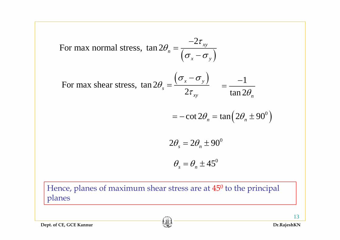
280 N mmProblem: Find principal stresses, principal
2120 N mm
260 N mm
2120 N mm
planes and max shear stress analytically. Draw Mohr’s circle and verify graphically.
280 N mm
260 N mm
( )( )120,60−
τ60 18.442
71 56θ
80120
60
σ σ3σ1
3σ1σ
35.7871.56=
τ
9.22
60 1,maxnτ
Dept. of CE, GCE Kannur Dr.RajeshKN25
( )80, 60− −

Problems: Find principal stresses, principal planes and max shear stress analytically. Draw Mohr’s circle and verify graphically.analytically. Draw Mohr s circle and verify graphically.
151080
5015
1515
5050
10
1010
5050
3015
30
15
80
1010
15
50
5
2020
20
50
5
5020
Dept. of CE, GCE Kannur Dr.RajeshKN
26

Transformation of strains
σ σ σ σ+ − sin 2 cos2x yσ στ θ τ θ
−+cos2 sin 2
2 2x y x y
n xy
σ σ σ σσ θ τ θ
+= + − sin 2 cos2
2y
n xyτ θ τ θ= +
The above equations, which give the normal and tangential (shear) stresses on any plane inclined at θ with the vertical, are called stress transformation equations.equations.
Similarly strain transformation equations can be derived as follows:
2 2cos sin sin cosn x y xyε ε θ ε θ γ θ θ= + −
cos2 sin 22 2 2
x y x y xyn
ε ε ε ε γε θ θ
+ −= + −OR,
Dept. of CE, GCE Kannur Dr.RajeshKN27
sin 2 cos22 2 2
x y xyn ε ε γγ θ θ−
= +and,

Principal strains:Planes on which
i i l t i tPrincipal strains: principal strains act:2 2
max min 1 3x y x y xyε ε ε ε γ
ε ε+ −⎛ ⎞ ⎛ ⎞
= = ± +⎜ ⎟ ⎜ ⎟⎝ ⎠ ⎝ ⎠ ( )tan 2 xyγ
β−
=max,min 1,3 2 2 2⎜ ⎟ ⎜ ⎟
⎝ ⎠ ⎝ ⎠ ( )x yε ε−
Strain Rosettes
M t f l t i i i l• Measurement of normal strains is simple.
• Strain gages are placed as a cluster, along several gage lines through a pointa point
• This arrangement of strain gages is called a strain rosette
• If three measurements are taken at a rosette (in three directions), the information is sufficient to get the complete state of plane strain at a point
Dept. of CE, GCE Kannur Dr.RajeshKN
p

03 90θ =
1 2 3, ,θ θ θε ε ε are measured from strain gages0
2 45θ =
1 2 3, ,θ θ θε ε ε are measured from strain gages
0 45 90ε ε ε45 degree rosette:
1 0θ =
0 45 90, ,ε ε ε45 degree rosette:
0 60 120, ,ε ε ε60 degree rosette:
Rectangular strain rosetteFrom strain transformation equations,
g(45 degree rosette)2 2cos sin sin cosn x y xyε ε θ ε θ γ θ θ= + −
Hence, for a 45 degree rosette, 0 0 0x xε ε ε= + − =
45 0.5 0.5 0.5x y xyε ε ε γ= + −y y
90 0 0y yε ε ε= + − =
Dept. of CE, GCE Kannur Dr.RajeshKN
From the above, we can get , ,x y xyε ε γ

Problem: Using a 60 degree rosette, the following strains are obtained at i t D t i t i t d i i l t ia point. Determine strain components and principal strains.
0 60 12040 , 980 , 330ε μ ε μ ε μ= = =
, ,x y xyε ε γ
We have, 2 2cos sin sin cosn x y xyε ε θ ε θ γ θ θ= + −
2 20 cos 0 sin 0 sin cos0x y xyε ε ε γ θ∴ = + −
i.e., 40 0 0 40x xε ε= + − ⇒ =
0 x y xyγ
60 980 0.25 0.75 0.433x y xyε ε ε γ⇒ = + −
120 330 0.25 0.75 0.433x y xyε ε ε γ⇒ = + +
40 , 860 , 750x y xyε μ ε μ γ μ= = = −
y y
From the above, we can get
Principal strains and their planes can be obtained from:
2 2ε ε ε ε γ+ −⎛ ⎞ ⎛ ⎞ tan 2 xyγβ
−=
Dept. of CE, GCE Kannur Dr.RajeshKN
max,min 1,3 2 2 2x y x y xyε ε ε ε γ
ε ε+ ⎛ ⎞ ⎛ ⎞
= = ± +⎜ ⎟ ⎜ ⎟⎝ ⎠ ⎝ ⎠ ( )tan 2
x y
βε ε
=−

Theory of columnsyCompression member: A structural member loaded in compression
Column: A vertical compression member
Strut: An inclined compression member – as in roof trusses
Stanchion: A compression member made of rolled steel section
Classification of columns based on mode of failure
Short columns: Failure by crushing under axial compressionL ( l d ) l F il b l l b di
Intermediate (medium length) columns: Failure by
Long (slender) columns: Failure by lateral bending (buckling)
Dept. of CE, GCE Kannur Dr.RajeshKN
31
Intermediate (medium length) columns: Failure by combination of buckling and crushing

Equilibrium: qu b u : Stable, neutral, unstable
Dept. of CE, GCE Kannur Dr.RajeshKN
32
L d th t b i d b th b b f f il
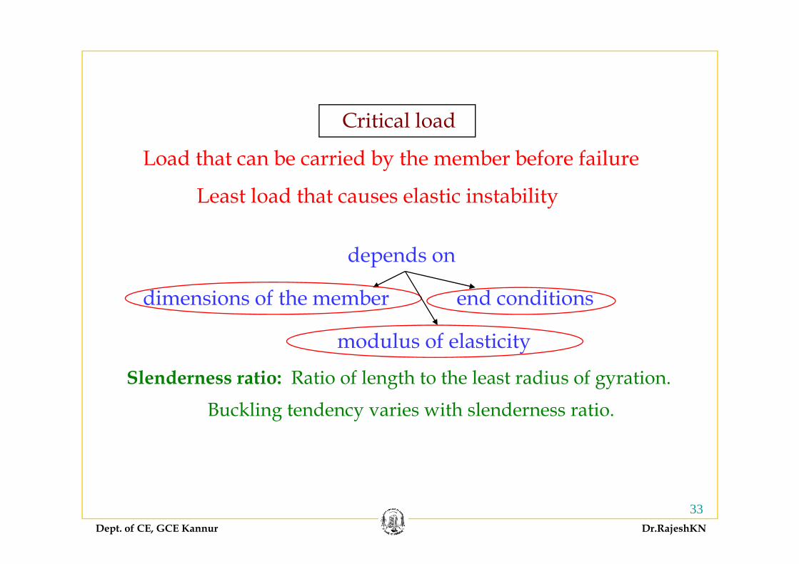
Critical load
Load that can be carried by the member before failure
Least load that causes elastic instability
depends on
dimensions of the member end conditions
modulus of elasticity
Slenderness ratio: Ratio of length to the least radius of gyration.
Buckling tendency varies with slenderness ratio
modulus of elasticity
Buckling tendency varies with slenderness ratio.
Dept. of CE, GCE Kannur Dr.RajeshKN
33

Euler’s theory – Leonhard Euler (1757)y ( )
2d y
Both ends hinged PEI MR
=2d yEI P
2d y2
d yEI Mdx
⇒ = A2
yEI Pydx
⇒ = −2 0d yEI Py
dx+ =
2
2 0d y P y+ =2 ydx EI
P P⎛ ⎞ ⎛ ⎞Solution for the above differential equation is:
yXX
l1 2cos sinP Py C x C xEI EI
⎛ ⎞ ⎛ ⎞= +⎜ ⎟ ⎜ ⎟
⎝ ⎠ ⎝ ⎠When 0, 0x y= = 1 0C⇒ =
B
xWhen 0, 0x y 1
When , 0x l y= = 20 sin PC lEI
⎛ ⎞⇒ = ⎜ ⎟
⎝ ⎠
P
B⎝ ⎠
sin 0 0, ,2 ,3 ,4 ...P Pl lEI EI
π π π π⎛ ⎞
= ⇒ =⎜ ⎟⎝ ⎠
Dept. of CE, GCE Kannur Dr.RajeshKN
34
P, where 0,1,2,3,4...Pl n n
EIπ= =

2 2
2
n EIPlπ
=
2 sin Py C xEI
⎛ ⎞= ⎜ ⎟
⎝ ⎠
2 sin n xCLπ⎛ ⎞= ⎜ ⎟
⎝ ⎠
The least practical
2EIP π
The least practical value for P is:
Critical load2crEIP
lπ
=
sin xy C π⎛ ⎞= ⎜ ⎟The corresponding mode shape is:
Dept. of CE, GCE Kannur Dr.RajeshKN
35
2 siny CL
= ⎜ ⎟⎝ ⎠
The corresponding mode shape is:

Assumptions in Euler’s theoryAssumptions in Euler s theory
• Material is homogeneous and isotropic • Axis of column is perfectly straight when unloaded• Line of thrust coincides exactly with the unstrained axis of the column• Column fails by buckling alone• Flexural rigidity EI is uniform
S lf h f l l d • Self weight of column is neglected • Stresses are within elastic limit
Dept. of CE, GCE Kannur Dr.RajeshKN
36

Euler’s theoryP
y
2d yEI M
One end fixed and the other end free
( )2d yEI P yδ⇒ = −
P
Aδ
2
yEI Mdx
= ( )2EI P ydx
δ⇒ =
2d yEI P Pδ2d y P Py δ
+ = y2
yEI Py Pdx
δ+ = 2 ydx EI EI
+ = y
lSolution for the above differential equation is:
1 2cos sinP Py C x C xEI EI
δ⎛ ⎞ ⎛ ⎞
= + +⎜ ⎟ ⎜ ⎟⎝ ⎠ ⎝ ⎠ xEI EI⎝ ⎠ ⎝ ⎠
When 0, 0x y= = 1C δ⇒ = −
x
B
Dept. of CE, GCE Kannur Dr.RajeshKN
37

dy P P P P⎛ ⎞ ⎛ ⎞
dy P
1 2sin cosdy P P P PC x C xdx EI EI EI EI
⎛ ⎞ ⎛ ⎞= − +⎜ ⎟ ⎜ ⎟
⎝ ⎠ ⎝ ⎠
When 0, 0dyxdx
= =2 20 0 0PC C
EI⇒ = = ⇒ =
When x l y δ= = cos Plδ δ δ⎛ ⎞
⇒ +⎜ ⎟
3 5cos 0P Pl l π π π⎛ ⎞⇒⎜ ⎟
When ,x l y δ= = cos lEI
δ δ δ⇒ = − +⎜ ⎟⎝ ⎠
cos 0 , , ...2 2 2
l lEI EI
= ⇒ =⎜ ⎟⎝ ⎠
Pl πTh l t ti l l i2
PlEI
π=
2EIP π 2EIP π
The least practical value is:
2el l= Effective length24EIPl
π= 2
e
EIPl
π=
P⎛ ⎞ ⎛ ⎞
e Effective length
Dept. of CE, GCE Kannur Dr.RajeshKN
38cos 1 cos
2 e
P xy xEI l
πδ δ δ⎛ ⎞ ⎛ ⎞
= − + = −⎜ ⎟ ⎜ ⎟⎝ ⎠⎝ ⎠
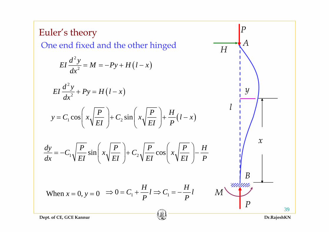
Euler’s theory Py
( )2d yEI M P H l
One end fixed and the other hinged HA
( )2
yEI M Py H l xdx
= = − + −
( )2d yEI P H l y( )2
yEI Py H l xdx
+ = −
( )cos sinP P HC C l⎛ ⎞ ⎛ ⎞
+ +⎜ ⎟ ⎜ ⎟
y
l( )1 2cos siny C x C x l x
EI EI P= + + −⎜ ⎟ ⎜ ⎟
⎝ ⎠ ⎝ ⎠
x⎛ ⎞ ⎛ ⎞
x1 2sin cosdy P P P P HC x C x
dx EI EI EI EI P⎛ ⎞ ⎛ ⎞
= − + −⎜ ⎟ ⎜ ⎟⎝ ⎠ ⎝ ⎠
When 0 0x y= = 1 10 H HC l C l⇒ = + ⇒ = −
B
M
Dept. of CE, GCE Kannur Dr.RajeshKN
39
When 0, 0x y 1 1P PP
M
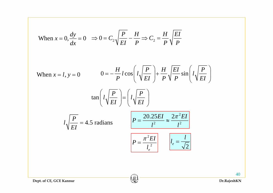
When 0, 0dyxdx
= = 2 20 P H H EIC CEI P P P
⇒ = − ⇒ =
When 0x l y= = 0 cos sinH P H EI Pl l l⎛ ⎞ ⎛ ⎞
= − +⎜ ⎟ ⎜ ⎟
tan P Pl l⎛ ⎞ ⎛ ⎞⎜ ⎟ ⎜ ⎟
When , 0x l y= = 0 cos sinl l lP EI P P EI
+⎜ ⎟ ⎜ ⎟⎝ ⎠ ⎝ ⎠
tan l lEI EI
=⎜ ⎟ ⎜ ⎟⎝ ⎠ ⎝ ⎠
P220.25 2EI EIP π
4.5 radiansPlEI
= 2 2Pl l
= ≈
2EIP π ll2
e
EIPl
π=
2el =
Dept. of CE, GCE Kannur Dr.RajeshKN
40

Euler’s theory Py
2d yEI M M P
Both ends fixed A M0
02
yEI M M Pydx
= = −
2d yEI P M y20d y P M
02
yEI Py Mdx
+ =
0P P M⎛ ⎞ ⎛ ⎞
y
l
02
y ydx EI EI
+ =
01 2cos sinP P My C x C x
EI EI P⎛ ⎞ ⎛ ⎞
= + +⎜ ⎟ ⎜ ⎟⎝ ⎠ ⎝ ⎠
⎛ ⎞ ⎛ ⎞x
1 2sin cosdy P P P PC x C xdx EI EI EI EI
⎛ ⎞ ⎛ ⎞= − +⎜ ⎟ ⎜ ⎟
⎝ ⎠ ⎝ ⎠
x
When 0 0x y= = 0 01 10 M MC C⇒ = + ⇒ = −
B
M
Dept. of CE, GCE Kannur Dr.RajeshKN
41
When 0, 0x y 1 1P P PM0

When 0, 0dyxdx
= = 2 20 0PC CEI
⇒ = ⇒ =
When 0x l y= =0 00 cosM P Ml
P EI P⎛ ⎞
= − +⎜ ⎟ 0 1 cos 0M Pl⎡ ⎤⎛ ⎞
⇒ − =⎢ ⎥⎜ ⎟
cos 1Pl⎛ ⎞⎜ ⎟
When , 0x l y= = P EI P⎜ ⎟⎝ ⎠ P EI⎢ ⎥⎜ ⎟
⎢ ⎥⎝ ⎠⎣ ⎦
0 2 4 6Pl π π π⇒ =cos 1lEI
=⎜ ⎟⎝ ⎠
24 EIP π
0,2 ,4 ,6 ...lEI
π π π⇒ =
2Pl π2P
l=
2EI l
2lEI
π=
2
2e
EIPl
π= 2e
ll =
Dept. of CE, GCE Kannur Dr.RajeshKN
42

Effective lengthEnd conditions
Both ends hinged
g
l
One end fixed and the other end free 2l
B th d fi d
One end fixed and the other hinged 2l
Both ends fixed 2l
Dept. of CE, GCE Kannur Dr.RajeshKN
43

Limitations of Euler’s theoryLimitations of Euler s theory
• Applicable to ideal cases only. There may be imperfections in the l th l d t tl th h th t id f th
2
column, the load may not pass exactly through the centroid of the column section• Direct stress is not taken into account
2
2Ee
EIPl
π=• Strength of the material is not taken into account
2
2E
Ee
P EIA Al
πσ = =
2 2 2EAr Eπ π22E
e e
EAr EAl l
r
π πσ⇒ = =⎛ ⎞⎜ ⎟⎝ ⎠
Dept. of CE, GCE Kannur Dr.RajeshKN
44

σ Eσ E
l /
Validity limits of Euler’s formula
le /r
Dept. of CE, GCE Kannur Dr.RajeshKN
45Critical stress for mild steel with E=2x10⁵ MPa
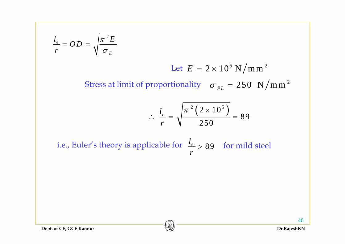
2l Eπe
E
l EODr
πσ
= =
5 22 10 NEL t2250 N m mPLσ =Stress at limit of proportionality
5 22 10 N m mE = ×Let
( )2 52 1089
250elr
π ×∴ = =
250r
i.e., Euler’s theory is applicable for 89el > for mild steelr
Dept. of CE, GCE Kannur Dr.RajeshKN
46

Rankine’s theoryy
2
2EulerEIP π
=
c cP Aσ=For short compression members,
For long columns,2Euler
elg ,
Rankine proposed a general empirical formula:
1 1 1
Rankine c EulerP P P= + For a short compression member, PE is very large.
P P∴ ≈Rankine cP P∴ ≈
For long columns, 1/PEuler is very large.2
2
1 elP EIπ
=
Rankine EulerP P≈
EulerP EIπ
21 1 1
R ki EIP A πσ= + 2I Ar=
Dept. of CE, GCE Kannur Dr.RajeshKN
472
Rankine c
e
EIP Al
πσ

1 1 1
22 rEπ σ
⎛ ⎞+⎜ ⎟
22
1 1 1
Rankine cP A rEAl
σπ
= +⎛ ⎞⎜ ⎟⎝ ⎠
22
ce
Rankinec
ElA
P rEl
π σ
σ π
+⎜ ⎟⎝ ⎠=
⎛ ⎞⎜ ⎟⎝ ⎠
2 2c c
RankineA AP
l lσ σσ
= =⎛ ⎞ ⎛ ⎞
ca σ=
el⎝ ⎠ cel
⎜ ⎟⎝ ⎠
21 1c e el laE r r
σπ
⎛ ⎞ ⎛ ⎞+ +⎜ ⎟ ⎜ ⎟⎝ ⎠ ⎝ ⎠
2aEπ
2 2Crushing loadc
RankineAPl l
σ= =
⎛ ⎞ ⎛ ⎞
2
1 elar
⎛ ⎞+ ⎜ ⎟⎝ ⎠1 1e el la a
r r⎛ ⎞ ⎛ ⎞+ +⎜ ⎟ ⎜ ⎟⎝ ⎠ ⎝ ⎠
r⎝ ⎠
Factor that accounts for bucklingg
Dept. of CE, GCE Kannur Dr.RajeshKN
48

Find the length of the column for which Rankine’s and Euler’s formulae give the same buckling load:
Rankine EulerP P=
2A EIσ π 1/22 2⎛ ⎞2 2
1
c
ee
A EIlla
r
σ π=
⎛ ⎞+ ⎜ ⎟⎝ ⎠
1/22 2
2ec
ErlEa
πσ π⎛ ⎞
= ⎜ ⎟−⎝ ⎠
Dept. of CE, GCE Kannur Dr.RajeshKN
49

Problem: Compare the buckling (crippling) loads given by Rankine’s Problem: Compare the buckling (crippling) loads given by Rankine s and Euler’s formulae for a tubular strut hinged at both ends, 6 m long having outer diameter 15 cm and thickness 2 cm. Given,
4 2 2 18 10 N mm , 567 N mm ,1600cE aσ= × = =
For what length of the column does the Euler’s formula cease to apply?For what length of the column does the Euler s formula cease to apply?2
2EulerEIP
lπ
=
( )4 4 4150 110 17663604.69 mm64
I π= − =
el
6 m 6000 mmel l= = =( )64 e
2
2 387406.2 NEulerEIP
lπ
= = 387.4 kN=2Euler
el
( )2 2 2π
Dept. of CE, GCE Kannur Dr.RajeshKN
50
( )2 2 2150 110 8168.141 mm4
A π= − =

c AP σ2
1
cRankine
e
Plar
σ=
⎛ ⎞+ ⎜ ⎟⎝ ⎠
2 417663604.69 mmI Ar= = 17663604.69 46.503 mm8168.141
IrA
= = =
567 8168.141 406097 78 NP × 406 098 kN=2 406097.78 N1 60001
1600 46.503
RankineP = =⎛ ⎞+ ⎜ ⎟⎝ ⎠
406.098 kN=
2
2EEπσ = ( )2 48 10
37 317el π ×∴ = =
2EP EIπσ = =
To find the length of the column above which Euler’s formula is applicable
2Eelr
σ⎛ ⎞⎜ ⎟⎝ ⎠
37.317567r
∴ = =2E
eA Alσ = =
46 503 37 317l 1735 34 m m 1 735 m
Dept. of CE, GCE Kannur Dr.RajeshKN
51
46.503 37.317el∴ = × 1735.34 m m 1.735 m= =
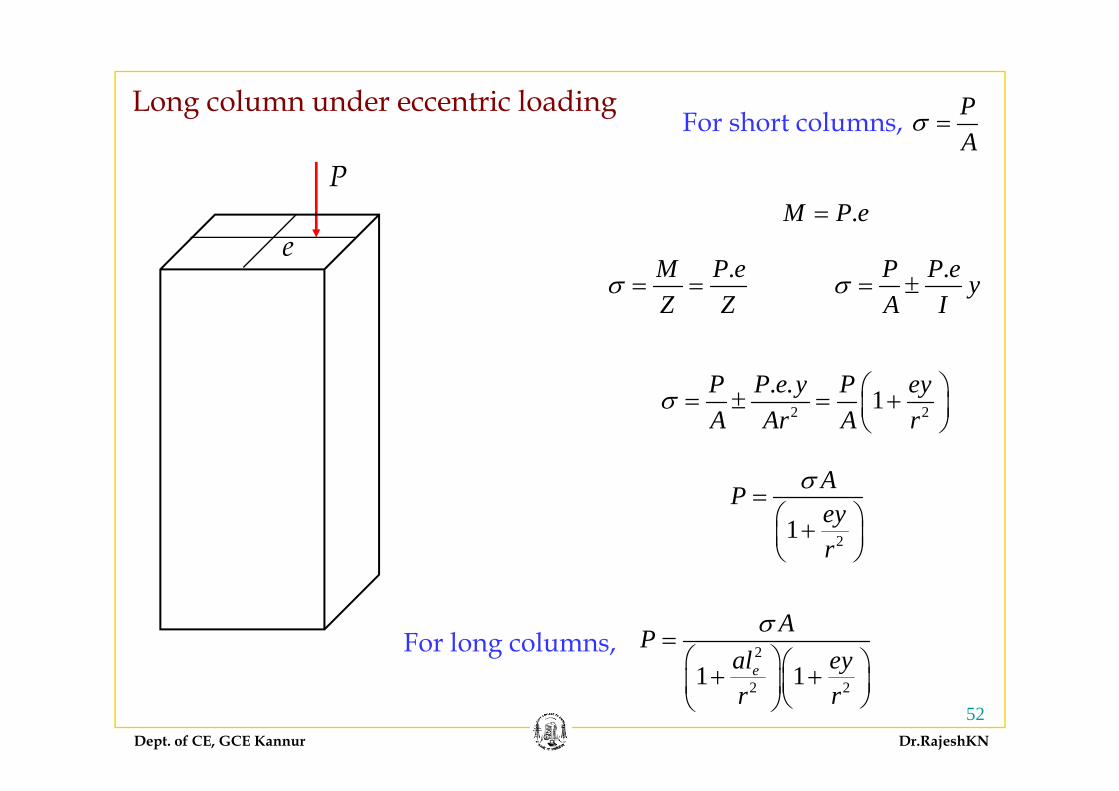
Long column under eccentric loading Pσ =For short columns
PA
σ =
M P e=
For short columns,
e.M P e
Z Zσ = =
.M P e=
.P P e yA I
σ = ±Z Z A I
. . 1P P e y P ey⎛ ⎞± +⎜ ⎟2 21y yA Ar A r
σ ⎛ ⎞= ± = +⎜ ⎟⎝ ⎠
Aσ
21
APeyr
σ=⎛ ⎞+⎜ ⎟⎝ ⎠
2
APal eyσ
=⎛ ⎞⎛ ⎞
For long columns,
Dept. of CE, GCE Kannur Dr.RajeshKN
522 21 1eal ey
r r⎛ ⎞⎛ ⎞+ +⎜ ⎟⎜ ⎟⎝ ⎠⎝ ⎠
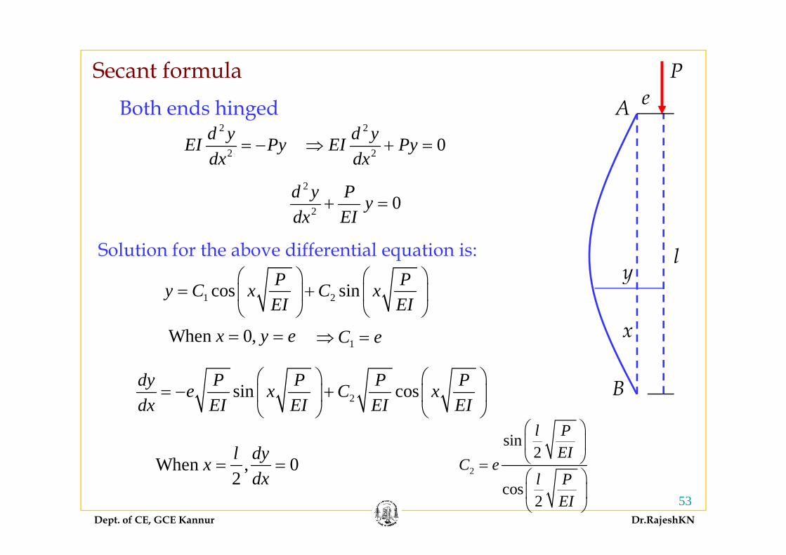
Secant formula P
A e2
2 0d yEI Py⇒ + =2
2
d yEI Py= −
Both ends hinged
2 ydx
2
2 0d y P yd EI
+ =
2 ydx
yl
2dx EI
P P⎛ ⎞ ⎛ ⎞Solution for the above differential equation is:
y
x
1 2cos sinP Py C x C xEI EI
⎛ ⎞ ⎛ ⎞= +⎜ ⎟ ⎜ ⎟
⎝ ⎠ ⎝ ⎠When 0,x y e= = 1C e⇒ =
B
When 0,x y e 1C e⇒
2sin cosdy P P P Pe x C xdx EI EI EI EI
⎛ ⎞ ⎛ ⎞= − +⎜ ⎟ ⎜ ⎟
⎝ ⎠ ⎝ ⎠dx EI EI EI EI⎝ ⎠ ⎝ ⎠
When 0l dyx = =sin
2l P
EIC e
⎛ ⎞⎜ ⎟⎝ ⎠=
Dept. of CE, GCE Kannur Dr.RajeshKN
53
When , 02
xdx
= = 2
cos2
C el P
EI
=⎛ ⎞⎜ ⎟⎝ ⎠

l P⎡ ⎤⎛ ⎞sin
2cos sin
cos
l PEIP Py e x x
EI EIl P
⎡ ⎤⎛ ⎞⎢ ⎥⎜ ⎟⎛ ⎞ ⎛ ⎞⎝ ⎠⎢ ⎥= +⎜ ⎟ ⎜ ⎟⎢ ⎥⎛ ⎞⎝ ⎠ ⎝ ⎠⎢ ⎥⎜ ⎟
2sin2l P
EI⎡ ⎤⎛ ⎞⎢ ⎥⎜ ⎟⎛ ⎞
cos2 EI
⎢ ⎥⎜ ⎟⎢ ⎥⎝ ⎠⎣ ⎦
l P⎛ ⎞max
2When , cos
2 2cos
2
EIl l Px y y eEI l P
EI
⎢ ⎥⎜ ⎟⎛ ⎞ ⎝ ⎠⎢ ⎥= = = +⎜ ⎟⎢ ⎥⎛ ⎞⎝ ⎠⎢ ⎥⎜ ⎟⎢ ⎥⎝ ⎠⎣ ⎦
max .sec2l Py e
EI⎛ ⎞
⇒ = ⎜ ⎟⎝ ⎠
max max . .sec2l PM Py P e
EI⎛ ⎞
= = ⎜ ⎟⎝ ⎠2 EI⎝ ⎠
P My P Pey l P P ey l P⎡ ⎤⎛ ⎞ ⎛ ⎞max 2sec 1 sec
2 2c c cP My P Pey l P P ey l P
A I A I EI A r EIσ
⎡ ⎤⎛ ⎞ ⎛ ⎞= + = + = +⎢ ⎥⎜ ⎟ ⎜ ⎟
⎢ ⎥⎝ ⎠ ⎝ ⎠⎣ ⎦
Dept. of CE, GCE Kannur Dr.RajeshKN
54

Secant formula Pδ
One end fixed and the other end free Aδ e
( )2
2
d yEI P e yδ= + −
( )2
2
d y P Py ed EI EI
δ+ = +y
( )2 ydx
( )2dx EI EI
P P⎛ ⎞ ⎛ ⎞Solution for the above differential equation is:
l
( )1 2cos sinP Py C x C x eEI EI
δ⎛ ⎞ ⎛ ⎞
= + + +⎜ ⎟ ⎜ ⎟⎝ ⎠ ⎝ ⎠
When 0, 0x y= = ( )1C eδ⇒ = − +
xWhen 0, 0x y ( )1
( ) 2sin cosdy P P P Pe x C xdx EI EI EI EI
δ⎛ ⎞ ⎛ ⎞
= − + +⎜ ⎟ ⎜ ⎟⎝ ⎠ ⎝ ⎠
Bdx EI EI EI EI⎝ ⎠ ⎝ ⎠
When 0 0dyx = = 0C⇒ =
Dept. of CE, GCE Kannur Dr.RajeshKN
55
When 0, 0xdx
= = 2 0C⇒ =

When x l y δ= = ( ) ( )cos Pe l eδ δ δ⎛ ⎞
⇒ = + + +⎜ ⎟When ,x l y δ= = ( ) ( )cose l eEI
δ δ δ⇒ = − + + +⎜ ⎟⎝ ⎠
( ) 1 Plδ δ⎡ ⎤⎛ ⎞
⇒ + ⎢ ⎥⎜ ⎟( ) 1 cose lEI
δ δ⇒ = + −⎢ ⎥⎜ ⎟⎢ ⎥⎝ ⎠⎣ ⎦
( )cos Pe l eδ⎛ ⎞
⇒ + ⎜ ⎟( )cose l eEI
δ⇒ + =⎜ ⎟⎝ ⎠
( ) sec Pe e lδ⎛ ⎞
⇒ + = ⎜ ⎟
( ) PM P P lδ⎛ ⎞
+ ⎜ ⎟
( ) .sece e lEI
δ⇒ + = ⎜ ⎟⎝ ⎠
( )max . .secM P e P e lEI
δ= + = ⎜ ⎟⎝ ⎠
⎡ ⎤⎛ ⎞ ⎛ ⎞max 2sec 1 secc c cP My P Pey P P ey Pl l
A I A I EI A r EIσ
⎡ ⎤⎛ ⎞ ⎛ ⎞= + = + = +⎢ ⎥⎜ ⎟ ⎜ ⎟
⎢ ⎥⎝ ⎠ ⎝ ⎠⎣ ⎦
Dept. of CE, GCE Kannur Dr.RajeshKN
56

max . .sec2el PM P e
EI⎛ ⎞
= ⎜ ⎟⎝ ⎠
In general,
2 EI⎝ ⎠
max 21 sec2
c eP ey l PA r EI
σ⎡ ⎤⎛ ⎞
= +⎢ ⎥⎜ ⎟⎢ ⎥⎝ ⎠⎣ ⎦2A r EI⎢ ⎥⎝ ⎠⎣ ⎦
For short compression members (no buckling), max .M P e=
For long columns (with buckling) el PM P⎛ ⎞⎜ ⎟For long columns (with buckling),
max . .sec2eM P e
EI= ⎜ ⎟
⎝ ⎠
Dept. of CE, GCE Kannur Dr.RajeshKN
57

Problem: A hollow mild steel column with internal diameter 80 mmand external diameter 100 mm is 2.4 m long, hinged at both ends,carries a load of 60 kN at an eccentricity of 16mm from the geometricalaxis. Calculate the maximum and minimum stresses in the column.Also find the maximum eccentricity so that no tension is induced in thesection. 5 22 10 N mmE = ×
( )4 4 4100 80 2898119 mmI π= − = ( )2 2 2100 80 2827 4 mmA π
= − =( )100 80 2898119 mm64
I
2400 mml l
( )100 80 2827.4 mm4
A
2898119 32 015 mmIr 2400 mmel l= =32.015 mm2827.4
rA
= = =
Dept. of CE, GCE Kannur Dr.RajeshKN
58

sec el PM P e⎛ ⎞
= ⎜ ⎟
33 2400 60 1060 10 16 secM
⎛ ⎞×× × × ⎜ ⎟ 0 96 kN
max . .sec2eM P e
EI= ⎜ ⎟
⎝ ⎠
max 5 660 10 16 sec2 2 10 2.898 10
M = × × × ⎜ ⎟⎜ ⎟× × ×⎝ ⎠0.96 kNm=
3 6 ⎧max
maxmin
cP M yA I
σ = ±3 6
maxmin
37.78 MPa60 10 0.96 10 504.69 MPa2827.4 2898119
σ⎧× × ×
= ± = ⎨⎩
To find the maximum eccentricity so that no tension is induced in the section
max 0cP M yA I− =
. .sec 02e
cP P ly
Ie P
A EI⎛ ⎞
− =⎜ ⎟⎝ ⎠
20.5 mme =
Dept. of CE, GCE Kannur Dr.RajeshKN
59

SummarySummary
Transformation of stresses and strains (two dimensional case only) Transformation of stresses and strains (two-dimensional case only) -equations of transformation - principal stresses - mohr's circles of stress and strain - strain rosettes - compound stresses - superposition
d it li it ti and its limitations –
Eccentrically loaded members - columns - theory of columns -buckling theory - Euler's formula - effect of end conditions -eccentric loads and secant formula
Dept. of CE, GCE Kannur Dr.RajeshKN
60

"A teacher is one who makes himself progressively unnecessary " progressively unnecessary."
Thomas Carruthers
Dept. of CE, GCE Kannur Dr.RajeshKN
61