


Languages
Pages
Legal


Mathematical Theories of Interaction withOracles
Liu Yang
2013
Machine Learning DepartmentSchool of Computer ScienceCarnegie Mellon University
Pittsburgh, PA 15213
Thesis Committee:Avrim BlumManuel Blum
Jaime CarbonellSanjoy DasguptaYishay Mansour
Joel Spencer
Submitted in partial fulfillment of the requirementsfor the degree of Doctor of Philosophy.
Copyright c© 2013 Liu Yang

Keywords: Property Testing, Active Learning, Computational LearningTheory, LearningDNF, Statistical Learning Theory, Transfer Learning, Prior Estimation, Bayesian Theory, Surro-gate Losses, Preference Elicitation,Concept Drift, Algorithmic Mechanism Design, Economiesof Scale

This thesis is dedicated to all Mathematicians.

Acknowledgments
I would like to thank my advisor Avrim Blum for so many stimulating discussions (researchproblems and other fun math problems), for the inspiration Iexperienced during our discussions,for his amazingly accurate-with-high-probability sense of the directions that are worth trying,and for the many valuable bits of feedback and advice he has provided me. I also thank myother advisor Jaime Carbonell for always being supportive and encouraging me to push on withone problem after another. I am grateful to Manuel Blum for so many ingenious discussions allthrough these years when I am at CMU, which have broadened my mind, and given me a greattaste of research problems and a faith in the ability of Mathematics to uncover interesting andmysterious truths, such as the nature of consciousness. I appreciate the exhilarating experience ofworking with Yishay Mansour on an algorithmic economics problem; through these interactions,I have learned many insights about axiomatic approaches to algorithmic economics.
One of my great experiences has been interacting with many wonderful mathematicians. Ithank Ryan O’Donnell for input on my research on learning DNF,and insights on the analysis ofboolean functions. I appreciate discussions with Steven Rudich on interactive proof systems, andfor his counseling on Fourier techniques; he has also helpedsharpen my skills of giving goodtalks and lectures. I thank Venkatesan Guruswami for discussions on information theory and cod-ing theory related to my work in Bayesian active learning; I also highly enjoyed his complexitytheory class. I want to thank Tuomas Sandholm for sharing hisknowledge of Bayesian auctiondesign. I thank Anupam Gupta for discussions on approximation algorithms. I would also liketo thank all the other faculty that I’ve interacted with in mytime at CMU. Thanks especiallyto my co-author Silvio Micali for extending my philosophical and implementational insights onauction design. I thank Shafi Goldwasser for encouragement on my work in property testing andcomputational learning theory. I thank Leslie Valiant for input on my project on learning DNFwith representation-specific queries.
There are also several mathematicians who, though our interactions have been only brief,have made a lasting impact on my mathematical perspective. Iam grateful for the wonderful andstimulating discussion I had with Alan Frieze on combinatorics. I appreciate the one sentenceof advice from John Nash when I happened to be at Princeton fora summer workshop. I amgrateful to Scott Aaronson and Avi Wigderson for a few email conversations on interactive proofsystems with restricted provers, which is a project I am actively pursuing. I also thank all thetheorists I met in conferences, and the many friends and peers that made my time as a graduatestudent quite enjoyable, including Eric Blais and Paul Valiant. Finally, I want to cite Fan ChungGraham’s advice for grad students “Coauthorship is a closer relationship than friendship.” Yes,indeed, the co-authorship with all my collaborators is to becherished year after year.
iv
Contents
1 Summary 11.1 Bayesian Active Learning . . . . . . . . . . . . . . . . . . . . . . . . . . .. . . 1
1.1.1 Arbitrary Binary-Valued Queries . . . . . . . . . . . . . . . . . .. . . . 21.1.2 Self-Verifying Active Learning . . . . . . . . . . . . . . . . . .. . . . . 2
1.2 Active Testing . . . . . . . . . . . . . . . . . . . . . . . . . . . . . . . . . . .. 31.3 Theory of Transfer Learning . . . . . . . . . . . . . . . . . . . . . . . .. . . . 41.4 Active Learning with Drifting Distributions and Targets . . . . . . . . . . . . . . 61.5 Efficiently Learning DNF with Representation-Specific Queries . . . . . . . . . 81.6 Online Allocation with Economies of Scale . . . . . . . . . . . .. . . . . . . . 9
2 Active Testing 102.1 Introduction . . . . . . . . . . . . . . . . . . . . . . . . . . . . . . . . . . . .. 11
2.1.1 The Active Property Testing Model . . . . . . . . . . . . . . . . .. . . 142.1.2 Our Results . . . . . . . . . . . . . . . . . . . . . . . . . . . . . . . . . 16
2.2 Testing Unions of Intervals . . . . . . . . . . . . . . . . . . . . . . . .. . . . . 192.3 Testing Linear Threshold Functions . . . . . . . . . . . . . . . . .. . . . . . . 222.4 Testing Disjoint Unions of Testable Properties . . . . . . .. . . . . . . . . . . . 252.5 General Testing Dimensions . . . . . . . . . . . . . . . . . . . . . . . .. . . . 26
2.5.1 Application: Dictator functions . . . . . . . . . . . . . . . . .. . . . . 292.5.2 Application: LTFs . . . . . . . . . . . . . . . . . . . . . . . . . . . . . 30
2.6 Proof of a Property Testing Lemma . . . . . . . . . . . . . . . . . . . .. . . . . 312.7 Proofs for Testing Unions of Intervals . . . . . . . . . . . . . . .. . . . . . . . 322.8 Proofs for Testing LTFs . . . . . . . . . . . . . . . . . . . . . . . . . . . .. . . 352.9 Proofs for Testing Disjoint Unions . . . . . . . . . . . . . . . . . .. . . . . . . 372.10 Proofs for Testing Dimensions . . . . . . . . . . . . . . . . . . . . .. . . . . . 39
2.10.1 Passive Testing Dimension (proof of Theorem 2.15) . .. . . . . . . . . 392.10.2 Coarse Active Testing Dimension (proof of Theorem 2.17) . . . . . . . . 412.10.3 Active Testing Dimension (proof of Theorem 2.19) . . .. . . . . . . . . 422.10.4 Lower Bounds for Testing LTFs (proof of Theorem 2.20) .. . . . . . . . 42
2.11 Testing Semi-Supervised Learning Assumptions . . . . . .. . . . . . . . . . . . 49
3 Testing Piecewise Real-Valued Functions 543.1 Piecewise Constant . . . . . . . . . . . . . . . . . . . . . . . . . . . . . . . .. 54
v

4 Learnability of DNF with Representation-Specific Queries 584.1 Introduction . . . . . . . . . . . . . . . . . . . . . . . . . . . . . . . . . . . .. 59
4.1.1 Our Results . . . . . . . . . . . . . . . . . . . . . . . . . . . . . . . . . 604.2 Learning DNF with General Queries: Hardness Results . . . .. . . . . . . . . . 604.3 Learning DNF with General Queries : Positive . . . . . . . . . .. . . . . . . . . 63
4.3.1 Methods . . . . . . . . . . . . . . . . . . . . . . . . . . . . . . . . . . 634.3.2 Positive Results . . . . . . . . . . . . . . . . . . . . . . . . . . . . . . . 66
4.4 Learning DNF under the Uniform Distribution . . . . . . . . . .. . . . . . . . . 684.5 More Powerful Queries . . . . . . . . . . . . . . . . . . . . . . . . . . . . .. . 724.6 Learning DNF with General Queries: Open Questions . . . . .. . . . . . . . . . 754.7 Generalizations . . . . . . . . . . . . . . . . . . . . . . . . . . . . . . . . .. . 76
4.7.1 Learning Unions of Halfspaces . . . . . . . . . . . . . . . . . . . .. . . 764.7.2 Learning Voronoi with General Queries . . . . . . . . . . . . .. . . . . 76
5 Bayesian Active Learning with Arbitrary Binary Valued Querie s 785.1 Introduction . . . . . . . . . . . . . . . . . . . . . . . . . . . . . . . . . . . .. 785.2 Definitions . . . . . . . . . . . . . . . . . . . . . . . . . . . . . . . . . . . . . .81
5.2.1 Definition of Packing Entropy . . . . . . . . . . . . . . . . . . . . .. . 825.3 Main Result . . . . . . . . . . . . . . . . . . . . . . . . . . . . . . . . . . . . . 835.4 Proof of Theorem 5.6 . . . . . . . . . . . . . . . . . . . . . . . . . . . . . . .. 845.5 Application to Bayesian Active Learning . . . . . . . . . . . . . .. . . . . . . . 885.6 Open Problems . . . . . . . . . . . . . . . . . . . . . . . . . . . . . . . . . . . 90
6 The Sample Complexity of Self-Verifying Bayesian Active Learning 916.1 Introduction and Background . . . . . . . . . . . . . . . . . . . . . . . .. . . . 916.2 Definitions and Preliminaries . . . . . . . . . . . . . . . . . . . . . .. . . . . . 956.3 Prior-Independent Learning Algorithms . . . . . . . . . . . . .. . . . . . . . . 976.4 Prior-Dependent Learning: An Example . . . . . . . . . . . . . . .. . . . . . . 996.5 A General Result for Self-Verifying Bayesian Active Learning . . . . . . . . . . 1016.6 Dependence onD in the Learning Algorithm . . . . . . . . . . . . . . . . . . . 1056.7 Inherent Dependence onπ in the Sample Complexity . . . . . . . . . . . . . . . 106
7 Prior Estimation for Transfer Learning 1087.1 Introduction . . . . . . . . . . . . . . . . . . . . . . . . . . . . . . . . . . . .. 108
7.1.1 Outline of the paper . . . . . . . . . . . . . . . . . . . . . . . . . . . . 1117.2 Definitions and Related Work . . . . . . . . . . . . . . . . . . . . . . . . .. . . 112
7.2.1 Relation to Existing Theoretical Work on Transfer Learning . . . . . . . 1137.3 Estimating the Prior . . . . . . . . . . . . . . . . . . . . . . . . . . . . . .. . . 117
7.3.1 Identifiability from d Points . . . . . . . . . . . . . . . . . . . . .. . . 1277.4 Transfer Learning . . . . . . . . . . . . . . . . . . . . . . . . . . . . . . . .. . 129
7.4.1 Proof of Theorem 7.8 . . . . . . . . . . . . . . . . . . . . . . . . . . . . 1327.5 Conclusions . . . . . . . . . . . . . . . . . . . . . . . . . . . . . . . . . . . . . 134
vi
8 Prior Estimation 1358.1 Introduction . . . . . . . . . . . . . . . . . . . . . . . . . . . . . . . . . . . .. 1358.2 The Setting . . . . . . . . . . . . . . . . . . . . . . . . . . . . . . . . . . . . . 1378.3 An Upper Bound . . . . . . . . . . . . . . . . . . . . . . . . . . . . . . . . . . 1398.4 A Minimax Lower Bound . . . . . . . . . . . . . . . . . . . . . . . . . . . . . . 1438.5 Future Directions . . . . . . . . . . . . . . . . . . . . . . . . . . . . . . . .. . 148
9 Estimation of Priors with Applications to Preference Elicitation 1499.1 Introduction . . . . . . . . . . . . . . . . . . . . . . . . . . . . . . . . . . . .. 1499.2 Notation . . . . . . . . . . . . . . . . . . . . . . . . . . . . . . . . . . . . . . . 1529.3 Maximizing Customer Satisfaction in Combinatorial Auctions . . . . . . . . . . 161
10 Active Learning with a Drifting Distribution 16610.1 Introduction . . . . . . . . . . . . . . . . . . . . . . . . . . . . . . . . . . .. . 16610.2 Definition and Notations . . . . . . . . . . . . . . . . . . . . . . . . . .. . . . 167
10.2.1 Assumptions . . . . . . . . . . . . . . . . . . . . . . . . . . . . . . . . 16910.3 Related Work . . . . . . . . . . . . . . . . . . . . . . . . . . . . . . . . . . . . 17010.4 Active Learning in the Realizable Case . . . . . . . . . . . . . . . .. . . . . . . 171
10.4.1 Learning with a Fixed Distribution . . . . . . . . . . . . . . .. . . . . . 17310.4.2 Learning with a Drifting Distribution . . . . . . . . . . . .. . . . . . . 173
10.5 Learning with Noise . . . . . . . . . . . . . . . . . . . . . . . . . . . . . .. . 17610.5.1 Noise Conditions . . . . . . . . . . . . . . . . . . . . . . . . . . . . . . 17710.5.2 Agnostic CAL . . . . . . . . . . . . . . . . . . . . . . . . . . . . . . . 17710.5.3 Learning with a Fixed Distribution . . . . . . . . . . . . . . .. . . . . . 17910.5.4 Learning with a Drifting Distribution . . . . . . . . . . . .. . . . . . . 179
10.6 Querying before Predicting . . . . . . . . . . . . . . . . . . . . . . .. . . . . . 18010.7 Discussion . . . . . . . . . . . . . . . . . . . . . . . . . . . . . . . . . . . . .. 18210.8 Proof of Theorem 10.4 . . . . . . . . . . . . . . . . . . . . . . . . . . . . .. . 18210.9 Proof of Theorem 10.15 . . . . . . . . . . . . . . . . . . . . . . . . . . . .. . . 18310.10Proof of Theorem 10.17 . . . . . . . . . . . . . . . . . . . . . . . . . . .. . . . 186
11 Active Learning with a Drifting Target Concept 18911.1 Introduction . . . . . . . . . . . . . . . . . . . . . . . . . . . . . . . . . . .. . 18911.2 Definitions and Notations . . . . . . . . . . . . . . . . . . . . . . . . .. . . . . 19111.3 General Analysis under Constant Drift Rate: Inefficient Passive Learning . . . . 19111.4 General Analysis under Constant Drift Rate: Sometimes-Efficient Passive Learning193
11.4.1 Lower Bounds . . . . . . . . . . . . . . . . . . . . . . . . . . . . . . . 19511.4.2 Random Drifts . . . . . . . . . . . . . . . . . . . . . . . . . . . . . . . 199
11.5 Linear Separators under the Uniform Distribution . . . .. . . . . . . . . . . . . 20011.6 General Analysis of Sublinear Mistake Bounds: Passive Learning . . . . . . . . 21111.7 General Analysis under Varying Drift Rate: Inefficient Passive Learning . . . . . 214
vii

12 Surrogate Losses in Passive and Active Learning 21812.1 Introduction . . . . . . . . . . . . . . . . . . . . . . . . . . . . . . . . . . .. . 219
12.1.1 Related Work . . . . . . . . . . . . . . . . . . . . . . . . . . . . . . . . 22112.2 Definitions . . . . . . . . . . . . . . . . . . . . . . . . . . . . . . . . . . . . .. 222
12.2.1 Surrogate Loss Functions for Classification . . . . . . . .. . . . . . . . 22412.2.2 A Few Examples of Loss Functions . . . . . . . . . . . . . . . . . .. . 22812.2.3 Empiricalℓ-Risk Minimization . . . . . . . . . . . . . . . . . . . . . . . 22912.2.4 Localized Sample Complexities . . . . . . . . . . . . . . . . . . .. . . 230
12.3 Methods Based on Optimizing the Surrogate Risk . . . . . . . . .. . . . . . . . 23512.3.1 Passive Learning: Empirical Risk Minimization . . . . .. . . . . . . . . 23512.3.2 Negative Results for Active Learning . . . . . . . . . . . . . .. . . . . 235
12.4 Alternative Use of the Surrogate Loss . . . . . . . . . . . . . . .. . . . . . . . 23712.5 Applications . . . . . . . . . . . . . . . . . . . . . . . . . . . . . . . . . . .. . 242
12.5.1 Diameter Conditions . . . . . . . . . . . . . . . . . . . . . . . . . . . .24312.5.2 The Disagreement Coefficient . . . . . . . . . . . . . . . . . . . . .. . 24512.5.3 Specification ofφℓ . . . . . . . . . . . . . . . . . . . . . . . . . . . . . 24612.5.4 VC Subgraph Classes . . . . . . . . . . . . . . . . . . . . . . . . . . . . 24812.5.5 Entropy Conditions . . . . . . . . . . . . . . . . . . . . . . . . . . . . .25712.5.6 Remarks on VC Major and VC Hull Classes . . . . . . . . . . . . . . .. 261
12.6 Proofs . . . . . . . . . . . . . . . . . . . . . . . . . . . . . . . . . . . . . . . . 26312.7 Results for Efficiently Computable Updates . . . . . . . . . . . .. . . . . . . . 273
12.7.1 Proof of Theorem 12.16 under (12.34) . . . . . . . . . . . . . .. . . . . 274
13 Online Allocation and Pricing with Economies of Scale 28013.1 Introduction . . . . . . . . . . . . . . . . . . . . . . . . . . . . . . . . . . .. . 281
13.1.1 Our Results and Techniques . . . . . . . . . . . . . . . . . . . . . . .. 28313.1.2 Related Work . . . . . . . . . . . . . . . . . . . . . . . . . . . . . . . . 285
13.2 Model, Definitions, and Notation . . . . . . . . . . . . . . . . . . .. . . . . . . 28613.2.1 Utility Functions . . . . . . . . . . . . . . . . . . . . . . . . . . . . .. 28613.2.2 Production cost . . . . . . . . . . . . . . . . . . . . . . . . . . . . . . .28613.2.3 Allocation problems . . . . . . . . . . . . . . . . . . . . . . . . . . .. 287
13.3 Structural Results and Allocation Policies . . . . . . . . . .. . . . . . . . . . . 28713.3.1 Permutation and pricing policies . . . . . . . . . . . . . . . .. . . . . . 28813.3.2 Structural results . . . . . . . . . . . . . . . . . . . . . . . . . . . .. . 288
13.4 Uniform Unit Demand and the Allocate-All problem . . . . .. . . . . . . . . . 29113.4.1 Generalization Result . . . . . . . . . . . . . . . . . . . . . . . . . .. . 29413.4.2 Generalized Performance Guarantees . . . . . . . . . . . . .. . . . . . 29713.4.3 Generalization forβ-nice costs . . . . . . . . . . . . . . . . . . . . . . . 298
13.5 General Unit Demand Utilities . . . . . . . . . . . . . . . . . . . . .. . . . . . 30413.5.1 Generalization . . . . . . . . . . . . . . . . . . . . . . . . . . . . . . .307
13.6 Properties ofβ-nice cost . . . . . . . . . . . . . . . . . . . . . . . . . . . . . . 308
Bibliography 310
viii

Chapter 1
Summary
The key insight underlying this thesis is that the right kindof interaction is the key to making
the intractable tractable. This work specifically investigates this insight in the context of learn-
ing theory. While much of the learning theory literature has traditionally focused on protocols
that are either non-interactive or involving unrealistically strong forms of interaction, there have
recently been several exciting advances in the design and analysis of methods for realistic inter-
active learning protocols.
Perhaps one of the most interesting of these isactive learning. In active learning, a learning
algorithm is given access to a large pool of unlabeled examples, and is allowed to sequentially
request their labels so as to learn how to accurately predictthe labels of new examples. This
thesis contains a number of interesting advances in our understanding of the capabilities of active
learning methods. Specifically, I summarize the main contributions below.
1.1 Bayesian Active Learning
While most of the recent advances in our understanding of active learning have focused on the
traditional PAC model (or noisy variants thereof), similaradvnaces specific to the Bayesian learn-
ing setting have largely been lacking. Specifically, suppose that in addition to the data itself, the
1

learner additionally has access to aprior distribution for the target function, and we are inter-
ested in achieving a guarantee of low expected error rate, where the expectation is over both the
draw of the dataand the draw of the target concept from the given prior. This setting has been
studied in depth for the passive learning protocol, but aside from the well-known work on the
query-by-committee algorithm, little was known about thissetting for the active learning proto-
col. This lack of knowledge is particularly troubling in light of the fact that most of the active
learning methods used in practice have Bayesian interpretations, selecting their label requests
based on Bayesian notions such as label entropy, expected error reduction, or reduction in the
total probability mass of the version space.
1.1.1 Arbitrary Binary-Valued Queries
In this thesis, we present work that makes progress in understanding the Bayesian active learning
setting. To begin, we study the most basic question: how manyqueries are necessary if we
are able to askarbitrary binary-valued queries. While label requests are only a special type of
binary-valued query, a general lower bound for arbitrary binary-valued queries will also hold for
label request queries, and thus provides a lower bound on theintrinsic query complexity of the
learning problem. Not surprisingly, we find that the number of binary-valued queries necessary
for learning is characterized by a kind of entropy quantity:namely, the entropy of the Voronoi
partition induced by a maximalǫ-packing.
1.1.2 Self-Verifying Active Learning
Our next contribution is a study of a special type of active learning, characterized by the stopping-
criterion used in the learning algorithm. Specifically, consider a protocol in which the input to
the active learning algorithm is the desired error rate guaranteeǫ, and the algorithm then makes
a number of queries and then halts. For the algorithm to be considered “correct”, it must have
the guarantee that the expected error rate of the classifier it produces after halting is at most
2

the value ofǫ provided as input. We refer to this family of algorithms asself-verifying. The
label complexity of learning in this protocol is generally higher than in some other protocols
(e.g., budget-based), since the algorithm must not onlyfind a classifier with good error rate, but
must also somehow beself-awareof the fact that it has found such a good classifier. Indeed, it
is known that prior-independent self-verifying algorithms may often have label complexities no
better than that of passive learning, which isΘ(1/ǫ) for VC classes. However, we prove that
in Bayesian active learning, for any VC class and prior, thereis a prior-dependent method that
always achieves an expected label complexity that iso(1/ǫ). Thus, this represents a concrete
result on the advantages of having access to the target’s prior distribution.
1.2 Active Testing
One of the major challenges facing active learning is that ofmodel selection. Specifically, given
a number of hypothesis classes, how does one decide which oneto use? In passive learning, the
solution is simple: try them all, and then pick from among theresulting hypotheses using cross-
validation. But such solutions are not available to active learning, since the methods tailored to
each hypothesis class will generally make very different label requests, so that the label com-
plexity of producing a hypothesis from all of the classes is close to the sum of their individual
label complexities.
Thus, to avoid this problem, there is a need for procedures that quickly dermine whether the
target concept is within (or approximated by) a given concept class, by asking a much smaller
number of label requests than required forlearningwith that class: that is, fortestingmethods
that operate in the active learning protocol, which we therefore refer to asactive testing. This
way, we can simply go through each class and test whether the target is in the class or not, and
only run the full learning method on some simplest class thatpasses the test. The questions then
become how many fewer queries are required for testing compared to learning, as this quantifies
the savings from using this approach. Following the traditional literature on property testing,
3

the primary focus of such an analysis is on the dependence of the query complexity on the VC
dimension of the hypothesis class being tested. Since learning typically required a number of
queries linear in the VC dimension, a sublinear dependence is considered an improvement, while
a query complexity independent of the VC dimension is considered superb.
There is much existing literature on property testing. However, the standard model of prop-
erty testing makes use ofmembership queries, which are effectively label requests for feature
vectors of our own construction, rather than feature vectors from a given polynomial-sized sam-
ple of unlabeled examples from the data distribution. Such methods are unrealistic for our model
selection purposes, since it is well-known in the machine learning community that the feature
vectors constructed by membership queries are often unintelligible by the human experts charged
with labeling the examples. However, the results from this literature on membership queries do
provide us a useful additional reference point, since we arecertain that the query complexity of
active testing is no smaller than that of testing with membership queries, and no larger than that
of testing from random labeled examples (passive testing).
In our work on active testing, we study a number of interesting concept classes, and find
that in some cases the query complexity is nearly the same as that of testing with membership
queries, while other times it is closer to that of passive testing. However, in most (though not all)
cases, we do find that the query complexity of active testing is significantly smaller than that of
activelearning, so that this approach to model selection can indeed be quiteeffective at reducing
the total query complexity.
1.3 Theory of Transfer Learning
Given the positive results mentioned above on the advantages of active learning with access to
the target’s prior distribution, the next natural quesitonis, “How does one gain access to the
target’s prior distribution?” Traditionally, there have been a variety of answers to this question
given by the Bayesian Statistics community, ranging from subjective beliefs, to computationally-
4

motivated assumptions, to estimation. Perhaps one of the most appealing, from a practical per-
spective, it the Empirical Bayes perspective, which says that we gain access to an approximation
of the prior based on analysis of past experience. In the learning context, this idea of gaining in-
sights for a new learning problem, based on experience with past learning problems, goes by the
nameTransfer Learning. The specific model of transfer learning relevant to this Empirical Bayes
setting is the following. We suppose that we are tasked with asequence ofT learning problems,
or tasks. For each task, the unlabeled data are sampled i.i.d. according to some distributionD,
independently across the tasks. Furthermore, for each taskthe target function is sampled accord-
ing to some prior distributionπ, again independently across tasks. We then approach each task as
usual, making a number of label requests and then halting with guaranteed expected error rate at
mostǫ. The hope is that, after solving a number of learning problemst < T , the label complexity
of solving taskt + 1 should be smaller than that of solving the first task, due to gaining some
information about the distributionπ.
The challenge in this problem is that we do not get direct observations of the target functions
from each task. Rather, we may only observe a small number of labeled examples. So the
question is how to extract useful information aboutπ from these limited observations. This
situation is further complicated by the fact that we are interested in minimizing the number of
samples per-task, and that the active learning method’s queries might be highly task-specific.
Indeed, in many transfer learning settings, each task is approached by a different agent, who may
be non-altruistic with respect to the other agents; thus, she may be unwilling to make very many
additional label requests merely to aid the learners that will solve future tasks.
In our work, we show that it is possible to gain benefits from transfer learning, while limiting
the number of additional queries (other than those used directly for learning) required from each
task. Specifically, we use a number of extra queries per task equal the VC dimension of the
concept class. Using these queries, we are able to consistently estimateπ, assuming only that
it resides in a known totally bounded class of distributions. We are then able to use this esti-
5

mate in the context of a prior-dependent learning method to asymptotically achieve an average
label complexity equal to that of learning withdirect knowledge ofπ. Thus, we have realized
the aforementioned benefits of having knowledge of the target’s prior, including the guaranteed
o(1/ǫ) expected label complexity for self-verifying active learning. We further show that no
method taking fewer than VC dimension number of samples per task can match this guarantee at
this level of generality.
Interestingly, under smoothness conditions onπ, we also provide explicit bounds on therate
of convergence of our estimator toπ, and we additionally derive lower bounds on the minimax
rate of convergence. This has implications for non-asymptotic guarantees on the benefits of
transfer learning.
We also extend these results to real-valued functions, where the VC dimension is replaced
by the pseudo-dimension of the function class. In addition to transfer learning, we also find that
this technique for estimating a prior distribution over real-valued functions has applications to
the preference elicitation problem in a certain type of combinatorial auction.
1.4 Active Learning with Drifting Distributions and Targets
In addition to the work on Bayesian active learning, I have additionally studied the setting of
active learning without access to a prior. Work in this area is presently more mature, so that
there are known methods that are robust to noise, and have well-understood label complexities.
However, all of the previous theoretical work on active learning supposed the data were sampled
i.i.d. from some fixed (though unknown) distribution. But many realistic applications of active
learning involve distributions that change over time, so that we require some understanding of
how active learning methods behave under drifting distributions.
In my work on this topic, I study a model of distribution driftin which the conditional distri-
bution of label given features remains fixed (i.e., no targetdrift), while the marginal distribution
over the feature vectors can change arbitrarily within a given totally bounded family of distribu-
6

tions from one observation to the next. I then analyze a stream-based active learning setting, in
which the learner is at each time required to make a prediction for the label of a new example,
and then decide whether to request the label or not. We are then interested in the expected num-
ber of mistakes and number of label requests, as a function ofhow many data points have been
observed.
Interestingly, I find that even with such drifting distributions, it is still possible to guarantee
a number of mistakes on par with fully-supervised learning,while only requesting a sublinear
number of labels, as long as the disagreement coefficient is sublinear in the reciprocal of its
argument under all distributions in the given family. I prove this, both under the realizable case,
and under Tsybakov noise conditions. I further provide a more detailed analysis of the frequency
of label requests and mistakes, as a function of the Tsybakovnoise parameters, the supremum of
the disagreement coefficient over the given family of distributions, and the covering numbers of
the family of distributions. To complement this, I also provide lower bounds on the number of
label requests required of any active learning method whosenumber of mistakes is on par with
the optimal performance of fully-supervised learning.
We have also studied the related problem of active learning with a drifting target concept, in
which the target function itself changes over time. In this setting, the distribution over unlabeled
samples remains fixed, while the function providing labels changes over time at a specified rate.
We then express bounds on the expected number of mistakes andqueries, as a function of this
rate of change and the number of samples.
In any learning context, the problem of efficient learning inthe presence of noise is a constant
challenge. Toward addressing this challenge, we have proposed an active learning algorithm that
makes use of a convex surrogate loss function, in place of the0-1 loss, while still providing
guarantees on the obtained error rate (under the0-1 loss) and number of queries made in the
active learning context, under the assumption that the surrogate loss is classification-calibrated,
and the minimizer of the surrogate loss resides in the function class used by the algorithm.
7

1.5 Efficiently Learning DNF with Representation-Specific Queries
In addition to the basic active learning protocol, based on label requests, we have also studied
an interesting new type of learning protocol, in which the algorithm is allowed queries regarding
specific aspects of therepresentationof the target function. This setting is motivated by appli-
cations in which there are essentially sub-labels for the examples, which may be difficult for an
expert to explicitly produce, but for which they can easily recognize commonality. For instance,
in fraud detection, we may be able to ask an expert whether twogiven examples of fraudulent
transactions are representative of the sametypeof fraud.
To study this idea in formality, we specifically look at the classic problem of efficiently
learning a DNF formula. Certain variants of this problem are known to be NP-Hard if we are
permitted only labeled data (e.g., proper learning), and there are no known efficient methods for
the general problem of learning DNF, even with membership queries. In fact, under the uniform
distribution, there are no such general results known even for the problem of learning monotone
DNF from labeled data alone. Thus, there is a real need for newideas to approach the problem
of learning DNF if the class of DNF functions is to be used for practical applications.
In our work, we suppose access to a polynomial-sized sample of labeled examples, and for
any pair of positive examples from that sample, we allow queries of the type, “Do these two
examples satisfy a term in common in the target DNF?” It turnsout that the problem of learning
arbitrary DNF under arbitrary distributions is no easier with this type of query than with labeled
examples alone. However, using queries of this type, we are able to efficiently learn several
interesting sub-families of DNF, including solving some problems known to be NP-Hard from
labeled data alone (properly learning2-term DNF). Additionally, under the uniform distribu-
tion, we find many more interesting families of DNF that are efficient learnable with queries of
this type, including the well-studied family ofO(log(n))-juntas, and any DNF for which each
variable appears in at mostO(log(n)) terms.
We further study several generalizations of this type of query. In particular, if we allow the
8

algorithm to ask “How many terms do these two examples satisfy in common in the target DNF?”
then we can significantly broaden the collection of subfamilies of DNF that are efficiently learn-
able. In particular,O(log(n))-juntas become efficiently learnable under arbitrary distributions,
as does the family of DNF withO(log(n)) terms.
With a further strengthening to allow the query to involve anarbitrary number of examples,
rather than just two, we find we can efficiently (properly) learn an arbitrary DNF under an arbi-
trary distribution. This is also the case if we restrict to just two examples in the query, but we
allow the algorithm to construct the feature vectors for those two examples, rather than selecting
them from a polynomial-sized sample.
Overall, we feel this is an important topic, in that it makes real progress on the practically-
important problem of efficiently learning DNF, which has otherwise been essentially stagnant for
a number of years.
1.6 Online Allocation with Economies of Scale
In addition to all of the above work on computational learning theory, this dissertation also in-
cludes work on allocations problems in which the cost of allocating each additional copy of a
good is decreasing in the number of copies already allocated. This model captures the natural
economies of scale that arise in many real-world contexts. In this context, we derive meth-
ods capable of allocating goods to a set of customers in a unit-demand setting, while achieving
near-optimal cost guarantees. We study this problem both inan offline setting, in which all of
the customer valuation functions are known in advance, and also in a type of online setting, in
which the customers arrive one-at-a-time, so that we do not know in advance what their valuation
functions will be. In the online variant of the problem, working under the assumption that the
valuation functions are i.i.d. samples, we make use of generalization guarantees from statistical
learning theory, in combination to the algorithmic solutions to the offline problem, to obtain the
approximation guarantees.
9

Chapter 2
Active Testing
Abstract
1 One of the motivations for property testing of boolean functions is the idea that testing can
serve as a preprocessing step before learning. However, in most machine learning applications,
the ability to query functions at arbitrary points in the input space is considered highly unrealistic.
Instead, the dominant query paradigm in applied machine learning, calledactive learning, is one
where the algorithm may ask for examples to be labeled, butonly from among those that exist
in nature. That is, the algorithm may make a polynomial number of drawsfrom the underlying
distributionD and then query for labels, but only of points in its sample. Inthis work, we bring
this well-studied model in learning to the domain oftesting, calling it active testing.
We show that for a number of important properties, testing can still yield substantial benefits
in this setting. This includes testing unions of intervals,testing linear separators, and testing
various assumptions used in semi-supervised learning. Forexample, we show that testing unions
of d intervals can be done withO(1) label requests in our setting, whereas it is known to require
Ω(√d) labeled examples for passive testing (where the algorithm must pay for labels onevery
example drawn fromD) andΩ(d) for learning. In fact, our results for testing unions of intervals
1Joint work with Maria-Florina Balcan, Eric Blais, and AvrimBlum.
10

also yield improvements on prior work in both the membershipquery model (where any point
in the domain can be queried) and the passive testing model [Kearns and Ron, 2000] as well. In
the case of testing linear separators inRn, we show that both active and passive testing can be
done withO(√n) queries, substantially less than theΩ(n) needed for learning and also yielding
a new upper bound for the passive testing model. We also show ageneral combination result that
any disjoint union of testable properties remains testablein the active testing model, a feature
that does not hold for passive testing.
In addition to these specific results, we also develop a general notion of thetesting dimension
of a given property with respect to a given distribution. We show this dimension characterizes
(up to constant factors) the intrinsic number of label requests needed to test that property; we do
this for both the active and passive testing models. We then use this dimension to prove a number
of lower bounds. For instance, interestingly, one case where we show active testing doesnothelp
is for dictator functions, where we giveΩ(log n) lower bounds that match the upper bounds for
learning this class.
Our results show that testing can be a powerful tool in realistic models for learning, and
further that active testing exhibits an interesting and rich structure. Our work in addition develops
new characterizations of common function classes that may be of independent interest.
2.1 Introduction
One of the motivations for property testing of boolean functions is the idea that testing can serve
as a preprocessing step before learning – to determine whether learning with a given hypothesis
class is worthwhile [Goldreich, Goldwasser, and Ron, 1998].Indeed, query-efficient testers have
been designed for many common hypothesis classes in machinelearning such as linear thresh-
old functions [Matulef, O’Donnell, Rubinfeld, and Servedio, 2009], unions of intervals [Kearns
and Ron, 2000], juntas [Blais, 2009, Fischer, Kindler, Ron, Safra, and Samorodnitsky, 2004],
DNFs [Diakonikolas, Lee, Matulef, Onak, Rubinfeld, Servedio, and Wan, 2007], and decision
11
trees [Diakonikolas, Lee, Matulef, Onak, Rubinfeld, Servedio, and Wan, 2007]. (See Ron’s
survey [Ron, 2008] for much more on the connection between learning and property testing.)
Most property testing algorithms, however, rely on the ability to query functions on arbitrary
points – an assumption that is unrealistic in most machine learning applications. For example,
in classifying documents by topic, while selecting an existing document on the web and asking
a user “is this about sports or business?” may make perfect sense, taking an existing sports
document (represented inRn as a vector of word-counts), corrupting a random fraction ofthe
entries, and asking “is this still about sports?” does not. Early experiments yielded similar
failures for membership-query learning algorithms in vision applications when asking human
users about corrupted images [Baum and Lang, 1993]. As a result, the dominant query paradigm
in machine learning has instead been the model ofactive learningwhere the algorithm may
query for labels of examples of its choosing, butonly among those that exist in nature[Balcan,
Beygelzimer, and Langford, 2006, Balcan, Broder, and Zhang, 2007a, Balcan, Hanneke, and
Wortman, 2008, Beygelzimer, Dasgupta, and Langford, 2009, Castro and Nowak, 2007, Cohn,
Atlas, and Ladner, 1994a, Dasgupta, 2005, Dasgupta, Hsu, and Monteleoni, 2007b, Hanneke,
2007a, Seung, Opper, and Sompolinsky, 1992, Tong and Koller., 2001].
In this work, we bring this well-studied model in learning tothe domain oftesting. In par-
ticular, we assume that as in active learning, our algorithmcan make a polynomial number of
draws ofunlabeled examplesfrom the underlying distributionD (these unlabeled examples are
viewed as cheap), and then can make a small number of label queries butonlyover the unlabeled
examples drawn (these label queries are viewed as expensive). The question we ask is whether
testing in this setting is sufficient to still yield significant benefit in terms of label requests over
the number of labeled examples needed for learning.
What we show is that for a number of interesting properties relevant to learning, this capa-
bility indeed allows for a substantial reduction in the number of labels required. This includes
testing unions of intervals, testing linear separators, and testing various assumptions about the
12

separation of data used in semi-supervised learning. For example, we show that testing unions
of d intervals can be done withO(1) label requests in our setting, whereas it is known to require
Ω(√d) labeled examples for passive testing (where the algorithm must pay for labels onevery
example drawn fromD) andΩ(d) for learning. In the case of testing linear separators inRn,
we show that both active and passive testing can be done withO(√n) queries, substantially less
than theΩ(n) needed for learning and also yielding a new upper bound for the passive testing
model as well. These results use a generalization of ArconesTheorem on the concentration of
U-statistics. For the case of unions of intervals, our results even improve on prior work in the
membership query and passive models of testing [Kearns and Ron, 2000], and are based on a
characterization of this class in terms of noise sensitivity that may be of independent interest.
We also show that any disjoint union of testable properties remains testable in the active testing
model, allowing one to build testable properties out of simpler components; this is a feature that
does not hold for passive testing.
In addition to the above results, we also develop a general notion of thetesting dimensionof a
given property with respect to a given distribution. We showthis dimension characterizes (up to
constant factors) the intrinsic number of label requests needed to test that property; we do this for
both passive and active testing models. We then make use of this notion of dimension to prove
a number of lower bounds. For instance, one interesting casewhere we show active testing does
not help is for dictator functions, a classic property where membership queries can allow testing
with O(1) label requests, but where we show active testing requiresΩ(log n) labels, matching
the bounds for learning.
Our results show that a number of important properties for learning can be tested with a
small number of label requests in a realistic model, and furthermore that active testing exhibits
an interesting and rich structure. We further point out thatunlike the case of passive learning,
there are no known strong Structural Risk Minimization bounds for active learning, which makes
the use of testing in this setting even more compelling.2 Our techniques are quite different from
2In passive learning, if one has a collection of algorithms orhypothesis classes to try, there is little advantage
13

those used in the active learning literature.
2.1.1 The Active Property Testing Model
Before discussing our results in more detail, let us first introduce the model of active testing. A
propertyP of boolean functions is simply a subset of all boolean functions. We will also refer
to properties asclassesof functions. Thedistanceof a functionf to the propertyP over a distri-
butionD on the domain of the function isdistD(f,P) := ming∈P Prx∼D[f(x) 6= g(x)]. A tester
for P is a randomized algorithm that must distinguish (with high probability) between functions
in P and functions that are far fromP. In the standard property testing model introduced by
Rubinfeld and Sudan [Rubinfeld and Sudan, 1996], a tester is allowed to query the value of the
function on any input in order to make this decision. We consider instead a model in which we
add restrictions to the possible queries:
Definition 2.1 (Property tester). Ans-sample,q-queryǫ-testerfor P over the distributionD is a
randomized algorithmA that drawss samples fromD, sequentially queries for the value off on
q of those samples, and then
1. Accepts w.p. at least23
whenf ∈ P, and
2. Rejects w.p. at least23
whendistD(f,P) ≥ ǫ.
We will use the terms “label request” and “query” interchangeably. Definition 2.1 coincides
with the standard definition of property testing when the number of samples is unlimited and the
distribution’s support covers the entire domain. In the other extreme case where we fixq = s, our
definition then corresponds to thepassive testingmodel, where the inputs queried by the tester
are sampled from the distribution. Finally, by settings to be polynomial in some appropriate
measure of the input domain, we obtain theactive testingmodel that is the focus of this paper:
asymptotically to being told which of these is best in advance, since one can simply apply all of them and use an
appropriate union bound. In contrast, this is much less clear for active learning algorithms that each might ask for
labels on different examples.
14

Definition 2.2 (Active tester). A randomized algorithm is aq-query activeǫ-testerfor P ⊆
0, 1n → 0, 1 overD if it is a poly(n)-sample,q-queryǫ-tester forP overD.
Remark 2.1. We emphasize that the nameactive testeris chosen to reflect the connection with
active learning. It isnotmeant to imply that this model of testing is somehow “more active” than
the standard property testing model.
In some cases, the domain of our functions is not0, 1n. In those cases, we requires to be
polynomial in some other appropriate measure of complexitythat we specify explicitly.
Note that in Definition 2.1, since we do not have direct membership query access (at arbitrary
points), our tester must accept w.p. at least23
whenf is such thatdistD(f,P) = 0, even iff does
not satisfyP over the entire input space. This, in fact, is one crucial difference between our
model and thedistribution-freetesting model introduced by Halevy and Kushilevitz [Halevyand
Kushilevitz, 2007] and further studied in [Dolev and Ron, 2010, Glasner and Servedio, 2009,
Halevy and Kushilevitz, 2004, 2005]. In the distribution-free model, the tester can sample inputs
from some unknown distribution and can query the target function onany input of its choosing.
It must then distinguish between the case wheref ∈ P from the case wheref is far from the
property over the distribution. Most testers in this model strongly rely on the ability to query any
input3 and, therefore, these algorithms are not valid active testers.
In fact, the case of dictator functions, functionsf : 0, 1n → 0, 1 such thatf(x) = xi
for somei ∈ [n], helps to illustrate the distinction between active testing and the standard
(membership query) testing model. The dictatorship property is testable withO(1) member-
ship queries [Bellare, Goldreich, and Sudan, 1998, Parnas, Ron, and Samorodnitsky, 2003]. In
contrast, with active testing, the query complexity is the same as needed for learning:
Theorem 2.3. Active testing of dictatorships under the uniform distribution requiresΩ(log n)
queries. This holds even for distinguishing dictators fromrandom functions.
3Indeed, Halevy and Kushilevitz’s original motivation for introducing the model was to better model PAC learn-
ing in themembership querymodel [Halevy and Kushilevitz, 2007].
15

This result, which we prove in Section 2.5.1 as an application of the active testing dimension
defined in Section 2.5, points out that the constraints imposed by active testing present real
challenges. Nonetheless, we show that for a number of interesting properties we can indeed
perform active testing with substantially fewer queries than needed for learning or passive testing.
In some cases, we will even provide improved bounds for passive testing in the process as well.
2.1.2 Our Results
We have two types of results. Our first results, on the testability of unions of intervals and linear
threshold functions, show that it is indeed possible to testproperties of interest to the learning
community efficiently in the active model. Our next results,concerning the testing of disjoint
unions of properties and a new notion of testing dimension, examine the active testing model
from a more abstract point of view. We describe these resultsand some of their applications
below.
Testing Unions of Intervals. The functionf : [0, 1] → 0, 1 is aunion ofd intervalsif there
are at mostd non-overlapping intervals(ℓ1, u1), . . . , (ℓd, ud) such thatf(x) = 1 iff ℓi ≤ x ≤ ui
for somei ∈ [d]. The VC dimension of this class is2d, so learning a union ofd intervals requires
at leastΩ(d) queries. By contrast, we show that testing unions ofd intervals can be done with a
number of label requests that isindependentof d, for any distributionD:
Theorem 2.4. Testing unions ofd intervals in the active testing model can be done using only
O(1/ǫ3) queries. In the case of the uniform distribution, we further need onlyO(√d/ǫ5) unla-
beled examples.
We note that Theorem 2.4 not only gives the first result for testing unions of intervals in the
active testing model, but it also improves on the previous best results for testing this class in the
membership query and passive models. Previous testers usedO(1) queries in the membership
query model andO(√d) samples in the passive model, but applied only to a relaxed setting
in which only functions that wereǫ far from unions ofd′ = d/ǫ intervals had to be rejected
16
with high probability [Kearns and Ron, 2000]. Our tester immediately yields the same query
bound as a function ofd (active testing withO(√d) unlabeled examples directly implies passive
testing withO(√d) labeled examples) but rejects any function that isǫ-far from unions ofd′ = d
intervals. Note also that Kearns and Ron [Kearns and Ron, 2000]show thatΩ(√d) samples are
required to test unions ofd intervals in the passive model, and so our bound on the numberof
unlabeled examples in Theorem 2.4 is optimal in terms ofd.
The proof of Theorem 2.4 relies on a newnoise sensitivitycharacterization of the class of
unions ofd intervals. That is, we show that all unions ofd intervals have low noise sensitivity
while all functions that are far from this class have noticeably larger noise sensitivity and intro-
duce a tester that estimates the noise sensitivity of the input function. We describe these results
in Section 2.2.
Testing Linear Threshold Functions. We next study the problem of testing linear threshold
functions (or LTFs), namely the class of boolean functionsf : Rn → 0, 1 of the formf(x) =
sgn(w1x1 + · · ·+wnxn − θ) wherew1, . . . , wn, θ ∈ R. LTFs can be tested withO(1) queries in
the membership query model [Matulef, O’Donnell, Rubinfeld,and Servedio, 2009]. While we
show this is not possible in the active testing model, we nonetheless show we can substantially
improve over the number of label requests needed forlearning. In particular, learning LTFs
requiresΘ(n) labeled examples, even over the Gaussian distribution [Long, 1995]. We show
that the query and sample complexity fortestingLTFs is significantly better:
Theorem 2.5.We can efficiently test LTFs under the Gaussian distributionwith O(√n) labeled
examples in both active and passive testing models. Furthermore, we have lower bounds of
Ω(n1/3) andΩ(√n) on the number of labels needed for active and passive testingrespectively.
The proof of the upper bound in the theorem relies on a recent characterization of LTFs by the
Hermite weight distribution of the function [Matulef, O’Donnell, Rubinfeld, and Servedio, 2009]
as well as a new concentration of measure result for U-statistics. The proof of the lower bound
involves analyzing the distance between the label distribution of an LTF formed by a Gaussian
17

weight vector and the label distribution of a random noise function. See Section 2.3 for details.
Testing Disjoint Unions of Testable Properties.Given a collection of propertiesPi, a natural
way to combine them is via their disjoint union. E.g., perhaps our data falls intoN well-separated
regions, and while we suspect our data overall may not be linearly separable, we believe it may
be linearly separable (by a different separator) in each region. We show that if each individual
propertyPi is testable (in this case,Pi is the LTF property) then their disjoint unionP is testable
as well, with only a very small increase in the total number ofqueries. It is worth noting that this
property doesnothold for passive testing. We present this result in Section 2.4, and use it inside
our testers for semi-supervised learning properties discussed below.
Testing Semi-Supervised Learning Assumptions.Two common assumptions considered in
semi-supervised learning [Chapelle, Schlkopf, and Zien, 2006] and active learning [Dasgupta,
2011] are (a) if data happens to cluster then points in the same cluster should have the same label,
and (b) there should be some large marginγ of separation between the positive and negative
region (but without assuming the target is necessarily a linear threshold function). Here, we
show that for both properties, active testing can be done with O(1) label requests, even though
these classes contain functions of high complexity so learning (even semi-supervised or active)
requires substantially more labeled examples. Our resultsfor the margin assumption use the
cluster tester as a subroutine, along with analysis of an appropriate weighted graph defined over
the data. We present our results in Section 2.4 but for space reasons, defer analysis to Appendix
2.11.
General Testing Dimensions.We develop a general notion of thetesting dimensionof a given
property with respect to a given distribution. We do this forboth passive and active testing
models. We show these dimensions characterize (up to constant factors) the intrinsic number of
label requests needed to test the given property with respect to the given distribution in the corre-
sponding model. For the case of active testing we also provide a simpler notion that characterizes
18

whether testing withO(1) label requests is possible. We present the dimension definitions and
analysis in Section 2.5.
The lower bounds in this paper are given by proving lower bounds on these dimension quan-
tities. In Section 2.5.1, we prove (as mentioned above) thatfor the class of dictator functions,
active testing cannot be done with fewer queries than the number of examples needed for learn-
ing, even for the problem of distinguishing dictator functions from truly random functions. This
result additionally implies that any class that contains dictator functions (and is not so large as
to contain almost all functions) requiresΩ(log n) queries to test in the active model, including
decision trees, functions of low Fourier degree, juntas, DNFs, etc. In Section 2.5.2, we complete
the proofs of the lower bounds in Theorem 2.5 on the number of queries required to test linear
threshold functions.
2.2 Testing Unions of Intervals
In this section, we prove Theorem 2.4 that we can test unions of d intervals in the active testing
model using onlyO(1/ǫ3) label requests, and furthermore, over the uniform distribution, using
only O(√d/ǫ5) unlabeled samples. We begin with the case that the underlying distribution is
uniform over[0, 1], and afterwards show how to generalize to arbitrary distributions. Our tester
exploits the fact that unions of intervals have anoise sensitivitycharacterization.
Definition 2.6. Fix δ > 0. The local δ-noise sensitivityof the functionf : [0, 1] → 0, 1 at
x ∈ [0, 1] is NSδ(f, x) = Pry∼δx[f(x) 6= f(y)], wherey ∼δ x represents a draw ofy uniform in
(x− δ, x+ δ) ∩ [0, 1]. Thenoise sensitivityof f is
NSδ(f) = Prx,y∼δx
[f(x) 6= f(y)]
or, equivalently,NSδ(f) = ExNSδ(f, x).
A simple argument shows that unions ofd intervals have (relatively) low noise sensitivity:
19

Proposition 2.7. Fix δ > 0 and letf : [0, 1]→ 0, 1 be a union ofd intervals. ThenNSδ(f) ≤
dδ.
Proof sketch.Drawx ∈ [0, 1] uniformly at random andy ∼δ x. The inequalityf(x) 6= f(y) can
only hold when a boundaryb ∈ [0, 1] of one of thed intervals inf lies in betweenx andy. For
any pointb ∈ [0, 1], the probability thatx < b < y or y < b < x is at mostδ2, and there are at
most2d boundaries of intervals inf , so the proposition follows from the union bound.
Interestingly, the converse of the proposition statement is approximately true: forδ small
enough, every function that has noise sensitivity not much larger thandδ is close to being a
union ofd intervals. (Full proof in Appendix 2.7).
Lemma 2.8. Fix δ = ǫ2
32d. Letf : [0, 1]→ 0, 1 be a function with noise sensitivity bounded by
NSδ(f) ≤ dδ(1 + ǫ4). Thenf is ǫ-close to a union ofd intervals.
Proof outline. The proof proceeds in two steps. First, we construct a functiong : [0, 1]→ 0, 1
that is ǫ2-close tof and is a union of at mostd(1 + ǫ
4) intervals. We then show thatg – and every
other function that is a union of at mostd(1 + ǫ4) intervals – isǫ
2-close to a union ofd intervals.
To construct the functiong, we consider the “smoothed” functionfδ : [0, 1]→ [0, 1] obtained
by taking the convolution off and a uniform kernel of width2δ. We defineτ to be some
appropriately small parameter. Whenfδ(x) ≤ τ , then this means that nearly all the points in the
δ-neighborhood ofx have the value0 in f , so we setg(x) = 0. Similarly, whenfδ(x) ≥ 1− τ ,
then we setg(x) = 1. (This procedure removes any “local noise” that might be present inf .)
This leaves all the pointsx whereτ < fδ(x) < 1 − τ . Let us call these pointsundefined. For
each such pointx we take the largest valuey ≤ x that is defined and setg(x) = g(y).
The key technical part of the proof involves showing that theconstruction described above
yields a functiong that isǫ-close tof and that is a union ofd(1 + ǫ4) intervals. This is done with
standard tools from function analysis and probability theory. Due to space constraints, we defer
the details to Appendix 2.7.
20

The noise sensitivity characterization of unions of intervals obtained by Proposition 2.7 and
Lemma 2.8 suggest a natural approach for building a tester: design an algorithm that estimates
the noise sensitivity of the input function and accepts iff this noise sensitivity is small enough.
This is indeed what we do:
UNION OF INTERVALS TESTER( f , d, ǫ )
Parameters:δ = ǫ2
32d, r = O(ǫ−3).
1. For roundsi = 1, . . . , r,
1.1 Drawx ∈ [0, 1] uniformly at random.
1.2 Draw samples until we obtainy ∈ (x− δ, x+ δ).
1.3 SetZi = 1[f(x) 6= f(y)].
2. Accept iff 1r
∑
Zi ≤ dδ(1 + ǫ8).
The algorithm makes2r = O(ǫ−3) queries to the function. Since a draw in Step 1.2 is in the
desired range with probability2δ, the number of samples drawn by the algorithm is a random
variable with very tight concentration aroundr(1 + 12δ) = O(d/ǫ5). The draw in Step 1.2 also
corresponds to choosingy ∼δ x. As a result, the probability thatf(x) 6= f(y) in a given round is
exactlyNSδ(f), and the average1r
∑
Zi is an unbiased estimate of the noise sensitivity off . By
Proposition 2.7, Lemma 2.8, and Chernoff bounds, the algorithm therefore errs with probability
less than13
provided thatr > c · 1/dδǫ = c · 32/ǫ3 for some suitably large constantc.
Improved unlabeled sample complexity: Notice that by changing Steps 1.1-1.2 slightly to
pick the first pair(x, y) such that|x − y| < δ, we immediately improve the unlabeled sample
complexity toO(√d/ǫ5) without affecting the analysis. In particular, this procedure is equivalent
to pickingx ∈ [0, 1] theny ∼δ x.4 As a result, up topoly(1/ǫ) terms, we also improve over
the passive testingbounds of Kearns and Ron [Kearns and Ron, 2000] which are able only to
distinguish the case thatf is a union ofd intervals from the case thatf is ǫ-far from being a
4Except for events ofO(δ) probability mass at the boundary.
21

union ofd/ǫ intervals. (Their results useO(√d/ǫ1.5) examples.) Kearns and Ron [Kearns and
Ron, 2000] show thatΩ(√d) examples are necessary for passive testing, so in terms ofd this is
optimal.
Active Tester Over Arbitrary Distributions: We can reduce the problem of testing over general
distributions to that of testing over the uniform distribution on [0, 1] by using the CDF of the
distributionD. In particular, given pointx, definepx = Pry∼D[y ≤ x]. So, forx drawn fromD,
px is uniform in [0, 1].5 As a result we can just replace Step 1.2 in the tester with sampling until
we obtainy such thatpy ∈ (px − δ, px + δ). The only issue is that we do not know thepx and
py values exactly. However, VC-dimension bounds for initial intervals on the line imply that if
we sampleO(ǫ−6δ−2) unlabeled examples, with high probability the estimatespx computed with
respect to the sample (the fraction of points in thesamplethat are≤ x) will be within O(ǫ3δ) of
the correctpx values for all pointsx. This in turn implies that the noise-sensitivity estimatesare
sufficiently accurate that the procedure works as before.
Putting these results together, we have Theorem 2.4.
2.3 Testing Linear Threshold Functions
In the last section, we saw how unions of intervals are characterized by a statistic of the function
– namely, its noise sensitivity – that can be estimated with few queries and used this to build
our tester. In this section, we follow the same high-level approach for testing linear threshold
functions. In this case, however, the statistic we will estimate is not noise sensitivity but rather
the sum of squares of the degree-1 Hermite coefficients of thefunction.
Definition 2.9. TheHermite polynomialsare a set of polynomialsh0(x) = 1, h1(x) = x, h2(x) =
1√2(x2− 1), . . . that form a complete orthogonal basis for (square-integrable) functionsf : R→
R over the inner product space defined by the inner product〈f, g〉 = Ex[f(x)g(x)], where
5We are assuming here thatD is continuous and has a pdf. IfD has point masses, then instead definepLx =
Pry[y < x] andpUx = Pry[y ≤ x] and selectpx uniformly in [pLx , pUx ].
22

the expectation is over the standard Gaussian distributionN (0, 1). For anyS ∈ Nn, define
HS =∏n
i=1 hSi(xi). TheHermite coefficientof f : Rn → R corresponding toS is f(S) =
〈f,HS〉 = Ex[f(x)HS(x)] and theHermite decompositionof f is f(x) =∑
S∈Nn f(S)HS(x).
Thedegreeof the coefficientf(S) is |S| :=∑ni=1 Si.
The connection between linear threshold functions and the Hermite decomposition of func-
tions is revealed by the following key lemma of Matulef et al.[Matulef, O’Donnell, Rubinfeld,
and Servedio, 2009].
Lemma 2.10(Matulef et al. [Matulef, O’Donnell, Rubinfeld, and Servedio, 2009]). There is an
explicit continuous functionW : R → R with bounded derivative‖W ′‖∞ ≤ 1 and peak value
W (0) = 2π
such that every linear threshold functionf : Rn → −1, 1 satisfies∑n
i=1 f(ei)2 =
W (Exf). Moreover, every functiong : Rn → −1, 1 that satisfies|∑ni=1 g(ei)
2 −W (Exg)| ≤
4ǫ3, is ǫ-close to being a linear threshold function.
In other words, Lemma 2.10 shows that∑
i f(ei)2 characterizes linear threshold functions.
To test LTFs, it suffices to estimate this value (and the expected value of the function) with
enough accuracy. Matulef et al. [Matulef, O’Donnell, Rubinfeld, and Servedio, 2009] showed
that∑
i f(ei)2 can be estimated with a number of queries that is independentof n by queryingf
on pairsx, y ∈ Rn where the marginal distributions onx andy are both the standard Gaussian
distribution and where〈x, y〉 = η for some small (but constant)η > 0. Unfortunately, the
same approach does not work in the active testing model sincewith high probability, all pairs
of samples that we can query have inner product|〈x, y〉| ≤ O( 1√n). Instead, we rely on the
following result.
Lemma 2.11. For any functionf : Rn → R, we have∑n
i=1 f(ei)2 = Ex,y[f(x)f(y) 〈x, y〉]
where〈x, y〉 =∑ni=1 xiyi is the standard vector dot product.
Proof. Applying the Hermite decomposition off and linearity of expectation,
Ex,y[f(x)f(y) 〈x, y〉] =n∑
i=1
∑
S,T∈Nn
f(S)f(T )Ex[HS(x)xi]Ey[HT (y)yi].
23
By definition,xi = h1(xi) = Hei(x). The orthonormality of the Hermite polynomials therefore
guarantees thatEx[HS(x)Hei(x)] = 1[S=ei]. Similarly,Ey[HT (y)yi] = 1[T =ei].
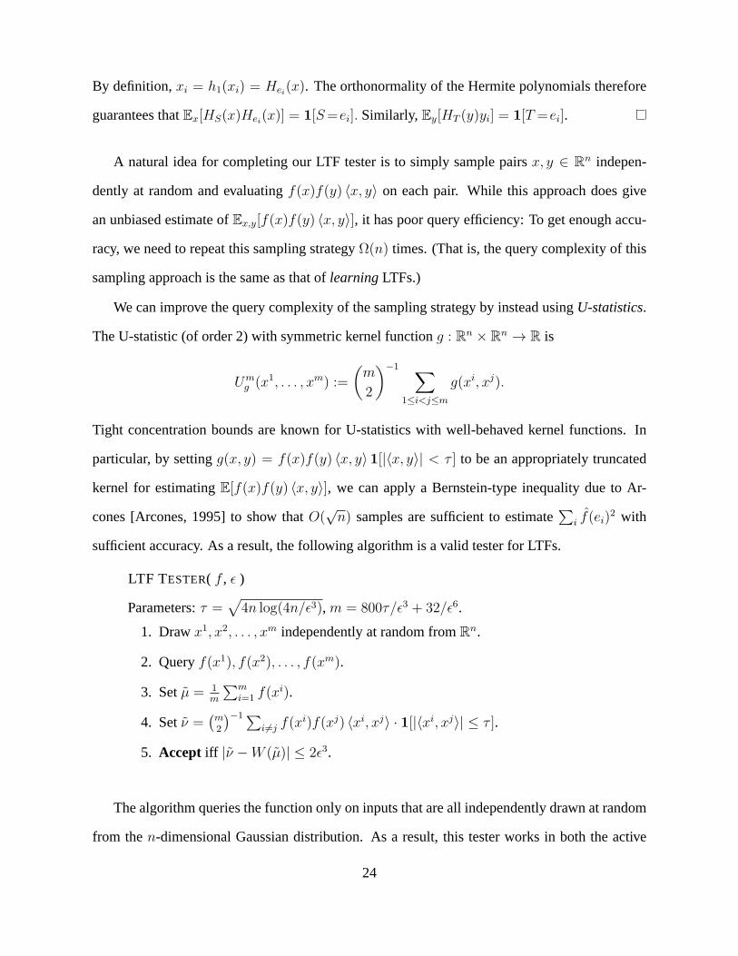
A natural idea for completing our LTF tester is to simply sample pairsx, y ∈ Rn indepen-
dently at random and evaluatingf(x)f(y) 〈x, y〉 on each pair. While this approach does give
an unbiased estimate ofEx,y[f(x)f(y) 〈x, y〉], it has poor query efficiency: To get enough accu-
racy, we need to repeat this sampling strategyΩ(n) times. (That is, the query complexity of this
sampling approach is the same as that oflearningLTFs.)
We can improve the query complexity of the sampling strategyby instead usingU-statistics.
The U-statistic (of order 2) with symmetric kernel functiong : Rn × Rn → R is
Umg (x1, . . . , xm) :=
(
m
2
)−1∑
1≤i<j≤m
g(xi, xj).
Tight concentration bounds are known for U-statistics withwell-behaved kernel functions. In
particular, by settingg(x, y) = f(x)f(y) 〈x, y〉1[|〈x, y〉| < τ ] to be an appropriately truncated
kernel for estimatingE[f(x)f(y) 〈x, y〉], we can apply a Bernstein-type inequality due to Ar-
cones [Arcones, 1995] to show thatO(√n) samples are sufficient to estimate
∑
i f(ei)2 with
sufficient accuracy. As a result, the following algorithm isa valid tester for LTFs.
LTF TESTER( f , ǫ )
Parameters:τ =√
4n log(4n/ǫ3),m = 800τ/ǫ3 + 32/ǫ6.
1. Drawx1, x2, . . . , xm independently at random fromRn.
2. Queryf(x1), f(x2), . . . , f(xm).
3. Setµ = 1m
∑mi=1 f(x
i).
4. Setν =(
m2
)−1∑
i 6=j f(xi)f(xj) 〈xi, xj〉 · 1[|〈xi, xj〉| ≤ τ ].
5. Accept iff |ν −W (µ)| ≤ 2ǫ3.
The algorithm queries the function only on inputs that are all independently drawn at random
from then-dimensional Gaussian distribution. As a result, this tester works in both the active
24

and passive testing models. For the complete proof of the correctness of the algorithm, see
Appendix 2.8.
2.4 Testing Disjoint Unions of Testable Properties
We now show that active testing has the feature that a disjoint union of testable properties is
testable, with a number of queries that is independent of thesize of the union; this feature does
not hold for passive testing. In addition to providing insight into the distinction between the
two models, this fact will be useful in our analysis of semi-supervised learning-based properties
mentioned below and discussed more fully in Appendix 2.11.
Specifically, given propertiesP1, . . . ,PN over domainsX1, . . . , XN , define their disjoint
unionP over domainX = (i, x) : i ∈ [N ], x ∈ Xi to be the set of functionsf such that
f(i, x) = fi(x) for somefi ∈ Pi. In addition, for any distributionD overX, defineDi to be the
conditional distribution overXi when the first component isi. If eachPi is testable overDi then
P is testable overD with only small overhead in the number of queries:
Theorem 2.12.Given propertiesP1, . . . ,PN , if eachPi is testable overDi with q(ǫ) queries and
U(ǫ) unlabeled samples, then their disjoint unionP is testable over the combined distributionD
withO(q(ǫ/2) · (log3 1ǫ)) queries andO(U(ǫ/2) · (N
ǫlog3 1
ǫ)) unlabeled samples.
Proof. See Appendix 2.9.
As a simple example, considerPi to contain just the constant functions1 and0. In this case,
P is equivalent to what is often called the “cluster assumption,” used in semi-supervised and
active learning [Chapelle, Schlkopf, and Zien, 2006, Dasgupta, 2011], that if data lies in some
number of clearly identifiable clusters, then all points in the same cluster should have the same
label. Here, eachPi individually is easily testable (even passively) withO(1/ǫ) labeled samples,
so Theorem 2.12 implies the cluster assumption is testable with poly(1/ǫ) queries.6 However, it
6Since thePi are so simple in this case, one can actually test with onlyO(1/ǫ) queries.
25

is not hard to see that passive testing withpoly(1/ǫ) samples is not possible and in fact requires
Ω(√N/ǫ) labeled examples.7
We build on this to produce testers for other properties often used in semi-supervised learning.
In particular, we prove the following result about testing the margin property (See Appendix 2.11
for definitions and analysis).
Theorem 2.13.For anyγ, γ′ = γ(1− 1/c) for constantc > 1, for data in the unit ball inRd for
constantd, we can distinguish the case thatDf has marginγ from the case thatDf is ǫ-far from
marginγ′ using Active Testing withO(1/(γ2dǫ2)) unlabeled examples andO(1/ǫ) label requests.
2.5 General Testing Dimensions
The previous sections have discussed upper and lower boundsfor a variety of classes. Here,
we define notions oftesting dimensionfor passive and active testing that characterize (up to
constant factors) the number of labels needed for testing tosucceed, in the corresponding testing
protocols. These will be distribution-specific notions (like SQ dimension in learning), so let us
fix some distributionD over the instance spaceX, and furthermore fix some valueǫ defining our
goal. I.e., our goal is to distinguish the case thatdistD(f,P) = 0 from the casedistD(f,P) ≥ ǫ.
For a given setS of unlabeled points, and a distributionπ over boolean functions, defineπS
to be the distribution over labelings ofS induced byπ. That is, fory ∈ 0, 1|S| let πS(y) =
Prf∼π[f(S) = y]. We now use this to define a distance between distributions. Specifically, given
a set of unlabeled pointsS and two distributionsπ andπ′ over boolean functions, define
DS(π, π′) = (1/2)
∑
y∈0,1|S|
|πS(y)− π′S(y)|,
7Specifically, suppose region 1 has1− 2ǫ probability mass withf1 ∈ P1, and suppose the other regions equally
share the remaining2ǫ probability mass and either (a) are each pure but random (sof ∈ P) or (b) are each 50/50
(so f is ǫ-far fromP). Distinguishing these cases requires seeing at least two points with the same indexi 6= 1,
yielding theΩ(√N/ǫ) bound.
26

to be the variation distance betweenπ andπ′ induced byS. Finally, letΠ0 be the set of all
distributionsπ over functions inP, and let setΠǫ be the set of all distributionsπ′ in which a
1− o(1) probability mass is over functions at leastǫ-far fromP. We are now ready to formulate
our notions of dimension.
Definition 2.14. Define the passive testing dimension,dpassive, as the largestq ∈ N such that,
supπ∈Π0
supπ′∈Πǫ
PrS∼Dq
(DS(π, π′) > 1/4) ≤ 1/4.
That is, there exist distributionsπ andπ′ such that a random setS of dpassive examples has a
reasonable probability (at least3/4) of having the property that one cannot reliably distinguish
a random function fromπ versus a random function fromπ′ from just the labels ofS. From the
definition it is fairly immediate thatΩ(dpassive) examples arenecessaryfor passive testing; in
fact,O(dpassive) are sufficient as well.
Theorem 2.15.The sample complexity of passive testing isΘ(dpassive).
Proof. See Appendix 2.10.
For the case of active testing, there are two complications.First, the algorithms can examine
their entirepoly(n)-sized unlabeled sample before deciding which points to query, and secondly
they may in principle determine the next query based on the responses to the previous ones (even
though all our algorithmic results do not require this feature). If we merely want to distinguish
those properties that are actively testable withO(1) queries from those that are not, then the
second complication disappears and the first is simplified aswell, and the following coarse notion
of dimension suffices.
Definition 2.16. Define the coarse active testing dimension,dcoarse, as the largestq ∈ N such
that,
supπ∈Π0
supπ′∈Πǫ
PrS∼Dq
(DS(π, π′) > 1/4) ≤ 1/nq.
Theorem 2.17. If dcoarse = O(1) the active testing ofP can be done withO(1) queries, and if
dcoarse = ω(1) then it cannot.
27

Proof. See Appendix 2.10.
To achieve a more fine-grained characterization of active testing we consider a slightly more
involved quantity, as follows. First, recall that given an unlabeled sampleU and distributionπ
over functions, we defineπU as the induced distribution over labelings ofU . We can view this as
a distribution overunlabeledexamples in0, 1|U |. Now, given two distributions over functions
π, π′, defineFair(π, π′, U) to be the distribution overlabeledexamples(y, ℓ) defined as: with
probability1/2 choosey ∼ πU , ℓ = 1 and with probability1/2 choosey ∼ π′U , ℓ = 0. Thus, for
a given unlabeled sampleU , the setsΠ0 andΠǫ define aclassof fair distributions over labeled
examples. The active testing dimension, roughly, asks how well this class can be approximated
by the class of low-depth decision trees. Specifically, letDTk denote the class of decision trees
of depth at mostk. The active testing dimension for a given numberu of allowed unlabeled
examples is as follows:
Definition 2.18. Given a numberu = poly(n) of allowed unlabeled examples, we define the
active testing dimension,dactive(u), as the largestq ∈ N such that
supπ∈Π0
supπ′∈Πǫ
PrU∼Du
(err∗(DTq,Fair(π, π′, U)) < 1/4) ≤ 1/4,
whereerr∗(H,P ) is the error of the optimal function inH with respect to data drawn from
distributionP over labeled examples.
Theorem 2.19. Active testing with failure probability18
usingu unlabeled examples requires
Ω(dactive(u)) label queries, and furthermore can be done withO(u) unlabeled examples and
O(dactive(u)) label queries.
Proof. See Appendix 2.10.
We now use these notions of dimension to prove lower bounds for testing several properties.
28

2.5.1 Application: Dictator functions
We now prove Theorem 2.3 that active testing of dictatorships over the uniform distribution re-
quiresΩ(log n) queries by proving aΩ(log n) lower bound ondactive(u) for anyu = poly(n); in
fact, this result holds even for the specific choice ofπ′ as random noise (the uniform distribution
over all functions).
Proof of Theorem 2.3.Defineπ andπ′ to be uniform distributions over the dictator functions and
over all boolean functions, respectively. In particular,π is the distribution obtained by choosing
i ∈ [n] uniformly at random and returning the functionf : 0, 1n → 0, 1 defined byf(x) =
xi. Fix S to be a set ofq vectors in0, 1n. This set can be viewed as aq × n boolean-valued
matrix. We writec1(S), . . . , cn(S) to represent the columns of this matrix. For anyy ∈ 0, 1q,
πS(y) =|i ∈ [n] : ci(S) = y|
nand π′
S(y) = 2−q.
By Lemma 2.21, to prove thatdactive ≥ 12log n, it suffices to show that whenq < 1
2log n
andU is a set ofnc vectors chosen uniformly and independently at random from0, 1n, then
with probability at least34, every setS ⊆ U of size |S| = q and everyy ∈ 0, 1q satisfy
πS(y) ≤ 652−q. (This is like a stronger version ofdcoarse whereDS(π, π
′) is replaced with anL∞
distance.)
Consider a setS of q vectors chosen uniformly and independently at random from0, 1n.
For any vectory ∈ 0, 1q, the expected number of columns ofS that are equal toy is n2−q.
Since the columns are drawn independently at random, Chernoff bounds imply that
Pr[
πS(y) >652−q]
≤ e−( 15)2n2−q/3 < e−
175
n2−q
.
By the union bound, the probability that there exists a vectory ∈ 0, 1q such that more than
65n2−q columns ofS are equal toy is at most2qe−
175
n2−q. Furthermore, whenU is defined as
above, we can apply the union bound once again over all subsetsS ⊆ U of size|S| = q to obtain
Pr[∃S, y : πS(y) >652−q] < ncq · 2q · e− 1
75n2−q
. Whenq ≤ 12log n, this probability is bounded
29

above byec2log2 n+ 1
2logn− 1
75
√n, which is less than1
4whenn is large enough, as we wanted to
show.
2.5.2 Application: LTFs
The testing dimension also lets us prove the lower bounds in Theorem 2.5 regarding the query
complexity for testing linear threshold functions. Specifically, those bounds follow directly from
the following result.
Theorem 2.20.For linear threshold functions under the standardn-dimensional Gaussian dis-
tribution, dpassive = Ω(√
n/ log(n)) anddactive = Ω((n/ log(n))1/3).
Let us give a brief overview of the strategies used to obtain thedpassive anddactive bounds.
The complete proofs for both results, as well as a simpler proof thatdcoarse = Ω((n/ log n)1/3),
can be found in Appendix 2.10.4.
For both results, we setπ to be a distribution over LTFs obtained by choosingw ∼ N (0, In×n)
and outputtingf(x) = sgn(w · x). Setπ′ to be the uniform distribution over all functions—i.e.,
for anyx ∈ Rn, the value off(x) is uniformly drawn from0, 1 and is independent of the value
of f on other inputs.
To bounddpassive, we bound the total variation distance between the distribution ofXw/√n
givenX, and the standard normalN (0, In×n). If this distance is small, then so must be the
distance between the distribution ofsgn(Xw) and the uniform distribution over label sequences.
Our strategy for boundingdactive is very similar to the one we used to prove the lower bound
on the query complexity for testing dictator functions in the last section. Again, we want to
apply Lemma 2.21. Specifically, we want to show that whenq ≤ o((n/ log(n))1/3) andU is a
set ofnc vectors drawn independently from then-dimensional standard Gaussian distribution,
then with probability at least34, every setS ⊆ U of size|S| = q and almost allx ∈ R
q, we have
πS(x) ≤ 652−q. The difference between this case and the lower bound for dictator functions is
that we now rely on strong concentration bounds on the spectrum of random matrices [Vershynin,
30

2012] to obtain the desired inequality.
2.6 Proof of a Property Testing Lemma
The following lemma is a generalization of a lemma that is widely used for proving lower bounds
in property testing [Fischer, 2001, Lem. 8.3]. We use this lemma to prove the lower bounds on
the query complexity for testing dictator functions and testing linear threshold functions.
Lemma 2.21. Let π andπ′ be two distributions on functionsX → R. Fix U ⊆ X to be a set
of allowable queries. Suppose that for anyS ⊆ U , |S| = q, there is a setES ⊆ Rq (possibly
empty) satisfyingπS(ES) ≤ 152−q such that
πS(y) <65π′S(y) for everyy ∈ R
q \ ES.
Thenerr∗(DTq,Fair(π, π′, U)) > 1/4.
Proof. Consider any decision treeA of depthq. Each internal node of the tree consists of a
queryy ∈ U and a subsetT ⊆ R such that its children are labeled byT andR \ T , respectively.
The leaves of the tree are labeled with either “accept” or “reject”, and letL be the set of leaves
labeled as accept. Each leafℓ ∈ L corresponds to a setSℓ ⊆ U q of queries and a subsetTℓ ⊆ Rℓ,
wheref : X → R leads to the leafℓ iff f(Sℓ) ∈ Tℓ. The probability thatA (correctly) accepts
an input drawn fromπ is
a1 =∑
ℓ∈L
∫
Tℓ
πSℓ(y)dy.
Similarly, the probability thatA (incorrectly) accepts an input drawn fromπ′ is
a2 =∑
ℓ∈L
∫
Tℓ
π′Sℓ(y)dy.
The difference between the two rejection probabilities is bounded above by
a1 − a2 ≤∑
ℓ∈L
∫
Tℓ\ESℓ
πSℓ(y)− π′
Sℓ(y)dy +
∑
ℓ∈L
∫
Tℓ∩ESℓ
πSℓ(y)dy.
31

The conditions in the statement of the lemma then imply that
a1 − a2 <∑
ℓ∈L
∫
Tℓ
16πSℓ
(y)dy + 56
∑
ℓ
∫
ESℓ
πSℓ(y)dy ≤ 1
3.
To complete the proof, we note thatA errs on an input drawn fromFair(π, π′, U) with probability
12(1− a1) + 1
2a2 =
12− 1
2(a1 − a2) > 1
3.
2.7 Proofs for Testing Unions of Intervals
In this section we complete the proofs of the technical results in Section 2.2.
Proposition 2.7(Restated). Fix δ > 0 and letf : [0, 1]→ 0, 1 be a union ofd intervals. Then
NSδ(f) ≤ dδ.
Proof. For any fixedb ∈ [0, 1], the probability thatx < b < y whenx ∼ U(0, 1) andy ∼
U(x− δ, x+ δ) is
Prx,y
[x < b < y] =
∫ δ
0
Pry∼U(b−t−δ,b−t+δ)
[y ≥ b]dt =
∫ δ
0
δ − t2δ
dt =δ
4.
Similarly,Prx,y[y < b < x] = δ4. So the probability thatb lies betweenx andy is at mostδ
2.
When f is the union ofd intervals,f(x) 6= f(y) only if at least one of the boundaries
b1, . . . , b2d of the intervals off lies in betweenx andy. So by the union bound,Pr[f(x) 6=
f(y)] ≤ 2d(δ/2) = dδ. Note that ifb is within distanceδ of 0 or 1, the probability is only
lower.
Lemma 2.8(Restated). Fix δ = ǫ2
32d. Letf : [0, 1]→ 0, 1 be any function with noise sensitivity
NSδ(f) ≤ dδ(1 + ǫ4). Thenf is ǫ-close to a union ofd intervals.
Proof. The proof proceeds in two steps: We first show thatf is ǫ2-close to a union ofd(1 + ǫ
2)
intervals, then we show that every union ofd(1+ ǫ2) intervals isǫ
2-close to a union ofd intervals.
32

Consider the “smoothed” functionfδ : [0, 1]→ [0, 1] defined by
fδ(x) = Ey∼δxf(y) =1
2δ
∫ x+δ
x−δ
f(y)dy.
The functionfδ is the convolution off and the uniform kernelφ : R → [0, 1] defined by
φ(x) = 12δ1[|x| ≤ δ].
Fix τ = 4ǫNSδ(f). We introduce the functiong∗ : [0, 1]→ 0, 1, ∗ by setting
g∗(x) =
1 whenfδ(x) ≥ 1− τ ,
0 whenfδ(x) ≤ τ , and
∗ otherwise
for all x ∈ [0, 1]. Finally, we defineg : [0, 1] → 0, 1 by settingg(x) = g∗(y) wherey ≤ x is
the largest value for whichg(y) 6= ∗. (If no suchy exists, we fixg(x) = 0.)
We first claim thatdist(f, g) ≤ ǫ2. To see this, note that
dist(f, g) = Prx[f(x) 6= g(x)]
≤ Prx[g∗(x) = ∗] + Pr
x[f(x) = 0 ∧ g∗(x) = 1] + Pr
x[f(x) = 1 ∧ g∗(x) = 0]
= Prx[τ < fδ(x) < 1− τ ] + Pr
x[f(x) = 0 ∧ fδ(x) ≥ 1− τ ] + Pr
x[f(x) = 1 ∧ fδ(x) ≤ τ ].
We bound the three terms on the RHS individually. For the first term, we observe thatNSδ(f, x) =
minfδ(x), 1− fδ(x) and thatExNSδ(f, x) = NSδ(f). From these identities and Markov’s in-
equality, we have that
Prx[τ < fδ(x) < 1− τ ] = Pr
x[NSδ(f, x) > τ ] <
NSδ(f)
τ=ǫ
4.
For the second term, letS ⊆ [0, 1] denote the set of pointsx wheref(x) = 0 andfδ(x) ≥ 1− τ .
Let Γ ⊆ S represent aδ-net ofS. Clearly, |Γ| ≤ 1δ. Forx ∈ Γ, letBx = (x − δ, x + δ) be a
ball of radiusδ aroundx. Sincefδ(x) ≥ 1 − τ , the intersection ofS andBx has mass at most
|S ∩ Bx| ≤ τδ. Therefore, the total mass ofS is at most|S| ≤ |Γ|τδ = τ . By the bounds on the
33

noise sensitivity off in the lemma’s statement, we therefore have
Prx[f(x) = 0 ∧ fδ(x) ≥ 1− τ ] ≤ τ ≤ ǫ
8.
Similarly, we obtain the same bound on the third term. As a result, dist(f, g) ≤ ǫ4+ ǫ
8+ ǫ
8= ǫ
2,
as we wanted to show.
We now want to show thatg is a union ofm ≤ dδ(1 + ǫ2) intervals. Each left boundary of an
interval ing occurs at a pointx ∈ [0, 1] whereg∗(x) = ∗, where the maximumy ≤ x such that
g∗(y) 6= ∗ takes the valueg∗(y) = 0, and where the minimumz ≥ x such thatg∗(z) 6= ∗ has
the valueg∗(z) = 1. In other words, for each left boundary of an interval ing, there exists an
interval(y, z) such thatfδ(y) ≤ τ , fδ(z) ≥ 1 − τ , and for eachy < x < z, fδ(x) ∈ (τ, 1 − τ).
Fix any interval(y, z). Sincefδ is the convolution off with a uniform kernel of width2δ, it
is Lipschitz continuous (with Lipschitz constant12δ
). So there existsx ∈ (y, z) such that the
conditionsfδ(x) = 12, x− y ≥ 2δ(1
2− τ), andz − x ≥ 2δ(1
2− τ) all hold. As a result,
∫ z
y
NSδ(f, t) dt =
∫ x
y
NSδ(f, t) dt+
∫ z
x
NSδ(f, t) dt ≥ 2δ(12− τ)2.
Similarly, for each right boundary of an interval ing, we have an interval(y, z) such that
∫ z
y
NSδ(f, t) dt ≥ 2δ(12− τ)2.
The intervals(y, z) for the left and right boundaries are all disjoints, so
NSδ(f) ≥2m∑
i=1
∫ zi
yiNSδ(f, t) dt ≥ 2m
δ
2(1− 2τ)2.
This means that
m ≤ dδ(1 + ǫ/4)
δ(1− 2τ)2≤ d(1 + ǫ
2)
andg is a union of at mostd(1 + ǫ2) intervals, as we wanted to show.
Finally, we want to show that any function that is the union ofm ≤ d(1 + ǫ2) intervals isǫ
2-
close to a union ofd intervals. Letℓ1, . . . , ℓm represent the lengths of the intervals ing. Clearly,
34

ℓ1 + · · ·+ ℓm ≤ 1, so there must be a setS of m− d ≤ dǫ/2 intervals inf with total length
∑
i∈Sℓi ≤
m− dm
≤ dǫ/2
d(1 + ǫ2)<ǫ
2.
Consider the functionh : [0, 1] → 0, 1 obtained by removing the intervals inS from g (i.e.,
by settingh(x) = 0 for the valuesx ∈ [b2i−1, b2i] for somei ∈ S). The functionh is a union
of d intervals anddist(g, h) ≤ ǫ2. This completes the proof, sincedist(f, h) ≤ dist(f, g) +
dist(g, h) ≤ ǫ.
2.8 Proofs for Testing LTFs
We complete the proof that LTFs can be tested withO(√n) samples in this section.
For a fixed functionf : Rn → R, defineg : Rn × Rn → R to beg(x, y) = f(x)f(y) 〈x, y〉.
Let g∗ : Rn × Rn → R be the truncation ofg defined by setting
g∗(x, y) =
f(x)f(y) 〈x, y〉 if | 〈x, y〉 | ≤√
4n log(4n/ǫ3)
0 otherwise.
Our goal is to estimateEg. The following lemma shows thatEg∗ provides a good estimate of
this value.
Lemma 2.22.Letg, g∗ : Rn × Rn → R be defined as above. Then|Eg − Eg∗| ≤ 1
2ǫ3.
Proof. For notational clarity, fixτ =√
4n log(4n/ǫ3). By the definition ofg andg∗ and with
the trivial bound|f(x)f(y) 〈x, y〉 | ≤ n we have
|Eg−Eg∗| =∣
∣
∣
∣
Prx,y
[
|〈x, y〉| > τ]
· Ex,y
[
f(x)f(y) 〈x, y〉∣
∣ |〈x, y〉| > τ]
∣
∣
∣
∣
≤ n ·Prx,y
[
|〈x, y〉| > τ]
.
The right-most term can be bounded with a standard Chernoff argument. By Markov’s inequality
and the independence of the variablesx1, . . . , xn, y1, . . . , yn,
Prx,y
[
〈x, y〉 > τ]
= Pr[
et〈x,y〉 > etτ]
≤ Eet〈x,y〉
etτ=
∏ni=1 Ee
txiyi
etτ.
35

The moment generating function of a standard normal random variable isEety = et2/2, so
Exi,yi
[
etxiyi]
= Exi
[
Eyietxiyi]
= Exie(t
2/2)x 2i .
Whenx ∼ N (0, 1), the random variablex2 has aχ2 distribution with 1 degree of freedom. The
moment generating function of this variable isEetx2=√
11−2t
=√
1 + 2t1−2t
for any t < 12.
Hence,
Exie(t
2/2)x 2i ≤
√
1 +t2
1− t2 ≤ et2
2(1−t2)
for anyt < 1. Combining the above results and settingt = τ2n
yields
Prx,y
[
〈x, y〉 > τ]
≤ ent2
2(1−t2)−tτ ≤ e−
τ2
4n = ǫ3
4n.
The same argument shows thatPr[〈x, y〉 < −τ ] ≤ ǫ3
4nas well.
The reason we consider the truncationg∗ is that its smallerℓ∞ norm will enable us to apply
a strong Bernstein-type inequality on the concentration of measure of the U-statistic estimate of
Eg∗.
Lemma 2.23(Arcones [Arcones, 1995]). For a symmetric functionh : Rn × Rn → R, letΣ2 =
Ex[Ey[h(x, y)]2] − Ex,y[h(x, y)]
2, let b = ‖h − Eh‖∞, and letUm(h) be a random variable ob-
tained by drawingx1, . . . , xm independently at random and settingUm(h) =(
m2
)−1∑
i<j h(xi, xj).
Then for everyt > 0,
Pr[|Um(h)− Eh| > t] ≤ 4 exp
(
mt2
8Σ2 + 100bt
)
.
We are now ready to complete the proof of the upper bound of Theorem 2.5.
Theorem 2.24(Upper bound in Theorem 2.5, restated). Linear threshold functions can be tested
over the standardn-dimensional Gaussian distribution withO(√n log n) queries in both the
active and passive testing models.
Proof. Consider the LTF-TESTERalgorithm. When the estimatesµ andν satisfy
|µ− Ef | ≤ ǫ3 and |ν − E[f(x)f(y) 〈x, y〉]| ≤ ǫ3,
36

Lemmas 2.10 and 2.11 guarantee that the algorithm correctlydistinguishes LTFs from functions
that are far from LTFs. To complete the proof, we must therefore show that the estimates are
within the specified error bounds with probability at least2/3.
The valuesf(x1), . . . , f(xm) are independent−1, 1-valued random variables. By Hoeffd-
ing’s inequality,
Pr[|µ− Ef | ≤ ǫ3] ≥ 1− 2e−ǫ6m/2 = 1− 2e−O(√n).
The estimateν is a U-statistic with kernelg∗ as defined above. This kernel satisfies
‖g∗ − Eg∗‖∞ ≤ 2‖g∗‖∞ = 2√
4n log(4n/ǫ3)
and
Σ2 ≤ Ey
[
Ex[g∗(x, y)]2
]
= Ey
[
Ex[f(x)f(y) 〈x, y〉1[|〈x, y〉| ≤ τ ]]2]
.
For any two functionsφ, ψ : Rn → R, whenψ is 0, 1-valued the Cauchy-Schwarz in-
equality implies thatEx[φ(x)ψ(x)]2 ≤ Ex[φ(x)]Ex[φ(x)ψ(x)
2] = Ex[φ(x)]Ex[φ(x)ψ(x)] and
soEx[φ(x)ψ(x)]2 ≤ Ex[φ(x)]. Applying this inequality to the expression forΣ2 gives
Σ2 ≤ Ey
[
Ex[f(x)f(y) 〈x, y〉]2]
= Ey
[(
n∑
i=1
f(y)yiEx[f(x)xi])2]
=∑
i,j
f(ei)f(ej)Ey[yiyj] =n∑
i=1
f(ei)2.
By Parseval’s identity, we have∑
i f(ei)2 ≤ ‖f‖22 = ‖f‖22 = 1. Lemmas 2.22 and 2.23 imply
that
Pr[|ν − Eg| ≤ ǫ3] = Pr[|ν − Eg∗| ≤ 12ǫ3] ≥ 1− 4e
− mt2
8+200√
n log(4n/ǫ3)t ≥ 1112.
The union bound completes the proof of correctness.
2.9 Proofs for Testing Disjoint Unions
Theorem 2.12(Restated). Given propertiesP1, . . . ,PN , if eachPi is testable overDi with q(ǫ)
queries andU(ǫ) unlabeled samples, then their disjoint unionP is testable over the combined
distributionD withO(q(ǫ/2) · (log3 1ǫ)) queries andO(U(ǫ/2) · (N
ǫlog3 1
ǫ)) unlabeled samples.
37

Proof. Let p = (p1, . . . , pN) denote the mixing weights for distributionD; that is, a random
draw fromD can be viewed as selectingi from distributionp and then selectingx fromDi. We
are given that eachPi is testable with failure probability1/3 using usingq(ǫ) queries andU(ǫ)
unlabeled samples. By repetition, this implies that each is testable with failure probabilityδ using
qδ(ǫ) = O(q(ǫ) log(1/δ)) queries andUδ(ǫ) = O(U(ǫ) log(1/δ)) unlabeled samples, where we
will set δ = ǫ2. We now test propertyP as follows:
For ǫ′ = 1/2, 1/4, 1/8, . . . , ǫ/2 do:
RepeatO( ǫ′
ǫlog(1/ǫ)) times:
1. Choose a random(i, x) fromD.
2. Sample until eitherUδ(ǫ′) samples have been drawn fromDi or (8N/ǫ)Uδ(ǫ
′)
samples total have been drawn fromD, whichever comes first.
3. In the former case, run the tester for propertyPi with parameterǫ′, making
qδ(ǫ′) queries. If the tester rejects, then reject.
If all runs have accepted, then accept.
First to analyze the total number of queries and samples, since we can assumeq(ǫ) ≥ 1/ǫ and
U(ǫ) ≥ 1/ǫ, we haveqδ(ǫ′)ǫ′/ǫ = O(qδ(ǫ/2)) andUδ(ǫ′)ǫ′/ǫ = O(Uδ(ǫ/2)) for ǫ′ ≥ ǫ/2. Thus,
the total number of queries made is at most
∑
ǫ′
qδ(ǫ/2) log(1/ǫ) = O
(
q(ǫ/2) · log3 1ǫ
)
and the total number of unlabeled samples is at most
∑
ǫ′
8N
ǫUδ(ǫ/2) log(1/ǫ) = O
(
U(ǫ/2)N
ǫlog3
1
ǫ
)
.
Next, to analyze correctness, if indeedf ∈ P then each call to a tester rejects with probability
at mostδ so the overall failure probability is at most(δ/ǫ) log2(1/ǫ) < 1/3; thus it suffices to
analyze the case thatdistD(f,P) ≥ ǫ.
38

If distD(f,P) ≥ ǫ then∑
i:pi≥ǫ/(4N) pi · distDi(fi,Pi) ≥ 3ǫ/4. Moreover, for indicesi such that
pi ≥ ǫ/(4N), with high probability Step 2 drawsUδ(ǫ′) samples, so we may assume for such
indices the tester forPi is indeed run in Step 3. LetI = i : pi ≥ ǫ/(4N) anddistDi(fi,Pi) ≥
ǫ/2. Thus, we have∑
i∈Ipi · distDi
(fi,Pi) ≥ ǫ/4.
Let Iǫ′ = i ∈ I : distDi(fi,Pi) ∈ [ǫ′, 2ǫ′]. Bucketing the above summation by valuesǫ′ in this
way implies that for some valueǫ′ ∈ ǫ/2, ǫ, 2ǫ, . . . , 1/2, we have:
∑
i∈Iǫ′pi ≥ ǫ/(8ǫ′ log(1/ǫ)).
This in turn implies that with probability at least2/3, the run of the algorithm for this value ofǫ′
will find such ani and reject, as desired.
2.10 Proofs for Testing Dimensions
2.10.1 Passive Testing Dimension (proof of Theorem 2.15)
Lower bound: By design,dpassive is a lower bound on the number of examples needed for
passive testing. In particular, ifDS(π, π′) ≤ 1/4, and if the target is with probability1/2 chosen
fromπ and with probability1/2 chosen fromπ′, even the Bayes optimal tester will fail to identify
the correct distribution with probability12
∑
y∈0,1|S| min(πS(y), π′S(y)) =
12(1 − DS(π, π
′)) ≥
3/8. The definition ofdpassive implies that there existπ ∈ Π0, π′ ∈ Πǫ such thatPrS(DS(π, π′) ≤
1/4) ≥ 3/4. Sinceπ′ has a1 − o(1) probability mass on functions that areǫ-far fromP, this
implies that over random draws ofS andf , the overall failure probability of any tester is at least
(1− o(1))(3/8)(3/4) > 1/4. Thus, at leastdpassive + 1 random labeled examples are required if
we wish to guarantee error at most1/4. This in turn impliesΩ(dpassive) examples are needed to
guarantee error at most1/3.
39

Upper bound: We now argue thatO(dpassive) examples aresufficientfor testing as well. Toward
this end, consider the following natural testing game. The adversary chooses a functionf such
that eitherf ∈ P or distD(f,P) ≥ ǫ. The tester picks a functionA that maps labeled samples
of sizek to accept/reject. That is,A is a deterministic passive testing algorithm. The payoff to
the tester is the probability thatA is correct whenS is chosen iid fromD and labeled byf .
If k > dpassive then (by definition ofdpassive) we know that for any distributionπ overf ∈ P
and any distributionπ′ overf that areǫ-far fromP, we havePrS∼Dk(DS(π, π′) > 1/4) > 1/4.
We now need to translate this into a statement about the valueof the game. The key fact we can
use is that if the adversary uses distributionαπ + (1 − α)π′ (i.e., with probabilityα it chooses
from π and with probability1−α it chooses fromπ′), then the Bayes optimal predictor has error
exactly
∑
y
min(απS(y), (1− α)π′S(y)) ≤ max(α, 1− α)
∑
y
min(πS(y), π′S(y)),
while
∑
y
min(πS(y), π′S(y)) = 1− (1/2)
∑
y
|πS(y)− π′S(y)| = 1−DS(π, π
′),
so that the Bayes risk is at mostmax(α, 1− α)(1−DS(π, π′)). Thus, for anyα ∈ [7/16, 9/16],
if DS(π, π′) > 1/4, the Bayes risk is less than(9/16)(3/4) = 27/64. Furthermore, anyα /∈
[7/16, 9/16] has Bayes risk at most7/16. Thus, sinceDS(π, π′) > 1/4 with probability> 1/4
(and if DS(π, π′) ≤ 1/4 then the error probability of the Bayes optimal predictor is at most
1/2), for any mixed strategy of the adversary, the Bayes optimal predictor has risk less than
(1/4)(7/16) + (3/4)(1/2) = 31/64.
Now, applying the minimax theorem we get that fork = dpassive + 1, there exists a mixed
strategyA for the tester such that for any function chosen by the adversary, the probability the
tester is correct is at least1/2 + γ for a constantγ > 0 (namely,1/64). We can now boost the
correctness probability using a constant-factor larger sample. Specifically, letm = c·(dpassive+1)
for some constantc, and consider a sampleS of sizem. The tester simply partitions the sample
40
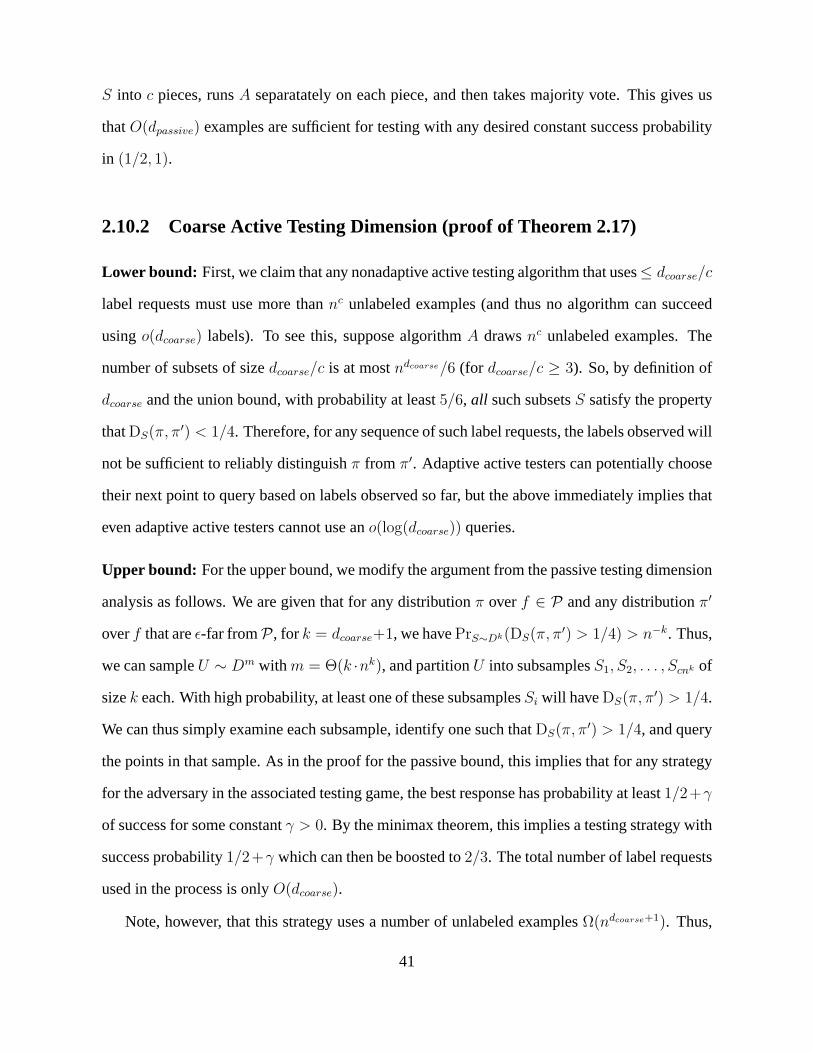
S into c pieces, runsA separatately on each piece, and then takes majority vote. This gives us
thatO(dpassive) examples are sufficient for testing with any desired constant success probability
in (1/2, 1).
2.10.2 Coarse Active Testing Dimension (proof of Theorem 2.17)
Lower bound: First, we claim that any nonadaptive active testing algorithm that uses≤ dcoarse/c
label requests must use more thannc unlabeled examples (and thus no algorithm can succeed
usingo(dcoarse) labels). To see this, suppose algorithmA drawsnc unlabeled examples. The
number of subsets of sizedcoarse/c is at mostndcoarse/6 (for dcoarse/c ≥ 3). So, by definition of
dcoarse and the union bound, with probability at least5/6, all such subsetsS satisfy the property
thatDS(π, π′) < 1/4. Therefore, for any sequence of such label requests, the labels observed will
not be sufficient to reliably distinguishπ from π′. Adaptive active testers can potentially choose
their next point to query based on labels observed so far, butthe above immediately implies that
even adaptive active testers cannot use ano(log(dcoarse)) queries.
Upper bound: For the upper bound, we modify the argument from the passive testing dimension
analysis as follows. We are given that for any distributionπ overf ∈ P and any distributionπ′
overf that areǫ-far fromP, for k = dcoarse+1, we havePrS∼Dk(DS(π, π′) > 1/4) > n−k. Thus,
we can sampleU ∼ Dm withm = Θ(k ·nk), and partitionU into subsamplesS1, S2, . . . , Scnk of
sizek each. With high probability, at least one of these subsamplesSi will haveDS(π, π′) > 1/4.
We can thus simply examine each subsample, identify one suchthatDS(π, π′) > 1/4, and query
the points in that sample. As in the proof for the passive bound, this implies that for any strategy
for the adversary in the associated testing game, the best response has probability at least1/2+γ
of success for some constantγ > 0. By the minimax theorem, this implies a testing strategy with
success probability1/2+γ which can then be boosted to2/3. The total number of label requests
used in the process is onlyO(dcoarse).
Note, however, that this strategy uses a number of unlabeledexamplesΩ(ndcoarse+1). Thus,
41

this only implies an active tester fordcoarse = O(1). Nonetheless, combining the upper and lower
bounds yields Theorem 2.17.
2.10.3 Active Testing Dimension (proof of Theorem 2.19)
Lower bound: for a given sampleU , we can think of an adaptive active tester as a decision
tree, defined based on which example it would request the label of next given that the previous
requests have been answered in any given way. A tester makingk queries would yield a decision
tree of depthk. By definition ofdactive(u), with probability at least3/4 (over choice ofU ), any
such tester has error probability at least(1/4)(1 − o(1)) over the choice off . Thus, the overall
failure probability is at least(3/4)(1/4)(1− o(1) > 1/8.
Upper bound: We again consider the natural testing game. We are given thatfor any mixed
strategy of the adversary with equal probability mass on functions inP and functionsǫ-far from
P, the best response of the tester has expected payoff at least(1/4)(3/4) + (3/4)(1/2) = 9/16.
This in turn implies that for any mixed strategy at all, the best response of the tester has expected
payoff at least33/64 (if the adversary puts more than17/32 probability mass on either type
of function, the tester can just guess that type with expected payoff at least17/32, else it gets
payoff at least(1 − 1/16)(9/16) > 33/64). By the minimax theorem, this implies existence of
a randomized strategy for the tester with at least this payoff. We then boost correctness using
c · u samples andc · dactive(u) queries, running the testerc times on disjoint samples and taking
majority vote.
2.10.4 Lower Bounds for Testing LTFs (proof of Theorem 2.20)
We complete the proofs for the lower bounds on the query complexity for testing linear threshold
functions in the active and passive models. This proof has three parts. First, in Section 2.10.4, we
introduce some preliminary (technical) results that will be used to prove the lower bounds on the
passive and coarse dimensions of testing LTFs. In Section 2.10.4, we introduce some more pre-
42

liminary results regarding random matrices that we will useto bound the active dimension of the
class. Finally, in Section 2.10.4, we put it all together andcomplete the proof of Theorem 2.20.
Preliminaries for dpassive and dcoarse
Fix anyK. Let the datasetX = x1, x2, · · · , xK be sampled iid according to the uniform
distribution on−1,+1n and letX ∈ RK×n be the corresponding data matrix.
Supposew ∼ N(0, In×n). We let
z = Xw,
and note that the conditional distribution ofz givenX is normal with mean0 and (X-dependent)
covariance matrix, which we denote byΣ. Further applying threshold function toz givesy as
the predicted label vector of an LTF.
Lemma 2.25. For any matrixB, log(det(B)) = Tr(log(B)), wherelog(B) is the matrix expo-
nential ofB.
Proof. From [Higham, 2008], we know since every eigenvalue ofA corresponds to the eigen-
value ofexp(A), thus
det(exp(A)) = exp(Tr(A)) (2.1)
whereexp(A) is the matrix exponential ofA. Taking logarithm of both sides of (2.1), we get
log(det(exp(A))) = Tr(A) (2.2)
LetB = exp(A) (thusA = log(B)). Then (2.2) can rewritten aslog(det(B)) = Tr(logB).
Lemma 2.26. For sufficiently largen, and a valueK = Ω(√
n/ log(K/δ)), with probability at
least1− δ (overX),
‖P(z/√n)|X −N(0, I)‖ ≤ 1/4.
43

Proof. Let l be the feature index. For a pairxi andxj,
P(∣
∣
∣|l : xil = xjl| −
n
2
∣
∣
∣>
√
n log 2δ
2) ≤ δ
By Hoeffding Inequality, with probability1− δ,
xTi xj = |l : xil = xjl| − |l : xil 6= xjl|
= 2|l : xil = xjl| − n ∈
−2
√
n log 2δ
2, 2
√
n log 2δ
2
By union bound,
P
(
∃i, j, such thatxTi xj 6∈
[
−√
2n log2K2
δ,
√
2n log2K2
δ
])
≤ K2 δ
K2= δ (2.3)
For the remainder of the proof we suppose the (probability1− δ) event
∀i, j,xTi xj ∈
[
−√
2n log(2K2/δ),√
2n log(2K2/δ)]
occurs.
Cov(zi/√n, zj/
√n|X) =
E[zizj|X]
n
=1
nE
[
(n∑
l=1
wl · xil)(n∑
l=1
wl · xjl)|X]
=1
nE
[
n,n∑
l,m=1,1
wlwmxilxjm|X]
=1
nE
[
∑
l
w2l xilxjl|X
]
=1
nE
[
∑
l
xilxjl|X]
=1
n
∑
l
xilxjl =1
nxTi xj ∈
[
−√
2 log(2K2/δ)
n,
√
2 log(2K2/δ)
n
]
becauseE[wlwm] = 0 (for l 6= m) andE[w2l ] = 1. Let β =
√
2 log(2K2/δ)n
. ThusΣ is aK ×K
matrix, withΣii = 1 for i = 1, · · · , K andΣij ∈ [−β, β] for all i 6= j.
Let P1 = N(0,ΣK×K) andP2 = N(0, IK×K). As the density
p1(z) =1
√
(2π)Kdet(Σ)exp(−1
2zTΣ−1z)
44

and the density
p2(z) =1
√
(2π)Kexp(−1
2zTz)
ThenL1 distance between the two distributionsP1 andP2
|dP2 − dP1| ≤ 2√
K(P1, P2) = 2√
(1/2) log det(Σ),
where this last equality is by [Davis and Dhillon, 2006]. By Lemma 2.25,log(det(Σ)) =
Tr(log(Σ)). WriteA = Σ− I. By the Taylor series
log(I + A) = −∞∑
i=1
1
i(I − (I + A))i = −
∞∑
i=1
1
i(−A)i
Thus Tr(log(I + A)) =∞∑
i=1
1
iT r((−A)i). (2.4)
Every entry inAi can be expressed as a sum of at mostKi−1 terms, each of which can
be expressed as a product of exactlyi entries fromA. Thus, every entry inAi is in the range
[−Ki−1βi, Ki−1βi]. This meansTr(Ai) ≤ Kiβi. Therefore, ifKβ < 1/2, sinceTr(A) = 0,
the expansion ofTr(log(I + A)) ≤∑∞i=2K
iβi = O(
K2 log(K/δ)n
)
.
In particular, for someK = Ω(√
n/ log(K/δ)), Tr(log(I +A)) is bounded by the appropri-
ate constant to obtain the stated result.
Preliminaries for dactive
Given ann×mmatrixA with real entriesai,ji∈[n],j∈[m], theadjoint (or transpose– the two are
equivalent sinceA contains only real values) ofA is them × n matrixA∗ whose(i, j)-th entry
equalsaj,i. Let us writeλ1 ≥ λ2 ≥ · · · ≥ λm to denote the eigenvalues of√A∗A. These values
are thesingular valuesof A. The matrixA∗A is positive semidefinite, so the singular values of
A are all non-negative. We writeλmax(A) = λ1 andλmin(A) = λm to represent its largest and
smallest singular values. Finally, theinduced norm(or operator norm) of A is
‖A‖ = maxx∈Rm\0
‖Ax‖2‖x‖2
= maxx∈Rm:‖x‖22=1
‖Ax‖2.
45

For more details on these definitions, see any standard linear algebra text (e.g., [Shilov, 1977]).
We will also use the following strong concentration bounds on the singular values of random
matrices.
Lemma 2.27(See [Vershynin, 2012, Cor. 5.35]). LetA be ann × m matrix whose entries are
independent standard normal random variables. Then for anyt > 0, the singular values ofA
satisfy√n−√m− t ≤ λmin(A) ≤ λmax(A) ≤
√n+√m+ t (2.5)
with probability at least1− 2e−t2/2.
The proof of this lemma follows from Talagrand’s inequalityand Gordon’s Theorem for
Gaussian matrices. See [Vershynin, 2012] for the details. The lemma implies the following
corollary which we will use in the proof of our theorem.
Corollary 2.28. Let A be ann × m matrix whose entries are independent standard normal
random variables. For any0 < t <√n−√m, them×mmatrix 1
nA∗A satisfies both inequalities
∥
∥
1nA∗A− I
∥
∥ ≤ 3
√m+ t√n
and det(
1nA∗A
)
≥ e−m
(
(√m+t)2
n+2
√m+t√n
)
(2.6)
with probability at least1− 2e−t2/2.
Proof. When there exists0 < z < 1 such that1 − z ≤ 1√nλmax(A) ≤ 1 + z, the identity
1√nλmax(A) = ‖ 1√
nA‖ = max‖x‖22=1 ‖ 1√
nAx‖2 implies that
1− 2z ≤ (1− z)2 ≤ max‖x‖22=1
∥
∥
∥
1√nAx∥
∥
∥
2
2≤ (1 + z)2 ≤ 1 + 3z.
These inequalities and the identity‖ 1nA∗A − I‖ = max‖x‖22=1 ‖ 1√
nAx‖22 − 1 imply that−2z ≤
‖ 1nA∗A− I‖ ≤ 3z. Fixing z =
√m+t√n
and applying Lemma 2.27 completes the proof of the first
inequality.
Recall thatλ1 ≤ · · · ≤ λm are the eigenvalues of√A∗A. Then
det( 1nA∗A) =
det(√A∗A)2
n=
(λ1 · · ·λm)2n
≥(
λ 21
n
)m
=
(
λmin(A)2
n
)m
.
46

Lemma 2.27 and the elementary inequality1+x ≤ ex complete the proof of the second inequal-
ity.
Proof of Theorem 2.20
Theorem 2.20 (Restated). For linear threshold functions under the uniform distribution on
−1, 1n, dpassive = Ω(√
n/ log(n)) anddactive = Ω((n/ log(n))1/3).
Proof. Let K be as in Lemma 2.26 forδ = 1/4. Let D = (x1, y1), . . . , (xK , yK) denote
the sequence of labeled data points under the random LTF based onw. Furthermore, letD′ =
(x1, y′1), . . . , (xK , y′K) denote the sequence of labeled data points under a target function that
assigns an independent random label to each data point. Alsolet zi = (1/√n)wTxi, and let
z′ ∼ N(0, IK×K). LetE = (x1, z1), . . . , (xK , zK) andE ′ = (x1, z′1), . . . , (xK , z′K). Note
that we can think ofyi andy′i as being functions ofzi andz′i, respectively. Thus, lettingX =
x1, . . . , xK, by Lemma 2.26, with probability at least3/4,
‖PD|X − PD′|X‖ ≤ ‖PE|X − PE′|X‖ ≤ 1/4.
This suffices for the claim thatdpassive = Ω(K) = Ω(√
n/ log(n)).
Next we turn to the lower bound ondactive. Let us now introduce two distributionsDyes
andDno over linear threshold functions and functions that (with high probability) are far from
linear threshold functions, respectively. We draw a function f from Dyes by first drawing a
vectorw ∼ N (0, In×n) from then-dimensional standard normal distribution. We then define
f : x 7→ sgn( 1√nx · w). To draw a functiong fromDno, we defineg(x) = sgn(yx) where each
yx variable is drawn independently from the standard normal distributionN (0, 1).
Let X ∈ Rn×q be a random matrix obtained by drawingq vectors from then-dimensional
normal distributionN (0, In×n) and setting these vectors to be the columns ofX. Equivalently,X
is the random matrix whose entries are independent standardnormal variables. When we viewX
as a set ofq queries to a functionf ∼ Dyes or a functiong ∼ Dno, we getf(X) = sgn( 1√nXw)
47

and g(X) = sgn(yX). Note that 1√nXw ∼ N (0, 1
nX∗X) andyX ∼ N (0, Iq×q). To apply
Lemma 2.21 it suffices to show that the ratio of the pdfs for both these random variables is
bounded by65
for all but 15
of the probability mass.
The pdfp : Rq → R of a q-dimensional random vector from the distributionNq×q(0,Σ) is
p(x) = (2π)−q2 det(Σ)−
12 e−
12xTΣ−1x.
Therefore, the ratio functionr : Rq → R between the pdfs of1√nXw and ofyX is
r(x) = det( 1nX∗X)−
12 e
12xT (( 1
nX
∗X)−1−I)x.
Note that
xT (( 1nX∗X)−1 − I)x ≤ ‖( 1
nX∗X)−1 − I‖‖x‖22 = ‖ 1nX∗X− I‖‖x‖22,
so by Lemma 2.27 with probability at least1− 2e−t2/2 we have
r(x) ≤ eq2
(
(√q+t)2
n+2
√q+t√n
)
+3√
q+t√n
‖x‖22.
By a union bound, forU ∼ N (0, In×n)u, u ∈ N with u ≥ q, the above inequality forr(x) is true
for all subsets ofU of sizeq, with probability at least1 − uq2e−t2/2. Fix q = n13/(50(ln(u))
13 )
andt = 2√
q ln(u). Thenuq2e−t2/2 ≤ 2u−q, which is< 1/4 for any sufficiently largen. When
‖x‖22 ≤ 3q then for largen, r(x) ≤ e74/625 < 65. To complete the proof, it suffices to show that
whenx ∼ N (0, Iq×q), the probability that‖x‖22 > 3q is at most152−q. The random variable‖x‖22
has aχ2 distribution withq degrees of freedom and expected valueE‖x‖22 =∑q
i=1 Ex2i = q.
Standard concentration bounds forχ2 variables imply that
Prx∼N (0,Iq×q)
[‖x‖22 > 3q] ≤ e−43q < 1
52−q,
as we wanted to show. Thus, Lemma 2.21 implieserr∗(DTq,Fair(π, π′, U)) > 1/4 holds when-
ever thisr(x) inequality is satisfied for all subsets ofU of sizeq; we have shown this happens
with probabiliity greater than3/4, so we must havedactive ≥ q.
48

If we are only interested in boundingdcoarse, the proof can be somewhat simplified. Specifi-
cally, takingδ = n−K in Lemma 2.26 implies that with probability at least1− n−K ,
‖PD|X − PD′|X‖ ≤ ‖PE|X − PE′|X‖ ≤ 1/4,
which suffices for the claim thatdcoarse = Ω(K), whereK = Ω(√
n/K log(n)): in particular,
dcoarse = Ω((n/ log(n))1/3).
2.11 Testing Semi-Supervised Learning Assumptions
We now consider testing of common assumptions made in semi-supervised learning [Chapelle,
Schlkopf, and Zien, 2006], where unlabeled data, together with assumptions about how the target
function and data distribution relate, are used to constrain the search space. As mentioned in
Section 2.4, one such assumption we can test using our generic disjoint-unions tester is the
cluster assumption, that if data lies inN identifiable clusters, then points in the same cluster
should have the same label. We can in fact achieve the following tighter bounds:
Theorem 2.29.We can test the cluster assumption with active testing usingO(N/ǫ) unlabeled
examples andO(1/ǫ) queries.
Proof. Let pi1 andpi0 denote the probability mass on positive examples and negative examples
respectively in clusteri, sopi1 + pi0 is the total probabilty mass of clusteri. Thendist(f,P) =∑
i min(pi1, pi0). Thus, a simple tester is to draw a random examplex, draw a random example
y from x’s cluster, and check iff(x) = f(y). Notice that with probabilityexactlydist(f,P),
pointx is in the minority class of its own cluster, and conditioned on this event, with probability
at least1/2, point y will have a different label. It thus suffices to repeat this processO(1/ǫ)
times. One complication is that as stated, this process might require a largeunlabeledsample,
especially ifx belongs to a clusteri such thatpi0+ pi1 is small, so that many draws are needed to
find a pointy in x’s cluster. To achieve the givenunlabeledsample bound, we initially draw an
unlabeled sample of sizeO(N/ǫ) and simply perform the above test on the uniform distribution
49

U over that sample, with distance parameterǫ/2. Standard sample complexity bounds [Vapnik,
1998] imply thatO(N/ǫ) unlabeled points are sufficient so that ifdistD(f,P) ≥ ǫ then with
high probability,distU(f,P) ≥ ǫ/2.
We now consider the property of a function having a large margin with respect to the un-
derlying distribution: that is, the distributionD and targetf are such that any point in the
support ofD|f=1 is at distanceγ or more from any point in the support ofD|f=0. This is a
common property assumed in graph-based and nearest-neighbor-style semi-supervised learning
algorithms [Chapelle, Schlkopf, and Zien, 2006]. Note that we are not additionally requiring
the target to be a linear separator or have any special functional form. For scaling, we assume
that points lie in the unit ball inRd, where we viewd as constant and1/γ as our asymptotic
parameter.8 Since we are not assuming any specific functional form for thetarget, the number
of labeled examples needed forlearningcould be as large asΩ(1/γd) by having a distribution
with support overΩ(1/γd) points that are all at distanceγ from each other (and therefore can
be labeled arbitrarily). Furthermore, passive testing would requireΩ(1/γd/2) samples as this
specific case encodes the cluster-assumption setting withN = Ω(1/γd) clusters. We will be able
to perform active testing using onlyO(1/ǫ) label requests.
First, one distinction between this and other properties wehave been discussing is that it
is a property of therelation between the target functionf and the distributionD; i.e., of the
combined distributionDf = (D, f) over labeled examples. As a result, the natural notion of
distanceto this property is in terms of the variation distance ofDf to the closestD∗ satisfying
the property.9 Second, we will have to also allow some amount of slack on theγ parameter as
8Alternatively points could lie in ad-dimensional manifold in some higher-dimensional ambientspace, where the
property is defined with respect to the manifold, and we have sufficient unlabeled data to “unroll” the manifold using
existing methods [Chapelle, Schlkopf, and Zien, 2006, Roweis and Saul, 2000, Tenenbaum, Silva, and Langford,
2000].9As a simple example illustrating the issue, considerX = [0, 1], a targetf that is negative on[0, 1/2) and
positive on[1/2, 1], and a distributionD that is uniform but where the region[1/2, 1/2 + γ] is downweighted to
50

well. Specifically, our tester will distinguish the case that Df indeed has marginγ from the case
that theDf is ǫ-far from having marginγ′ whereγ′ = γ(1− 1/c) for some constantc > 1; e.g.,
think of γ′ = γ/2. This slack can also be seen to be necessary (see discussion following the
proof of Theorem 2.13). In particular, we have the following.
Theorem 2.13(Restated). For anyγ, γ′ = γ(1 − 1/c) for constantc > 1, for data in the unit
ball inRd for constantd, we can distinguish the case thatDf has marginγ from the case thatDf
is ǫ-far from marginγ′ using Active Testing withO(1/(γ2dǫ2)) unlabeled examples andO(1/ǫ)
label requests.
Proof. First, partition the input spaceX (the unit ball inRd) into regionsR1, R2, . . . , RN of
diameter at mostγ/(2c). By a standard volume argument, this can be done usingN = O(1/γd)
regions (absorbing “c” into theO()). Next, we run the cluster-property tester on theseN regions,
with distance parameterǫ/4. Clearly, if the cluster-tester rejects, then we can reject as well.
Thus, we may assume below that the total impurity within individual regions is at mostǫ/4.
Now, consider the following weighted graphGγ. We haveN vertices, one for each of theN
regions. We have an edge(i, j) between regionsRi andRj if diam(Ri ∪ Rj) < γ. We define
theweightw(i, j) of this edge to bemin(D[Ri], D[Rj ]) whereD[R] is the probability mass in
R under distributionD. Notice that if there is no edge between regionRi andRj, then by the
triangle inequality every point inRi must be at distance at leastγ′ from every point inRj. Also,
note that each vertex has degreeO(cd) = O(1), so the total weight over all edges isO(1). Finally,
note that while algorithmically we do not know the edge weights precisely, we can estimate all
edge weights to±ǫ/(4M), whereM = O(N) is the total number of edges, using the unlabeled
sample size bounds given in the Theorem statement. Letw(i, j) denote the estimated weight of
edge(i, j).
Let Ewitness be the set of edges(i, j) such that one endpoint is majority positive and one is
have total probability mass only1/2n. Such aDf is 1/2n-close to the property under variation distance, but would
be nearly1/2-far from the property if the only operation allowed were to change the functionf .
51

majority negative. Note that ifDf satisfies theγ-margin property, then every edge inEwitness
has weight 0. On the other hand, ifDf is ǫ-far from theγ′-margin property, then the total weight
of edges inEwitness is at least3ǫ/4. The reason is that otherwise one could convertDf to D′f
satisfying the margin condition by zeroing out the probability mass in the lightest endpoint of
every edge(i, j) ∈ Ewitness, and then for each vertex, zeroing out the probability mass of points
in the minority label of that vertex. (Then, renormalize to have total probability 1.) The first step
moves distance at most3ǫ/4 and the second step moves distance at mostǫ/4 by our assumption
of success of the cluster-tester. Finally, if the true totalweight of edges inEwitness is at least3ǫ/4
then the sum of their estimated weightsw(i, j) is at leastǫ/2. This implies we can perform our
test as follows. ForO(1/ǫ) steps, do:
1. Choose an edge(i, j) with probability proportional tow(i, j).
2. Request the label for a randomx ∈ Ri andy ∈ Rj. If the two labels disagree, then reject.
If Df is ǫ-far from theγ′-margin property, then each step has probabilityw(Ewitness)/w(E) =
O(ǫ) of choosing a witness edge, and conditioned on choosing a witness edge has probability at
least1/2 of detecting a violation. Thus, overall, we can test usingO(1/ǫ) labeled examples and
O(1/(γ2dǫ2)) unlabeled examples.
On the necessity of slack in testing the margin assumption:Consider an instance spaceX =
[0, 1]2 and two distributions over labeled examplesD1 andD2. DistributionD1 has probability
mass1/2n+1 on positive examples at location(0, i/2n) and negative examples at(γ′, i/2n) for
eachi = 1, 2, . . . , 2n, for γ′ = γ(1 − 1/22n). Notice thatD1 is 1/2-far from theγ-margin
property because there is a matching between points in the support ofD1|f=1 and points in the
support ofD1|f=0 where the matched points have distance less thanγ. On the other hand, for
eachi = 1, 2, . . . , 2n, distributionD2 has probability mass1/2n at either a positive point(0, i/2n)
or a negative point(γ′, i/2n), chosen at random, but zero probability mass at the other location.
DistributionD2 satisfies theγ-margin property, and yetD1 andD2 cannot be distinguished using
52

a polynomial number of unlabeled examples.
53

Chapter 3
Testing Piecewise Real-Valued Functions
Abstract
This chapter extends the model of the previous chapter to thesetting of testing properties of real-
valued functions. Specifically, it establishes a techniquefor testingd-piecewise constantness of
a real-valued function.
3.1 Piecewise Constant
For this section, letNSδ = NS1δ =
∫ 1
0NS
1δ(x)dx, whereNS1
δ(x) =12δ
∫ x+δ
x−δI[f(x) 6= f(y)]dy.
Proposition 3.1. Fix δ > 0 and letf : [0, 1] → R be ad-piecewise constant function. Then
NSδ(f) ≤ (d− 1) δ2.
Proof. For any fixedb ∈ [0, 1], the probability thatx < b < y whenx ∼ U(0, 1) andy ∼
U(x− δ, x+ δ) is
Prx,y
[x < b < y] =
∫ δ
0
Pry∼U(b−t−δ,b−t+δ)
[y ≥ b]dt =
∫ δ
0
δ − t2δ
dt =δ
4.
Similarly,Prx,y[y < b < x] = δ4. So the probability thatb lies betweenx andy is at mostδ
2.
Whenf is ad-piecewise constant function,f(x) 6= f(y) only if at least one of the boundaries
b1, . . . , bd−1 of the regions off lie in betweenx and y. So by the union bound,Pr[f(x) 6=
54

f(y)] ≤ (d − 1)(δ/2). Note that if b is within distanceδ of 0 or 1, the probability is only
lower.
Lemma 3.2. Fix δ = ǫ2
32d. Let f : [0, 1] → R be any function with noise sensitivityNSδ(f) ≤
(d− 1) δ2(1 + ǫ
4). Thenf is ǫ-close to ad-piecewise constant function.
Proof. The proof proceeds in two steps: We first show thatf is ǫ2-close to a(1+(d−1)(1+ ǫ
2))-
piecewise constant function, and then we show that every(1+(d−1)(1+ ǫ2))-piecewise constant
function is ǫ2-close to ad-piecewise constant function.
For eacyy ∈ R, consider the functionf yδ : [0, 1]→ [0, 1] defined by
f yδ (x) =
1
2δ
∫ x+δ
x−δ
I[f(t) = y]dt.
The functionf yδ is the convolution off y = I[f = y] and the uniform kernelφ : R → [0, 1]
defined byφ(x) = 12δ1[|x| ≤ δ].
Note that for anyx, there is at most one valuey ∈ R for which f yδ (x) > 1/2. Fix τ =
4ǫNSδ(f). We introduce the functiong∗ : [0, 1]→ R ∪ ∗ by setting
g∗(x) =
argmaxy∈R fyδ (x) whensupy∈R f
yδ (x) ≥ 1− τ ,
∗ otherwise
for all x ∈ [0, 1]. Finally, we defineg : [0, 1] → 0, 1 by settingg(x) = g∗(z) wherez ≤ x is
the largest value for whichg∗(z) 6= ∗. (If no suchz exists, we letg(x) = g∗(z) for the smallest
value z ≥ x with g∗(z) 6= ∗; if that does not exist, then for completeness defineg(x) = 0
everywhere, though this case will not come up).
We first claim thatdist(f, g) ≤ ǫ4. To see this, note that
dist(f, g) = Prx[f(x) 6= g(x)]
≤ Prx[g∗(x) = ∗] + Pr
x[∗ 6= g∗(x) 6= f(x)]
= Prx[supy∈R
f yδ (x) < 1− τ ] + Pr
x[ supy∈R\f(x)
f yδ (x) ≥ 1− τ ].
55

Becauseτ < 1/2, at most oney can havef yδ (x) ≥ 1 − τ , so that bothsupy∈R f
yδ (x) < 1 − τ
andsupy∈R\f(x) fyδ (x) ≥ 1 − τ imply f f(x)
δ (s) < 1 − τ ; thus, since these events are disjoint,
the above sum of probabilities is at most
Prx[f
f(x)δ (x) < 1− τ ].
Now observe thatNSδ(f, x) = 1 − ff(x)δ (x) and thatExNSδ(f, x) = NSδ(f). From these
identities and Markov’s inequality, we have that
Prx[f
f(x)δ (x) < 1− τ ] = Pr
x[1− f f(x)
δ (x) > τ ] = Prx[NSδ(f, x) > τ ] <
NSδ(f)
τ=ǫ
4.
We now want to show thatg ism-piecewise constant, for somem ≤ d(1+ ǫ2). Since eachf y
δ
is the convolution ofI[f = y] with a uniform kernel of width2δ, it is Lipschitz continuous (with
Lipschitz constant12δ
). Also recall thatτ < 1/2, and at most one valuey can havef yδ (x) ≥ 1− τ
for any givenx. Thus, if we consider any two pointsx, z ∈ [0, 1] with ∗ 6= g∗(x) 6= g∗(z) 6= ∗
andx < z, it must be that|x − z| ≥ 2δ2(12− τ), and that there is at least one pointt ∈ (x, z)
with supy∈R fyδ (t) = 1/2. Since eachf y
δ is 12δ
-Lipschitz, so issupy∈R fyδ , so that we have
∫ t+2δ( 12−τ)
t−2δ( 12−τ)
ff(s)δ (s)ds ≤
∫ t+2δ( 12−τ)
t−2δ( 12−τ)
supy∈R
f yδ (s)ds
≤ 2
∫ 2δ( 12−τ)
0
(1
2+
s
2δ)ds = 2δ(
1
2− τ)(3
2− τ).
Therefore,
∫ z
x
NSδ(f, s)ds =
∫ z
x
(1− f f(s)δ (s))ds ≥ (z − x)− 2δ(
1
2− τ)(3
2− τ)
≥ 2δ2(1
2− τ)− 2δ(
1
2− τ)(3
2− τ) = 2δ(
1
2− τ)(1
2+ τ)) = 2δ(
1
4− τ 2).
Since anyx with g∗(x) 6= ∗ hasg(x) = g∗(x), and sinceg is defined to be continuous from
the right on[0, 1], for every transition pointx > 0 for g (i.e., a pointx for which there exist
arbitrarily close pointsz havingg(z) 6= g(x)), there is a pointz < x such that everyt ∈ (z, x)
56

hasg(t) = g∗(z) 6= g∗(x) = g(x); combined with the above, we have that∫ x
zNSδ(f, s)ds ≥
2δ(14− τ 2). Altogether, ifg hasm such transition points, then
NSδ(f) =
∫ 1
0
NSδ(f, s)ds ≥ m2δ(1
4− τ 2).
By assumption,NSδ(f) ≤ (d− 1) δ2(1 + ǫ
4). Therefore, we must have
m ≤ (d− 1)δ(1 + ǫ4)
4δ(14− τ 2) ≤ (d− 1)
1 + ǫ4
1− 4τ 2≤ (d− 1)
1 + ǫ4
(1− 2τ)2≤ (d− 1)(1 +
ǫ
2).
In particular, this meansg is (m+ 1)-piecewise constant, for anm ≤ (d− 1)(1 + ǫ2).
Finally, we want to show that any(m+1)-piecewise constant function, form ≤ (d−1)(1+ ǫ2),
is ǫ2-close to ad-piecewise constant function. Letℓ1, . . . , ℓm+1 represent the lengths of them
regions ing. Clearly,ℓ1 + · · ·+ ℓm+1 = 1, so there must be a setS of (m+1)− d ≤ (d− 1)ǫ/2
regions ing with total length
∑
i∈Sℓi ≤
(m+ 1)− d(m+ 1)
≤ (d− 1)ǫ/2
1 + (d− 1)(1 + ǫ2)<ǫ
2.
Consider the functionh : [0, 1] → 0, 1 obtained by removing the regions inS from g (i.e.,
for eachx in a region indexed byi ∈ S, settingh(x) = h(z) for z a point in the nearest region
to x that is not indexed by somej ∈ S). The functionh is thend-piecewise constant, and
dist(g, h) ≤ ǫ2. This completes the proof, sincedist(f, h) ≤ dist(f, g) + dist(g, h) ≤ ǫ.
With these results, applying the same technique as used in the unions of intervals method in
the previous chapter yields a tester ford-piecewise constant functions.
57

Chapter 4
Learnability of DNF with
Representation-Specific Queries
Abstract
1We study the problem of PAC learning the space of DNF functions with a type of query specific
to the representation of the target DNF. Specifically, givena pair of positive examples from a
polynomial-sized sample, our query asks whether the two examples satisfy a term in common in
the target DNF. We show that a number of interesting special types of DNF targets are efficiently
properly learnable with this type of query, though the general problem of learning an arbitrary
DNF target under an arbitrary distribution is no easier thanin the traditional PAC model. Specif-
ically, we find that 2-term DNF are efficiently properly learnable under arbitrary distributions, as
are disjoint DNF. We further study the special case of learning under the uniform distribution,
and find that several other general families of DNF functionsare efficiently properly learnable
with these queries, including functions withO(log(n)) relevant variables, and monotone DNF
functions for which each variable appears in at mostO(log(n)) terms.
We also study a variety of generalizations of this type of query. For instance, consider in-
1Joint work with Avrim Blum and Jaime Carbonell.
58

stead the ability to ask how many terms a pair of examples satisfy in common, where the exam-
ples are again taken from a polynomial-sized sample. In thiscase, we can efficiently properly
learn several more general classes of DNF, including DNF havingO(log(n)) terms, DNF having
O(log(n)) relevant variables, DNF for which each example can satisfy at mostO(1) terms, all
under arbitrary distributions. Other possible generalizations of the query include allowing the
algorithm to ask the query for an arbitrary number of examples from the sample at once (rather
than just two), or allowing the algorithm to ask the query forexamples of its own construction;
we show that both of these generalizations allow for efficient proper learnability of arbitrary DNF
functions under arbitrary distributions.
4.1 Introduction
Consider a bank aiming to use machine learning to identify instances of financial fraud. To
do so, the bank would have experts label past transactions asfraudulent or not, and then run a
learning algorithm on the resulting labeled data. However,this learning problem might be quite
difficult because of the existence of multiple intrinsic types of fraud, with each positive example
perhaps involving multiple types. That is, the target mightbe a DNF formula, a class for which
no efficient algorithms are known.
Yet in such a case, perhaps the experts performing the labeling could be called on to provide a
bit more information. In particular, suppose that given twopositive examples of fraud, the experts
could indicate whether or not the two examples aresimilar in the sense of having at least one
intrinsic type of fraud (at least one term) in common. Or perhaps the experts could indicatehow
similar the examples are (how many terms in common they satisfy). This is certainly substantially
more information. Can it be used to learn DNF formulas and their natural subclasses efficiently?
In our work, we study the problem of learning DNF formulas andother function classes
using such pairwise, representation-dependent queries. Specifically, we consider queries of the
form, “Do these two positive examples satisfy at least one term in common in the target DNF
59

formula?” (we call theseboolean similarity queries) and “How many terms in common do these
two positive examples satisfy?” (we call thesenumerical similarity queries).
4.1.1 Our Results
We begin with a somewhat surprising negative result, that learning general DNF formulas under
arbitrary distributions from boolean similarity queries is as hard as PAC-learning DNF formulas
without them. This result uses the equivalence between group learning, weak learning, and
strong learning. In contrast, learning disjoint DNF (a class that contains decision trees) with
such queries is quite easy. We in addition show that it helps in a number of other important
cases, including properly learning “parsimonious” DNF formulas (formulas for which no term
can be deleted without appreciably changing the function) as well as any 2-term DNF, a class
known to be NP-Hard to properly learn from labeled data alone.
Under the uniform distribution, we can properly learn any DNF formula for which each vari-
able appears inO(log(n)) terms, as well as any DNF formula withO(log(n)) relevant variables.
If we are allowed to ask numerical similarity queries, then we show we can properly learn
any DNF formula havingO(log(n)) terms, under arbitrary distributions, or any DNF formula
havingO(log(n)) relevant variables, again under arbitrary distributions.If we are allowed to ask
“Do thesek examples satisfy any term in common?” for arbitrary (poly-sized)k, we can even
properly learn arbitrary DNF formulas under arbitrary distributions.
This topic of learning with representation-specific queries is interesting, even beyond the
DNF case, and we have explored a variety of other learning problems of this type as well.
4.2 Learning DNF with General Queries: Hardness Results
Theorem 4.1.Learning DNF from random data under arbitrary distributionswith boolean sim-
ilarity queries is as hard as learning DNF from random data under arbitrary distributions with
60

only the labels (no queries).
Proof. [Kearns, 1989] and [Kearns, Li, and Valiant, 1994] proved that “group learning” is equiv-
alent to “weak learning”.
In group learning, at each round we are givenpoly(n) examples that are either all iid from
D+ or all iid from D− (i.e. all positive or all negative) and our goal is to figure out which
case it is. Later, of course, Schapire [Schapire, 1990] proved that weak-learning is equivalent to
strong-learning. So, if DNF is hard to PAC-learn, then DNF is also hard to group-learn.
Now, consider the following reduction from group-learningDNF in the standard model to
learning DNF in the extended queries model. In particular, given an algorithmA for learning
from a polynomial number of examples in the extended queriesmodel, we show how to useA to
group-learn as follows:
Given a setS of m = poly(n) examplesx1, x2, ...,xm (we will usem = tn wheret is the
number of terms in the target), construct a new example by just concatenating them together. So
overall we now havenm variables. We present this concatenated example toA with label equal
to the label ofS. If A makes a similarity query between two positive examples[x1, x2, ..., xm]
and[x′1, x′2, ..., x
′m], we simply outputyes(i.e., that they do indeed share a term in common).
We now argue that with high probability, the labels and our responses toA are all fully
consistent with some DNF formula of sizemt. In particular, we claim they will be consistent
with a target function that is just the AND ofm copies of the original target function.
First of all, note that the AND ofm copies of the original target function will produce the
correct labels since by assumption either allxi ∈ S are positive or allxi ∈ S are negative.
Next, we claim that whp, any two of these concatenated positive examples will share a term
in common. Specifically, if the original DNF formula hast terms, then for two random positive
examples fromD+ there is probability at least1/t that they share a common term. So, the chance
of failure for two concatenated examples is at most(1− 1/t)m. (Because the only way that two
of these big concatenated examples[x1, x2, ..., xm] and[x′1, x′2, ..., x
′m] can fail to share a term in
61
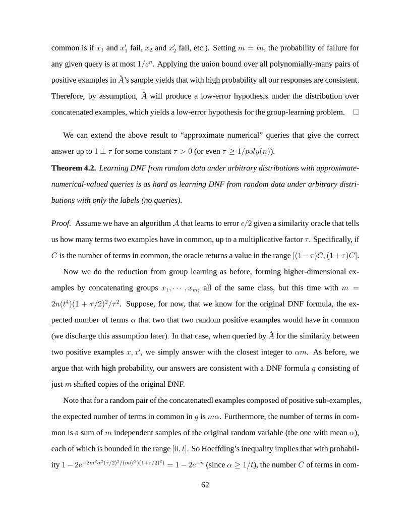
common is ifx1 andx′1 fail, x2 andx′2 fail, etc.). Settingm = tn, the probability of failure for
any given query is at most1/en. Applying the union bound over all polynomially-many pairsof
positive examples inA’s sample yields that with high probability all our responses are consistent.
Therefore, by assumption,A will produce a low-error hypothesis under the distributionover
concatenated examples, which yields a low-error hypothesis for the group-learning problem.
We can extend the above result to “approximate numerical” queries that give the correct
answer up to1± τ for some constantτ > 0 (or evenτ ≥ 1/poly(n)).
Theorem 4.2.Learning DNF from random data under arbitrary distributionswith approximate-
numerical-valued queries is as hard as learning DNF from random data under arbitrary distri-
butions with only the labels (no queries).
Proof. Assume we have an algorithmA that learns to errorǫ/2 given a similarity oracle that tells
us how many terms two examples have in common, up to a multiplicative factorτ . Specifically, if
C is the number of terms in common, the oracle returns a value inthe range[(1−τ)C, (1+τ)C].
Now we do the reduction from group learning as before, forming higher-dimensional ex-
amples by concatenating groupsx1, · · · , xm, all of the same class, but this time withm =
2n(t4)(1 + τ/2)2/τ 2. Suppose, for now, that we know for the original DNF formula,the ex-
pected number of termsα that two that two random positive examples would have in common
(we discharge this assumption later). In that case, when queried byA for the similarity between
two positive examplesx, x′, we simply answer with the closest integer toαm. As before, we
argue that with high probability, our answers are consistent with a DNF formulag consisting of
justm shifted copies of the original DNF.
Note that for a random pair of the concatenatedl examples composed of positive sub-examples,
the expected number of terms in common ing ismα. Furthermore, the number of terms in com-
mon is a sum ofm independent samples of the original random variable (the one with meanα),
each of which is bounded in the range[0, t]. So Hoeffding’s inequality implies that with probabil-
ity 1− 2e−2m2α2(τ/2)2/(m(t2)(1+τ/2)2) = 1− 2e−n (sinceα ≥ 1/t), the numberC of terms in com-
62

mon satisfies|C−mα| ≤ mα(τ/2)/(1+τ/2), which implies(1−τ/2)C ≤ mα ≤ (1+τ/2)C.
Thus, for apoly(n)-sized sample of data points, with high probability, all of the pairs of
positive concatenated examples have the nearest integer tomα within these factors of their true
number of terms in common. It therefore suffices to respond toA’s similarity queries with the
nearest integer tomα.
Now the only trouble is that we do not knowα. So we just try all positive integersi from
1 to mt and then use a validation set to select among the hypotheses produced. That is, we
run A on the constructed data set and respond to all similarity queries with a single valuei,
getting back a classifier for these concatenated examples, and then repeat for eachi. Then we
takeO((1/ǫ) log(mt/δ)) additional higher-dimensional samples (with labels) and choose the
classifier among thesemt returned classifiers, having the smallest number of mistakes there-on.
At least one of thesemt values ofi is the closest integer tomα, so at least one of thesemt
classifiers isǫ/2-good, and our validation set will identify one whose error is at mostǫ. So we
can use this classifier to identify whether a randomm-sized group of examples is composed of
all positives or all negatives, with error rate epsilon: i.e., we can do group learning.
If the algorithm A only has a “high probability” guarantee onsuccess, we can repeat this sev-
eral times with independent data sets, to boost the confidence that there will be a good classifier
among those we choose from at the end, and slightly increase the size of the validation set to
compensate for this larger number of classifiers.
4.3 Learning DNF with General Queries : Positive
4.3.1 Methods
The Neighborhood Method
We refer to the following simple procedure as the “neighborhood method”. Takem = poly(n, 1/ǫ, log(1/δ))
samples. First, among the positive examples, query all pairs (with the binary-valued query) to
63

construct a graph, in which examples are adjacent if they satisfy a term in common. For each
positive example, construct a minimal conjunction consistent with that example and all of its
neighbors (i.e., the consistent conjunction having largest number of literals in it). Next, discard
any of these conjunctions that make mistakes on any negativeexamples. Then sequentially re-
move any conjunctionc1 such that some other remaining conjunctionc2 subsumes it (contains a
subset of the variables). Form a DNF from the remaining conjunctions. Produce this resultant
DNF as the output hypothesis.
Lemma 4.3. Suppose the target DNF hast = poly(n) terms. For an appropriate (t-dependent)
polynomial sample sizem, the neighborhood method will, with probability at least1 − delta,
produce anǫ-accurate DNF if, for each termTi in the target DNF having a probability of satis-
faction at leastǫ/2t, there is at least ap = 1/poly(n, 1/ǫ) probability that a random example
satisfies termTi and no other term (we call such an example a “nice seed” forTi).
Proof. Under these conditions,m = O((1/p) log(t/δ) + (t/ǫ) log(1/ǫδ)) samples suffice to
guarantee eachTi with probability of satisfaction at leastǫ/2t has at least one nice seed, with
probability at least1− δ/2.
In the second phase, we remove any conjunction inconsistentwith the negative examples. The
conjunctions guarnateed by the above argument survive thispruning due to their minimality, and
the fact that they are learned from a set of examples that actually are consistent with some term
in the target DNF (due to the nice seed). The final pruning step, which removes any redundancies
in the set of conjunctions, leaves at mostt conjunctions.
The terms that do not have nice seeds compose at mostǫ/2 total probability mass, andm is
large enough so that with probability at least1− δ/4, at most anǫ/4-fraction of the data satisfy
these terms. Thus, since the result of the neighborhood method is a DNF formula with at most
t terms, which correctly labels a1 − ǫ/2 fraction of them examples, the standard PAC bounds
imply that with probability at least1 − δ/4, the resulting DNF has error rate at mostǫ. A union
bound over the above events implies this holds with probability at least1− δ.
64

The Common Profile Approach
In the case of numerical queries, we have some additional flexibility in designing a method. In
this context, we refer to the following procedure as the “common profiles approach”.
Consider a sample ofm = poly(n, 1/ǫ, log(1/δ)) random labeled examples, and for each
pair of positive examplesx, y, we request the numberK(x, y) of terms they satisfy in common;
we additionally requestK(x, x) for each positive examplex. For each positive examplex, we
identify the setS of examplesy such that the numerical value ofK(x, y) is equalK(x, x). So
these points satisfy at least all the termsx satisfies. For each such setS, we learn a minimal
conjunction consistent with these examples. Then for each of these conjunctions, if it is a spe-
cialization of some other one of the conjunctions, we discard it. Then we form our hypothesis
DNF with the remaining conjunctions as the terms.
For any examplex, relative to a particular target DNF, we refer to the “profile” of x as the set
of termsTi in the target DNF satisfied byx.
Lemma 4.4. If the target DNF has at mostp = poly(n) possibel profiles, then the common
profile approach, with an appropriate (p-dependent) sample sizem, will with probability at least
1− δ, produce a DNF having error rate at mostǫ.
Proof. Note that this procedure produces a DNF that correctly labels the entire data set, since
K(x, y) = K(x, x) impliesx andy have the same profiles, so that in particular the setS has some
term in common to all the examples. If there are only apoly(n) number of possible profiles,
then the above will only produce at most as many distinct terms in its hypothesis DNF, so that a
sufficiently largepoly(n)-sized data set will be sufficient to guarantee good generalization error.
Specifically,m = O((pn/ǫ) log(1/ǫδ)) examples are enough to guarantee with probability at
least1− δ, any DNF consistent with the data having at mostp terms will have error rate at most
ǫ, so this is sufficient for the common profile approach.
65

4.3.2 Positive Results
Theorem 4.5.With numerical-valued queries, we can properly learn any DNF havingO(log(n))
relevant variables, under arbitrary distributions.
Proof. These targets havepoly(n) possible profiles, so the common profiles approach will be
successful.
Theorem 4.6. If the target DNF has onlyO(log(n)) terms, then we can efficiently properly learn
from random data under any distribution using numerical-valued queries.
Proof. There are onlypoly(n) number of possible profiles, so the “common profiles” approach
will work.
The above result is interesting particularly because proper learning (even for 2-term DNF) is
known to be hard from labeled data alone.
Theorem 4.7. If the target DNF hast = poly(n) terms, and is such that any example can satisfy
at mostO(1) terms, then we can efficiently properly learn from random datausing numerical-
valued queries.
Proof. There are at mostpoly(t) = poly(n) possible profiles, so the “common profiles” ap-
proach will work.
Corollary 4.8. We can properly learn anyk-term DNF with numerical-valued queries, wherek
is constant.
Proof. This follows from either Theorem 4.6 or Theorem 4.7.
Corollary 4.9. If the DNF is such that any example can satisfy at most1 term (a so-called
“disjoint” DNF), then we can efficiently properly learn from random data using binary-valued
queries.
Proof. A numerical query whose value can be at most1 is just a binary query anyway.
66

In particular, Decision Trees can be thought of as a DNF whereeach example satisfies at
most1 term.
Lemma 4.10. If it happens that the target DNF is parsimonious (no redundant terms) for some
randomΩ((tn/ǫ) log(1/ǫ) + (1/ǫ) log(1/δ))-sized data set (for any distribution), then we can
efficiently produce a DNF consistent with it having at mostt terms using binary-valued queries.
Proof. (Sketch) Parsimonious, in this case, means that we cannot remove any terms without
changing some labels. But this means that every term has some example that satisfies only that
term (i.e., a nice seed). So as described in the proof of Lemma4.3 above, the “neighborhood
method,” produces a DNF with terms for the neighborhoods of each of these nice seeds, which
in the parsimonious case, covers all of the positive examples.
Theorem 4.11.We can properly learn 2-term DNF with binary queries.
Proof. TakeO((n/ǫ) log(1/ǫ) + (1/ǫ) log(1/δ)) random labeled examples and make the binary
query for all pairs of positive examples. First, find a minimal conjunction consistent with all
of the positive examples; if this conjunction does not misclassify any negative examples, return
it. By classic PAC bounds, a conjunction consistent with thismany random labeled examples
will, with probabiliy at least1 − δ, have error rate at mostǫ. Otherwise, if this conjunction
misclassifies some negatives, then we are assured the targetDNF is parsimonious for this data
set, and thus Lemma 4.10 guarantees we can efficiently identify a 2-term DNF consistent with it
using the binary-valued queries. Again, the classic PAC bounds imply the sample size is large
enough to, with probability at least1 − δ, guarantee that any consistent2-term DNF has error
rate at mostǫ.
Theorem 4.11 gives a concrete result where using this type ofquery overturns a known hard-
ness result for supervised learning.
Open problem Can this idea be extended to learning 3-term DNF or higher, still using only
the binary-valued queries? Or is there a hardness result forproperly learning 3-term DNF with
67

these binary-valued pairwise queries?
4.4 Learning DNF under the Uniform Distribution
In this section, we investigate the problem of learning DNF under a uniform distribution on
0, 1n, using the binary-valued queries.
Definition 4.12. Fix a constantc ∈ (0,∞). We say a termt in the target DNF is “relatively
distinct” if it contains a variablev which occurs in at mostc log(n) other terms. We sayv is a
witness tot being relatively distinct.
Definition 4.13. For a termt in the target DNF, and a variablev in t, we sayv is “sometimes
nonredundant” fort if, given a random example that satisfiest, there is at least anǫ probability
that every term in the target DNF that the example satisfies also containsv.
Theorem 4.14.Suppose no term in the target DNF is logically entailed from any other term
in the target DNF, every termt is relatively distinct, and that some variablev that is a witness
to t being relatively distinct is sometimes nonredundant fort. Then we can properly learn any
monotone DNF of this type under a uniform distribution on0, 1n with binary pairwise queries.
Proof. By Lemma 4.3, it suffices to show that every term having at leastǫ/(2T ) probability of
being satisfied will, with high probability, have some example satisfying only that term, given a
polynomial-sized data set.
Consider a given termt in the target DNF, and choose thev that witnesses relative distinctness
which is sometimes nonredundant. Note that every other termin the target DNF contains some
variable not present int, and in particular this is true for the (at most)c log(n) terms containing
v. So under the conditional distribution given thatt is satisfied and thatv is nonredundant, with
probability at least2−c log(n) = n−c, none of these other terms containingv are satisfied, so thatt
is the only term satisfied. Thus, sincet has probability at leastǫ/(2T ) of being satisfied, andv has
probability at leastǫ of being nonredundant given thatt is satisfied, we have that with probability
68

at least(ǫ2/T )n−c, a random example satisfiest and no other terms in the target DNF.
Since this is the case for all terms in the target, a sample of sizeO((T/ǫ2)nc log(T/δ)) guar-
antees every term has some example satisfying only that term, with probability at least1−δ.
We can also consider the class of DNF function having only a small number of relevant
variables. In this context, it is interesting to observe that if the ith variable is irrelevant, then
P (K(x, y) = 1 andxi 6= yi) = P (K(x, y) = 1 andxi = yi), wherex andy are independent
uniformly-distributed samples, andK(x, y) = 1 iff x andy are positive examples that satisfy at
least one term in common. However, as the following lemma shows, this is not true for relevant
variables.
Lemma 4.15.For x andy independent uniformly-distributed samples, if the targetfunction has
r relevant variables, and theith variable is relevant in the target function, thenP (K(x, y) =
1 andxi = yi)− P (K(x, y) = 1 andxi 6= yi) ≥ (1/4)r.
Proof. For each pair(x, y) with xi 6= yi, there is a unique corresponding pair(x′, y) with x′j = xj
for j 6= i, andx′i = yi. LetMi be the number ofx, y pairs withxi 6= yi andK(x, y) = 1. Then
note that for everyx, y pair with xi 6= yi andK(x, y) = 1, we also haveK(x′, y) = 1, since
whatever termx and y satisfy in common cannot contain variablei anyway, so flipping that
feature inx does not change whetherx andy share a term or not. In particular, this implies
the number ofx, y pairs withxi = yi andK(x, y) = 1 is at leastMi. However, we can also
argue it is strictly larger, as follows. By definition of “relevant”, each of the2r settings of the
relevant variables corresponds to an equivalence class of feature vectors, all of which have the
same label, and if that label is positive, then all of which have the same profile. Since variablei
is relevant, at least one of the2r settings of the relevant variables yields an equivalence class of
positive examples whose profile contains only terms with variable i in them (these are positive
examples such that flipping variablei makes them negative). The probability that bothx andy
(chosen at random) are in this equivalence class is(1/4)r. Note that for the(x, y) pairs of this
type, we haveK(x, y) = 1; however, if we flip featurexi, thenx would become negative, and
69

henceK(x, y) would no longer be1; this means this(x, y) pair is not included among thoseMi
pairs constructed above by flippingxi starting from some(x, y) with xi 6= yi andK(x, y) = 1.
SoP (K(x, y) = 1 andxi = yi)−P (K(x, y) = 1 andxi 6= yi) = (Mi/4n+(1/4)r)−Mi/4
n =
(1/4)r.
Theorem 4.16.Under the uniform distribution, with binary pairwise queries, we can properly
learn any DNF havingO(log(n)) relevant variables.
Proof. We can use the property in Lemma 4.15 to design an algorithm asfollows. For eachi,
sampleΩ(8r log(n/δ)) random pairs(x, y), and evaluateK(x, y) for each pair. Then calculate
the difference of empirical probabilities (fraction of pairs (x, y) for which K(x, y) = 1 and
xi = yi minus fraction of pairs(x, y) for whichK(x, y) = 1 andxi 6= yi). If this difference
is > (1/2)(1/4)r, decide variablei is relevant, and otherwise decide variablei is irrelevant.
By Hoeffding and union bounds, with probability1 − δ/2, this will find exactly ther relevant
variables. Now enumerate all2r = poly(n) possible conjunctions that can be formed from
using all of theser relevant variables. Considering this as a2r-dimensional feature space, take
Ω((2r/ǫ)log(1/δ)) random labeled data points and learn a disjunction over this2r-dimensional
feature space; since the VC dimension of this set of disjunctions is2r, the usual PAC analysis
implies this will learn anǫ-good disjunction with probability1 − δ/2. A union bound implies
both stages (finding variables and learning the disjunction) will succeed with probability at least
1− δ.
An alternative approach to the second stage in the proof would be to takeΩ(2r log(2r/δ))
random samples, so that with probability at least1−δ/2, we have at least one data point satisfying
each of the2r possible conjunctions on the relevant variables; then for each of the conjunctions,
we check the label of the example that satisfies it, and if thatlabel is positive, we include that
conjunction as a term in our DNF, and otherwise we do not include it. This has the property that,
altogether, with probability1− δ, we construct a DNF that has error ratezero.
70

Another family of DNF studied in the literature are those with a sublinear number of terms.
Specifically, [Servedio, 2004] proved that the class of2O(√logn)-termmonotoneDNF are learn-
able under the uniform distribution from labeled data alone. As the following theorem states,
we can extend this result to include general2O(√logn)-term DNF (including non-monotone) given
access to our binary pairwise queries.
Theorem 4.17.Under the uniform distribution, with binary pairwise queries, we can learn any
2O(√log n)-term DNF (supposingǫ to be a constant).
First, we review some known results from [Servedio, 2004]. For any functiong : 0, 1n →
−1,+1, define thegi,1 andgi,0 functions by the property that anyx with xi = 1 hasgi,1(x) =
g(x), andgi,0(x) = g(y), whereyj = xj for j 6= i andyi = 0. Then define the influence
functionIi(g) = P (gi,0(x) 6= gi,1(x)). [Servedio, 2004] developed a procedure,FindVariable,
which uses apoly(n, 1/γ, log(1/η)) number of random labeled samples, labeled according to
any monotone DNFg having at mostt terms, and with probability1 − η, returns a setS of
variables (indices in1, . . . , n) such that everyi /∈ S hasIi(g) ≤ γ and everyi ∈ S has
Ii(g) ≥ γ/2 and theith variable is contained in some term ing with at mostlog 32tnγ
variables in
it.
Furthermore, [Servedio, 2004] showed that, for anyt-term DNFf , if we are provided with
a setSf ⊆ 1, . . . , n such that everyi /∈ Sf hasIi(f) ≤ ǫ/4n, then we can learnf in time
polynomial inn, |Sf |O(log tǫlog 1
ǫ), and log(1/δ). In particular, for|Sf | = O(t log tn
ǫ) and t =
2O(√log n), this is polynomial inn (though not necessarily inǫ). Given the setSf , the learning
procedure simply estimates the Fourier coefficients for small subsets ofSf .
Proof of Theorem 4.17.To prove Theorem 4.17, we consider the following procedure.First
samplem labeled examplesx(1), . . . , x(m) at random. Then, for eachj ≤ m, defineKj(·) =
K(x(j), ·). Now note that, if we defineϕj(y) = (ϕj1(y), . . . , ϕjn(y)) by ϕji(y) = 2I[yi =
x(j)i ]−1, then we can representKj(·) = (K ′
j(ϕj(·))+1)/2, whereK ′j is a monotone DNF (map-
ping into−1,+1); specifically, the terms inK ′j correspond to the terms in the target satisfied
71

by x(j), except none of the literals are negated. We then runFindVariable for each of theseK ′j,
with γ = ǫ/m andη = δ/2m. LetSf denote the union (overj ≤ m) of the returned sets of vari-
ables. It remains only to show thisSf satisfies the requirements for the procedure of [Servedio,
2004], including the size requirement.
Takingm = Ω( ctǫlog t
δ), with probability at least1 − δ/4, every term in the target having
probability at leastǫ/2ct will have at least one of them examples satisfying it. Suppose this
event happens. In particular, this meanserror(maxj Kj) < ǫ/2c. Note that
Ii(f) = P (fi,0(x) 6= fi,1(x)) ≤ 2P (maxjKj(x) 6= f(x)) + P ((max
jKj)i,0(x) 6= (max
jKj)i,1(x))
< ǫ/c+∑
j
P ((K ′j)i,0(x) 6= (K ′
j)i,1(x)) = ǫ/c+∑
j
Ij(K′j).
Thus, by a union bound, with probability1 − δ/2, any variablei /∈ Sf hasIi(f) < ǫ/c +mγ,
and any variablei ∈ Sf appears in a term in someK ′j of size at mostlog 32tn
γ, and therefore
also appear in a corresponding term of this size inf . Suppose this happens. Lettingc = 8n and
γ = ǫ/8nm, we have that anyi /∈ Sf hasIi(f) < ǫ/4n, while anyi ∈ Sf appears in a term of
size at mostlog 256tn2mǫ
= O(log tn log(1/δ)ǫ
). In particular, this implies|Sf | = O(t log tn log(1/δ)ǫ
),
andSf satisfies the requirements of the method of [Servedio, 2004].
Thus, running the procedure from [Servedio, 2004] with confidence parameterδ/4, a union
bound implies the total probability of successfully producing anǫ-good classifier is at least1−δ.
The above process of constructingSf is clearly polynomial-time. Then, ift = 2O(√logn), the
procedure of [Servedio, 2004] runs in time polynomial inn, log(1/δ), and|Sf |O(log(t/ǫ) log(1/ǫ)),
which is polynomial inn andlog(1/δ) (though not necessarily inǫ).
4.5 More Powerful Queries
Theorem 4.18. If we can construct our own feature vectors in addition to getting random data,
then under any distribution we can efficiently properly learnDNF using binary-valued queries.
72

Proof. Suppose we can adaptively construct our own examples. Suppose the target DNF has
T = poly(n) terms. Oracle(x, x′) gives the number of terms thatx andx′ have in common. For
anyx, letx−i be x but with the ith bit flipped. Letx be the negative ofx.
Below is an algorithm.Move(x, x′) movesx′ away fromx by one bit, while trying to main-
tain at least one common term.LearnTerm(x) returns a term in the target function.
0. Move(x, x′)
1. x′′ ← x
2. For i = 1, 2, ..., n s.t.xi = x′i
3. If (Oracle(x, x′′) ≤ Oracle(x, x′−i))
4. x′′ ← x′−i
5. Returnx′′
0. LearnTerm (x)
1. Replicate x to getx′
2. While (Oracle(x, Move(x, x′)) ! = ∅)
3. x′ ← Move(x, x′)
4. LetI ← i : Oracle(x, x′−i) = ∅
5. ReturnxI (i.e. a conjunction with the literals indexed byI, either positive or negative so
thatx satisfies it)
0. LearnDNF
1. Initialize all-negative DNFh
2. TakeM = poly(n)≫ nT random examplesS
73

3. For eachx ∈ S
4. If Oracle(x,x) > 0 (positive example) andh(x) = negative
5. Add term LearnTerm(x) to h
6. Returnh (a DNF with at mostT terms, consistent with all M examples)
When we reachx′ such that we can’t flip any more bits (not already flipped) without making
it so they don’t satisfy any terms in common anymore, then thebits these two have in common
must form a term in the target DNF, so LearnTerm(x) should still find a term in the target DNF.
If we can ask about k-tuples of examples (do they all jointly satisfy a term in common?), we
have the following result:
Theorem 4.19. If we can use query sets of arbitrary sizes (instead of just 2 points), then under
any distribution we can efficiently properly learn DNF using binary-valued queries from random
data.
Proof. We take any set of examples and ask the oracle the number of terms all examples in the
set have in common. Let S be the query set. The idea is to greedily add the examples to S while
keeping some terms in common.
Algorithm :
0. Input : datasetD
1. InitializeS to be an empty set
2. Do
3. Do
4. rmax ← 0
5. For each examplex in the datasetD
6. addx to the setS
74
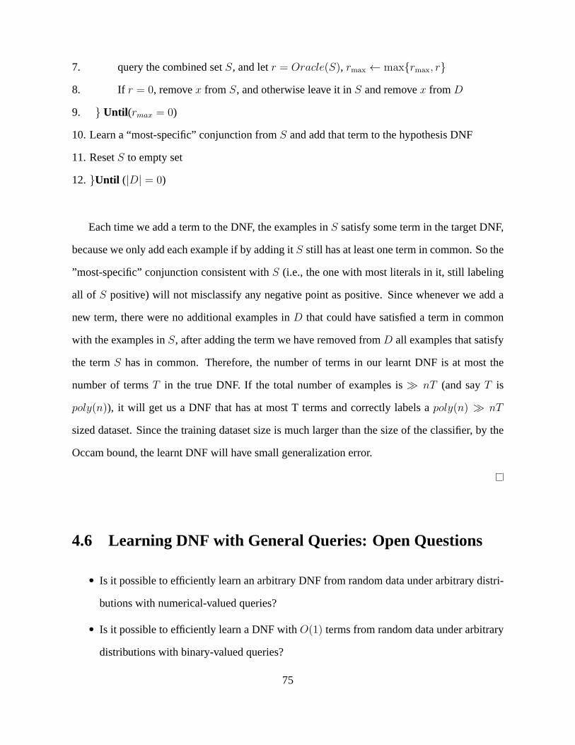
7. query the combined setS, and letr = Oracle(S), rmax ← maxrmax, r
8. If r = 0, removex from S, and otherwise leave it inS and removex fromD
9. Until (rmax = 0)
10. Learn a “most-specific” conjunction fromS and add that term to the hypothesis DNF
11. ResetS to empty set
12. Until (|D| = 0)
Each time we add a term to the DNF, the examples inS satisfy some term in the target DNF,
because we only add each example if by adding itS still has at least one term in common. So the
”most-specific” conjunction consistent withS (i.e., the one with most literals in it, still labeling
all of S positive) will not misclassify any negative point as positive. Since whenever we add a
new term, there were no additional examples inD that could have satisfied a term in common
with the examples inS, after adding the term we have removed fromD all examples that satisfy
the termS has in common. Therefore, the number of terms in our learnt DNF is at most the
number of termsT in the true DNF. If the total number of examples is≫ nT (and sayT is
poly(n)), it will get us a DNF that has at most T terms and correctly labels apoly(n) ≫ nT
sized dataset. Since the training dataset size is much larger than the size of the classifier, by the
Occam bound, the learnt DNF will have small generalization error.
4.6 Learning DNF with General Queries: Open Questions
• Is it possible to efficiently learn an arbitrary DNF from random data under arbitrary distri-
butions with numerical-valued queries?
• Is it possible to efficiently learn a DNF withO(1) terms from random data under arbitrary
distributions with binary-valued queries?
75

• Is it possible to efficiently learn a monotone DNF from randomdata under a uniform
distribution with numerical-valued queries? If so, what about binary-valued queries?
4.7 Generalizations
4.7.1 Learning Unions of Halfspaces
Several of the above results generalize nicely to the more general problem of learning unions of
halfspaces. Specifically, the queries are of the type “do these two examples satisfy a halfspace in
common?” or “how many halfspaces do these two examples satisfy in common?” The general-
ized forms of Theorem 4.19 and Lemma 4.10 follow by the exact same arguments. In each case,
the algorithm finds sets of examples that satisfy some halfspace, such that none of the remaining
examples satisfy that halfspace, so for each such set we simply find a linear separator to separate
those examples from the rest, and take their union to form ourfinal classifier. A sufficiently
large (poly(n,1/ǫ)-sized) set suffices to guarantee this works. It is not so clear how to generalize
Theorem 4.7, since it is not clear how to use the sets of examples with the common profiles to
learn the halfspaces. The generalized version of Theorem 4.6 actually follows from the result
below on learning Voronoi diagrams. The generalized version of Theorem 4.18 is simple, since
it is even known that labeled data plus membership queries are sufficient.
4.7.2 Learning Voronoi with General Queries
Consider the space of Voronoi diagrams (vector quantizers);specifically, the target function is
constant within each cell of the Voronoi diagram, and there are poly(n) such cells for a given
target function. We define a “same cell” query as asking, for apair of examplesx andy, whether
x andy occur in the same cell of the target function. With this type of query, we can efficiently
properly learn Voronoi partitions from random data, under arbitrary distributions. To prove this,
we simply group the examples in a sufficiently large sample into equivalence classes based on
76

these same-cell queries. For each pair of such equivalence classes, we find a linear separator that
separates them. For each test point, we evaluate these linear separators, which thereby associates
the test point with one of the equivalence classes from the training data, and we predict as a label
for that point the label associated with that equivalence class. If we have a sufficiently large
training set, then there is only a small probability the testpoint gets placed into a different set of
points from those in its own cell.
77

Chapter 5
Bayesian Active Learning with Arbitrary
Binary Valued Queries
Abstract
1We investigate the minimum expected number of bits sufficient to encode a random variable X
while still being able to recover an approximation of X with expected distance from X at most
D: that is, the optimal rate at distortion D, in a one-shot coding setting. We find this quantity is
related to the entropy of a Voronoi partition of the values ofX based on a maximal D-packing.
5.1 Introduction
In this work, we study the fundamental complexity of lossy coding. We are particularly interested
in identifying a key quantity that characterizes the expected number of bits (called therate)
required to encode a random variable so that we may recover anapproximation within expected
distanceD (called thedistortion). This topic is a generalization of the well-known analysisof
exact coding by Shannon [Shannon, 1948], where it is known that the optimal expected number
1Joint work with Jaime Carbonell and Steve Hanneke.
78

of bits is precisely characterized by the entropy. There aremany problems in which exact coding
is not practical or not possible, so that lossy coding becomes necessary: particularly for random
variables taking values in uncountably infinite spaces. Thetopic of code lengths for lossy coding
is interesting, both for its direct applications to compression, and also as a general setting in
which to derive lower bounds for specializations of the setting.
There is much existing work on lossy binary codes. In the present work, we are interested
in a “one-shot” analysis of lossy coding [Kieffer, 1993], inwhich we wish to encode a single
random variable, in contrast to the analysis of “asymptotic” source coding [Cover and Thomas,
2006], in which one wishes to simultaneously encode a sequence of random variables. Of par-
ticular relevance to the one-shot coding problem is the analysis of quantizationmethods that
balancedistortion with entropy[Gersho, 1979, Kieffer, 1993, Zador, 1982]. In particular,it is
now well-known that this approach can yield codes that respect a distortion contraint while nearly
minimizing the rate, so that there are near-optimal codes ofthis type [Kieffer, 1993]. Thus, we
have an alternative way to think of the optimal rate, in termsof the rate of the best distortion-
constrained quantization method. While this is interesting, in that it allows us to restrict our focus
in the design of effective coding techniques, it is not as directly helpful if we wish to understand
the behavior of the optimal rate itself. That is, since we do not have an explicit description of the
optimal quantizer, it may often be difficult to study the behavior of its rate under various interest-
ing conditions. There exist classic results lower boundingthe achievable rates, most notably the
famous Shannon lower bound [Shannon, 1959], which under certain restrictions on the source
and the distortion metric, is known to be fairly tight in theasymptoticanalysis of source coding
[Linder and Zamir, 1994]. However, there are few general results explicitly and tightly charac-
terizing the (non-asymptotic) optimal rates for one-shot coding. In particular, to our knowledge,
only a few special-case calculations of the exact value of this optimal rate have been explicitly
carried out, such as vectors of independent Bernoulli or Gaussian random variables [Cover and
Thomas, 2006].
79

Below, we discuss a particular distortion-constrained quantizer, based on a Voronoi partition
induced by a maximal packing. We are interested in theentropyof this quantizer, as a quantity
used to characterize the optimal rate for codes of a given distortion. While it is clear that this
entropy upper bounds the optimal rate, as this is the case foranydistortion-constrained quantizer
[Kieffer, 1993], the novelty of our analysis lies in noting the remarkable fact that the entropy
of any quantizer constructed in this way alsolower boundsthe optimal rate. In particular, this
provides a method for approximately calculating the optimal rate without the need to optimize
over all possible quantizers. Our result is general, in thatit applies to an arbitrary distribution
and an arbitrary distortion measure from a general class of finite-dimensional pseudo-metrics.
This generality is noteworthy, as it leads to interesting applications in statistical learning theory,
which we describe below.
Our analysis is closely related to various notions that arise in the study ofǫ-entropy [Posner
and Rodemich, 1971, Posner, Rodemich, and Rumsey, Jr., 1967], in that we are concerned with
the entropy of a Voronoi partition induced by anǫ-cover. The notion ofǫ-entropy has been
related to the optimal rates for a given distortion (under a slightly different model than studied
here) [Posner and Rodemich, 1971, Posner, Rodemich, and Rumsey, Jr., 1967]. However, there
are some important distinctions, perhaps the most significant of which is that calculating the
ǫ-entropy requires a prohibitive optimization of the entropy over all ǫ-covers; in contrast, the
entropy term in our analysis can be calculated based onany maximal ǫ-packing (which is a
particular type ofǫ-cover). Maximalǫ-packings are easy to construct by greedily adding arbitrary
new elements to the packing that areǫ-far from all elements already added; thus, there is always
a straightforward algorithmic approach to applying our results.
80

5.2 Definitions
We supposeX ∗ is an arbitrary (nonempty) set, equipped with a separable pseudo-metricρ :
X ∗×X ∗ → [0,∞). 2 We supposeX ∗ is accompanied by its Borelσ-algebra induced byρ. There
is additionally a (nonempty, measurable) setX ⊆ X ∗, and we denote byρ = suph1,h2∈X
ρ(h1, h2).
Finally, there is a probability measureπ with π(X ) = 1, and anX -valued random variableX
with distributionπ, referred to here as the “target.” As the distribution is essentially arbitrary, the
results below will hold foranyπ.
A codeis a pair of (measurable) functions(φ, ψ). Theencoder, φ, maps any elementx ∈ X
to a binary sequenceφ(x) ∈ ⋃∞q=00, 1q (the codeword). Thedecoder, ψ, maps any element
c ∈ ⋃∞q=00, 1q to an elementψ(c) ∈ X ∗. For anyq ∈ 0, 1, . . . andc ∈ 0, 1q, let |c| = q
denote thelength of c. A prefix-freecode is any code(φ, ψ) such that nox1, x2 ∈ X have
c(1) = φ(x1) andc(2) = φ(x2) with c(1) 6= c(2) but∀i ≤ |c(1)|, c(2)i = c(1)i : that is, no codeword is
a prefix of another (longer) codeword. LetPF denote the set of all prefix-free binary codes.
Here, we consider a setting where the code(φ, ψ) may belossy, in the sense that for some
values ofx ∈ X , ρ(ψ(φ(x)), x) > 0. Our objective is to design the code to have small expected
loss (in theρ sense), while maintaining as small of an expected codeword length as possible.
Formally, we have the following definition, which essentially describes a notion of optimality
for a lossy code.
Definition 5.1. For anyD > 0, define the optimalrateat distortionD
R(D) = inf
E
[
|φ(X)|]
: (φ, ψ) ∈ PF with
E
[
ρ(
ψ(φ(X)), X)]
≤ D
,
where the random variable in both expectations isX ∼ π.
For our analysis, we will require a notion of dimensionalityfor the pseudo-metricρ. For this,
2The setX ∗ will not play any significant role in the analysis, except to allow for improper learning scenarios to
be a special case of our setting.
81

we adopt the well-knowndoubling dimension[Gupta, Krauthgamer, and Lee, 2003].
Definition 5.2. Define thedoubling dimensiond as the smallest valued such that, for anyx ∈ X ,
and anyǫ > 0, the size of the minimalǫ/2-cover of theǫ-radius ball aroundx is at most2d.
That is, for anyx ∈ X andǫ > 0, there exists a setxi2di=1 of 2d elements ofX such that
x′ ∈ X : ρ(x′, x) ≤ ǫ ⊆2d⋃
i=1
x′ ∈ X : ρ(x′, xi) ≤ ǫ/2.
Note that, as defined here,d is a constant (i.e., has no dependence on thex or ǫ in its defini-
tion). In the analysis below, we will always assumed < ∞. The doubling dimension has been
studied for a variety of spaces, originally by Gupta, Krauthgamer, & Lee [Gupta, Krauthgamer,
and Lee, 2003], and subsequently by many others. In particular, Bshouty, Li, & Long [Bshouty,
Li, and Long, 2009] discuss the doubling dimension of spacesX of binary classifiers, in the
context of statistical learning theory.
5.2.1 Definition of Packing Entropy
Our main result concerns the relation between the optimal rate at a given distortion with the
entropy of a certain quantizer. We now turn to defining this latter quantity.
Definition 5.3. For any D > 0, defineY(D) ⊆ X as a maximalD-packing ofX . That is,
∀x1, x2 ∈ Y(D), ρ(x1, x2) ≥ D, and∀x ∈ X \ Y(D), minx′∈Y(D) ρ(x, x′) < D.
For our purposes, if multiple maximalD-packings are possible, we can choose to define
Y(D) arbitrarily from among these; the results below hold for anysuch choice. Recall that any
maximalD-packing ofX is also aD-cover ofX , since otherwise we would be able to add to
Y(D) thex ∈ X that escapes the cover. That is,∀x ∈ X , ∃y ∈ Y(D) s.t.ρ(x, y) < D.
Next we define a complexity measure, a type of entropy, which serves as our primary quantity
of interest in the analysis ofR(D). It is specified in terms of a partition induced byY(D), defined
as follows.
82

Definition 5.4. For anyD > 0, define
Q(D) =
x ∈ X : z = argminy∈Y(D)
ρ(x, y)
: z ∈ Y(D)
,
where we break ties in theargmin arbitrarily but consistently (e.g., based on a predefined pref-
erence ordering ofY(D)).
Definition 5.5. For any finite (or countable) partitionS ofX into measurable regions (subsets),
define theentropyof S
H(S) = −∑
S∈Sπ(S) log2 π(S).
In particular, we will be interested in the quantityH(Q(D)) in the analysis below.
5.3 Main Result
Our main result can be summarized as follows. Note that, since we took the distributionπ to be
arbitrary in the above definitions, this result holds foranygivenπ.
Theorem 5.6. If d <∞ and ρ <∞, then there is a constantc = O(d) such that∀D ∈ (0, ρ/2),
H (Q (D log2(ρ/D)))− c ≤ R(D) ≤ H (Q (D)) + 1.
It should not be surprising that entropy terms play a key rolein this result, as the entropy is
essential to the analysis of exact coding [Shannon, 1948]. Furthermore,R(D) is tightly charac-
terized by the minimum achievable entropy among all quantizers of distortion at mostD [Kieffer,
1993]. The interesting aspect of Theorem 5.6 is that we can explicitly describe a particular quan-
tizer with near-optimal rate, and its entropy can be explicitly calculated for a variety of scenarios
(X , ρ, π). As for the behavior ofR(D) within the range between the upper and lower bounds
of Theorem 5.6, we should expect the upper bound to be tight when high-probability subsets of
the regions inQ(D) are point-wise well-separated, whileR(D) may be much smaller (perhaps
closer to the lower bound) when this is violated to a large degree, for reasons described in the
proof below.
83

20 40 60 80 1001D
5
10
15
HHPHDLL
BetaH2,5L
Χ2H1L
NH0,1L
Figure 5.1: Plots ofH(Q(D)) as a function of1/D, for various distributionsπ onX = R.
Although this result is stated for bounded psuedo-metricsρ, it also has implications for un-
boundedρ. In particular, the proof of the upper bound holds as-is for unboundedρ. Furthermore,
we can always use this lower bound to construct a lower bound for unboundedρ, simply restrict-
ing to a bounded subset ofX with constant probability and calculating the lower bound for that
region. For instance, to get a lower bound forπ as a Gaussian distribution onR, we might note
thatπ([−1/2, 1/2]) times the expected loss under theconditionalπ(·|[−1/2, 1/2]) lower bounds
the total expected loss. Thus, calculating the lower bound of Theorem 5.6 under the conditional
π(·|[−1/2, 1/2]) while replacingD with D/π([−1/2, 1/2]) provides a lower bound onR(D).
To get a feel for the behavior ofH (Q (D)), we have plotted it as a function of1/D for several
distributions, in Figure 5.1.
5.4 Proof of Theorem 5.6
We first state a lemma, due to Gupta, Krauthgamer, & Lee [Gupta, Krauthgamer, and Lee, 2003],
which will be useful in the proof of Theorem 5.6.
Lemma 5.7. [Gupta, Krauthgamer, and Lee, 2003] For anyγ ∈ (0,∞), δ ∈ [γ,∞), andx ∈ X ,
|x′ ∈ Y(γ) : ρ(x′, x) ≤ δ| ≤(
4δ
γ
)d
.
In particular, note that this lemma implies that the minimumof ρ(x, y) over y ∈ Y(D) is
alwaysachievedin Definition 5.4, so thatQ(D) is well-defined.
84

We are now ready for the proof of Theorem 5.6.
Proof of Theorem 5.6.Throughout the proof, we will consider a set-valued random quantity
QD(X) with value equal to the set inQ(D) containingX, and a correspondingX -valued random
quantityYD(X) with value equal the sole point inQD(X) ∩ Y(D): that is, the target’s nearest
representative in theD-packing. Note that, by Lemma 5.7,|Y(D)| < ∞ for all D ∈ (0, 1). We
will also adopt the usual notation for entropy (e.g.,H(QD(X))) and conditional entropy (e.g.,
H(QD(X)|Z)) [Cover and Thomas, 2006], both in base 2.
To establish the upper bound, we simply takeφ as the Huffman code for the random quantity
QD(X) [Cover and Thomas, 2006, Huffman, 1952]. It is well-known that the expected length
of a Huffman code forQD(X) is at mostH(QD(X)) + 1 (in fact, is equalH(QD(X)) when
the probabilities are powers of2) [Cover and Thomas, 2006, Huffman, 1952], and each possible
value ofQD(X) is assigned a unique codeword so that we can perfectly recoverQD(X) (and thus
alsoYD(X)) based onφ(X). In particular, defineψ(φ(X)) = YD(X). Finally, recall that any
maximalD-packing is also aD-cover. Thus, since every element of the setQD(X) hasYD(X) as
its closest representative inY(D), we must haveρ(X,ψ(φ(X))) = ρ(X, YD(X)) < D. In fact,
as this proof never relies onρ <∞, this establishes the upper bound even in the caseρ =∞.
The proof of the lower bound is somewhat more involved, though the overall idea is simple
enough. Essentially, the lower bound would be straightforward if the regions ofQ(D log2(ρ/D))
were separated by some distance, since we could make an argument based on Fano’s inequality
to say that since anyX = ψ(φ(X)) is “close” to at most one region, the expected distance
from X is at least as large as half this inter-region distance timesa quantity proportional to the
conditional entropyH(QD(X)|φ(X)), so thatH(φ(X)) can be related toH(QD(X)).
However, the general case is not always so simple, as the regions can generally be quite close
to each other (even adjacent), so that it is possible forX to be close to multiple regions. Thus, the
proof will first “color” the regions ofQ(D log2(ρ/D)) in a way that guarantees no two regions of
the same color are within distanceD log2(ρ/D) of each other. Then we apply the above simple
85

argument for each color separately (i.e., lower bounding the expected distance fromX under the
conditional given the color ofQD log2(ρ/D)(X) by a function of the conditional entropy under the
conditional), and average over the colors to get a global lower bound. The details follow.
Fix anyD ∈ (0, ρ/2), and for brevity letα = D log2(ρ/D). We suppose(φ, ψ) is some
prefix-free binary code.
Define a functionK : Q(α)→ N such that∀Q1, Q2 ∈ Q(α),
K(Q1) = K(Q2) =⇒ infx1∈Q1,x2∈Q2
ρ(x1, x2) ≥ α, (5.1)
and supposeK has minimumH(K(Qα(X))) subject to (5.1). We will refer toK(Q) as thecolor
of Q.
Now we are ready to bound the expected distance fromX. Let X = ψ(φ(X)), and let
Qα(X;K) denote the setQ ∈ Q(α) havingK(Q) = K with smallestinfx∈Q ρ(x, X) (breaking
ties arbitrarily). We know
E[ρ(X,X)] = E
[
E[ρ(X,X)|K(Qα(X))]]
. (5.2)
Furthermore, by (5.1) and a triangle inequality, we know noX can be closer thanα/2 to more
than oneQ ∈ Q(α) of a given color. Therefore,
E[ρ(X,X)|K(Qα(X))]
≥ α
2P(Qα(X;K(Qα(X))) 6= Qα(X)|K(Qα(X))). (5.3)
By Fano’s inequality, we have
E
[
P(Qα(X;K(Qα(X))) 6= Qα(X)|K(Qα(X)))]
≥ H(Qα(X)|φ(X),K(Qα(X)))− 1
log2 |Y(α)|. (5.4)
It is generally true that, for a prefix-free binary codeφ(X), φ(X) is a lossless prefix-free
binary code for itself (i.e., with the identity decoder), sothat the classic entropy lower bound on
average code length [Cover and Thomas, 2006, Shannon, 1948] impliesH(φ(X)) ≤ E[|φ(X)|].
86

Also, recalling thatY(α) is maximal, and therefore also anα-cover, we have that anyQ1, Q2 ∈
Q(α) with infx1∈Q1,x2∈Q2
ρ(x1, x2) ≤ α haveρ(Yα(x1), Yα(x2)) ≤ 3α (by a triangle inequality).
Therefore, Lemma 5.7 implies that, for any givenQ1 ∈ Q(α), there are at most12d setsQ2 ∈
Q(α) with infx1∈Q1,x2∈Q2
ρ(x1, x2) ≤ α. We therefore know there exists a functionK′ : Q(α)→ N
satisfying (5.1) such thatmaxQ∈Q(α)
K′(Q) ≤ 12d (i.e., we need at most12d colors to satisfy (5.1)).
That is, if we consider coloring the setsQ ∈ Q(α) sequentially, for any givenQ1 not yet colored,
there are< 12d setsQ2 ∈ Q(α) \ Q1 within α of it, so there must exist a color among
1, . . . , 12d not used by any of them, and we can choose that forK′(Q1). In particular, by our
choice ofK to minimizeH(K(Qα(X))) subject to (5.1), this implies
H(K(Qα(X))) ≤ H(K′(Qα(X))) ≤ log2(12d) ≤ 4d.
Thus,
H(Qα(X)|φ(X),K(Qα(X)))
= H(Qα(X), φ(X),K(Qα(X)))
−H(φ(X))−H(K(Qα(X))|φ(X))
≥ H(Qα(X))−H(φ(X))−H(K(Qα(X)))
≥ H(Qα(X))− E [|φ(X)|]− 4d
= H(Q(α))− E [|φ(X)|]− 4d. (5.5)
Thus, combining (5.2), (5.3), (5.4), and (5.5), we have
E[ρ(X,X)] ≥ α
2
H(Q(α))− E [|φ(X)|]− 4d− 1
log2 |Y(α)|
≥ α
2
H(Q(α))− E [|φ(X)|]− 4d− 1
d log2(4ρ/α),
where the last inequality follows from Lemma 5.7.
Thus, for any code with
E [|φ(X)|] < H(Q(α))− 4d− 1− 2dlog2(4ρ/D)
log2(ρ/D),
87

we haveE[ρ(X,X)] > D, which implies
R(D) ≥ H(Q(α))− 4d− 1− 2dlog2(4ρ/D)
log2(ρ/D).
Sincelog2(4ρ/D)/ log2(ρ/D) ≤ 3, we have
R(D) ≥ H(Q(α))−O(d).
5.5 Application to Bayesian Active Learning
As an example, in the special case of the problem of learning abinary classifier, as studied by
[Haussler, Kearns, and Schapire, 1994a] and [Freund, Seung, Shamir, and Tishby, 1997],X ∗ is
the set of all measurable classifiersh : Z → −1,+1, X is called the “concept space,”X is
called the “target function,” andρ(X1, X2) = P(X1(Z) 6= X2(Z)), whereZ is someZ-valued
random variable. In particular,ρ(X1, X) is called the “error rate” ofX1.
We may then discuss alearning protocolbased on binary-valued queries. That is, we sup-
pose some learning machine is able to pose yes/no questions to an oracle, and based on the
responses it proposes ahypothesisX. We may ask how many such yes/no questions must the
learning machine pose (in expectation) before being able toproduce a hypothesisX ∈ X ∗ with
E[ρ(X,X)] ≤ ǫ, known as thequery complexity.
If the learning machine is allowed to posearbitrary binary-valued queries, then this setting is
precisely a special case of the general lossy coding problemstudied above. That is, any learning
machine that asks a sequence of yes/no questions before terminating and returning someX ∈ X ∗
can be thought of as a binary decision tree (no = left, yes = right), with the returnX values stored
in the leaf nodes. Transforming each root-to-leaf path in the decision tree into a codeword (left
= 0, right = 1), we see that the algorithm corresponds to a prefix-free binary code. Conversely,
given any prefix-free binary code, we can construct an algorithm based on sequentially asking
88

queries of the form “what is the first bit in the codewordφ(X) forX?”, “what is the second bit in
the codewordφ(X) forX?”, etc., until we obtain a complete codeword, at which pointwe return
the value that codeword decodes to. From this perspective, the query complexity is precisely
R(ǫ).
This general problem of learning with arbitrary binary-valued queries was studied previously
by Kulkarni, Mitter, & Tsitsiklis [Kulkarni, Mitter, and Tsitsiklis, 1993], in aminimaxanalysis
(studying the worst-case value ofX). In particular, they find that for a given distribution for
Z, the worst-case query complexity is essentially characterized by log |Y(ǫ)|. The techniques
employed are actually far more general than the classifier-learning problem, and actually apply
to any pseudo-metric space. Thus, we can abstractly think oftheir work as a minimax analysis
of lossy coding.
In addition to being quite interesting in their own right, the results of Kulkarni, Mitter, &
Tsitsiklis [Kulkarni, Mitter, and Tsitsiklis, 1993] have played a significant role in the recent
developments in active learning withlabel requestqueries for binary classification [Dasgupta,
2005, Hanneke, 2007a,b], in which the learning machine may only ask questions of the form,
“What is the valueX(z)?” for certain valuesz ∈ Z. Since label requests can be viewed as
a type of binary-valued query, the number of label requests necessary for learning is naturally
lower bounded by the number ofarbitrary binary-valued queries necessary for learning. We
therefore always expect to see some term relating tolog |Y(ǫ)| in any minimax query complexity
results for active learning with label requests (though this factor is typically represented by its
upper bound:∝ V · log(1/ǫ), whereV is the VC dimension).
Similarly to how the work of Kulkarni, Mitter, & Tsitsiklis [Kulkarni, Mitter, and Tsitsiklis,
1993] can be used to argue thatlog |Y(ǫ)| is a lower bound on the minimax query complexity of
active learning with label requests, Theorem 5.6 can be usedto argue thatH(Q(ǫ log2(1/ǫ))) −
O(d) is a lower bound on the query complexity of learning relativeto a given distribution for
X (called aprior, in the language of Bayesian statistics), rather than the worst-case value ofX.
89

Furthermore, as with [Kulkarni, Mitter, and Tsitsiklis, 1993], this lower bound remains valid for
learning with label requests, since label requests are a type of binary-valued query. Thus, we
should expect a term related toH(Q(ǫ)) orH(Q(ǫ log2(1/ǫ))) to appear in any tight analysis of
the query complexity of Bayesian learning with label requests.
5.6 Open Problems
In our present context, there are several interesting questions, such as whether thelog(ρ/D) factor
in the entropy argument of the lower bound can be removed, whether the additive constant in the
lower bound might be improved, and in particular whether a similar result might be obtained
without assumingd < ∞ (e.g., in the statistical learning special case, by making aVC class
assumption instead).
90

Chapter 6
The Sample Complexity of Self-Verifying
Bayesian Active Learning
Abstract
1We prove that access to a prior distribution over target functions can dramatically improve the
sample complexity of self-terminating active learning algorithms, so that it is always better than
the known results for prior-dependent passive learning. Inparticular, this is in stark contrast to
the analysis of prior-independent algorithms, where thereare simple known learning problems
for which no self-terminating algorithm can provide this guarantee for all priors.
6.1 Introduction and Background
Active learningis a powerful form of supervised machine learning characterized by interaction
between the learning algorithm and supervisor during the learning process. In this work, we
consider a variant known aspool-basedactive learning, in which a learning algorithm is given
access to a (typically very large) collection of unlabeled examples, and is able to select any of
1Joint work with Jaime Carbonell and Steve Hanneke.
91

those examples, request the supervisor to label it (in agreement with the target concept), then after
receiving the label, selects another example from the pool,etc. This sequential label-requesting
process continues until some halting criterion is reached,at which point the algorithm outputs
a function, and the objective is for this function to closelyapproximate the (unknown) target
concept in the future. The primary motivation behind pool-based active learning is that, often,
unlabeled examples are inexpensive and available in abundance, while annotating those examples
can be costly or time-consuming; as such, we often wish to select only the informative examples
to be labeled, thus reducing information-redundancy to some extent, compared to the baseline of
selecting the examples to be labeled uniformly at random from the pool (passive learning).
There has recently been an explosion of fascinating theoretical results on the advantages of
this type of active learning, compared to passive learning,in terms of the number of labels re-
quired to obtain a prescribed accuracy (called thesample complexity): e.g., [Balcan, Broder, and
Zhang, 2007a, Balcan, Beygelzimer, and Langford, 2009, Balcan, Hanneke, and Vaughan, 2010,
Beygelzimer, Dasgupta, and Langford, 2009, Castro and Nowak,2008, Dasgupta, 2004, 2005,
Dasgupta, Hsu, and Monteleoni, 2007b, Dasgupta, Kalai, andMonteleoni, 2009, Freund, Seung,
Shamir, and Tishby, 1997, Friedman, 2009, Hanneke, 2007a,b, 2009, 2011, Kaariainen, 2006,
Koltchinskii, 2010, Nowak, 2008, Wang, 2009]. In particular, [Balcan, Hanneke, and Vaughan,
2010] show that in noise-free binary classifier learning, for any passive learning algorithm for a
concept space of finite VC dimension, there exists an active learning algorithm with asymptoti-
cally much smaller sample complexity for any nontrivial target concept. In later work, [Hanneke,
2009] strengthens this result by removing a certain strong dependence on the distribution of the
data in the learning algorithm. Thus, it appears there are profound advantages to active learning
compared to passive learning.
However, the ability to rapidly converge to a good classifierusing only a small number of
labels is only one desirable quality of a machine learning method, and there are other qualities
that may also be important in certain scenarios. In particular, the ability toverify the performance
92

of a learning method is often a crucial part of machine learning applications, as (among other
things) it helps us determine whether we have enough data to achieve a desired level of accuracy
with the given method. In passive learning, one common practice for this verification is to hold
out a random sample of labeled examples as avalidation sampleto evaluate the trained classifier
(e.g., to determine when training is complete). It turns outthis technique is not feasible in active
learning, since in order to be really useful as an indicator of whether we have seen enough la-
bels to guarantee the desired accuracy, the number of labeled examples in the random validation
sample would need to be much larger than the number of labels requested by the active learning
algorithm itself, thus (to some extent) canceling the savings obtained by performing active rather
than passive learning. Another common practice in passive learning is to examine the training er-
ror rate of the returned classifier, which can serve as a reasonable indicator of performance (after
adjusting for model complexity). However, again this measure of performance is not necessarily
reasonable for active learning, since the set of examples the algorithm requests the labels of is
typically distributed very differently from the test examples the classifier will be applied to after
training.
This reasoning indicates that performance verification is (at best) a far more subtle issue in
active learning than in passive learning. Indeed, [Balcan, Hanneke, and Vaughan, 2010] note that
although the number of labels required to achieve good accuracy is significantly smaller than
passive learning, it is often the case that the number of labels required toverify that the accuracy
is good is not significantly improved. In particular, this phenomenon can dramatically increase
the sample complexity of active learning algorithms that adaptively determine how many labels
to request before terminating. In short, if we require the algorithm both tolearn an accurate
concept and toknow that its concept is accurate, then the number of labels required by active
learning is often not significantly smaller than the number required by passive learning.
We should note, however, that the above results were proven for a learning scenario in which
the target concept is considered a constant, and no information about the process that generates
93

this concept is known a priori. Alternatively, we can consider a modification of this problem, so
that the target concept can be thought of as a random variable, a sample from a known distribution
(called aprior) over the space of possible concepts. Such a setting has beenstudied in detail
in the context of passive learning for noise-free binary classification. In particular, [Haussler,
Kearns, and Schapire, 1994a] found that for any concept space of finite VC dimensiond, for
any prior and distribution over data points,O(d/ε) random labeled examples are sufficient for
the expected error rate of the Bayes classifier produced underthe posterior distribution to be at
mostε. Furthermore, it is easy to construct learning problems forwhich there is anΩ(1/ε) lower
bound on the number of random labeled examples required to achieve expected error rate at most
ε, by any passive learning algorithm; for instance, the problem of learning threshold classifiers
on [0, 1] under a uniform data distribution and uniform prior is one such scenario.
In the context of active learning (again, with access to the prior), [Freund, Seung, Shamir, and
Tishby, 1997] analyze theQuery by Committeealgorithm, and find that if a certain information
gain quantity for the points requested by the algorithm is lower-bounded by a valueg, then the
algorithm requires onlyO((d/g) log(1/ε)) labels to achieve expected error rate at mostε. In par-
ticular, they show that this is satisfied forconstantg for linear separators under a near-uniform
prior, and a near-uniform data distribution over the unit sphere. This represents a marked im-
provement over the results of [Haussler, Kearns, and Schapire, 1994a] for passive learning, and
since the Query by Committee algorithm is self-verifying, this result is highly relevant to the
present discussion. However, the condition that the information gains be lower-bounded by a
constant is quite restrictive, and many interesting learning problems are precluded by this re-
quirement. Furthermore, there exist learning problems (with finite VC dimension) for which the
Query by Committee algorithm makes an expected number of label requests exceedingΩ(1/ε).
To date, there has not been a general analysis of how the valueof g can behave as a function of
ε, though such an analysis would likely be quite interesting.
In the present paper, we take a more general approach to the question of active learning with
94

access to the prior. We are interested in the broad question of whether access to the prior bridges
the gap between the sample complexity oflearningand the sample complexity of learningwith
verification. Specifically, we ask the following question.
Can a prior-dependent self-terminating active learning algorithm for a concept class of finite
VC dimension always achieve expected error rate at mostε usingo(1/ε) label requests?
After some basic definitions in Section 6.2, we begin in Section 6.4 with a concrete example,
namely interval classifiers under a uniform data density butarbitrary prior, to illustrate the general
idea, and convey some of the intuition as to why one might expect a positive answer to this
question. In Section 6.5, we present a general proof that theanswer isalways“yes.” As the
known results for the sample complexity of passive learningwith access to the prior are typically
∝ 1/ε [Haussler, Kearns, and Schapire, 1994a], and this is sometimes tight, this represents
an improvement over passive learning. The proof is simple and accessible, yet represents an
important step in understanding the problem of self-termination in active learning algorithms, and
the general issue of the complexity of verification. Also, asthis is a result that doesnotgenerally
hold for prior-independent algorithms (even for their “average-case” behavior induced by the
prior) for certain concept spaces, this also represents a significant step toward understanding the
inherent value of having access to the prior.
6.2 Definitions and Preliminaries
First, we introduce some notation and formal definitions. Wedenote byX the instance space,
representing the range of the unlabeled data points, and we suppose a distributionD on X ,
which we will refer to as thedata distribution. We also suppose the existence of a sequence
X1, X2, . . . of i.i.d. random variables, each with distributionD, referred to as the unlabeled
data sequence. Though one could potentially analyze the achievable performance as a function
of the number of unlabeled points made available to the learning algorithm (cf. [Dasgupta,
2005]), for simplicity in the present work, we will suppose this unlabeled sequence is essentially
95

inexhaustible, corresponding to the practical fact that unlabeled data are typically available in
abundance as they are often relatively inexpensive to obtain. Additionally, there is a setC of
measurable classifiersh : X → −1,+1, referred to as theconcept space. We denote byd
the VC dimension ofC, and in our present context we will restrict ourselves to spacesC with
d < ∞, referred to as aVC class. We also have a probability distributionπ, called theprior,
overC, and a random variableh∗ ∼ π, called thetarget function; we supposeh∗ is independent
from the data sequenceX1, X2, . . .. We adopt the usual notation for conditional expectations
and probabilities [Ash and Doleans-Dade, 2000]; for instance,E[A|B] can be thought of as an
expectation of the valueA, under the conditional distribution ofA given the value ofB (which
itself is random), and thus the value ofE[A|B] is essentially determined by the value ofB. For
any measurableh : X → −1,+1, define theerror rate er(h) = D(x : h(x) 6= h∗(x)).
So far, this setup is essentially identical to that of [Freund, Seung, Shamir, and Tishby, 1997,
Haussler, Kearns, and Schapire, 1994a].
The protocol in active learning is the following. An active learning algorithmA is given as
input the priorπ, the data distributionD (though see Section 6.6), and a valueε ∈ (0, 1]. It
also (implicitly) depends on the data sequenceX1, X2, . . ., and has an indirect dependence on
the target functionh∗ via the following type of interaction. The algorithm may inspect the values
Xi for any initial segment of the data sequence, select an indexi ∈ N to “request” the label of;
after selecting such an index, the algorithm receives the value h∗(Xi). The algorithm may then
select another index, request the label, receive the value of h∗ on that point, etc. This happens
for a number of rounds,N(A, h∗, ε,D, π), before eventually the algorithm halts and returns a
classifierh. An algorithm is said to becorrect if E
[
er(
h)]
≤ ε for every(ε,D, π); that is,
given direct access to the prior and the data distribution, and given a specified valueε, a correct
algorithm must be guaranteed to have expected error rate at mostε. Define theexpected sample
complexityof A for (X ,C,D, π) to be the functionSC(ε,D, π) = E[N(A, h∗, ε,D, π)]: the
expected number of label requests the algorithm makes.
96
6.3 Prior-Independent Learning Algorithms
One may initially wonder whether we could achieve thiso(1/ε) result merely by calculating
the expected sample complexity of some prior-independent method, thus precluding the need
for novel algorithms. Formally, we say an algorithmA is prior-independent if the conditional
distribution of the queries and return value ofA(ε,D, π) given(X1, X(X1)), (X2, X(X2)), . . .
is functionally independent ofπ. Indeed, for someC andD, it is known that thereare prior-
independent active learning algorithmsA that haveE[N(A, X, ε,D, π)|X] = o(1/ε) (always);
for instance, threshold classifiers have this property under anyD, homogeneous linear separators
have this property under a uniformD on the unit sphere ink dimensions, and intervals with
positive width onX = [0, 1] have this property underD = Uniform([0, 1]) (see e.g., [Dasgupta,
2005]). It is straightforward to show that any suchA will also haveSC(A, ε,D, π) = o(1/ε)
for everyπ. In particular, the law of total expectation and the dominated convergence theorem
imply
limε→0
εSC(A, ε,D, π) = limε→0
εE[E[N(A, X, ε,D, π)|X]]
= E
[
limε→0
εE[N(A, X, ε,D, π)|X]]
= 0.
In these cases, we can think ofSC as a kind ofaverage-caseanalysis of these algorithms. How-
ever, as we discuss next, there are also manyC andD for which there isno prior-independent
algorithm achievingo(1/ε) sample complexity forall priors. Thus, any general result ono(1/ε)
expected sample complexity forπ-dependent algorithms would indicate that there is a real ad-
vantage to having access to the prior, beyond the apparentsmoothingeffects of an average-case
analysis.
As an example of a problem where no prior-independent self-verifying algorithm can achieve
o(1/ε) sample complexity, considerX = [0, 1],D = Uniform([0, 1]), andC as the concept space
of interval classifiers: C = I±(a,b) : 0 ≤ a ≤ b ≤ 1, whereI±(a,b)(x) = +1 if x ∈ (a, b) and
−1 otherwise. Note that because we allowa = b, there is a classifierh− ∈ C labeling all ofX
97

negative. For0 ≤ a ≤ b ≤ 1, let π(a,b) denote the prior withπ(a,b)(I±(a,b)) = 1. We now show
any correct prior-independent algorithm hasΩ(1/ε) sample complexity forπ(0,0), following a
technique of [Balcan, Hanneke, and Vaughan, 2010]. Consider any ε ∈ (0, 1/144) and any
prior-independent active learning algorithmA with SC(A, ε,D, π(0,0)) < s = 1144ε
. Then define
Hε =
(12iε, 12(i+ 1)ε) : i ∈
0, 1, . . . ,⌊
1−12ε12ε
⌋
. Let h(a,b) denote the classifier returned
by A(ε,D, ·) when queries are answered withX = I±(a,b), for 0 ≤ a ≤ b ≤ 1, and letR(a,b)
denote the set of examples(x, y) for whichA(ε,D, ·) requests labels (including theiry = X(x)
labels). The point of this construction is that, with such a small number of queries, for many
of the (a, b) ∈ Hε, the algorithm must behave identically forX = I±(a,b) as forX = I
±(0,0) (i.e.,
R(a,b) = R(0,0), and henceh(a,b) = h(0,0)). Theseπ(a,b) priors will then witness the fact thatA is
not a correct self-verifying algorithm. Formally,
max(a,b)∈Hε
E
[
D(x : h(a,b)(x) 6= I±(a,b)(x))
]
≥ 1
|Hε|∑
(a,b)∈Hε
E
[
D(x : h(a,b)(x) 6= I±(a,b)(x))
]
≥ 1
|Hε|E
∑
(a,b)∈Hε:R(a,b)=R(0,0)
D(x : h(a,b)(x) 6= I±(a,b)(x))
≥ 1
|Hε|E
∑
(a,b)∈Hε:R(a,b)=R(0,0)
(
12ε−minD(x : h(a,b)(x) 6= −1), 12ε)
. (6.1)
Since the summation in (6.1) is restricted to(a, b) with R(a,b) = R(0,0), these(a, b) must also
haveh(a,b) = h(0,0), so that (6.1) equals
1
|Hε|E
∑
(a,b)∈Hε:R(a,b)=R(0,0)
(
12ε−minD(x : h(0,0)(x) 6= −1), 12ε)
. (6.2)
Furthermore, for a givenX1, X2, . . . sequence, the only(a, b) ∈ Hε with R(a,b) 6= R(0,0) are
those for which some(x,−1) ∈ R(0,0) hasx ∈ (a, b); since the(a, b) ∈ Hε are disjoint, the
98

above summation has at least|Hε| − |R(0,0)| elements in it. Thus, (6.2) is at least
E
[( |Hε| −min|R(0,0)|, |Hε||Hε|
)
(
12ε−minD(x : h(0,0)(x) 6= −1), 12ε)
]
≥ E
[
I[
|R(0,0)| ≤ 3s]
I
[
D(x : h(0,0)(x) 6= −1) ≤ 6ε]
( |Hε| − 3s
|Hε|
)
(12ε− 6ε)
]
≥ 3εP(
|R(0,0)| ≤ 3s,D(x : h(0,0)(x) 6= −1) ≤ 6ε)
. (6.3)
By Markov’s inequality,
P(
|R(0,0)| > 3s)
≤ E[|R(0,0)|]/(3s) = SC(A, ε,D, π(0,0))/(3s) < 1/3,
andP(
D(x : h(0,0)(x) 6= −1) > 6ε)
≤ E
[
D(x : h(0,0)(x) 6= −1)]
/(6ε), and ifA is a correct
self-verifying algorithm, thenE[
D(x : h(0,0)(x) 6= −1)]
/(6ε) ≤ 1/6. Thus, by a union bound,
(6.3) is at least3ε(1− 1/3− 1/6) = (3/2)ε > ε. Therefore,A cannot be a correct self-verifying
learning algorithm.
6.4 Prior-Dependent Learning: An Example
We begin our exploration ofπ-dependent active learning with a concrete example, namelyinter-
val classifiers under a uniform data density but arbitrary prior, to illustrate how access to the prior
can make a difference in the sample complexity. Specifically, considerX = [0, 1], D uniform
on [0, 1], and the concept spaceC of interval classifiers specified in the previous section. For
each classifierh ∈ C, definew(h) = D(x : h(x) = +1) (the width of the intervalh). Note that
because we allowa = b in the definition ofC, there is a classifierh− ∈ C with w(h−) = 0.
For simplicity, in this example (only) we will suppose the algorithm may request the label
of any point in X , not just those in the sequenceXi; the same ideas can easily be adapted
to the setting where queries are restricted toXi. Consider an active learning algorithm that
sequentially requests the labelsX(x) for pointsx at 1/2, 1/4, 3/4, 1/8, 3/8, 5/8, 7/8, 1/16,
3/16, etc., until (case 1) it encounters an examplex with X(x) = +1 or until (case 2) the set of
99

classifiersV ⊆ C consistent with all observed labels so far satisfiesE[w(X)|V ] ≤ ε (which ever
comes first). In case 2, the algorithm simply halts and returns the constant classifier that always
predicts−1: call it h−; note thater(h−) = w(X). In case 1, the algorithm enters a second phase,
in which it performs a binary search (repeatedly querying the midpoint between the closest two
−1 and+1 points, taking0 and1 as known negative points) to the left and right of the observed
positive point, halting afterlog2(4/ε) label requests on each side; this results in estimates of the
target’s endpoints up to±ε/4, so that returning any classifier among the setV ⊆ C consistent
with these labels results in error rate at mostε; in particular, if h is the classifier inV returned,
thenE[er(h)|V ] ≤ ε.
Denoting this algorithm byA[], andh the classifier it returns, we have
E
[
er(
h)]
= E
[
E
[
er(
h) ∣
∣
∣V]]
≤ ε,
so that the algorithm is definitely correct.
Note that case 2 will definitely be satisfied after at most2ε
label requests, and ifw(X) > ε,
then case 1 will definitely be satisfied after at most2w(X)
label requests, so that the algorithm never
makes more than 2maxw(X),ε label requests before satisfying one of the two cases. Abbreviating
N(X) = N(A[], X, ε,D, π), we have
E [N(X)]
= E
[
N(X)∣
∣
∣w(X) = 0]
P (w(X) = 0)
+ E
[
N(X)∣
∣
∣0 < w(X) ≤ √ε
]
P(
0 < w(X) ≤ √ε)
+ E
[
N(X)∣
∣
∣w(X) >√ε]
P(
w(X) >√ε)
≤ E
[
N(X)∣
∣
∣w(X) = 0]
P (w(X) = 0) +2
εP(
0 < w(X) ≤ √ε)
+2√ε+ 2 log2
4
ε. (6.4)
The third and fourth terms in (6.4) areo(1/ε). SinceP(0 < w(X) ≤ √ε) → 0 asε → 0, the
second term in (6.4) iso(1/ε) as well. IfP(w(X) = 0) = 0, this completes the proof. We focus
the rest of the proof on the first term in (6.4), in the case thatP(w(X) = 0) > 0: i.e., there is
100

nonzero probability that the targetX labels the space all negative. LettingV denote the subset
of C consistent with all requested labels, note that on the eventw(X) = 0, aftern label requests
(for n + 1 a power of2) we havemaxh∈V w(h) ≤ 1/n. Thus, for any valueγ ∈ (0, 1), after at
most 2γ
label requests, on the event thatw(X) = 0,
E
[
w(X)∣
∣
∣V]
≤ E [w(X)I [w(X) ≤ γ]]
π(V )≤ E [w(X)I [w(X) ≤ γ]]
P(w(X) = 0). (6.5)
Now note that, by the dominated convergence theorem,
limγ→0
E
[
w(X)I [w(X) ≤ γ]
γ
]
= E
[
limγ→0
w(X)I [w(X) ≤ γ]
γ
]
= 0.
Therefore,E [w(X)I [w(X) ≤ γ]] = o(γ). If we defineγε as the largest value ofγ for which
E [w(X)I [w(X) ≤ γ]] ≤ εP(w(X) = 0) (or, say, half the supremum if the maximum is not
achieved), then we haveγε ≫ ε. Combined with (6.5), this implies
E
[
N(X)∣
∣
∣w(X) = 0
]
≤ 2
γε= o(1/ε).
Thus, all of the terms in (6.4) areo(1/ε), so that in totalE[N(X)] = o(1/ε).
In conclusion, for this concept spaceC and data distributionD, we have a correct active
learning algorithmA achieving a sample complexitySC(A, ε,D, π) = o(1/ε) for all priorsπ
onC.
6.5 A General Result for Self-Verifying Bayesian Active Learn-
ing
In this section, we present our main result for improvementsachievable by prior-dependent
self-verifying active learning: a general result stating that o(1/ε) expected sample complexity
is always achievable for some appropriate prior-dependentactive learning algorithm, forany
(X ,C,D, π) for whichC has finite VC dimension. Since the known results for the sample com-
plexity of passive learning with access to the prior are typically Θ(1/ε) [Haussler, Kearns, and
101

Schapire, 1994a], and since there are known learning problems(X ,C,D, π) for which every pas-
sive learning algorithm requiresΩ(1/ε) samples, thiso(1/ε) result for active learning represents
an improvement over passive learning.
The proof is simple and accessible, yet represents an important step in understanding the
problem of self-termination in active learning algorithms, and the general issue of the complexity
of verification. Also, since there are problems(X ,C,D) whereC has finite VC dimension but
for which no prior-independent correct active learning algorithm (of the self-terminating type
studied here) can achieveo(1/ε) expected sample complexity for everyπ, this also represents a
significant step toward understanding the inherent value ofhaving access to the prior in active
learning.
First, we have a small lemma.
Lemma 6.1.For any sequence of functionsφn : C→ [0,∞) such that,∀f ∈ C, φn(f) = o(1/n)
and∀n ∈ N, φn(f) ≤ c/n (for an f -independent constantc ∈ (0,∞)), there exists a sequence
φn in [0,∞) such that
φn = o(1/n) and limn→∞
P(
φn(X) > φn
)
= 0.
Proof. For any constantγ ∈ (0,∞), we have (by Markov’s inequality and the dominated con-
vergence theorem)
limn→∞
P (nφn(X) > γ) ≤ 1
γlimn→∞
E [nφn(X)]
=1
γE
[
limn→∞
nφn(X)]
= 0.
Therefore (by induction), there exists a diverging sequenceni in N such that
limi→∞
supn≥ni
P(
nφn(X) > 2−i)
= 0.
Inverting this, letin = maxi ∈ N : ni ≤ n, and defineφn(X) = (1/n) ·2−in . By construction,
P(
φn(X) > φn
)
→ 0. Furthermore,ni →∞ =⇒ in →∞, so that we have
limn→∞
nφn = limn→∞
2−in = 0,
102

implying φn = o(1/n).
Theorem 6.2.For any VC classC, there is a correct active learning algorithmAa that, for every
data distributionD and priorπ, achieves expected sample complexity
SC(Aa, ε,D, π) = o(1/ε).
Our approach to proving Theorem 6.2 is via a reduction to established results about (prior-
independent) active learning algorithms that arenot self-verifying. Specifically, consider a
slightly different type of active learning algorithm than that defined above: namely, an algo-
rithm Ab that takes as input abudgetn ∈ N on the number of label requests it is allowed to
make, and that after making at mostn label requests returns as output a classifierhn. Let us refer
to any such algorithm as abudget-basedactive learning algorithm. Note that budget-based active
learning algorithms are prior-independent (have no directaccess to the prior). The following re-
sult was proven by [Hanneke, 2009] (see also the related earlier work of [Balcan, Hanneke, and
Vaughan, 2010]).
Lemma 6.3. [Hanneke, 2009] For any VC classC, there exists a constantc ∈ (0,∞), a function
E(n; f,D), and a budget-based active learning algorithmAb such that
∀D, ∀f ∈ C, E(n; f,D) ≤ c/n andE(n; f,D) = o(1/n),
andE[
er (Ab(n))∣
∣
∣X]
≤ E(n;X,D) (always).2
That is, equivalently, for any fixed value for the target function, the expected error rate is
o(1/n), where the random variable in the expectation is only the data sequenceX1, X2, . . .. Our
task in the proof of Theorem 6.2 is to convert such a budget-based algorithm into one that is
correct, self-terminating, and prior-dependent, takingε as input.
Theorem 6.2.ConsiderAb, E , andc as in Lemma 6.3, lethn denote the classifier returned by
Ab(n), and define
nπ,ε = min
n ∈ N : E[
er(
hn
)]
≤ ε
.
2Furthermore, it is not difficult to see that we can take thisE to be measurable in theX argument.
103
This value is accessible based purely on access toπ andD. Furthermore, we clearly have (by
construction)E[
er(
hnπ,ε
)]
≤ ε. Thus, lettingAa denote the active learning algorithm taking
(D, π, ε) as input, which runsAb(nπ,ε) and then returnshnπ,ε , we have thatAa is a correct
learning algorithm (i.e., its expected error rate is at mostε).
As for the expected sample complexitySC(Aa, ε,D, π) achieved byAa, we haveSC(Aa, ε,D, π) ≤
nπ,ε, so that it remains only to boundnπ,ε. By Lemma 6.1, there is aπ-dependent function
E(n; π,D) such that
π (f ∈ C : E(n; f,D) > E(n; π,D))→ 0
andE(n; π,D) = o(1/n).
Therefore, by the law of total expectation,
E
[
er(
hn
)]
= E
[
E
[
er(
hn
) ∣
∣
∣X]]
≤ E [E(n;X,D)]
≤ c
nπ (f ∈ C : E(n; f,D) > E(n; π,D)) + E(n; π,D)
= o(1/n).
If nπ,ε = O(1), then clearlynπ,ε = o(1/ε) as needed. Otherwise, sincenπ,ε is monotonic inε,
we must havenπ,ε ↑ ∞ asε ↓ 0. In particular, in this latter case we have
limε→0
ε · nπ,ε
≤ limε→0
ε ·(
1 + max
n ≥ nπ,ε − 1 : E[
er(
hn
)]
> ε)
= limε→0
ε · maxn≥nπ,ε−1
nI[
E
[
er(
hn
)]
/ε > 1]
≤ limε→0
ε · maxn≥nπ,ε−1
nE[
er(
hn
)]
/ε
= limε→0
maxn≥nπ,ε−1
nE[
er(
hn
)]
= lim supn→∞
nE[
er(
hn
)]
= 0,
so thatnπ,ε = o(1/ε), as required.
Theorem 6.2 implies that, if we havedirectaccess to the prior distribution ofX, regardless of
what that prior distributionπ is, we can always construct aself-verifyingactive learning algorithm
104

Aa that has a guarantee ofE [er (Aa(ε,D, π))] ≤ ε and its expected number of label requests
is o(1/ε). This guarantee isnot possible for prior-independent self-verifying active learning
algorithms.
6.6 Dependence onD in the Learning Algorithm
The dependence onD in the algorithm described in the proof of Theorem 6.2 is fairly weak, and
we can eliminate any direct dependence onD by replacinger(
hn
)
by a1−ε/2 confidence upper
bound based onMε = Ω(
1ε2log 1
ε
)
i.i.d. unlabeled examplesX ′1, X
′2, . . . , X
′Mε
independent from
the examples used by the algorithm (e.g., set aside in a pre-processing step, where the bound is
calculated via Hoeffding’s inequality and a union bound over the values ofn that we check,
of which there are at mostO(1/ε)). Then we simply increase the value ofn (starting at some
constant, such as1) until
1
Mε
Mε∑
i=1
π(
f ∈ C : f (X ′i) 6= hn (X
′i))
≤ ε/2.
The expected value of the smallest value ofn for which this occurs iso(1/ε). Note that this
only requires access to the priorπ, not the data distributionD (the budget-based algorithmAb
of [Hanneke, 2009] has no direct dependence onD); if desired for computational efficiency, this
dependence may also be estimated by a1 − ε/4 confidence upper bound based onΩ(
1ε2log 1
ε
)
independent samples ofX values with distributionπ, where for each sample we simulate the
execution ofAb(n) for that (simulated) target function in order to obtain the returned classifier.
In particular, note that no actual label requests to the oracle are required during this process of
estimating the appropriate label budgetnπ,ε, as all executions ofAb aresimulated.
105

6.7 Inherent Dependence onπ in the Sample Complexity
We have shown that for every priorπ, the sample complexity is bounded by ao(1/ε) function.
One might wonder whether it is possible that the asymptotic dependence onε in the sample
complexity can be prior-independent, while still beingo(1/ε). That is, we can ask whether
there exists a (π-independent) functions(ε) = o(1/ε) such that, for everyπ, there is a correct
π-dependent algorithmA achieving a sample complexitySC(A, ε,D, π) = O(s(ε)), possibly
involving π-dependent constants. Certainly in some cases, such as threshold classifiers, this is
true. However, it seems this is not generally the case, and inparticular it fails to hold for the
space of interval classifiers.
For instance, consider a priorπ on the spaceC of interval classifiers, constructed as follows.
We are given an arbitrary monotonicg(ε) = o(1/ε); sinceg(ε) = o(1/ε), there must exist
(nonzero) functionsq1(i) andq2(i) such thatlimi→∞ q1(i) = 0, limi→∞ q2(i) = 0, and∀i ∈
N, g(q1(i)/2i+1) ≤ q2(i) · 2i; furthermore, lettingq(i) = maxq1(i), q2(i), by monotonicity of
g we also have∀i ∈ N, g(q(i)/2i+1) ≤ q(i) · 2i, andlimi→∞ q(i) = 0. Then define a function
p(i) with∑
i∈N p(i) = 1 such thatp(i) ≥ q(i) for infinitely manyi ∈ N; for instance, this can
be done inductively as follows. Letα0 = 1/2; for eachi ∈ N, if q(i) > αi−1, setp(i) = 0
andαi = αi−1; otherwise, setp(i) = αi−1 andαi = αi−1/2. Finally, for eachi ∈ N, and each
j ∈ 0, 1, . . . , 2i − 1, defineπ(
I±(j·2−i,(j+1)·2−i)
)
= p(i)/2i.
We letD be uniform onX = [0, 1]. Then for eachi ∈ N s.t. p(i) ≥ q(i), there is a
p(i) probability the target interval has width2−i, and given this any algorithm requires∝ 2i
expected number of requests to determine which of these2i intervals is the target, failing which
the error rate is at least2−i. In particular, lettingεi = p(i)/2i+1, any correct algorithm has sample
complexity at least∝ p(i) · 2i for ε = εi. Notingp(i) · 2i ≥ q(i) · 2i ≥ g(q(i)/2i+1) ≥ g(εi), this
implies there exist arbitrarily small values ofε > 0 for which the optimal sample complexity is
at least∝ g(ε), so that the sample complexity isnot o(g(ε)).
For anys(ε) = o(1/ε), there exists a monotonicg(ε) = o(1/ε) such thats(ε) = o(g(ε)).
106

Thus, constructingπ as above for thisg, we have that the sample complexity is noto(g(ε)),
and therefore notO(s(ε)). So at least for the space of interval classifiers, the specific o(1/ε)
asymptotic dependence onε is inherentlyπ-dependent. This argument also illustrates that the
o(1/ε) result in Theorem 6.2 is essentially the strongest possibleat this level of generality (i.e.,
without saying more aboutC,D, orπ).
107

Chapter 7
Prior Estimation for Transfer Learning
Abstract
1We explore a transfer learning setting, in which a finite sequence of target concepts are sampled
independently with an unknown distribution from a known family. We study the total number of
labeled examples required to learn all targets to an arbitrary specified expected accuracy, focusing
on the asymptotics in the number of tasks and the desired accuracy. Our primary interest is
formally understanding the fundamental benefits of transfer learning, compared to learning each
target independently from the others. Our approach to the transfer problem is general, in the
sense that it can be used with a variety of learning protocols.
7.1 Introduction
Transfer learning reuses knowledge from past related tasksto ease the process of learning to
perform a new task. The goal of transfer learning is to leverage previous learning and experience
to more efficiently learn novel, but related, concepts, compared to what would be possible with-
out this prior experience. The utility of transfer learningis typically measured by a reduction in
1Joint work with Jaime Carbonell and Steve Hanneke
108

the number of training examples required to achieve a targetperformance on a sequence of re-
lated learning problems, compared to the number required for unrelated problems: i.e., reduced
sample complexity. In many real-life scenarios, just a few training examples of a new concept
or process is often sufficient for a human learner to grasp thenew concept given knowledge of
related ones. For example, learning to drive a van becomes much easier a task if we have already
learned how to drive a car. Learning French is somewhat easier if we have already learned En-
glish (vs Chinese), and learning Spanish is easier if we know Portuguese (vs German). We are
therefore interested in understanding the conditions thatenable a learning machine to leverage
abstract knowledge obtained as a by-product of learning past concepts, to improve its perfor-
mance on future learning problems. Furthermore, we are interested in how the magnitude of
these improvements grows as the learning system gains more experience from learning multiple
related concepts.
The ability to transfer knowledge gained from previous tasks to make it easier to learn a new
task can potentially benefit a wide range of real-world applications, including computer vision,
natural language processing, cognitive science (e.g., fMRIbrain state classification), and speech
recognition, to name a few. As an example, consider traininga speech recognizer. After training
on a number of individuals, a learning system can identify common patterns of speech, such as
accents or dialects, each of which requires a slightly different speech recognizer; then, given a
new person to train a recognizer for, it can quickly determine the particular dialect from only a
few well-chosen examples, and use the previously-learned recognizer for that particular dialect.
In this case, we can think of the transferred knowledge as consisting of the common aspects of
each recognizer variant and more generally thedistribution of speech patterns existing in the
population these subjects are from. This same type of distribution-related knowledge transfer
can be helpful in a host of applications, including all thosementioned above.
Supposing these target concepts (e.g., speech patterns) are sampled independently from a
fixed population, having knowledge of the distribution of concepts in the population may often
109

be quite valuable. More generally, we may consider a generalscenario in which the target con-
cepts are sampled i.i.d. according to a fixed distribution. As we show below, the number of
labeled examples required to learn a target concept sampledaccording to this distribution may
be dramatically reduced if we have direct knowledge of the distribution. However, since in many
real-world learning scenarios, we do not have direct accessto this distribution, it is desirable to be
able to somehowlearn the distribution, based on observations from a sequence of learning prob-
lems with target concepts sampled according to that distribution. The hope is that an estimate
of the distribution so-obtained might be almost as useful asdirect access to the true distribution
in reducing the number of labeled examples required to learnsubsequent target concepts. The
focus of this paper is an approach to transfer learning basedon estimating the distribution of
the target concepts. Whereas we acknowledge that there are other important challenges in trans-
fer learning, such as exploring improvements obtainable from transfer under various alternative
notions of task relatedness [Ben-David and Schuller, 2003, Evgeniou and Pontil, 2004], or alter-
native reuses of knowledge obtained from previous tasks [Thrun, 1996], we believe that learning
the distribution of target concepts is a central and crucialcomponent in many transfer learning
scenarios, and can reduce the total sample complexity across tasks.
Note that it is not immediately obvious that the distribution of targets can even be learned
in this context, since we do not have direct access to the target concepts sampled according to
it, but rather have only indirect access via a finite number oflabeled examples for each task; a
significant part of the present work focuses on establishingthat as long as these finite labeled
samples are larger than a certain size, they hold sufficient information about the distribution over
concepts for estimation to be possible. In particular, in contrast to standard results on consistent
density estimation, our estimators are not directly based on the target concepts, but rather are
only indirectly dependent on these via the labels of a finite number of data points from each
task. One desideratum we pay particular attention to is minimizing the number ofextra labeled
examples needed for each task, beyond what is needed for learning that particular target, so that
110

the benefits of transfer learning are obtained almost as aby-productof learning the targets. Our
technique is general, in that it applies to any concept spacewith finite VC dimension; also, the
process of learning the target concepts is (in some sense) decoupled from the mechanism of
learning the concept distribution, so that we may apply our technique to a variety of learning
protocols, including passive supervised learning, activesupervised learning, semi-supervised
learning, and learning with certain general data-dependent forms of interaction [Hanneke, 2009].
For simplicity, we choose to formulate our transfer learning algorithms in the language of active
learning; as we show, this problem can benefit significantly from transfer. Formulations for other
learning protocols would follow along similar lines, with analogous theorems; these results are
particularly interested when composed with the results on prior-dependent active learning from
the previous chapter.
Transfer learning is related at least in spirit to much earlier work on case-based and analog-
ical learning [Carbonell, 1983, 1986, Kolodner (Ed), 1993, Thrun, 1996, Veloso and Carbonell,
1993], although that body of work predated modern machine learning, and focused on symbolic
reuse of past problem solving solutions rather than on current machine learning problems such as
classification, regression or structured learning. More recently, transfer learning (and the closely
related problem ofmultitasklearning) has been studied in specific cases with interesting (though
sometimes heuristic) approaches [Baxter, 1997, Ben-David and Schuller, 2003, Caruana, 1997,
Micchelli and Pontil, 2004, Silver, 2000]. This paper considers a general theoretical framework
for transfer learning, based on an Empirical Bayes perspective, and derives rigorous theoretical
results on the benefits of transfer. We discuss the relation of this analysis to existing theoretical
work on transfer learning below.
7.1.1 Outline of the paper
The remainder of the paper is organized as follows. In Section 7.2 we introduce basic notation
used throughout, and survey some related work from the existing literature. In Section 7.3, we
111

describe and analyze our proposed method for estimating thedistribution of target concepts, the
key ingredient in our approach to transfer learning, which we then present in Section 7.4.
7.2 Definitions and Related Work
First, we state a few basic notational conventions. We denote N = 1, 2, . . . andN0 = N ∪
0. For any random variableX, we generally denote byPX the distribution ofX (the induced
probability measure on the range ofX), and byPX|Y the regular conditional distribution ofX
givenY . For any pair of probability measuresµ1, µ2 on a measurable space(Ω,F), we define
‖µ1 − µ2‖ = supA∈F|µ1(A)− µ2(A)|.
Next we define the particular objects of interest to our present discussion. LetΘ be an
arbitrary set (called theparameter space), (X ,BX ) be a Borel space [Schervish, 1995] (where
X is called theinstance space), andD be a fixed distribution onX (called thedata distribution).
For instance,Θ could beRn andX could beRm, for somen,m ∈ N, though more general
scenarios are certainly possible as well, including infinite-dimensional parameter spaces. LetC
be a set of measurable classifiersh : X → −1,+1 (called theconcept space), and suppose
C has VC dimensiond < ∞ [Vapnik, 1982] (such a space is called aVC class). C is equipped
with its Borelσ-algebraB, induced by the pseudo-metricρ(h, g) = D(x ∈ X : h(x) 6= g(x)).
Though all of our results can be formulated for generalD in slightly more complex terms, for
simplicity throughout the discussion below we supposeρ is actually ametric, in that anyh, g ∈ C
with h 6= g haveρ(h, g) > 0; this amounts to a topological assumption onC relative toD.
For eachθ ∈ Θ, πθ is a distribution onC (called aprior). Our only (rather mild) assumption
on this family of prior distributions is thatπθ : θ ∈ Θ be totally bounded, in the sense that
∀ε > 0, ∃ finiteΘε ⊆ Θ s.t. ∀θ ∈ Θ, ∃θε ∈ Θε with ‖πθ − πθε‖ < ε. See [Devroye and Lugosi,
2001] for examples of categories of classes that satisfy this.
The general setup for the learning problem is that we have atrueparameter valueθ⋆ ∈ Θ, and
112

a collection ofC-valued random variablesh∗tθt∈N,θ∈Θ, where for a fixedθ ∈ Θ theh∗tθt∈Nvariables are i.i.d. with distributionπθ.
The learning problem is the following. For eachθ ∈ Θ, there is a sequence
Zt(θ) = (Xt1, Yt1(θ)), (Xt2, Yt2(θ)), . . .,
whereXtit,i∈N are i.i.d.D, and for eacht, i ∈ N, Yti(θ) = h∗tθ(Xti). Fork ∈ N we denote by
Ztk(θ) = (Xt1, Yt1(θ)), . . . , (Xtk, Ytk(θ)). Since theYti(θ) are the actualh∗tθ(Xti) values, we
are studying the non-noisy, orrealizable-case, setting.
The algorithm receives valuesε andT as input, and for eacht ∈ 1, 2, . . . , T in increas-
ing order, it observes the sequenceXt1, Xt2, . . ., and may then select an indexi1, receive label
Yti1(θ⋆), select another indexi2, receive labelYti2(θ⋆), etc. The algorithm proceeds in this fash-
ion, sequentially requesting labels, until eventually it produces a classifierht. It then increments
t and repeats this process until it produces a sequenceh1, h2, . . . , hT , at which time it halts. To be
calledcorrect, the algorithm must have a guarantee that∀θ⋆ ∈ Θ, ∀t ≤ T,E[
ρ(
ht, h∗tθ⋆
)]
≤ ε,
for any values ofT ∈ N andε > 0 given as input. We will be interested in the expected number
of label requests necessary for a correct learning algorithm, averaged over theT tasks, and in
particular in how shared information between tasks can helpto reduce this quantity when direct
access toθ⋆ is not available to the algorithm.
7.2.1 Relation to Existing Theoretical Work on Transfer Learning
Although we know of no existing work on the theoretical advantages of transfer learning for
active learning, the existing literature contains severalanalyses of the advantages of transfer
learning for passive learning. In his classic work, Baxter ([Baxter, 1997] section 4) explores a
similar setup for a general form of passive learning, exceptin a full Bayesian setting (in contrast
to our setting, often referred to as “empirical Bayes,” whichincludes a constant parameterθ⋆ to be
estimated from data). Essentially, [Baxter, 1997] sets up a hierarchical Bayesian model, in which
(in our notation)θ⋆ is a random variable with known distribution (hyper-prior), but otherwise the
113

specialization of Baxter’s setting to the pattern recognition problem is essentially identical to our
setup above. This hyper-prior does make the problem slightly easier, but generally the results
of [Baxter, 1997] are of a different nature than our objectives here. Specifically, Baxter’s results
on learning from labeled examples can be interpreted as indicating that transfer learning can
improve certainconstant factorsin the asymptotic rate of convergence of the average of expected
error rates across the learning problems. That is, certain constant complexity terms (for instance,
related to the concept space) can be reduced to (potentiallymuch smaller) values related toπθ⋆ by
transfer learning. Baxter argues that, as the number of tasksgrows large, this effectively achieves
close to the known results on the sample complexity of passive learning with direct access toθ⋆.
A similar claim is discussed by Ando and Zhang [Ando and Zhang, 2004] (though in less detail)
for a setting closer to that studied here, whereθ⋆ is an unknown parameter to be estimated.
There are also several results on transfer learning of a slightly different variety, in which,
rather than having a prior distribution for the target concept, the learner initially has several
potential concept spaces to choose from, and the role of transfer is to help the learner select from
among these concept spaces [Ando and Zhang, 2005, Baxter, 2000]. In this case, the idea is
that one of these concept spaces has the best average minimumachievable error rate per learning
problem, and the objective of transfer learning is to perform nearly as well as if we knew which
of the spaces has this property. In particular, if we assume the target functions for each task all
reside in one of the concept spaces, then the objective of transfer learning is to perform nearly
as well as if we knew which of the spaces contains the targets.Thus, transfer learning results
in a sample complexity related to the number of learning problems, a complexity term for this
best concept space, and a complexity term related to the diversity of concept spaces we have to
choose from. In particular, as with [Baxter, 1997], these results can typically be interpreted as
giving constant factor improvements from transfer in a passive learning context, at best reducing
the complexity constants, from those for the union over the given concept spaces, down to the
complexity constants of the single best concept space.
114

In addition to the above works, there are several analyses oftransfer learning and multitask
learning of an entirely different nature than our present discussion, in that the objectives of the
analysis are somewhat different. Specifically, there is a branch of the literature concerned with
task relatedness, not in terms of the underlying process that generates the target concepts, but
rather directly in terms of relations between the target concepts themselves. In this sense, several
tasks with related target concepts should be much easier to learn than tasks with unrelated target
concepts. This is studied in the context of kernel methods by[Evgeniou and Pontil, 2004, Evge-
niou, Micchelli, and Pontil, 2005, Micchelli and Pontil, 2004], and in a more general theoretical
framework by [Ben-David and Schuller, 2003]. As mentioned, our approach to transfer learning
is based on the idea of estimating the distribution of targetconcepts. As such, though interesting
and important, these notions of direct relatedness of target concepts are not as relevant to our
present discussion.
As with [Baxter, 1997], the present work is interested in showing that as the number of
tasks grows large, we can effectively achieve a sample complexity close to that achievable with
direct access toθ⋆. However, in contrast, we are interested in a general approach to transfer
learning and the analysis thereof, leading to concrete results for a variety of learning protocols
such as active learning and semi-supervised learning. In particular, our analysis of active learning
reveals the interesting phenomenon that transfer learningcan sometimes improve the asymptotic
dependence onε, rather than merely the constant factors as in the analysis of [Baxter, 1997].
Our work contrasts with [Baxter, 1997] in another important respect, which significantly
changes the way we approach the problem. Specifically, in Baxter’s analysis, the results (e.g.,
[Baxter, 1997] Theorems 4, 6) regard the average loss over thetasks, and are stated as a function
of the number of samples per task. This number of samples plays a dual role in Baxter’s analysis,
since these samples are used both by the individual learningalgorithm for each task, and also for
the global transfer learning process that provides the learners with information aboutθ⋆. Baxter
is then naturally interested in the rates at which these losses shrink as the sample sizes grow
115

large, and therefore formulates the results in terms of the asymptotic behavior as the per-task
sample sizes grow large. In particular, the results of [Baxter, 1997] involve residual terms which
become negligible for large sample sizes, but may be more significant for smaller sample sizes.
In our work, we are interested in decoupling these two roles for the sample sizes; in partic-
ular, our results regard only the number of tasks as an asymptotic variable, while the number of
samples per task remains bounded. First, we note a very practical motivation for this: namely,
non-altruistic learners. In many settings where transfer learning may be useful, it is desirable
that the number of labeled examples we need to collect from each particular learning problem
never be significantly larger than the number of such examples required to solve that particular
problem (i.e., to learn that target concept to the desired accuracy). For instance, this is the case
when the learning problems are not all solved by the same individual (or company, etc.), but
rather a coalition of cooperating individuals (e.g., hospitals sharing data on clinical trials); each
individual may be willing to share the data they used to learntheir particular concept, in the
interest of making others’ learning problems easier; however, they may not be willing to collect
significantlymoredata than they themselves need for their own learning problem. We should
therefore be particularly interested in studying transferas aby-productof the usual learning pro-
cess; failing this, we are interested in the minimum possible number ofextra labeled examples
per task to gain the benefits of transfer learning.
The issue of non-altruistic learners also presents a further technical problem in that the in-
dividuals solving each task may be unwilling to alter theirmethodof gathering data to be more
informative for the transfer learning process. That is, we expect the learning process for each
task is designed with the sole intention of estimating the target concept, without regard for the
global transfer learning problem. To account for this, we model the transfer learning problem in
a reduction-style framework, in which we suppose there is some black-box learning algorithm to
be run for each task, which takes a prior as input and has a theoretical guarantee of good perfor-
mance provided the prior is correct. We place almost no restrictions whatsoever on this learning
116

algorithm, including the manner in which it accesses the data. This allows remarkable generality,
since this procedure could be passive, active, semi-supervised, or some other kind of query-based
strategy. However, because of this generality, we have no guarantee on the information aboutθ⋆
reflected in the data used by this algorithm (especially if itis an active learning algorithm). As
such, we choose not to use the label information gathered by the learning algorithm for each
task when estimating theθ⋆, but instead take a small number ofadditional random labeled ex-
amples from each task with which to estimateθ⋆. Again, we want to minimize this number of
additional samples per task; indeed, in this work we are ableto make due with a mereconstant
number of additional samples per task. To our knowledge, no result of this type (estimatingθ⋆
using a bounded sample size per learning problem) has previously been established at the level
of generality studied here.
7.3 Estimating the Prior
The advantage of transfer learning in this setting is that each learning problem provides some
information aboutθ⋆, so that after solving several of the learning problems, we might hope to be
able toestimateθ⋆. Then, with this estimate in hand, we can use the corresponding estimated
prior distribution in the learning algorithm for subsequent learning problems, to help inform
the learning process similarly to how direct knowledge ofθ⋆ might be helpful. However, the
difficulty in approaching this is how to define such an estimator. Since we do not have direct
access to theh∗t values, but rather only indirect observations via a finite number of example
labels, the standard results for density estimation from i.i.d. samples cannot be applied.
The idea we pursue below is to consider the distributions onZtk(θ⋆). These variablesaredi-
rectly observable, by requesting the labels of those examples. Thus, for any finitek ∈ N, this dis-
tribution is estimable from observable data. That is, using the i.i.d. valuesZ1k(θ⋆), . . . ,Ztk(θ⋆),
we can apply standard techniques for density estimation to arrive at an estimator ofPZtk(θ⋆). Then
the question is whether the distributionPZtk(θ⋆) uniquely characterizes the prior distributionπθ⋆ :
117

that is, whetherπθ⋆ is identifiablefrom PZtk(θ⋆).
As an example, consider the space ofhalf-open intervalclassifiers on[0, 1]: C = 1±[a,b) :
0 ≤ a ≤ b ≤ 1, where1±[a,b)(x) = +1 if a ≤ x < b and−1 otherwise. In this case,πθ⋆ is
notnecessarily identifiable fromPZt1(θ⋆); for instance, the distributionsπθ1 andπθ2 characterized
by πθ1(1±[0,1)) = πθ1(1±
[0,0)) = 1/2 andπθ2(1±[0,1/2)) = πθ2(1±
[1/2,1)) = 1/2 are not dis-
tinguished by these one-dimensional distributions. However, it turns out that for this half-open
intervals problem,πθ⋆ is uniquely identifiable fromPZt2(θ⋆); for instance, in theθ1 vs θ2 sce-
nario, the conditional probabilityP(Yt1(θi),Yt2(θi))|(Xt1,Xt2)((+1,+1)|(1/4, 3/4)) will distinguish
πθ1 from πθ2, and this can be calculated fromPZt2(θi). The crucial element of the analysis below
is determining the appropriate value ofk to uniquely identifyπθ⋆ fromPZtk(θ⋆) in general. As we
will see,k = d (the VC dimension) isalwayssufficient, a key insight for the results that follow.
We will also see this isnot the case for anyk < d.
To be specific, in order to transfer knowledge from one task tothe next, we use a few labeled
data points from each task to gain information aboutθ⋆. For this, for each taskt, we simply take
the firstd data points in theZt(θ⋆) sequence. That is, we request the labels
Yt1(θ⋆), Yt2(θ⋆), . . . , Ytd(θ⋆)
and use the pointsZtd(θ⋆) to update an estimate ofθ⋆.
The following result shows that this technique does providea consistent estimator ofπθ⋆ .
Again, note that this result is not a straightforward application of the standard approach to con-
sistent estimation, since the observations here are not theh∗tθ⋆ variables themselves, but rather a
number of theYti(θ⋆) values. The key insight in this result is thatπθ⋆ is uniquely identifiedby the
joint distributionPZtd(θ⋆) over the firstd labeled examples; later, we prove this isnot necessarily
true forPZtk(θ⋆) for valuesk < d. This identifiability result is stated below in Corollary 7.6;
as we discuss in Section 7.3.1, there is a fairly simple direct proof of this result. However,
for our purposes, we will actually require the stronger condition that anyθ ∈ Θ with small
‖PZtk(θ)−PZtk(θ⋆)‖ also has small‖πθ− πθ⋆‖. This stronger requirement adds to the complexity
118

of the proofs. The results in this section are purely concerned with relating distances in the space
of PZtd(θ) distributions to the corresponding distances in the space of πθ distributions; as such,
they are not specific to active learning or other learning protocols, and hence are of independent
interest.
Theorem 7.1. There exists an estimatorθTθ⋆ = θT (Z1d(θ⋆), . . . ,ZTd(θ⋆)), and functionsR :
N0 × (0, 1] → [0,∞) and δ : N0 × (0, 1] → [0, 1], such that for anyα > 0, limT→∞
R(T, α) =
limT→∞
δ(T, α) = 0 and for anyT ∈ N0 andθ⋆ ∈ Θ,
P
(
‖πθTθ⋆− πθ⋆‖ > R(T, α)
)
≤ δ(T, α) ≤ α.
One important detail to note, for our purposes, is thatR(T, α) is independent fromθ⋆, so
that the value ofR(T, α) can be calculated and used within a learning algorithm. The proof of
Theorem 7.1 will be established via the following sequence of lemmas. Lemma 7.2 relates dis-
tances in the space of priors to distances in the space of distributions on the full data sets. In turn,
Lemma 7.3 relates these distances to distances in the space of distributions on a finite number of
examples from the data sets. Lemma 7.4 then relates the distances between distributions on any
finite number of examples to distances between distributions ond examples. Finally, Lemma 7.5
presents a standard result on the existence of a converging estimator, in this case for the distri-
bution ond examples, for totally bounded families of distributions. Tracing these relations back,
they relate convergence of the estimator for the distribution ofd examples to convergence of the
corresponding estimator for the prior itself.
Lemma 7.2. For anyθ, θ′ ∈ Θ andt ∈ N,
‖πθ − πθ′‖ = ‖PZt(θ) − PZt(θ′)‖.
Proof. Fix θ, θ′ ∈ Θ, t ∈ N. Let X = Xt1, Xt2, . . ., Y(θ) = Yt1(θ), Yt2(θ), . . ., and for
k ∈ N let Xk = Xt1, . . . , Xtk. andYk(θ) = Yt1(θ), . . . , Ytk(θ). For h ∈ C, let cX(h) =
(Xt1, h(Xt1)), (Xt2, h(Xt2)), . . ..
For h, g ∈ C, defineρX(h, g) = limm→∞
1m
∑mi=1 1[h(Xti) 6= g(Xti)] (if the limit exists), and
ρXk(h, g) = 1
k
∑ki=1 1[h(Xti) 6= g(Xti)]. Note that sinceC has finite VC dimension, so does
119

the collection of setsx : h(x) 6= g(x) : h, g ∈ C, so that the uniform strong law of
large numbers implies that with probability one,∀h, g ∈ C, ρX(h, g) exists and hasρX(h, g) =
ρ(h, g) [Vapnik, 1982].
Consider anyθ, θ′ ∈ Θ, and anyA ∈ B. Then sinceB is the Borelσ-algebra induced byρ,
anyh /∈ A has∀g ∈ A, ρ(h, g) > 0. Thus, ifρX(h, g) = ρ(h, g) for all h, g ∈ C, then∀h /∈ A,
∀g ∈ A, ρX(h, g) = ρ(h, g) > 0 =⇒ ∀g ∈ A, cX(h) 6= cX(g) =⇒ cX(h) /∈ cX(A).
This impliesc−1X(cX(A)) = A. Under these conditions,
PZt(θ)|X(cX(A)) = πθ(c−1X(cX(A))) = πθ(A),
and similarly forθ′.
Any measurable setC for the range ofZt(θ) can be expressed asC = cx(h) : (h, x) ∈ C ′
for some appropriateC ′ ∈ B ⊗ B∞X . LettingC ′
x = h : (h, x) ∈ C ′, we have
PZt(θ)(C) =
∫
πθ(c−1x (cx(C
′x)))PX(dx) =
∫
πθ(C′x)PX(dx) = P(h∗
tθ,X)(C ′).
Likewise, this reasoning holds forθ′. Then
‖PZt(θ) − PZt(θ′)‖ = ‖P(h∗tθ,X)− P(h∗
tθ′ ,X)‖
= supC′∈B⊗B∞
X
∣
∣
∣
∣
∫
(πθ(C′x)− πθ′(C ′
x))PX(dx)
∣
∣
∣
∣
≤∫
supA∈B|πθ(A)− πθ′(A)|PX(dx) = ‖πθ − πθ′‖.
Sinceh∗tθ andX are independent, forA ∈ B, πθ(A) = Ph∗tθ(A) = Ph∗
tθ(A)PX(X∞) = P(h∗
tθ,X)(A×
X∞). Analogous reasoning holds forh∗tθ′. Thus, we have
‖πθ − πθ′‖ = ‖P(h∗tθ,X)
(· × X∞)− P(h∗tθ′ ,X)
(· × X∞)‖
≤ ‖P(h∗tθ,X)− P(h∗
tθ′ ,X)‖ = ‖PZt(θ) − PZt(θ′)‖.
Combining the above, we have‖PZt(θ) − PZt(θ′)‖ = ‖πθ − πθ′‖.
120

Lemma 7.3. There exists a sequencerk = o(1) such that∀t, k ∈ N, ∀θ, θ′ ∈ Θ,
‖PZtk(θ) − PZtk(θ′)‖ ≤ ‖πθ − πθ′‖ ≤ ‖PZtk(θ) − PZtk(θ′)‖+ rk.
Proof. The left inequality follows from Lemma 7.2 and the basic definition of ‖ · ‖, since
PZtk(θ)(·) = PZt(θ)(· × (X × −1,+1)∞), so that
‖PZtk(θ) − PZtk(θ′)‖ ≤ ‖PZt(θ) − PZt(θ′)‖ = ‖πθ − πθ′‖.
The remainder of this proof focuses on the right inequality.Fix θ, θ′ ∈ Θ, let γ > 0, and let
B ⊆ (X × −1,+1)∞ be a measurable set such that
‖πθ − πθ′‖ = ‖PZt(θ) − PZt(θ′)‖ < PZt(θ)(B)− PZt(θ′)(B) + γ.
LetA be the collection of all measurable subsets of(X ×−1,+1)∞ representable in the form
A′ × (X × −1,+1)∞, for some measurableA′ ⊆ (X × −1,+1)k and somek ∈ N. In
particular, sinceA is an algebra that generates the productσ-algebra, Caratheodory’s extension
theorem [Schervish, 1995] implies that there exist disjoint setsAii∈N in A such thatB ⊆⋃
i∈NAi and
PZt(θ)(B)− PZt(θ′)(B) <∑
i∈NPZt(θ)(Ai)−
∑
i∈NPZt(θ′)(Ai) + γ.
Additionally, as these sums are bounded, there must existn ∈ N such that
∑
i∈NPZt(θ)(Ai) < γ +
n∑
i=1
PZt(θ)(Ai),
so that
∑
i∈NPZt(θ)(Ai)−
∑
i∈NPZt(θ′)(Ai) < γ +
n∑
i=1
PZt(θ)(Ai)−n∑
i=1
PZt(θ′)(Ai)
= γ + PZt(θ)
(
n⋃
i=1
Ai
)
− PZt(θ′)
(
n⋃
i=1
Ai
)
.
121

As⋃n
i=1Ai ∈ A, there existsk′ ∈ N and measurableA′ ⊆ (X×−1,+1)k′ such that⋃n
i=1Ai =
A′ × (X × −1,+1)∞, and therefore
PZt(θ)
(
n⋃
i=1
Ai
)
− PZt(θ′)
(
n⋃
i=1
Ai
)
= PZtk′ (θ)(A′)− PZtk′ (θ
′)(A′)
≤ ‖PZtk′ (θ) − PZtk′ (θ′)‖ ≤ lim
k→∞‖PZtk(θ) − PZtk(θ′)‖.
In summary, we have‖πθ − πθ′‖ ≤ limk→∞ ‖PZtk(θ) − PZtk(θ′)‖ + 3γ. Since this is true for an
arbitraryγ > 0, taking the limit asγ → 0 implies
‖πθ − πθ′‖ ≤ limk→∞‖PZtk(θ) − PZtk(θ′)‖.
In particular, this implies there exists a sequencerk(θ, θ′) = o(1) such that
∀k ∈ N, ‖πθ − πθ′‖ ≤ ‖PZtk(θ) − PZtk(θ′)‖+ rk(θ, θ′).
This would suffice to establish the upper bound if we were allowing rk to depend on the par-
ticular θ andθ′. However, to guarantee the same rates of convergence for allpairs of parameters
requires an additional argument. Specifically, letγ > 0 and letΘγ denote a minimal subset ofΘ
such that,∀θ ∈ Θ, ∃θγ ∈ Θγ s.t. ‖πθ − πθγ‖ < γ: that is, a minimalγ-cover. Since|Θγ| < ∞
by assumption, definingrk(γ) = maxθ,θ′∈Θγ rk(θ, θ′), we haverk(γ) = o(1). Furthermore, for
anyθ, θ′ ∈ Θ, lettingθγ = argminθ′′∈Θγ‖πθ−πθ′′‖ andθ′γ = argminθ′′∈Θγ
‖πθ′ −πθ′′‖, we have
(by triangle inequalities)
‖πθ − πθ′‖ ≤ ‖πθ − πθγ‖+ ‖πθγ − πθ′γ‖+ ‖πθ′γ − πθ′‖
< 2γ + rk(γ) + ‖PZtk(θγ) − PZtk(θ′γ)‖.
By triangle inequalities and the left inequality from the lemma statement (established above), we
122

also have
‖PZtk(θγ) − PZtk(θ′γ)‖
≤ ‖PZtk(θγ) − PZtk(θ)‖+ ‖PZtk(θ) − PZtk(θ′)‖+ ‖PZtk(θ′) − PZtk(θ′γ)‖
≤ ‖πθγ − πθ‖+ ‖PZtk(θ) − PZtk(θ′)‖+ ‖πθ′ − πθ′γ‖
< 2γ + ‖PZtk(θ) − PZtk(θ′)‖.
Defining rk = infγ>0 (4γ + rk(γ)), we have the right inequality of the lemma statement, and
sincerk(γ) = o(1) for eachγ > 0, we haverk = o(1).
Lemma 7.4. ∀t, k ∈ N, ∀θ, θ′ ∈ Θ,
‖PZtk(θ) − PZtk(θ′)‖ ≤ 4 · 22k+dkd√
‖PZtd(θ) − PZtd(θ′)‖.
Proof. Fix any t ∈ N, and letX = Xt1, Xt2, . . . andY(θ) = Yt1(θ), Yt2(θ), . . ., and for
k ∈ N letXk = Xt1, . . . , Xtk andYk(θ) = Yt1(θ), . . . , Ytk(θ).
If k ≤ d, thenPZtk(θ)(·) = PZtd(θ)(· × (X × −1,+1)d−k), so that
‖PZtk(θ) − PZtk(θ′)‖ ≤ ‖PZtd(θ) − PZtd(θ′)‖,
and therefore the result trivially holds.
Now supposek > d. For a sequencez andI ⊆ N, we will use the notationzI = zi : i ∈ I.
Note that, for anyk > d and xk ∈ X k, there is a sequencey(xk) ∈ −1,+1k such that no
h ∈ C hash(xk) = y(xk) (i.e.,∀h ∈ C, ∃i ≤ k s.t. h(xki ) 6= yi(xk)). Now supposek > d and
take as an inductive hypothesis that there is a measurable set A∗ ⊆ X∞ of probability one with
the property that∀x ∈ A∗, for every finiteI ⊂ N with |I| > d, for everyy ∈ −1,+1∞ with
‖yI − y(xI)‖1/2 ≤ k − 1,
∣
∣PYI(θ)|XI(yI |xI)− PYI(θ′)|XI
(yI |xI)∣
∣
≤ 2k−1 · maxyd∈−1,+1d,D∈Id
∣
∣PYd(θ)|Xd(yd|xD)− PYd(θ′)|Xd
(yd|xD)∣
∣ .
123

This clearly holds for‖yI − y(xI)‖1/2 = 0, sincePYI(θ)|XI(yI |xI) = 0 in this case, so this
will serve as our base case in the inductive proof. Next we inductively extend this to the value
k > 0. Specifically, letA∗k−1 be theA∗ guaranteed to exist by the inductive hypothesis, and fix
anyx ∈ A∗, y ∈ −1,+1∞, and finiteI ⊂ N with |I| > d and‖yI − y(xI)‖1/2 = k. Let i ∈ I
be such thatyi 6= yi(xI), and lety′ ∈ −1,+1 havey′j = yj for everyj 6= i, andy′i = −yi.
Then
PYI(θ)|XI(yI |xI) = PYI\i(θ)|XI\i(yI\i|xI\i)− PYI(θ)|XI
(y′I |xI), (7.1)
and similarly forθ′. By the inductive hypothesis, this means
∣
∣PYI(θ)|XI(yI |xI)− PYI(θ′)|XI
(yI |xI)∣
∣
≤∣
∣
∣PYI\i(θ)|XI\i(yI\i|xI\i)− PYI\i(θ′)|XI\i(yI\i|xI\i)
∣
∣
∣
+∣
∣PYI(θ)|XI(y′I |xI)− PYI(θ′)|XI
(y′I |xI)∣
∣
≤ 2k · maxyd∈−1,+1d,D∈Id
∣
∣PYd(θ)|Xd(yd|xD)− PYd(θ′)|Xd
(yd|xD)∣
∣ .
Therefore, by the principle of induction, this inequality holds for allk > d, for everyx ∈ A∗,
y ∈ −1,+1∞, and finiteI ⊂ N, whereA∗ hasD∞-probability one.
In particular, we have that forθ, θ′ ∈ Θ,
‖PZtk(θ) − PZtk(θ′)‖
≤ 2kE
[
maxyk∈−1,+1k
∣
∣PYk(θ)|Xk(yk|Xk)− PYk(θ′)|Xk
(yk|Xk)∣
∣
]
≤ 22kE
[
maxyd∈−1,+1d,D∈1,...,kd
∣
∣PYd(θ)|Xd(yd|XD)− PYd(θ′)|Xd
(yd|XD)∣
∣
]
≤ 22k∑
yd∈−1,+1d
∑
D∈1,...,kdE[∣
∣PYd(θ)|Xd(yd|XD)− PYd(θ′)|Xd
(yd|XD)∣
∣
]
.
Exchangeability implies this is at most
22k∑
yd∈−1,+1d
∑
D∈1,...,kdE[∣
∣PYd(θ)|Xd(yd|Xd)− PYd(θ′)|Xd
(yd|Xd)∣
∣
]
≤ 22k+dkd maxyd∈−1,+1d
E[∣
∣PYd(θ)|Xd(yd|Xd)− PYd(θ′)|Xd
(yd|Xd)∣
∣
]
.
124

To complete the proof, we need only bound this value by an appropriate function of‖PZtd(θ) −
PZtd(θ′)‖. Toward this end, suppose
E[∣
∣PYd(θ)|Xd(yd|Xd)− PYd(θ′)|Xd
(yd|Xd)∣
∣
]
≥ ε,
for someyd. Then either
P(
PYd(θ)|Xd(yd|Xd)− PYd(θ′)|Xd
(yd|Xd) ≥ ε/4)
≥ ε/4,
or
P(
PYd(θ′)|Xd(yd|Xd)− PYd(θ)|Xd
(yd|Xd) ≥ ε/4)
≥ ε/4.
For which ever is the case, letAε denote the corresponding measurable subset ofX d, of proba-
bility at leastε/4. Then
‖PZtd(θ) − PZtd(θ′)‖ ≥∣
∣PZtd(θ)(Aε × yd)− PZtd(θ′)(Aε × yd)∣
∣
≥ (ε/4)PXd(Aε) ≥ ε2/16.
Therefore,
E[∣
∣PYd(θ)|Xd(yd|Xd)− PYd(θ′)|Xd
(yd|Xd)∣
∣
]
≤ 4√
‖PZtd(θ) − PZtd(θ′)‖,
which means
22k+dkd maxyd∈−1,+1d
E[∣
∣PYd(θ)|Xd(yd|Xd)− PYd(θ′)|Xd
(yd|Xd)∣
∣
]
≤ 4 · 22k+dkd√
‖PZtd(θ) − PZtd(θ′)‖.
The following lemma is a standard result on the existence of converging density estima-
tors for totally bounded families of distributions. For ourpurposes, the details of the estimator
achieving this guarantee are not particularly important, as we will apply the result as stated. For
completeness, we describe a particular estimator that doesachieve the guarantee after the lemma.
125
Lemma 7.5. [Devroye and Lugosi, 2001, Yatracos, 1985] LetP = pθ : θ ∈ Θ be a totally
bounded family of probability measures on a measurable space (Ω,F), and letWt(θ)t∈N,θ∈ΘbeΩ-valued random variables such thatWt(θ)t∈N are i.i.d. pθ for eachθ ∈ Θ. Then there
exists an estimatorθTθ⋆ = θT (W1(θ⋆), . . . ,WT (θ⋆)) and functionsRP : N0 × (0, 1] → [0,∞)
andδP : N0× (0, 1]→ [0, 1] such that∀α > 0, limT→∞RP(T, α) = limT→∞ δP(T, α) = 0, and
∀θ⋆ ∈ Θ andT ∈ N0,
P
(
‖pθTθ⋆− pθ⋆‖ > RP(T, α)
)
≤ δP(T, α) ≤ α.
In many contexts (though certainly not all), even a simple maximum likelihood estimator
suffices to supply this guarantee. However, to derive results under the more general condi-
tions we consider here, we require a more involved method: specifically, the minimum dis-
tance skeleton estimate explored by [Devroye and Lugosi, 2001, Yatracos, 1985], specified as
follows. LetΘε ⊆ Θ be a minimal-cardinalityε-cover ofΘ: that is, a minimal-cardinality sub-
set ofΘ such that∀θ ∈ Θ, ∃θε ∈ Θε with ‖pθε − pθ‖ < ε. For eachθ, θ′ ∈ Θε, let Aθ,θ′
be a set inF maximizingpθ(Aθ,θ′) − pθ′(Aθ,θ′), and letAε = Aθ,θ′ : θ, θ′ ∈ Θε, known
as aYatracos class. Finally, for A ∈ F , let pT (A) = T−1∑T
t=1 1A(Wt(θ⋆)). The mini-
mum distance skeleton estimate isθTθ⋆ = argminθ∈ΘεsupA∈Aε
|pθ(A)− pT (A)|. The reader
is referred to [Devroye and Lugosi, 2001, Yatracos, 1985] for a proof that this method satis-
fies the guarantee of Lemma 7.5. In particular, ifεT is a sequence decreasing to0 at a rate
such thatT−1 log(|ΘεT |) → 0, andδT is a sequence bounded byα and decreasing to0 with
δT = ω(εT +√
T−1 log(|ΘεT |)), then the result of [Devroye and Lugosi, 2001, Yatracos, 1985],
combined with Markov’s inequality, implies that to satisfythe condition of Lemma 7.5, it suffices
to takeRP(T, α) = δ−1T
(
3εT +√
8T−1 log(2|ΘεT |2 ∨ 8))
andδP(T, α) = δT . For instance,
εT = 2 inf
ε > 0 : log(|Θε|) ≤√T
andδT = α ∧ (√εT + T−1/8) suffice.
We are now ready for the proof of Theorem 7.1
Theorem 7.1.For ε > 0, let Θε ⊆ Θ be a finite subset such that∀θ ∈ Θ, ∃θε ∈ Θε with
‖πθε − πθ‖ < ε; this exists by the assumption thatπθ : θ ∈ Θ is totally bounded. Then
126

Lemma 7.3 implies that∀θ ∈ Θ, ∃θε ∈ Θε with ‖PZtd(θε) − PZtd(θ)‖ ≤ ‖πθε − πθ‖ < ε,
so thatPZtd(θε) : θε ∈ Θε is a finite ε-cover ofPZtd(θ) : θ ∈ Θ. Therefore,PZtd(θ) :
θ ∈ Θ is totally bounded. Lemma 7.5 then implies that there existsan estimatorθTθ⋆ =
θT (Z1d(θ⋆), . . . ,ZTd(θ⋆)) and functionsRd : N0 × (0, 1]→ [0,∞) andδd : N0 × (0, 1]→ [0, 1]
such that∀α > 0, limT→∞Rd(T, α) = limT→∞ δd(T, α) = 0, and∀θ⋆ ∈ Θ andT ∈ N0,
P
(
‖PZ(T+1)d(θTθ⋆ )|θTθ⋆− PZ(T+1)d(θ⋆)‖ > Rd(T, α)
)
≤ δd(T, α) ≤ α. (7.2)
Defining
R(T, α) = mink∈N
(
rk + 4 · 22k+dkd√
Rd(T, α))
,
andδ(T, α) = δd(T, α), and combining (7.2) with Lemmas 7.4 and 7.3, we have
P
(
‖πθTθ⋆− πθ⋆‖ > R(T, α)
)
≤ δ(T, α) ≤ α.
Finally, note thatlimk→∞
rk = 0 and limT→∞
Rd(T, α) = 0 imply that limT→∞
R(T, α) = 0.
7.3.1 Identifiability from d Points
Inspection of the above proof reveals that the assumption that the family of priors is totally
bounded is required only to establish the estimability and bounded minimax rate guarantees. In
particular, the implied identifiability condition is, in fact, alwayssatisfied, as stated formally in
the following corollary.
Corollary 7.6. For any priorsπ1, π2 onC, if h∗i ∼ πi,X1, . . . , Xd are i.i.d.D independent from
h∗i , andZd(i) = (X1, h∗i (X1)), . . . , (Xd, h
∗i (Xd)) for i ∈ 1, 2, thenPZd(1) = PZd(2) =⇒
π1 = π2.
Proof. The described scenario is a special case of our general setting, withΘ = 1, 2, in which
casePZd(i) = PZ1d(i). Thus, ifPZd(1) = PZd(2), then Lemma 7.4 and Lemma 7.3 combine to
imply that‖π1 − π2‖ ≤ infk∈N rk = 0.
127

Since Corollary 7.6 is interesting in itself, it is worth noting that there is a simple direct proof
of this result. Specifically, by an inductive argument basedon the observation (7.1) from the
proof of Lemma 7.4, we quickly find that for anyk ∈ N, PZtk(θ⋆) is identifiable fromPZtd(θ⋆).
Then we merely recall thatPZt(θ⋆) is always identifiable fromPZtk(θ⋆) : k ∈ N [Kallenberg,
2002], and the argument from the proof of Lemma 7.2 showsπθ⋆ is identifiable fromPZt(θ⋆).
It is natural to wonder whether identifiability ofπθ⋆ from PZtk(θ⋆) remains true for some
smaller number of pointsk < d, so that we might hope to create an estimator forπθ⋆ based on
an estimator forPZtk(θ⋆). However, one can show thatd is actually theminimumpossible value
for which this remains true for allD and all families of priors. Formally, we have the following
result, holding for every VC classC.
Theorem 7.7. There exists a data distributionD and priorsπ1, π2 onC such that, for any pos-
itive integerk < d, if h∗i ∼ πi, X1, . . . , Xk are i.i.d. D independent fromh∗i , andZk(i) =
(X1, h∗i (X1)), . . . , (Xk, h
∗i (Xk)) for i ∈ 1, 2, thenPZk(1) = PZk(2) butπ1 6= π2.
Proof. Note that it suffices to show this is the case fork = d − 1, since any smallerk is a
marginal of this case. Consider a shatterable set of pointsSd = x1, x2, . . . , xd ⊆ X , and let
D be uniform onSd. LetC[Sd] be any2d classifiers inC that shatterSd. Let π1 be the uniform
distribution onC[S]. Now letSd−1 = x1, . . . , xd−1 andC[Sd−1] ⊆ C[Sd] shatterSd−1 with
the property that∀h ∈ C[Sd−1], h(xd) =∏d−1
j=1 h(xj). Let π2 be uniform onC[Sd−1]. Now
for anyk < d and distinct indicest1, . . . , tk ∈ 1, . . . , d, h∗i (xt1), . . . , h∗i (xtk) is distributed
uniformly in−1,+1k for bothi ∈ 1, 2. This impliesPZd−1(1)|X1,...,Xd−1= PZd−1(2)|X1,...,Xd−1
,
which impliesPZd−1(1) = PZd−1(2). However,π1 is clearly different fromπ2, since even the sizes
of the supports are different.
128

7.4 Transfer Learning
In this section, we look at an application of the techniques from the previous section to transfer
learning. Like the previous section, the results in this section are general, in that they are ap-
plicable to a variety of learning protocols, including passive supervised learning, passive semi-
supervised learning, active learning, and learning with certain general types of data-dependent
interaction (see [Hanneke, 2009]). For simplicity, we restrict our discussion to the active learning
formulation; the analogous results for these other learning protocols follow by similar reasoning.
The result of the previous section implies that an estimatorfor θ⋆ based ond-dimensional joint
distributions is consistent with a bounded rate of convergenceR. Therefore, for certain prior-
dependent learning algorithms, their behavior should be similar underπθTθ⋆to their behavior
underπθ⋆ .
To make this concrete, we formalize this in the active learning protocol as follows. Aprior-
dependentactive learning algorithmA takes as inputsε > 0, D, and a distributionπ on C. It
initially has access toX1, X2, . . . i.i.d. D; it then selects an indexi1 to request the label for,
receivesYi1 = h∗(Xi1), then selects another indexi2, etc., until it eventually terminates and
returns a classifier. Denote byZ = (X1, h∗(X1)), (X2, h
∗(X2)), . . .. To becorrect, A must
guarantee that forh∗ ∼ π, ∀ε > 0, E [ρ(A(ε,D, π), h∗)] ≤ ε. We define the random variable
N(A, f, ε,D, π) as the number of label requestsA makes before terminating, when givenε, D,
andπ as inputs, and whenh∗ = f is the value of the target function; we make the particular
data sequenceZ the algorithm is run with implicit in this notation. We will be interested in the
expected sample complexitySC(A, ε,D, π) = E [N(A, h∗, ε,D, π)].
We propose the following algorithmAτ for transfer learning, defined in terms of a given
correct prior-dependent active learning algorithmAa. We discuss interesting specifications for
Aa in the next section, but for now the only assumption we require is that for anyε > 0 and
D, there is a valuesε < ∞ such that for everyπ andf ∈ C, N(Aa, f, ε,D, π) ≤ sε; this
is a very mild requirement, and any active learning algorithm can be converted into one that
129

satisfies this without significantly increasing its sample complexities for the priors it is already
good for [Balcan, Hanneke, and Vaughan, 2010]. We additionally denote bymε = 16dεln(
24ε
)
,
andB(θ, γ) = θ′ ∈ Θ : ‖πθ − πθ′‖ ≤ γ.
Algorithm 1 Aτ (T, ε): an algorithm for transfer learning, specified in terms of a generic subrou-
tineAa.for t = 1, 2, . . . , T do
Request labelsYt1(θ⋆), . . . , Ytd(θ⋆)
if R(t− 1, ε/2) > ε/8 then
Request labelsYt(d+1)(θ⋆), . . . , Ytmε(θ⋆)
Takeht as anyh ∈ C s.t.∀i ≤ mε, h(Xti) = Yti(θ⋆)
else
Let θtθ⋆ ∈ B(
θ(t−1)θ⋆ , R(t− 1, ε/2))
be such that
SC(Aa, ε/4,D, πθtθ⋆ ) ≤ minθ∈B(θ(t−1)θ⋆ ,R(t−1,ε/2))
SC(Aa, ε/4,D, πθ) + 1/t
RunAa(ε/4,D, πθtθ⋆ ) with data sequenceZt(θ⋆) and letht be the classifier it returns
end if
end for
Recall thatθ(t−1)θ⋆ , which is defined by Theorem 7.1, is a function of the labels requested
on previous rounds of the algorithm;R(t − 1, ε/2) is also defined by Theorem 7.1, and has no
dependence on the data (or onθ⋆). The other quantities referred to in Algorithm 1 are defined
just prior to Algorithm 1. We suppose the algorithm has access to the valueSC(Aa, ε/4,D, πθ)
for everyθ ∈ Θ. This can sometimes be calculated analytically as a function of θ, or else can
typically be approximated via Monte Carlo simulations. In fact, the result below holds even if
SC is merely an accessibleupper boundon the expected sample complexity.
Theorem 7.8. The algorithmAτ is correct. Furthermore, ifST (ε) is the total number of label
requests made byAτ (T, ε), thenlim supT→∞
E[ST (ε)]T≤ SC(Aa, ε/4,D, πθ⋆) + d.
The implication of Theorem 7.8 is that, via transfer learning, it is possible to achieve al-
130

most thesamelong-run average sample complexity as would be achievable if the target’s prior
distribution wereknownto the learner. We will see in the next section that this is sometimes
significantly better than the single-task sample complexity. As mentioned, results of this type for
transfer learning have previously appeared whenAa is a passive learning method [Baxter, 1997];
however, to our knowledge, this is the first such result wherethe asymptotics concern only the
number of learning tasks, not the number of samples per task;this is also the first result we know
of that is immediately applicable to more sophisticated learning protocols such as active learning.
The algorithmAτ is stated in a simple way here, but Theorem 7.8 can be improvedwith
some obvious modifications toAτ . The extra “+d” in Theorem 7.8 is not actually necessary,
since we could stop updating the estimatorθtθ⋆ (and the correspondingR value) after someo(T )
number of rounds (e.g.,√T ), in which case we would not need to requestYt1(θ⋆), . . . , Ytd(θ⋆)
for t larger than this, and the extrad · o(T ) number of labeled examples vanishes in the average
asT →∞. Additionally, theε/4 term can easily be improved to any value arbitrarily close toε
(even(1 − o(1))ε) by runningAa with argumentε − 2R(t − 1, ε/2) − δ(t − 1, ε/2) instead of
ε/4, and using this value in theSC calculations in the definition ofθtθ⋆ as well. In fact, for many
algorithmsAa (e.g., withSC(Aa, ε,D, πθ⋆) continuous inε), combining the above two tricks
yields lim supT→∞
E[ST (ε)]T≤ SC(Aa, ε,D, πθ⋆).
Returning to our motivational remarks from Subsection 7.2.1, we can ask how manyextrala-
beled examples are required from each learning problem to gain the benefits of transfer learning.
This question essentially concerns the initial step of requesting the labelsYt1(θ⋆), . . . , Ytd(θ⋆).
Clearly this indicates that from each learning problem, we need at mostd extra labeled examples
to gain the benefits of transfer. Whether thesed label requests are indeedextradepends on the
particular learning algorithmAa; that is, in some cases (e.g., certain passive learning algorithms),
Aa may itself use these initiald labels for learning, so that in these cases the benefits of trans-
fer learning are essentially gained as aby-productof the learning processes, and essentially no
additional labeling effort need be expended to gain these benefits. On the other hand, for some
131

active learning algorithms, we may expect that at least someof these initiald labels would not
be requested by the algorithm, so that some extra labeling effort is expended to gain the benefits
of transfer in these cases.
One drawback of our approach is that we require the data distribution D to remain fixed
across tasks (this contrasts with [Baxter, 1997]). However,it should be possible to relax this
requirement in the active learning setting in many cases. For instance, ifX = Rk, then as long
as we are guaranteed that the distributionDt for each learning task has a strictly positive density
function, it should be possible to use rejection sampling for each task to guarantee thed queried
examples from each task have approximately the same distribution across tasks. This is all we
require for our consistency results onθTθ⋆ (i.e., it was not important that thed samples came
from the true distributionD, only that they came from a distribution under whichρ is a metric).
We leave the details of such an adaptive method for future consideration.
7.4.1 Proof of Theorem 7.8
Recall that, to establish correctness, we must show that∀t ≤ T , E[
ρ(
ht, h∗tθ⋆
)]
≤ ε, regardless
of the value ofθ⋆ ∈ Θ. Fix any θ⋆ ∈ Θ and t ≤ T . If R(t − 1, ε/2) > ε/8, then classic
results from passive learning indicate thatE
[
ρ(
ht, h∗tθ⋆
)]
≤ ε [Vapnik, 1982]. Otherwise, by
Theorem 7.1, with probability at least1−ε/2, we have‖πθ⋆−πθ(t−1)θ⋆‖ ≤ R(t−1, ε/2). On this
event, ifR(t−1, ε/2) ≤ ε/8, then by a triangle inequality‖πθtθ⋆−πθ⋆‖ ≤ 2R(t−1, ε/2) ≤ ε/4.
Thus,
E
[
ρ(
ht, h∗tθ⋆
)]
≤ E
[
E
[
ρ(
ht, h∗tθ⋆
) ∣
∣
∣θtθ⋆
]
1
[
‖πθtθ⋆ − πθ⋆‖ ≤ ε/4]]
+ ε/2. (7.3)
For θ ∈ Θ, let htθ denote the classifier that would be returned byAa(ε/4,D, πθtθ⋆ ) when
run with data sequence(Xt1, h∗tθ(Xt1)), (Xt2, h
∗tθ(Xt2)), . . .. Note that for anyθ ∈ Θ, any
measurable functionF : C→ [0, 1] has
E[
F (h∗tθ⋆)]
≤ E [F (h∗tθ)] + ‖πθ − πθ⋆‖. (7.4)
132

In particular, supposing‖πθtθ⋆ − πθ⋆‖ ≤ ε/4, we have
E
[
ρ(
ht, h∗tθ⋆
) ∣
∣
∣θtθ⋆
]
= E
[
ρ(
htθ⋆ , h∗tθ⋆
) ∣
∣
∣θtθ⋆
]
≤ E
[
ρ(
htθtθ⋆ , h∗tθtθ⋆
) ∣
∣
∣θtθ⋆
]
+ ‖πθtθ⋆ − πθ⋆‖ ≤ ε/4 + ε/4 = ε/2.
Combined with (7.3), this impliesE[
ρ(
ht, h∗tθ⋆
)]
≤ ε.
We establish the sample complexity claim as follows. First note that convergence ofR(t −
1, ε/2) implies thatlimT→∞∑T
t=1 1 [R(t, ε/2) > ε/8] /T = 0, and that the number of labels
used for a value oft with R(t−1, ε/2) > ε/8 is bounded by a finite functionmε of ε. Therefore,
lim supT→∞
E[ST (ε)]
T
≤ d+ lim supT→∞
T∑
t=1
E
[
N(Aa, h∗tθ⋆ , ε/4,D, πθtθ⋆ )
]
1[R(t− 1, ε/2) ≤ ε/8]/T
≤ d+ lim supT→∞
T∑
t=1
E
[
N(Aa, h∗tθ⋆ , ε/4,D, πθtθ⋆ )
]
/T. (7.5)
By the definition ofR, δ from Theorem 7.1, we have
limT→∞
1
T
T∑
t=1
E
[
N(Aa, h∗tθ⋆ , ε/4,D, πθtθ⋆ )1
[
‖πθ(t−1)θ⋆− πθ⋆‖ > R(t− 1, ε/2)
]]
≤ limT→∞
1
T
T∑
t=1
sε/4P(
‖πθ(t−1)θ⋆− πθ⋆‖ > R(t− 1, ε/2)
)
≤ sε/4 limT→∞
1
T
T∑
t=1
δ(t− 1, ε/2) = 0.
Combined with (7.5), this implies
lim supT→∞
E[ST (ε)]
T≤ d+
lim supT→∞
1
T
T∑
t=1
E
[
N(Aa, h∗tθ⋆ , ε/4,D, πθtθ⋆ )1
[
‖πθ(t−1)θ⋆− πθ⋆‖ ≤ R(t− 1, ε/2)
]]
.
For anyt ≤ T , on the event‖πθ(t−1)θ⋆− πθ⋆‖ ≤ R(t − 1, ε/2), we have (by the property (7.4)
133

and a triangle inequality)
E
[
N(Aa, h∗tθ⋆ ,ε/4,D, πθtθ⋆ )
∣
∣
∣θtθ⋆
]
≤ E
[
N(Aa, h∗tθtθ⋆
, ε/4,D, πθtθ⋆ )∣
∣
∣θtθ⋆
]
+ 2R(t− 1, ε/2)
= SC(
Aa, ε/4,D, πθtθ⋆)
+ 2R(t− 1, ε/2)
≤ SC (Aa, ε/4,D, πθ⋆) + 1/t+ 2R(t− 1, ε/2),
where the last inequality follows by definition ofθtθ⋆ . Therefore,
lim supT→∞
E[ST (ε)]
T
≤ d+ lim supT→∞
1
T
T∑
t=1
SC (Aa, ε/4,D, πθ⋆) + 1/t+ 2R(t− 1, ε/2)
= d+ SC (Aa, ε/4,D, πθ⋆) .
7.5 Conclusions
We have shown that when learning a sequence of i.i.d. target concepts from a known VC class,
with an unknown distribution from a known totally bounded family, transfer learning can lead
to amortized average sample complexity close to that achievable by an algorithm with direct
knowledge of the the targets’ distribution.
134

Chapter 8
Prior Estimation
Abstract
1We study the optimal rates of convergence for estimating a prior distribution over a VC class
from a sequence of independent data sets respectively labeled by independent target functions
sampled from the prior. We specifically derive upper and lower bounds on the optimal rates
under a smoothness condition on the correct prior, with the number of samples per data set equal
the VC dimension. These results have implications for the improvements achievable via transfer
learning.
8.1 Introduction
In the transfer learningsetting, we are presented with a sequence of learning problems, each
with some respective target concept we are tasked with learning. The key question in transfer
learning is how to leverage our access to past learning problems in order to improve performance
on learning problems we will be presented with in the future.
Among the several proposed models for transfer learning, one particularly appealing model
1Joint work with Jaime Carbonell and Steve Hanneke
135

supposes the learning problems are independent and identically distributed, with unknown distri-
bution, and the advantage of transfer learning then comes from the ability to estimate this shared
distribution based on the data from past learning problems [Baxter, 1997, Yang, Hanneke, and
Carbonell, 2011]. For instance, when customizing a speech recognition system to a particu-
lar speaker’s voice, we might expect the first few people would need to speak many words or
phrases in order for the system to accurately identify the nuances. However, after performing
this for many different people, if the software has access tothose past training sessions when
customizing itself to a new user, it should have identified important properties of the speech
patterns, such as the common patterns within each of the major dialects or accents, and other
such information about thedistributionof speech patterns within the user population. It should
then be able to leverage this information to reduce the number of words or phrases the next user
needs to speak in order to train the system, for instance by first trying to identify the individual’s
dialect, then presenting phrases that differentiate common subpatterns within that dialect, and so
forth.
In analyzing the benefits of transfer learning in such a setting, one important question to ask
is how quickly we can estimate the distribution from which the learning problems are sampled.
In recent work, Yang, Hanneke, and Carbonell [2011] have shown that under mild conditions on
the family of possible distributions, if the target concepts reside in a known VC class, then it is
possible to estimate this distribtion using only a bounded number of training samples per task:
specifically, a number of samples equal the VC dimension. However, we left open the question
of quantifying therateof convergence. This rate of convergence can have a direct impact on how
much benefit we gain from transfer learning when we are faced with only a finite sequence of
learning problems. As such, it is certainly desirable to derive tight characterizations of this rate
of convergence.
The present work continues that of Yang, Hanneke, and Carbonell [2011], bounding the rate
of convergence for estimating this distribution, under a smoothness condition on the distribution.
136

We derive a generic upper bound, which holds regardless of the VC class the target concepts
reside in. The proof of this result builds on our earlier work, but requires several interesting
innovations to make the rate of convergence explicit, and todramatically improve the upper
bound implicit in the proofs of those earlier results. We further derive a nontrivial lower bound
that holds for certain constructed scenarios, which illustrates a lower limit on how good of a
general upper bound we might hope for in results expressed only in terms of the number of tasks,
the smoothness conditions, and the VC dimension.
8.2 The Setting
Let (X ,BX ) be a Borel space [Schervish, 1995] (whereX is called theinstance space), and
let D be a distribution onX (called thedata distribution). Let C be a VC class of measurable
classifiersh : X → −1,+1 (called theconcept space), and denote byd the VC dimension of
C [Vapnik, 1982]. We supposeC is equipped with its Borelσ-algebraB induced by the pseudo-
metricρ(h, g) = D(x ∈ X : h(x) 6= g(x)). Though our results can be formulated for general
D (with somewhat more complicated theorem statements), to simplify the statement of results
we supposeρ is actually ametric, which would follow from appropriate topological conditions
onC relative toD. For any two probability measuresµ1, µ2 on a measurable space(Ω,F), define
the total variation distance
‖µ1 − µ2‖ = supA∈F
µ1(A)− µ2(A).
Let ΠΘ = πθ : θ ∈ Θ be a family of probability measures onC (calledpriors), whereΘ
is an arbitrary index set (called theparameter space). We additionally suppose there exists a
probability measureπ0 onC (called thereference measure) such that everyπθ is absolutely con-
tinuous with respect toπ0, and therefore has a density functionfθ given by the Radon-Nikodym
derivativedπθ
dπ0[Schervish, 1995].
We consider the following type of estimation problem. Thereis a collection ofC-valued ran-
137

dom variablesh∗tθ : t ∈ N, θ ∈ Θ, where for any fixedθ ∈ Θ theh∗tθ∞t=1 variables are i.i.d.
with distributionπθ. For eachθ ∈ Θ, there is a sequenceZt(θ) = (Xt1, Yt1(θ)), (Xt2, Yt2(θ)), . . .,
whereXtit,i∈N are i.i.d.D, and for eacht, i ∈ N, Yti(θ) = h∗tθ(Xti). We additionally denote
by Ztk = (Xt1, Yt1(θ)), . . . , (Xtk, Ytk(θ)) the firstk elements ofZt(θ), for anyk ∈ N, and
similarly Xtk = Xt1, . . . , Xtk andYtk(θ) = Yt1(θ), . . . , Ytk(θ). Following the terminol-
ogy used in the transfer learning literature, we refer to thecollection of variables associated
with eacht collectively as thetth task. We will be concerned with sequences of estimators
θTθ = θT (Z1k(θ), . . . ,ZTk(θ)), for T ∈ N, which are based on only a bounded numberk of
samples per task, among the firstT tasks. Our main results specifically study the case ofk = d.
For any such estimator, we measure therisk asE[
‖πθTθ⋆− πθ⋆‖
]
, and will be particularly inter-
ested in upper-bounding the worst-case risksupθ⋆∈Θ E
[
‖πθTθ⋆− πθ⋆‖
]
as a function ofT , and
lower-bounding the minimum possible value of this worst-case risk over all possibleθT estima-
tors (called theminimax risk).
In previous work, Yang, Hanneke, and Carbonell [2011] we showed that, ifΠΘ is a totally
bounded family, then even with onlyd number of samples per task, the minimax risk (as a func-
tion of the number of tasksT ) converges to zero. In fact, we also proved this is not necessarily
the case in general for any number of samples less thand. However, the actual rates of con-
vergence were not explicitly derived in that work, and indeed the upper bounds on the rates of
convergence implicit in that analysis may often have fairlycomplicated dependences onC, ΠΘ,
andD, and furthermore often provide only very slow rates of convergence.
To derive explicit bounds on the rates of convergence, in thepresent work we specifically
focus on families ofsmoothdensities. The motivation for involving a notion of smoothness in
characterizing rates of convergence is clear if we considerthe extreme case in whichΠΘ contains
two priorsπ1 andπ2, with π1(h) = π2(g) = 1, whereρ(h, g) is a very small but nonzero
value; in this case, if we have only a small number of samples per task, we would require many
tasks (on the order of1/ρ(h, g)) to observe any data points carrying any information that would
138

distinguish between these two priors (namely, pointsx with h(x) 6= g(x)); yet ‖π1 − π2‖ = 1,
so that we have a slow rate of convergence (at least initially). A total boundedness condition
onΠΘ would limit the number of such pairs present inΠΘ, so that for instance we cannot have
arbitrarily closeh andg, but less extreme variants of this can lead to slow asymptotic rates of
convergence as well.
Specifically, in the present work we consider the following notion of smoothness. ForL ∈
(0,∞) andα ∈ (0, 1], a functionf : C→ R is (L, α)-Holder smooth if
∀h, g ∈ C, |f(h)− f(g)| ≤ Lρ(h, g)α.
8.3 An Upper Bound
We now have the following theorem, holding for an arbitrary VC classC and data distribution
D; it is the main result of this work.
Theorem 8.1.For ΠΘ any class of priors onC having(L, α)-Holder smooth densitiesfθ : θ ∈
Θ, for anyT ∈ N, there exists an estimatorθTθ = θT (Z1d(θ), . . . ,ZTd(θ)) such that
supθ⋆∈Θ
E‖πθT − πθ⋆‖ = O
(
LT− α2
2(d+2α)(α+2(d+1))
)
.
Proof. By the standard PAC analysis [Blumer, Ehrenfeucht, Haussler,and Warmuth, 1989, Vap-
nik, 1982], for anyγ > 0, with probability greater than1−γ, a sample ofk = O((d/γ) log(1/γ))
random points will partitionC into regions of width less thanγ. For brevity, we omit thet sub-
script on quantities such asZtk(θ) throughout the following analysis, since the claims hold for
any arbitrary value oft.
For anyθ ∈ Θ, let π′θ denote a (conditional onX1, . . . , Xk) distribution defined as follows.
Let f ′θ denote the (conditional onX1, . . . , Xk) density function ofπ′
θ with respect toπ0, and for
anyg ∈ C, letf ′θ(g) =
πθ(h∈C:∀i≤k,h(Xi)=g(Xi))π0(h∈C:∀i≤k,h(Xi)=g(Xi)) (or 0 if π0(h ∈ C : ∀i ≤ k, h(Xi) = g(Xi)) =
0). In other words,π′θ has the same probability mass asπθ for each of the equivalence classes
induced byX1, . . . , Xk, but conditioned on the equivalence class, simply has a constant-density
139

distribution over that equivalence class. Note that, by thesmoothness condition, with probability
greater than1− γ, we haveeverywhere
|fθ(h)− f ′θ(h)| < Lγα.
So for anyθ, θ′ ∈ Θ, with probability greater than1− γ,
‖πθ − πθ′‖ = (1/2)
∫
|fθ − fθ′ |dπ0 < Lγα + (1/2)
∫
|f ′θ − f ′
θ′ |dπ0.
Furthermore, since the regions that definef ′θ andf ′
θ′ are the same (namely, the partition induced
byX1, . . . , Xk), we have
(1/2)
∫
|f ′θ − f ′
θ′ |dπ0
= (1/2)∑
y1,...,yk∈−1,+1|πθ(h ∈ C : ∀i ≤ k, h(Xi) = yi)− πθ′(h ∈ C : ∀i ≤ k, h(Xi) = yi)|
= ‖PYk(θ)|Xk− PYk(θ′)|Xk
‖.
Thus, we have that with probability at least1− γ,
‖πθ − πθ′‖ < Lγα + ‖PYk(θ)|Xk− PYk(θ′)|Xk
‖.
Following analogous to the inductive argument of Yang, Hanneke, and Carbonell [2011],
supposeI ⊆ 1, . . . , k, fix xI ∈ X |I| and yI ∈ −1,+1|I|. Then theyI ∈ −1,+1|I| for
which noh ∈ C hash(xI) = yI for which ‖yI − yI‖1 is minimal, has‖yI − yI‖1 ≤ d + 1, and
for anyi ∈ I with yi 6= yi, letting y′j = yj for j ∈ I \ i andy′i = yi, we have
PYI(θ)|XI(yI |xI) = PYI\i(θ)|XI\i(yI\i|xI\i)− PYI(θ)|XI
(y′I |xI),
and similarly forθ′, so that
|PYI(θ)|XI(yI |xI)− PYI(θ′)|XI
(yI |xI)|
≤ |PYI\i(θ)|XI\i(yI\i|xI\i)− PYI\i(θ′)|XI\i(yI\i|xI\i)|
+ |PYI(θ)|XI(y′I |xI)− PYI(θ′)|XI
(y′I |xI)|.
140

Now consider that these two terms inductively define a binarytree. Every time the tree branches
left once, it arrives at a difference of probabilities for a set I of one less element than that of its
parent. Every time the tree branches right once, it arrives at a difference of probabilities for a
yI one closer to an unrealizedyI than that of its parent. Say we stop branching the tree upon
reaching a setI and ayI such that eitheryI is an unrealized labeling, or|I| = d. Thus, we
can bound the original (root node) difference of probabilities by the sum of the differences of
probabilities for the leaf nodes with|I| = d. Any path in the tree can branch left at mostk − d
times (total) before reaching a setI with only d elements, and can branch right at mostd + 1
times in a row before reaching ayI such that both probabilities are zero, so that the difference is
zero. So the depth of any leaf node with|I| = d is at most(k − d)d. Furthermore, at any level
of the tree, from left to right the nodes have strictly decreasing |I| values, so that the maximum
width of the tree is at mostk − d. So the total number of leaf nodes with|I| = d is at most
(k − d)2d. Thus, for anyy ∈ 1, . . . , k andx ∈ X k,
|PYk(θ)|Xk(y|x)− PYk(θ′)|Xk
(y|x)|
≤ (k − d)2d · maxyd∈−1,+1d
maxD∈1,...,kd
|PYd(θ)|Xd(yd|xD)− PYd(θ′)|Xd
(yd|xD)|.
Since
‖PYk(θ)|Xk− PYk(θ′)|Xk
‖ = (1/2)∑
yk∈−1,+1k|PYk(θ)|Xk
(yk)− PYk(θ′)|Xk(yk)|,
and by Sauer’s Lemma this is at most
(ek)d maxyk∈−1,+1k
|PYk(θ)|Xk(yk)− PYk(θ′)|Xk
(yk)|,
we have that
‖PYk(θ)|Xk− PYk(θ′)|Xk
‖ ≤ (ek)dk2d maxyd∈−1,+1d
maxD∈1,...,kd
|PYd(θ)|XD(yd)− PYd(θ′)|XD
(yd)|.
141

Thus, we have that
‖πθ − πθ′‖ = E‖πθ − πθ′‖
< γ + Lγα + (ek)dk2dE
[
maxyd∈−1,+1d
maxD∈1,...,kd
|PYd(θ)|XD(yd)− PYd(θ′)|XD
(yd)|]
.
Note that
E
[
maxyd∈−1,+1d
maxD∈1,...,kd
|PYd(θ)|XD(yd)− PYd(θ′)|XD
(yd)|]
≤∑
yd∈−1,+1d
∑
D∈1,...,kdE[
|PYd(θ)|XD(yd)− PYd(θ′)|XD
(yd)|]
≤ (2k)d maxyd∈−1,+1d
maxD∈1,...,kd
E[
|PYd(θ)|XD(yd)− PYd(θ′)|XD
(yd)|]
,
and by exchangeability, this last line equals
(2k)d maxyd∈−1,+1d
E[
|PYd(θ)|Xd(yd)− PYd(θ′)|Xd
(yd)|]
.
Yang, Hanneke, and Carbonell [2011] showed that
E[
|PYd(θ)|Xd(yd)− PYd(θ′)|Xd
(yd)|]
≤ 4√
‖PZd(θ) − PZd(θ′)‖,
so that in total we have
‖πθ − πθ′‖ < (L+ 1)γα + 4(2ek)2d+2√
‖PZd(θ) − PZd(θ′)‖.
Plugging in the value ofk = c(d/γ) log(1/γ), this is
(L+ 1)γα + 4
(
2ecd
γlog
(
1
γ
))2d+2√
‖PZd(θ) − PZd(θ′)‖.
So the only remaining question is the rate of convergence of our estimate ofPZd(θ⋆). If N(ε)
is theε-covering number ofPZd(θ) : θ ∈ Θ, then takingθTθ⋆ as the minimum distance skele-
ton estimate of Devroye and Lugosi [2001], Yatracos [1985] achieves expected total variation
distanceε from πθ⋆ , for someT = O((1/ε2) logN(ε/4)). We can partitionC intoO((L/ε)d/α)
cells of diameterO((ε/L)1/α), and set a constant density value within each cell, on anO(ε)-grid
142

of density values, and every prior with(L, α)-Holder smooth density will have density within
ε of some density so-constructed; there are then at most(1/ε)O((L/ε)d/α) such densities, so this
bounds the covering numbers ofΠΘ. Furthermore, the covering number ofΠΘ upper bounds
N(ε) [Yang, Hanneke, and Carbonell, 2011], so thatN(ε) ≤ (1/ε)O((L/ε)d/α).
SolvingT = O(ε−2(L/ε)d/α log(1/ε)) for ε, we haveε = O
(
L(
log(TL)T
) αd+2α
)
. So this
bounds the rate of convergence forE‖PZd(θT ) − PZd(θ⋆)‖, for θT the minimum distance skeleton
estimate. Plugging this rate into the bound on the priors, combined with Jensen’s inequality, we
have
E‖πθT − πθ⋆‖ < (L+ 1)γα + 4
(
2ecd
γlog
(
1
γ
))2d+2
O
(
L
(
log(TL)
T
) α2d+4α
)
.
This holds for anyγ > 0, so minimizing this expression overγ > 0 yields a bound on the rate.
For instance, withγ = O(
T− α2(d+2α)(α+2(d+1))
)
, we have
E‖πθT − πθ⋆‖ = O
(
LT− α2
2(d+2α)(α+2(d+1))
)
.
8.4 A Minimax Lower Bound
One natural quesiton is whether Theorem 8.1 can generally beimproved. While we expect this to
be true for some fixed VC classes (e.g., those of finite size), and in any case we expect that some
of the constant factors in the exponent may be improvable, itis not at this time clear whether
the general form ofT−Θ(α2/(d+α)2) is sometimes optimal. One way to investigate this question is
to construct specific spacesC and distributionsD for which a lower bound can be obtained. In
particular, we are generally interested in exhibiting lower bounds that are worse than those that
apply to the usual problem of density estimation based on direct access to theh∗tθ⋆ values (see
Theorem 8.3 below).
Here we present a lower bound that is interesting for this reason. However, although larger
than the optimal rate for methods wtih direct access to the target concepts, it is still far from
143

matching the upper bound above, so that the question of tightness remains open. Specifically, we
have the following result.
Theorem 8.2.For any integerd ≥ 1, anyL > 0, α ∈ (0, 1], there is a valueC(d, L, α) ∈ (0,∞)
such that, for anyT ∈ N, there exists an instance spaceX , a concept spaceC of VC dimension
d, a distributionD overX , and a distributionπ0 overC such that, forΠΘ a set of distributions
over C with (L, α)-Holder smooth density functions with respect toπ0, any estimatorθT =
θT (Z1d(θ⋆), . . . ,ZTd(θ⋆)) (T = 1, 2, . . .), has
supθ⋆∈Θ
E[
‖πθT − πθ⋆‖]
≥ C(d, L, α)T− α2(d+α) .
Proof. (Sketch) We proceed by a reduction from the task of determining the bias of a coin from
among two given possibilities. Specifically, fix anyγ ∈ (0, 1/2), n ∈ N, and letB1(p), . . . , Bn(p)
be i.i.dBernoulli(p) random variables, for eachp ∈ [0, 1]; then it is known that, for any (possibly
nondeterministic) decision rulepn : 0, 1n → (1 + γ)/2, (1− γ)/2,
1
2
∑
p∈(1+γ)/2,(1−γ)/2P(pn(B1(p), . . . , Bn(p)) 6= p) ≥ (1/32) · exp
−128γ2n/3
. (8.1)
This easily follows from the results of Bar-Yossef [2003], Wald [1945], combined with a result
of Poland and Hutter [2006] bounding the KL divergence.
To use this result, we construct a learning problem as follows. Fix somem ∈ N with m ≥ d,
let X = 1, . . . ,m, and letC be the space of all classifiersh : X → −1,+1 such that
|x ∈ X : h(x) = +1| ≤ d. Clearly the VC dimension ofC is d. Define the distributionD
as uniform overX . Finally, we specify a family of(L, α)-Holder smooth priors, parameterized
by Θ = −1,+1(md), as follows. Letγm = (L/2)(1/m)α. First, enumerate the(
md
)
distinct
d-sized subsets of1, . . . ,m asX1,X2, . . . ,X(md). Define the reference distributionπ0 by the
property that, for anyh ∈ C, letting q = |x : h(x) = +1|, π0(h) = (12)d(
m−qd−q
)
/(
md
)
.
For anyb = (b1, . . . , b(md)) ∈ −1, 1(md), define the priorπb as the distribution of a random
variablehb specified by the following generative model. Leti∗ ∼ Uniform(1, . . . ,(
md
)
), let
Cb(i∗) ∼ Bernoulli((1 + γmbi∗)/2); finally, hb ∼ Uniform(h ∈ C : x : h(x) = +1 ⊆
144

Xi∗ ,Parity(|x : h(x) = +1|) = Cb(i∗)), whereParity(n) is 1 if n is odd, or0 if n is even.
We will refer to the variables in this generative model below. For anyh ∈ C, letting H =
x : h(x) = +1 andq = |H|, we can equivalently expressπb(h) = (12)d(
md
)−1∑(md)i=1 1[H ⊆
Xi](1+γmbi)Parity(q)(1−γmbi)1−Parity(q). From this explicit representation, it is clear that, letting
fb = dπb
dπ0, we havefb(h) ∈ [1 − γm, 1 + γm] for all h ∈ C. The fact thatfb is Holder
smooth follows from this, since every distincth, g ∈ C haveD(x : h(x) 6= g(x)) ≥ 1/m =
(2γm/L)1/α.
Next we set up the reduction as follows. For any estimatorπT = πT (Z1d(θ⋆), . . . ,ZTd(θ⋆)),
and eachi ∈ 1, . . . ,(
md
)
, let hi be the classifier withx : hi(x) = +1 = Xi; also, if
πT (hi) > (12)d/(
md
)
, let bi = 2Parity(d) − 1, and otherwisebi = 1 − 2Parity(d). We
use thesebi values to estimate the originalbi values. Specifically, letpi = (1 + γmbi)/2 and
pi = (1 + γmbi)/2, whereb = θ⋆. Then
‖πT − πθ⋆‖ ≥ (1/2)
(md)∑
i=1
|πT (hi)− πθ⋆(hi)|
≥ (1/2)
(md)∑
i=1
γm
2d(
md
) |bi − bi|/2 = (1/2)
(md)∑
i=1
1
2d(
md
) |pi − pi|.
Thus, we have reduced from the problem of deciding the biasesof these(
md
)
independent
Bernoulli random variables. To complete the proof, it suffices to lower bound the expectation
of the right side for anarbitrary estimator.
Toward this end, we in fact study an even easier problem. Specifically, consider an estimator
qi = qi(Z1d(θ⋆), . . . ,ZTd(θ⋆), i∗1, . . . , i
∗T ), wherei∗t is the i∗ random variable in the generative
model that definesh∗tθ⋆ ; that is,i∗t ∼ Uniform(1, . . . ,(
md
)
), Ct ∼ Bernoulli((1 + γmbi∗t )/2),
andh∗tθ⋆ ∼ Uniform(h ∈ C : x : h(x) = +1 ⊆ Xi∗t ,Parity(|x : h(x) = +1|) =
Ct), where thei∗t are independent acrosst, as are theCt andh∗tθ⋆. Clearly thepi from above
can be viewed as an estimator of this type, which simply ignores the knowledge ofi∗t . The
knowledge of thesei∗t variables simplifies the analysis, since giveni∗t : t ≤ T, the data
can be partitioned into(
md
)
disjoint sets,Ztd(θ⋆) : i∗t = i : i = 1, . . . ,(
md
)
, and we can
145

use only the setZtd(θ⋆) : i∗t = i to estimatepi. Furthermore, we can use only the subset
of these for whichXtd = Xi, since otherwise we have zero information about the value of
Parity(|x : h∗tθ⋆(x) = +1|). That is, giveni∗t = i, anyZtd(θ⋆) is conditionally independent
from everybj for j 6= i, and is even conditionally independent frombi whenXtd is not completely
contained inXi; specifically, in this case, regardless ofbi, the conditional distribution ofYtd(θ⋆)
giveni∗t = i and givenXtd is a product distribution, which deterministically assigns label−1 to
thoseYtk(θ⋆) withXtk /∈ Xi, and gives uniform random values to the subset ofYtd(θ⋆) with their
respectiveXtk ∈ Xi. Finally, lettingrt = Parity(|k ≤ d : Ytk(θ⋆) = +1|), we note that given
i∗t = i, Xtd = Xi, and the valuert, bi is conditionally independent fromZtd(θ⋆). Thus, the set of
valuesCiT (θ⋆) = rt : i∗t = i,Xtd = Xi is a sufficient statistic forbi (hence forpi). Recall that,
wheni∗t = i andXtd = Xi, the value ofrt is equal toCt, aBernoulli(pi) random variable. Thus,
we neither lose nor gain anything (in terms of risk) by restricting ourselves to estimatorsqi of
the typeqi = qi(Z1d(θ⋆), . . . ,ZTd(θ⋆), i∗1, . . . , i
∗T ) = q′i(CiT (θ⋆)), for someq′i [Schervish, 1995]:
that is, estimators that are a function of theNiT (θ⋆) = |CiT (θ⋆)| Bernoulli(pi) random variables,
which we should note are conditionally i.i.d. givenNiT (θ⋆).
Thus, by (8.1), for anyn ≤ T ,
1
2
∑
bi∈−1,+1E
[
|qi − pi|∣
∣
∣NiT (θ⋆) = n
]
=1
2
∑
bi∈−1,+1γmP
(
qi 6= pi
∣
∣
∣NiT (θ⋆) = n
)
≥ (γm/32) · exp
−128γ2mNi/3
.
Also note that, for eachi, E[Ni] =d!(1/m)d
(md)T ≤ (d/m)2dT = d2d(2γm/L)
2d/αT , so that Jensen’s
inequality, linearity of expectation, and the law of total expectation imply
1
2
∑
bi∈−1,+1E [|qi − pi|] ≥ (γm/32) · exp
−43(2/L)2d/αd2dγ2+2d/αm T
.
146

Thus, by linearity of the expectation,
(
1
2
)(md) ∑
b∈−1,+1(md)
E
(md)∑
i=1
1
2d(
md
) |qi − pi|
=
(md)∑
i=1
1
2d(
md
)
1
2
∑
bi∈−1,+1E [|qi − pi|]
≥ (γm/(32 · 2d)) · exp
−43(2/L)2d/αd2dγ2+2d/αm T
.
In particular, taking
m =
⌈
(L/2)1/α(
T
43(2/L)2d/αd2d
) 12(d+α)
⌉
,
we have
γm = Θ
(
(
43(2/L)2d/αd2d
T
)
α2(d+α)
)
,
so that
(
1
2
)(md) ∑
b∈−1,+1(md)
E
(md)∑
i=1
1
2d(
md
) |qi − pi|
= Ω
(
2−d
(
43(2/L)2d/αd2d
T
)
α2(d+α)
)
.
In particular, this implies there exists someb for which
E
(md)∑
i=1
1
2d(
md
) |qi − pi|
= Ω
(
2−d
(
43(2/L)2d/αd2d
T
)
α2(d+α)
)
.
Applying this lower bound to the estimatorpi defined above yields the result.
In the extreme case of allowing arbitrary dependence on the data samples, we merely recover
the known results lower bounding the risk of density estimation from i.i.d. samples from a
smooth density, as indicated by the following result.
Theorem 8.3. For any integerd ≥ 1, there exists an instance spaceX , a concept spaceC of
VC dimensiond, a distributionD overX , and a distributionπ0 overC such that, forΠΘ the
set of distributions overC with (L, α)-Holder smooth density functions with respect toπ0, any
sequence of estimators,θT = θT (Z1(θ⋆), . . . ,ZT (θ⋆)) (T = 1, 2, . . .), has
supθ⋆∈Θ
E[
‖πθT − πθ⋆‖]
= Ω(
T− αd+2α
)
.
147

The proof is a simple reduction from the problem of estimating πθ⋆ based on direct access to
h∗1θ⋆ , . . . , h∗Tθ⋆
, which is essentially equivalent to the standard model of density estimation, and
indeed the lower bound in Theorem 8.3 is a well-known result for density estimation fromT i.i.d.
samples from a Holder smooth density in ad-dimensional space [see e.g., Devroye and Lugosi,
2001].
8.5 Future Directions
There are several interesting questions that remain open atthis time. Can either the lower bound
or upper bound be improved in general? If, instead ofd samples per task, we instead usem ≥ d
samples, how does the minimax risk vary withm? Related to this, what is the optimal value of
m to optimize the rate of convergence as a function ofmT , the total number of samples? More
generally, if an estimator is permitted to useN total samples, taken from however many tasks it
wishes, what is the optimal rate of convergence as a functionof N?
148

Chapter 9
Estimation of Priors with Applications to
Preference Elicitation
Abstract
1We extend the work of [Yang, Hanneke, and Carbonell, 2013] on estimating prior distributions
over VC classes to the case of real-valued functions in a VC subgraph class. We then apply this
technique to the problem of maximizing customer satisfaction using a minimal number of value
queries in an online preference elicitation scenario.
9.1 Introduction
Consider an online travel agency, where customers go to the site with some idea of what type of
travel they are interested in; the site then poses a series ofquestions to each customer, and iden-
tifies a travel package that best suits their desires, budget, and dates. There are many options of
travel packages, with options on location, site-seeing tours, hotel and room quality, etc. Because
of this, serving the needs of anarbitrary customer might be a lengthy process, requiring many
1This chapter is based on joint work with Steve Hanneke
149
detailed questions. Fortunately, the stream of customers is typically not a worst-case sequence,
and in particular obeys many statistical regularities: in particular, it is not too far from reality
to think of the customers as being independent and identically distributed samples. With this
assumption in mind, it becomes desirable to identify some ofthese statistical regularities so that
we can pose the questions that are typically most relevant, and thereby more quickly identify
the travel package that best suits the needs of the typical customer. One straightforward way
to do this is to directlyestimatethe distribution of customer value functions, and optimizethe
questioning system to minimize the expected number of questions needed to find a suitable travel
package.
One can model this problem in the style of Bayesian combinatorial auctions, in which each
customer has a value function for each possible bundle of items. However, it is slightly differ-
ent, in that we do not assume the distribution of customers isknown, but rather are interested in
estimating this distribution; the obtained estimate can then be used in combination with methods
based on Bayesian decision theory. In contrast to the literature on Bayesian auctions (and subjec-
tivist Bayesian decision theory in general), this techniqueis able to maintain general guarantees
on performance that hold under an objective interpretationof the problem, rather than merely
guarantees holding under an arbitrary assumed prior belief. This general idea is sometimes re-
ferred to asEmpirical Bayesiandecision theory in the machine learning and statistics literatures.
The ideal result for an Empirical Bayesian algorithm is to be competitive with the corresponding
Bayesian methods based on theactual distribution of the data (assuming the data are random,
with an unknown distribution); that is, although the Empirical Bayesian methods only operate
with a data-based estimate of the distribution, the aim is toperform nearly as well as methods
based on the true (unobservable) distribution. In this work, we present results of this type, in the
context of an abstraction of the aforementioned online travel agency problem, where the measure
of performance is the expected number of questions to find a suitable package.
The technique we use here is rooted in the work of [Yang, Hanneke, and Carbonell, 2013] on
150

transfer learningwith a VC class. The component of that work of interest here isthe estimation
of prior distributions over VC classes. Essentially, thereis a given class of functions, from which
a sequence of functions is sampled i.i.d. according to an unknown distribution. We observe
a number of values of each of these functions, evaluated at points chosen at random, and are
then tasked with estimating the distribution of these functions. This is more challenging than
the traditional problem of nonparametric density estimation, since we are not permitted direct
access to these functions, but rather only a limited number of evaluations of the function (i.e.,
a number of(x, f(x)) pairs). The work of [Yang, Hanneke, and Carbonell, 2013] develops a
technique for estimating the distribution of these functions, given that the functions are binary-
valued, the class of functions has finite VC dimension, and the class of distributions is totally
bounded. In this work, we extend this technique to classes ofreal-valued functions having finite
pseudo-dimension, a natural generalization of VC dimension for real-valued functions [Haussler,
1992].
The specific application we are interested in here may be expressed abstractly as a kind of
combinatorial auction with preference elicitation. Specifically, we suppose there is a collection
of items on a menu, and each possible bundle of items has an associated fixed price. There is
a stream of customers, each with a valuation function that provides a value for each possible
bundle of items. The objective is to serve each customer a bundle of items that nearly-maximizes
his or her surplus value (value minus price). However, we arenot permitted direct observation
of the customer valuation functions; rather, we may query for the value of any given bundle of
items; this is referred to as avalue queryin the literature on preference elicitation in combinato-
rial auctions (see Chapter 14 of [Cramton, Shoham, and Steinberg, 2006], [Zinkevich, Blum, and
Sandholm, 2003]). The objective is to achieve this near-maximal surplus guarantee, while mak-
ing only a small number of queries per customer. We suppose the customer valuation function
are sampled i.i.d. according to an unknown distribution over a known (but arbitrary) class of real-
valued functions having finite pseudo-dimension. Reasoningthat knowledge of this distribution
151

should allow one to make a smaller number of value queries percustomer, we are interested in
estimating this unknown distribution, so that as we serve more and more customers, the number
of queries per customer required to identify a near-optimalbundle should decrease. In this con-
text, we in fact prove that in the limit, the expected number of queries per customer converges
to the number required of a method having direct knowledge ofthe true distribution of valuation
functions.
9.2 Notation
Let B denote aσ-algebra onX × R, let BX denote theσ-algebra onX . Also let ρ(h, g) =∫
|h− g|dPX , wherePX is a marginal distribution overX . LetF be a class of functionsX → R
with Borelσ-algebraBF induced byρ. LetΘ be a set of parameters, and for eachθ ∈ Θ, let πθ
denote a probability measure on(F ,BF). We supposeπθ : θ ∈ Θ is totally bounded in total
variation distance, and thatF is a uniformly bounded VC subgraph class with pseudodimension
d. We also supposeρ is ametricwhen restricted toF .
Let Xtit,i∈N be i.i.d.PX random variables. For eachθ ∈ Θ, leth∗tθt∈N be i.i.d.πθ random
variables, independent fromXtit,i∈N. For eacht ∈ N andθ ∈ Θ, let Yti(θ) = h∗tθ(Xti) for
i ∈ N, and letZt(θ) = (Xt1, Yt1(θ)), (Xt2, Yt2(θ)), . . ., Xt = Xt1, Xt2, . . ., andYt(θ) =
Yt1(θ), Yt2(θ), . . .; for eachk ∈ N, defineZtk(θ) = (Xt1, Yt1(θ)), . . . , (Xtk, Ytk(θ)), Xtk =
Xt1, . . . , Xtk, andYtk(θ) = Yt1(θ), . . . , Ytk(θ).
For any probability measuresµ, µ′, we denote the total variation distance by
‖µ− µ′‖ = supAµ(A)− µ′(A),
whereA ranges over measurable sets.
Lemma 9.1. For anyθ, θ′ ∈ Θ andt ∈ N,
‖πθ − πθ′‖ = ‖PZt(θ) − PZt(θ′)‖.
152

Proof. Fix θ, θ′ ∈ Θ, t ∈ N. Let X = Xt1, Xt2, . . ., Y(θ) = Yt1(θ), Yt2(θ), . . ., and for
k ∈ N let Xk = Xt1, . . . , Xtk. andYk(θ) = Yt1(θ), . . . , Ytk(θ). For h ∈ F , let cX(h) =
(Xt1, h(Xt1)), (Xt2, h(Xt2)), . . ..
For h, g ∈ F , defineρX(h, g) = limm→∞
1m
∑mi=1 |h(Xti) − g(Xti)| (if the limit exists), and
ρXk(h, g) = 1
k
∑ki=1 |h(Xti) − g(Xti)|. Note that sinceF is a uniformly bounded VC subgraph
class, so is the collection of functions|h − g| : h, g ∈ F, so that the uniform strong law of
large numbers implies that with probability one,∀h, g ∈ F , ρX(h, g) exists and hasρX(h, g) =
ρ(h, g) [Vapnik, 1982].
Consider anyθ, θ′ ∈ Θ, and anyA ∈ BF . Then anyh /∈ A has∀g ∈ A, ρ(h, g) > 0 (by the
metric assumption). Thus, ifρX(h, g) = ρ(h, g) for all h, g ∈ F , then∀h /∈ A,
∀g ∈ A, ρX(h, g) = ρ(h, g) > 0 =⇒ ∀g ∈ A, cX(h) 6= cX(g) =⇒ cX(h) /∈ cX(A).
This impliesc−1X(cX(A)) = A. Under these conditions,
PZt(θ)|X(cX(A)) = πθ(c−1X(cX(A))) = πθ(A),
and similarly forθ′.
Any measurable setC for the range ofZt(θ) can be expressed asC = cx(h) : (h, x) ∈ C ′
for some appropriateC ′ ∈ BF ⊗ B∞X . LettingC ′
x = h : (h, x) ∈ C ′, we have
PZt(θ)(C) =
∫
πθ(c−1x (cx(C
′x)))PX(dx) =
∫
πθ(C′x)PX(dx) = P(h∗
tθ,X)(C ′).
Likewise, this reasoning holds forθ′. Then
‖PZt(θ) − PZt(θ′)‖ = ‖P(h∗tθ,X)− P(h∗
tθ′ ,X)‖
= supC′∈BF⊗B∞
X
∣
∣
∣
∣
∫
(πθ(C′x)− πθ′(C ′
x))PX(dx)
∣
∣
∣
∣
≤∫
supA∈BF
|πθ(A)− πθ′(A)|PX(dx) = ‖πθ − πθ′‖.
Sinceh∗tθ and X are independent, forA ∈ BF , πθ(A) = Ph∗tθ(A) = Ph∗
tθ(A)PX(X∞) =
153

P(h∗tθ,X)
(A×X∞). Analogous reasoning holds forh∗tθ′. Thus, we have
‖πθ − πθ′‖ = ‖P(h∗tθ,X)
(· × X∞)− P(h∗tθ′ ,X)
(· × X∞)‖
≤ ‖P(h∗tθ,X)− P(h∗
tθ′ ,X)‖ = ‖PZt(θ) − PZt(θ′)‖.
Combining the above, we have‖PZt(θ) − PZt(θ′)‖ = ‖πθ − πθ′‖.
Lemma 9.2. There exists a sequencerk = o(1) such that,∀t, k ∈ N, ∀θ, θ′ ∈ Θ,
‖PZtk(θ) − PZtk(θ′)‖ ≤ ‖πθ − πθ′‖ ≤ ‖PZtk(θ) − PZtk(θ′)‖+ rk.
Proof. This proof follows identically to a proof of [Yang, Hanneke,and Carbonell, 2013], but is
included here for completeness. SincePZtk(θ)(A) = PZt(θ)(A × (X × R)∞) for all measurable
A ⊆ (X × R)k, and similarly forθ′, we have
‖PZtk(θ) − PZtk(θ′)‖ = supA∈Bk
PZtk(θ)(A)− PZtk(θ′)(A)
= supA∈Bk
PZt(θ)(A× (X × R)∞)− PZt(θ′)(A× (X × R)∞)
≤ supA∈B∞
PZt(θ)(A)− PZt(θ′)(A) = ‖PZt(θ) − PZt(θ′)‖,
which implies the left inequality when combined with Lemma 9.1.
Next, we focus on the right inequality. Fixθ, θ′ ∈ Θ andγ > 0, and letB ∈ B∞ be such that
‖πθ − πθ′‖ = ‖PZt(θ) − PZt(θ′)‖ < PZt(θ)(B)− PZt(θ′)(B) + γ.
Let A = A × (X × R)∞ : A ∈ Bk, k ∈ N. Note thatA is an algebra that generatesB∞.
Thus, Caratheodory’s extension theorem [Schervish, 1995] implies thatthere exist disjoint sets
Aii∈N in A such thatB ⊆ ⋃i∈NAi and
PZt(θ)(B)− PZt(θ′)(B) <∑
i∈NPZt(θ)(Ai)−
∑
i∈NPZt(θ′)(Ai) + γ.
Since theseAi sets are disjoint, each of these sums is bounded by a probability value, which
implies that there exists somen ∈ N such that
∑
i∈NPZt(θ)(Ai) < γ +
n∑
i=1
PZt(θ)(Ai),
154

which implies
∑
i∈NPZt(θ)(Ai)−
∑
i∈NPZt(θ′)(Ai) < γ +
n∑
i=1
PZt(θ)(Ai)−n∑
i=1
PZt(θ′)(Ai)
= γ + PZt(θ)
(
n⋃
i=1
Ai
)
− PZt(θ′)
(
n⋃
i=1
Ai
)
.
As⋃n
i=1Ai ∈ A, there existsm ∈ N and measurableBm ∈ Bm such that⋃n
i=1Ai = Bm× (X ×
R)∞, and therefore
PZt(θ)
(
n⋃
i=1
Ai
)
− PZt(θ′)
(
n⋃
i=1
Ai
)
= PZtm(θ)(Bm)− PZtm(θ′)(Bm)
≤ ‖PZtm(θ) − PZtm(θ′)‖ ≤ limk→∞‖PZtk(θ) − PZtk(θ′)‖.
Combining the above, we have‖πθ − πθ′‖ ≤ limk→∞ ‖PZtk(θ) − PZtk(θ′)‖ + 3γ. By letting γ
approach0, we have
‖πθ − πθ′‖ ≤ limk→∞‖PZtk(θ) − PZtk(θ′)‖.
So there exists a sequencerk(θ, θ′) = o(1) such that
∀k ∈ N, ‖πθ − πθ′‖ ≤ ‖PZtk(θ) − PZtk(θ′)‖+ rk(θ, θ′).
Now letγ > 0 and letΘγ be a minimalγ-cover ofΘ. Define the quantityrk(γ) = maxθ,θ′∈Θγ rk(θ, θ′).
Then for anyθ, θ′ ∈ Θ, let θγ = argminθ′′∈Θγ‖πθ − πθ′′‖ andθ′γ = argminθ′′∈Θγ
‖πθ′ − πθ′′‖.
Then a triangle inequality implies that∀k ∈ N,
‖πθ − πθ′‖ ≤ ‖πθ − πθγ‖+ ‖πθγ − πθ′γ‖+ ‖πθ′γ − πθ′‖
< 2γ + rk(θγ , θ′γ) + ‖PZtk(θγ) − PZtk(θ′γ)‖
≤ 2γ + rk(γ) + ‖PZtk(θγ) − PZtk(θ′γ)‖.
155

Triangle inequalities and the left inequality from the lemma statement (already established) imply
‖PZtk(θγ) − PZtk(θ′γ)‖
≤ ‖PZtk(θγ) − PZtk(θ)‖+ ‖PZtk(θ) − PZtk(θ′)‖+ ‖PZtk(θ′γ) − PZtk(θ′)‖
≤ ‖πθγ − πθ‖+ ‖PZtk(θ) − PZtk(θ′)‖+ ‖πθ′γ − πθ′‖
< 2γ + ‖PZtk(θ) − PZtk(θ′)‖.
So in total we have
‖πθ − πθ′‖ ≤ 4γ + rk(γ) + ‖PZtk(θ) − PZtk(θ′)‖.
Since this holds for allγ > 0, definingrk = infγ>0(4γ + rk(γ)), we have the right inequality
of the lemma statement. Furthermore, since eachrk(θ, θ′) = o(1), and |Θγ| < ∞, we have
rk(γ) = o(1) for eachγ > 0, and thus we also haverk = o(1).
Lemma 9.3. ∀t, k ∈ N, there exists a monotone functionMk(x) = o(1) such that,∀θ, θ′ ∈ Θ,
‖PZtk(θ) − PZtk(θ′)‖ ≤Mk
(
‖PZtd(θ) − PZtd(θ′)‖)
.
Proof. Fix any t ∈ N, and letX = Xt1, Xt2, . . . andY(θ) = Yt1(θ), Yt2(θ), . . ., and for
k ∈ N letXk = Xt1, . . . , Xtk andYk(θ) = Yt1(θ), . . . , Ytk(θ).
If k ≤ d, thenPZtk(θ)(·) = PZtd(θ)(· × (X × −1,+1)d−k), so that
‖PZtk(θ) − PZtk(θ′)‖ ≤ ‖PZtd(θ) − PZtd(θ′)‖,
and therefore the result trivially holds.
Now supposek > d. Fix anyγ > 0, and letBθ,θ′ ⊆ (X × R)k be a measurable set such that
PZtk(θ)(Bθ,θ′)− PZtk(θ′)(Bθ,θ′) ≤ ‖PZtk(θ) − PZtk(θ′)‖
≤ PZtk(θ)(Bθ,θ′)− PZtk(θ′)(Bθ,θ′) + γ.
By Caratheodory’s extension theorem, there exists a disjoint sequence of setsBi∞i=1 such that
PZtk(θ)(Bθ,θ′)− PZtk(θ′)(Bθ,θ′) < γ +∞∑
i=1
PZtk(θ)(Bi)−∞∑
i=1
PZtk(θ′)(Bi),
156

and such that eachBi(θ, θ′) is representable as follows; for someℓi(θ, θ′) ∈ N, and setsCij =
(Aij1 × (−∞, tij1]) × · · · × (Aijk × (−∞, tijk]), for j ≤ ℓi(θ, θ′), where eachAijp ∈ BX ,
the setBi(θ, θ′) is representable as
⋃
s∈Si
⋂ℓi(θ,θ′)
j=1 Dijs, whereSi ⊆ 0, . . . , 2ℓi(θ,θ′) − 1, each
Dijs ∈ Cij, Ccij, ands 6= s′ ⇒ ⋂ℓi(θ,θ
′)j=1 Dijs ∩
⋂ℓi(θ,θ′)
j=1 Dijs′ = ∅. Since theBi(θ, θ′) are
disjoint, the above sums are bounded, so that there existsmk(θ, θ′, γ) ∈ N such that every
m ≥ mk(θ, θ′, γ) has
PZtk(θ)(Bθ,θ′)− PZtk(θ′)(Bθ,θ′)
< 2γ +m∑
i=1
PZtk(θ)(Bi(θ, θ′))−
m∑
i=1
PZtk(θ′)(Bi(θ, θ′)),
Now defineMk(γ) = maxθ,θ′∈Θγ mk(θ, θ′, γ). Then for anyθ, θ′ ∈ Θ, let θγ , θ′γ ∈ Θγ be
such that‖πθ − πθγ‖ < γ and‖πθ′ − πθ′γ‖ < γ, which implies‖PZtk(θ) − PZtk(θγ)‖ < γ and
‖PZtk(θ′) − PZtk(θ′γ)‖ < γ by Lemma 9.2. Then
‖PZtk(θ) − PZtk(θ′)‖ < ‖PZtk(θγ) − PZtk(θ′γ)‖+ 2γ
≤ PZtk(θγ)(Bθγ ,θ′γ )− PZtk(θ′γ)(Bθγ ,θ′γ ) + 3γ
≤Mk(γ)∑
i=1
PZtk(θγ)(Bi(θγ, θ′γ))− PZtk(θ′γ)(Bi(θγ, θ
′γ)) + 5γ.
Again, since theBi(θγ, θ′γ) are disjoint, this equals
5γ + PZtk(θγ)
Mk(γ)⋃
i=1
Bi(θγ, θ′γ)
− PZtk(θ′γ)
Mk(γ)⋃
i=1
Bi(θγ , θ′γ)
≤ 7γ + PZtk(θ)
Mk(γ)⋃
i=1
Bi(θγ , θ′γ)
− PZtk(θ′)
Mk(γ)⋃
i=1
Bi(θγ, θ′γ)
= 7γ +
Mk(γ)∑
i=1
PZtk(θ)(Bi(θγ, θ′γ))− PZtk(θ′)(Bi(θγ , θ
′γ))
≤ 7γ + Mk(γ) maxi≤Mk(γ)
∣
∣PZtk(θ)(Bi(θγ, θ′γ))− PZtk(θ′)(Bi(θγ, θ
′γ))∣
∣ .
Thus, if we can show that each∣
∣PZtk(θ)(Bi(θγ, θ′γ))− PZtk(θ′)(Bi(θγ, θ
′γ))∣
∣ is bounded by ao(1)
157

function of‖PZtd(θ)−PZtd(θ′)‖, then the result will follow by substituting this relaxation into the
above expression and definingMk by minimizing the resulting expression overγ > 0.
Toward this end, letCij be as above from the definition ofBi(θγ, θ′γ), and note thatIBi(θγ ,θ′γ)
is representable as a function of theICijindicators, so that
∣
∣PZtk(θ)(Bi(θγ, θ′γ))− PZtk(θ′)(Bi(θγ, θ
′γ))∣
∣
= ‖PIBi(θγ,θ′γ )(Ztk(θ)) − PIBi(θγ,θ′γ )(Ztk(θ′))‖
≤ ‖P(ICi1(Ztk(θ)),...,IC
iℓi(θγ,θ′γ )(Ztk(θ))) − P(ICi1
(Ztk(θ′)),...,ICiℓi(θγ,θ′γ )
(Ztk(θ′)))‖
≤ 2ℓi(θγ ,θ′γ) max
J⊆1,...,ℓi(θγ ,θ′γ)E
[(
∏
j∈JICij
(Ztk(θ))
)
∏
j /∈J
(
1− ICij(Ztk(θ))
)
−(
∏
j∈JICij
(Ztk(θ′))
)
∏
j /∈J
(
1− ICij(Ztk(θ
′))
)]
≤ 2ℓi(θγ ,θ′γ)
∑
J⊆1,...,2ℓi(θγ,θ′γ )
∣
∣
∣
∣
∣
E
[
∏
j∈JICij
(Ztk(θ))−∏
j∈JICij
(Ztk(θ′))
]∣
∣
∣
∣
∣
≤ 4ℓi(θγ ,θ′γ) max
J⊆1,...,2ℓi(θγ,θ′γ )
∣
∣
∣
∣
∣
E
[
∏
j∈JICij
(Ztk(θ))−∏
j∈JICij
(Ztk(θ′))
]∣
∣
∣
∣
∣
= 4ℓi(θγ ,θ′γ) max
J⊆1,...,2ℓi(θγ,θ′γ )
∣
∣
∣
∣
∣
PZtk(θ)
(
⋂
j∈JCij
)
− PZtk(θ′)
(
⋂
j∈JCij
)∣
∣
∣
∣
∣
.
Note that⋂
j∈J Cij can be expressed as some(A1 × (−∞, t1])× · · · × (Ak × (−∞, tk]), where
eachAp ∈ BX andtp ∈ R, so that, lettingℓ = maxθ,θ′∈Θγ maxi≤Mk(γ)ℓi(θ, θ
′) andCk = (A1 ×
(−∞, t1])× · · · × (Ak × (−∞, tk]) : ∀j ≤ k,Aj ∈ BX , tk ∈ R, this last expression is at most
4ℓ supC∈Ck
∣
∣PZtk(θ)(C)− PZtk(θ′)(C)∣
∣ .
Next note that for anyC = (A1 × (−∞, t1]) × · · · × (Ak × (−∞, tk]) ∈ Ck, letting C1 =
A1 × · · · × Ak andC2 = (−∞, t1]× · · · × (−∞, tk],
PZtk(θ)(C)− PZtk(θ′)(C) = E[(
PYtk(θ)|Xtk(C2)− PYtk(θ′)|Xtk
(C2))
IC1(Xtk)]
≤ E[∣
∣PYtk(θ)|Xtk(C2)− PYtk(θ′)|Xtk
(C2)∣
∣
]
.
158

For p ∈ 1, . . . , k, let C2p = (−∞, tp]. Then note that, by definition ofd, for any given
x = (x1, . . . , xk), the classHx = xp 7→ IC2p(h(xp)) : h ∈ F is a VC class overx1, . . . , xk
with VC dimension at mostd. Furthremore, we have
∣
∣PYtk(θ)|Xtk(C2)− PYtk(θ′)|Xtk
(C2)∣
∣
=∣
∣
∣P(IC21(h∗
tθ(Xt1)),...,IC2k(h∗
tθ(Xtk)))|Xtk((1, . . . , 1))
− P(IC21(h∗
tθ′ (Xt1)),...,IC2k(h∗
tθ′ (Xtk)))|Xtk((1, . . . , 1))
∣
∣
∣.
Therefore, the results of [Yang, Hanneke, and Carbonell, 2013] (in the proof of their Lemma 3)
imply that
∣
∣PYtk(θ)|Xtk(C2)− PYtk(θ′)|Xtk
(C2)∣
∣
≤ 2k maxy∈0,1d
maxD∈1,...,kd
∣
∣
∣PIC2j
(h∗tθ(Xtj))j∈D|Xtjj∈D
(y)
− PIC2j(h∗
tθ′ (Xtj))j∈D|Xtjj∈D(y)
∣
∣
∣.
Thus, we have
E[∣
∣PYtk(θ)|Xtk(C2)− PYtk(θ′)|Xtk
(C2)∣
∣
]
≤ 2kE
[
maxy∈0,1d
maxD∈1,...,kd
∣
∣
∣PIC2j(h∗
tθ(Xtj))j∈D|Xtjj∈D(y)
− PIC2j(h∗
tθ′ (Xtj))j∈D|Xtjj∈D(y)
∣
∣
∣
]
≤ 2k∑
y∈0,1d
∑
D∈1,...,kdE
[
∣
∣
∣PIC2j(h∗
tθ(Xtj))j∈D|Xtjj∈D(y)
− PIC2j(h∗
tθ′ (Xtj))j∈D|Xtjj∈D(y)
∣
∣
∣
]
≤ 2d+kkd maxy∈0,1d
maxD∈1,...,kd
E
[
∣
∣
∣PIC2j(h∗
tθ(Xtj))j∈D|Xtjj∈D(y)
− PIC2j(h∗
tθ′ (Xtj))j∈D|Xtjj∈D(y)
∣
∣
∣
]
.
159

Exchangeability implies this is at most
2d+kkd maxy∈0,1d
supt1,...,td∈R
E
[
∣
∣
∣PI(−∞,tj ](h∗
tθ(Xtj))dj=1|Xtd(y)
− PI(−∞,tj ](h∗
tθ′ (Xtj))dj=1|Xtd(y)
∣
∣
∣
]
= 2d+kkd maxy∈0,1d
supt1,...,td∈R
E
[
∣
∣
∣PI(−∞,tj ](Ytj(θ))dj=1|Xtd
(y)
− PI(−∞,tj ](Ytj(θ′))dj=1|Xtd
(y)∣
∣
∣
]
.
[Yang, Hanneke, and Carbonell, 2013] argue that for ally ∈ 0, 1d andt1, . . . , td ∈ R,
E
[∣
∣
∣PI(−∞,tj ]
(Ytj(θ))dj=1|Xtd(y)− PI(−∞,tj ]
(Ytj(θ′))dj=1|Xtd(y)
∣
∣
∣
]
≤ 4√
‖PI(−∞,tj ](Ytj(θ))dj=1,Xtd
− PI(−∞,tj ](Ytj(θ′))dj=1,Xtd
‖.
Noting that
‖PI(−∞,tj ](Ytj(θ))dj=1,Xtd
− PI(−∞,tj ](Ytj(θ′))dj=1,Xtd
‖ ≤ ‖PZtd(θ) − PZtd(θ′)‖
completes the proof.
We can use the above lemmas to design an estimator ofπθ⋆ . Specifically, we have the follow-
ing result.
Theorem 9.4. There exists an estimatorθTθ⋆ = θT (Z1d(θ⋆), . . . ,ZTd(θ⋆)), and functionsR :
N0 × (0, 1] → [0,∞) and δ : N0 × (0, 1] → [0, 1] such that, for anyα > 0, limT→∞
R(T, α) =
limT→∞
δ(T, α) = 0 and for anyT ∈ N0 andθ⋆ ∈ Θ,
P
(
‖πθTθ⋆− πθ⋆‖ > R(T, α)
)
≤ δ(T, α) ≤ α.
Proof. The estimatorθTθ⋆ we will use is precisely the minimum-distance skeleton estimate of
PZtd(θ⋆) [Devroye and Lugosi, 2001, Yatracos, 1985]. [Yatracos, 1985] proved that ifN(ε) is
160

the ε-covering number ofPZtd(θ⋆) : θ ∈ Θ, then taking thisθTθ⋆ estimator, then for some
Tε = O((1/ε2) logN(ε/4)), anyT ≥ Tε has
E
[
‖PZtd(θTθ⋆ )− PZtd(θ⋆)‖
]
< ε.
Thus, takingGT = infε > 0 : T ≥ Tε, we have
E
[
‖PZtd(θTθ⋆ )− PZtd(θ⋆)‖
]
≤ GT = o(1).
LettingR′(T, α) be any positive sequence withGT ≪ R′(T, α)≪ 1 andR′(T, α) ≥ GT/α, and
letting δ(T, α) = GT/R′(T, α) = o(1), Markov’s inequality implies
P
(
‖PZtd(θTθ⋆ )− PZtd(θ⋆)‖ > R′(T, α)
)
≤ δ(T, α) ≤ α. (9.1)
LettingR(T, α) = mink (Mk (R′(T, α)) + rk), sinceR′(T, α) = o(1) andrk = o(1), we have
R(T, α) = o(1). Furthermore, composing (9.1) with Lemmas 9.1, 9.2, and 9.3, we have
P
(
‖πθTθ⋆− πθ⋆‖ > R(T, α)
)
≤ δ(T, α) ≤ α.
Remark: Although the above result makes use of the minimum-distanceskeleton estimator,
which is typically not computationally efficient, it is often possible to achieve this same result
(for certain families of distributions) using a simpler estimator, such as the maximum likelihood
estimator. All we require is that the risk of the estimator converges to0 at a known rate that
is independent ofθ⋆. For instance, see [van de Geer, 2000b] for conditions on thefamily of
distributions sufficient for this to be true of the maximum likelihood estimator.
9.3 Maximizing Customer Satisfaction in Combinatorial Auc-
tions
We can use Theorem 9.4 in the context of various applications. For instance, consider the fol-
lowing application to the problem of serving a sequence of customers so as to maximize their
161

satisfaction.
Suppose there is a menu ofn items [n] = 1, . . . , n, and each bundleB ⊆ [n] has an
associated pricep(B) ≥ 0. Suppose also there is a sequence of customers, each with a valuation
functionvt : 2[n] → R. We suppose thesevt functions are i.i.d. samples. We can then calculate
the satisfaction function for each customer asst(x), wherex ∈ 0, 1n, andst(x) = vt(Bx) −
p(Bx), whereBx ⊆ [n] contains elementi ∈ [n] iff xi = 1.
Now suppose we are able to ask each customer a number of questions before serving up a
bundleBxt to that customer. More specifically, we are able to ask for thevaluest(x) for any
x ∈ 0, 1n. This is referred to as avalue queryin the literature on preference elicitation in
combinatorial auctions (see Chapter 14 of [Cramton, Shoham, and Steinberg, 2006], [Zinkevich,
Blum, and Sandholm, 2003]). We are interested in asking as fewquestions as possible, while
satisfying the guarantee thatE[st(xt)−maxx st(x)] ≤ ε.
Now suppose, for everyπ andε, we have a methodA(π, ε) such that, given thatπ is the actual
distribution of thest functions,A(π, ε) guarantees that thext value it selects hasE[maxx st(x)−
st(xt)] ≤ ε; also letNt(π, ε) denote the actual (random) number of queries the methodA(π, ε)
would ask for thest function, and letQ(π, ε) = E[Nt(π, ε)]. We suppose the method never
queries anyst(x) value twice for a givent, so that its number of queries for any givent is
bounded.
Also supposeF is a VC subgraph class of functions mappingX = 0, 1n into [−1, 1] with
pseudodimensiond, and thatπθ : θ ∈ Θ is a known totally bounded family of distributions
overF such that thest functions have distributionπθ⋆ for some unknownθ⋆ ∈ Θ. For anyθ ∈ Θ
andγ > 0, letB(θ, γ) = θ′ ∈ Θ : ‖πθ − πθ′‖ ≤ γ.
Suppose, in addition toA, we have another methodA′(ε) that is notπ-dependent, but still
provides theε-correctness guarantee, and makes a bounded number of queries (e.g., in the
worst case, we could consider querying all2n points, but in most cases there are more clever
π-independent methods that use far fewer queries, such asO(1/ε2)). Consider the following
162

method; the quantitiesθTθ⋆, R(T, α), andδ(T, α) from Theorem 9.4 are here considered with
respectPX taken as the uniform distribution on0, 1n.
Algorithm 2 An algorithm for sequentially maximizing expected customer satisfaction.for t = 1, 2, . . . , T do
Pick pointsXt1, Xt2, . . . , Xtd uniformly at random from0, 1n
if R(t− 1, ε/2) > ε/8 then
RunA′(ε)
Takext as the returned value
else
Let θtθ⋆ ∈ B(
θ(t−1)θ⋆ , R(t− 1, ε/2))
be such that
Q(πθtθ⋆ , ε/4) ≤ minθ∈B(θ(t−1)θ⋆ ,R(t−1,ε/2))
Q(πθ, ε/4) + 1/t
RunA(πθtθ⋆ , ε/4) and letxt be its return value
end if
end for
The following theorem indicates that this method is correct, and furthermore that the long-
run average number of queries is not much worse than that of a method that has direct knowledge
of πθ⋆.
Theorem 9.5.For the above method,∀t ≤ T,E[maxx st(x)−st(xt)] ≤ ε. Furthermore, ifST (ε)
is the total number of queries made by the method, then
lim supT→∞
E[ST (ε)]
T≤ Q(πθ⋆ , ε/4) + d.
Proof. By Theorem 9.4, for anyt ≤ T , if R(t − 1, ε/2) ≤ ε/8, then with probability at least
1− ε/2, ‖πθ⋆ − πθ(t−1)θ⋆‖ ≤ R(t− 1, ε/2), so that a triangle inequality implies‖πθ⋆ − πθtθ⋆‖ ≤
2R(t− 1, ε/2) ≤ ε/4. Thus,
E
[
maxx
st(x)− st(xt)]
≤ E
[
E
[
maxx
st(x)− st(xt)∣
∣
∣θtθ⋆
]
1
[
‖πθtθ⋆ − πθ⋆‖ ≤ ε/2]]
+ ε/2. (9.2)
163

For θ ∈ Θ, let xtθ denote the pointx that would be returned byA(πθtθ⋆ , ε/4) when queries are
answered by somestθ ∼ πθ instead ofst (and supposingst = stθ⋆). If ‖πθtθ⋆ − πθ⋆‖ ≤ ε/4, then
E
[
maxx
st(x)− st(xt)∣
∣
∣θtθ⋆
]
= E
[
maxx
stθ⋆(x)− stθ⋆(xt)∣
∣
∣θtθ⋆
]
≤ E
[
maxx
stθtθ⋆ (x)− stθtθ⋆ (xtθtθ⋆ )∣
∣
∣θtθ⋆
]
+ ‖πθtθ⋆ − πθ⋆‖ ≤ ε/4 + ε/4 = ε/2.
Plugging into (9.2), we have
E
[
maxx
st(x)− st(xt)]
≤ ε.
For the result onST (ε), first note thatR(t − 1, ε/2) > ε/8 only finitely many times (due
toR(t, α) = o(1)), so that we can ignore those values oft in the asymptotic calculation (as the
number of queries is always bounded), and rely on the correctness guarantee ofA′ for correct-
ness. For the remainingt values, letNt denote the number of queries made byA(πθtθ⋆ , ε/4).
then
lim supT→∞
E[ST (ε)]
T≤ d+ lim sup
T→∞
T∑
t=1
E [Nt] /T.
Since
limT→∞
1
T
T∑
t=1
E
[
Nt1[‖πθ(t−1)θ⋆− πθ⋆‖ > R(t− 1, ε/2)]
]
≤ limT→∞
1
T
T∑
t=1
2nP(
‖πθ(t−1)θ⋆− πθ⋆‖ > R(t− 1, ε/2)
)
≤ 2n limT→∞
1
T
T∑
t=1
δ(t− 1, ε/2) = 0,
we have
lim supT→∞
T∑
t=1
E [Nt] /T = lim supT→∞
1
T
T∑
t=1
E
[
Nt1[‖πθ(t−1)θ⋆− πθ⋆‖ ≤ R(t− 1, ε/2)]
]
.
For anyt ≤ T , letNt(θtθ⋆) denote the number of queriesA(πθtθ⋆ , ε/4) would make if queries
were answered withstθtθ⋆ instead ofst. On the event‖πθ(t−1)θ⋆− πθ⋆‖ ≤ R(t− 1, ε/2), we have
E
[
Nt
∣
∣
∣θtθ⋆
]
≤ E
[
Nt(θtθ⋆)∣
∣
∣θtθ⋆
]
+ 2R(t− 1, ε/2)
= Q(πθtθ⋆ , ε/4) + 2R(t− 1, ε/2) ≤ Q(πθ⋆ , ε/4) + 2R(t− 1, ε/2) + 1/t.
164

Therefore,
lim supT→∞
1
T
T∑
t=1
E
[
Nt1[‖πθ(t−1)θ⋆− πθ⋆‖ ≤ R(t− 1, ε/2)]
]
≤ Q(πθ⋆ , ε/4) + lim supT→∞
1
T
T∑
t=1
2R(t− 1, ε/2) + 1/t = Q(πθ⋆ , ε/4).
Note that in many cases, this result will even continue to hold with an infinite number of
goods (n = ∞), since the general results of the previous section have no dependence on the
cardinality of the spaceX .
165

Chapter 10
Active Learning with a Drifting
Distribution
Abstract
We study the problem of active learning in a stream-based setting, allowing the distribution of
the examples to change over time. We prove upper bounds on thenumber of prediction mistakes
and number of label requests for established disagreement-based active learning algorithms, both
in the realizable case and under Tsybakov noise. We further prove minimax lower bounds for
this problem.
10.1 Introduction
Most existing analyses of active learning are based on an i.i.d. assumption on the data. In this
work, we assume the data are independent, but we allow the distribution from which the data
are drawn to shift over time, while the target concept remains fixed. We consider this problem
in a stream-based selective sampling model, and are interested in two quantities: the number of
mistakes the algorithm makes on the firstT examples in the stream, and the number of label
166

requests among the firstT examples in the stream.
In particular, we study scenarios in which the distributionmay drift within a fixed totally
bounded family of distributions. Unlike previous models ofdistribution drift [Bartlett, 1992,
Koby Crammer and Vaughan, 2010], the minimax number of mistakes (or excess number of
mistakes, in the noisy case) can besublinearin the number of samples.
We specifically study the classic CAL active learning strategy [Cohn, Atlas, and Ladner,
1994b] in this context, and bound the number of mistakes and label requests the algorithm makes
in the realizable case, under conditions on the concept space and the family of possible distribu-
tions. We also exhibit lower bounds on these quantities thatmatch our upper bounds in certain
cases. We further study a noise-robust variant of CAL, and analyze its number of mistakes and
number of label requests in noisy scenarios where the noise distribution remains fixed over time
but the marginal distribution onX may shift. In particular, we upper bound these quantities un-
der Tsybakov’s noise conditions [Mammen and Tsybakov, 1999]. We also prove minimax lower
bounds under these same conditions, though there is a gap between our upper and lower bounds.
10.2 Definition and Notations
As in the usual statistical learning problem, there is a standard Borel spaceX , called the instance
space, and a setC of measurable classifiersh : X → −1,+1, called the concept space. We
additionally have a spaceD of distributions onX , called the distribution space. Throughout, we
suppose that the VC dimension ofC, denotedd below, is finite.
For anyµ1, µ2 ∈ D, let ‖µ1 − µ2‖ = supA µ1(A)− µ2(A) denote the total variation pseudo-
distance betweenµ1 andµ2, where the setA in thesup ranges over all measurable subsets ofX .
For anyǫ > 0, letDǫ denote a minimalǫ-cover ofD, meaning thatDǫ ⊆ D and∀µ1 ∈ D, ∃µ2 ∈
Dǫ s.t. ‖µ1 − µ2‖ < ǫ, and thatDǫ has minimal possible size|Dǫ| among all subsets ofD with
this property.
In the learning problem, there is an unobservable sequence of distributionsD1,D2, . . ., with
167

eachDt ∈ D, and an unobservable time-independent regular conditional distribution, which
we represent by a functionη : X → [0, 1]. Based on these quantities, we letZ = (Xt, Yt)∞t=1
denote an infinite sequence of independent random variables, such that∀t,Xt ∼ Dt, and the con-
ditional distribution ofYt givenXt satisfies∀x ∈ X ,P(Yt = +1|Xt = x) = η(x). Thus, the joint
distribution of(Xt, Yt) is specified by the pair(Dt, η), and the distribution ofZ is specified by
the collectionDt∞t=1 along withη. We also denote byZt = (X1, Y1), (X2, Y2), . . . , (Xt, Yt)
the firstt such labeled examples. Note that theη conditional distribution is time-independent,
since we are restricting ourselves to discussing drifting marginal distributions onX , rather than
drifting concepts. Concept drift is an important and interesting topic, but is beyond the scope of
our present discussion.
In the active learning protocol, at each timet, the algorithm is presented with the value
Xt, and is required to predict a labelYt ∈ −1,+1; then after making this prediction, it may
optionally request to observe the true label valueYt; as a means of book-keeping, if the algorithm
requests a labelYt on roundt, we defineQt = 1, and otherwiseQt = 0.
We are primarily interested in two quantities. The first,MT =∑T
t=1 I
[
Yt 6= Yt
]
, is the
cumulative number of mistakes up to timeT . The second quantity of interest,QT =∑T
t=1Qt,
is the total number of labels requested up to timeT . In particular, we will study the expectations
of these quantities:MT = E
[
MT
]
andQT = E
[
QT
]
. We are particularly interested in the
asymptotic dependence ofQT andMT−M∗T onT , whereM∗
T = infh∈C E[
∑Tt=1 I [h(Xt) 6= Yt]
]
.
We refer toQT as the expected number of label requests, and toMT −M∗T as the expected excess
number of mistakes. For any distributionP onX , we defineerP (h) = EX∼P [η(X)I[h(X) =
−1] + (1− η(X))I[h(X) = +1]], the probability ofh making a mistake forX ∼ P andY with
conditional probability of being+1 equalη(X). Note that, abbreviatingert(h) = erDt(h) =
P(h(Xt) 6= Yt), we haveM∗T = infh∈C
∑Tt=1 ert(h).
Scenarios in which bothMT −M∗T andQT areo(T ) (i.e., sublinear) are considered desirable,
as these represent cases in which we do “learn” the proper wayto predict labels, while asymp-
168

totically using far fewer labels than passive learning. Once establishing conditions under which
this is possible, we may then further explore the trade-off between these two quantities.
We will additionally make use of the following notions. ForV ⊆ C, let diamt(V ) =
suph,g∈V Dt(x : h(x) 6= g(x)). For h : X → −1,+1, ers:t(h) = 1t−s+1
∑tu=s eru(h),
and for finiteS ⊆ X × −1,+1, er(h;S) = 1|S|∑
(x,y)∈S I[h(x) 6= y]. Also letC[S] = h ∈
C : er(h;S) = 0. Finally, for a distributionP onX andr > 0, defineBP (h, r) = g ∈ C :
P (x : h(x) 6= g(x)) ≤ r.
10.2.1 Assumptions
In addition to the assumption of independence of theXt variables and thatd < ∞, each result
below is stated under various additional assumptions. The weakest such assumption is thatD is
totally bounded, in the following sense. For eachǫ > 0, let Dǫ denote a minimal subset ofD
such that∀D ∈ D, ∃D′ ∈ Dǫ s.t. ‖D − D′‖ < ǫ: that is, a minimalǫ-cover ofD. We say thatD
is totally bounded if it satisfies the following assumption.
Assumption 10.1.∀ǫ > 0, |Dǫ| <∞.
In some of the results below, we will be interested in deriving specific rates of convergence.
Doing so requires us to make stronger assumptions aboutD than mere total boundedness. We
will specifically consider the following condition, in which c,m ∈ [0,∞) are constants.
Assumption 10.2.∀ǫ > 0, |Dǫ| < c · ǫ−m.
For an example of a classD satisfying the total boundedness assumption, considerX =
[0, 1]n, and letD be the collection of distributions that have uniformly continuous density func-
tion with respect to the Lebesgue measure onX , with modulus of continuity at most some value
ω(ǫ) for each value ofǫ > 0, whereω(ǫ) is a fixed real-valued function withlimǫ→0 ω(ǫ) = 0.
As a more concrete example, whenω(ǫ) = Lǫ for someL ∈ (0,∞), this corresponds to the
family of Lipschitz continuous density functions with Lipschitz constant at mostL. In this case,
we have|Dǫ| ≤ O (ǫ−n), satisfying Assumption 10.2.
169
10.3 Related Work
We discuss active learning under distribution drift, with fixed target concept. There are several
branches of the literature that are highly relevant to this,including domain adaptation [Mansour,
Mohri, and Rostamizadeh, 2008, 2009], online learning [Littlestone, 1988], learning with con-
cept drift, and empirical processes for independent but notidentically distributed data [van de
Geer, 2000a].
Streamed-based Active Learning with a Fixed Distribution [Dasgupta, Kalai, and Mon-
teleoni, 2009] show that a certain modified perceptron-likeactive learning algorithm can achieve
a mistake boundO(d log(T )) and query boundO(d log(T )), when learning a linear separator
under a uniform distribution on the unit sphere, in the realizable case. [Dekel, Gentile, and Srid-
haram, 2010] also analyze the problem of learning linear separators under a uniform distribution,
but allowing Tsybakov noise. They find that withQT = O(
d2αα+2T
2α+2
)
queries, it is possible to
achieve an expected excess number of mistakesMT −M∗T = O
(
dα+1α+2 · T 1
α+2
)
. At this time, we
know of no work studying the number of mistakes and queries achievable by active learning in a
stream-based setting where the distribution may change over time.
Stream-based Passive Learning with a Drifting Distribution There has been work on learn-
ing with a drifting distribution and fixed target, in the context of passive learning. [Bartlett, 1992,
Barve and Long, 1997] study the problem of learning a subset ofa domain from randomly cho-
sen examples when the probability distribution of the examples changes slowly but continually
throughout the learning process; they give upper and lower bounds on the best achievable prob-
ability of misclassification after a given number of examples. They consider learning problems
in which a changing environment is modeled by a slowly changing distribution on the product
space. The allowable drift is restricted by ensuring that consecutive probability distributions are
close in total variation distance. However, this assumption allows for certain malicious choices of
distribution sequences, which shift the probability mass into smaller and smaller regions where
170

the algorithm is uncertain of the target’s behavior, so thatthe number of mistakes grows linearly
in the number of samples in the worst case. More recently, [Freund and Mansour, 1997] have
investigated learning when the distribution changes as a linear function of time. They present
algorithms that estimate the error of functions, using knowledge of this linear drift.
10.4 Active Learning in the Realizable Case
Throughout this section, supposeC is a fixed concept space andh∗ ∈ C is a fixed target function:
that is,ert(h∗) = 0. The family of scenarios in which this is true are often collectively referred
to as therealizable case. We begin our analysis by studying this realizable case because it
greatly simplifies the analysis, laying bare the core ideas in plain form. We will discuss more
general scenarios, in whichert(h∗) ≥ 0, in later sections, where we find that essentially the same
principles apply there as in this initial realizable-case analysis.
We will be particularly interested in the performance of thefollowing simple algorithm, due
to [Cohn, Atlas, and Ladner, 1994b], typically referred to asCAL after its discoverers. The
version presented here is specified in terms of a passive learning subroutineA (mapping any
sequence of labeled examples to a classifier). In it, we use the notationDIS(V ) = x ∈ X :
∃h, g ∈ V s.t.h(x) 6= g(x), also used below.
171

CAL
1. t← 0,Q0 ← ∅, and leth0 = A(∅)
2. Do
3. t← t+ 1
4. PredictYt = ht−1(Xt)
5. If maxy∈−1,+1
minh∈C
er(h;Qt−1 ∪ (Xt, y)) = 0
6. RequestYt, letQt = Qt−1 ∪ (Xt, Yt)
7. Else letY ′t = argmin
y∈−1,+1minh∈C
er(h;Qt−1 ∪ (Xt, y)), and let
Qt ← Qt−1 ∪ (Xt, Y′t )
8. Let ht = A(Qt)
Below, we letA1IG denote the one-inclusion graph prediction strategy of [Haussler, Little-
stone, and Warmuth, 1994b]. Specifically, the passive learning algorithmA1IG is specified as
follows. For a sequence of data pointsU ∈ X t+1, the one-inclusion graph is a graph, where each
vertex represents a distinct labeling ofU that can be realized by some classifier inC, and two
vertices are adjacent if and only if their corresponding labelings forU differ by exactly one label.
We use the one-inclusion graph to define a classifier based ont training points as follows. Given
t labeled data pointsL = (x1, y1), . . . , (xt, yt), and one test pointxt+1 we are asked to predict
a label for, we first construct the one-inclusion graph onU = x1, . . . , xt+1; we then orient the
graph (give each edge a unique direction) in a way that minimizes the maximum out-degree, and
breaks ties in a way that is invariant to permutations of the order of points inU ; after orienting
the graph in this way, we examine the subset of vertices whosecorresponding labeling ofU is
consistent withL; if there is only one such vertex, then we predict forxt+1 the corresponding
label from that vertex; otherwise, if there are two such vertices, then they are adjacent in the
one-inclusion graph, and we choose the one toward which the edge is directed and use the label
for xt+1 in the corresponding labeling ofU as our prediction for the label ofxt+1. See [Haussler,
Littlestone, and Warmuth, 1994b] and subsequent work for detailed studies of the one-inclusion
graph prediction strategy.
172

10.4.1 Learning with a Fixed Distribution
We begin the discussion with the simplest case: namely, when|D| = 1.
Definition 10.3. [Hanneke, 2007a, 2011] Define the disagreement coefficient of h∗ under a dis-
tribution P as
θP (ǫ) = supr>ǫ
P (DIS(BP (h∗, r))) /r.
Theorem 10.4. For any distributionP on X , if D = P, then running CAL withA =
A1IG achieves expected mistake boundMT = O (d log(T )) and expected query boundQT =
O(
θP (ǫT )d log2(T )
)
, for ǫT = d log(T )/T .
For completeness, the proof is included in the supplementalmaterials.
10.4.2 Learning with a Drifting Distribution
We now generalize the above results to any sequence of distributions from a totally bounded
spaceD. Throughout this section, letθD(ǫ) = supP∈D θP (ǫ).
First, we prove a basic result stating that CAL can achieve a sublinear number of mistakes,
and under conditions on the disagreement coefficient, also asublinear number of queries.
Theorem 10.5.If D is totally bounded (Assumption 10.1), then CAL (withA any empirical risk
minimization algorithm) achieves an expected mistake bound MT = o(T ), and ifθD(ǫ) = o(1/ǫ),
then CAL makes an expected number of queriesQT = o(T ).
Proof. As mentioned, given thaterQt−1(h∗) = 0, we have thatY ′
t in Step 7 must equalh∗(Xt),
so that the invarianterQt(h∗) = 0 is maintained for allt by induction. In particular, this implies
Qt = Zt for all t.
Fix anyǫ > 0, and enumerate the elements ofDǫ so thatDǫ = P1, P2, . . . , P|Dǫ|. For each
t ∈ N, let k(t) = argmink≤|Dǫ| ‖Pk −Dt‖, breaking ties arbitrarily. Let
L(ǫ) =
⌈
8√ǫ
(
d ln
(
24√ǫ
)
+ ln
(
4√ǫ
))⌉
.
173

For eachi ≤ |Dǫ|, if k(t) = i for infinitely manyt ∈ N, then letTi denote the smallest value of
T such that|t ≤ T : k(t) = i| = L(ǫ). If k(t) = i only finitely many times, then letTi denote
the largest indext for whichk(t) = i, orTi = 1 if no such indext exists.
LetTǫ = maxi≤|Dǫ| Ti andVǫ = C[ZTǫ ]. We have that∀t > Tǫ, diamt(Vǫ) ≤ diamk(t)(Vǫ)+ǫ.
For eachi, letLi be a sequence ofL(ǫ) i.i.d. pairs(X, Y ) with X ∼ Pi andY = h∗(X), and let
Vi = C[Li]. Then∀t > Tǫ,
E[
diamk(t)(Vǫ)]
≤ E[
diamk(t)(Vk(t))]
+∑
s≤Ti:k(s)=k(t)
‖Ds−Pk(s)‖ ≤ E[
diamk(t)(Vk(t))]
+L(ǫ)ǫ.
By classic results in the theory of PAC learning [Anthony and Bartlett, 1999, Vapnik, 1982] and
our choice ofL(ǫ), ∀t > Tǫ,E[
diamk(t)(Vk(t))]
≤ √ǫ.
Combining the above arguments,
E
[
T∑
t=1
diamt(C[Zt−1])
]
≤ Tǫ +T∑
t=Tǫ+1
E [diamt(Vǫ)] ≤ Tǫ + ǫT +T∑
t=Tǫ+1
E[
diamk(t)(Vǫ)]
≤ Tǫ + ǫT + L(ǫ)ǫT +T∑
t=Tǫ+1
E[
diamk(t)(Vk(t))]
≤ Tǫ + ǫT + L(ǫ)ǫT +√ǫT.
Let ǫT be any nonincreasing sequence in(0, 1) such that1≪ TǫT ≪ T . Since|Dǫ| <∞ for
all ǫ > 0, we must haveǫT → 0. Thus, noting thatlimǫ→0 L(ǫ)ǫ = 0, we have
E
[
T∑
t=1
diamt(C[Zt−1])
]
≤ TǫT + ǫTT + L(ǫT )ǫTT +√ǫTT ≪ T. (10.1)
The result onMT now follows by noting that for anyht−1 ∈ C[Zt−1] hasert(ht−1) ≤
diamt(C[Zt−1]), so
MT = E
[
T∑
t=1
ert
(
ht−1
)
]
≤ E
[
T∑
t=1
diamt(C[Zt−1])
]
≪ T.
Similarly, for r > 0, we have
P(RequestYt) = E [P(Xt ∈ DIS(C[Zt−1])|Zt−1)] ≤ E [P(Xt ∈ DIS(C[Zt−1] ∪ BDt(h∗, r)))]
≤ E [θD(r) ·max diamt(C[Zt−1]), r] ≤ θD(r) · r + θD(r) · E [diamt(C[Zt−1])] .
174

Letting rT = T−1E
[
∑Tt=1 diamt(C[Zt−1])
]
, we see thatrT → 0 by (10.1), and sinceθD(ǫ) =
o(1/ǫ), we also haveθD(rT )rT → 0, so thatθD(rT )rTT ≪ T . Therefore,QT equals
T∑
t=1
P(RequestYt) ≤ θD(rT )·rT ·T+θD(rT )·E[
T∑
t=1
diamt(C[Zt−1])
]
= 2θD(rT )·rT ·T ≪ T.
We can also state a more specific result in the case when we havesome more detailed infor-
mation on the sizes of the finite covers ofD.
Theorem 10.6.If Assumption 10.2 is satisfied, then CAL (withA any empirical risk minimization
algorithm) achieves an expected mistake boundMT and expected number of queriesQT such that
MT = O(
Tm
m+1d1
m+1 log2 T)
andQT = O(
θD (ǫT )Tm
m+1d1
m+1 log2 T)
, whereǫT = (d/T )1
m+1 .
Proof. Fix ǫ > 0, enumerateDǫ = P1, P2, . . . , P|Dǫ|, and for eacht ∈ N, definek(t) =
argmin1≤k≤|Dǫ| ‖Dt−Pk‖. LetX ′t∞t=1 be a sequence of independent samples, withX ′
t ∼ Pk(t),
and letZ ′t = (X ′
1, h∗(X ′
1)), . . . , (X′t, h
∗(X ′t). Then
E
[
T∑
t=1
diamt(C[Zt−1])
]
≤ E
[
T∑
t=1
diamt(C[Z ′t−1])
]
+T∑
t=1
‖Dt − Pk(t)‖
≤ E
[
T∑
t=1
diamt(C[Z ′t−1])
]
+ ǫT ≤T∑
t=1
E
[
diamPk(t)(C[Z ′
t−1])]
+ 2ǫT.
The classic convergence rates results from PAC learning [Anthony and Bartlett, 1999, Vapnik,
1982] imply
T∑
t=1
E
[
diamPk(t)(C[Z ′
t−1])]
=T∑
t=1
O(
d log t|i≤t:k(i)=k(t)|
)
≤ O(d log T ) ·T∑
t=1
1|i≤t:k(i)=k(t)| ≤ O(d log T ) · |Dǫ| ·
⌈T/|Dǫ|⌉∑
u=1
1u≤ O
(
d|Dǫ| log2(T ))
.
Thus,∑T
t=1 E [diamt(C[Zt−1])] ≤ O(
d|Dǫ| log2(T ) + ǫT)
≤ O(
d · ǫ−m log2(T ) + ǫT)
.
Takingǫ = (T/d)−1
m+1 , this isO(
d1
m+1 · T mm+1 log2(T )
)
. We therefore have
MT ≤ E
[
T∑
t=1
suph∈C[Zt−1]
ert(h)
]
≤ E
[
T∑
t=1
diamt(C[Zt−1])
]
≤ O(
d1
m+1 · T mm+1 log2(T )
)
.
175

Similarly, lettingǫT = (d/T )1
m+1 , QT is at most
E
[
T∑
t=1
Dt(DIS(C[Zt−1]))
]
≤ E
[
T∑
t=1
Dt (DIS (BDt (h∗,max diamt(C[Zt−1]), ǫT)))
]
≤ E
[
T∑
t=1
θD (ǫT ) ·max diamt(C[Zt−1]), ǫT]
≤ E
[
T∑
t=1
θD (ǫT ) · diamt(C[Zt−1])
]
+ θD (ǫT )TǫT ≤ O(
θD (ǫT ) · d1
m+1 · T mm+1 log2(T )
)
.
We can additionally construct a lower bound for this scenario, as follows. SupposeC contains
a full infinite binary tree for which all classifiers in the tree agree on some point. That is, there is
a set of pointsxb : b ∈ 0, 1k, k ∈ N such that, forb1 = 0 and∀b2, b3, . . . ∈ 0, 1, ∃h ∈ C
such thath(x(b1,...,bj−1)) = bj for j ≥ 2. For instance, this is the case for linear separators (and
most other natural “geometric” concept spaces).
Theorem 10.7. For any C as above, for any active learning algorithm,∃ a setD satsifying
Assumption 10.2, a target functionh∗ ∈ C, and a sequence of distributionsDtTt=1 in D such
that the achievedMT and QT satisfyMT = Ω(
Tm
m+1
)
, andMT = O(
Tm
m+1
)
=⇒ QT =
Ω(
Tm
m+1
)
.
The proof is analogous to that of Theorem 10.17 below, and is therefore omitted for brevity.
10.5 Learning with Noise
In this section, we extend the above analysis to allow for various types of noise conditions com-
monly studied in the literature. For this, we will need to study a noise-robust variant of CAL,
below referred to as Agnostic CAL (or ACAL). We prove upper bounds achieved by ACAL, as
well as (non-matching) minimax lower bounds.
176

10.5.1 Noise Conditions
The following assumption may be referred to as astrictly benign noisecondition, which es-
sentially says the model is specified correctly in thath∗ ∈ C, and though the labels may be
stochastic, they are not completely random, but rather eachis slightly biased toward theh∗ label.
Assumption 10.8.h∗ = sign(η − 1/2) ∈ C and∀x, η(x) 6= 1/2.
A particularly interesting special case of Assumption 10.8is given by Tsybakov’s noise con-
ditions, which essentially control how common it is to haveη values close to1/2. Formally:
Assumption 10.9.η satisfies Assumption 10.8 and for somec > 0 andα ≥ 0,
∀t > 0, P (|η(x)− 1/2| < t) < c · tα.
In the setting of shifting distributions, we will be interested in conditions for which the above
assumptions are satisifed simultaneously for all distributions in D. We formalize this in the
following.
Assumption 10.10.Assumption 10.9 is satisfied for allD ∈ D, with the samec andα values.
10.5.2 Agnostic CAL
The following algorithm is essentially taken from [Dasgupta, Hsu, and Monteleoni, 2007a, Han-
neke, 2011], adapted here for this stream-based setting. Itis based on a subroutine: LEARN(L,Q) =
argminh∈C:er(h;L)=0
er(h;Q) if minh∈C
er(h;L) = 0, and otherwise LEARN(L,Q) = ∅.
177

ACAL
1. t← 0, Lt ← ∅,Qt ← ∅, let ht be any element ofC
2. Do
3. t← t+ 1
4. PredictYt = ht−1(Xt)
5. For eachy ∈ −1,+1, leth(y) = LEARN(Lt−1,Qt−1)
6. If eithery hash(−y) = ∅ or
er(h(−y);Lt−1 ∪ Qt−1)− er(h(y);Lt−1 ∪ Qt−1) > Et−1(Lt−1,Qt−1)
7. Lt ← Lt−1 ∪ (Xt, y),Qt ← Qt−1
8. Else RequestYt, and letLt ← Lt−1,Qt ← Qt−1 ∪ (Xt, Yt)
9. Let ht = LEARN(Lt,Qt)
10. If t is a power of2
11. Lt ← ∅,Qt ← ∅
The algorithm is expressed in terms of a functionEt(L,Q), defined as follows. Letδi
be a nonincreasing sequence of values in(0, 1). Let ξ1, ξ2, . . . denote a sequence of inde-
pendentUniform(−1,+1) random variables, also independent from the data. ForV ⊆
C, let Rt(V ) = suph1,h2∈V1
t−2⌊log2(t−1)⌋∑t
m=2⌊log2(t−1)⌋+1 ξm · (h1(Xm) − h2(Xm)), Dt(V ) =
suph1,h2∈V1
t−2⌊log2(t−1)⌋∑t
m=2⌊log2(t−1)⌋+1 |h1(Xm)−h2(Xm)|, Ut(V, δ) = 12Rt(V )+34√
Dt(V ) ln(32t2/δ)
t+
752 ln(32t2/δ)t
. Also, for any finite setsL,Q ⊆ X × Y, let C[L] = h ∈ C : er(h;L) =
0, C(ǫ;L,Q) = h ∈ C[L] : er(h;L ∪ Q) − ming∈C[L] er(g;L ∪ Q) ≤ ǫ. Then define
Ut(ǫ, δ;L,Q) = Ut(Ct(ǫ;L,Q), δ), and (lettingZǫ = j ∈ Z : 2j ≥ ǫ)
Et(L,Q) = inf
ǫ > 0 : ∀j ∈ Zǫ,minm∈N
Ut(ǫ, δ⌊log(t)⌋;L,Q) ≤ 2j−4
.
178

10.5.3 Learning with a Fixed Distribution
The following results essentially follow from [Hanneke, 2011], adapted to this stream-based
setting.
Theorem 10.11.For any strictly benign(P, η), if 2−2i ≪ δi ≪ 2−i/i, ACAL achieves an ex-
pected excess number of mistakesMT −M∗T = o(T ), and ifθP (ǫ) = o(1/ǫ), then ACAL makes
an expected number of queriesQT = o(T ).
Theorem 10.12.For any(P, η) satisfying Assumption 10.9, ifD = P, ACAL achieves an ex-
pected excess number of mistakesMT −M∗T = O
(
d1
α+2 · T α+1α+2 log
(
1δ⌊log(T )⌋
)
+∑⌊log(T )⌋
i=0 δi2i)
.
and an expected number of queriesQT = O(
θP (ǫT ) · d2
α+2 · T αα+2 log
(
1δ⌊log(T )⌋
)
+∑⌊log(T )⌋
i=0 δi2i)
.
whereǫT = T− αα+2 .
Corollary 10.13. For any(P, η) satisfying Assumption 10.9, ifD = P andδi = 2−i in ACAL,
the algorithm achieves an expected number of mistakesMT and expected number of queriesQT
such that, forǫT = T− αα+2 , MT−M∗
T = O(
d1
α+2 · T α+1α+2
)
, andQT = O(
θP (ǫT ) · d2
α+2 · T αα+2
)
.
10.5.4 Learning with a Drifting Distribution
We can now state our results concerning ACAL, which are analogous to Theorems 10.5 and 10.6
proved earlier for CAL in the realizable case.
Theorem 10.14.If D is totally bounded (Assumption 10.1) andη satisfies Assumption 10.8, then
ACAL with δi = 2−i achieves an excess expected mistake boundMT − M∗T = o(T ), and if
additionallyθD(ǫ) = o(1/ǫ), then ACAL makes an expected number of queriesQT = o(T ).
The proof of Theorem 10.14 essentially follows from a combination of the reasoning for
Theorem 10.5 and Theorem 10.15 below. Its proof is omitted.
Theorem 10.15.If Assumptions 10.2 and 10.10 are satisfied, then ACAL achieves an expected
excess number of mistakesMT − M∗T = O
(
T(α+2)m+1(α+2)(m+1) log
(
1δ⌊log(T )⌋
)
+∑⌊log(T )⌋
i=0 δi2i)
, and
an expected number of queriesQT = O(
θD(ǫT )T(α+2)(m+1)−α(α+2)(m+1) log
(
1δ⌊log(T )⌋
)
+∑⌊log(T )⌋
i=0 δi2i)
,
whereǫT = T− α(α+2)(m+1) .
179

The proof of this result is in many ways similar to that given above for the realizable case,
and is included among the supplemental materials.
We immediately have the following corollary for a specificδi sequence.
Corollary 10.16. With δi = 2−i in ACAL, the algorithm achieves expected number of mistakes
M and expected number of queriesQT such that, forǫT = T− α(α+2)(m+1) ,
MT −M∗T = O
(
T(α+2)m+1(α+2)(m+1)
)
andQT = O(
θD(ǫT ) · T(α+2)(m+1)−α(α+2)(m+1)
)
.
Just as in the realizable case, we can also state a minimax lower bound for this noisy setting.
Theorem 10.17.For anyC as in Theorem 10.7, for any active learning algorithm,∃ a setD
satisfying Assumption 10.2, a conditional distributionη, such that Assumption 10.10 is satisfied,
and a sequence of distributionsDtTt=1 in D such that theMT andQT achieved by the learning
algorithm satisfyMT − M∗T = Ω
(
T1+mα
α+2+mα
)
and MT −M∗T = O
(
T1+mα
α+2+mα
)
=⇒ QT =
Ω(
T2+mα
α+2+mα
)
.
The proof is included in the supplemental material.
10.6 Querying before Predicting
One interesting alternative to the above framework is to allow the learner to make a label request
beforemaking its label predictions. From a practical perspective, this may be more desirable
and in many cases quite realistic. From a theoretical perspective, analysis of this alternative
framework essentially separates out the mistakes due to over-confidence from the mistakes due
to recognized uncertainty. In some sense, this is related tothe KWIK model of learning of [Li,
Littman, and Walsh, 2008].
Analyzing the above procedures in this alternative model yields several interesting details.
Specifically, consider the following natural modificationsto the above procedures. We refer to
the algorithm LAC as the same sequence of steps as CAL, except with Step 4 removed, and
180

an additional step added after Step 8 as follows. In the case that we requested the labelYt, we
predictYt, and otherwise we predictht(Xt). Similarly, we define the algorithm ALAC as having
the same sequence of steps as ACAL, except with Step 4 removed,and an additional step added
after Step 11 as follows. In the case that we requested the label Yt, we predictYt, and otherwise
we predictht(Xt).
The analysis of the number of queries made by LAC in this setting remains essentially un-
changed. However, if we consider running LAC in the realizable case, then the total number of
mistakes in the entire sequence will bezero. As above, for any example for which LAC does
not request the label, every classifier in the version space agrees with the target function’s label,
and therefore the inferred label will be correct. For any example that LAC requests the label of,
in the setting where queries are madebeforepredictions, we simply use the label itself as our
prediction, so that LAC certainly does not make a mistake in this case.
On the other hand, the the analysis of ALAC in this alternative setting when we have noisy
labels can be far more subtle. In particular, because the version space is only guaranteed to
contain the best classifierwith high confidence, there is still a small probability of making a
prediction that disagrees with the best classifierh∗ on each round that we do not request a label.
So controlling the number of mistakes in this setting comes down to controlling the probability of
removingh∗ from the version space. However, this confidence parameter appears in the analysis
of the number of queries, so that we have a natural trade-off between the number of mistakes and
the number of label requests.
Formally, for any given nonincreasing sequenceδi in (0, 1), under Assumptions 10.2 and
10.10, ALAC achieves an expected excess number of mistakesMT −M∗T ≤
∑⌊log(T )⌋i=1 δi2
i, and
an expected number of queriesQT = O(
θD(ǫT ) · T(α+2)(m+1)−α(α+2)(m+1) log
(
1δ⌊log(T )⌋
)
+∑⌊log(T )⌋
i=0 δi2i)
,
whereǫT = T− α(α+2)(m+1) . In particular, given any nondecreasing sequenceMT , we can set this
δi sequence to maintainMT −M∗T ≤MT for all T .
181

10.7 Discussion
What is not implied by the results above is any sort oftrade-off between the number of mis-
takes and the number of queries. Intuitively, such a trade-off should exist; however, as CAL
lacks any parameter to adjust the behavior with respect to this trade-off, it seems we need a
different approach to address that question. In the batch setting, the analogous question is the
trade-off between the number of label requests and the number of unlabeled examples needed.
In the realizable case, that trade-off is tightly characterized by Dasgupta’ssplitting indexanal-
ysis [Dasgupta, 2005]. It would be interesting to determinewhether the splitting index tightly
characterizes the mistakes-vs-queries trade-off in this stream-based setting as well.
In the batch setting, in which unlabeled examples are considered free, and performance is
only measured as a function of the number of label requests, [Balcan, Hanneke, and Vaughan,
2010] have found that there is an important distinction between theverifiable label complexity
and theunverifiablelabel complexity. In particular, while the former is sometimes no better than
passive learning, the latter can always provide improvements for VC classes. Is there such a thing
as unverifiable performance measures in the stream-based setting? To be concrete, we have the
following open problem. Is there a method for every VC class that achievesO(log(T )) mistakes
ando(T ) queries in the realizable case?
10.8 Proof of Theorem 10.4
Proof of Theorem 10.4.First note that, by the assumption that∀t, ert(h∗) = 0, with probability
1 we have that∀t,Qt = Zt. Thus, since the stated bound onMT for the one-inclusion graph
algorithm has been established when using the true sequenceof labeled examplesZT [Haussler,
Littlestone, and Warmuth, 1994b], it must hold here as well.
The remainder of the proof focuses on the bound onQT . This proof is essentially based on a
related proof of [Hanneke, 2011], but reformulated for thisstream-based model.
182

Let Vt denote the set of classifiersh ∈ C with er(h;Qt) = 0 (with V0 = C). Classic results
from statistical learning theory [Blumer, Ehrenfeucht, Haussler, and Warmuth, 1989, Vapnik,
1982] imply that fort > d, with probability at least1− δ,
diamt(Vt−1) ≤ cdlog(2e(t− 1)/d) + log(4/δ)
t− 1, (10.2)
for some universal constantc ∈ (1,∞).
In particular, ford < t ≤ T , since the probability CAL requests the labelYt is P (Xt ∈
DIS(Vt−1)), (10.2) implies that this probability satisfies
P (Xt ∈ DIS(Vt−1)) ≤ P
(
Xt ∈ DIS
(
BP
(
h∗, cdlog(2e(t− 1)/d) + log(4/δ)
t− 1
)))
+ δ
≤ θP (d log(T )/T ) cdlog(2e(t− 1)/d) + log(4/δ)
t− 1+ δ.
Takingδ = d/(t− 1), this implies
P (Xt ∈ DIS(Vt−1)) ≤ θP (d log(T )/T ) 2cdlog(8e(t− 1)/d)
t− 1.
Thus, forT > d,
QT =T∑
t=1
P (Xt ∈ DIS(Vt−1)) ≤ d+ 1 +T−1∑
t=d+1
θP (d log(T )/T ) 2cdlog(8et/d)
t
≤ d+ 1 + θP (d log(T )/T ) 2cd log(8eT/d)
∫ T
d
1
tdt
= d+ 1 + θP (d log(T )/T ) 2cd log(8eT/d) log(T/d).
10.9 Proof of Theorem 10.15
The following lemma is similar to a result proven by [Hanneke, 2011], based on the work of
[Koltchinskii, 2006], except here we have adapted the result to the present setting with changing
distributions. The proof is essentially identical to the proof of the original result of [Hanneke,
2011], and is therefore omitted here.
183

Lemma 10.18. [Hanneke, 2011] Supposeη satisfies Assumption 10.8. For everyi ∈ N, on an
eventEi with P(Ei) ≥ 1− δi, ∀t ∈ 2i + 1, . . . , 2i+1, letting t(i) = t− 2i,
• er(h∗;Lt−1) = 0,
• ∀h ∈ C s.t. er(h;Lt−1) = 0 and er(h;Lt−1 ∪ Qt−1)− er(h∗;Lt−1 ∪ Qt−1) ≤ Et−1(Lt−1,Qt−1),
we haveer2i+1:t−1(h)− er2i+1:t−1(h∗) ≤ 2Et−1(Lt−1,Qt−1),
• if Assumption 10.10 is satisifed,Et−1(Lt−1,Qt−1) ≤ K ·(
d log(t(i)/δi)
t(i)
)α+1α+2
,
for some(c, α)-dependent constantK ∈ (1,∞).
We can now prove Theorem 10.15.
Proof of Theorem 10.15.Fix any i ∈ N, and we will focus on bounding the expected excess
number of mistakes and expected number of queries for the valuest ∈ 2i + 1, . . . , 2i+1. The
result will then follow from this simply by summing this overvalues ofi ≤ log(T ).
The predictions fort ∈ 2i + 1, . . . , 2i+1 are made byht−1. Lemma 10.18 implies that with
probability at least1 − δi, everyt ∈ 2i + 1, . . . , 2i+1 has∀h ∈ C[Lt−1] with er(h;Lt−1 ∪
Qt−1)− er(h∗;Lt−1 ∪ Qt−1) ≤ Et−1(Lt−1,Qt−1) (and therefore in particular forht−1)
t−1∑
s=2i+1
ers(h)− ers(h∗) ≤ K1 · (t− 2i) ·
(
d log((t− 2i)/δi)
t− 2i
)α+1α+2
≤ K1 · t1
α+2 · (d log(t/δi))α+1α+2 . (10.3)
for some finite constantK1.
Fix some valueǫ > 0, and enumerate the elements ofDǫ = P1, P2, . . . , P|Dǫ|. Then let
Dǫ,k = P ∈ D : k = argminj≤|Dǫ| ‖Pj − P‖, breaking ties arbitrarily in theargmin. This
induces a (Voronoi) partitionDǫ,k : k ≤ |Dǫ| of D.
Rewriting (10.3) in terms of this partition, we have
|Dǫ|∑
k=1
∑
s∈2i+1,...,t−1:Ds∈Dǫ,k
ers(h)− ers(h∗) ≤ K1 · (t)
1α+2 · (d log(t/δi)) .
184

This means that, for anyk ≤ |Dǫ|, we have
(erPk(h)− erPk
(h∗)) ·∣
∣
s ∈ 2i + 1, . . . , t− 1 : Ds ∈ Dǫ,k
∣
∣
+t−1∑
s=2i+1
(ers(h)− ers(h∗)) · ID\Dǫ,k
(Ds)
≤ K1 · (t)1
α+2 · (d log(t/δi)) + 2ǫ∣
∣
s ∈ 2i + 1, . . . , t− 1 : Ds ∈ Dǫ,k
∣
∣ .
Abbreviating byk(s) the value ofk ≤ |Dǫ| with Ds ∈ Dǫ,k, we have that
ert(h)− ert(h∗)
≤ 2ǫ+ erPk(t)(h)− erPk(t)
(h∗)
≤ 2ǫ+2ǫ |s ∈ 2i + 1, . . . , t− 1 : k(s) = k(t)|+K1 · (t)
1α+2 · (d log(t/δi))
max 1, |s ∈ 2i + 1, . . . , t− 1 : k(s) = k(t)|
≤ 4ǫ+2K1 · (t)
1α+2 · (d log(t/δi))
|s ∈ 2i + 1, . . . , t : k(s) = k(t)| . (10.4)
Applying (10.4) simultaneously for allt ∈ 2i + 1, . . . , 2i+1 for h = ht−1, we have
MT −M∗T ≤ 4ǫT +
⌊log(T )⌋∑
i=0
2iδi+
2K1 · T1
α+2 · log(T )(
d log(T/δ⌊log(T )⌋))
⌊log(T )⌋∑
i=0
|Dǫ|∑
k=1
|t∈2i+1,...,2i+1:k(t)=k|∑
u=1
1
u
≤ 4ǫT +
⌊log(T )⌋∑
i=0
2iδi+
2K1 · T1
α+2 · log(T )(
d log(T/δ⌊log(T )⌋))
log2(2T )|Dǫ|.
= O
ǫT + ǫ−mT1
α+2d log3(T ) log(1/δ⌊log(T )⌋) +
⌊log(T )⌋∑
i=0
2iδi
.
Takingǫ = T− α+1(α+2)(m+1) , this shows that
MT −M∗T = O
T(α+2)m+1(α+2)(m+1)d log3(T ) log(1/δ⌊log(T )⌋) +
⌊log(T )⌋∑
i=0
δi2i
.
185

We can boundQT in a similar fashion as follows. Fix anyi ≤ log(T ). Lemma 10.18
implies that with probability at least1 − δi, for every t ∈ 2i + 1, . . . , 2i+1, letting Et =
4ǫ+2K1·t
1α+2 d log(t/δ⌊log(t)⌋)
|s∈2i+1,...,t:k(s)=k(t)| , we have
P(requestYt|Lt−1,Qt−1)
≤ P
(
Xt ∈ DIS(
h ∈ C[Lt−1] : er(h;Lt−1 ∪ Qt−1)− er(h∗;Lt−1 ∪ Qt−1) ≤ Et−1(Lt−1,Qt−1)) ∣
∣
∣Lt−1,Qt−1
)
≤ P(
Xt ∈ DIS(
h ∈ C : ert(h)− ert(h∗) ≤ Et
))
≤ P
(
Xt ∈ DIS(
h ∈ C : Pt(x : h(x) 6= h∗(x)) ≤ K2 · Eα
α+1
t
))
≤ θD
(
E
αα+1
t
)
·K3 · Eα
α+1
t ,
where the third inequality above is due to Assumption 10.10.
Applying this simultaneously to alli ≤ log(T ) and t ∈ 2i + 1, . . . , 2i+1, we have, for
ǫT = ǫ+ T−α+1α+2 ,
QT ≤⌊log(T )⌋∑
i=0
δi2i + θD
(
ǫα
α+1
T
)
K4d log(T/δ⌊log(T )⌋)
⌊log(T )⌋∑
i=0
|Dǫ|∑
k=1
|t∈2i+1,...,2i+1:k(t)=k|∑
u=1
(
max
ǫ, T1
α+21
u
) αα+1
≤⌊log(T )⌋∑
i=0
δi2i + θD
(
ǫα
α+1
T
)
·K5 · d log(1/δ⌊log(T )⌋) log2(T ) ·
(
ǫα
α+1T + |Dǫ|Tα
(α+2)(α+1)
(
T
|Dǫ|
) 1α+1
)
= O
⌊log(T )⌋∑
i=0
δi2i + θD
(
ǫα
α+1
T
)
log(1/δ⌊log(T )⌋) log2(T ) ·
(
ǫα
α+1T + ǫ−m αα+1T
2α+2
)
.
Takingǫ = ǫα+1α
T = T− α+1(α+2)(m+1) , we have
QT = O
⌊log(T )⌋∑
i=0
δi2i + θD (ǫT ) log(1/δ⌊log(T )⌋) log
2(T ) · T(α+2)(m+1)−α(α+2)(m+1)
.
10.10 Proof of Theorem 10.17
Proof of Theorem 10.17.Fix anyT ∈ N, and any particular active learning algorithmA. We
construct a set of distributions tailored for these, as follows. Letκ = (α + 1)/α. Let ǫ =
186

T− κ2κ−1+m ,M = T
m2κ+m−1 = ǫ−m/κ, andK = T
2κ−12κ+m−1 = T/M .
Inductively define a sequencebk∞k=1 as follows. Letb1 = 0, b2 = 1. For any integerk ≥ 3,
given that values ofb1, b2, . . . , bk−1, η3, . . . , ηk−1, D3, . . . Dk−1, andX1, X2, . . . , X(k−3)K have
already been defined, it is known [Hanneke, 2011] that for anyactive learning algorithm (possibly
randomized) there exists a valuebk such that, for the distributionDk with Dk(xb1,b2,...,bk−1) =
ǫ1/κ = 1−Dk(xb1), there is a label distributionηk(x) = P (Y = 1|X = x) havingηk(xb1) = 1
and inducingh∗(xb1,b2,...,bk−1) = bk, which also satisfies Tsybakov noise with parametersc andα
under distributionDk: namely,ηk(xb1,b2,...,bk−1) = 1
2
(
1 + (2bk − 1)ǫκ−1κ
)
. Furthermore, [Han-
neke, 2011] shows that thisbk can be chosen so that, for someN = Ω(
ǫ2κ−2)
, after observing
any number fewer thanN random labeled observations(X, Y ) with X = xb1,b2,...,bk−1, if hn is
the algorithm’s hypothesis, thenE[er(hn) − er(h∗)] > ǫ, where the error rate is evaluated under
ηk andDk. In particular, this means that if the unlabeled samples aredistributed according to
Dk, then with any fewer thanN label requests, the expected excess error rate will be greater
thanǫ. But this also means that with any fewer thanΩ(ǫ−1/κN) = Ω(ǫ1κ−2) = Ω(K) unlabeled
examples sampled according toDk, the expected excess error rate will be greater thanǫ.
Thus, to define the valuebk given the already-defined valuesb1, b2, . . . , bk−1, we consider
X(k−3)K+1,X(k−3)K+2, . . .,X(k−2)K i.i.d. Dk, independent from the otherX1, . . . , X(k−3)K vari-
ables, and consider the values ofbk andηk mentioned above, but defined for the active learning
algorithm that feeds the streamX1, X2, . . . , X(k−3)K intoA before feeding in the samples from
Dk. Thus, in this perspective, theseX1, X2, . . . , X(k−3)K random variables, and their labels
(whichA may request), are consideredinternal random variables in this active learning algo-
rithm we have defined. This completes the inductive definition.
Now for the original learning problem we are interested in, we take as our fixed label distribu-
tion anη with η(xb1) = 1 and∀k ≥ 2, η(xb1,b2,...,bk−1) = ηk(xb1,b2,...,bk−1
), and defined arbitrariliy
elsewhere. Thus, for anyDk, this satisfies Tsybakov noise with the givenc andα parameters.
We define the familyD of distributions asD3, , D4, . . . , DM+2 for M = Tm
2κ+m−1 = ǫ−m/κ
187

as above. Since theseDi are each separated by distance exactlyǫ1/κ, D satisfies the constraint on
its cover sizes.
The sequence of data points will be theX1, X2, . . . , XT sequence defined above, and the
corresponding sequence of distributions hasD1 = D2 = · · · = DK = D3, DK+1 = DK+2 =
· · · = D2K = D4, and so on, up toD(M−1)K+1 = D(M−1)K+2 = · · · DT = DM+2.
Now applying the stated result of [Hanneke, 2011] used in thedefinition of the sequence, for
any1 ≤ t ≤ minǫ−1/κN,K, and anyk < M , denoting byhkK+t−1 the classifier produced by
A after processingkK+t−1 examples from this stream,E[
erDkK+t(hkK+t−1)
]
−erDkK+t(h∗) >
ǫ = T− κ2κ+m−1 .
Sinceminǫ−1/κN,K = Ω(K), the expected excess number of mistakes is
MT −M∗T =
M−1∑
k=0
K∑
t=1
E
[
erDkK+t(hkK+t−1)
]
− erDkK+t(h∗)
≥M−1∑
k=0
minǫ−1/κN,K∑
t=1
E
[
erDkK+t(hkK+t−1)
]
− erDkK+t(h∗) ≥
M−1∑
k=0
minǫ−1/κN,K∑
t=1
ǫ
= Ω(M ·K · ǫ) = Ω(
M · (T/M) · T− κ2κ+m−1
)
= Ω(
Tκ+m−12κ+m−1
)
.
Similarly, applying the stated result of [Hanneke, 2011] regarding the number of samples
of labels for the pointxb1,b2,...,bk−1to achieve excess errorǫ being larger thanN , we see that in
order to achieve thisMT −M∗T = O
(
Tκ+m−12κ+m−1
)
, we need that at least some constant fraction
of theseM segments receive an expected number of queriesΩ(N), so that we will needQT =
Ω(M ·N) = Ω(
T2κ+m−22κ+m−1
)
.
188

Chapter 11
Active Learning with a Drifting Target
Concept
Abstract
1 This chapter describes results on learning in the presence of a drifting target concept. Specif-
ically, we provide bounds on the expected number of mistakeson a sequence of i.i.d. points,
labeled according to a target concept that can change by a given amount on each round. Some
of the results also describe an active learning variant of this setting, and provide bounds on the
number of queries for the labels of points in the sequence sufficient to obtain the stated bounds
on the number of mistakes.
11.1 Introduction
At this time, the work on active learning has focused on learning settings in which the concept
to be learned is static over time. However, in many real-world applications, such as webpage
classification, spam filtering, and face recognition, the data distribution and the concept itself
1This chapter is based on joint work with Steve Hanneke and Varun Kanade.
189

change over time. Our existing work in the previous chapter addresses the problem of active
learning with a drifting distribution, providing theoretical guarantees on the number of mistakes
and label requests made by a particular active learning algorithm in a stream-based learning set-
ting. However, that work left open the question of a driftingtarget concept. To bridge this gap,
we propose to study the problem of active learning (and passive learning) with a drifting target
concept. Specifically, consider a statistical learning setting, in which data arrive i.i.d. in a stream,
and for each data point the learner is required to predict a label for the data point at that time,
and then optionally request the true (target) label of that point. We are then interested in making
a small number of queries and mistakes (including mistakes on unqueried labels) as a function
of the number of points processed so far at any given time. Thetarget labels are generated from
a function known to reside in a given concept space, and at each time the target function is al-
lowed to change by a distanceǫ (that is, the probability the new target function disagreeswith
the old target function on a random sample is at mostǫ). The recent work of [Koby Crammer
and Vaughan, 2010] studies this problem in the context of passive learning of linear separators.
In this theoretical study, we intend to broaden the scope of that work, to other concept spaces
and distributions, improve the guarantees on performance,establish lower bounds on achievable
performance, and extend the framework to study the number oflabels requested by an active
learning algorithm while maintaining the performance guarantees established for passive learn-
ing. In particular, we will be interested in bounding the number of queries and mistakes made
by a particular algorithm, as a function ofǫ, the VC dimension of the concept space, and the
number of time steps so far. We will also consider variants ofthis in whichǫ is also allowed to
change over time, and then the bounds on the number of mistakes and queries should depend on
the sequence ofǫ values.
190

11.2 Definitions and Notations
Formally, in this setting, there is a sequence of data i.i.d.unlabeled dataX1, X2, . . ., each with
marginal distributionP over the instance spaceX . There is also a sequence of target functions
h∗1, h∗2, . . . in C, with P(x : h∗t (x) 6= h∗t+1(x)) ≤ ǫt+1 for eacht ∈ N. Eacht has an associated
target labelYt = h∗t (Xt). A predictionYt is counted as a “mistake” ifYt 6= Yt. We suppose
eachh∗t is chosen independently fromXt, Xt+1, . . . (i.e., h∗t is chosen prior to the “draw” of
Xt, Xt+1, . . . ∼ P). For the purposes of the results below, we do not necessarily requireh∗t to be
independent fromX1, . . . , Xt−1. Additionally, for anyx ∈ (0,∞), defineLog(x) = ln(x) ∨ 1.
11.3 General Analysis under Constant Drift Rate: Inefficient
Passive Learning
The following Lemma is due to [Vapnik and Chervonenkis, 1971].
Lemma 11.1. There exists a universal constantc ∈ [1,∞) such that, for any classC of VC
dimensiond, ∀m ∈ N ∀δ ∈ (0, 1), with probability at least1− δ, everyh, g ∈ C have
∣
∣
∣
∣
∣
P(x : h(x) 6= g(x))− 1
m
m∑
t=1
I[h(Xt) 6= g(Xt)]
∣
∣
∣
∣
∣
≤ c
√
√
√
√
(
1
m
m∑
t=1
I[h(Xt) 6= g(Xt)]
)
d log(m/d) + log(1/δ)
m+ c
d log(m/d) + log(1/δ)
m.
Consider the following algorithm.
0. Predict arbitrary valuesY1, . . . , Ym for Y1, . . . , Ym, respectively.
1. ForT = m+ 1,m+ 2, . . .
2. Let hT = ERM(C, (XT−m, YT−m), . . . , (XT−1, YT−1))
3. PredictYT = hT (XT ) as the prediction for the value ofYT
The bound in the following theorem is a generalization of onegiven by [Koby Crammer and
Vaughan, 2010] for finite concept classes (which they claimed could be extended to spaces of
191

infinite VC dimension, presumably yielding something resembling the result stated here).
Theorem 11.2. If everyǫt = ǫ, for some constant valueǫ ∈ (0, 1), then the above algorithm,
with m = ⌊√
d/ǫ⌋, makes an expected number of mistakes among the firstT instances that is
O(√dǫ log(1/dǫ)T ).
Proof. The statement is trivial for anyǫ ≥ 1/(ed), so supposeǫ < 1/(ed). Let us bound
ert(ht) := P(x : ht(x) 6= h∗t (x)) for an arbitraryt > m. By a Chernoff bound, with probability
at least1− δ,
1
m
t−1∑
i=t−m
I[h∗t−m(Xi) 6= h∗i (Xi)] ≤log2(1/δ) + 2em2ǫ
m≤ (2 log2(1/δ) + 2ed)
√
ǫ/d.
In particular, this means
1
m
t−1∑
i=t−m
I[ht(Xi) 6= h∗t−m(Xi)] ≤ 2(2 log2(1/δ) + 2ed)√
ǫ/d.
By Lemma 11.1, on an additional event of probability at least1− δ,
P(x : ht(x) 6= h∗t−m(x))
≤ 2(2 log2(1/δ)+2ed)√
ǫ/d+c
√
2(2 log2(1/δ) + 2ed)√
ǫ/d(d log(1/√dǫ) + log(1/δ))2
√
ǫ/d
+ c(d log(1/√dǫ) + log(1/δ))2
√
ǫ/d.
Takingδ =√dǫ, this is at most
2√dǫ(
(√
1/d log2(1/dǫ) + 2e) + 2c√
1/d log2(1/dǫ) + 2c√
2e log(1/dǫ) + c log(1/dǫ))
≤ 14(c+ 1)√dǫ log(1/dǫ)
Since this holds with probability1− 2δ = 1− 2√dǫ, andert(ht) ≤ 1 always, we have
E
[
ert(ht)]
≤ P(x : ht(x) 6= h∗t−m(x)) + P(x : h∗t−m(x) 6= h∗t (x))
≤ 14(c+ 1)√dǫ log(1/dǫ) + 2
√dǫ+mǫ ≤ (14c+ 17)
√dǫ log(1/dǫ).
192

Therefore,
E
[
T∑
t=1
I[ht(Xt) 6= h∗t (Xt)]
]
≤ m+ (14c+ 17)√dǫ log(1/dǫ)(T −m) = O(
√dǫ log(1/dǫ)T ).
It may be possible to remove thelog(1/dǫ) factor in some cases (e.g., homogeneous half-
spaces under a uniform distribution on the sphere); it’s notyet clear whether or not it should
sometimes belong there in the optimal number of mistakes.
11.4 General Analysis under Constant Drift Rate: Sometimes-
Efficient Passive Learning
The following method is often (though certainly not always)computationally efficient. For in-
stance, it is efficient for linear separators.
0. Let h0 be an arbitrary classifier inC
1. ForT = 1, 2, . . .
2. If T > m⌈log2(1/ǫ)⌉, letmT ∈ m, . . . ,m⌈log2(1/ǫ)⌉ be minimal s.t.
minh∈C∑T−mT+m−1
t=T−mTI[h(Xt) 6= Yt] = 0 (if it exists)
3. If mT exists, lethT = argminh∈C∑T−mT+m−1
t=T−mTI[h(Xt) 6= Yt]
4. Else lethT = hT−1
5. PredictYT = hT (XT ) as the prediction for the value ofYT
Theorem 11.3. If everyǫt = ǫ, for some constant valueǫ ∈ (0, 1), then the above algorithm,
with m =⌊
12√ǫ⌈log2(1/ǫ)⌉
⌋
, makes an expected number of mistakes among the firstT instances
that isO(d√ǫ log2(1/ǫ)T ).
Proof. The statement is trivial for anyǫ ≥ 1/(ed)2, so supposeǫ < 1/(ed)2. Let us bound
E[ert(ht)] := E[P(x : ht(x) 6= h∗t (x))] for an arbitraryt > m log2(1/√ǫ).
193

Fix anyM ∈ m, . . . ,m⌈log2(1/ǫ)⌉. By a Chernoff bound, with probability at least1 −
ǫ/(m⌈log2(1/ǫ)⌉),
1
m
t−M+m−1∑
k=t−M
I[h∗t−m⌈log2(1/ǫ)⌉(Xk) 6= h∗k(Xk)] ≤1
mlog2((m⌈log2(1/ǫ)⌉)/ǫ) + 2eǫ⌈log2(1/ǫ)⌉m.
Combined with Lemma 11.1, this implies that with probabilityat least1 − 2ǫ/(m⌈log2(1/ǫ)⌉),
for anyh ∈ C witht−M+m−1∑
k=t−M
I[h(Xk) 6= h∗k(Xk)] = 0,
it must have
1
m
t−M+m−1∑
k=t−M
I[h∗t−m⌈log2(1/ǫ)⌉(Xk) 6= h(Xk)] ≤1
mlog2((m⌈log2(1/ǫ)⌉)/ǫ) + 2eǫ⌈log2(1/ǫ)⌉m,
and therefore
P(x : h(x) 6= h∗t−m⌈log2(1/ǫ)⌉(x))
≤(
1
mlog2((m⌈log2(1/ǫ)⌉)/ǫ) + 2eǫ⌈log2(1/ǫ)⌉m
)
+ c
√
(
1
mlog2((m⌈log2(1/ǫ)⌉)/ǫ) + 2eǫ⌈log2(1/ǫ)⌉m
)
d log(m/d) + log((m⌈log2(1/ǫ)⌉)/ǫ)m
+ cd log(m/d) + log((m⌈log2(1/ǫ)⌉)/ǫ)
m
≤ 19√ǫ log22(1/ǫ) + 12c
√dǫ log22(1/ǫ) + 24cd
√ǫ log22(1/ǫ)
≤ 55cd√ǫ log22(1/ǫ).
If this is the case, then
ert(h) ≤ P(x : h∗t−m⌈log2(1/ǫ)⌉(x) 6= ht(x)) + P(x : h(x) 6= h∗t−m⌈log2(1/ǫ)⌉(x))
≤ ǫm⌈log2(1/ǫ)⌉+ 55cd√ǫ log22(1/ǫ)
≤ 56cd√ǫ log22(1/ǫ).
Thus, by a union bound, with probability at least1− 2ǫ, if mt exists, then
ert(ht) ≤ 56cd√ǫ log22(1/ǫ).
194

For any giveni ∈ 1, . . . , ⌈log2(1/ǫ)⌉, by a union bound, the probability that
t−m(i−1)−1∑
k=t−mi
I[h∗t−m⌈log2(1/ǫ)⌉(Xk) 6= h∗k(Xk)] > 0
is at mostǫ⌈log2(1/ǫ)⌉m2 < 1/2. Since these sums are independent over values ofi, we have
that with probability at least1 − ǫ, at least one of these values ofi ∈ 1, . . . , ⌈log2(1/ǫ)⌉ will
have∑t−m(i−1)−1
k=t−mi I[h∗t−m⌈log2(1/ǫ)⌉(Xk) 6= h∗k(Xk)] = 0. In particular, on this event, this implies
mt exists in Step 2.
Altogether, sinceert(ht) ≤ 1 always, we have
E[ert(ht)] ≤ 56cd√ǫ log22(1/ǫ) + 3ǫ ≤ 59cd
√ǫ log22(1/ǫ).
Therefore,
E
[
T∑
t=1
I
[
ht(Xt) 6= h∗t (Xt)]
]
≤ m⌈log2(1/ǫ)⌉+ 59cd√ǫ log22(1/ǫ)T = O
(
d√ǫ log2(1/ǫ)T
)
.
11.4.1 Lower Bounds
In this section, we establish a lower bound on the number of mistakes that can be achieved when
the target function may drift byǫ, at each step.
Thresholds
For simplicity, we first consider the case where the distribution is uniform over[−1, 1], and the
concept class is threshold functions. Between each time-step the threshold may move to the left
or right byǫ.
Theorem 11.4.For any ǫ < 1/16, any algorithm for learning under drifting targets makes at
least√ǫT/4e in expectation.
195

Proof. Consider the following strategy that the adversary uses to define the drifting thresholds.
For simplicity assume that2/√ǫ is an even integer andT is divisible by2/
√ǫ. The game is
divided intok = T/(2/√ǫ) epochs, each consisting of2/
√ǫ time steps. We have the following:
• At the beginning of each epoch, the threshold is at0. The adverary tosses an unbiased
coin.
• If the outcome is heads, for the next1/√ǫ time-steps, the threshold increase byǫ at each
time-step. Then for the next1/√ǫ it decreases byǫ at each time-step. Thus, at the begin-
ning of the next epoch, the threshold is again at0.
• If the outcome is tails, the adversary first decreases the threshold byǫ for the first1/√ǫ
time-steps; then increases again. Thus, in either case, at the end of the epoch the threshold
is again at0.
We first assume that the algorithm knows the strategy of the adversary (but not the coin
tosses). This can only make the algorithm more powerful. Since at the end of each epoch, the
algorithm knows exactly where the threshold is, the total (expected) number of mistakes isk
times the expected number of mistakes in each epoch. Withoutloss of generality consider the
first epoch,i.e., time-steps1 to 2/√ǫ. For t <
√t, letZt denote the random variable that is1 if
at time-stept, the random examplext is inside the interval[−ǫt, ǫt]. Note thatPr[Zt = 1] = ǫt.
Let Mt denote the random variable that is1 if the algorithm makes a mistake at time-stept
and0 otherwise. (Here the expectation is over the randomness of the examples as well as the
adversary’s coin toss). Then, consider the following:
E[Mt | Z1 = 0, . . . , Zt−1 = 0, Zt = 1] =1
2
This is because, the only information the algorithm has at this time is that the threshold is either
at−ǫt or ǫt, each with equal probability. Therefore,
E[Mt] ≥ǫt(1−√ǫ)t−1
2
196

Let S = 1/√ǫ. Then, the expected number of mistakes between the time-steps 1 to S is
E[∑S
t=1Mt] =∑S
t=1 E[Mt]. Then, we have
S∑
t=1
E[Mt] ≥1
2
S∑
t=1
ǫt(1−√ǫ)t−1
Using the fact that∑S
t=1 txt−1 ≥ (1− xS)/(1− x) for small enoughx, we get
S∑
t=1
E[Mt] ≥ǫ
2· 1− (1−√ǫ)S(1− (1−√ǫ))2
≥ 1
2e
In the last line we used the fact that(1 − x)1/x ≤ 1/e. Now, it must be the case that the total
(expected) number of mistakes is at leastk/2e =√ǫT/(4e).
Halfspaces
Now consider the case whereX = Rk for k ∈ N, and where the concept spaceC is the set of
halfspaces (linear separators): that is, for everyh ∈ C, ∃w ∈ Rk andb ∈ R such that∀x ∈ R
k,
h(x) = +1 iff w · x+ b ≥ 0. In this case, we have the following result.
Theorem 11.5.For anyk ∈ N, forX = Rk andC the class of halfspaces onRk, for anyǫ < 1/k,
for any algorithm for learning underǫ-drifting targets, there exists a distributionP overRk and
a sequence ofǫ-drifting (w.r.t. P) targetsh∗1, h∗2, . . . in C such that, for anyT ∈ N, the expected
number of mistakes made by the algorithm among the firstT rounds is at least√ǫkT/8.
Proof. Consider the distributionP that is uniform over the set
k⋃
i=1
0i−1 × [0, 1]× 0k−i :
that is,P is uniform in[0, 1] along each of the axes. Now, by the probabilistic method, it suffices
to show that there exists a way to randomly set the sequence oftarget functions so that the ex-
pected number of mistakes is at least the stated lower bound.We will choose the target functions
197

from among the subset ofC consisting of halfspaces whose respective separating hyperplanes
intersection allk axes in[0, 1]: that is,∀i ≤ k, x : w ·x+b = 0∩(0i−1×[0, 1]×0k−i) 6= ∅.
Note that each halfspace of this type can be specified byk values,(z1, . . . , zk), corresponding
to thek intersection values with the axes: that is,∀i ≤ k, thex ∈ 0i−1 × [0, 1] × 0k−i has
xi = zi ∈ [0, 1].
Consider the following strategy that the adversary uses to define the drifting targets. For sim-
plicity assume that2√
k/ǫ is an even integer andT is divisible by2√
k/ǫ. The game is divided
into ℓ = T/(2√
k/ǫ) epochs, each consisting of2√
k/ǫ time steps. We have the following:
• At the beginning of each epoch, the target function haszi = 1/2 for all i ≤ k. The adverary
tossesk unbiased coinsc1, . . . , ck.
• For eachi ≤ k, if the outcome of tossingci is heads, for the next√
k/ǫ time-steps, the
value ofzi is increased byǫ at each time-step, and then for the following√
k/ǫ time-steps
it decreases byǫ. Thus, at the beginning of the next epoch, the target once again has
zi = 1/2 for all i ≤ k.
• For eachi, if the outcome ofci is tails, the adversary first decreases the value ofzi by ǫ
for the next√
k/ǫ time-steps, and then increases again byǫ on each round. Thus, in either
case, at the end of the epoch the target again has∀i ≤ k, zi = 1/2.
We first assume that the algorithm knows the strategy of the adversary (but not the coin
tosses). This can only make the algorithm more powerful. Since at the end of each epoch, the
algorithm knows exactly where the threshold is, the total (expected) number of mistakes isℓ
times the expected number of mistakes in each epoch. Withoutloss of generality consider the
first epoch,i.e., time-steps1 to 2√
k/ǫ. For t ≤√
k/ǫ andi ≤ k, let Zit denote the random
variable that is1 if at time-stept, theith coordinate of the random variablext is inside the interval
[1/2 − ǫt, 1/2 + ǫt]. Note thatPr[Zit = 1] = 2ǫt/k. Let Mt denote the random variable that
is 1 if the algorithm makes a mistake at time-stept and0 otherwise. (Here the expectation is
over the randomness of the examples as well as the adversary’s coin tosses). Then, consider the
198

following:
E[Mt | Zi1 = 0, . . . , Zi(t−1) = 0, Zit = 1] =1
2.
For anyi ≤ k, if any Zit = 1 for t ≤√
k/ǫ, then there must exist a first sucht, in which case
the above equality holds at that timet. Therefore,
E
√k/ǫ∑
t=1
Mt
≥
k∑
i=1
1
2P
(
∃t ≤√
k/ǫ : Zit = 1)
=k
2
1−
√k/ǫ∏
t=1
(1− 2ǫt/k)
≥ k
2
1− exp
−2(ǫ/k)
√k/ǫ∑
t=1
t
≥ k
2
(
1− e−1)
≥ k/4.
Now, it must be the case that the total (expected) number of mistakes is at leastℓk/4 = T√ǫk/8.
11.4.2 Random Drifts
In this section, we consider a very simple case of “random drift”. We consider the class of
homogeneous linear separators inR2, sayC2 and letµ be any radially symmetric measure onR2.
We show a simple lower bound that the achievable target driftrate in this setting isO(ǫ2/3T ).
Proposition 11.6. LetC2 be the class of homogeneous linear separators inR2 and letµ be any
radially symmetric measure onR2. Then, ifc1, c2, . . . , cT is a (random) sequence of concepts
fromC2, whereci+1 is chosen uniformly at random from one of the two concepts inC2, such that
errµ(ci, ci+1) = ǫ. Then, for any algorithm the expected number of mistakes isΩ(ǫ2/3T ). (Here
the expectation is taken over the randomness of the sequenceci and the examples drawn fromµ.)
Proof. This follows from the anti-concentration of the standard random walk.
Proposition 11.7. Under conditions of the above proposition – the algorithm above achieves a
mistake bound ofO(ǫ2/3T ).
199

Proof. The main idea is that because of random drift, the expected number of examples that are
consistent with a fixed classifier is actually1/ǫ1/3, instead of1/√ǫ.
11.5 Linear Separators under the Uniform Distribution
For the special case of learning linear separators inRk, the results of Section 11.4 imply that
it is possible to achieve an expected number of mistakes and queriesO(d√ǫT ) among the first
T instances, using an algorithm that runs in timepoly(d, 1/ǫ) (and independent ofT ) for each
prediction. In the special case of learning homogeneous linear separators under the uniform
distribution on a unit sphere, it is possible to improve thisresult; specifically, we show there exists
an efficient algorithm that achieves a bound on the expected number of mistakes and queries that
is O(√dǫT ), as was possible with the inefficient algorithm of Section 11.3. The technique is
based on a modification of the algorithm presented in Section11.3, replacing ERM with (a
modification of) the computationally-efficient algorithm of [Awasthi, Balcan, and Long, 2013].
Formally, define the class of homogeneous linear separatorsas the set of classifiershw :
Rd → −1,+1, for w ∈ R
d with ‖w‖ = 1, such thathw(x) = sign(w · x) for everyx ∈ Rd.
We have the following result.
Theorem 11.8.WhenC is the space of homogeneous linear separators (withd ≥ 4) andP
is the uniform distribution on the surface of the origin-centered unit sphere inRd, whenǫt =
ǫ > 0 (constant) for allt ∈ N, there is an algorithm that runs in timepoly(d, 1/ǫ) for each
prediction, which makes an expected number of mistakes amongthe firstT instances that is
O(√
ǫd log3/2(
1ǫd
)
T)
. Furthermore, the expected number of labels requested by the algorithm
among the firstT instances isO(√
ǫd log3/2(
1ǫd
)
T)
.
Before stating the proof, we have a few additional definitionsand lemmas that will be needed.
For τ > 0 andx ∈ R, defineℓτ (x) = max
0, 1− xτ
. Consider the following algorithm and
subroutine; parametersδk, mk, τk, rk, bk, α, andκ will all be specified below; we suppose
M =∑⌈log2(1/α)⌉
k=0 mk.
200

Algorithm: DriftingHalfspaces
0. Let w0 be an arbitrary element ofRd with ‖w0‖ = 1
1. Fori = 1, 2, . . .
2. ABL(M(i− 1))
Subroutine:ModPerceptron(t)
0. Letwt be any element ofRd with ‖wt‖ = 1
1. Form = t+ 1, t+ 2, . . . , t+m0
2. PredictYm = hwm−1(Xm) as the prediction for the value ofYm
3. Request the labelYm
4. If Ym 6= Ym
5. wm ← wm−1 − 2(wm−1 ·Xm)Xm
6. Elsewm ← wm−1
7. Returnwt+m0
Subroutine:ABL(t)
0. Letw0 be the return value ofModPerceptron(t)
1. Fork = 1, 2, . . . , ⌈log2(1/α)⌉
2. Wk ←
3. Fors = t+∑k−1
j=0 mj + 1, . . . , t+∑k
j=0mj
4. PredictYs = hwk−1(Xs) as the prediction for the value ofYs
5. If |wk−1 ·Xs| ≤ bk−1, Request the labelYs
6. and letWk ← Wk ∪ (Xs, Ys)
7. Findvk ∈ Rd with ‖vk − wk−1‖ ≤ rk, 0 < ‖vk‖ ≤ 1, and
8.∑
(x,y)∈Wk
ℓτk(y(vk · x)) ≤ infv:‖v−wk−1‖≤rk
∑
(x,y)∈Wk
ℓτk(y(v · x)) + κ|Wk|
9. Letwk =1
‖vk‖vk
The following result forModPerceptron was proven by [Koby Crammer and Vaughan,
2010].
Lemma 11.9. Supposeǫ < 1512
. Consider the valueswm obtained during the execution of
201

ModPerceptron(t). ∀m ∈ t + 1, . . . , t +m0, P(x : hwm(x) 6= h∗m(x)) ≤ P(x : hwm−1(x) 6=
h∗m(x)). Furthermore, lettingc1 = π2
d·400·215 , if P(x : hwm−1(x) 6= h∗m(x)) ≥ 1/32, then with
probability at least1/64, P(x : hwm(x) 6= h∗m(x)) ≤ (1− c1)P(x : hwm−1(x) 6= h∗m(x)).
This implies the following.
Lemma 11.10.Supposeǫ ≤ π2
400·227d . For m0 = max⌈
512 ln(
1√dǫ
)⌉
, ⌈128(1/c1) ln(32)⌉
,
with probability at least1 −√dǫ, ModPerceptron(t) returns a vectorw with P(x : hw(x) 6=
h∗t+m0+1(x)) ≤ 1/16.
Proof. By Lemma 11.9 and a union bound, in general we have
P(x : hwm(x) 6= h∗m+1(x)) ≤ P(x : hwm−1(x) 6= h∗m(x)) + ǫ. (11.1)
Furthermore, ifP(x : hwm−1(x) 6= h∗m(x)) ≥ 1/32, then wth probability at least1/64,
P(x : hwm(x) 6= h∗m+1(x)) ≤ (1− c1)P(x : hwm−1(x) 6= h∗m(x)) + ǫ. (11.2)
In particular, this implies that the numberN of valuesm ∈ t + 1, . . . , t + m0 with either
P(x : hwm−1(x) 6= h∗m(x)) < 1/32 or P(x : hwm(x) 6= h∗m+1(x)) ≤ (1 − c1)P(x : hwm−1(x) 6=
h∗m(x)) + ǫ is lower-bounded by aBinomial(m, 1/64) random variable. Thus, a Chernoff bound
implies that with probability at least1 − exp−m0/512 ≥ 1 −√dǫ, we haveN ≥ m0/128.
Suppose this happens.
Sinceǫm0 ≤ 1/32, if anym ∈ t + 1, . . . , t +m0 hasP(x : hwm−1(x) 6= h∗m(x)) < 1/32,
then inductively applying (11.1) impliesP(x : hwt+m0(x) 6= h∗t+m0+1(x)) ≤ 1/32+ǫm0 ≤ 1/16.
On the other hand, if allm ∈ t+ 1, . . . , t+m0 haveP(x : hwm−1(x) 6= h∗m(x)) ≥ 1/32, then
in particular we haveN values ofm ∈ t + 1, . . . , t + m0 satisfying (11.2). Combining this
fact with (11.1) inductively, we have that
P(x : hwt+m0(x) 6= h∗t+m0+1(x)) ≤ (1− c1)NP(x : hwt(x) 6= h∗t+1(x)) + ǫm0
≤ (1− c1)(1/c1) ln(32)P(x : hwt(x) 6= h∗t+1(x)) + ǫm0 ≤1
32+ ǫm0 ≤
1
16.
202

Next, we consider the execution ofABL(t), and let the setsWk be as in that execution. We
will denote byw∗ the weight vector with‖w∗‖ = 1 such thath∗t+m0+1 = hw∗ . Also denote by
M1 =M −m0.
The proof relies on a few results proven in the work of [Awasthi, Balcan, and Long, 2013],
which we summarize in the following lemmas. Although the results were proven in a slightly
different setting in that work (namely, agnostic learning under a fixed joint distribution), one can
easily verify that their proofs remain valid in our present context as well.
Lemma 11.11. [Awasthi, Balcan, and Long, 2013] Fix anyk ∈ 1, . . . , ⌈log2(1/α)⌉. Suppose
bk−1 = c721−k/√d for a universal constantc7 > 0, and letzk =
√
r2k/(d− 1) + b2k−1. For a
universal constantc1 > 0, if ‖w∗ − wk−1‖ ≤ rk,
∣
∣
∣
∣
∣
∣
E
∑
(x,y)∈Wk
ℓτk(|w∗ · x|)∣
∣
∣wk−1, |Wk|
− E
∑
(x,y)∈Wk
ℓτk(y(w∗ · x))
∣
∣
∣wk−1, |Wk|
∣
∣
∣
∣
∣
∣
≤ c1|Wk|√
2kǫM1zkτk.
Lemma 11.12. [Balcan and Long, 2013] For anyc > 0, there is a constantc′ > 0 depending
only onc (i.e., not depending ond) such that, for anyu, v ∈ Rd with ‖u‖ = ‖v‖ = 1, letting
∆ = P(x : hu(x) 6= hv(x)), if ∆ < 1/2, then
P(
x : hu(x) 6= hv(x) and|v · x| ≥ c′∆√d
)
≤ c∆.
The following is a well-known lemma concerning concentration around the equator for the
uniform distribution (see e.g., [Awasthi, Balcan, and Long,2013, Balcan, Broder, and Zhang,
2007b, Dasgupta, Kalai, and Monteleoni, 2009]); for instance, it easily follows from the formulas
for the area in a spherical cap derived by [Li, 2011].
Lemma 11.13.For any constantC > 0, there are constantsc2, c3 > 0 depending only onC
(i.e., independent ofd) such that, for anyw ∈ Rd with ‖w‖ = 1, ∀γ ∈ [0, C/
√d],
c2γ√d ≤ P (x : |w · x| ≤ γ) ≤ c3γ
√d.
203

Based on this lemma, [Awasthi, Balcan, and Long, 2013] prove the following.
Lemma 11.14. [Awasthi, Balcan, and Long, 2013] ForX ∼ P, for anyw ∈ Rd with ‖w‖ = 1,
for anyC > 0 andτ, b ∈ [0, C/√d], for c2, c3 as in Lemma 11.13,
E
[
ℓτ (|w∗ ·X|)∣
∣
∣|w ·X| ≤ b
]
≤ c3τ
c2b.
The following is a slightly stronger version of a result of [Awasthi, Balcan, and Long, 2013]
(specifically, the size ofmk, and consequently the bound on|Wk|, are both improved by a factor
of d compared to the original result).
Lemma 11.15.Fix any δ ∈ (0, 1/e). For universal constantsc4, c5, c6, c7, c8, c9, c10 ∈ (0,∞),
for an appropriate choice ofκ ∈ (0, 1) (a universal constant), ifα = c9
√
ǫd log(
1κδ
)
, for
everyk ∈ 1, . . . , ⌈log2(1/α)⌉, if bk−1 = c721−k/√d, τk = c82
−k/√d, rk = c102
−k, δk =
δ/(⌈log2(4/α)⌉ − k)2, andmk =⌈
c52k
κ2d log(
1κδk
)⌉
, and if P(x : hwk−1(x) 6= hw∗(x)) ≤
2−k−3, then with probability at least1 − (4/3)δk, |Wk| ≤ c61κ2d log
(
1κδk
)
andP(x : hwk(x) 6=
hw∗(x)) ≤ 2−k−4.
Proof. By Lemma 11.13, and a Chernoff and union bound, for an appropriately large choice of
c5 and anyc7 > 0, letting c2, c3 be as in Lemma 11.13 (withC = c7 ∨ (c8/2)), with probability
at least1− δk/3,
c2c72−kmk ≤ |Wk| ≤ 4c3c72
−kmk. (11.3)
The claimed upper bound on|Wk| follows from this second inequality.
Next note that, ifP(x : hwk−1(x) 6= hw∗(x)) ≤ 2−k−3, then
maxℓτk(y(w∗ · x)) : x ∈ Rd, |wk−1 · x| ≤ bk−1, y ∈ −1,+1 ≤ c11
√d
for some universal constantc11 > 0. Furthermore, sinceP(x : hwk−1(x) 6= hw∗(x)) ≤ 2−k−3,
we know that the angle betweenwk−1 andw∗ is at most2−k−3π, so that
‖wk−1 − w∗‖ =√
2− 2wk−1 · w∗ ≤√
2− 2 cos(2−k−3π)
≤√
2− 2 cos2(2−k−3π) =√2 sin(2−k−3π) ≤ 2−k−3π
√2.
204

Forc10 = π√22−3, this isrk. By Hoeffding’s inequality (under the conditional distribution given
|Wk|), the law of total probability, Lemma 11.11, and linearity of conditional expectations, with
probability at least1− δk/3, forX ∼ P,
∑
(x,y)∈Wk
ℓτk(y(w∗ · x)) ≤ |Wk|E
[
ℓτk(|w∗ ·X|)∣
∣
∣wk−1, |wk−1 ·X| ≤ bk−1
]
+ c1|Wk|√
2kǫM1zkτk
+√
|Wk|(1/2)c211d ln(3/δk). (11.4)
We bound each term on the right hand side separately. By Lemma 11.14, the first term is at most
|Wk| c3τkc2bk−1
= |Wk| c3c82c2c7. Next,
zkτk
=
√
c2102−2k/(d− 1) + 4c272
−2k/d
c82−k/√d
≤√
2c210 + 4c27c8
,
while 2k ≤ 2/α so that the second term is at most
√2c1
√
2c210 + 4c27c8
|Wk|√
ǫm
α.
Noting that
M1 =
⌈log2(1/α)⌉∑
k′=1
mk′ ≤32c5κ2
1
αd log
(
1
κδ
)
, (11.5)
we find that the second term on the right hand side of (11.4) is at most
√
c5c9
8c1κ
√
2c210 + 4c27c8
|Wk|
√
ǫd log(
1κδ
)
α2=
8c1√c5
κ
√
2c210 + 4c27c8c9
|Wk|.
Finally, sinced ln(3/δk) ≤ 2d ln(1/δk) ≤ 2κ2
c52−kmk, and (11.3) implies2−kmk ≤ 1
c2c7|Wk|, the
third term on the right hand side of (11.4) is at most
|Wk|c11κ√c2c5c7
.
Altogether, we have
∑
(x,y)∈Wk
ℓτk(y(w∗ · x)) ≤ |Wk|
(
c3c82c2c7
+8c1√c5
κ
√
2c210 + 4c27c8c9
+c11κ√c2c5c7
)
.
205

Takingc9 = 1/κ3 andc8 = κ, this is at most
κ|Wk|(
c32c2c7
+ 8c1√c5
√
2c210 + 4c27 +c11√c2c5c7
)
.
Next, note that becausehwk(x) 6= y ⇒ ℓτk(y(vk · x)) ≥ 1, and because (as proven above)
‖w∗ − wk−1‖ ≤ rk,
|Wk|erWk(hwk
) ≤∑
(x,y)∈Wk
ℓτk(y(vk · x)) ≤∑
(x,y)∈Wk
ℓτk(y(w∗ · x)) + κ|Wk|.
Combined with the above, we have
|Wk|erWk(hwk
) ≤ κ|Wk|(
1 +c3
2c2c7+ 8c1
√c5
√
2c210 + 4c27 +c11√c2c5c7
)
.
Let c12 = 1 + c32c2c7
+ 8c1√c5√
2c210 + 4c27 +c11√c2c5c7
. Furthermore,
|Wk|erWk(hwk
) =∑
(x,y)∈Wk
I[hwk(x) 6= y]
≥∑
(x,y)∈Wk
I[hwk(x) 6= hw∗(x)]−
∑
(x,y)∈Wk
I[hw∗(x) 6= y].
For an appropriately large value ofc5, by a Chernoff bound, with probability at least1− δk/3,
t+∑k
j=0 mj∑
s=t+∑k−1
j=0 mj+1
I[hw∗(Xs) 6= Ys] ≤ 2eǫM1mk + log2(3/δk).
In particular, this implies
∑
(x,y)∈Wk
I[hw∗(x) 6= y] ≤ 2eǫM1mk + log2(3/δk),
so that
∑
(x,y)∈Wk
I[hwk(x) 6= hw∗(x)] ≤ |Wk|erWk
(hwk) + 2eǫM1mk + log2(3/δk).
Noting that (11.5) and (11.3) imply
ǫM1mk ≤ ǫ32c5κ2
d log(
1κδ
)
c9
√
ǫd log(
1κδ
)
2k
c2c7|Wk| ≤
32c5c2c7c9κ2
√
ǫd log
(
1
κδ
)
2k|Wk|
=32c5
c2c7c29κ2α2k|Wk| =
32c5κ4
c2c7α2k|Wk| ≤
32c5κ4
c2c7|Wk|,
206

and (11.3) implieslog2(3/δk) ≤ 2κ2
c2c5c7|Wk|, altogether we have
∑
(x,y)∈Wk
I[hwk(x) 6= hw∗(x)] ≤ |Wk|erWk
(hwk) +
64ec5κ4
c2c7|Wk|+
2κ2
c2c5c7|Wk|
≤ κ|Wk|(
c12 +64ec5κ
3
c2c7+
2κ
c2c5c7
)
.
Letting c13 = c12 +64ec5c2c7
+ 2c2c5c7
, and notingκ ≤ 1, we have∑
(x,y)∈WkI[hwk
(x) 6= hw∗(x)] ≤
c13κ|Wk|.
Lemma 11.1 (applied under the conditional distribution given |Wk|) and the law of total
probability imply that with probability at least1− δk/3,
|Wk|P(
x : hwk(x) 6= hw∗(x)
∣
∣
∣|wk−1 · x| ≤ bk−1
)
≤∑
(x,y)∈Wk
I[hwk(x) 6= hw∗(x)] + c14
√
|Wk|(d log(|Wk|/d) + log(1/δk)),
for a universal constantc14 > 0. Combined with the above, and the fact that (11.3) implies
log(1/δk) ≤ κ2
c2c5c7|Wk| and
d log(|Wk|/d) ≤ d log
8c3c5c7 log(
1κδk
)
κ2
≤ d log
(
8c3c5c7κ3δk
)
≤ 3 log(8maxc3, 1c5)c5d log(
1
κδk
)
≤ 3 log(8maxc3, 1)κ22−kmk ≤3 log(8maxc3, 1)
c2c7κ2|Wk|,
we have
|Wk|P(
x : hwk(x) 6= hw∗(x)
∣
∣
∣|wk−1 · x| ≤ bk−1
)
≤ c13κ|Wk|+ c14
√
|Wk|(
3 log(8maxc3, 1)c2c7
κ2|Wk|+κ2
c2c5c7|Wk|
)
= κ|Wk|
c13 + c14
√
3 log(8maxc3, 1)c2c7
+1
c2c5c7
.
Thus, lettingc15 =
(
c13 + c14
√
3 log(8maxc3,1)c2c7
+ 1c2c5c7
)
, we have
P(
x : hwk(x) 6= hw∗(x)
∣
∣
∣|wk−1 · x| ≤ bk−1
)
≤ c15κ. (11.6)
207

Next, note that‖vk−wk−1‖ =√
‖vk‖2 + 1− 2‖vk‖ cos(πP(x : hwk(x) 6= hwk−1
(x))). Thus,
one implication of the fact that‖vk − wk−1‖ ≤ rk is that ‖vk‖2
+1−r2k2‖vk‖ ≤ cos(πP(x : hwk
(x) 6=
hwk−1(x))); since the left hand side is positive, we haveP(x : hwk
(x) 6= hwk−1(x)) < 1/2. Addi-
tionally, by differentiating, one can easily verify that for φ ∈ [0, π], x 7→√
x2 + 1− 2x cos(φ) is
minimized atx = cos(φ), in which case√
x2 + 1− 2x cos(φ) = sin(φ). Thus,‖vk − wk−1‖ ≥
sin(πP(x : hwk(x) 6= hwk−1
(x))). Since‖vk − wk−1‖ ≤ rk, we havesin(πP(x : hwk(x) 6=
hwk−1(x))) ≤ rk. Sincesin(πx) ≥ x for all x ∈ [0, 1/2], combining this with the fact (proven
above) thatP(x : hwk(x) 6= hwk−1
(x)) < 1/2 impliesP(x : hwk(x) 6= hwk−1
(x)) ≤ rk.
In particular, we have that bothP(x : hwk(x) 6= hwk−1
(x)) ≤ rk andP(x : hw∗(x) 6=
hwk−1(x)) ≤ 2−k−3 ≤ rk. Now Lemma 11.12 implies that, for any universal constantc > 0,
there exists a corresponding universal constantc′ > 0 such that
P(
x : hwk(x) 6= hwk−1
(x) and|wk−1 · x| ≥ c′rk√d
)
≤ crk
and
P(
x : hw∗(x) 6= hwk−1(x) and|wk−1 · x| ≥ c′
rk√d
)
≤ crk,
so that (by a union bound)
P(
x : hwk(x) 6= hw∗(x) and|wk−1 · x| ≥ c′
rk√d
)
≤ P(
x : hwk(x) 6= hwk−1
(x) and|wk−1 · x| ≥ c′rk√d
)
+ P(
x : hw∗(x) 6= hwk−1(x) and|wk−1 · x| ≥ c′
rk√d
)
≤ 2crk.
In particular, lettingc7 = c′c10/2, we havec′ rk√d= bk−1. Combining this with (11.6), Lemma 11.13,
208

and a union bound, we have that
P (x : hwk(x) 6= hw∗(x))
≤ P (x : hwk(x) 6= hw∗(x) and|wk−1 · x| ≥ bk−1) + P (x : hwk
(x) 6= hw∗(x) and|wk−1 · x| ≤ bk−1)
≤ 2crk + P(
x : hwk(x) 6= hw∗(x)
∣
∣
∣|wk−1 · x| ≤ bk−1
)
P (x : |wk−1 · x| ≤ bk−1)
≤ 2crk + c15κc3bk−1
√d =
(
25cc10 + c15κc3c725)
2−k−4.
Takingc = 126c10
andκ = 126c3c7c15
, we haveP(x : hwk(x) 6= hw∗(x)) ≤ 2−k−4, as required.
By a union bound, this occurs with probability at least1− (4/3)δk.
Proof of Theorem 11.8.If ǫ > π2
400·227d , the result trivially holds, since thenT ≤ 400·227π2
√ǫdT .
Otherwise, supposeǫ ≤ π2
400·227d .
Fix anyi ∈ N. Lemma 11.10 implies that, with probability at least1−√ǫd, thew0 returned
in Step 0 ofABL(M(i− 1)) satisfiesP(x : hw0(x) 6= h∗M(i−1)+m0+1(x)) ≤ 1/16. Taking this as
a base case, Lemma 11.15 (withδ =√ǫd) then inductively implies that, with probability at least
1−√ǫd−
⌈log2(1/α)⌉∑
k=1
(4/3)
√ǫd
(⌈log2(4/α)⌉ − k)2
≥ 1−√ǫd
(
1 + (4/3)∞∑
ℓ=2
1
ℓ2
)
≥ 1− 2√ǫd,
everyk ∈ 0, 1, . . . , ⌈log2(1/α)⌉ has
P(x : hwk(x) 6= h∗M(i−1)+m0+1(x)) ≤ 2−k−4, (11.7)
and furthermore the number of labels requested duringABL(M(i − 1)) total to at most (for
appropriate universal constantsc1, c2)
m0 +
⌈log2(1/α)⌉∑
k=1
|Wk| ≤ c1
d+ ln
(
1
ǫd
)
+
⌈log2(1/α)⌉∑
k=1
d log
(
(⌈log2(4/α)⌉ − k)2√ǫd
)
≤ c2d log2
(
1
ǫd
)
.
209

In particular, by a union bound, (11.7) implies that for every k ∈ 1, . . . , ⌈log2(1/α)⌉, every
m ∈
M(i− 1) +∑k−1
j=0 mj + 1, . . . ,M(i− 1) +∑k
j=0mj
has
P(x : hwk−1(x) 6= h∗m(x))
≤ P(x : hwk−1(x) 6= h∗M(i−1)+m0+1(x)) + P(x : h∗M(i−1)+m0+1(x) 6= h∗m(x))
≤ 2−k−3 + ǫM.
Thus, noting that
M =
⌈log2(1/α)⌉∑
k=0
mk = Θ
d+ log
(
1
ǫd
)
+
⌈log2(1/α)⌉∑
k=1
2kd log
(
1
ǫd
)
= Θ
(
1
αd log
(
1
ǫd
))
= Θ
(√
d
ǫlog
(
1
ǫd
)
)
,
we have that the expected number of labels requested amongyM(i−1)+1, . . . , yMi is at most
c2d log2
(
1
ǫd
)
+ 2√ǫdM = O
(√ǫd log3/2
(
1
ǫd
)
M
)
,
and the expected number of mistaken predictions among pointsxM(i−1)+1, . . . , xMi is at most
2√ǫdM + (1− 2
√ǫd)
m0 +
⌈log2(1/α)⌉∑
k=1
(2−k−3 + ǫM)mk
= O
(√ǫdM + d log2
(
1
ǫd
)
+ ǫM2
)
= O
(√ǫd log3/2
(
1
ǫd
)
M
)
.
These imply that the expected number of labels requested amongy1, . . . , yT, for any given
T , is at most
O
(√ǫd log3/2
(
1
ǫd
)
M
⌈
T
M
⌉)
= O
(√ǫd log3/2
(
1
ǫd
)
T
)
,
and the expected number of mistaken predictions among pointsx1, . . . , xT is at most
O
(√ǫd log3/2
(
1
ǫd
)
M
⌈
T
M
⌉)
= O
(√ǫd log3/2
(
1
ǫd
)
T
)
.
210

Remark: The original work of [Koby Crammer and Vaughan, 2010] additionally allowed for
some numberK of “jumps”: timest at whichǫt = 1. Note that, in the above algorithm, since the
influence of each sample is localized to the predictors trained within that “batch” ofM instances,
the effect of allowing such jumps would only change the boundon the number of mistakes to
O(√
dǫT +√
dǫK)
. This compares favorably to the result of [Koby Crammer and Vaughan,
2010], which is roughlyO(
(dǫ)1/4T + d1/4
ǫ3/4K)
. However, the result of [Koby Crammer and
Vaughan, 2010] was proven for a slightly more general setting, allowing distributionsP that
are not quite uniform (though they do require a relation between the angle between any two
separators and the probability mass they disagree on, similar to that holding for the uniform
distribution, which seems to require the distributions arenot too far from uniform). It is not clear
whether Theorem 11.8 can be generalized to this larger family of distributions.
11.6 General Analysis of Sublinear Mistake Bounds: Passive
Learning
First, consider the following general lemma.
Lemma 11.16.Supposeǫt → 0. Then there exists an increasing sequenceTi∞i=1 in N with
T1 = 1 such thatlimi→∞ Ti+1 − Ti =∞ while limi→∞∑Ti+1−1
t=Tiǫt = 0.
Proof. LetT1 = 1, T2 = 2, andγ2 = ǫ1. Inductively, for eachi > 2, if∑Ti−1+2(Ti−1−Ti−2)−1
t=Ti−1ǫt ≤
γi−1/2, setTi = Ti−1 + 2(Ti−1 − Ti−2) andγi =∑Ti−1
t=Ti−1ǫt; otherwise, setTi = Ti−1 + (Ti−1 −
Ti−2) andγi = γi−1. Since any fixed valuek ∈ N haslimT→∞∑T+k
t=T ǫt = 0, we know there
exist an infinite number of valuesi ∈ N with γi ≤ γi−1/2, at which point we then also have
Ti − Ti−1 = 2(Ti−1 − Ti−2) > Ti−1 − Ti−2; together these facts imply the stated properties.
SupposeC is the concept space, and thatC has finite VC dimensiond. Consider the following
passive learning algorithm, based on the sequnceTi implied by Lemma 11.16.
211

0. Let h1 be any element ofC
1. Fori = 1, 2, . . .
2. Fort = Ti, . . . , Ti+1 − 1
3. PredictYt = hi(Xt) as the prediction for the value ofYt
4. Let hi+1 = ERM(C, (XTi, YTi
), . . . , (XTi+1−1, YTi+1−1))Theorem 11.17.If ǫt → 0, andTi∞i=1 is the sequence guaranteed to exist by Lemma 11.16,
then the above algorithm has an expected cumulative number of mistakeso(T ).
Proof. Consider any valuei ∈ N, and lethi+1 = h∗Ti+1. By a Chernoff bound, with probability
at least1− 1/(Ti+1 − Ti),Ti+1−1∑
t=Ti
I[hi+1(Xt) 6= h∗t (Xt)] ≤ log2(Ti+1 − Ti) + 2e
Ti+1∑
t=Ti+1
Ti+1∑
k=t
ǫk.
Furthermore, standard VC analysis implies that, with probability at least1 − 1/(Ti+1 − Ti),
∀h, g ∈ C,
Ti+1−1∑
t=Ti
I[h(Xt) 6= g(Xt)] ≥ (Ti+1 − Ti)P(x : h(x) 6= g(x))− c√
(d log(Ti+1 − Ti))(Ti+1 − Ti),
for some numerical constantc > 0. Thus, on these events, anyh ∈ C with P(x : h(x) 6=
hi+1(x)) > 2log2(Ti+1−Ti)+2e
∑Ti+1t=Ti+1
∑Ti+1k=t ǫk
Ti+1−Ti+ c√
d log(Ti+1−Ti)Ti+1−Ti
must have
Ti+1−1∑
t=Ti
I[h(Xt) 6= h∗t (Xt)]
≥Ti+1−1∑
t=Ti
I[h(Xt) 6= hi+1(Xt)]−Ti+1−1∑
t=Ti
I[hi+1(Xt) 6= h∗t (Xt)]
> log2(Ti+1 − Ti) + 2e
Ti+1∑
t=Ti+1
Ti+1∑
k=t
ǫk
≥Ti+1−1∑
t=Ti
I[hi+1(Xt) 6= h∗t (Xt)]
≥Ti+1−1∑
t=Ti
I[hi+1(Xt) 6= h∗t (Xt)].
212
Therefore, by a union bound, with probability at least1− 2/(Ti+1 − Ti),
P(x : hi+1(x) 6= hi+1(x)) ≤ 2log2(Ti+1 − Ti) + 2e
∑Ti+1
t=Ti+1
∑Ti+1
k=t ǫk
Ti+1 − Ti+ c
√
d log(Ti+1 − Ti)Ti+1 − Ti
,
so that
E
[
P(x : hi+1(x) 6= hi+1(x))]
≤ 2log2(Ti+1 − Ti) + 2e
∑Ti+1
t=Ti+1
∑Ti+1
k=t ǫk
Ti+1 − Ti+ c
√
d log(Ti+1 − Ti)Ti+1 − Ti
+2
Ti+1 − Ti.
Denote bypi+1 the value on the right hand side of this inequality. SinceTi+1 − Ti → ∞
and 1Ti+1−Ti
∑Ti+1
t=Ti+1
∑Ti+1
k=t ǫk ≤∑Ti+1
t=Ti+1 ǫt → 0 (guaranteed by Lemma 11.16), we have
limi→∞ pi+1 = 0. SinceE[∑Ti+2−1
t=Ti+1I[hi+1(Xt) 6= h∗t (Xt)]] ≤
∑Ti+2−1t=Ti+1+1
∑tk=Ti+1+1 ǫk, we
have
E
Ti+2−1∑
t=Ti+1
I[hi+1(Xt) 6= h∗t (Xt)]
≤ E
Ti+2−1∑
t=Ti+1
I[hi+1(Xt) 6= hi+1(Xt)]
+ E
Ti+2−1∑
t=Ti+1
I[hi+1(Xt) 6= h∗t (Xt)]
≤ (Ti+2 − Ti+1)E[P(x : hi+1(x) 6= hi+1(x))] +
Ti+2−1∑
t=Ti+1+1
t∑
k=Ti+1+1
ǫk
≤ (Ti+2 − Ti+1)pi+1 +
Ti+2−1∑
t=Ti+1+1
t∑
k=Ti+1+1
ǫk.
Sincepi+1 → 0, we have(Ti+2 − Ti+1)pi+1 = o(Ti+2 − Ti+1), and sinceTi+2 − Ti+1 → ∞,
we have∑j
i=1(Ti+2−Ti+1)pi+1 = o(Tj). Furthermore, since∑Ti+2−1
t=Ti+1+1
∑tk=Ti+1+1 ǫk ≤ (Ti+2−
Ti+1)∑Ti+2−1
t=Ti+1+1 ǫt = o(Ti+2−Ti+1), andTi+2−Ti+1 →∞, we have∑j
i=1
∑Ti+2−1t=Ti+1+1
∑tk=Ti+1+1 ǫk =
o(Tj). Altogether, we have that the expected sum of mistakes up to time T (which is the sum
of the expected numbers of mistakes within the component segmentsTi+1, . . . , Ti+2 − 1) grows
sublinearly inT .
213

11.7 General Analysis under Varying Drift Rate: Inefficient
Passive Learning
Consider the following algorithm.
0. ForT = 1, 2, . . .
1. LetmT = argminm∈1,...,T−1∑T
t=T−m+1 ǫt +d log(m/d)
m
2. Let hT = ERM(C, (XT−mT, YT−mT
), . . . , (XT−1, YT−1))
3. PredictYT = hT (XT ) as the prediction for the value ofYT
Theorem 11.18.The above algorithm makes an expected number of mistakes among the firstT
instances that is
O
(
T∑
t=1
minm∈1,...,t−1
t∑
s=t−m+1
ǫs +d log(m/d)
m
)
.
Proof. It suffices to show that, for anyT ∈ N, and anym ∈ 1, . . . , T − 1, the classifier
h = ERM(C, (XT−m, YT−m), . . . , (XT−1, YT−1)) has
E[P(x : h(x) 6= h∗T (x))] ≤ c′(
T∑
t=T−m+1
ǫt +d log(m/d)
m
)
,
for some universal constantc′ ∈ (0,∞). Minimization overm in the theorem statement then
follows from the fact thatmT minimizes this expression overm by definition. The result will
then follow by linearity of expectations.
Let E =∑T
t=T−m+1 ǫt. By a Chernoff bound, with probability at least1− δ,
1
m
T−1∑
i=T−m
I[h∗T−m(Xi) 6= h∗i (Xi)] ≤log2(1/δ) + 2emE
m=
log2(1/δ)
m+ 2eE.
In particular, this means
1
m
T−1∑
i=T−m
I[h(Xi) 6= h∗T−m(Xi)] ≤2 log2(1/δ)
m+ 4eE.
214

By Lemma 11.1, on an additional event of probability at least1− δ,
P(x : h(x) 6= h∗T−m(x))
≤ 2 log2(1/δ)
m+4eE+c
√
(
2 log2(1/δ)
m+ 4eE
)
d log(m/d) + log(1/δ)
m+c
d log(m/d) + log(1/δ)
m
≤ c′′(
E+
√
Ed log(m/d) + log(1/δ)
m+d log(m/d) + log(1/δ)
m
)
,
for an appropriate numerical constantc′′ ∈ [1,∞). Takingδ = d/m, this is at most
2c′′(
E+
√
Ed log(m/d)
m+d log(m/d)
m
)
.
Since this holds with probability1− 2δ = 1− 2d/m, andP(x : h(x) 6= h∗T−m(x)) ≤ 1 always,
we have
E
[
P(x : h(x) 6= h∗T (x))]
≤ E
[
P(x : h(x) 6= h∗T−m(x))]
+ P(x : h∗T−m(x) 6= h∗T (x))
≤ 2c′′(
E+
√
Ed log(m/d)
m+d log(m/d)
m
)
+ 2d
m+ E
≤ 4c′′(
E+
√
Ed log(m/d)
m+d log(m/d)
m
)
≤ 4c′′(
√E+
√
d log(m/d)
m
)2
≤ 16c′′ max
E,d log(m/d)
m
≤ 16c′′(
E+d log(m/d)
m
)
.
In particular, we have the following corollary.
Corollary 11.19. If∑T
t=1 ǫt = o(T ), then the expected number of mistakes made by the above
algorithm is alsoo(T ).
215

Proof. Let βt(m) = max
∑ts=t−m+1 ǫs,
d log(m/d)m
, and note that
t∑
s=t−m+1
ǫs +d log(m/d)
m≤ 2βt(m),
so that Theorem 11.18 (combined with the fact that the probability of a mistake on a given round
is at most1) implies the expected number of mistakes isO(∑T
t=1minm∈1,...,t−1 βt(m)∧ 1). Let
m′t = argminm∈1,...,t−1 βt(m).
Fix anyM ∈ N. For a givent, if m′t < M , then it must be that
∑ts=t−M+1 ǫs >
d log(M/d)M
.
Also, sinceT∑
t=M
t∑
s=t−M+1
ǫs =M−1∑
t=1
tǫt +MT∑
t=M
ǫt = o(T ),
andT∑
t=M
I
[
t∑
s=t−M+1
ǫs >d log(M/d)
M
]
≤ M
d log(M/d)
T∑
t=M
t∑
s=t−M+1
ǫs,
we have thatT∑
t=M
I [m′t < M ] = o(T ).
Furthermore, consider anyt for whichm′t ≥M . Then
minm∈1,...,t−1
βt(m) ≤ maxt∑
s=t−M+1
ǫs,d log(M/d)
M.
As established above,T∑
t=M
I
[
t∑
s=t−M+1
ǫs >d log(M/d)
M
]
= o(T ),
so that
T∑
t=1
minm∈1,...,t−1
βt(m) ∧ 1
≤ d log(M/d)
MT +
T∑
t=1
I
[
m′t < M orm′
t ≥M andt∑
s=t−M+1
ǫs >d log(M/d)
M
]
≤ d log(M/d)
MT +
T∑
t=1
I
[
t∑
s=t−M+1
ǫs >d log(M/d)
M
]
=d log(M/d)
MT + o(T ).
216

Since this is true of anyM ∈ N, we have that
limT→∞
1
T
T∑
t=1
minm∈1,...,t−1
βt(m) ∧ 1 ≤ limM→∞
d log(M/d)
M= 0,
so that the expected number of mistakes iso(T ), as claimed.
217

Chapter 12
Surrogate Losses in Passive and Active
Learning
Abstract
1 Active learning is a type of sequential design for supervised machine learning, in which the
learning algorithm sequentially requests the labels of selected instances from a large pool of
unlabeled data points. The objective is to produce a classifier of relatively low risk, as measured
under the 0-1 loss, ideally using fewer label requests than the number of random labeled data
points sufficient to achieve the same. This work investigates the potential uses of surrogate loss
functions in the context of active learning. Specifically, it presents an active learning algorithm
based on an arbitrary classification-calibrated surrogateloss function, along with an analysis of
the number of label requests sufficient for the classifier returned by the algorithm to achieve a
given risk under the 0-1 loss. Interestingly, these resultscannot be obtained by simply optimizing
the surrogate risk via active learning to an extent sufficient to provide a guarantee on the 0-1 loss,
as is common practice in the analysis of surrogate losses forpassive learning. Some of the results
have additional implications for the use of surrogate losses in passive learning.
1The chapter is based on joint work with Steve Hanneke.
218

12.1 Introduction
In supervised machine learning, we are tasked with learninga classifier whose probability of
making a mistake (i.e., error rate) is small. The study of when it is possible to learn an accurate
classifier via a computationally efficient algorithm, and how to go about doing so, is a subtle and
difficult topic, owing largely to nonconvexity of the loss function: namely, the0-1 loss. While
there is certainly an active literature on developing computationally efficient methods that suc-
ceed at this task, even under various noise conditions, it seems fair to say that at present, many
of these advances have not yet reached the level of robustness, efficiency, and simplicity required
for most applications. In the mean time, practitioners haveturned to various heuristics in the
design of practical learning methods, in attempts to circumvent these tough computational prob-
lems. One of the most common such heuristics is the use of a convex surrogateloss function
in place of the0-1 loss in various optimizations performed by the learning method. The con-
vexity of the surrogate loss allows these optimizations to be performed efficiently, so that the
methods can be applied within a reasonable execution time, even with only modest computa-
tional resources. Although classifiers arrived at in this way are not always guaranteed to be good
classifiers when performance is measured under the0-1 loss, in practice this heuristic has often
proven quite effective. In light of this fact, most modern learning methods either explicitly make
use of a surrogate loss in the formulation of optimization problems (e.g., SVM), or implicitly
optimize a surrogate loss via iterative descent (e.g., AdaBoost). Indeed, the choice of a surrogate
loss is often as fundamental a part of the process of approaching a learning problem as the choice
of hypothesis class or learning bias. Thus it seems essential that we come to some understanding
of how best to make use of surrogate losses in the design of learning methods, so that in the
favorable scenario that this heuristic actually does work,we have methods taking full advantage
of it.
In this work, we are primarily interested in how best to use surrogate losses in the context
of active learning, which is a type of sequential design in which the learning algorithm is pre-
219

sented with a large pool of unlabeled data points (i.e., onlythe covariates are observable), and
can sequentially request to observe the labels (response variables) of individual instances from
the pool. The objective in active learning is to produce a classifier of low error rate while access-
ing a smaller number of labels than would be required for a method based on random labeled
data points (i.e.,passive learning) to achieve the same. We take as our starting point that we
have already committed to use a given surrogate loss, and we restrict our attention to just those
scenarios in which this heuristic actuallydoeswork. We are then interested in how best to make
use of the surrogate loss toward the goal of producing a classifier with relatively small error rate.
To be clear, we focus on the case where the minimizer of the surrogate risk also minimizes the
error rate, and is contained in our function class.
We construct an active learning strategy based on optimizing the empirical surrogate risk over
increasingly focused subsets of the instance space, and derive bounds on the number of label
requests the method requires to achieve a given error rate. Interestingly, we find that the basic
approach of optimizing the surrogate risk via active learning to a sufficient extent to guarantee
small error rate generally does not lead to as strong of results. In fact, the method our results
apply to typicallydoes notoptimize the surrogate risk (even in the limit). The insightleading
to this algorithm is that, if we are truly only interested in achieving low0-1 loss, then once we
have identified thesignof the optimal function at a given point, we need not optimizethe value
of the function at that point any further, and can therefore focus the label requests elsewhere. As
a byproduct of this analysis, we find this insight has implications for the use of certain surrogate
losses in passive learning as well, though to a lesser extent.
Most of the mathematical tools used in this analysis are inspired by recently-developed tech-
niques for the study of active learning [Hanneke, 2009, 2011, Koltchinskii, 2010], in conjunction
with the results of Bartlett, Jordan, and McAuliffe [2006] bounding the excess error rate in terms
of the excess surrogate risk, and the works of Koltchinskii [2006] and Bartlett, Bousquet, and
Mendelson [2005] on localized Rademacher complexity bounds.
220

12.1.1 Related Work
There are many previous works on the topic of surrogate losses in the context of passive learning.
Perhaps the most relevant to our results below are the work ofBartlett, Jordan, and McAuliffe
[2006] and the related work of Zhang [2004]. These develop a general theory for converting
results on excess risk under the surrogate loss into resultson excess risk under the0-1 loss.
Below, we describe the conclusions of that work in detail, andwe build on many of the basic
definitions and insights pioneered in these works.
Another related line of research, initiated by Audibert andTsybakov [2007], studies “plug-in
rules,” which make use of regression estimates obtained by optimizing a surrogate loss, and are
then rounded to−1,+1 values to obtain classifiers. They prove results under smoothness as-
sumptions on the actual regression function, which (remarkably) are oftenbetterthan the known
results for methods that directly optimize the0-1 loss. Under similar conditions, Minsker [2012]
studies an analogous active learning method, which again makes use of a surrogate loss, and
obtains improvements in label complexity compared to the passive learning method of Audibert
and Tsybakov [2007]; again, the results for this method based on a surrogate loss are actually
better than those derived from existing active learning methods designed to directly optimize
the0-1 loss. The works of Audibert and Tsybakov [2007] and Minsker [2012] raise interesting
questions about whether the general analyses of methods that optimize the0-1 loss remain tight
under complexity assumptions on the regression function, and potentially also about the design
of optimal methods for classification when assumptions are phrased in terms of the regression
function.
In the present work, we focus our attention on scenarios where the main purpose of using the
surrogate loss is to ease the computational problems associated with minimizing an empirical
risk, so that our statistical results are typically strongest when the surrogate loss is the0-1 loss
itself. Thus, in the specific scenarios studied by Minsker [2012], our results are generally not
optimal; rather, the main strength of our analysis lies in its generality. In this sense, our results
221

are more closely related to those of Bartlett, Jordan, and McAuliffe [2006] and Zhang [2004]
than to those of Audibert and Tsybakov [2007] and Minsker [2012]. That said, we note that
several important elements of the design and analysis of theactive learning method below are
already present to some extent in the work of Minsker [2012].
There are several interesting works on active learning methods that optimize a general loss
function. Beygelzimer, Dasgupta, and Langford [2009] and Koltchinskii [2010] have both pro-
posed active learning methods, and analyzed the number of label requests the methods make
before achieving a given excess risk for that loss function.The former method is based on
importance weighted sampling, while the latter makes clearan interesting connection to local
Rademacher complexities. One natural idea for approaching the problem of active learning with
a surrogate loss is to run one of these methods with the surrogate loss. The results of Bartlett,
Jordan, and McAuliffe [2006] allow us to determine a sufficiently small valueγ such that any
function with excess surrogate risk at mostγ has excess error rate at mostε. Thus, by evalu-
ating the established bounds on the number of label requestssufficient for these active learning
methods to achieve excess surrogate riskγ, we immediately have a result on the number of label
requests sufficient for them to achieve excess error rateε. This is a common strategy for con-
structing and analyzing passive learning algorithms that make use of a surrogate loss. However,
as we discuss below, this strategy does not generally lead tothe best behavior in active learning,
and often will not be much better than simply using a related passive learning method. Instead,
we propose a new method that typically does not optimize the surrogate risk, but makes use of it
in a different way so as to achieve stronger results when performance is measured under the0-1
loss.
12.2 Definitions
Let (X ,BX ) be a measurable space, whereX is called theinstance space; for convenience, we
suppose this is a standard Borel space. LetY = −1,+1, and equip the spaceX × Y with its
222

productσ-algebra:B = BX⊗2Y . Let R = R∪−∞,∞, letF∗ denote the set of all measurable
functionsg : X → R, and letF ⊆ F∗, whereF is called thefunction class. Throughout, we fix
a distributionPXY overX ×Y, and we denote byP the marginal distribution ofPXY overX . In
the analysis below, we make the usual simplifying assumption that the events and functions in the
definitions and proofs are indeed measurable. In most cases,this holds under simple conditions
onF andPXY [see e.g., van der Vaart and Wellner, 2011]; when this is not the case, we may
turn to outer probabilities. However, we will not discuss these technical issues further.
For anyh ∈ F∗, and any distributionP overX × Y, denote theerror rate by er(h;P ) =
P ((x, y) : sign(h(x)) 6= y); whenP = PXY , we abbreviate this aser(h) = er(h;PXY ). Also,
let η(X;P ) be a version ofP(Y = 1|X), for (X, Y ) ∼ P ; whenP = PXY , abbreviate this as
η(X) = η(X;PXY ). In particular, note thater(h;P ) is minimized at anyh with sign(h(x)) =
sign(η(x;P )− 1/2) for all x ∈ X . In this work, we will also be interested in certain conditional
distributions and modifications of functions, specified as follows. For any measurableU ⊆ X
withP(U) > 0, define the probability measurePU(·) = PXY (·|U×Y) = PXY (·∩U×Y)/P(U):
that is,PU is the conditional distribution of(X, Y ) ∼ PXY given thatX ∈ U . Also, for any
h, g ∈ F∗, define the spliced functionhU ,g(x) = h(x)IU(x) + g(x)IX\U(x). For a setH ⊆ F∗,
denoteHU ,g = hU ,g : h ∈ H.
For anyH ⊆ F∗, define theregion of sign-disagreementDIS(H) = x ∈ X : ∃h, g ∈
H s.t. sign(h(x)) 6= sign(g(x)), and theregion of value-disagreementDISF(H) = x ∈
X : ∃h, g ∈ H s.t.h(x) 6= g(x), and denote byDIS(H) = DIS(H) × Y andDISF(H) =
DISF(H) × Y. Additionally, we denote by[H] = f ∈ F∗ : ∀x ∈ X , infh∈H h(x) ≤ f(x) ≤
suph∈H h(x) the minimal bracket set containingH.
Our interest here is learning from data, so letZ = (X1, Y1), (X2, Y2), . . . denote a sequence
of independentPXY -distributed random variables, referred to as thelabeled datasequence, while
X1, X2, . . . is referred to as theunlabeled datasequence. Form ∈ N, we also denoteZm =
(X1, Y1), . . . , (Xm, Ym). Throughout, we will letδ ∈ (0, 1/4) denote an arbitrary confidence
223

parameter, which will be referenced in the methods and theorem statements.
Theactive learningprotocol is defined as follows. An active learning algorithmis initially
permitted access to the sequenceX1, X2, . . . of unlabeled data. It may then select an indexi1 ∈ N
andrequestto observeYi1; after observingYi1, it may select another indexi2 ∈ N, request to
observeYi2, and so on. After a number of such label requests not exceeding some specified bud-
getn, the algorithm halts and returns a functionh ∈ F∗. Formally, this protocol specifies a type
of mapping that maps the random variableZ to a functionh, whereh is conditionally indepen-
dent ofZ givenX1, X2, . . . and(i1, Yi1), (i2, Yi2), . . . , (in, Yin), where eachik is conditionally
independent ofZ andik+1, . . . , in givenX1, X2, . . . and(i1, Yi1), . . . , (ik−1, Yik−1).
12.2.1 Surrogate Loss Functions for Classification
Throughout, we letℓ : R→ [0,∞] denote an arbitrarysurrogate loss function; we will primarily
be interested in functionsℓ that satisfy certain conditions discussed below. To simplify some
statements below, it will be convenient to supposez ∈ R⇒ ℓ(z) <∞. For anyg ∈ F∗ and dis-
tributionP overX ×Y, letRℓ(g;P ) = E [ℓ(g(X)Y )], where(X, Y ) ∼ P ; in the caseP = PXY ,
abbreviateRℓ(g) = Rℓ(g;PXY ). Also defineℓ = 1∨ supx∈X suph∈F maxy∈−1,+1 ℓ(yh(x)); we
will generally supposeℓ <∞. In practice, this is more often a constraint onF than onℓ; that is,
we could haveℓ unbounded, but due to some normalization of the functionsh ∈ F , ℓ is bounded
on the corresponding set of values.
Throughout this work, we will be interested in loss functions ℓ whose point-wise minimizer
necessarily also optimizes the0-1 loss. This property was nicely characterized by Bartlett, Jor-
dan, and McAuliffe [2006] as follows. Forη0 ∈ [0, 1], defineℓ⋆(η0) = infz∈R(η0ℓ(z) + (1 −
η0)ℓ(−z)), andℓ⋆−(η0) = infz∈R:z(2η0−1)≤0(η0ℓ(z) +(1− η0)ℓ(−z)).
Definition 12.1. The lossℓ is classification-calibratedif, ∀η0 ∈ [0, 1] \ 1/2, ℓ⋆−(η0) > ℓ⋆(η0).
In our context, forX ∼ P, ℓ⋆(η(X)) represents the minimum value of the conditionalℓ-risk
atX, so thatE[ℓ⋆(η(X))] = infh∈F∗ Rℓ(h), while ℓ⋆−(η(X)) represents the minimum conditional
224

ℓ-risk atX, subject to having a sub-optimal conditional error rate atX: i.e., sign(h(X)) 6=
sign(η(X)− 1/2). Thus, being classification-calibrated implies the minimizer of the conditional
ℓ-risk atX necessarily has the same sign as the minimizer of the conditional error rate atX.
Since we are only interested here in usingℓ as a reasonable surrogate for the0-1 loss, throughout
the work below we supposeℓ is classification-calibrated.
Though not strictly necessary for our results below, it willbe convenient for us to suppose
that, for all η0 ∈ [0, 1], this infimum valueℓ⋆(η0) is actuallyobtainedasη0ℓ(z⋆(η0)) + (1 −
η0)ℓ(−z⋆(η0)) for somez⋆(η0) ∈ R (not necessarily unique). For instance, this is the case
for any nonincreasing right-continuousℓ, or continuous and convexℓ, which include most of
the cases we are interested in using as surrogate losses anyway. The proofs can be modified in a
natural way to handle the general case, simply substitutinganyz with conditional risk sufficiently
close to the minimum value. For any distributionP , denoteh∗P (x) = z⋆(η(x;P )) for all x ∈
X . In particular, note thath∗P obtainsRℓ(h∗P ;P ) = infg∈F∗ Rℓ(g;P ). WhenP = PXY , we
abbreviate this ash∗ = h∗PXY. Furthermore, ifℓ is classification-calibrated, thensign(h∗P (x)) =
sign(η(x;P )−1/2) for all x ∈ X with η(x;P ) 6= 1/2, and henceer(h∗P ;P ) = infh∈F∗ er(h;P )
as well.
For any distributionP overX ×Y, and anyh, g ∈ F∗, define theloss distanceDℓ(h, g;P ) =√
E[
(ℓ(h(X)Y )− ℓ(g(X)Y ))2]
, where(X, Y ) ∼ P . Also define theloss diameterof a class
H ⊆ F∗ asDℓ(H;P ) = suph,g∈HDℓ(h, g;P ), and theℓ-risk ε-minimal set ofH asH(ε; ℓ, P ) =
h ∈ H : Rℓ(h;P )− infg∈H Rℓ(g;P ) ≤ ε. WhenP = PXY , we abbreviate these asDℓ(h, g) =
Dℓ(h, g;PXY ), Dℓ(H) = Dℓ(H;PXY ), andH(ε; ℓ) = H(ε; ℓ,PXY ). Also, for anyh ∈ F∗,
abbreviatehU = hU ,h∗ , and for anyH ⊆ F∗, defineHU = hU : h ∈ H.
We additionally define related quantities for the0-1 loss, as follows. Define thedistance
∆P (h, g) = P(x : sign(h(x)) 6= sign(g(x))) andradius radius(H;P ) = suph∈H ∆P (h, h∗P ).
Also define theε-minimal set ofH asH(ε; 01, P ) = h ∈ H : er(h;P )− infg∈H er(g;P ) ≤ ε,
and forr > 0, define ther-ball centered ath in H by BH,P (h, r) = g ∈ H : ∆P (h, g) ≤ r.
225

WhenP = PXY , we abbreviate these as∆(h, g) = ∆PXY(h, g), radius(H) = radius(H;PXY ),
H(ε; 01) = H(ε; 01,PXY ), andBH(h, r) = BH,PXY(h, r); whenH = F , further abbreviate
B(h, r) = BF(h, r).
We will be interested in transforming results concerning the excess surrogate risk into results
on the excess error rate. As such, we will make use of the following abstract transformation.
Definition 12.2. For any distributionP overX × Y, and anyε ∈ [0, 1], define
Γℓ(ε;P ) = supγ > 0 : F∗(γ; ℓ, P ) ⊆ F∗(ε; 01, P ) ∪ 0.
Also, for anyγ ∈ [0,∞), define the inverse
Eℓ(γ;P ) = inf ε > 0 : γ ≤ Γℓ(ε;P ) .
WhenP = PXY , abbreviateΓℓ(ε) = Γℓ(ε;PXY ) andEℓ(γ) = Eℓ(γ;PXY ).
By definition,Γℓ has the property that
∀h ∈ F∗, ∀ε ∈ [0, 1], Rℓ(h)− Rℓ(h∗) < Γℓ(ε) =⇒ er(h)− er(h∗) ≤ ε. (12.1)
In fact,Γℓ is defined to be maximal with this property, in thatanyΓ′ℓ for which (12.1) is satisfied
must haveΓ′ℓ(ε) ≤ Γℓ(ε) for all ε ∈ [0, 1].
In our context, we will typically be interested in calculating lower bounds onΓℓ for any
particular scenario of interest. Bartlett, Jordan, and McAuliffe [2006] studied various lower
bounds of this type. Specifically, forζ ∈ [−1, 1], defineψℓ(ζ) = ℓ⋆−(
1+ζ2
)
− ℓ⋆(
1+ζ2
)
, and
let ψℓ be the largest convex lower bound ofψℓ on [0, 1], which is well-defined in this context
[Bartlett, Jordan, and McAuliffe, 2006]; for convenience, also defineψℓ(x) for x ∈ (1,∞)
arbitrarily subject to maintaining convexity ofψℓ. Bartlett, Jordan, and McAuliffe [2006] show
ψℓ is continuous and nondecreasing on(0, 1), and in fact thatx 7→ ψℓ (x) /x is nondecreasing on
(0,∞). They also show everyh ∈ F∗ hasψℓ(er(h)−er(h∗)) ≤ Rℓ(h)−Rℓ(h∗), so thatψℓ ≤ Γℓ,
and they find this inequality can be tight for a particular choice ofPXY . They further study more
subtle relationships between excessℓ-risk and excess error rate holding for any classification-
calibratedℓ. In particular, following the same argument as in the proof of their Theorem 3, one
226

can show that ifℓ is classification-calibrated, everyh ∈ F∗ satisfies
∆(h, h∗) · ψℓ
(
er(h)− er(h∗)
2∆(h, h∗)
)
≤ Rℓ(h)− Rℓ(h∗).
The implication of this in our context is the following. Fix any nondecreasing functionΨℓ :
[0, 1]→ [0,∞) such that∀ε ≥ 0,
Ψℓ(ε) ≤ radius(F∗(ε; 01))ψℓ
(
ε
2radius(F∗(ε; 01))
)
. (12.2)
Any h ∈ F∗ with Rℓ(h)−Rℓ(h∗) < Ψℓ(ε) also has∆(h, h∗)ψℓ
(
er(h)−er(h∗)2∆(h,h∗)
)
< Ψℓ(ε); combined
with the fact thatx 7→ ψℓ(x)/x is nondecreasing on(0, 1), this impliesradius(F∗(er(h) −
er(h∗); 01))ψℓ
(
er(h)−er(h∗)2radius(F∗(er(h)−er(h∗);01))
)
< Ψℓ(ε); this meansΨℓ(er(h) − er(h∗)) < Ψℓ(ε), and
monotonicity ofΨℓ implieser(h)− er(h∗) < ε. Altogether, this impliesΨℓ(ε) ≤ Γℓ(ε). In fact,
though we do not present the details here, with only minor modifications to the proofs below,
whenh∗ ∈ F , all of our results involvingΓℓ(ε) will also hold while replacingΓℓ(ε) with any
nondecreasingΨ′ℓ such that∀ε ≥ 0,
Ψ′ℓ(ε) ≤ radius(F(ε; 01))ψℓ
(
ε
2radius(F(ε; 01))
)
, (12.3)
which can sometimes lead to tighter results.
Some of our stronger results below will be stated for a restricted family of losses, originally
explored by Bartlett, Jordan, and McAuliffe [2006]: namely,smooth losses whose convexity
is quantified by a polynomial. Specifically, this restriction is characterized by the following
condition.
Condition 12.3. F is convex, with∀x ∈ X , supf∈F |f(x)| ≤ B for some constantB ∈ (0,∞),
and there exists a pseudometricdℓ : [−B, B]2 → [0, dℓ] for some constantdℓ ∈ (0,∞), and con-
stantsL,Cℓ ∈ (0,∞) andrℓ ∈ (0,∞] such that∀x, y ∈ [−B, B], |ℓ(x)− ℓ(y)| ≤ Ldℓ(x, y) and
the functionδℓ(ε) = inf
12ℓ(x) + 1
2ℓ(y)− ℓ(1
2x+ 1
2y) : x, y ∈ [−B, B], dℓ(x, y) ≥ ε
∪ ∞
satisfies∀ε ∈ [0,∞), δℓ(ε) ≥ Cℓεrℓ .
227

In particular, note that ifF is convex, the functions inF are uniformly bounded, andℓ is
convex and continuous, Condition 12.3 is always satisfied (though possibly withrℓ = ∞) by
takingdℓ(x, y) = |x− y|/(4B).
12.2.2 A Few Examples of Loss Functions
Here we briefly mention a few loss functionsℓ in common practical use, all of which are
classification-calibrated. These examples are taken directly from the work of Bartlett, Jor-
dan, and McAuliffe [2006], which additionally discusses many other interesting examples of
classification-calibrated loss functions and their correspondingψℓ functions.
Example 1 The exponential lossis specified asℓ(x) = e−x. This loss function appears in
many contexts in machine learning; for instance, the popular AdaBoost method can be viewed as
an algorithm that greedily optimizes the exponential loss [Freund and Schapire, 1997]. Bartlett,
Jordan, and McAuliffe [2006] show that under the exponential loss,ψℓ(x) = 1−√1− x2, which
is tightly approximated byx2/2 for smallx. They also show this loss satisfies the conditions on
ℓ in Condition 12.3 withdℓ(x, y) = |x− y|, L = eB, Cℓ = e−B/8, andrℓ = 2.
Example 2 Thehinge loss, specified asℓ(x) = max 1− x, 0, is another common surrogate
loss in machine learning practice today. For instance, it isused in the objective of the Support
Vector Machine (along with a regularization term) [Cortes and Vapnik, 1995]. Bartlett, Jordan,
and McAuliffe [2006] show that for the hinge loss,ψℓ(x) = |x|. The hinge loss is Lipschitz con-
tinuous, with Lipschitz constant1. However, for the remaining conditions onℓ in Condition 12.3,
anyx, y ≤ 1 have12ℓ(x) + 1
2ℓ(y) = ℓ(1
2x+ 1
2y), so thatδℓ(ε) = 0; hence,rℓ =∞ is required.
Example 3 The quadratic loss(or squared loss), specified asℓ(x) = (1 − x)2, is often used
in so-calledplug-in classifiers [Audibert and Tsybakov, 2007], which approach the problem of
learning a classifier by estimating the regression functionE[Y |X = x] = 2η(x) − 1, and then
228

taking the sign of this estimator to get a binary classifier. The quadratic loss has the convenient
property that for any distributionP overX×Y, h∗P (·) = 2η(·;P )−1, so that it is straightforward
to describe the set of distributionsP satisfying the assumptionh∗P ∈ F . Bartlett, Jordan, and
McAuliffe [2006] show that for the quadratic loss,ψℓ(x) = x2. They also show the quadratic
loss satisfies the conditions onℓ in Condition 12.3, withL = 2(B + 1), Cℓ = 1/4, andrℓ = 2.
In fact, they study the general family of lossesℓ(x) = |1 − x|p, for p ∈ (1,∞), and show that
ψℓ(x) andrℓ exhibit a range of behaviors varying withp.
Example 4 The truncated quadratic lossis specified asℓ(x) = (max1 − x, 0)2. Bartlett,
Jordan, and McAuliffe [2006] show that in this case,ψℓ(x) = x2. They also show that, under
the pseudometricdℓ(a, b) = |mina, 1 − minb, 1|, the truncated quadratic loss satisfies the
conditions onℓ in Condition 12.3, withL = 2(B + 1), Cℓ = 1/4, andrℓ = 2.
12.2.3 Empirical ℓ-Risk Minimization
For anym ∈ N, g : X → R, andS = (x1, y1), . . . , (xm, ym) ∈ (X×Y)m, define theempirical
ℓ-risk asRℓ(g;S) = m−1∑m
i=1 ℓ(g(xi)yi). At times it will be convenient to keep track of the
indices for a subsequence ofZ, and for this reason we also overload the notation, so that for
anyQ = (i1, y1), . . . , (im, ym) ∈ (N × Y)m, we defineS[Q] = (Xi1 , y1), . . . , (Xim , ym)
andRℓ(g;Q) = Rℓ(g;S[Q]). For completeness, we also generally defineRℓ(g; ∅) = 0. The
method of empiricalℓ-risk minimization, here denoted byERMℓ(H,Zm), is characterized by
the property that it returnsh = argminh∈H Rℓ(h;Zm). This is a well-studied and classical
passive learning method, presently in popular use in applications, and as such it will serve as our
baseline for passive learning methods.
229

12.2.4 Localized Sample Complexities
The derivation of localized excess risk bounds can essentially be motivated as follows. Suppose
we are interested in bounding the excessℓ-risk of ERMℓ(H,Zm). Further suppose we have a
coarse guaranteeUℓ(H,m) on the excessℓ-risk of the h returned byERMℓ(H,Zm): that is,
Rℓ(h)− Rℓ(h∗) ≤ Uℓ(H,m). In some sense, this guarantee identifies a setH′ ⊆ H of functions
that a priori have thepotentialto be returned byERMℓ(H,Zm) (namely,H′ = H(Uℓ(H,m); ℓ)),
while those inH \ H′ do not. With this information in hand, we can think ofH′ as a kind of
effectivefunction class, and we can then think ofERMℓ(H,Zm) as equivalent toERMℓ(H′,Zm).
We may then repeat this same reasoning forERMℓ(H′,Zm), calculatingUℓ(H′,m) to determine
a setH′′ = H′(Uℓ(H′,m); ℓ) ⊆ H′ of potential return values forthis empirical minimizer, so
thatERMℓ(H′,Zm) = ERMℓ(H′′,Zm), and so on. This repeats until we identify a fixed-point
setH(∞) of functions such thatH(∞)(Uℓ(H(∞),m); ℓ) = H(∞), so that no further reduction is
possible. Following this chain of reasoning back to the beginning, we find thatERMℓ(H,Zm) =
ERMℓ(H(∞),Zm), so that the functionh returned byERMℓ(H,Zm) has excessℓ-risk at most
Uℓ(H(∞),m), which may be significantly smaller thanUℓ(H,m), depending on how refined the
originalUℓ(H,m) bound was.
To formalize this fixed-point argument forERMℓ(H,Zm), Koltchinskii [2006] makes use of
the following quantities to define the coarse boundUℓ(H,m) [see also Bartlett, Bousquet, and
Mendelson, 2005, Gine and Koltchinskii, 2006]. For anyH ⊆ [F ], m ∈ N, s ∈ [1,∞), and any
distributionP onX × Y, lettingQ ∼ Pm, define
φℓ(H;m,P ) = E
[
suph,g∈H
(Rℓ(h;P )− Rℓ(g;P ))− (Rℓ(h;Q)− Rℓ(g;Q))
]
,
Uℓ(H;P,m, s) = K1φℓ(H;m,P ) + K2Dℓ(H;P )√
s
m+K3ℓs
m,
Uℓ(H;P,m, s) = K
(
φℓ(H;m,P ) + Dℓ(H;P )√
s
m+ℓs
m
)
,
whereK1, K2, K3, andK are appropriately chosen constants.
We will be interested in having access to these quantities inthe context of our algorithms;
230

however, sincePXY is not directly accessible to the algorithm, we will need to approximate
these by data-dependent estimators. Toward this end, we define the following quantities, again
taken from the work of Koltchinskii [2006]. Forε > 0, let Zε = j ∈ Z : 2j ≥ ε. For any
H ⊆ [F ], q ∈ N, andS = (x1, y1), . . . , (xq, yq) ∈ (X × −1,+1)q, letH(ε; ℓ, S) = h ∈
H : Rℓ(h;S) − infg∈H Rℓ(g;S) ≤ ε; then for any sequenceΞ = ξkqk=1 ∈ −1,+1q, and
anys ∈ [1,∞), define
φℓ(H;S,Ξ) = suph,g∈H
1
q
q∑
k=1
ξk · (ℓ(h(xk)yk)− ℓ(g(xk)yk)) ,
Dℓ(H;S)2 = suph,g∈H
1
q
q∑
k=1
(ℓ(h(xk)yk)− ℓ(g(xk)yk))2 ,
Uℓ(H;S,Ξ, s) = 12φℓ(H;S,Ξ) + 34Dℓ(H;S)√
s
q+
752ℓs
q.
For completeness, defineφℓ(H; ∅, ∅) = Dℓ(H; ∅) = 0, andUℓ(H; ∅, ∅, s) = 752ℓs.
The above quantities (with appropriate choices ofK1, K2, K3, andK) can be formally related
to each other and to the excessℓ-risk of functions inH via the following general result; this
variant is due to Koltchinskii [2006].
Lemma 12.4. For anyH ⊆ [F ], s ∈ [1,∞), distributionP overX × Y, and anym ∈ N, if
Q ∼ Pm andΞ = ξ1, . . . , ξm ∼ Uniform(−1,+1)m are independent, andh∗ ∈ H has
Rℓ(h∗;P ) = infh∈H Rℓ(h;P ), then with probability at least1− 6e−s, the following claims hold.
∀h ∈ H,Rℓ(h;P )− Rℓ(h∗;P ) ≤ Rℓ(h;Q)− Rℓ(h
∗;Q) + Uℓ(H;P,m, s),
∀h ∈ H,Rℓ(h;Q)− infg∈H
Rℓ(g;Q) ≤ Rℓ(h;P )− Rℓ(h∗;P ) + Uℓ(H;P,m, s),
Uℓ(H;P,m, s) < Uℓ(H;Q,Ξ, s) < Uℓ(H;P,m, s).
We typically expect theU , U , andU quantities to be roughly within constant factors of each
other. Following Koltchinskii [2006] and Gine and Koltchinskii [2006], we can use this result
to derive localized bounds on the number of samples sufficient for ERMℓ(H,Zm) to achieve a
given excessℓ-risk. Specifically, forH ⊆ [F ], distributionP overX × Y, valuesγ, γ1, γ2 ≥ 0,
231

s ∈ [1,∞), and any functions : (0,∞)2 → [1,∞), define the following quantities.
Mℓ(γ1, γ2;H, P, s) = min
m ∈ N : Uℓ(H(γ2; ℓ, P );P,m, s) < γ1
,
Mℓ(γ;H, P, s) = supγ′≥γ
Mℓ(γ′/2, γ′;H, P, s(γ, γ′)),
Mℓ(γ1, γ2;H, P, s) = min
m ∈ N : Uℓ(H(γ2; ℓ, P );P,m, s) ≤ γ1
,
Mℓ(γ;H, P, s) = supγ′≥γ
Mℓ(γ′/2, γ′;H, P, s(γ, γ′)).
These quantities are well-defined forγ1, γ2, γ > 0 when limm→∞ φℓ(H;m,P ) = 0. In other
cases, for completeness, we define them to be∞.
In particular, the quantityMℓ(γ;F ,PXY , s) is used in Theorem 12.6 below to quantify the
performance ofERMℓ(F ,Zm). The primary practical challenge in calculatingMℓ(γ;H, P, s)
is handling theφℓ(H(γ′; ℓ, P );m,P ) quantity. In the literature, the typical (only?) way such
calculations are approached is by first deriving a bound onφℓ(H′;m,P ) for everyH′ ⊆ H
in terms of some natural measure of complexity for the full classH (e.g., entropy numbers)
and some very basic measure of complexity forH′: most oftenDℓ(H′;P ) and sometimes a
seminorm of an envelope function forH′. After this, one then proceeds to bound these basic
measures of complexity for the specific subsetsH(γ′; ℓ, P ), as a function ofγ′. Composing these
two results is then sufficient to boundφℓ(H(γ′; ℓ, P );m,P ). For instance, bounds based on an
entropy integral tend to follow this strategy. This approach effectively decomposes the problem
of calculating the complexity ofH(γ′; ℓ, P ) into the problem of calculating the complexity ofH
and the problem of calculating some much more basic properties ofH(γ′; ℓ, P ). See [Bartlett,
Jordan, and McAuliffe, 2006, Gine and Koltchinskii, 2006, Koltchinskii, 2006, van der Vaartand
Wellner, 1996], or Section 12.5 below, for several explicitexamples of this technique.
Another technique often (though not always) used in conjunction with the above strategy
when deriving explicit rates of convergence is to relaxDℓ(H(γ′; ℓ, P );P ) toDℓ(F∗(γ′; ℓ, P );P )
or Dℓ([H](γ′; ℓ, P );P ). This relaxation can sometimes be a source of slack; however, in many
interesting cases, such as for certain lossesℓ [e.g., Bartlett, Jordan, and McAuliffe, 2006], or
232

even certain noise conditions [e.g., Mammen and Tsybakov, 1999, Tsybakov, 2004], this relaxed
quantity can still lead to nearly tight bounds.
For our purposes, it will be convenient to make these common techniques explicit in the
results. In later sections, this will make the benefits of ourproposed methods more explicit,
while still allowing us to state results in a form abstract enough to capture the variety of specific
complexity measures most often used in conjunction with theabove approach. Toward this end,
we have the following definition.
Definition 12.5. For every distributionP overX × Y, let φℓ(σ,H;m,P ) be a quantity defined
for everyσ ∈ [0,∞],H ⊆ [F ], andm ∈ N, such that the following conditions are satisfied when
h∗P ∈ H.
If 0 ≤ σ ≤ σ′,H ⊆ H′ ⊆ [F ],U ⊆ X , andm′ ≤ m,
thenφℓ(σ,HU ,h∗P;m,P ) ≤ φℓ(σ
′,H′;m′, P ). (12.4)
∀σ ≥ Dℓ(H;P ), φℓ(H;m,P ) ≤ φℓ(σ,H;m,P ). (12.5)
For instance, most bounds based on entropy integrals can be made to satisfy this. See Sec-
tion 12.5.3 for explicit examples of quantitiesφℓ from the literature that satisfy this definition.
Given a functionφℓ of this type, we define the following quantity form ∈ N, s ∈ [1,∞),
ζ ∈ [0,∞],H ⊆ [F ], and a distributionP overX × Y.
Uℓ(H, ζ;P,m, s)
= K
(
φℓ(Dℓ([H](ζ; ℓ, P );P ),H;m,P ) + Dℓ([H](ζ; ℓ, P );P )√
s
m+ℓs
m
)
.
Note that whenh∗P ∈ H, sinceDℓ([H](γ; ℓ, P );P ) ≥ Dℓ(H(γ; ℓ, P );P ), Definition 12.5 im-
pliesφℓ(H(γ; ℓ, P );m,P ) ≤ φℓ(Dℓ([H](γ; ℓ, P );P ),H(γ; ℓ, P );P,m), and furthermoreH(γ; ℓ, P ) ⊆
H so thatφℓ(Dℓ([H](γ; ℓ, P );P ),H(γ; ℓ, P );P,m) ≤ φℓ(Dℓ([H](γ; ℓ, P );P ),H;P,m). Thus,
Uℓ(H(γ; ℓ, P );P,m, s) ≤ Uℓ(H(γ; ℓ, P ), γ;P,m, s) ≤ Uℓ(H, γ;P,m, s). (12.6)
233

Furthermore, whenh∗P ∈ H, for any measurableU ⊆ U ′ ⊆ X , any γ′ ≥ γ ≥ 0, and any
H′ ⊆ [F ] withH ⊆ H′,
Uℓ(HU ,h∗P, γ;P,m, s) ≤ Uℓ(H′
U ′,h∗P, γ′;P,m, s). (12.7)
Note that the fact that we useDℓ([H](γ; ℓ, P );P ) instead ofDℓ(H(γ; ℓ, P );P ) in the defini-
tion of Uℓ is crucial for these inequalities to hold; specifically, it is not necessarily true that
Dℓ(HU ,h∗P(γ; ℓ, P );P ) ≤ Dℓ(HU ′,h∗
P(γ; ℓ, P );P ), but it is always the case that[HU ,h∗
P](γ; ℓ, P ) ⊆
[HU ′,h∗P](γ; ℓ, P )whenh∗P ∈ [H], so thatDℓ([HU ,h∗
P](γ; ℓ, P );P ) ≤ Dℓ([HU ′,h∗
P](γ; ℓ, P );P ).
Finally, forH ⊆ [F ], distributionP overX × Y, valuesγ, γ1, γ2 ≥ 0, s ∈ [1,∞), and any
functions : (0,∞)2 → [1,∞), define
Mℓ(γ1, γ2;H, P, s) = min
m ∈ N : Uℓ(H, γ2;P,m, s) ≤ γ1
,
Mℓ(γ;H, P, s) = supγ′≥γ
Mℓ(γ′/2, γ′;H, P, s(γ, γ′)).
For completeness, defineMℓ(γ1, γ2;H, P, s) = ∞ whenUℓ(H, γ2;P,m, s) > γ1 for everym ∈
N.
It will often be convenient to isolate the terms inUℓ when inverting for a sufficientm, thus
arriving at an upper bound onMℓ. Specifically, define
Mℓ(γ1, γ2;H, P, s) = min
m ∈ N : Dℓ([H](γ2; ℓ, P );P )√
s
m+ℓs
m≤ γ1
,
Mℓ(γ1, γ2;H, P ) = min
m ∈ N : φℓ (Dℓ([H](γ2; ℓ, P );P ),H;P,m) ≤ γ1
.
This way, forc = 1/(2K), we have
Mℓ(γ1, γ2;H, P, s) ≤ max
Mℓ(cγ1, γ2;H, P ), Mℓ(cγ1, γ2;H, P, s)
. (12.8)
Also note that we clearly have
Mℓ(γ1, γ2;H, P, s) ≤ s ·max
4Dℓ([H](γ2; ℓ, P ); ℓ, P )2γ21
,2ℓ
γ1
, (12.9)
so that, in the task of boundingMℓ, we can simply focus on boundingMℓ.
234

We will express our main abstract results below in terms of the incremental valuesMℓ(γ1, γ2;H,PXY , s);
the quantityMℓ(γ;H,PXY , s) will also be useful in deriving analogous results forERMℓ. When
h∗P ∈ H, (12.6) implies
Mℓ(γ;H, P, s) ≤ Mℓ(γ;H, P, s) ≤ Mℓ(γ;H, P, s). (12.10)
12.3 Methods Based on Optimizing the Surrogate Risk
Perhaps the simplest way to make use of a surrogate loss function is to try to optimizeRℓ(h) over
h ∈ F , until identifyingh ∈ F with Rℓ(h)− Rℓ(h∗) < Γℓ(ε), at which point we are guaranteed
er(h) − er(h∗) ≤ ε. In this section, we briefly discuss some known results for this basic idea,
along with a comment on the potential drawbacks of this approach for active learning.
12.3.1 Passive Learning: Empirical Risk Minimization
In the context of passive learning, the method ofempiricalℓ-risk minimizationis one of the most-
studied methods for optimizingRℓ(h) overh ∈ F . Based on Lemma 12.4 and the above defini-
tions, one can derive a bound on the number of labeled data pointsm sufficient forERMℓ(F ,Zm)
to achieve a given excess error rate. Specifically, the following theorem is due to Koltchinskii
[2006] (slightly modified here, following Gine and Koltchinskii [2006], to allow for generals
functions). It will serve as our baseline for comparison in the applications below.
Theorem 12.6. Fix any functions : (0,∞)2 → [1,∞). If h∗ ∈ F , then for anym ≥
Mℓ(Γℓ(ε);F ,PXY , s), with probability at least1 −∑j∈ZΓℓ(ε)6e−s(Γℓ(ε),2
j), ERMℓ(F ,Zm) pro-
duces a functionh such thater(h)− er(h∗) ≤ ε.
12.3.2 Negative Results for Active Learning
As mentioned, there are several active learning methods designed to optimize a general loss
function [Beygelzimer, Dasgupta, and Langford, 2009, Koltchinskii, 2010]. However, it turns
235

out that for many interesting loss functions, the number of labels required for active learning to
achieve a given excess surrogate risk value is not significantly smaller than that sufficient for
passive learning byERMℓ.
Specifically, consider a problem withX = x0, x1, let z ∈ (0, 1/2) be a constant, and for
ε ∈ (0, z), letP(x1) = ε/(2z),P(x0) = 1−P(x1), and supposeF andℓ are such that for
η(x1) = 1/2 + z and anyη(x0) ∈ [4/6, 5/6], we haveh∗ ∈ F . For this problem, any functionh
with sign(h(x1)) 6= +1 haser(h)−er(h∗) ≥ ε, so thatΓℓ(ε) ≤ (ε/(2z))(ℓ⋆−(η(x1))−ℓ⋆(η(x1)));
whenℓ is classification-calibrated andℓ <∞, this iscε, for someℓ-dependentc ∈ (0,∞). Any
functionh with Rℓ(h)−Rℓ(h∗) ≤ cε for this problem must haveRℓ(h;Px0)−Rℓ(h
∗;Px0) ≤
cε/P(x0) = O(ε). Existing results of Hanneke and Yang [2010] (with a slight modification
to rescale forη(x0) ∈ [4/6, 5/6]) imply that, for many classification-calibrated lossesℓ, the
minimax optimal number of labels sufficient for an active learning algorithm to achieve this is
Θ(1/ε). Hanneke and Yang [2010] specifically show this for lossesℓ that are strictly positive,
decreasing, strictly convex, and twice differentiable with continuous second derivative; however,
that result can easily be extended to a wide variety of other classification-calibrated losses, such
as the quadratic loss, which satisfy these conditions in a neighborhood of0. It is also known
[Bartlett, Jordan, and McAuliffe, 2006] (see also below) that for many such losses (specifically,
those satisfying Condition 12.3 withrℓ = 2), Θ(1/ε) random labeled samples are sufficient for
ERMℓ to achieve this same guarantee, so that results that only bound the surrogate risk of the
function produced by an active learning method in this scenario can be at most a constant factor
smaller than those provable for passive learning methods.
In the next section, we provide an active learning algorithmand a general analysis of its per-
formance which, in the special case described above, guarantees excess error rate less thanεwith
high probability, using a number of label requestsO(log(1/ε) log log(1/ε)). The implication is
that, to identify the improvements achievable by active learning with a surrogate loss, it is not
sufficient to merely analyze the surrogate risk of the function produced by a given active learning
236

algorithm. Indeed, since we are not particularly interested in the surrogate risk itself, we may
even consider active learning algorithms that do not actually optimizeRℓ(h) overh ∈ F (even
in the limit).
12.4 Alternative Use of the Surrogate Loss
Given that we are interested inℓ only insofar as it helps us to optimize the error rate with compu-
tational efficiency, we should ask whether there is a method that sometimes makes more effective
use ofℓ in terms of optimizing the error rate, while maintaining essentially the same computa-
tional advantages. The following method is essentially a relaxation of the methods of Koltchin-
skii [2010] and Hanneke [2012]. Similar results should alsohold for analogous relaxations of the
related methods of Balcan, Beygelzimer, and Langford [2006],Dasgupta, Hsu, and Monteleoni
[2007a], Balcan, Beygelzimer, and Langford [2009], and Beygelzimer, Dasgupta, and Langford
[2009].
Algorithm 1:
Input: surrogate lossℓ, unlabeled sample budgetu, labeled sample budgetn
Output: classifierh
0. V ← F ,Q← ,m← 1, t← 0
1. Whilem < u andt < n
2. m← m+ 1
3. If Xm ∈ DIS(V )
4. Request labelYm and letQ← Q ∪ (m,Ym), t← t+ 1
5. If log2(m) ∈ N
6. V ←
h ∈ V : Rℓ(h;Q)− infg∈V Rℓ(g;Q) ≤ Tℓ(V ;Q,m)
7. Q←
8. Returnh = argminh∈V Rℓ(h;Q)
237

The intuition behind this algorithm is that, since we are only interested in achieving low
error rate, once we have identifiedsign(h∗(x)) for a givenx ∈ X , there is no need to further
optimize the valueE[ℓ(h(X)Y )|X = x]. Thus, as long as we maintainh∗ ∈ V , the data points
Xm /∈ DIS(V ) are typically less informative than thoseXm ∈ DIS(V ). We therefore focus the
label requests on thoseXm ∈ DIS(V ), since there remains some uncertainty aboutsign(h∗(Xm))
for these points. The algorithm updatesV periodically (Step 6), removing those functionsh
whose excess empirical risks (under the current sampling distribution) are relatively large; by
setting this thresholdTℓ appropriately, we can guarantee the excess empirical risk of h∗ is smaller
than Tℓ. Thus, the algorithm maintainsh∗ ∈ V as an invariant, while focusing the sampling
regionDIS(V ).
In practice, the setV can be maintained implicitly, simply by keeping track of theconstraints
(Step 6) that define it; then the condition in Step 3 can be checked by solving two constraint sat-
isfaction problems (one for each sign); likewise, the valueinfg∈V Rℓ(g;Q) in these constraints,
as well as the finalh, can be found by solving constrained optimization problems. Thus, for
convex loss functions and convex classes of function, thesesteps typically have computationally
efficient realizations, as long as theTℓ values can also be obtained efficiently. The quantityTℓ in
Algorithm 1 can be defined in one of several possible ways. In our present abstract context, we
consider the following definition. Letξ′kk∈N denote independent Rademacher random variables
(i.e., uniform in−1,+1), also independent fromZ; these should be considered internal ran-
dom bits used by the algorithm, which is therefore a randomized algorithm. For anyq ∈ N∪0
andQ = (i1, y1), . . . , (iq, yq) ∈ (N × −1,+1)q, let S[Q] = (Xi1 , y1), . . . , (Xiq , yq),
Ξ[Q] = ξ′ikqk=1. Fors ∈ [1,∞), define
Uℓ(H;Q, s) = Uℓ(H;S[Q],Ξ[Q], s).
Then we can define the quantityTℓ in the method above as
Tℓ(H;Q,m) = Uℓ(H;Q, s(m)), (12.11)
238

for somes : N→ [1,∞). This definition has the appealing property that it allows usto interpret
the update in Step 6 in two complementary ways: as comparing the empirical risks of functions in
V under the conditional distribution given the region of disagreementPDIS(V ), and as comparing
the empirical risks of the functions inVDIS(V ) under the original distributionPXY . Our abstract
results below are based on this definition ofTℓ. This can sometimes be problematic due to the
computational challenge of the optimization problem in thedefinitions ofφℓ andDℓ. There has
been considerable work on calculating and boundingφℓ for various classesF and lossesℓ [e.g.,
Bartlett and Mendelson, 2002, Koltchinskii, 2001], but it isnot always feasible. However, the
specific applications below continue to hold if we instead take Tℓ based on a well-chosen upper
bound on the respectiveUℓ function, such as those obtained in the derivations of thoserespective
results below; we provide descriptions of such efficiently-computable relaxations for each of the
applications below (though in some cases, these bounds havea mild dependence onPXY via
certain parameters of the specific noise conditions considered there).
We have the following theorem, which represents our main abstract result. The proof is
included in Appendix 12.6.
Theorem 12.7.Fix any functions : N→ [1,∞). Letjℓ = −⌈log2(ℓ)⌉, defineujℓ−2 = ujℓ−1 = 1,
and for each integerj ≥ jℓ, let Fj = F(Eℓ(22−j); 01)DIS(F(Eℓ(22−j);01)), Uj = DIS(Fj), and
supposeuj ∈ N satisfieslog2(uj) ∈ N and
uj ≥ 2Mℓ(2−j−1, 22−j ;Fj,PXY , s(uj)) ∨ uj−1 ∨ 2uj−2. (12.12)
Supposeh∗ ∈ F . For anyε ∈ (0, 1) ands ∈ [1,∞), lettingjε = ⌈log2(1/Γℓ(ε))⌉, if
u ≥ ujε and n ≥ s+ 2e
jε∑
j=jℓ
P(Uj)uj,
then, with argumentsℓ, u, andn, Algorithm 1 uses at mostu unlabeled samples and makes at
mostn label requests, and with probability at least
1− 2−s −log2(ujε )∑
i=1
6e−s(2i),
239

returns a functionh with er(h)− er(h∗) ≤ ε.
The number of label requests indicated by Theorem 12.7 can often (though not always) be sig-
nificantly smaller than the number of random labeled data points sufficient forERMℓ to achieve
the same, as indicated by Theorem 12.6. This is typically thecase whenP(Uj)→ 0 asj →∞.
When this is the case, the number of labels requested by the algorithm is sublinear in the number
of unlabeled samples it processes; below, we will derive more explicit results for certain types of
function classesF , by characterizing the rate at whichP(Uj) vanishes in terms of a complexity
measure known as the disagreement coefficient.
For the purpose of calculating the valuesMℓ in Theorem 12.7, it is sometimes convenient to
use the alternative interpretation of Algorithm 1, in termsof samplingQ from the conditional
distributionPDIS(V ). Specifically, the following lemma allows us to replace calculations in terms
of Fj andPXY with calculations in terms ofF(Eℓ(21−j); 01) andPDIS(Fj). Its proof is included
in Appendix 12.6
Lemma 12.8. Let φℓ be any function satisfying Definition 12.5. LetP be any distribution over
X × Y. For any measurableU ⊆ X × Y with P (U) > 0, definePU(·) = P (·|U). Also, for any
σ ≥ 0,H ⊆ [F ], andm ∈ N, if P(
DISF(H))
> 0, define
φ′ℓ(σ,H;m,P ) =
32
infU=U ′×Y:
U ′⊇DISF(H)
P (U)φℓ
(
σ√
P (U),H; ⌈(1/2)P (U)m⌉, PU
)
+ℓ
m+ σ
√
1
m
, (12.13)
and otherwise defineφ′ℓ(σ,H;m,P ) = 0. Then the functionφ′
ℓ also satisfies Definition 12.5.
Plugging thisφ′ℓ function into Theorem 12.7 immediately yields the following corollary, the
proof of which is included in Appendix 12.6.
Corollary 12.9. Fix any functions : N → [1,∞). Let jℓ = −⌈log2(ℓ)⌉, defineujℓ−2 = ujℓ−1 =
1, and for each integerj ≥ jℓ, letFj andUj be as in Theorem 12.7, and ifP(Uj) > 0, suppose
240

uj ∈ N satisfieslog2(uj) ∈ N and
uj ≥ 4P(Uj)−1Mℓ
(
2−j−7
P(Uj),22−j
P(Uj);Fj,PUj
, s(uj)
)
∨ uj−1 ∨ 2uj−2. (12.14)
If P(Uj) = 0, let uj ∈ N satisfylog2(uj) ∈ N anduj ≥ Kℓs(uj)2j+2 ∨ uj ∨ 2uj−2. Suppose
h∗ ∈ F . For anyε ∈ (0, 1) ands ∈ [1,∞), lettingjε = ⌈log2(1/Γℓ(ε))⌉, if
u ≥ ujε and n ≥ s+ 2e
jε∑
j=jℓ
P(Uj)uj,
then, with argumentsℓ, u, andn, Algorithm 1 uses at mostu unlabeled samples and makes at
mostn label requests, and with probability at least
1− 2−s −log2(ujε )∑
i=1
6e−s(2i),
returns a functionh with er(h)− er(h∗) ≤ ε.
Algorithm 1 can be modified in a variety of interesting ways, leading to related methods that
can be analyzed analogously. One simple modification is to use a more involved bound to define
the quantityTℓ. For instance, forQ as above, and a functions : (0,∞)× Z× N→ [1,∞), one
could define
Tℓ(H;Q,m) = (3/2)q−1 inf
λ > 0 : ∀k ∈ Zλ,
Uℓ
(
H(
3q−12k−1; ℓ, S[Q])
;Q, s(λ, k,m))
≤ 2k−4q−1
,
for which one can also prove a result similar to Lemma 12.4 [see Gine and Koltchinskii, 2006,
Koltchinskii, 2006]. This definition shares the convenientdual-interpretations property men-
tioned above aboutUℓ(H;Q, s(m)); furthermore, results analogous to those above for Algorithm
1 also hold under this definition (under mild restrictions onthe alloweds functions), with only a
few modifications to constants and event probabilities (e.g., summing over thek ∈ Zλ argument
to s in the probability, while setting theλ argument to2−j for the largestj with uj ≤ 2i).
The update trigger in Step 5 can also be modified in several ways, leading to interesting re-
lated methods. One possibility is that, if we have updated the V setk − 1 times already, and
241

the previous update occurred atm = mk−1, at which pointV = Vk−1, Q = Qk−1 (before
the update), then we could choose to updateV a kth time whenlog2(m − mk−1) ∈ N and
Uℓ(V ;Q, s(γk−1,m − mk−1))|Q|∨1
m−mk−1≤ γk−1/2, for some functions : (0,∞) × N → [1,∞),
whereγk−1 is inductively defined asγk−1 = Uℓ(Vk−1;Qk−1, s(γk−2,mk−1 −mk−2))|Qk−1|∨1
mk−1−mk−2
(and γ0 = ℓ), and we would then useUℓ(V ;Q, s(γk−1,m − mk−1)) for the Tℓ value in the up-
date; in other words, we could updateV when the value of the concentration inequality used in
the update has been reduced by a factor of2. This modification leads to results quite similar
to those stated above (under mild restrictions on the allowed s functions), with only a change
to the probability (namely, summing the exponential failure probabilitiese−s(2−j ,2i) over values
of j betweenjℓ andjε, and values ofi between1 andlog2(uj)); additionally, with this modifi-
cation, because we check forlog2(m − mk−1) ∈ N rather thanlog2(m) ∈ N, one can remove
the “∨uj−1 ∨ 2uj−2” term in (12.12) and (12.14) (though this has no effect for the applications
below). Another interesting possibility in this vein is to update whenlog2(m − mk−1) ∈ N
andUℓ(V ;Q, s(Γℓ(2−k),m −mk−1))
|Q|∨1m−mk−1
< Γℓ(2−k). Of course, the valueΓℓ(2
−k) is typi-
cally not directly available to us, but we could substitute adistribution-independent lower bound
on Γℓ(2−k), for instance based on theψℓ function of Bartlett, Jordan, and McAuliffe [2006];
in the active learning context, we could potentially use unlabeled samples to estimate aP-
dependent lower bound onΓℓ(2−k), or evendiam(V )ψℓ(2
−k/2diam(V )), based on (12.3), where
diam(V ) = suph,g∈V ∆(h, g).
12.5 Applications
In this section, we apply the abstract results from above to afew commonly-studied scenarios:
namely, VC subgraph classes and entropy conditions, with some additional mention of VC major
classes and VC hull classes. In the interest of making the results more concise and explicit, we
express them in terms of well-known conditions relating distances to excess risks. We also
express them in terms of a lower bound onΓℓ(ε) of the type in (12.2), with convenient properties
242

that allow for closed-form expression of the results. To simplify the presentation, we often omit
numerical constant factors in the inequalities below, and for this we use the common notation
f(x) . g(x) to mean thatf(x) ≤ cg(x) for some implicit universal constantc ∈ (0,∞).
12.5.1 Diameter Conditions
To begin, we first state some general characterizations relating distances to excess risks; these
characterizations will make it easier to express our results more concretely below, and make
for a more straightforward comparison between results for the above methods. The following
condition, introduced by Mammen and Tsybakov [1999] and Tsybakov [2004], is a well-known
noise condition, about which there is now an extensive literature [e.g., Bartlett, Jordan, and
McAuliffe, 2006, Hanneke, 2011, 2012, Koltchinskii, 2006].
Condition 12.10. For somea ∈ [1,∞) andα ∈ [0, 1], for everyg ∈ F∗,
∆(g, h∗) ≤ a (er(g)− er(h∗))α .
Condition 12.10 can be equivalently expressed in terms of certain noise conditions [Bartlett,
Jordan, and McAuliffe, 2006, Mammen and Tsybakov, 1999, Tsybakov, 2004]. Specifically,
satisfying Condition 12.10 with someα < 1 is equivalent to the existence of somea′ ∈ [1,∞)
such that, for allε > 0,
P (x : |η(x)− 1/2| ≤ ε) ≤ a′εα/(1−α),
which is often referred to as alow noisecondition. Additionally, satisfying Condition 12.10 with
α = 1 is equivalent to having somea′ ∈ [1,∞) such that
P (x : |η(x)− 1/2| ≤ 1/a′) = 0,
often referred to as abounded noisecondition.
For simplicity, we formulate our results in terms ofa andα from Condition 12.10. However,
for the abstract results in this section, the results remainvalid under the weaker condition that
243

replacesF∗ byF , and adds the condition thath∗ ∈ F . In fact, the specific results in this section
also remain valid using this weaker condition while additionally using (12.3) in place of (12.2),
as remarked above.
An analogous condition can be defined for the surrogate loss function, as follows. Similar
notions have been explored by Bartlett, Jordan, and McAuliffe [2006] and Koltchinskii [2006].
Condition 12.11. For someb ∈ [1,∞) andβ ∈ [0, 1], for everyg ∈ [F ],
Dℓ (g, h∗P ;P )
2 ≤ b (Rℓ(g;P )− Rℓ(h∗P ;P ))
β .
Note that these conditions arealwayssatisfied forsomevalues ofa, b, α, β, sinceα = β = 0
trivially satisfies the conditions. However, in more benignscenarios, values ofα andβ strictly
greater than0 can be satisfied. Furthermore, for some loss functionsℓ, Condition 12.11 can
even be satisfieduniversally, in the sense that a value ofβ > 0 is satisfied forall distributions. In
particular, Bartlett, Jordan, and McAuliffe [2006] show that this is the case under Condition 12.3,
as stated in the following lemma [see Bartlett, Jordan, and McAuliffe, 2006, for the proof].
Lemma 12.12.Suppose Condition 12.3 is satisfied. Letβ = min1, 2rℓ andb = (2Cℓd
minrℓ−2,0ℓ )−βL2.
TheneverydistributionP overX ×Y withh∗P ∈ [F ] satisfies Condition 12.11 with these values
of b andβ.
Under Condition 12.10, it is particularly straightforward to obtain bounds onΓℓ(ε) based on
a functionΨℓ(ε) satisfying (12.2). For instance, sincex 7→ xψℓ(1/x) is nonincreasing on(0,∞)
[Bartlett, Jordan, and McAuliffe, 2006], the function
Ψℓ(ε) = aεαψℓ
(
ε1−α/(2a))
(12.15)
satisfiesΨℓ(ε) ≤ Γℓ(ε) [Bartlett, Jordan, and McAuliffe, 2006]. Furthermore, for classification-
calibratedℓ, Ψℓ in (12.15) is strictly increasing, nonnegative, and continuous on(0, 1) [Bartlett,
Jordan, and McAuliffe, 2006], and hasΨℓ(0) = 0; thus, the inverseΨ−1ℓ (γ), defined for allγ > 0
by
Ψ−1ℓ (γ) = infε > 0 : γ ≤ Ψℓ(ε) ∪ 1, (12.16)
244

is strictly increasing, nonnegative, and continuous on(0,Ψℓ(1)). Furthermore, one can easily
showx 7→ Ψ−1ℓ (x)/x is nonincreasing on(0,∞). Also note that∀γ > 0,Eℓ(γ) ≤ Ψ−1
ℓ (γ).
12.5.2 The Disagreement Coefficient
In order to more concisely state our results, it will be convenient to boundP(DIS(H)) by a linear
function of radius(H), for radius(H) in a given range. This type of relaxation has been used
extensively in the active learning literature [Balcan, Hanneke, and Vaughan, 2010, Beygelzimer,
Dasgupta, and Langford, 2009, Dasgupta, Hsu, and Monteleoni, 2007a, Friedman, 2009, Han-
neke, 2007a, 2009, 2011, 2012, Koltchinskii, 2010, Mahalanabis, 2011, Raginsky and Rakhlin,
2011, Wang, 2011], and the coefficient in the linear functionis typically referred to as thedis-
agreement coefficient. Specifically, the following definition is due to Hanneke [2007a, 2011];
related quantities have been explored by Alexander [1987] and Gine and Koltchinskii [2006].
Definition 12.13. For anyr0 > 0, define thedisagreement coefficientof a functionh : X → R
with respect toF underP as
θh(r0) = supr>r0
P(DIS(B(h, r)))r
∨ 1.
If h∗ ∈ F , define the disagreement coefficient of the classF asθ(r0) = θh∗(r0).
The value ofθ(ε) has been studied and bounded for various function classesF under various
conditions onP. In many cases of interest,θ(ε) is known to be bounded by a finite constant
[Balcan, Hanneke, and Vaughan, 2010, Friedman, 2009, Hanneke, 2007a, 2011, Mahalanabis,
2011], while in other cases,θ(ε) may have an interesting dependence onε [Balcan, Hanneke,
and Vaughan, 2010, Raginsky and Rakhlin, 2011, Wang, 2011]. The reader is referred to the
works of Hanneke [2011, 2012] for detailed discussions on the disagreement coefficient.
245

12.5.3 Specification ofφℓ
Next, we recall a few well-known bounds on theφℓ function, which leads to a more concrete
instance of a functionφℓ satisfying Definition 12.5. Below, we letG∗ denote the set of measurable
functionsg : X ×Y → R. Also, forG ⊆ G∗, letF(G) = supg∈G |g| denote the minimalenvelope
function forG, and forg ∈ G∗ let ‖g‖2P =∫
g2dP denote the squaredL2(P ) seminorm ofg; we
will generally assumeF(G) is measurable in the discussion below.
Uniform Entropy: The first bound is based on the work of van der Vaart and Wellner [2011];
related bounds have been studied by Gine and Koltchinskii [2006], Gine, Koltchinskii, and Well-
ner [2003], van der Vaart and Wellner [1996], and others. Fora distributionP overX × Y,
a setG ⊆ G∗, andε ≥ 0, letN (ε,G, L2(P )) denote the size of a minimalε-cover ofG (that
is, the minimum number of balls of radius at mostε sufficient to coverG), where distances are
measured in terms of theL2(P ) pseudo-metric:(f, g) 7→ ‖f − g‖P . For σ ≥ 0 andF ∈ G∗,
define the function
J(σ,G,F) = supQ
∫ σ
0
√
1 + lnN (ε‖F‖Q,G, L2(Q))dε,
whereQ ranges over all finitely discrete probability measures.
Fix any distributionP overX × Y and anyH ⊆ [F ] with h∗P ∈ H, and let
GH = (x, y) 7→ ℓ(h(x)y) : h ∈ H,
andGH,P = (x, y) 7→ ℓ(h(x)y)− ℓ(h∗P (x)y) : h ∈ H. (12.17)
Then, sinceJ(σ,GH,F) = J(σ,GH,P ,F), it follows from Theorem 2.1 of van der Vaart and
Wellner [2011] (and a triangle inequality) that for some universal constantc ∈ [1,∞), for any
m ∈ N, F ≥ F(GH,P ), andσ ≥ Dℓ(H;P ),
φℓ(H;P,m) ≤ (12.18)
cJ
(
σ
‖F‖P,GH,F
)
‖F‖P
1√m
+J(
σ‖F‖P ,GH,F
)
‖F‖P ℓσ2m
.
246

Based on (12.18), it is straightforward to define a functionφℓ that satisfies Definition 12.5.
Specifically, define
φ(1)ℓ (σ,H;m,P ) =
infF≥F(GH,P )
infλ≥σ
cJ
(
λ
‖F‖P,GH,F
)
‖F‖P
1√m
+J(
λ‖F‖P ,GH,F
)
‖F‖P ℓλ2m
, (12.19)
for c as in (12.18). By (12.18),φ(1)ℓ satisfies (12.5). Also note thatm 7→ φ
(1)ℓ (σ,H;m,P ) is non-
increasing, whileσ 7→ φ(1)ℓ (σ,H;m,P ) is nondecreasing. Furthermore,H 7→ N (ε,GH, L2(Q))
is nondecreasing for allQ, so thatH 7→ J(σ,GH,F) is nondecreasing as well; sinceH 7→
F(GH,P ) is also nondecreasing, we see thatH 7→ φ(1)ℓ (σ,H;m,P ) is nondecreasing. Similarly,
for U ⊆ X , N (ε,GHU,h∗P, L2(Q)) ≤ N (ε,GH, L2(Q)) for all Q, so thatJ(σ,GHU,h∗P
,F) ≤
J(σ,GH,F); becauseF(GHU,h∗P ,P ) ≤ F(GH,P ), we haveφ(1)ℓ (σ,HU ,h∗
P;m,P ) ≤ φ
(1)ℓ (σ,H;m,P )
as well. Thus, to satisfy Definition 12.5, it suffices to takeφℓ = φ(1)ℓ .
Bracketing Entropy: Our second bound is a classic result in empirical process theory. For func-
tionsg1 ≤ g2, abracket[g1, g2] is the set of functionsg ∈ G∗ with g1 ≤ g ≤ g2; [g1, g2] is called
anε-bracket underL2(P ) if ‖g1− g2‖P < ε. ThenN[](ε,G, L2(P )) denotes the smallest number
of ε-brackets (underL2(P )) sufficient to coverG. Forσ ≥ 0, define the function
J[](σ,G, P ) =∫ σ
0
√
1 + lnN[](ε,G, L2(P ))dε.
Fix anyH ⊆ [F ], and letGH andGH,P be as above. Then sinceJ[](σ,GH, P ) = J[](σ,GH,P , P ),
Lemma 3.4.2 of van der Vaart and Wellner [1996] and a triangleinequality imply that for some
universal constantc ∈ [1,∞), for anym ∈ N andσ ≥ Dℓ(H;P ),
φℓ(H;P,m) ≤ cJ[] (σ,GH, P )(
1√m
+J[] (σ,GH, P ) ℓ
σ2m
)
. (12.20)
As-is, the right side of (12.20) nearly satisfies Definition 12.5 already. Only a slight modification
is required to fulfill the requirement of monotonicity inσ. Specifically, define
φ(2)ℓ (σ,H;P,m) = inf
λ≥σcJ[] (λ,GH, P )
(
1√m
+J[] (λ,GH, P ) ℓ
λ2m
)
, (12.21)
247

for c as in (12.20). Then takingφℓ = φ(2)ℓ suffices to satisfy Definition 12.5.
Since Definition 12.5 is satisfied for bothφ(1)ℓ andφ(2)
ℓ , it is also satisfied for
φℓ = min
φ(1)ℓ , φ
(2)ℓ
. (12.22)
For the remainder of this section, we supposeφℓ is defined as in (12.22) (for all distributionsP
overX × Y), and study the implications arising from the combination of this definition with the
abstract theorems above.
12.5.4 VC Subgraph Classes
For a collectionA of sets, a setz1, . . . , zk of points is said to beshatteredby A if |A ∩
z1, . . . , zk : A ∈ A| = 2k. The VC dimensionvc(A) of A is then defined as the largest
integerk for which there existk pointsz1, . . . , zk shattered byA [Vapnik and Chervonenkis,
1971]; if no such largestk exists, we definevc(A) = ∞. For a setG of real-valued functions,
denote byvc(G) the VC dimension of the collection(x, y) : y < g(x) : g ∈ G of subgraphs
of functions inG (called the pseudo-dimension [Haussler, 1992, Pollard, 1990]); to simplify
the statement of results below, we adopt the convention thatwhen the VC dimension of this
collection is0, we letvc(G) = 1. A setG is said to be a VC subgraph class ifvc(G) < ∞
[van der Vaart and Wellner, 1996].
Because we are interested in results concerning values ofRℓ(h) − Rℓ(h∗), for functionsh
in certain subsetsH ⊆ [F ], we will formulate results below in terms ofvc(GH), for GH defined
as above. Depending on certain properties ofℓ, these results can often be restated directly in
terms ofvc(H); for instance, this is true whenℓ is monotone, sincevc(GH) ≤ vc(H) in that case
[Dudley, 1987, Haussler, 1992, Nolan and Pollard, 1987].
The following is a well-known result for VC subgraph classes[see e.g., van der Vaart and
Wellner, 1996], derived from the works of Pollard [1984] andHaussler [1992].
Lemma 12.14.For anyG ⊆ G∗, for any measurableF ≥ F(G), for any distributionQ such that
248

‖F‖Q > 0, for anyε ∈ (0, 1),
N (ε‖F‖Q,G, L2(Q)) ≤ A(G)(
1
ε
)2vc(G).
whereA(G) . (vc(G) + 1)(16e)vc(G).
In particular, Lemma 12.14 implies that anyG ⊆ G∗ has,∀σ ∈ (0, 1],
J (σ,G,F) ≤∫ σ
0
√
ln(eA(G)) + 2vc(G) ln(1/ε)dε (12.23)
≤ 2σ√
ln(eA(G)) +√
8vc(G)∫ σ
0
√
ln(1/ε)dε
= 2σ√
ln(eA(G)) + σ√
8vc(G) ln(1/σ) +√
2πvc(G)erfc(
√
ln(1/σ))
.
Sinceerfc(x) ≤ exp−x2 for all x ≥ 0, (12.23) implies∀σ ∈ (0, 1],
J(σ,G,F) . σ√
vc(G)Log(1/σ). (12.24)
Applying these observations to boundJ(σ,GH,P ,F) for H ⊆ [F ] andF ≥ F(GH,P ), noting
J(σ,GH,F) = J(σ,GH,P ,F) andvc(GH,P ) = vc(GH), and plugging the resulting bound into
(12.19) yields the following well-known bound onφ(1)ℓ due to Gine and Koltchinskii [2006]. For
anym ∈ N andσ > 0,
φ(1)ℓ (σ,H;m,P )
. infλ≥σ
λ
√
√
√
√
vc(GH)Log(
‖F(GH,P )‖Pλ
)
m+
vc(GH)ℓLog(
‖F(GH,P )‖Pλ
)
m. (12.25)
Specifically, to arrive at (12.25), we relaxed theinfF≥F(GH,P ) in (12.19) by takingF ≥ F(GH,P )
such that‖F‖P = maxσ, ‖F(GH,P )‖P, thus maintainingλ/‖F‖P ∈ (0, 1] for the minimizing
λ value, so that (12.24) remains valid; we also made use of the fact thatLog ≥ 1, which gives us
Log(‖F‖P/λ) = Log(‖F(GH,P )‖P/λ) for this case.
In particular, (12.25) implies
Mℓ(γ1, γ2;H, P )
. infσ≥Dℓ([H](γ2;ℓ,P );P )
(
σ2
γ21+
ℓ
γ1
)
vc(GH)Log(‖F(GH,P )‖P
σ
)
. (12.26)
249

Following Gine and Koltchinskii [2006], forr > 0, defineBH,P (h∗P , r; ℓ) = g ∈ H :
Dℓ(g, h∗P ;P )
2 ≤ r, and forr0 ≥ 0, define
τℓ(r0;H, P ) = supr>r0
∥
∥F(
GBH,P (h∗P ,r;ℓ),P
)∥
∥
2
P
r∨ 1.
WhenP = PXY , abbreviate this asτℓ(r0;H) = τℓ(r0;H,PXY ), and whenH = F , further
abbreviateτℓ(r0) = τℓ(r0;F ,PXY ). Forλ > 0, whenh∗P ∈ H andP satisfies Condition 12.11,
(12.26) implies that,
supγ≥λ
Mℓ(γ/(4K), γ;H(γ; ℓ, P ), P )
.
(
b
λ2−β+ℓ
λ
)
vc(GH)Log(
τℓ(
bλβ;H, P))
. (12.27)
Combining this observation with (12.6), (12.8), (12.9), (12.10), and Theorem 12.6, we arrive
at a result for the sample complexity of empiricalℓ-risk minimization with a general VC subgraph
class under Conditions 12.10 and 12.11. Specifically, fors : (0,∞)2 → [1,∞), whenh∗ ∈ F ,
(12.6) implies that
Mℓ(Γℓ(ε);F ,PXY , s) ≤ Mℓ(Γℓ(ε);F ,PXY , s)
= supγ≥Γℓ(ε)
Mℓ(γ/2, γ;F(γ; ℓ),PXY , s(Γℓ(ε), γ))
≤ supγ≥Γℓ(ε)
Mℓ(γ/2, γ;F(γ; ℓ),PXY , s(Γℓ(ε), γ)). (12.28)
SupposingPXY satisfies Conditions 12.10 and 12.11, applying (12.8), (12.9), and (12.27) to
(12.28), and takings(λ, γ) = Log(
12γλδ
)
, we arrive at the following theorem, which is implicit in
the work of Gine and Koltchinskii [2006].
Theorem 12.15.For a universal constantc ∈ [1,∞), if PXY satisfies Condition 12.10 and
Condition 12.11,ℓ is classification-calibrated,h∗ ∈ F , andΨℓ is as in (12.15), then for any
ε ∈ (0, 1), lettingτℓ = τℓ(
bΨℓ(ε)β)
, for anym ∈ N with
m ≥ c
(
b
Ψℓ(ε)2−β+
ℓ
Ψℓ(ε)
)
(vc(GF)Log (τℓ) + Log (1/δ)) , (12.29)
with probability at least1− δ, ERMℓ(F ,Zm) producesh with er(h)− er(h∗) ≤ ε.
250

As noted by Gine and Koltchinskii [2006], in the special case whenℓ is itself the 0-1 loss, the
bound in Theorem 12.15 simplifies quite nicely, since in thatcase‖F(GBF,PXY(h∗,r;ℓ),PXY
)‖2PXY=
P (DIS (B (h∗, r))), so thatτℓ(r0) = θ(r0); in this case, we also havevc(GF) ≤ vc(F) and
Ψℓ(ε) = ε/2, and we can takeβ = α andb = a, so that it suffices to have
m ≥ caεα−2 (vc(F)Log (θ) + Log (1/δ)) , (12.30)
whereθ = θ (aεα) andc ∈ [1,∞) is a universal constant. It is known that this is sometimes the
minimax optimal number of samples sufficient for passive learning [Castro and Nowak, 2008,
Hanneke, 2011, Raginsky and Rakhlin, 2011].
Next, we turn to the performance of Algorithm 1 under the conditions of Theorem 12.15.
Specifically, supposePXY satisfies Conditions 12.10 and 12.11, and forγ0 ≥ 0, define
χℓ(γ0) = supγ>γ0
P (DIS (B (h∗, aEℓ (γ)α)))
bγβ∨ 1.
Note that‖F(GFj ,PXY)‖2PXY
≤ ℓ2P (DIS (F (Eℓ (22−j) ; 01))). Also, note thatvc(GFj
) ≤
vc(GF(Eℓ(22−j);01)) ≤ vc(GF). Thus, by (12.26), forjℓ ≤ j ≤ ⌈log2(1/Ψℓ(ε))⌉,
Mℓ(2−j−2K−1, 22−j ;Fj,PXY ) .
(
b2j(2−β) + ℓ2j)
vc(GF)Log(
χℓ (Ψℓ(ε)) ℓ)
. (12.31)
With a little additional work to define an appropriates function and derive closed-form
bounds on the summation in Theorem 12.7, we arrive at the following theorem regarding the
performance of Algorithm 1 for VC subgraph classes. For completeness, the remaining techni-
cal details of the proof are included in Appendix 12.6
Theorem 12.16.For a universal constantc ∈ [1,∞), if PXY satisfies Condition 12.10 and Con-
dition 12.11,ℓ is classification-calibrated,h∗ ∈ F , andΨℓ is as in(12.15), for anyε ∈ (0, 1), let-
tingθ = θ (aεα),χℓ = χℓ(Ψℓ(ε)),A1 = vc(GF)Log(χℓℓ)+Log(1/δ),B1 = min
11−2(α+β−2) ,Log(ℓ/Ψℓ(ε))
,
andC1 = min
11−2(α−1) ,Log(ℓ/Ψℓ(ε))
, if
u ≥ c
(
b
Ψℓ(ε)2−β+
ℓ
Ψℓ(ε)
)
A1 (12.32)
251

and
n ≥ cθaεα(
b(A1 + Log(B1))B1
Ψℓ(ε)2−β+ℓ(A1 + Log(C1))C1
Ψℓ(ε)
)
, (12.33)
then, with argumentsℓ, u, andn, and an appropriates function, Algorithm 1 uses at mostu
unlabeled samples and makes at mostn label requests, and with probability at least1 − δ,
returns a functionh with er(h)− er(h∗) ≤ ε.
To be clear, in specifyingB1 andC1, we have adopted the convention that1/0 = ∞ and
min∞, x = x for anyx ∈ R, so thatB1 andC1 are well-defined even whenα = β = 1,
or α = 1, respectively. Note that, whenα + β < 2, B1 = O(1), so that the asymptotic
dependence onε in (12.33) isO(
θεαΨℓ(ε)β−2Log(χℓ)
)
, while in the case ofα = β = 1, it is
O (θLog(1/ε)(Log(θ) + Log(Log(1/ε)))). It is likely that the logarithmic and constant factors
can be improved in many cases (particularly theLog(χℓℓ),B1, andC1 factors).
Comparing the result in Theorem 12.16 to Theorem 12.15, we seethat the condition on
u in (12.32) is almost identical to the condition onm in (12.29), aside from a change in the
logarithmic factor, so that the total number of data points needed is roughly the same. However,
the number oflabelsindicated by (12.33) may often be significantly smaller thanthe condition
in (12.29), reducing it by a factor of roughlyθaεα. This reduction is particularly strong whenθ
is bounded by a finite constant. Moreover, this is the sametypeof improvement that is known to
occur whenℓ is itself the0-1 loss [Hanneke, 2011], so that in particular these results agree with
the existing analysis in this special case, and are therefore sometimes nearly minimax [Hanneke,
2011, Raginsky and Rakhlin, 2011]. Regarding the slight difference between (12.32) and (12.29)
from replacingτℓ byχℓℓ, the effect is somewhat mixed, and which of these is smaller may depend
on the particular classF and lossℓ; we can generally boundχℓ as a function ofθ(aεα), ψℓ, a, α,
b, andβ. In the special case ofℓ equal the0-1 loss, bothτℓ andχℓℓ are equal toθ(a(ε/2)α).
We note that the valuess(m) used in the proof of Theorem 12.16 have a direct dependence on
the parametersb, β, a, α, andχℓ. Such a dependence may be undesirable for many applications,
where information about these values is not available. However, one can easily follow this same
252
proof, takings(m) = Log(
12 log2(2m)2
δ
)
instead, which only leads to an increase by alog log
factor: specifically, replacing the factor ofA1 in (12.32), and the factors(A1 + Log(B1)) and
(A1 + Log(C1)) in (12.33), with a factor of(A1 + Log(Log(ℓ/Ψℓ(ε)))). It is not clear whether
it is always possible to achieve the slightly tighter resultof Theorem 12.16 without having direct
access to the valuesb, β, a, α, andχℓ in the algorithm.
As mentioned above, though convenient in the sense that it offers a completely abstract and
unified approach, the choice ofTℓ(V ;Q,m) given by (12.11) may often make Algorithm 1 com-
putationally inefficient. However, for each of the applications studied here, we can relax thisTℓ
function to a computationally-accessible value, which will then allow the algorithm to be effi-
cient under convexity conditions on the loss and class of functions. In particular, in the present
application to VC Subgraph classes, Theorem 12.16 remains valid if we instead defineTℓ as fol-
lows. If we letV (m) andQm denote the setsV andQ upon reaching Step 5 for any given value
of m with log2(m) ∈ N realized in Algorithm 1, then consider definingTℓ in Step 6 inductively
by letting γm/2 =8(|Qm/2|∨1)
m
(
Tℓ(V(m/2);Qm/2,m/2) ∧ ℓ
)
(or γm/2 = ℓ if m = 2), and taking
(with a slight abuse of notation to allowTℓ to depend on setsV (m′) andQm′ with m′ < m)
Tℓ(V(m);Qm,m) =
c0m/2
|Qm| ∨ 1
√
√
√
√γβm/2
b
m
(
vc(GF)Log(
ℓ(|Qm|+ s(m))
mbγβm/2
)
+ s(m)
)
+ℓ
m
(
vc(GF)Log(
ℓ(|Qm|+ s(m))
mbγβm/2
)
+ s(m)
)
, (12.34)
for an appropriate universal constantc0. This value is essentially derived by upper bounding
m/2|Q|∨1 Uℓ(VDIS(V );PXY ,m/2, s(m)) (which is a bound on (12.11) by Lemma 12.4), based on
(12.25) and Condition 12.11 (along with a Chernoff bound to argue |Qm| ≈ P(DIS(V ))m/2);
since the sample sizes derived foru andn in Theorem 12.16 are based on these relaxations
anyway, they remain sufficient (with slight changes to the constant factors) for these relaxedTℓ
253

values. For brevity, we defer a more detailed proof that these values ofTℓ suffice to achieve
Theorem 12.16 to Appendix 12.7. Note that we have introduceda dependence onb andβ in
(12.34). These values would indeed be available for some applications, such as when they are
derived from Lemma 12.12 when Condition 12.3 is satisfied; however, in other cases, there may
be more-favorable values ofb andβ than given by Lemma 12.12, dependent on the specific
PXY distribution, and in these cases direct observation of these values might not be available.
Thus, there remains an interesting open question of whetherthere exists a functionTℓ(V ;Q,m),
which is efficiently computable (under convexity assumptions) and yet preserves the validity of
Theorem 12.16; this same question applies to each of the results below as well.
In the special case whenℓ satisfies Condition 12.3, we can derive a sometimes-strongerresult
via Corollary 12.9. Specifically, we can combine (12.26), (12.8), (12.9), and Lemma 12.12, to
get that ifh∗ ∈ F and Condition 12.3 is satisfied, then forj ≥ jℓ in Corollary 12.9,
Mℓ
(
2−j−7
P(Uj),22−j
P(Uj);Fj,PUj
, s
)
(12.35)
.(
b(
2jP(Uj))2−β
+ 2j ℓP(Uj))
(
vc(GF)Log(
ℓ2jβP(Uj)β/b)
+ s)
,
whereb andβ are as in Lemma 12.12. Plugging this into Corollary 12.9, withs defined analogous
to that used in the proof of Theorem 12.16, and bounding the summation in the condition forn
in Corollary 12.9, we arrive at the following theorem. The details of the proof proceed along
similar lines as the proof of Theorem 12.16, and a sketch of the remaining technical details is
included in Appendix 12.6.
Theorem 12.17.For a universal constantc ∈ [1,∞), if PXY satisfies Condition 12.10,ℓ is
classification-calibrated and satisfies Condition 12.3,h∗ ∈ F , Ψℓ is as in(12.15), andb andβ
are as in Lemma 12.12, then for anyε ∈ (0, 1), lettingθ = θ(aεα), A2 =
vc(GF)Log(
(
ℓ/b)
(aθεα/Ψℓ(ε))β)
+Log (1/δ),B2 = min
11−2(α−1)(2−β) ,Log
(
ℓ/Ψℓ(ε))
, and
C2 = min
11−2(α−1) ,Log
(
ℓ/Ψℓ(ε))
, if
u ≥ c
(
b (aθεα)1−β
Ψℓ(ε)2−β+
ℓ
Ψℓ(ε)
)
A2, (12.36)
254

and
n ≥ c
(
b(A2 + Log(B2))B2
(
aθεα
Ψℓ(ε)
)2−β
+ ℓ(A2 + Log(C2))C2
(
aθεα
Ψℓ(ε)
)
)
, (12.37)
then, with argumentsℓ, u, andn, and an appropriates function, Algorithm 1 uses at mostu
unlabeled samples and makes at mostn label requests, and with probability at least1 − δ,
returns a functionh with er(h)− er(h∗) ≤ ε.
Examining the asymptotic dependence onε in the above result, the sufficient number of un-
labeled samples isO
(
(θεα)1−β
Ψℓ(ε)2−βLog
(
(
θεα
Ψℓ(ε)
)β))
, and the sufficient number of label requests is
O
(
(
θεα
Ψℓ(ε)
)2−β
Log
(
(
θεα
Ψℓ(ε)
)β))
in the case thatα < 1, orO(
θ2−βLog(1/ε)Log(
θβLog(1/ε)))
in the case thatα = 1. This is noteworthy in the caseα > 0 andrℓ > 2, for at least two rea-
sons. First, the number of label requests indicated by this result can often be smaller than that
indicated by Theorem 12.16, by a factor of roughlyO(
(θεα)1−β)
; this is particularly interesting
whenθ is bounded by a finite constant. The second interesting feature of this result is that even
the sufficient number ofunlabeledsamples, as indicated by (12.36), can often be smaller than
the number oflabeledsamples sufficient forERMℓ, as indicated by Theorem 12.15, again by a
factor of roughlyO(
(θεα)1−β)
. This indicates that, in the case of a surrogate lossℓ satisfying
Condition 12.3 withrℓ > 2, when Theorem 12.15 is tight, even if we have complete accessto a
fully labeled data set, we may still prefer to use Algorithm 1rather thanERMℓ; this is somewhat
surprising, since (as (12.37) indicates) we expect Algorithm 1 to ignore the vast majority of the
labels in this case. That said, it is not clear whether there exist natural classification-calibrated
lossesℓ satisfying Condition 12.3 withrℓ > 2 for which the indicated sufficient size ofm in
Theorem 12.15 is ever competitive with the known results formethods that directly optimize the
empirical0-1 risk (i.e., Theorem 12.15 withℓ the0-1 loss); thus, the improvements inu andn re-
flected by Theorem 12.17 may simply indicate that Algorithm 1is, to some extent,compensating
for a choice of lossℓ that would otherwise lead to suboptimal label complexities.
We note that, as in Theorem 12.16, the valuess used to obtain this result have a direct
dependence on certain values, which are typically not directly accessible in practice: in this
255
case,a, α, andθ. However, as was the case for Theorem 12.16, we can obtain only slightly
worse results by instead takings(m) = Log(
12 log2(2m)2
δ
)
, which again only leads to an increase
by a log log factor: replacing the factor ofA2 in (12.36), and the factors(A2 + Log(B2)) and
(A2+Log(C2)) in (12.37), with a factor of(A2+Log(Log(ℓ/Ψℓ(ε)))). As before, it is not clear
whether the slightly tighter result of Theorem 12.17 is always available, without requiring direct
dependence on these quantities.
As was also true of Theorem 12.16, while the above choice ofTℓ(V ;Q,m) given by (12.11)
provides an elegant unifying perspective, it may often be infeasible to calculate efficiently. How-
ever, as was possible in that case, we can define an alternative that is specialized to the conditions
of Theorem 12.17, for which the theorem statement remains valid. Specifically, consider instead
definingTℓ in Step 6 as
Tℓ(V(m);Qm,m)
= c0
(
b
|Qm| ∨ 1
(
vc(GF)Log(
ℓ
b
( |Qm|bvc(GF)
)β
2−β
)
+ s(m)
))
12−β
∧ ℓ, (12.38)
for b andβ as in Lemma 12.12, and for an appropriate universal constantc0. This value is essen-
tially derived by boundingUℓ(V ;PDIS(V ), s(m)), which is informative in Step 6 via Lemma 12.4.
Since Theorem 12.17 is proven by considering concentrationunder the conditional distributions
PUjvia Corollary 12.9, and (12.38) represents the concentration bound one gets from directly
applying Lemma 12.4 to the samples from the conditional distributionPDIS(V (m)), one can show
that the conclusions of Theorem 12.17 remain valid for this specification ofTℓ in place of (12.11).
For brevity, the details of the proof are omitted. Note that,unlike the analogous result for The-
orem 12.16 based on (12.34) above, in this case all of the quantities in Tℓ(V ;Q,m) are directly
observable (in particular,b andβ), aside from any possible dependence arising in the specifica-
tion of s.
256

12.5.5 Entropy Conditions
Next we turn to problems satisfying certain entropy conditions. In particular, the following
represent two commonly-studied conditions, which allow for concise statement of results below.
Condition 12.18. For someq ≥ 1, ρ ∈ (0, 1), andF ≥ F(GF ,PXY), either∀ε > 0,
lnN[](ε‖F‖PXY,GF , L2(PXY )) ≤ qε−2ρ, (12.39)
or for all finitely discreteP , ∀ε > 0,
lnN (ε‖F‖P ,GF , L2(P )) ≤ qε−2ρ. (12.40)
In particular, note that whenF satisfies Condition 12.18, for0 ≤ σ ≤ 2‖F‖PXY,
φℓ(σ,F ;PXY ,m) . max
√q‖F‖ρPXY
σ1−ρ
(1− ρ)m1/2,ℓ
1−ρ1+ρ q
11+ρ‖F‖
2ρ1+ρ
PXY
(1− ρ) 21+ρm
11+ρ
. (12.41)
SinceDℓ([F ]) ≤ 2‖F‖PXY, this implies that for any numerical constantc ∈ (0, 1], for every
γ ∈ (0,∞), if PXY satisfies Condition 12.11, then
Mℓ(cγ, γ;F ,PXY ) .q‖F‖2ρPXY
(1− ρ)2 max
b1−ργβ(1−ρ)−2, ℓ1−ργ−(1+ρ)
. (12.42)
Combined with (12.8), (12.9), (12.10), and Theorem 12.6, taking s(λ, γ) = Log(
12γλδ
)
, we arrive
at the following classic result [e.g., Bartlett, Jordan, andMcAuliffe, 2006, van der Vaart and
Wellner, 1996].
Theorem 12.19.For a universal constantc ∈ [1,∞), if PXY satisfies Condition 12.10 and
Condition 12.11,F andPXY satisfy Condition 12.18,ℓ is classification-calibrated,h∗ ∈ F , and
Ψℓ is as in(12.15), then for anyε ∈ (0, 1) andm with
m ≥ cq‖F‖2ρPXY
(1− ρ)2(
b1−ρ
Ψℓ(ε)2−β(1−ρ)+
ℓ1−ρ
Ψℓ(ε)1+ρ
)
+ c
(
b
Ψℓ(ε)2−β+
ℓ
Ψℓ(ε)
)
Log
(
1
δ
)
,
with probability at least1− δ, ERMℓ(F ,Zm) producesh with er(h)− er(h∗) ≤ ε.
257

Next, turning to the analysis of Algorithm 1 under these sameconditions, combining (12.42)
with (12.8), (12.9), and Theorem 12.7, we have the followingresult. The details of the proof
follow analogously to the proof of Theorem 12.16, and are therefore omitted for brevity.
Theorem 12.20.For a universal constantc ∈ [1,∞), if PXY satisfies Condition 12.10 and
Condition 12.11,F andPXY satisfy Condition 12.18,ℓ is classification-calibrated,h∗ ∈ F , and
Ψℓ is as in(12.15), then for anyε ∈ (0, 1), lettingB1 andC1 be as in Theorem 12.16,B3 =
min
11−2(α+β(1−ρ)−2) ,Log(ℓ/Ψℓ(ε))
,C3 = min
11−2(α−(1+ρ)) ,Log(ℓ/Ψℓ(ε))
, andθ = θ (aεα),
if
u ≥ cq‖F‖2ρPXY
(1− ρ)2(
b1−ρ
Ψℓ(ε)2−β(1−ρ)+
ℓ1−ρ
Ψℓ(ε)1+ρ
)
+ c
(
b
Ψℓ(ε)2−β+
ℓ
Ψℓ(ε)
)
Log
(
1
δ
)
(12.43)
and
n ≥ cθaεαq‖F‖2ρPXY
(1− ρ)2(
b1−ρB3
Ψℓ(ε)2−β(1−ρ)+
ℓ1−ρC3
Ψℓ(ε)1+ρ
)
+ cθaεα(
bB1Log(B1/δ)
Ψℓ(ε)2−β+ℓC1Log(C1/δ)
Ψℓ(ε)
)
, (12.44)
then, with argumentsℓ, u, andn, and an appropriates function, Algorithm 1 uses at mostu
unlabeled samples and makes at mostn label requests, and with probability at least1 − δ,
returns a functionh with er(h)− er(h∗) ≤ ε.
The sufficient size ofu in Theorem 12.20 is essentially identical (up to the constant factors)
to the number of labels sufficient forERMℓ to achieve the same, as indicated by Theorem 12.19.
In particular, the dependence onε in these results isO(
Ψℓ(ε)β(1−ρ)−2
)
. On the other hand, when
θ(εα) = o(ε−α), the sufficient size ofn in Theorem 12.20doesreflect an improvement in the
number of labels indicated by Theorem 12.19, by a factor withdependence onε of O (θεα).
As before, in the special case whenℓ satisfies Condition 12.3, we can derive sometimes
stronger results via Corollary 12.9. In this case, we will distinguish between the cases of (12.40)
and (12.39), as we find a slightly stronger result for the former.
258

First, suppose (12.40) is satisfied for all finitely discreteP and allε > 0, with F ≤ ℓ. Then
following the derivation of (12.42) above, combined with (12.9), (12.8), and Lemma 12.12, for
values ofj ≥ jℓ in Corollary 12.9,
Mℓ
(
2−j−7
P(Uj),22−j
P(Uj);Fj,PUj
, s
)
.qℓ2ρ
(1− ρ)2(
b1−ρ(
2jP(Uj))2−β(1−ρ)
+ ℓ1−ρ(
2jP(Uj))1+ρ
)
+(
b(
2jP(Uj))2−β
+ ℓ2jP(Uj))
s,
whereq andρ are from Lemma 12.12. This immediately leads to the following result by reason-
ing analogous to the proof of Theorem 12.17.
Theorem 12.21.For a universal constantc ∈ [1,∞), if PXY satisfies Condition 12.10,ℓ is
classification-calibrated and satisfies Condition 12.3,h∗ ∈ F , Ψℓ is as in(12.15), b andβ are as
in Lemma 12.12, and(12.40)is satisfied for all finitely discreteP and allε > 0, withF ≤ ℓ, then
for anyε ∈ (0, 1), lettingB2 andC2 be as in Theorem 12.17,B4 = min
11−2(α−1)(2−β(1−ρ)) ,Log(ℓ/Ψℓ(ε))
,
C4 = min
11−2(α−1)(1+ρ) ,Log(ℓ/Ψℓ(ε))
, andθ = θ (aεα), if
u ≥ c
(
qℓ2ρ
(1− ρ)2)
(
(
b1−ρ
Ψℓ(ε)
)(
aθεα
Ψℓ(ε)
)1−β(1−ρ)
+
(
ℓ1−ρ
Ψℓ(ε)
)(
aθεα
Ψℓ(ε)
)ρ)
+ c
(
(
b
Ψℓ(ε)
)(
aθεα
Ψℓ(ε)
)1−β
+ℓ
Ψℓ(ε)
)
Log(1/δ)
and
n ≥ c
(
qℓ2ρ
(1− ρ)2)
(
B4b1−ρ
(
aθεα
Ψℓ(ε)
)2−β(1−ρ)
+ C4ℓ1−ρ
(
aθεα
Ψℓ(ε)
)1+ρ)
+ c
(
B2Log(B2/δ)b
(
aθεα
Ψℓ(ε)
)2−β
+ C2Log(C2/δ)ℓ
(
aθεα
Ψℓ(ε)
)
)
,
then, with argumentsℓ, u, andn, and an appropriates function, Algorithm 1 uses at mostu
unlabeled samples and makes at mostn label requests, and with probability at least1 − δ,
returns a functionh with er(h)− er(h∗) ≤ ε.
259

Compared to Theorem 12.20, in terms of the asymptotic dependence onε, the sufficient
sizes for bothu andn here may be smaller by a factor ofO(
(θεα)1−β(1−ρ))
, which sometimes
represents a significant refinement, particularly whenθ is much smaller thanε−α. In particular,
as was the case in Theorem 12.17, whenθ(ε) = o(1/ε), the size ofu indicated by Theorem 12.21
is smaller than the known results forERMℓ(F ,Zm) from Theorem 12.19.
The case where (12.39) is satisfied can be treated similarly,though the result we obtain here
is slightly weaker. Specifically, for simplicity suppose (12.39) is satisfied withF = ℓ constant. In
this case, we haveℓ ≥ F(GFj ,PUj) as well, whileN[](εℓ,GFj
, L2(PUj)) = N[](εℓ
√
P(Uj),GFj, L2(PXY )),
which is no larger thanN[](εℓ√
P(Uj),GF , L2(PXY )), so thatFj andPUjalso satisfy (12.39)
with F = ℓ; specifically,
lnN[]
(
εℓ,GFj, L2(PUj
))
≤ qP(Uj)−ρε−2ρ.
Thus, based on (12.42), (12.8), (12.9), and Lemma 12.12, we have that ifh∗ ∈ F and Condi-
tion 12.3 is satisfied, then forj ≥ jℓ in Corollary 12.9,
Mℓ
(
2−j−7
P(Uj),22−j
P(Uj);Fj,PUj
, s
)
.
(
qℓ2ρ
(1− ρ)2)
P(Uj)−ρ(
b1−ρ(
2jP(Uj))2−β(1−ρ)
+ ℓ1−ρ(
2jP(Uj))1+ρ
)
+(
b(
2jP(Uj))2−β
+ ℓ2jP(Uj))
s,
whereb andβ are as in Lemma 12.12. Combining this with Corollary 12.9 and reasoning analo-
gously to the proof of Theorem 12.17, we have the following result.
Theorem 12.22.For a universal constantc ∈ [1,∞), if PXY satisfies Condition 12.10,ℓ is
classification-calibrated and satisfies Condition 12.3,h∗ ∈ F , Ψℓ is as in (12.15), b and β
are as in Lemma 12.12, and(12.39) is satisfied withF = ℓ constant, then for anyε ∈ (0, 1),
lettingB2 andC2 be as in Theorem 12.17,B5 = min
11−2(α−1)(2−β(1−ρ))−αρ ,Log
(
ℓΨℓ(ε)
)
, C5 =
260

min
11−2α−1−ρ ,Log
(
ℓΨℓ(ε)
)
, andθ = θ (aεα), if
u ≥ c
(
qℓ2ρ
(1− ρ)2)
(
(
b1−ρ
Ψℓ(ε)1+ρ
)(
aθεα
Ψℓ(ε)
)(1−β)(1−ρ)
+ℓ1−ρ
Ψℓ(ε)1+ρ
)
+ c
(
(
b
Ψℓ(ε)
)(
aθεα
Ψℓ(ε)
)1−β
+ℓ
Ψℓ(ε)
)
Log(1/δ)
and
n ≥ c
(
qℓ2ρ
(1− ρ)2)
(
(
B5b1−ρ
Ψℓ(ε)ρ
)(
aθεα
Ψℓ(ε)
)1+(1−β)(1−ρ)
+C5ℓ
1−ρaθεα
Ψℓ(ε)1+ρ
)
+ c
(
bB2Log(B2/δ)
(
aθεα
Ψℓ(ε)
)2−β
+ ℓC2Log(C2/δ)
(
aθεα
Ψℓ(ε)
)
)
,
then, with argumentsℓ, u, andn, and an appropriates function, Algorithm 1 uses at mostu
unlabeled samples and makes at mostn label requests, and with probability at least1 − δ,
returns a functionh with er(h)− er(h∗) ≤ ε.
In this case, compared to Theorem 12.20, in terms of the asymptotic dependence onε, the
sufficient sizes for bothu andn here may be smaller by a factor ofO(
(θεα)(1−β)(1−ρ))
, which
may sometimes be significant, though not quite as dramatic a refinement as we found under
(12.40) in Theorem 12.21. As with Theorem 12.21, whenθ(ε) = o(1/ε), the size ofu indicated
by Theorem 12.22 is smaller than the known results forERMℓ(F ,Zm) from Theorem 12.19.
12.5.6 Remarks on VC Major and VC Hull Classes
Another widely-studied family of function classes includes VC Major classes. Specifically, we
sayG is a VC Major class with indexd if d = vc(z : g(z) ≥ t : g ∈ G, t ∈ R) < ∞.
We can derive results for VC Major classes, analogously to the above, as follows. For brevity,
we leave many of the details as an exercise for the reader. Forany VC Major classG ⊆ G∗
with indexd, by reasoning similar to that of Gine and Koltchinskii [2006], one can show that if
F = ℓIU ≥ F(G) for some measurableU ⊆ X × Y, then for any distributionP andε > 0,
lnN (ε‖F‖P ,G, L2(P )) .d
εlog
(
ℓ
ε
)
log
(
1
ε
)
.
261

This implies that forF a VC Major class, andℓ classification-calibrated and either nonincreasing
or Lipschitz, ifh∗ ∈ F andPXY satisfies Condition 12.10 and Condition 12.11, then the condi-
tions of Theorem 12.7 can be satisfied with the probability bound being at least1 − δ, for some
u = O(
θ1/2εα/2
Ψℓ(ε)2−β/2 +Ψℓ(ε)β−2)
andn = O(
θ3/2ε3α/2
Ψℓ(ε)2−β/2 + θεαΨℓ(ε)β−2)
, whereθ = θ(aεα), and
O(·) hides logarithmic and constant factors. Under Condition 12.3, with β as in Lemma 12.12,
the conditions of Corollary 12.9 can be satisfied with the probability bound being at least1− δ,
for someu = O
(
(
1Ψℓ(ε)
)(
θεα
Ψℓ(ε)
)1−β/2)
andn = O
(
(
θεα
Ψℓ(ε)
)2−β/2)
.
For example, forX = [0, 1] andF the class of all nondecreasing functions mappingX to
[−1, 1], F is a VC Major class with index1, andθ(0) ≤ 2 for all distributionsP. Thus, for
instance, ifη is nondecreasing andℓ is the quadratic loss, thenh∗ ∈ F , and Algorithm 1 achieves
excess error rateε with high probability for someu = O (ε2α−3) andn = O(
ε3(α−1))
.
VC Major classes are contained in special types ofVC Hull classes, which are more generally
defined as follows. LetC be a VC Subgraph class of functions onX , with bounded envelope, and
for B ∈ (0,∞), letF = Bconv(C) =
x 7→ B∑
j λjhj(x) :∑
j |λj| ≤ 1, hj ∈ C
denote the
scaled symmetric convex hull ofC; thenF is called a VC Hull class. For instance, these spaces
are often used in conjunction with the popular AdaBoost learning algorithm. One can derive
results for VC Hull classes following analogously to the above, using established bounds on the
uniform covering numbers of VC Hull classes [see van der Vaart and Wellner, 1996, Corollary
2.6.12], and noting that for any VC Hull classF with envelope functionF, and anyU ⊆ X , FU
is also a VC Hull class, with envelope functionFIU . Specifically, one can use these observations
to derive the following results. For a VC Hull classF = Bconv(C) with d = 2vc(C), if ℓ is
classification-calibrated and Lipschitz,h∗ ∈ F , andPXY satisfies Condition 12.10 and Condi-
tion 12.11, then the conditions of Theorem 12.7 can be satisfied with the probability bound being
at least1− δ, for someu = O(
(θεα)d
d+2 Ψℓ(ε)2βd+2
−2)
andn = O(
(θεα)2d+2d+2 Ψℓ(ε)
2βd+2
−2)
. Un-
der Condition 12.3, withβ as in Lemma 12.12, the conditions of Corollary 12.9 can be satisfied
with the probability bound being at least1 − δ, for someu = O
(
(
1Ψℓ(ε)
)(
θεα
Ψℓ(ε)
)1− 2βd+2
)
and
262

n = O
(
(
θεα
Ψℓ(ε)
)2− 2βd+2
)
. However, it is not clear whether these results for VC Hull classes have
any practical implications, since we do not know of any examples of VC Hull classes where these
results reflect an improvement over a more direct analysis ofERMℓ for these scenarios.
12.6 Proofs
Proof of Theorem 12.7.Fix anyε ∈ (0, 1), s ∈ [1,∞), valuesuj satisfying (12.12), and consider
running Algorithm 1 with values ofu andn satisfying the conditions specified in Theorem 12.7.
The proof has two main components: first, showing that, with high probability,h∗ ∈ V is main-
tained as an invariant, and second, showing that, with high probability, the setV will be suffi-
ciently reduced to provide the guarantee onh after at most the stated number of label requests,
given the value ofu is as large as stated. Both of these components are served by the following
application of Lemma 12.4.
Let S denote the set of values ofm obtained in Algorithm 1 for whichlog2(m) ∈ N. For
eachm ∈ S, let V (m) andQm denote the values ofV andQ (respectively) upon reaching
Step 5 on the round that Algorithm 1 obtains that value ofm, and letV (m) denote the value
of V upon completing Step 6 on that round; also denoteDm = DIS(V (m)) andLm = (1 +
m/2, Y1+m/2), . . . , (m,Ym), and defineV (1) = F andD1 = DIS(F).
Consider anym ∈ S, and note that∀h, g ∈ V (m),
(|Qm| ∨ 1) (Rℓ(h;Qm)− Rℓ(g;Qm))
=m
2(Rℓ(hDm ;Lm)− Rℓ(gDm ;Lm)) , (12.45)
and furthermore that
(|Qm| ∨ 1)Uℓ(V(m);Qm, s(m)) =
m
2Uℓ(V
(k)Dm
;Lm, s(m)). (12.46)
Applying Lemma 12.4 under the conditional distribution givenV (m), combined with the law of
total probability, we have that, for everym ∈ N with log2(m) ∈ N, on an event of probability
263

at least1 − 6e−s(m), if h∗ ∈ V (m) andm ∈ S, then lettingUm = Uℓ
(
V(m)Dm
;Lm, s(m))
, every
hDm ∈ V (m)Dm
has
Rℓ(hDm)− Rℓ(h∗) < Rℓ(hDm ;Lm)− Rℓ(h
∗;Lm) + Um, (12.47)
Rℓ(hDm ;Lm)− mingDm∈V (m)
Dm
Rℓ(gDm ;Lm) < Rℓ(hDm)− Rℓ(h∗) + Um, (12.48)
and furthermore
Um < Uℓ
(
V(m)Dm
;PXY ,m/2, s(m))
. (12.49)
By a union bound, on an event of probability at least1 −∑log2(ujε )i=1 6e−s(2i), for everym ∈ S
with m ≤ ujε andh∗ ∈ V (m), the inequalities (12.47), (12.48), and (12.49) hold. Call this event
E.
In particular, note that on the eventE, for anym ∈ S with m ≤ ujε andh∗ ∈ V (m), since
h∗Dm = h∗, (12.45), (12.48), and (12.46) imply
(|Qm| ∨ 1)
(
Rℓ(h∗;Qm)− inf
g∈V (m)Rℓ(g;Qm)
)
=m
2
(
Rℓ(h∗;Lm)− inf
gDm∈V (m)Dm
Rℓ(gDm ;Qm)
)
<m
2Um = (|Qm| ∨ 1)Uℓ(V
(m);Qm, s(m)),
so thath∗ ∈ V (m) as well. Sinceh∗ ∈ V (2), and everym ∈ S with m > 2 hasV (m) = V (m/2),
by induction we have that, on the eventE, everym ∈ S with m ≤ ujε hash∗ ∈ V (m) and
h∗ ∈ V (m); this also implies that (12.47), (12.48), and (12.49) all hold for these values ofm on
the eventE.
We next prove by induction that, on the eventE, ∀j ∈ jℓ − 2, jℓ − 1, jℓ, . . . , jε, if uj ∈
S ∪ 1, thenV (uj)Duj⊆ [F ](2−j; ℓ) andV (uj) ⊆ F (Eℓ(2
−j); 01). This claim is trivially satisfied
for j ∈ jℓ − 2, jℓ − 1, since in that case[F ](2−j; ℓ) = [F ] ⊇ V(uj)Duj
andF(Eℓ(2−j); 01) = F ,
so that these values can serve as our base case. Now take as an inductive hypothesis that, for
somej ∈ jℓ, . . . , jε, if uj−2 ∈ S ∪ 1, then on the eventE, V (uj−2)Duj−2
⊆ [F ](22−j ; ℓ) and
264

V (uj−2) ⊆ F (Eℓ(22−j); 01), and suppose the eventE occurs. Ifuj /∈ S, the claim is trivially
satisfied; otherwise, supposeuj ∈ S, which further impliesuj−2 ∈ S ∪ 1. Sinceuj ≤ ujε , for
anyh ∈ V (uj), (12.47) implies
uj2
(
Rℓ(hDuj)− Rℓ(h
∗))
<uj2
(
Rℓ(hDuj;Luj
)− Rℓ(h∗;Luj
) + Uuj
)
.
Since we have already established thath∗ ∈ V (uj), (12.45) and (12.46) imply
uj2
(
Rℓ(hDuj;Luj
)− Rℓ(h∗;Luj
) + Uuj
)
= (|Quj| ∨ 1)
(
Rℓ(h;Quj)− Rℓ(h
∗;Quj) + Uℓ(V
(uj);Quj, s(uj))
)
.
The definition ofV (uj) from Step 6 implies
(|Quj| ∨ 1)
(
Rℓ(h;Quj)− Rℓ(h
∗;Quj) + Uℓ(V
(uj);Quj, s(uj))
)
≤ (|Quj| ∨ 1)
(
2Uℓ(V(uj);Quj
, s(uj)))
.
By (12.46) and (12.49),
(|Quj| ∨ 1)
(
2Uℓ(V(uj);Quj
, s(uj)))
= ujUuj< ujUℓ
(
V(uj)Duj
;PXY , uj/2, s(uj))
.
Altogether, we have that,∀h ∈ V (uj),
Rℓ(hDuj)− Rℓ(h
∗) < 2Uℓ
(
V(uj)Duj
;PXY , uj/2, s(uj))
. (12.50)
By definition ofMℓ, monotonicity ofm 7→ Uℓ(·, ·; ·,m, ·), and the condition onuj in (12.12), we
know that
Uℓ
(
Fj, 22−j ;PXY , uj/2, s(uj)
)
≤ 2−j−1.
The fact thatuj ≥ 2uj−2, combined with the inductive hypothesis, implies
V (uj) ⊆ V (uj−2) ⊆ F(
Eℓ(22−j); 01
)
.
This also impliesDuj⊆ DIS(F(Eℓ(2
2−j); 01)). Combined with (12.7), these imply
Uℓ
(
V(uj)Duj
, 22−j ;PXY , uj/2, s(uj))
≤ 2−j−1.
265

Together with (12.6), this implies
Uℓ
(
V(uj)Duj
(22−j ; ℓ);PXY , uj/2, s(uj))
≤ 2−j−1.
The inductive hypothesis impliesV (uj)Duj
= V(uj)Duj
(22−j ; ℓ), which means
Uℓ
(
V(uj)Duj
;PXY , uj/2, s(uj))
≤ 2−j−1.
Plugging this into (12.50) implies,∀h ∈ V (uj),
Rℓ(hDuj)− Rℓ(h
∗) < 2−j. (12.51)
In particular, sinceh∗ ∈ F , we always haveV (uj)Duj⊆ [F ], so that (12.51) establishes thatV
(uj)Duj⊆
[F ](2−j; ℓ). Furthermore, sinceh∗ ∈ V (uj) onE, sign(hDuj) = sign(h) for everyh ∈ V (uj), so
that everyh ∈ V (uj) haser(h) = er(hDuj), and therefore (by definition ofEℓ(·)), (12.51) implies
er(h)− er(h∗) = er(hDuj)− er(h∗) ≤ Eℓ
(
2−j)
.
This impliesV (uj) ⊆ F (Eℓ(2−j); 01), which completes the inductive proof. This implies that, on
the eventE, if ujε ∈ S, then (by monotonicity ofEℓ(·) and the fact thatEℓ(Γℓ(ε)) ≤ ε)
V (ujε ) ⊆ F(Eℓ(2−jε); 01) ⊆ F(Eℓ(Γℓ(ε)); 01) ⊆ F(ε; 01).
In particular, since the update in Step 6 always keeps at least one element inV , the function
h in Step 8 exists, and hash ∈ V (ujε ) (if ujε ∈ S). Thus, on the eventE, if ujε ∈ S, then
er(h) − er(h∗) ≤ ε. Therefore, sinceu ≥ ujε , to complete the proof it suffices to show that
takingn of the size indicated in the theorem statement suffices to guaranteeujε ∈ S, on an event
(which includesE) having at least the stated probability.
Note that for anyj ∈ jℓ, . . . , jε with uj−1 ∈ S ∪ 1, everym ∈ uj−1 + 1, . . . , uj ∩ S
hasV (m) ⊆ V (uj−1); furthermore, we showed above that on the eventE, if uj−1 ∈ S, then
V (uj−1) ⊆ F(Eℓ(21−j); 01), so thatDIS(V (m)) ⊆ DIS(V (uj−1)) ⊆ DIS(F(Eℓ(2
1−j); 01)) ⊆ Uj.
Thus, on the eventE, to guaranteeujε ∈ S, it suffices to have
n ≥jε∑
j=jℓ
uj∑
m=uj−1+1
IUj(Xm).
266
Noting that this is a sum of independent Bernoulli random variables, a Chernoff bound implies
that on an eventE ′ of probability at least1− 2−s,
jε∑
j=jℓ
uj∑
m=uj−1+1
IUj(Xm) ≤ s+ 2e
jε∑
j=jℓ
uj∑
m=uj−1+1
P(Uj)
= s+ 2e
jε∑
j=jℓ
P(Uj)(uj − uj−1) ≤ s+ 2e
jε∑
j=jℓ
P(Uj)uj.
Thus, forn satisfying the condition in the theorem statement, on the eventE ∩ E ′, we have
ujε ∈ S, and therefore (as proven above)er(h)− er(h∗) ≤ ε. Finally, a union bound implies that
the eventE ∩ E ′ has probability at least
1− 2−s −log2(ujε )∑
i=1
6e−s(2i),
as required.
Proof of Lemma 12.8.If P(
DISF(H))
= 0, thenφℓ(H;m,P ) = 0, so that in this case,φ′ℓ
trivially satisfies (12.5). Otherwise, supposeP(
DISF(H))
> 0. By the classic symmetrization
inequality [e.g., van der Vaart and Wellner, 1996, Lemma 2.3.1],
φℓ(H,m, P ) ≤ 2E[∣
∣
∣φℓ(H;Q,Ξ[m])
∣
∣
∣
]
,
whereQ ∼ Pm andΞ[m] = ξ1, . . . , ξm ∼ Uniform(−1,+1m) are independent. Fix any
measurableU ⊇ DISF(H). Then
E
[∣
∣
∣φℓ(H;Q,Ξ[m])
∣
∣
∣
]
= E
[
∣
∣
∣φℓ(H;Q ∩ U ,Ξ[|Q∩U|])
∣
∣
∣
|Q ∩ U|m
]
, (12.52)
whereΞ[q] = ξ1, . . . , ξq for anyq ∈ 0, . . . ,m. By the classic desymmetrization inequality
[see e.g., Koltchinskii, 2008], applied under the conditional distribution given|Q ∩ U|, the right
hand side of (12.52) is at most
E
[
2φℓ(H, |Q ∩ U|, PU)|Q ∩ U|m
]
+ suph,g∈H
|Rℓ(h;PU)− Rℓ(g;PU)|E
[
√
|Q ∩ U|]
m. (12.53)
267

By Jensen’s inequality, the second term in (12.53) is at most
suph,g∈H
|Rℓ(h;PU)− Rℓ(g;PU)|√
P (U)m≤ Dℓ(H;PU)
√
P (U)m
= Dℓ(H;P )√
1
m.
Decomposing based on|Q ∩ U|, the first term in (12.53) is at most
E
[
2φℓ(H, |Q ∩ U|, PU)|Q ∩ U|m
I [|Q ∩ U| ≥ (1/2)P (U)m]
]
+ 2ℓP (U)P (|Q ∩ U| < (1/2)P (U)m) . (12.54)
Since|Q∩U| ≥ (1/2)P (U)m⇒ |Q∩U| ≥ ⌈(1/2)P (U)m⌉, andφℓ(H, q, PU) is nonincreasing
in q, the first term in (12.54) is at most
2φℓ(H, ⌈(1/2)P (U)m⌉, PU)E
[ |Q ∩ U|m
]
= 2φℓ(H, ⌈(1/2)P (U)m⌉, PU)P (U),
while a Chernoff bound implies the second term in (12.54) is atmost
2ℓP (U) exp −P (U)m/8 ≤ 16ℓ
m.
Plugging back into (12.53), we have
φℓ(H,m, P ) ≤ 4φℓ(H, ⌈(1/2)P (U)m⌉, PU)P (U) +32ℓ
m+ 2Dℓ(H;P )
√
1
m. (12.55)
Next, note that, for anyσ ≥ Dℓ(H;P ), σ√P (U)
≥ Dℓ(H;PU). Also, if U = U ′ × Y for some
U ′ ⊇ DISF(H), thenh∗PU = h∗P , so that ifh∗P ∈ H, (12.5) implies
φℓ(H, ⌈(1/2)P (U)m⌉, PU) ≤ φℓ
(
σ√
P (U),H; ⌈(1/2)P (U)m⌉, PU
)
. (12.56)
Combining (12.55) with (12.56), we see thatφ′ℓ satisfies the condition (12.5) of Definition 12.5.
Furthermore, by the fact thatφℓ satisfies (12.4) of Definition 12.5, combined with the mono-
tonicity imposed by the infimum in the definition ofφ′ℓ, it is easy to check thatφ′
ℓ also satisfies
(12.4) of Definition 12.5. In particular, note that anyH′′ ⊆ H′ ⊆ [F ] andU ′′ ⊆ X have
DISF(H′′U ′′) ⊆ DISF(H′), so that the range ofU in the infimum is never smaller forH = H′′
U ′′
relative to that forH = H′.
268

Proof of Corollary 12.9.Let φ′ℓ be as in Lemma 12.8, and define for anym ∈ N, s ∈ [1,∞),
ζ ∈ [0,∞], andH ⊆ [F ],
U ′ℓ(H, ζ;PXY ,m, s)
= K
(
φ′ℓ(Dℓ([H](ζ; ℓ)),H;m,PXY ) + Dℓ([H](ζ; ℓ))
√
s
m+ℓs
m
)
.
That is,U ′ℓ is the functionUℓ that would result from usingφ′
ℓ in place ofφℓ. LetU = DISF(H),
and supposeP(U) > 0. Then sinceDISF([H]) = DISF(H) implies
Dℓ([H](ζ; ℓ)) = Dℓ([H](ζ; ℓ);PU)√
P(U)
= Dℓ([H](ζ/P(U); ℓ,PU);PU)√
P(U),
a little algebra reveals that form ≥ 2P(U)−1,
U ′ℓ(H, ζ;PXY ,m, s) ≤ 33P(U)Uℓ(H, ζ/P(U);PU , ⌈(1/2)P(U)m⌉, s). (12.57)
In particular, forj ≥ jℓ, takingH = Fj, we have (from the definition ofFj) U = DISF(H) =
DIS(H) = Uj, so that whenP(Uj) > 0, any
m ≥ 2P(Uj)−1Mℓ
(
2−j−1
33P(Uj),22−j
P(Uj);Fj,PUj
, s(2m)
)
suffices to make the right side of (12.57) (withs = s(2m) and ζ = 22−j) at most2−j−1; in
particular, this means takinguj equal to2m ∨ uj−1 ∨ 2uj−2 for any suchm (with log2(m) ∈
N) suffices to satisfy (12.12) (with theMℓ in (12.12) defined with respect to theφ′ℓ function);
monotonicity ofζ 7→ Mℓ
(
ζ, 22−j
P(Uj);Fj ,PUj
, s(2m))
implies (12.14) is a sufficient condition
for this. In the special case whereP(Uj) = 0, U ′ℓ(Fj, 2
2−j ;PXY ,m, s) = K ℓsm
, so that taking
uj ≥ Kℓs(uj)2j+2∨uj−1∨2uj−1 suffices to satisfy (12.12) (again, with theMℓ in (12.12) defined
in terms ofφ′ℓ). Plugging these values into Theorem 12.7 completes the proof.
Proof of Theorem 12.16.Let jε = ⌈log2(1/Ψℓ(ε))⌉. Forjℓ ≤ j ≤ jε, letsj = Log
(
48(2+jε−j)2
δ
)
,
and defineuj = 2⌈log2(u′j)⌉, where
u′j = c′(
b2j(2−β) + ℓ2j) (
vc (GF) Log(
χℓℓ)
+ sj)
, (12.58)
269

for an appropriate universal constantc′ ∈ [1,∞). A bit of calculus reveals that forjℓ + 2 ≤
j ≤ jε, u′j ≥ u′j−1 andu′j ≥ 2u′j−2, so thatuj ≥ uj−1 anduj ≥ 2uj−2 as well; this is also
trivially satisfied forj ∈ jℓ, jℓ + 1 if we takeuj−2 = 1 in these cases (as in Theorem 12.7).
Combining this fact with (12.31), (12.8), and (12.9), we find that, for an appropriate choice of
the constantc′, theseuj satisfy (12.12) when we defines such that, for everyj ∈ jℓ, . . . , jε,
∀m ∈ 2uj−1, . . . , uj with log2(m) ∈ N,
s(m) = Log
(
12 log2 (4uj/m)2(
2 + jε − j)2
δ
)
.
Additionally, lets = log2(2/δ).
Next, note that, sinceΨℓ(ε) ≤ Γℓ(ε) anduj is nondecreasing inj,
ujε ≤ ujε ≤ 26c′(
b
Ψℓ(ε)2−β+
ℓ
Ψℓ(ε)
)
(
vc (GF) Log(
χℓℓ)
+ Log(1/δ))
,
so that, for anyc ≥ 26c′, we haveu ≥ uiε , as required by Theorem 12.7.
ForUj as in Theorem 12.7, note that by Condition 12.10 and the definition of θ,
P (Uj) = P(
DIS(
F(
Eℓ
(
22−j)
; 01
)))
≤ P(
DIS(
B(
h∗, aEℓ
(
22−j)α)))
≤ θmax
aEℓ
(
22−j)α, aεα
≤ θmax
aΨ−1ℓ
(
22−j)α, aεα
.
BecauseΨℓ is strictly increasing on(0, 1), for j ≤ jε, Ψ−1ℓ (22−j)≥ ε, so that this last expression
is equal toθaΨ−1ℓ (22−j)
α. This implies
jε∑
j=jℓ
P (Uj) uj ≤jε∑
j=jℓ
P (Uj) uj
.
jε∑
j=jℓ
aθΨ−1ℓ
(
22−j)α (
b2j(2−β) + ℓ2j) (
A1 + Log(
2 + jε − j))
. (12.59)
We can change the order of summation in the above expression by lettingi = jε−j and summing
from 0 toN = jε − jℓ. In particular, since2jε ≤ 2/Ψℓ(ε), (12.59) is at most
N∑
i=0
aθΨ−1ℓ
(
22−jε2i)α(
4b2i(β−2)
Ψℓ(ε)2−β+
2ℓ2−i
Ψℓ(ε)
)
(A1 + Log(i+ 2)) . (12.60)
270

Sincex 7→ Ψ−1ℓ (x)/x is nonincreasing on(0,∞), Ψ−1
ℓ
(
22−jε2i)
≤ 2i+2Ψ−1ℓ
(
2−jε)
, and
sinceΨ−1ℓ is increasing, this latter expression is at most2i+2Ψ−1
ℓ (Ψℓ(ε)) = 2i+2ε. Thus, (12.60)
is at most
16aθεαN∑
i=0
(
b2i(α+β−2)
Ψℓ(ε)2−β+ℓ2i(α−1)
Ψℓ(ε)
)
(A1 + Log(i+ 2)) . (12.61)
In general,Log(i + 2) ≤ Log(N + 2), so that∑N
i=0 2i(α+β−2) (A1 + Log(i+ 2)) ≤ (A1 +
Log(N+2))(N+1) and∑N
i=0 2i(α−1) (A1 + Log(i+ 2)) ≤ (A1+Log(N+2))(N+1). Whenα+
β < 2, we also have∑N
i=0 2i(α+β−2) ≤∑∞
i=0 2i(α+β−2) = 1
1−2(α+β−2) and∑N
i=0 2i(α+β−2)Log(i+
2) ≤∑∞i=0 2
i(α+β−2)Log(i+2) ≤ 21−2(α+β−2)Log
(
11−2(α+β−2)
)
. Similarly, if α < 1,∑N
i=0 2i(α−1) ≤
∑∞i=0 2
i(α−1) = 11−2(α−1) and likewise
∑Ni=0 2
i(α−1)Log(i + 2) ≤ ∑∞i=0 2
i(α−1)Log(i + 2) ≤2
1−2(α−1)Log(
11−2(α−1)
)
. By combining these observations (along with a convention that 11−2(α−1) =
∞ whenα = 1, and 11−2(α+β−2) =∞ whenα = β = 1), we find that (12.61) is
. aθεα(
b(A1 + Log(B1))B1
Ψℓ(ε)2−β+ℓ(A1 + Log(C1))C1
Ψℓ(ε)
)
.
Thus, for an appropriately large numerical constantc, anyn satisfying (12.33) has
n ≥ s+ 2e
jε∑
j=jℓ
P(Uj)uj,
as required by Theorem 12.7.
Finally, we need to show the success probability from Theorem 12.7 is at least1 − δ, for s
ands as above. Toward this end, note that
log2(ujε )∑
i=1
6e−s(2i)
≤jε∑
j=jℓ
log2(uj)∑
i=log2(uj−1)+1
δ
2 (2 + log2(uj)− i)2(
2 + jε − j)2
=
jε∑
j=jℓ
log2(uj/uj−1)−1∑
t=0
δ
2(2 + t)2(
2 + jε − j)2
<
jε∑
j=jℓ
δ
2(
2 + jε − j)2 <
∞∑
t=0
δ
2(2 + t)2< δ/2.
271

Noting that2−s = δ/2, we find that indeed
1− 2−s −log2(ujε )∑
i=1
6e−s(2i) ≥ 1− δ.
Therefore, Theorem 12.7 implies the stated result.
Proof Sketch of Theorem 12.17.The proof follows analogously to that of Theorem 12.16, with
the exception that now, for each integerj with jℓ ≤ j ≤ jε, we replace the definition ofu′j from
(12.58) with the following definition. Lettingcj = vc(GF)Log(
(
ℓ/b) (
aθ2jΨ−1ℓ (22−j)α
)β)
,
define
u′j = c′(
b2j(2−β)(
aθΨ−1ℓ (22−j)α
)1−β+ ℓ2j
)
(cj + sj) ,
wherec′ ∈ [1,∞) is an appropriate universal constant, andsj is as in the proof of Theorem 12.16.
With this substitution in place, the valuesuj ands, and functions, are then defined as in the proof
of Theorem 12.16. Sincex 7→ xΨ−1ℓ (1/x) is nondecreasing, a bit of calculus revealsuj ≥ uj−1
anduj ≥ 2uj−2. Combined with (12.35), (12.9), (12.8), and Lemma 12.12, this implies we can
choose the constantc′ so that theseuj satisfy (12.14). By an identical argument to that used in
Theorem 12.16, we have
1− 2−s −log2(ujε )∑
i=1
6e−s(2i) ≥ 1− δ.
It remains only to show that any values ofu andn satisfying (12.36) and (12.37), respectively,
necessarily also satisfy the respective conditions foru andn in Corollary 12.9.
Toward this end, note that sincex 7→ xΨ−1ℓ (1/x) is nondecreasing on(0,∞), we have that
ujε ≤ ujε .
(
b (aθεα)1−β
Ψℓ(ε)2−β+
ℓ
Ψℓ(ε)
)
A2.
Thus, for an appropriate choice ofc, anyu satisfying (12.36) hasu ≥ ujε , as required by Corol-
lary 12.9.
272

Finally, note that forUj as in Theorem 12.7, andij = jε − j,
jε∑
j=jℓ
P(Uj)uj ≤jε∑
j=jℓ
aθΨ−1ℓ (22−j)αuj
.
jε∑
j=jℓ
b(
aθ2jΨ−1ℓ (22−j)α
)2−β(A2 + Log (ij + 2))
+
jε∑
j=jℓ
ℓaθ2jΨ−1ℓ (22−j)α (A2 + Log (ij + 2)) .
By changing the order of summation, now summing over values ofij from 0 toN = jε−jℓ ≤
log2(4ℓ/Ψℓ(ε)), and noting2jε ≤ 2/Ψℓ(ε), andΨ−1ℓ (2−jε22+i) ≤ 22+iε for i ≥ 0, this last
expression is
.
N∑
i=0
b
(
aθ2i(α−1)εα
Ψℓ(ε)
)2−β
(A2 + Log (i+ 2)) (12.62)
+N∑
i=0
ℓaθ2i(α−1)εα
Ψℓ(ε)(A2 + Log (i+ 2)) .
Considering these sums separately, we have∑N
i=0 2i(α−1)(2−β)(A2+Log(i+2)) ≤ (N+1)(A2+
Log(N + 2)) and∑N
i=0 2i(α−1)(A2 + Log(i+ 2)) ≤ (N + 1)(A2 + Log(N + 2)). Whenα < 1,
we also have∑N
i=0 2i(α−1)(2−β)(A2 + Log(i + 2)) ≤ ∑∞
i=0 2i(α−1)(2−β)(A2 + Log(i + 2)) ≤
21−2(α−1)(2−β)Log
(
11−2(α−1)(2−β)
)
+ 11−2(α−1)(2−β)A2, and similarly
∑Ni=0 2
i(α−1)(A2+Log(i+2)) ≤1
1−2(α−1)A2 +2
1−2(α−1)Log(
11−2(α−1)
)
. Thus, generally∑N
i=0 2i(α−1)(2−β)(A2 + Log(i + 2)) .
B2(A2+Log(B2)) and∑N
i=0 2i(α−1)(A2+Log(i+2)) . C2(A2+Log(C2)). Plugging this into
(12.62), we find that for an appropriately large numerical constantc, anyn satisfying (12.37) has
n ≥∑jεj=jℓP(Uj)uj, as required by Corollary 12.9.
12.7 Results for Efficiently Computable Updates
Here we include more detailed sketches of the arguments leading to computationally efficient
variants of Algorithm 1, for which the specific results proven above for the given applications
273

remain valid. Throughout this section, we adopt the notational conventions introduced in the
proof of Theorem 12.7 (e.g.,V (m), V (m), Qm, Lm, S), except in each instance here these are
defined in the context of applying Algorithm 1 with the respective stated variant ofTℓ.
12.7.1 Proof of Theorem 12.16 under(12.34)
We begin with the application to VC Subgraph classes, first showing that if we specifyTℓ(V ;Q,m)
as in (12.34), the conclusions of Theorem 12.16 remain valid. Fix anys function (to be specified
below), and fix any value ofε ∈ (0, 1). First note that, for anym with log2(m) ∈ N, by a Cher-
noff bound and the law of total probability, on an eventE ′′m of probability at least1− 21−s(m), if
m ∈ S, then
(1/2)mP(Dm)−√
s(m)mP(Dm) ≤ |Qm| ≤ s(m) + emP(Dm). (12.63)
Also recall that, for anym with log2(m) ∈ N, by Lemma 12.4 and the law of total probability,
on an eventEm of probability at least1− 6e−s(m), if m ∈ S andh∗ ∈ V (m), then
(|Qm| ∨ 1)
(
Rℓ(h∗;Qm)− inf
g∈V (m)Rℓ(g;Qm)
)
=m
2
(
Rℓ(h∗;Lm)− inf
gDm∈V (m)Dm
Rℓ(gDm ;Lm)
)
<m
2Uℓ
(
V(m)Dm
;PXY ,m/2, s(m))
(12.64)
and∀h ∈ V (m),
m
2(Rℓ(hDm)− Rℓ(h
∗))
<m
2
(
Rℓ(hDm ;Lm)− Rℓ(h∗;Lm) + Uℓ
(
V(m)Dm
;PXY ,m/2, s(m))
∧ ℓ)
= |Qm| (Rℓ(h;Qm)− Rℓ(h∗;Qm)) +
m
2
(
Uℓ
(
V(m)Dm
;PXY ,m/2, s(m))
∧ ℓ)
≤ (|Qm| ∨ 1)Tℓ(
V (m);Qm,m)
+m
2
(
Uℓ
(
V(m)Dm
;PXY ,m/2, s(m))
∧ ℓ)
. (12.65)
274

Fix a valueiε ∈ N (an appropriate value for which will be determined below), and letχℓ =
χℓ(Ψℓ(ε)). Form ∈ N with log2(m) ∈ N, let
Tℓ(m) = c2
(
b
m
(
vc(GF)Log(χℓℓ) + s(m))
) 12−β
+ c2ℓ
m
(
vc(GF)Log(χℓℓ) + s(m))
,
for an appropriate universal constantc2 ∈ [1,∞) (to be determined below); for completeness,
also defineTℓ(1) = ℓ. We will now prove by induction that, for an appropriate value of the
constantc0 in (12.34), for anym′ with log2(m′) ∈ 1, . . . , iε, on the event
⋂log2(m′)−1
i=1 E2i ∩
E ′′2i+1 , if m′ ∈ S, thenh∗ ∈ V (m′),
V(m′)Dm′ ⊆ [F ](γm′/2; ℓ) ⊆ [F ](2Tℓ(m′/2) ∨Ψℓ(ε); ℓ),
V (m′) ⊆ F(Eℓ(γm′/2); 01) ⊆ F(Eℓ(2Tℓ(m′/2) ∨Ψℓ(ε)); 01),
Uℓ
(
V(m′)Dm′ ;PXY ,m
′/2, s(m′))
∧ ℓ ≤ |Qm′ | ∨ 1
m′/2
(
Tℓ
(
V (m′);Qm′ ,m′)
∧ ℓ)
,
and if γm′/2 ≥ Ψℓ(ε),
|Qm′ | ∨ 1
m′/2
(
Tℓ
(
V (m′);Qm′ ,m′)
∧ ℓ)
≤ Tℓ(m′).
As a base case for this inductive argument, we note that form′ = 2, we have (by definition)
γm′/2 = ℓ, and furthermore (ifc0 ∧ c2 ≥ 2) Tℓ(V (2);Q2, 2) ≥ ℓ and Tℓ(1) ≥ ℓ, so that the
claimed inclusions and inequalities trivially hold. Now, for the inductive step, take as an inductive
hypothesis that the claim is satisfied form′ = m for somem ∈ N with log2(m) ∈ 1, . . . , iε−1.
Suppose the event⋂log2(m)
i=1 E2i ∩ E ′′2i+1 occurs, and that2m ∈ S. By the inductive hypothesis,
combined with (12.64) and the fact that(|Qm| ∨ 1)Rℓ(h∗;Qm) ≤ (m/2)ℓ, we have
(|Qm| ∨ 1)
(
Rℓ(h∗;Qm)− inf
g∈V (m)Rℓ(g;Qm)
)
≤ m
2
(
Uℓ
(
V(m)Dm
;PXY ,m/2, s(m))
∧ ℓ)
≤ (|Qm| ∨ 1)Tℓ(
V (m);Qm,m)
.
275

Therefore,h∗ ∈ V (m) as well, which impliesh∗ ∈ V (2m) = V (m). Furthermore, by (12.65), the
inductive hypothesis, and the definition ofV (m) from Step 6,∀h ∈ V (2m) = V (m),
Rℓ(hDm)− Rℓ(h∗) < 2
|Qm| ∨ 1
m/2
(
Tℓ(
V (m);Qm,m)
∧ ℓ)
,
and if γm/2 ≥ Ψℓ(ε), then this is at most2Tℓ(m).
Since γm = 2 |Qm|∨1m/2
(
Tℓ(
V (m);Qm,m)
∧ ℓ)
, andRℓ(hD2m) ≤ Rℓ(hDm) for everyh ∈
V (2m)d, we haveV (2m)D2m
⊆ [F ](γm; ℓ) ⊆ [F ](2Tℓ(m) ∨ Ψℓ(ε); ℓ). By definition ofEℓ(·), we
also haveer(hD2m) − er(h∗) ≤ Eℓ(γm) for every h ∈ V (2m); sinceh∗ ∈ V (2m), we have
sign(hD2m) = sign(h), so thater(h)−er(h∗) ≤ Eℓ(γm) as well: that is,V (2m) ⊆ F(Eℓ(γm); 01) ⊆
F(Eℓ(2Tℓ(m) ∨Ψℓ(ε)); 01). Combining these facts with (12.5), (12.25), Condition 12.11, mono-
tonicity of vc(GHU ) in bothU andH, and the fact that‖F(GV
(2m)D2m
,PXY)‖2PXY
≤ ℓ2P(D2m), we
have that
Uℓ
(
V(2m)D2m
;PXY ,m, s(2m))
≤ c1
√
√
√
√
bγβmvc(GF)Log
(
ℓP(D2m)
bγβm
)
+ s(2m)
m
+ c1ℓvc(GF)Log
(
ℓP(D2m)
bγβm
)
+ s(2m)
m, (12.66)
for some universal constantc1 ∈ [1,∞). By (12.63), we haveP(D2m) ≤ 3m(|Q2m|+ s(2m)), so
that the right hand side of (12.66) is at most
c1
√
√
√
√
bγβmvc(GF)Log
(
ℓ6(|Q2m|+s(2m))
2mbγβm
)
+ s(2m)
m
+ c1ℓvc(GF)Log
(
ℓ6(|Q2m|+s(2m))
2mbγβm
)
+ s(2m)
m
≤ 8c1
√
√
√
√
bγβmvc(GF)Log
(
ℓ(|Q2m|+s(2m))
2mbγβm
)
+ s(2m)
2m
+ 8c1ℓvc(GF)Log
(
ℓ(|Q2m|+s(2m))
2mbγβm
)
+ s(2m)
2m.
Thus, if we takec0 = 8c1 in the definition ofTℓ in (12.34), then we have
Uℓ
(
V(2m)D2m
;PXY ,m, s(2m))
∧ ℓ ≤ |Q2m| ∨ 1
m
(
Tℓ(
V (2m);Q2m, 2m)
∧ ℓ)
.
276

Furthermore, (12.63) implies|Q2m| ≤ s(2m)+2emP(D2m). In particular, ifs(2m) > 2emP(D2m),
then
|Q2m| ∨ 1
m
(
Tℓ(
V (2m);Q2m, 2m)
∧ ℓ)
≤ s(2m) + 2emP(D2m)
mℓ ≤ 2s(2m)ℓ
m,
and taking anyc2 ≥ 4 guarantees this last quantity is at mostTℓ(2m). On the other hand,
if s(2m) ≤ 2emP(D2m), then |Q2m| ≤ 4emP(D2m), and we have already established that
V (2m) ⊆ F(Eℓ(γm); 01), so that
|Q2m| ∨ 1
m
(
Tℓ(
V (2m);Q2m, 2m)
∧ ℓ)
≤ 8c1
√
√
√
√
bγβmvc(GF)Log
(
ℓ3eP(DIS(F(Eℓ(γm);01)))
bγβm
)
+ s(2m)
2m
+ 8c1ℓvc(GF)Log
(
ℓ3eP(DIS(F(Eℓ(γm);01)))
bγβm
)
+ s(2m)
2m. (12.67)
If γm ≥ Ψℓ(ε), then this is at most
8c1
√
bγβmvc(GF)Log
(
3eχℓℓ)
+ s(2m)
2m+ ℓ
vc(GF)Log(
3eχℓℓ)
+ s(2m)
2m
≤ 48c1
√
bγβmvc(GF)Log
(
χℓℓ)
+ s(2m)
2m+ ℓ
vc(GF)Log(
χℓℓ)
+ s(2m)
2m
.
For brevity, letK = vc(GF )Log(χℓℓ)+s(2m)2m
. As argued above,γm ≤ 2Tℓ(m), so that the right hand
side of the above inequality is at most
48√2c1
(√
bTℓ(m)βK + ℓK
)
.
Then sinces(m) ≤ 2s(2m), the above expression is at most
48 · 4c1√c2
(√
b(
(bK)1
2−β ∨ ℓK)β
K + ℓK
)
. (12.68)
If ℓK ≤ (bK)1
2−β , then (12.68) is equal
48 · 4c1√c2
(
(bK)1
2−β + ℓK)
.
277

On the other hand, ifℓK > (bK)1
2−β , then (12.68) is equal
48 · 4c1√c2
(
√
bK(ℓK)β + ℓK
)
< 48 · 4c1√c2
(
√
(ℓK)2−β(ℓK)β + ℓK
)
= 48 · 8c1√c2ℓK.
In all of the above cases, takingc2 = 9 · 214c21 in the definition ofTℓ yields
|Q2m| ∨ 1
m
(
Tℓ(
V (2m);Q2m, 2m)
∧ ℓ)
≤ Tℓ(2m).
This completes the inductive step, so that we have proven that the claim holds for allm′ with
log2(m′) ∈ 1, . . . , iε.
Let jℓ = −⌈log2(ℓ)⌉, jε = ⌈log2(1/Ψℓ(ε))⌉, and for eachj ∈ jℓ, . . . , jε, let sj =
log2
(
144(2+jε−j)2
δ
)
, define
m′j = 32c22
(
b2j(2−β) + ℓ2j) (
vc(GF)Log(χℓℓ) + sj)
,
and letmj = 2⌈log2(m′j)⌉. Also definemjℓ−1 = 1. Using this notation, we can now define
the relevant values of thes function as follows. For eachj ∈ jℓ, . . . , jε, and eachm ∈
mj−1 + 1, . . . ,mj with log2(m) ∈ N, define
s(m) = log2
(
16 log2(4mj/m)2(2 + jε − j)2δ
)
.
In particular, takingiε = log2(mjε), we have that2Tℓ(2iε−1) ≤ Ψℓ(ε), so that on the event
⋂iε−1i=1 E2i ∩ E ′′
2i+1 , if we have2iε ∈ S, then h ∈ V (2iε ) ⊆ F(Eℓ(2Tℓ(2iε−1) ∨ Ψℓ(ε)); 01) =
F(Eℓ(Ψℓ(ε)); 01) ⊆ F(Ψ−1ℓ (Ψℓ(ε)); 01) = F(ε; 01), so thater(h)− er(h∗) ≤ ε.
Furthermore, we established above that, on the event⋂iε−1
i=1 E2i ∩ E ′′2i+1 , for every j ∈
jℓ, . . . , jε with mj ∈ S, and everym ∈ mj−1 + 1, . . . ,mj with log2(m) ∈ N, V (m) ⊆
F(Eℓ(2Tℓ(m/2) ∨ Ψℓ(ε)); 01) ⊆ F(Eℓ(2Tℓ(mj−1) ∨ Ψℓ(ε)); 01). Noting that2Tℓ(mj−1) ≤ 21−j,
we have∑
m∈S:m≤mjε
|Qm| ≤jε∑
j=jℓ
mj∑
m=mj−1+1
IDIS(F(Eℓ(21−j);01))(Xm).
278

A Chernoff bound implies that, on an eventE ′ of probability at least1− δ/2, the right hand side
of the above inequality is at most
log2(2/δ) + 2e
jε∑
j=jℓ
(mj −mj−1)P(DIS(F(Eℓ(21−j); 01)))
≤ log2(2/δ) + 2e
jε∑
j=jℓ
mjP(DIS(F(Ψ−1ℓ (21−j); 01))).
By essentially the same reasoning used in the proof of Theorem12.16, the right hand side of this
inequality is
. aθεα(
b(A1 + Log(B1))B1
Ψℓ(ε)2−β+ℓ(A1 + Log(C1))C1
Ψℓ(ε)
)
.
Since
mjε.
(
b
Ψℓ(ε)2−β+
ℓ
Ψℓ(ε)
)
A1,
the conditions onu andn stated in Theorem 12.16 (with an appropriate constantc) suffice to
guaranteeer(h)−er(h∗) ≤ ε on the eventE ′∩⋂iε−1i=1 E2i ∩E ′′
2i+1. Finally, the proof is completed
by noting that a union bound implies the eventE ′ ∩⋂iε−1i=1 E2i ∩ E ′′
2i+1 has probability at least
1− δ
2−
iε−1∑
i=1
21−s(2i+1) + 6e−s(2i)
≥ 1− δ
2−
jε∑
j=jℓ
log2(mj)∑
i=log2(mj−1)+1
δ
2(2 + log2(mj)− i)2(2 + jε − j)2
≥ 1− δ
2−
jε∑
j=jℓ
∞∑
k=0
δ
2(2 + k)2(2 + jε − j)2
≥ 1− δ
2−
jε∑
j=jℓ
δ
2(2 + jε − j)2≥ 1− δ
2−
∞∑
t=0
δ
2(2 + t)2≥ 1− δ.
Note that, as in Theorem 12.16, the functions in this proof has a direct dependence ona,
α, andχℓ, in addition tob andβ. As before, with an alternative definition ofs, similar to that
mentioned in the discussion following Theorem 12.16, it is possible to remove this dependence,
at the expense of the same logarithmic factors mentioned above.
279

Chapter 13
Online Allocation and Pricing with
Economies of Scale
Abstract
1Allocating multiple goods to customers in a way that maximizes some desired objective is a
fundamental part of Algorithmic Mechanism Design. We consider here the problem of offline
and online allocation of goods that have economies of scale,or decreasing marginal cost per item
for the seller. In particular, we analyze the case where customers have unit-demand and arrive
one at a time with valuations on items, sampled iid from some unknown underlying distribution
over valuations. Our strategy operates by using an initial sample to learn enough about the
distribution to determine how best to allocate to future customers, together with an analysis of
structural properties of optimal solutions that allow for uniform convergence analysis. We show,
for instance, if customers have binary valuations over items, and the goal of the allocator is to
give each customer an item he or she values, we can efficientlyproduce such an allocation with
cost at most a constant factor greater than the minimum over such allocations in hindsight, so
long as the marginal costs do not decrease too rapidly. We also give a bicriteria approximation
1This chapter is based on joint work with Avrim Blum and YishayMansour.
280

to social welfare for the case of more general valuation functions when the allocator is budget
constrained.
13.1 Introduction
Imagine it is the Christmas season, and Santa Claus is tasked with allocating toys. There is a
sequence of children coming up with their Christmas lists of toys they want. Santa wants to give
each child some toy from his or her list (for simplicity, assume all children have been good this
year). But of course, even Santa Claus has to be cost-conscious, so he wants to perform this
allocation of toys to children at a near-minimum cost to himself (call this the Thrifty Santa Claus
Problem). Now if it was the case that every toy had a fixed price, this would be easy: simply
allocate to each child the cheapest toy on his or her list and move on to the next child. But here
we are interested in the case where goods have economies of scale. For example, producing a
millon toy cars might be cheaper than a million times the costof producing one toy car. Thus,
even if producing a single toy car is more expensive than a single Elmo doll, if a much larger
number of children want the toy car than the Elmo doll, the minimum-cost allocation might give
toy cars to many children, even if some of them also have the Elmo doll on their lists.
The problem faced by Santa (or by any allocator that must satisfy a collection of disjunctive
constraints in the presence of economies of scale) makes sense in both offline and online settings.
In the offline setting, in the extreme case of goods such as software where all the cost is in the first
copy, this is simply weighted set-cover, admitting aΘ(log n) approximation to the minimum-cost
allocation. We will be interested in the online case where customers are iid samples from some
arbitrary distribution over subsets of item-setI (i.e., Christmas lists), where the allocator must
make allocation decisions online, and where the marginal cost of goods does not decrease so
sharply. We show that for a range of cost curves, including the case that the marginal cost of copy
t of an item ist−α, for someα ∈ [0, 1), we will be able to get a constant-factor approximation so
long as the number of customers is sufficiently large compared to the number of items.
281

One basic observation we show is that, if the marginal costs are non-increasing, there is al-
ways an optimal allocation that can be described as an ordering of the possible toys, so that as
each child comes, Santa simply gives the child the first toy inthe ordering that appears on the
child’s list. Another observation we prove is that, if the marginal costs do not drop too quickly,
then if we are given the lists of all the children before determining the allocation, we can effi-
ciently find an allocation that is within a constant factor ofthe minimum-cost allocation, as op-
posed to the logarithmic factor required for the set-cover problem. Since, however, the problem
we are interested in does not supply the lists before the allocations, but rather requires a decision
for each child in sequence, we rely on the iid assumption and use ideas from machine learning,
as follows: after processing a small initial number of children (with no nontrivial guarantees on
allocation costs for these), we take their wish lists as representative of the future children, and
find the optimal solution (in hindsight) for those, while treating each of these children as repre-
senting many future children (supposing we know the total number of children ahead of time).
We then take the ordered list of toys from this solution, and allocate according to this preference
ordering in the future (allocating to each child the earliest toy in the ordering that is also on his
or her list). We show that, as long as we take a sufficiently large number of initial children, this
procedure will find an ordering that will be near-optimal forallocating to the remaining children.
More generally, we can imagine the case where, rather than simple lists of items, the lists
also provide valuations for each item, and we are interestedin the trade-off between maximizing
the total of valuations for allocated items while minimizing the total cost of the allocation. In this
case, we might think of the allocator as being a large companywith many different projects, and
each project has some valuations over different resources (e.g., types of laptops for employees
involved in that project), where it could use one or another resource but prefers some resources
over others. One natural quantity to consider in this context is the social welfare: the difference
between the happiness (total of valuations for the allocation) minus the total cost of the allocation.
In this case, it turns out the optimal allocation rule can be described by a pricing scheme. In
282

another words, whatever the optimal allocation is, there always exist prices such that if the buyers
purchase what they most want at those prices, they will actually produce that allocation. We note
that, algorithmically, this is a harder problem than the list-based problem (which corresponds to
binary valuations).
Aside from social welfare, it is also interesting to consider a variant in which we have a
budget constraint, and are interested in maximizing the total valuation of the allocation, subject
to that budget constraint on the total cost of the allocation. It turns out this latter problem can be
reduced to a problem known as the weighted budget maximum coverage problem. Technically,
this problem is originally formulated for the case in which the marginal cost of a given item
drops to zero after the first item of that type is allocated (asin the set cover reduction mentioned
above); however, viewed appropriately, we are able to formulate this reduction for arbitrary
decreasing marginal cost functions. What we can then do is runan algorithm for the weighted
budget maximum coverage problem, and then convert the solution into a pricing. As before, this
strategy will be effective for the offline problem, in which all of the valuations are given ahead of
time. However, we can extend it to the online setting with iidvaluation functions by generating
a pricing based on an appropriately-sized initial sample ofvaluation functions, and then apply
that pricing to sequentially generate allocations for the remaining valuations. Again, as long as
the marginal costs are not decreasing too rapidly, we can obtain an allocation strategy for which
the sum of valuations of the allocated items will be within a constant factor of the maximum
possible, subject to the budget constraint on the cost.
13.1.1 Our Results and Techniques
We consider this problem under two, related, natural objectives. In the first (the “thrifty Santa
Claus” objective) we assume customers have binary0, 1 valuations, and the goal of the seller is
to give each customer a toy of value 1, but in such a way that minimizes the total cost to the seller.
We show that so long as the number of buyersn is large compared to the number of itemsr, and
283

so long as the marginal costs do not decrease too rapidly (e.g., a rate1/tα for some0 ≤ α < 1),
we can efficiently perform this allocation task with cost at most a constant factor greater than that
of the optimal allocation of items in hindsight. Note that ifcosts decrease much more rapidly,
then even if all customers’ valuations were known up front, we would be faced with (roughly)
a set-cover problem and so one could not hope to achieve costo(log n) times optimal. The
second objective we consider, which we apply to customers ofarbitrary unit-demand valuation,
is that of maximizing total social welfare of customers subject to a cost bound on the seller; for
this, we also give a strategy that is constant-competitive with respect to the optimal allocation in
hindsight.
Our algorithms operate by using initial buyers to learn enough about the distribution to de-
termine how best to allocate to the future buyers. In fact, there are two main technical parts of
our work: the sample complexity and the algorithmic aspects. From the perspective of sample
complexity, one key component of this analysis is examininghow complicated the allocation
rule needs to be in order to achieve good performance, because simpler allocation rules require
fewer samples in order to learn. We do this by providing a characterization of what the op-
timal strategies look like. For example, for the thrifty Santa Claus version, we show that the
optimal solution can be assumed wlog to have a simple permutation structure. In particular, so
long as the marginal costs are nonincreasing, there is always an optimal strategy in hindsight of
this form: order the items according to some permutation andfor each bidder, give it the ear-
liest item of its desire in the permutation. This characterization is used inside both our sample
complexity results and our algorithmic guarantees. Specifically, we prove that for cost function
cost(t) =∑t
τ=1 1/τα, for α ∈ [0, 1), running greedy weighted set cover incurs total cost at
most 11−α
OPT. More generally, if the average cost is within some factor ofthe marginal cost,
we have a greedy algorithm that achieves constant approximation ratio. To allocate to new buy-
ers, we simply give it the earliest item of its desire in the learnt permutation. For the case of
general valuations, we give a characterization showing that the optimal allocation rule in terms
284

of social welfare can be described by a pricing scheme. That is, there exists a pricing scheme
such that if buyers purchased their preferred item at these prices, the optimal allocation would
result. Algorithmically, we show that we can reduce to a weighted budgeted maximum coverage
problem with single-parameter demand for which there is a known constant-approximation-ratio
algorithm [Khuller, Moss, and Naor, 1999].
13.1.2 Related Work
In this work we focus on the case of decreasing marginal cost.There have been a large body
of research devoted to unlimited supply, which is implicitly constant marginal cost (e.g., [Nisan,
Roughgarden, Tardos, and Vazirani, 2007] Chapter 13), where the goal is to achieve a constant
competitive ratio in both offline and online models. The caseof increasing marginal cost was
studies in [Blum, Gupta, Mansour, and Sharma, 2011] where constant competitive ratio where
given.
We analyze an online setting where buyers arrive one at a time, sampled iid from some
unknown underlying distribution over valuations. Other related online problems with stochastic
inputs such as matching problems have been studied in ad auctions [Goel and Mehta, 2008,
Mehta, Saberi, Vazirani, and Vazirani, 2007]. Algorithmically, our work is related to the online
set cover body of work where [Alon, Awerbuchy, Azarz, Buchbinder, and Naor, 2009] gave the
first O(logm log n) competitive algorithm (heren is the number of elements in the ground set
andm is size of a family of subsets of the ground set). The problemswe study are also related to
online matching problems [Devanur and Hayes, 2009, Devanurand Jain, 2012, Karp, Vazirani,
and Vazirani, 1990] in the iid setting; however our problem is a bit like the “opposite” of online
matching in that the cumulative cost curve for us is concave rather than convex.
285

13.2 Model, Definitions, and Notation
We have a setI of r items. We have a setN = 1, . . . , n indexingn unit demand buyers. Our
setting can then generally be formalized in the following terms.
13.2.1 Utility Functions
Each buyerj ∈ N has a weightuj,i for each itemi ∈ I. We suppose the vectorsuj,· are sampled
i.i.d. according to a fixed (but arbitrary and unknown) distribution. In theonlinesetting we are
interested in, the buyers’ weight vectorsuj,· are observed in sequence, and for each one (before
observing the next) we are required to allocate a set of itemsTj ⊆ I to that buyer. Theutility
of buyer j for this allocation is then defined asuj(Tj) = maxi∈Tjuj,i. A few of our results
consider a slight variant of this model, in which we are only required to begin allocating goods
after some initialo(n) number of customers has been observed (to whom we may allocate items
retroactively).
This general setting is referred to as theweighted unit demandsetting. We will also be
interested in certain special cases of this problem. In particular, many of our results are for the
uniform unit demandsetting, in which everyj ∈ N andi ∈ I haveuj,i ∈ 0, 1. In this case,
we may refer to the setSj = i ∈ I : uj,i = 1 as the list of items buyerj wants(one of).
13.2.2 Production cost
We suppose there arecumulative cost functionscosti : N → [0,∞] for each itemi ∈ I, where
for t ∈ N, the value ofcosti(t) represents the cost of producingt copies of itemi. We suppose
eachcosti(·) is nondecreasing.
We would like to consider the case ofdecreasing marginal cost, wheret 7→ costi(t + 1) −
costi(t) is nonincreasing for eachi ∈ I.
A natural class of decreasing marginal costs we will be especially interested in are of the
286

form t−α for α ∈ [0, 1). That is,costi(t) = c0∑t
τ=1 τ−α.
13.2.3 Allocation problems
After processing then buyers, we will have allocated some set of itemsT , consisting ofmi(T ) =
∑
j∈N ITj(i) copies of each itemi ∈ I. We are then interested in two quantities in this setting:
the total (production) costcost(T ) =∑
i∈I costi(mi(T )) and thesocial welfareSW (T ) =
∑
j∈N uj(Tj).
We are interested in several different objectives within this setting, each of which is some
variant representing the trade-off between reducing totalproduction cost while increasing social
welfare.
In theallocate allproblem, we have to allocate to each buyerj ∈ N one itemi ∈ Sj (in the
uniform demand setting): that is,SW (T ) = n. The goal is to minimize the total costcost(T ),
subject to this constraint.
Theallocate with budgetproblem requires our total cost to never exceed a given limitb (i.e.,
cost(T ) ≤ b). Subject to this constraint, our objective is to maximize the social welfareSW (T ).
For instance, in the uniform demand setting, this corresponds to maximizing the number of
satisfied buyers (that get an item from their setSj).
The objective in themaximize social surplusproblem is to maximize the difference of the
social welfare and the total cost (i.e.,SW (T )− cost(T )).
13.3 Structural Results and Allocation Policies
We now present several results about the structure of optimal (and non-optimal but “reasonable”)
solutions to allocation problems in the setting of decreasing marginal costs. These will be impor-
tant in our sample-complexity analysis because they allow us to focus on allocation policies that
have inherent complexity that depends only on the number ofitemsand not on the number of
287

customers, allowing for the use of uniform convergence bounds. That is, a small random sample
of customers will be sufficient to uniformly estimate the performance of these policies over the
full set of customers.
13.3.1 Permutation and pricing policies
A permutation policyhas a permutationπ overI and is applicable in the case of uniform unit
demand. Given buyerj arriving, we allocate to him the minimal (first) demanded item in the
permutation, i.e.,argmini∈Sjπ(i). A pricing policyassigns a pricepricei to each itemi and is
applicable to general quasilinear utility functions. Given buyerj arriving, we allocate to him
whatever he wishes to purchase at those prices, i.e.,argmaxTjuj(Tj)−
∑
i∈Tjpricei.
2
We will see below that for uniform unit demand buyers, there always exists a permutation
policy that is optimal for the allocate-all task, and for general quasilinear utilities there always
exists a pricing policy that is optimal for the task of maximizing social surplus. We will also
see that for weighted unit demand buyers, there always exists a pricing policy that is optimal
for the allocate-with-budget task; moreover, for any even non-optimal solution (e.g., that might
be produced by a polynomial-time algorithm) there exists a pricing policy that sells the same
number of copies each item and has social welfare at least as high (and can be computed in
polynomial time given the initial solution).
13.3.2 Structural results
Theorem 13.1.For general quasilinear utilities, any allocation that maximizes social surplus
can be produced by a pricing policy. That is, ifT = T1, . . . , Tn is an allocation maximizing
SW (T ) − cost(T ) then there exist pricesprice1, . . . , pricer such that buyers purchasing their
most-demanded bundle recoversT , assuming that the marginal cost function is strictly decreas-
2When more that one subset is applicable, we assume we have the freedom to select any such set.
288

ing.3
Proof. Consider the optimal allocationOPT. Definepricei to be the marginal cost of the next
copy of itemi underOPT, i.e.,pricei = costi(#i(OPT)+1). Suppose some buyerj is assigned
setTj in OPT but prefers setT ′j under these prices. Then,
uj(T′j)−
∑
i∈T ′j
pricei ≥ uj(Tj)−∑
i∈Tj
pricei,
which implies
uj(T′j)− uj(Tj) +
∑
i∈Tj\T ′j
pricei −∑
i∈T ′j\Tj
pricei ≥ 0. (13.1)
Now, consider modifyingOPT by replacingTj with T ′j . This increases buyerj’s utility by
uj(T′j) − uj(Tj), incurs an extra purchase costexactly
∑
i∈T ′j\Tj
pricei and a savings of strictly
more than∑
i∈Tj\T ′jpricei (because marginal costs are decreasing). Thus, by (13.1) this would
be a strictly preferable allocation, contradicting the optimality of OPT.
Corollary 13.2. For uniform unit demand buyers there exists an optimal allocation that is a
permutation policy, for theallocate alltask.
Proof. Imagine each buyerj had valuationvmax on items inSj wherevmax is greater than the
maximum cost of any single item. The allocationOPT that maximizes social surplus would
then minimize cost subject to allocating exactly one item toeach buyer and therefore would
be optimal for the allocate-all task. Consider the pricing associated to this allocation given by
Theorem 13.1. Since each buyerj is uniform unit demand, he will simply purchase the cheapest
item inSj. Therefore, the permutationπ that orders items according to increasing price according
to the prices of Theorem 13.1 will produce the same allocation.
We now present a structural statement that will be useful forthe allocate-with-budget task.
3If the marginal cost function is only non-increasing, we canhave the same result, assuming we can select
between the utility maximizing bundles.
289

Theorem 13.3.For weighted unit-demand buyers, for any allocationT there exists a pricing
policy that allocates the samemultisetof itemsT (or a subset ofT ) and has social welfare at
least as large asT . Moreover, this pricing can be computed efficiently fromT and the buyers’
valuations.
Proof. Let T be the multiset of items allocated byT . Weighted unit-demand valuations satisfy
the gross-substitutes property, so by the Second Welfare Theorem (e.g., see [Nisan, Roughgar-
den, Tardos, and Vazirani, 2007] Theorem 11.15) there exists a Walrasian equilibrium: a set of
prices for the items inT that clears the market. Moreover, these prices can be computed effi-
ciently from demand queries (e.g., [Nisan, Roughgarden, Tardos, and Vazirani, 2007], Theorem
11.24), which can be evaluated efficiently for weighted unit-demand buyers. Furthermore, these
prices must assign all copies of thesameitem inT the same price (else the pricing would not be
an equilibrium) so it corresponds to a legal pricing policy.Thus, we have a legal pricing such
that if all buyers were shown only the items represented inT , at these prices, then the market
would clear perfectly (breaking any ties in our favor). We can address the fact that there may be
items not represented inT (i.e., they had zero copies sold) by simply setting their price to infinity.
Finally, by the First Welfare Theorem (e.g., [Nisan, Roughgarden, Tardos, and Vazirani, 2007]
Theorem 11.13), this pricing maximizes social welfare overall allocations ofT , and therefore
achieves social welfare at least as large asT , as desired.
The above structural results will allow us to use the following sketch of an online algorithm.
First sample an initial set ofℓ buyers. Then, for the allocate-all problem, compute the best
(or approximately best) permutation policy according to the empirical frequencies given by the
sample. Or, for the allocate-with budget task, compute the best (or approximately best) allocation
according to these empirical frequencies and convert it into a pricing policy. Then run this
permutation or pricing policy on the remainder of the customers. Finally, using the fact that
these policies have low complexity (they are lists or vectors in a space that depends only on the
number of items and not on the number of buyers) compute the size of initial sample needed to
290

ensure that the estimated performance is close to true performance uniformly over all policies in
the class.
13.4 Uniform Unit Demand and the Allocate-All problem
Here we consider the allocate-all problem for the setting ofuniform unit demand. For intuition,
we begin by considering the following simple class of decreasing marginal cost curves.
Definition 13.4. We say the cost functioncost(t) is α-poly if the marginal cost of itemt is 1/tα
for α ∈ [0, 1). That is,cost(t) =∑t
τ=1 1/τα.
Theorem 13.5.If each cost function isα-poly, then there exists an efficient offline algorithm that
given a setX of buyers produces a permutation policy that incurs total cost at most 11−α
OPT.
Proof. We run the greedy set-cover algorithm. Specifically, we choose the item desired by the
most buyers and put it at the top of the permutationπ. We then choose the item desired by
the most buyers who did not receive the first item and put it next, and so on. For notational
convenience assumeπ is the identity, and letSi denote the set of buyers that receive itemi, For
any setS ⊆ X, letOPT(S) denote the cost of the optimal solution to the subproblemS (i.e., the
problem in which we are only required to cover buyers inS). ClearlyOPT(Sr) = cost(|Sr|) =∑|Sr|
τ=1 1/τα ≥ ∑|Sr|
t=1
∫ |St|1
x−αdx = 11−α|Sr|1−α − 1, since any solution using more than one set
to cover the elements ofSr has at least as large a cost.
Now, for the purpose of induction, suppose that somek ∈ 2, . . . , r hasOPT(⋃r
t=k St) ≥∑r
t=k |St|1−α. Then, sinceSk−1 was chosen to be the largest subset of⋃r
t=k−1 St that can be
covered by a single item, it must be that the sets used by any allocation for the⋃r
t=k−1 St sub-
problem achievingOPT(⋃r
t=k−1 St) have size at most|Sk−1|, and thus the marginal costs for
each of the elements ofSk−1 in theOPT(⋃r
t=k−1 St) solution is at least1/|Sk−1|α.
This impliesOPT(⋃r
t=k−1 St) ≥ OPT(⋃r
t=k St) +∑
x∈Sk−11/|Sk−1|α = OPT(
⋃rt=k St) +
|Sk−1|1−α. By the inductive hypothesis, this latter expression is at least as large as∑r
t=k−1 |St|1−α.
291

By induction, this impliesOPT(X) = OPT(⋃r
t=1 St) ≥∑r
t=1 |St|1−α. On the other hand,
the total cost incurred by the greedy algorithm is∑r
t=1
∑|Sr|τ=1 1/τ
α ≤ ∑rt=1
∫ |St|0
x−αdx =
11−α
∑rt=1 |St|1−α. By the above argument, this is at most1
1−αOPT(X).
More general cost curves We can generalize the above result to a natural class of smoothly de-
creasing cost curves. Define the average cost of itemi given to setSi of buyers asAvgC(i, |Si|) =cost(|Si|)
|Si| . Define the marginal costMarC(i, t) = costi(t)− costi(t− 1). Here is a greedy algo-
rithm.
Algorithm: GreedyGeneralCost(S)
0. i = argminAvgC(i, |Si|)
1. CallGreedyGeneralCost(S − Si)
We make the following assumption:
Assumption 13.6.∀i, t, AvgC(i, t) ≤ βMarC(i, t), for someβ > 0.
For example, for the case of anα-poly cost, we have:MarC(t) = 1tα
andAvgC =
1t
∑tτ=1
1τα≈ t−α
1−α; so, therefore we haveβ = 1
1−α.
Theorem 13.7.The algorithm GreedyGeneralCost achieves approximation ratio β.
Proof. Order the elements in the order that GreedyGeneralCost allocates them. LetNj be the
set of consumers that receive itemj, andN = ∪Nj in GreedyGeneralCost. For consumer
i let itemopt(i) be the item thatOPT allocates to consumeri. Let ℓopt(j) be the number of
consumers that are allocated itemj. By Assumption 13.6 we haveMarC(j, l) ≤ AvgC(j, l) ≤
βMarC(j, l) (the first inequality is due to having decreasing marginal cost).
292

We would like to consider the influence of the consumers inN1 on the cost ofOPT . Let
OPT(N)−OPT(N −N1) ≥∑
i∈N1MarC(itemopt(i), ℓopt(itemopt(i)))
≥ ∑
i∈N1
1βAvgC(itemopt(i), ℓopt(itemopt(i)))
≥ 1β|N1|AvgC(1, |N1|) = 1
βGreedyCost(N1)
The first inequality follows since taking the final marginal cost can only reduce the cost (decreas-
ing marginal cost). The second inequality follows from Assumption 13.6. The third inequality
follows since GreedyGeneralCost selects the lowest averagecost of any allocated item .
We can now continue inductively. LetT0 = N , T1 = N −N1, andTi = Ti−1 −Ni. We can
show similarly that,
OPT(Ti−1)−OPT(Ti) ≥1
βGreedyCost(Ni)
Summing over alli we have
OPT (T )−OPT (∅) =∑
i
OPT(Ti−1)−OPT(Ti) ≥1
β
∑
i
GreedyCost(Ni)
=1
βGreedyCost(N)
Corollary 13.8. If the cost function isα-poly, then forβ = 11−α
, Assumption 13.6 holds. Thus
GreedyCost(Sj)
OPTCost(Sj)≤ 1
1−α.
Additionally, the following property is satisfied for theseβ-nice cost functions.
Lemma 13.9. For cost satisfying Assumption 13.6,∀x ∈ N, ∀ǫ ∈ (0, 1), ∀i ≤ r, costi(ǫx) ≤
ǫlog2(1+12β
)costi(x).
Proof. By the fact that marginal costs are non-negative,AvgC(2ǫx) ≥ costi(ǫx)/(2ǫx). There-
fore, by Assumption 13.6,MarC(2ǫx) ≥ costi(ǫx)/(2ǫxβ). By the decreasing marginal cost
property, we have
costi(2ǫx) ≥ costi(ǫx) + ǫxMarC(2ǫx) ≥ costi(ǫx) + costi(ǫx)/(2β) = (1 +1
2β)costi(ǫx).
293

Applying this argumentlog2(1/ǫ) times, we have
costi(x) ≥ (1 +1
2β)log2(1/ǫ)costi(ǫx) = (
1
ǫ)log2(1+
12β
)costi(ǫx).
Multiplying both sides byǫlog2(1+12β
) completes the proof.
13.4.1 Generalization Result
Sayn is the total number of customers;ℓ is the size of subsample where we do estimate on;
r is the total number of items;α ∈ (0, 1] is some constant, and the cost isα-poly, so that
cost(t) =∑t
τ=1 1/τα ≃
∫ t
0y−αdy =
[
y1−α
1−α
]t
0= t1−α
1−α. We have the following generalization
result:
Theorem 13.10.Supposen ≥ ℓ and the cost function isα-poly. With probability at least1−δ(ℓ),
for any permutationsΠ,
cost(Π, ℓ)(1 + ǫ)−2(n
ℓ
)1−α
≤ cost(Π, n) ≤ cost(Π, ℓ)(1 + ǫ)2(1−α)(n
ℓ
)1−α
,
whereδ(ℓ) = r2r(δ1 + δ2 + δ3) and δ1 = exp−ǫ2(
ǫr
) 11−α n/3, δ2 = exp−ǫ2ℓ
(
ǫr
) 11−α /3,
δ3 = exp−(
ǫr
) 11−α nǫ2/2.
Proof. Fix a permutationΠ. Let πj denote the event that a customer buys itemΠj and not
covered by itemsΠ1 throughΠj−1. Namely, the probability that the consumer set of desired
items includej and none of the items1, . . . , j − 1. Let qj denotePr[πj], and letqj denote the
fraction ofΠj on the initialℓ-sample.
Item j to is a “Low probability item” ifqj <(
ǫr
) 11−α ; and “High probability items” ifqj ≥
(
ǫr
) 11−α . Let the set “Low” include all “Low probability items”; and the set “High” include all
“High probability items”.
First we address the case of itemj of low probability. The quantity of itemj that we
will sell is at most(
ǫr
) 11−α n(1 + ǫ) (Chernoff bound) with probability at least1 − δ1 with
δ1 = exp−ǫ2(
ǫr
) 11−α n/3. By a union bound, this holds for all low probability itemj, with
probability at least1− |Low|δ1.
294

Next, we supposej has high probability. In this case, the quantity of itemj we will sell is at
mostqjn(1 + ǫ), with probability at least1 − exp−ǫ2qjn/3 ≥ 1 − δ1. Again, a union bound
implies this holds for all high probabilityj with probability at least1− |High|δ1.
We have that (by Chernoff bounds), with probability at least1−exp−ǫ2ℓqj/3 ≥ 1−δ2, we
haveqj/qj ≤ (1+ ǫ). A union bound implies this holds for all high probabilityj with probability
1− rδ2.
Furthermore, noting thatqjn(1 + ǫ) = qjn(1 + ǫ)qjqj
, and upper boundingqjqj
by 1 + ǫ, we get
thatqjn(1 + ǫ) ≤ (1 + ǫ)2qjn, with probability1− δ2. Thus,
cost(Π, n) ≤ cost(Low) + cost(High)
≤ r
(
( ǫ
r
) 11−α
n(1 + ǫ)
)1−α
+∑
j∈High
(
(1 + ǫ)2qjn)1−α
≤ ǫ(1 + ǫ)1−αn1−α + (1 + ǫ)2(1−α)n1−α∑
j∈High
(qj)1−α .
Note that the total cost of all low probability items is at most ǫ-fraction ofOPT which is at least
n1−α
1−α. Also,
(1 + ǫ)2(1−α)n1−α∑
j∈High
(qj)1−α = (1 + ǫ)2(1−α)
(n
ℓ
)1−α∑
j
(qjℓ)1−α
= (1 + ǫ)2(1−α)(n
ℓ
)1−α
cost(Π, ℓ)
by definition ofcost(Π, ℓ).
Therefore we showed,
cost(Π, n) ≤ ǫ(1 + ǫ)1−αℓ1−α(n
ℓ
)1−α
+ (1 + ǫ)2(1−α)(n
ℓ
)1−α
cost(Π, ℓ)
≤ (1 + 5ǫ)(n
ℓ
)1−α
cost(Π, ℓ)
The lower bound is basically similar. Forj ∈ Low, we haveqj <(
ǫr
) 11−α and qj <
295

(
ǫr
) 11−α (1 + ǫ) (by Chernoff bounds). So we have
∑
j
(qjℓ)1−α ≤
∑
j
(
( ǫ
r
) 11−α
(1 + ǫ)ℓ
)1−α
= rǫ
r(1 + ǫ)1−αℓ1−α
= ǫ(1 + ǫ)1−αn1−α
(
ℓ
n
)1−α
≤ ǫ(1 + ǫ)1−αcost(Π, n)
(
ℓ
n
)1−α
Thus,
cost(Π, ℓ) =∑
j∈Low(qjℓ)
1−α +∑
j∈High
(qjℓ)1−α
≤ cost(Π, n)ǫ
(
ℓ
n
)1−α
(1 + ǫ)1−α +∑
j∈High
(qjn)1−α
(
ℓ
n
)1−α(qjqj
)1−α
≤ cost(Π, n)ǫ
(
ℓ
n
)1−α
(1 + ǫ) +∑
j∈High
(qjn)1−α
(
ℓ
n
)1−α
(1 + ǫ)
≤ (1 + ǫ)2cost(Π, n)
(
ℓ
n
)1−α
with probability at least1 − exp −qjnǫ2/2 ≥ 1 − δ3. For low-probabilityj, the number of
item j sold is≥(
ǫr
) 11−α n(1 − ǫ) with probability at least1 − δ3. A union bound extends these
to all j with combined probability1− rδ3.
Thus we obtain the upper bound:cost(Π, n) ≤ cost(Π, ℓ)(1 + ǫ)2(1−α)(
nℓ
)1−αand the lower
bound:cost(Π, n) ≥ cost(Π, ℓ)(1 + ǫ)−2(
nℓ
)1−α, with probability at least1− r2r(δ1 + δ2 + δ3).
A naive union bound can be done over all the permutations, which will add a factor ofr!,
we can reduce the factor tor2r by noticing that we are only interested in events of the typeπj,
namely a given item (say,j) is in the set of desired items, and another set (say,1, . . . , j − 1) is
not in that set. This has onlyr2r different events we need to perform the union over.
296

13.4.2 Generalized Performance Guarantees
We defineGreedyGeneralCost(ℓ, n) as follows. For the firstℓ customers it allocates arbi-
trary items they desire, and observed their desired sets. Give the sets of the firstℓ customers,
it runsGreedyGeneralCost and computes a permutationΠ of the items. For the remaining
customers it allocates using permutationΠ. Namely, each customer is allocated the first item in
the permutationΠ that is in its desired set. The following theorem bounds the performance of
GreedyGeneralCost(ℓ, n) for α-poly cost functions.
Theorem 13.11.With probability1− δ(ℓ) (for δ(ℓ) as in Theorem 13.10), the cost of
GreedyGeneralCost(ℓ, n) is at most
ℓ+(1 + ǫ)4−2α
1− α OPT
Proof. Let Π be the permutation policy produced by GreedyGeneralCost, after theℓ first cus-
tomers. By Theorem 13.7,
cost(Π, ℓ) ≤ 1
1− α minΠ
cost(Π, ℓ).
By Theorem 13.10, with probability1− δ(ℓ),
minΠ
cost(Π, ℓ) ≤ minΠ
cost(Π, n)(1 + ǫ)2(
ℓ
n
)1−α
.
Additionally, on this same event,
cost(Π, n) ≤ cost(Π, ℓ)(1 + ǫ)2(1−α)(n
ℓ
)1−α
.
Altogether, this implies
cost(Π, n) ≤ (1 + ǫ)2(1−α)
1− α(n
ℓ
)1−α
minΠ
cost(Π, n)(1 + ǫ)2(
ℓ
n
)1−α
=(1 + ǫ)4−2α
1− α minΠ
cost(Π, n).
297

Corollary 13.12. For any fixed constantδ ∈ (0, 1), for any
ℓ ≥ 3
ǫ2
(r
ǫ
) 11−α
ln
(
3r2r
δ
)
,
and
n ≥(
ℓ
ǫ
) 11−α
with probability at least1− δ we haveGreedyGeneralCost(n, ℓ) is at most
(
(1 + ǫ)4−2α
1− α + ǫ
)
OPT
13.4.3 Generalization forβ-nice costs
Toward extending the offline-model results under Assumption 13.6 to the online setting, consider
the following lemma.
Lemma 13.13.For any costcost satisfying Assumption 13.6 with a givenβ, for anyk ≥ 1, the
costcost′ with cost′i(x) = costi(kx) also satisfies Assumption 13.6 with the sameβ.
Proof.
costi(kx)
x= k
costi(kx)
kx≤ βk(costi(kx)− costi(kx− 1)).
Also, the property of nonincreasing marginal costs implies∀t ∈ 1, . . . , k,
costi(kx)− costi(kx− 1) ≤ costi(kx− (t− 1))− costi(kx− t),
so that
k(costi(kx)−costi(kx−1)) ≤k∑
t=1
(costi(kx−(t−1))−costi(kx−t)) = costi(kx)−costi(k(x−1)).
Therefore,
costi(kx)
x≤ β(costi(kx)− costi(k(x− 1))).
298
Now the strategy is to run GreedyGeneralCost with the rescaled cost functioncost′i(x) =
costi(nℓx). This provides aβ-approximation guarantee for the rescaled problem. The following
theorem describes the generalization capabilities of thisstrategy.
Theorem 13.14.Supposen ≥ ℓ and the cost function satisfies Assumption 13.6, and that∀i,
costi(1) ∈ [1, B], whereB ≥ 1 is constant. Letcost′i(x) = costi(nℓx). With probability at least
1− δ(ℓ), for any permutationsΠ,
cost′(Π, ℓ)1− ǫ
1 + 2ǫ− ǫ2 ≤ cost(Π, n) ≤ cost′(Π, ℓ)(1 + ǫ)2
1− ǫ ,
whereδ(ℓ) = r22r+1(δ1 + δ2), δ1 = exp−ǫ3nlog2(1+12β
)/(3rB(1 + ǫ)), and
δ2 = exp−ǫ2ℓ ǫrB(1+ǫ)
nlog2(1+12β
)−1/3. It is not necessary for the set ofℓ customers to be
contained in the set ofn customers for this.
Proof. Fix a permutationΠ. Let πj denote the event that a customer buys itemΠj and not
covered by itemsΠ1 throughΠj−1. Namely, the probability that the consumer set of desired
items includej and none of the items1, . . . , j − 1. Let qj denotePr[πj], and letqj denote the
fraction ofΠj on the initialℓ-sample.
Let q∗ = ǫrB(1+ǫ)
nc−1, wherec = log2(1+12β). Itemj is a “Low probability item” ifqj < q∗,
and is called a “High probability item” ifqj ≥ q∗. Let the set “Low” include all “Low probability
items”; and the set “High” include all “High probability items”.
First we address the case of itemj of low probability. By a Chernoff bound, the quantity of
item j that we will sell when applyingΠ to n customers is at mostq∗n(1 + ǫ), with probability
at least1− exp−ǫ2q∗n/3 = 1− δ1. By a union bound, this holds for all low probability items
j with probability at least1− |Low|δ1.
Next, supposej has high probability. In this case, the quantity of itemj we will sell when
applyingΠ to n customers is at mostqjn(1 + ǫ), with probability at least1− exp−ǫ2qjn/3 ≥
1− δ1. Again, a union bound implies this holds for all high probability j with probability at least
1− |High|δ1.
299

We have that (by Chernoff bounds), with probability at least1−exp−ǫ2ℓqj/3 ≥ 1−δ2, we
haveqj/qj ≤ (1+ ǫ). A union bound implies this holds for all high probabilityj with probability
1− rδ2.
Furthermore, noting thatqjn(1 + ǫ) = qjn(1 + ǫ)qjqj
, and upper boundingqjqj
by 1 + ǫ, we get
that qjn(1 + ǫ) ≤ (1 + ǫ)2qjn, with probability at least1 − δ2. Thus, with probability at least
1− rδ1 − rδ2,
cost(Π, n) ≤ cost(Low) + cost(High)
≤∑
j∈Low
costj (q∗n(1 + ǫ)) +
∑
j∈High
costj(
(1 + ǫ)2qjn)
≤ rBq∗n(1 + ǫ) + (1 + ǫ)2∑
j∈High
costj (qjn)
= rBq∗n(1 + ǫ) + (1 + ǫ)2∑
j∈High
cost′j(Π, ℓ).
Note that Lemma 13.9 (withǫ = 1/x) implies that onn customers,OPT ≥ minj costj(n) ≥
nlog2(1+12β
)minj costj(1) ≥ nlog2(1+12β
) = nc, where the third inequality is by the assumption on
the range ofcosti(1). Thus,rBq∗n(1 + ǫ) = ǫnc ≤ ǫOPT.
We showed that
cost(Π, n) ≤ ǫOPT + (1 + ǫ)2∑
j∈High
cost′j(Π, ℓ)
≤ ǫcost(Π, n) + (1 + ǫ)2∑
j∈High cost′j(Π, ℓ).
Therefore,
cost(Π, n) ≤ (1 + ǫ)2
1− ǫ∑
j∈High
cost′j(Π, ℓ)
≤ (1 + ǫ)2
1− ǫ cost′(Π, ℓ).
The lower bound is basically similar. Forj ∈ Low, a Chernoff bound implies we have
300

qj < q∗(1 + ǫ) with probability at least1− exp−ǫ2q∗ℓ/3 ≥ 1− δ2. So we have
∑
j∈Low
costj(qjn) ≤∑
j∈Low
costj(q∗(1 + ǫ)n)
≤ rB(1 + ǫ)q∗n
= ǫnc
≤ ǫOPT
≤ ǫcost(Π, n).
For j ∈ High, again by a Chernoff bound, we haveqj/qj ≤ (1 + ǫ) with probability at least
1− exp−ǫ2qjℓ/3 ≥ 1− δ2. Thus, by a union bound, with probability at least1− rδ2,
cost′(Π, ℓ) =∑
j∈Low
costj(qjn) +∑
j∈High
costj(qjn)
≤ ǫcost(Π, n) +∑
j∈High
costj(qjn(1 + ǫ)).
By another application of Chernoff and union bounds, with probability at least1−∑j∈High exp−ǫ2qjn/2 ≥
1 − rδ1, for everyj ∈ High, the number ofj we will sell when applyingΠ to n customers is at
leastqin(1− ǫ). Thus,
∑
j∈High
costj(qjn(1 + ǫ)) =∑
j∈High
costj(qjn(1− ǫ)1 + ǫ
1− ǫ) ≤1 + ǫ
1− ǫ∑
j∈High
costj(qjn(1− ǫ)) ≤1 + ǫ
1− ǫcost(Π, n).
Altogether, we have proven that with probability at least1− r(δ1 + δ2),
cost′(Π, ℓ) ≤(
ǫ+1 + ǫ
1− ǫ
)
cost(Π, n)
=1 + 2ǫ− ǫ2
1− ǫ cost(Π, n),
which implies1− ǫ
1 + 2ǫ− ǫ2 cost′(Π, ℓ) ≤ cost(Π, n).
A naive union bound can be done over all the permutations, which will add a factor ofr!;
we can reduce the factor tor2r by noticing that we are only interested in events of the typeπj,
301

namely a given item (say,j) is in the set of desired items, and another set (say,1, . . . , j − 1) is
not in that set. This has onlyr2r different events we need to perform the union over. Thus, the
above inequalities hold for all permutations with probability at least1− r22r+1(δ1 + δ2).
Let n0 = 0, n1 = 2(
3rB(1+ǫ)ǫ3
ln(
4r22r+2
δ
)) 1
log2(1+12β
) . For each integeri ≥ 2, define
ni =
(∑i−1
j=1 nj)ǫ3
3rB(1 + ǫ) ln(
(i+2)2r22r+2
δ
)
1
1−log2(1+12β
)
.
We defineGreedyGeneralCostβ(n) as follows. Allocate arbitrary (valid) items to the first
n1 customers. For eachi ≥ 2 with∑i
j=1 ni ≤ n, runGreedyGeneralCost(S) with cost func-
tion cost′, whereS is the set of buyers1, 2, . . . ,∑i−1
j=1 nj, and∀j, cost′j(x) = costj(xni/∑i−1
t=1 nt);
this produces a permutation policyΠ. We then allocate to the customers(∑i−1
j=1 nj)+1, . . . ,∑i
j=1 nj
using the permutation policyΠ.
The following theorem bounds the performance ofGreedyGeneralCostβ(n).
Theorem 13.15.If cost satisfies Assumption 13.6, and hascostj(1) ∈ [1, B] for everyj ≤ r,
with probability at least1− δ, the cost ofGreedyGeneralCostβ(n) is at most
Bn1 + β(1 + ǫ)2(1 + 2ǫ− ǫ2)
(1− ǫ)2∑
i:∑i
j=1 nj≤n
OPT(ni).
Proof. By Theorem 13.7, Lemma 13.13, and Theorem 13.14 and a union bound, with probability
at least1−δ, for everyi, the cost ofGreedyGeneralCostβ on customers1+∑i−1
j=1 nj , . . . ,∑i
j=1 nj
is at most
cost′(
Π,i−1∑
j=1
nj
)
(1 + ǫ)2
1− ǫ ≤ βminΠ
cost′(
Π,i−1∑
j=1
nj
)
(1 + ǫ)2
1− ǫ
≤ βminΠ
cost(Π, ni)(1 + ǫ)2(1 + 2ǫ− ǫ2)
(1− ǫ)2
= β(1 + ǫ)2(1 + 2ǫ− ǫ2)
(1− ǫ)2 OPT(ni).
Summing overi yields the result.
302

If we are allowed to preview the utilities of some initialo(n) set of buyers, then we can get
the following simpler result.
Theorem 13.16.If cost satisfies Assumption 13.6, and hascostj(1) ∈ [1, B] for everyj ≤ r, with
probability at least1−δ, the cost of applying the policy found byGreedyGeneralCost(1, . . . , ℓ)
to all n customers is at most
β(1 + ǫ)2(1 + 2ǫ− ǫ2)
(1− ǫ)2 OPT(n),
whereℓ =⌈
n1−log2(1+12β
) 3rB(1+ǫ)ǫ3
ln(
r22r+2
δ
)⌉
= o(n).
Proof. By Theorem 13.7, Lemma 13.13, and Theorem 13.14, with probability at least1− δ, the
cost of applying the policyΠ found byGreedyGeneralCost(1, . . . , ℓ) to customers1, . . . , n
is at most
cost′(Π, ℓ)(1 + ǫ)2
1− ǫ ≤ βminΠ
cost′(Π, ℓ)(1 + ǫ)2
1− ǫ≤ βmin
Πcost(Π, n)
(1 + ǫ)2(1 + 2ǫ− ǫ2)(1− ǫ)2
= β(1 + ǫ)2(1 + 2ǫ− ǫ2)
(1− ǫ)2 OPT(n).
Also consider the following lemma.
Lemma 13.17.If cost satisfies Assumption 13.6, then for anyn ∈ N,OPT(2n) ≥(
1 + 12β
)
OPT(n).
Proof.
We defineGreedyGeneralCost′β(n) as follows. Allocate an arbitrary (valid) item to the first
customer. For eachi ≥ 1 with i ≤ log2(n), runGreedyGeneralCost(S), whereS is the set of
buyers1, 2, . . . , 2i−1; this produces a permutation policyΠ. We then allocate to the customers
2i−1 + 1, . . . , 2i using the permutation policyΠ.
The following theorem bounds the performance ofGreedyGeneralCost′β(n).
303

Theorem 13.18.If cost satisfies Assumption 13.6, and hascostj(1) ∈ [1, B] for everyj ≤ r, let-
ting ℓ denote the smallest power of2 greater than(
3rB(1+ǫ)ǫ3
ln(
4r22r+2
δ
)) 1
log2(1+12β
) , with proba-
bility at least1−∑log2(n)−1i=log2(ℓ)
r22r+2(
δ4r22r+2
)2(i−log2(ℓ)) log2(1+
12β
)
, the cost ofGreedyGeneralCost′β(n)
is at most
Bℓ+(1 + ǫ)2(1 + 2ǫ− ǫ2)
(1− ǫ)2 (2β)2OPT(n).
Proof. By Theorem 13.7, Theorem 13.14 and a union bound, with the stated probability, for
everyi > log2(ℓ), the cost ofGreedyGeneralCost′β on customers2i−1 + 1, . . . , 2i is at most
cost(
Π, 1, . . . , 2i−1) (1 + ǫ)2
1− ǫ ≤ βminΠ
cost(
Π, 1, . . . , 2i−1) (1 + ǫ)2
1− ǫ≤ βmin
Πcost(Π, 2i−1 + 1, . . . , 2i)(1 + ǫ)2(1 + 2ǫ− ǫ2)
(1− ǫ)2
= β(1 + ǫ)2(1 + 2ǫ− ǫ2)
(1− ǫ)2 OPT(2i−1 + 1, . . . , 2i).
By Lemma 13.17,
OPT(2i−1 + 1, . . . , 2i) = OPT(2i−1) ≤ OPT(2n2i−1−⌈log2(n)⌉)
≤(
1
1 + 12β
)⌈log2(n)⌉+1−i
2OPT(n).
Summing this overi ∈ log2(ℓ) + 1, . . . , ⌈log2(n)⌉ is at most4βOPT(n). Plugging this into
the above bound on the cost supplies the stated result.
13.5 General Unit Demand Utilities
In this section we show how to give a constant approximation for the case of general unit demand
buyers in the offline setting in the case when we have a budgetB to bound the cost we incur and
we would like to maximize the buyers social welfare given this budget constraint. The main tool
would be a reduction of our problem to the budgeted maximum coverage problem.
Definition 13.19. An instance of thebudgeted maximum coverage problemhas a universeX
of m elements where eachxi ∈ X has an associated weightwi; there is a collection ofm sets
304

S such that each setsSj ∈ S has a costcj; and there is a budgetL. A feasible solution is a
collection of setsS ′ ⊂ S such that∑
Sj∈S′ cj ≤ L. The goal is to maximize the weight of the
elements inS ′, i.e.,w(S ′) =∑
xi∈∪S∈S′S wi.
While the budgeted maximum coverage problem is NP-complete there is a(1−1/e) approx-
imation algorithm [Khuller, Moss, and Naor, 1999]. Their algorithm is a variation of the greedy
algorithm, where on the one hand it computes the greedy allocation, where each time a set which
maximizes the ratio between weight of the elements covered and the cost of the set is added, as
long as the budget constraint is not violated. On the other hand the single best set is computed.
The output is the best of the two alternative (either the single best set of the greedy allocation).
Before we show the reduction from a general unit demand utility to the budgeted maximum
coverage problem, we show a simpler case where for each buyerj has a valuevj such that of any
item i eithervj = uj,i or uj,i = 0, which we callbuyer-uniform unit demand.
Lemma 13.20.There is a reduction from the budgeted buyer-uniform unit demand buyers prob-
lem to the budgeted maximum coverage problem. In addition the greedy algorithm can be com-
puted in polynomial time on the resulting instance.
Proof. For each buyerj we create an elementxj with weight vj. For each itemk and any
subsets of buyersS we create a setTS,k = xj : j ∈ S and has costcostk(|S|). The budget is
set to beL = B. Clearly any feasible allocation of the budgeted maximum coverage problem
TS1,k1 , . . . TSr ,kr can be translated to a solution of the budgeted buyer-uniform unit demand buyers
by simply producing itemki for all the buyers inTSi,ki . The welfare is the sum of the weight of
the elements covered which is the social welfare, and the cost is exactly the production cost.
Note that the reduction generates an exponential number of sets, if we do it explicitly. How-
ever,we can run the Greedy algorithm easily, without generating the sets explicitly. Assume
we havem′ remaining buyers. For each itemi and anyℓ ∈ [1,m′] we compute the cost
costi(ℓ)/gaini(ℓ), wheregaini(ℓ) is the weight of theℓ buyers with highest valuation for itemi.
Greedy select the itemi and number of buyersℓ which have the highest ratio and adding this set
305

still satisfies the budget constraint. Note that given that greedy selectsTS,k where|S| = ℓ then
its cost iscostk(ℓ) and its weigh isw(TS,k) ≤ gaink(ℓ), and hence Greedy will always select one
of the sets we are considering.
In the above reduction we used very heavily the fact that eachbuyerj has a single valuation
vj regardless of which desired item it gets. In the following weshow a slightly more involved
reduction which handles the general unit demand buyers.
Lemma 13.21.There is a reduction from the budgeted general unit demand buyers problem to
the budgeted maximum coverage problem. In addition the greedy algorithm can be computed in
polynomial time on the resulting instance.
Proof. For each buyerj we sort its valuationsuj,i1 ≤ · · · ≤ uj,im . We setvj,i1 = uj,i1 and
vj,ir = uj,ir − uj,ir−1. Note that∑r
s=1 vj,is = uj,ir . For each buyerj we createm elementsxj,r,
1 ≤ r ≤ m. For a buyerj and itemk letXj,k be all the elements that represent lower valuation
thanuj,k, i.e.,Xj,k = xj,r : uj,ir ≤ uj,k. For each itemk and any subsets of buyersS we create
a setTS,k = ∪j∈SXj,k and has costcostk(|S|). The budget is set to beL = B.
Any feasible allocation of the budgeted maximum coverage problemTS1,k1 , . . . TSl,kr can be
translated to a solution of the budgeted general unit demandbuyers producing itemki for all the
buyers inTSi,ki . We call buyerj aswinner if there exists someb such thatxj,b ∈ ∪ri=1TSi,ki . Let
Winners we the set of all winner buyers. For any winner buyerj ∈ Winner let item(j) = s
such thats = maxb : xj,b ∈ ∪ri=1TSi,ki.
The cost of our allocation is by definition at mostL = B. The social welfare is
∑
xj,b∈∪ri=1TSi,ki
vj,b =∑
j∈Winner
uj,item(j)
Again, note that the reduction generates an exponential number of sets, if we do it explicitly.
However, we can run the Greedy algorithm easily, without generating the sets explicitly. For
each itemi and anyℓ ∈ [1,m] we compute the costcosti(ℓ)/gaini(ℓ), wheregaini(ℓ) is the
weight of theℓ buyers with highest valuation for itemi. Greedy selects the itemi and number
306

of buyersℓ which have the highest ratio which still satisfies the budgetconstraint. Note that
given that greedy selectsTS,k where|S| = ℓ then its production cost iscostk(ℓ) and its weight
is w(TS,k) ≤ gaink(ℓ), and hence Greedy will always select one of the sets we are considering.
Once the Greedy selects a setTS,k we need to update the utility of any buyerj ∈ S for any
other itemi, by settinguj,i = maxuj,i− uj,k, 0, which is the residual valuation buyerj has for
getting itemi in addition to itemk.
Combining our reduction with approximation algorithm of [Khuller, Moss, and Naor, 1999]
we have the following theorem.
Theorem 13.22.There exists a poly-time algorithm for the budgeted generalunit demand buyers
problem which achieves social welfare at least(1− 1/e)OPT.
13.5.1 Generalization
To extend these results to the online setting, we will use Theorem 13.3 to represent allocations
by pricing policies, and then use the results from above to learn a good pricing policy based on
an initial sample.
Theorem 13.23.Suppose everyuj,i ∈ [0, B]. With ℓ = O((1/ǫ2)(r3 log(rB/ǫ) + log(1/δ)))
random samples, with probability at least1 − δ, the empirical per-customer social welfare is
within±ǫ of the expected per-customer social welfare, uniformly overall price vectors in[0, B]r.
Proof. We will show that, for any distributionP and valueǫ > 0, there existN = 2O(r3 log(rB/ǫ))
functionsf1, . . . , fN such that, for every price vectorprice ∈ [0, B]r, the functiong(x) =
xargmaxi≤r xi−pricei hasmink≤N
∫
|fk − g|dP ≤ ǫ. This valueN is known as theuniform ǫ-
covering number. The result then follows from standard uniform convergencebounds (see e.g.,
[Haussler, 1992]).
The functionx 7→ maxi≤r xi − pricei is a hyperplane with slope1 in coordinatei and slope
0 in all other coordinates. So the subgraph (i.e., the set ofr + 1-dimensional points(x, y) for
307

which maxi≤r xi − pricei ≥ y is a union ofr halfspaces inr + 1 dimensions. The space of
unions ofr halfspaces inr+ 1 dimensions has VC dimensionr(r+ 2), so this upper bounds the
pseudo-dimension of the space of functionsmaxi≤r xi− pricei, parametrized by the price vector
price. Therefore, the uniformǫ-covering number of this class is2O(r2 log(B/ǫ)).
For eachi ≤ r, the set of vectorsx ∈ [0, B]r such thati = argmaxk xk − pricek is an
intersection ofr halfspaces inr dimensions. Thus, the functionx 7→ priceargmaxi xi−priceiis
contained in the family of linear combinations ofr disjoint intersections ofr halfspaces. The
VC dimension of an intersection ofr halfspaces inr dimensions isr(r + 1). So assuming the
prices are bounded in a range[0, B], the uniformǫ-covering number for linear combinations (with
weights in[0, B]) of r disjoint intersections ofr halfspaces is2O(r3 log(rB/ǫ)). To prove this, we
can take anǫ/(2rB) cover (of0, 1-valued functions) of intersections ofr halfspaces, which
has size(rB/ǫ)O(r2), and then take anǫ/(2r) grid in [0, B] and multiply each function in the
cover by each of these values to get a space of real-valued functions; there are(rB/ǫ)O(r2) total
functions in this cover, and for each term in the linear combination ofr disjoint intersections of
r halfspaces, at least one of these real-valued functions will be within ǫ/r of it. Thus, taking the
set of sums ofr functions from this cover forms anǫ-cover of the space of linear combinations
of r disjoint intersections ofr halfspaces, with size(rB/ǫ)O(r3).
Now note thatxargmaxi(xi−pricei) = maxi(xi−pricei)+priceargmaxi(xi−pricei). So the uniform
ǫ-covering number for the space of possible functionsxargmaxi(xi−pricei) is at most the produce
of the uniform(ǫ/2)-covering number for the space of functionsx 7→ maxi(xi − pricei) and
the uniform(ǫ/2)-covering number for the space of functionsx 7→ priceargmaxi(xi−pricei); by the
above, this produce is2O(r3 log(rB/ǫ)).
13.6 Properties ofβ-nice cost
Let cost(n) be aβ-nice cost function. We show a few properties of it.
308

Claim 13.24.
cost(2n) ≥ cost(n)
(
1 +1
2β
)
Proof. Let a = cost(n)/n be the average cost of the firstn items. Then the cost of the first2n
items is at leastan, and has an average cost of at leasta/2. The marginal cost of item2n is at
leasta/(2β). Therefore the cost of the itemsn+ 1 to 2n is at leastan/(2β).
We can get a better bound by a more refine analysis.
Claim 13.25. Letan = cost(n)/n be the average cost of the firstn items. Then,
an+1 ≥ ann
n+ 1
(
1 +1
β(n+ 1)
)
and
an ≥ a11
n
n∏
t=1
(
1 +1
β(t+ 1)
)
≥ e1/β2 · a1n−1+(1/β)
Proof. The marginal cost of itemn+1 is at leastan/β. Therefore the cost of the first itemsn+1
is at leastnan + an/(β), which gives the first expression.
We get the expression ofan as a function ofa1 by repeatedly using the recursion. The
approximation follows from,
ln(an) ≥ ln(a1)− ln(n) +n∑
t=1
ln(1 +1
β(n+ 1))
≥ ln(a1)− ln(n) +n∑
t=1
1
β(t+ 1)− 1
(β(t+ 1))2
≥ ln(a1)− ln(n) +1
βln(n)− 1
β2
where we used the identityx− x2 ≤ ln(1 + x).
309

Bibliography
K. S. Alexander. Rates of growth and sample moduli for weighted empirical processes indexed
by sets.Probability Theory and Related Fields, 75:379–423, 1987. 12.5.2
N. Alon, B. Awerbuchy, Y. Azarz, N. Buchbinder, and J. Naor. Theonline set cover problem.
SIAM Journal on Computing, 39(2):361–370, 2009. 13.1.2
R. K. Ando and T. Zhang. A framework for learning predictive structures from multiple tasks and
unlabeled data. Technical Report RC23462, IBM T.J. Watson Research Center, 2004. 7.2.1
R. K. Ando and T. Zhang. A framework for learning predictive structures from multiple tasks
and unlabeled data.Journal of Machine Learning Research, 6:1817–1853, 2005. 7.2.1
M. Anthony and P. L. Bartlett.Neural Network Learning: Theoretical Foundations. Cambridge
University Press, 1999. 10.4.2, 10.4.2
M. A. Arcones. A Bernstein-type inequality for U-statisticsand U-processes.Statistics & Prob-
ability Letters, 22(3):239 – 247, 1995. 2.3, 2.23
R. B. Ash and C. A. Doleans-Dade.Probability & Measure Theory. Academic Press, 2000. 6.2
J.-Y. Audibert and A. B. Tsybakov. Fast learning rates for plug-in classifiers.The Annals of
Statistics, 35(2):608–633, 2007. 12.1.1, 12.2.2
P. Awasthi, M.-F. Balcan, and P. M. Long. The power of localization for efficiently learning
linear separators with noise.arXiv:1307.8371v2, 2013. 11.5, 11.5, 11.11, 11.5, 11.5, 11.14,
11.5
310
M.-F. Balcan and P. M. Long. Active and passive learning of linear separators under log-concave
distributions. InProceedings of the26th Conference on Learning Theory, 2013. 11.12
M. F. Balcan, A. Beygelzimer, and J. Langford. Agnostic activelearning. InProceedings of the
23rd International Conference on Machine Learning (ICML), 2006. 2.1, 12.4
M.-F. Balcan, A. Broder, and T. Zhang. Margin based active learning. InProceedings of the 20th
Annual Conference on Computational Learning Theory (COLT), 2007a. 2.1, 6.1
M.-F. Balcan, A. Broder, and T. Zhang. Margin based active learning. InProceedings of the20th
Conference on Learning Theory, 2007b. 11.5
M.-F. Balcan, S. Hanneke, and J. Wortman. The true sample complexity of active learning. In
Proceedings of the 21st Annual Conference on Computational Learning Theory (COLT), 2008.
2.1
M.-F. Balcan, A. Beygelzimer, and J. Langford. Agnostic active learning.Journal of Computer
and System Sciences, 75(1):78–89, 2009. 6.1, 12.4
M.-F. Balcan, S. Hanneke, and J. W. Vaughan. The true sample complexity of active learning.
Machine Learning, 80(2–3):111–139, September 2010. 6.1, 6.3, 6.5, 7.4, 10.7, 12.5.2, 12.5.2
Z. Bar-Yossef. Sampling lower bounds via information theory. In Proceedings of the 35th Annual
ACM Symposium on the Theory of Computing, pages 335–344, 2003. 8.4
P. Bartlett, M. I. Jordan, and J. McAuliffe. Convexity, classification, and risk bounds.Journal of
the American Statistical Association, 101:138–156, 2006. 12.1, 12.1.1, 12.2.1, 12.2.1, 12.2.1,
12.2.2, 12.2.2, 12.2.2, 12.2.2, 12.2.2, 12.2.4, 12.3.2, 12.4, 12.5.1, 12.5.1, 12.5.1, 12.5.1,
12.5.1, 12.5.5
P. L. Bartlett. Learning with a slowly changing distribution. In Proceedings of the fifth annual
workshop on Computational learning theory, COLT ’92, pages 243–252, 1992. 10.1, 10.3
P. L. Bartlett and S. Mendelson. Rademacher and Gaussian complexities: Risk bounds and
structural results.Journal of Machine Learning Research, 3(11):463–482, 2002. 12.4
311

P. L. Bartlett, O. Bousquet, and S. Mendelson. Local rademacher complexities.The Annals of
Statistics, 33(4):1497–1537, 2005. 12.1, 12.2.4
R. D. Barve and P. M. Long. On the complexity of learning from drifting distributions. Inf.
Comput., 138(2):170–193, 1997. 10.3
E. Baum and K. Lang. Query learning can work poorly when a humanoracle is used. In
Proceedings of the IEEE International Joint Conference on Neural Networks, 1993. 2.1
J. Baxter. A Bayesian/information theoretic model of learning to learn via multiple task sampling.
Machine Learning, 28:7–39, 1997. 7.1, 7.2.1, 7.4, 8.1
J. Baxter. A model of inductive bias learning.Journal of Artificial Intelligence Research, 12:
149–198, 2000. 7.2.1
M. Bellare, O. Goldreich, and M. Sudan. Free bits, PCPs and non-approximability – towards
tight results.SIAM J. Comput., 27(3):804–915, 1998. 2.1.1
S. Ben-David and R. Schuller. Exploiting task relatedness formultiple task learning. InConfer-
ence on Learning Theory, 2003. 7.1, 7.2.1
A. Beygelzimer, S. Dasgupta, and J. Langford. Importance weighted active learning. InPro-
ceedings of the 26th International Conference on Machine Learning (ICML), 2009. 2.1, 6.1,
12.1.1, 12.3.2, 12.4, 12.5.2
E. Blais. Testing juntas nearly optimally. InProc. 41st Annual ACM Symposium on the Theory
of Computing, pages 151–158, 2009. 2.1
A. Blum, A. Gupta, Y. Mansour, and A. Sharma. Welfare and profitmaximization with produc-
tion costs. InFOCS, pages 77–86, 2011. 13.1.2
A. Blumer, A. Ehrenfeucht, D. Haussler, and M. Warmuth. Learnability and the Vapnik-
Chervonenkis dimension.Journal of the Association for Computing Machinery, 36(4):929–
965, 1989. 8.3, 10.8
N. H. Bshouty, Y. Li, and P. M. Long. Using the doubling dimension to analyze the generalization
312

of learning algorithms.Journal of Computer and System Sciences, 75(6):323–335, 2009. ISSN
0022-0000. 5.2
J. G. Carbonell. Learning by analogy: Formulating and generalizing plans from past experience.
In R. S. Michalski, J. G.Carbonell, and T. M. Mitchell, editors, Machine Learning, An Artificial
Intelligence Approach. Tioga Press, Palo Alto, CA, 1983. 7.1
J. G. Carbonell. Derivational analogy: A theory of reconstructive problem solving and expertise
acquisition. In R. S. Michalski, J. G. Carbonell, and T. M. Mitchell, editors,Machine Learning,
An Artificial Intelligence Approach, Volume II. Morgan Kaufmann, 1986. 7.1
R. Caruana. Multitask learning.Machine Learning, 28:41–75, 1997. 7.1
R. Castro and R. Nowak. Minimax bounds for active learning. InProceedings of the 20th Annual
Conference on Computational Learning Theory (COLT), 2007. 2.1
R. Castro and R. Nowak. Minimax bounds for active learning.IEEE Transactions on Information
Theory, 54(5):2339–2353, July 2008. 6.1, 12.5.4
O. Chapelle, B. Schlkopf, and A. Zien.Semi-Supervised Learning. MIT press, 2006. 2.1.2, 2.4,
2.11, 2.11, 8
D. Cohn, L. Atlas, and R. Ladner. Improving generalization with active learning. InProceedings
of the 15th International Conference on Machine Learning (ICML), pages 201–221, 1994a.
2.1
D. Cohn, L. Atlas, and R. Ladner. Improving generalization with active learning. Machine
Learning, 15(2):201–221, 1994b. 10.1, 10.4
C. Cortes and V. Vapnik. Support-vector networks.Machine Learning, 20:273–297, 1995. 12.2.2
T. M. Cover and J. A. Thomas.Elements of Information Theory. John Wiley & Sons, Inc., 2006.
5.1, 5.4, 5.4
P. Cramton, Y. Shoham, and R. Steinberg.Combinatorial Auctions. The MIT Press, 2006. 9.1,
9.3
313

S. Dasgupta. Analysis of a greedy active learning strategy.In Advances in Neural Information
Processing Systems, pages 337–344. MIT Press, 2004. 6.1
S. Dasgupta. Coarse sample complexity bounds for active learning. In Advances in Neural
Information Processing Systems, volume 18, 2005. 2.1, 5.5, 6.1, 6.2, 6.3, 10.7
S. Dasgupta. Two faces of active learning.Theoretical Computer Science, 2011. To appear.
2.1.2, 2.4
S. Dasgupta, D. Hsu, and C. Monteleoni. A general agnostic active learning algorithm. Tech-
nical Report CS2007-0898, Department of Computer Science and Engineering, University of
California, San Diego, 2007a. 10.5.2, 12.4, 12.5.2
S. Dasgupta, D. Hsu, and C. Monteleoni. A general agnostic active learning algorithm.Advances
in Neural Information Processing Systems, 20, 2007b. 2.1, 6.1
S. Dasgupta, A. Kalai, and C. Monteleoni. Analysis of perceptron-based active learning.Journal
of Machine Learning Research, 10:281–299, 2009. 6.1, 10.3, 11.5
J. V. Davis and I. Dhillon. Differential entropic clustering of multivariate gaussians. InAdvances
in Neural Information Processing Systems 19, 2006. 2.10.4
O. Dekel, C. Gentile, and K. Sridharam. Robust selective sampling from single and multiple
teachers. InConference on Learning Theory, 2010. 10.3
N. R. Devanur and T. P. Hayes. The adwords problem: Online keyword matching with budgeted
bidders under random permutations. InProc. ACM EC, EC ’09, pages 71–78, 2009. 13.1.2
N. R. Devanur and K. Jain. Online matching with concave returns. InProc. STOC, pages 137–
144, 2012. 13.1.2
L. Devroye and G. Lugosi.Combinatorial Methods in Density Estimation. Springer, New York,
NY, USA, 2001. 7.2, 7.5, 7.3, 8.3, 8.4, 9.2
I. Diakonikolas, H. Lee, K. Matulef, K. Onak, R. Rubinfeld, R. Servedio, and A. Wan. Testing for
concise representations. InProc. 48th Annual IEEE Symposium on Foundations of Computer
314

Science, pages 549–558, 2007. 2.1
E. Dolev and D. Ron. Distribution-free testing algorithms for monomials with a sublinear number
of queries. InProceedings of the 13th international conference on Approximation, and 14 the
International conference on Randomization, and combinatorial optimization: algorithms and
techniques, APPROX/RANDOM’10, pages 531–544. Springer-Verlag, 2010.2.1.1
R. M. Dudley. Universal Donsker classes and metric entropy.The Annals of Probability, 15(4):
1306–1326, 1987. 12.5.4
T. Evgeniou and M. Pontil. Regularized multi-task learning.In ACM SIGKDD Conference on
Knowledge Discovery and Data Mining, 2004. 7.1, 7.2.1
T. Evgeniou, C. Micchelli, and M. Pontil. Learning multiple tasks with kernel methods.Journal
of Machine Learning Research, 6:615–637, 2005. 7.2.1
E. Fischer. The art of uninformed decisions.Bulletin of the EATCS, 75:97–126, 2001. 2.6
E. Fischer, G. Kindler, D. Ron, S. Safra, and A. Samorodnitsky. Testing juntas.J. Comput. Syst.
Sci., 68:753–787, 2004. 2.1
Y. Freund and Y. Mansour. Learning under persistent drift. In Proceedings of the Third European
Conference on Computational Learning Theory, EuroCOLT ’97, pages 109–118, 1997. ISBN
3-540-62685-9. 10.3
Y. Freund and R. E. Schapire. A decision-theoretic generalization of on-line learning and an
application to boosting.Journal of Computer and System Sciences, 55(1):119–139, 1997.
12.2.2
Y. Freund, H. S. Seung, E. Shamir, and N. Tishby. Selective sampling using the query by com-
mittee algorithm.Machine Learning, 28(2):133–168, 1997. 5.5, 6.1, 6.2
E. Friedman. Active learning for smooth problems. InProceedings of the 22nd Conference on
Learning Theory, 2009. 6.1, 12.5.2, 12.5.2
A. Gersho. Asymptotically optimal block quantization.IEEE Transactions on Information The-
315

ory, 25(4):373–380, 1979. 5.1
E. Gine and V. Koltchinskii. Concentration inequalities and asymptotic results for ratio type
empirical processes.The Annals of Probability, 34(3):1143–1216, 2006. 12.2.4, 12.2.4, 12.3.1,
12.4, 12.5.2, 12.5.3, 12.5.4, 12.5.4, 12.5.4, 12.5.4, 12.5.6
E. Gine, V. Koltchinskii, and J. Wellner. Ratio limit theorems for empirical processes. InStochas-
tic Inequalities, pages 249–278. Birkhauser, 2003. 12.5.3
D. Glasner and R. A. Servedio. Distribution-free testing lower bound for basic boolean functions.
Theory of Computing, 5(1):191–216, 2009. 2.1.1
G. Goel and A. Mehta. Online budgeted matching in random input models with applications to
adwords. InProc. SODA, pages 982–991, 2008. 13.1.2
O. Goldreich, S. Goldwasser, and D. Ron. Property testing andits connection to learning and
approximation.J. ACM, 45(4):653–750, 1998. 2.1
A. Gupta, R. Krauthgamer, and J. R. Lee. Bounded geometries, fractals, and low-distortion em-
beddings. InIn Proceedings of the 44th Annual IEEE Symposium on Foundations of Computer
Science, 2003. 5.2, 5.2, 5.4, 5.7
S. Halevy and E. Kushilevitz. Distribution-free connectivity testing. InApproximation, Random-
ization, and Combinatorial Optimization. Algorithms and Techniques, volume 3122 ofLecture
Notes in Computer Science, pages 393–404. Springer Berlin / Heidelberg, 2004. 2.1.1
S. Halevy and E. Kushilevitz. A lower bound for distribution-free monotonicity testing. InAp-
proximation, Randomization and Combinatorial Optimization, volume 3624 ofLecture Notes
in Computer Science, pages 612–612. Springer Berlin / Heidelberg, 2005. 2.1.1
S. Halevy and E. Kushilevitz. Distribution-free property-testing. SIAM Journal on Computing,
37(4):1107–1138, 2007. 2.1.1, 3
S. Hanneke. A bound on the label complexity of agnostic active learning. InProceedings of
the 24th Annual International Conference on Machine Learning (ICML), 2007a. 2.1, 5.5, 6.1,
316

10.3, 12.5.2, 12.5.2
S. Hanneke. Teaching dimension and the complexity of activelearning. InIn Proceedings of the
20th Annual Conference on Learning Theory, 2007b. 5.5, 6.1
S. Hanneke.Theoretical Foundations of Active Learning. PhD thesis, Machine Learning Depart-
ment, School of Computer Science, Carnegie Mellon University, 2009. 6.1, 6.5, 6.3, 6.6, 7.1,
7.4, 12.1, 12.5.2
S. Hanneke. Rates of convergence in active learning.The Annals of Statistics, 39(1):333–361,
2011. 6.1, 10.3, 10.5.2, 10.5.3, 10.8, 10.9, 10.18, 10.10, 12.1, 12.5.1, 12.5.2, 12.5.2, 12.5.4,
12.5.4
S. Hanneke. Activized learning: Transforming passive to active with improved label complexity.
Journal of Machine Learning Research, 13:1469–1587, 2012. 12.4, 12.5.1, 12.5.2, 12.5.2
S. Hanneke and L. Yang. Negative results for active learningwith convex losses. InProceedings
of the13th International Conference on Artificial Intelligence and Statistics, 2010. 12.3.2
D. Haussler. Decision theoretic generalizations of the PACmodel for neural net a nd other
learning applications.Information and Computation, 100:78–150, 1992. 9.1, 12.5.4, 13.5.1
D. Haussler, M. Kearns, and R. Schapire. Bounds on the sample complexity of Bayesian learning
using information theory and the VC dimension.Machine Learning, 14(1):83–113, 1994a. 5.5,
6.1, 6.2, 6.5
D. Haussler, N. Littlestone, and M. Warmuth. Predicting0, 1-functions on randomly drawn
points. Information and Computation, 115:248–292, 1994b. 10.4, 10.8
N. J. Higham. Functions of Matrices: Theory and Computation. Society for Industrial and
Applied Mathematics, Philadelphia, PA, USA, 2008. ISBN 978-0-898716-46-7. 2.10.4
D. A. Huffman. A method for the construction of minimum-redundancy codes. InProceedings
of the I.R.E., pages 1098–1102, 1952. 5.4
M. Kaariainen. Active learning in the non-realizable case. InIn Proc. of the 17th International
317

Conference on Algorithmic Learning Theory, 2006. 6.1
O. Kallenberg.Foundations of Modern Probability, 2nd Edition. Springer Verlag, New York,
2002. 7.3.1
R. M. Karp, U. V. Vazirani, and V. V. Vazirani. An optimal algorithm for on-line bipartite
matching. InProc. STOC, pages 352–358, 1990. 13.1.2
M. Kearns. The Computational Complexity of Machine Learning. PhD thesis, Department of
Computer Science, Harvard University, 1989. 4.2
M. Kearns and D. Ron. Testing problems with sublearning sample complexity. Journal of
Computer and System Sciences, 61(3):428 – 456, 2000. 2, 2.1, 2.1.2, 2.2
M. Kearns, M. Li, and L. Valiant. Learning boolean formulas.J. ACM, 41:1298–1328, November
1994. 4.2
S. Khuller, A. Moss, and J. Naor. The budgeted maximum coverage problem.Inf. Process. Lett.,
70(1):39–45, 1999. 13.1.1, 13.5, 13.5
J. C. Kieffer. A survey of the theory of source coding with a fidelity criterion. IEEE Transactions
on Information Theory, 39(5):1473–1490, 1993. 5.1, 5.3
E. E.-D. Koby Crammer, Yishay Mansour and J. W. Vaughan. Regretminimization with concept
drift. In COLT, pages 168–180, 2010. 10.1, 11.1, 11.3, 11.5, 11.5
J. Kolodner (Ed).Case-Based Learning. Kluwer Academic Publishers, The Netherlands, 1993.
7.1
V. Koltchinskii. Rademacher penalties and structural risk minimization. IEEE Transactions on
Information Theory, 47(5):1902–1914, 2001. 12.4
V. Koltchinskii. Local rademacher complexities and oracleinequalities in risk minimization.The
Annals of Statistics, 34(6):2593–2656, 2006. 10.9, 12.1, 12.2.4, 12.2.4, 12.3.1, 12.4, 12.5.1,
12.5.1
318

V. Koltchinskii. Oracle inequalities in empirical risk minimization and sparse recovery problems:
Lecture notes. Technical report, Ecole d’ete de Probabilites de Saint-Flour, 2008. 12.6
V. Koltchinskii. Rademacher complexities and bounding the excess risk in active learning.Jour-
nal of Machine Learning Research, To Appear, 2010. 6.1, 12.1, 12.1.1, 12.3.2, 12.4, 12.5.2
S. R. Kulkarni, S. K. Mitter, and J. N. Tsitsiklis. Active learning using arbitrary binary valued
queries.Machine Learning, 11(1):23–35, 1993. 5.5
L. Li, M. L. Littman, and T. J. Walsh. Knows what it knows: A framework for self-aware
learning. InInternational Conference on Machine Learning, 2008. 10.6
S. Li. Concise formulas for the area and volume of a hyperspherical cap. Asian Journal of
Mathematics and Statistics, 4(1):66–70, 2011. 11.5
T. Linder and R. Zamir. One the asymptotic tightness of the shannon lower bound.IEEE Trans-
actions on Information Theory, 40(6):2026–2031, 1994. 5.1
N. Littlestone. Learning quickly when irrelevant attributes abound: A new linear-threshold algo-
rithm. Machine Learning, 2:285–318, 1988. 10.3
P. M. Long. On the sample complexity of PAC learning halfspaces against the uniform distribu-
tion. IEEE Transactions on Neural Networks, 6(6):1556–1559, 1995. 2.1.2
S. Mahalanabis. A note on active learning for smooth problems. arXiv:1103.3095, 2011. 12.5.2,
12.5.2
E. Mammen and A. Tsybakov. Smooth discrimination analysis.The Annals of Statistics, 27:
1808–1829, 1999. 10.1, 12.2.4, 12.5.1, 12.5.1
Y. Mansour, M. Mohri, and A. Rostamizadeh. Domain adaptationwith multiple sources. InIn
Advances in Neural Information Processing Systems (NIPS), pages 1041–1048, 2008. 10.3
Y. Mansour, M. Mohri, and A. Rostamizadeh. Domain adaptation: Learning bounds and algo-
rithms. InCOLT, 2009. 10.3
319

K. Matulef, R. O’Donnell, R. Rubinfeld, and R. A. Servedio. Testing halfspaces. InProc. 20th
Annual ACM-SIAM Symposium on Discrete Algorithms, pages 256–264, 2009. 2.1, 2.1.2,
2.1.2, 2.3, 2.10, 2.3
A. Mehta, A. Saberi, U. Vazirani, and V. Vazirani. Adwords and generalized online matching.J.
ACM, 54(5), 2007. 13.1.2
C. Micchelli and M. Pontil. Kernels for multi–task learning.In Advances in Neural Information
Processing 18, 2004. 7.1, 7.2.1
S. Minsker. Plug-in approach to active learning.Journal of Machine Learning Research, 13(1):
67–90, 2012. 12.1.1
N. Nisan, T. Roughgarden, E. Tardos, and V. V. Vazirani.Algorithmic Game Theory. Cambridge
University Press, 2007. ISBN 0521872820. 13.1.2, 13.3.2
D. Nolan and D. Pollard. U-processes: Rates of convergence.The Annals of Statistics, 15(2):
780–799, 1987. 12.5.4
R. D. Nowak. Generalized binary search. InProceedings of the 46th Annual Allerton Conference
on Communication, Control, and Computing, 2008. 6.1
M. Parnas, D. Ron, and A. Samorodnitsky. Testing basic boolean formulae. SIAM J. Discret.
Math., 16(1):20–46, 2003. 2.1.1
J. Poland and M. Hutter. MDL convergence speed for Bernoulli sequences.Statistics and Com-
puting, 16:161–175, 2006. 8.4
D. Pollard. Convergence of Stochastic Processes. Springer-Verlag, Berlin / New York, 1984.
12.5.4
D. Pollard. Empirical Processes: Theory and Applications. NSF-CBMS Regional Conference
Series in Probability and Statistics, Vol. 2, Institute of Mathematical Statistics and American
Statistical Association, 1990. 12.5.4
E. C. Posner and E. R. Rodemich. Epsilon entropy and data compression. The Annals of Mathe-
320

matical Statistics, 42(6):2079–2125, 1971. 5.1
E. C. Posner, E. R. Rodemich, and H. Rumsey, Jr. Epsilon entropy ofstochastic processes.The
Annals of Mathematical Statistics, 38(4):1000–1020, 1967. 5.1
M. Raginsky and A. Rakhlin. Lower bounds for passive and activelearning. InAdvances in
Neural Information Processing Systems 24, 2011. 12.5.2, 12.5.2, 12.5.4, 12.5.4
D. Ron. Property testing: A learning theory perspective.Foundations and Trends in Machine
Learning, 1(3):307–402, 2008. 2.1
S. Roweis and L. Saul. Nonlinear dimensionality reduction bylocally linear embedding.Science,
290:2323–2326, 2000. 8
R. Rubinfeld and M. Sudan. Robust characterizations of polynomials with applications to pro-
gram testing.SIAM J. Comput., 25:252–271, 1996. 2.1.1
R. E. Schapire. The strength of weak learnability.Mach. Learn., 5:197–227, July 1990. 4.2
M. J. Schervish.Theory of Statistics. Springer, New York, NY, USA, 1995. 7.2, 7.3, 8.2, 8.4, 9.2
R. A. Servedio. On learning monotone DNF under product distributions.Information and Com-
putation, 193:57–74, 2004. 4.4, 4.4
H. Seung, M. Opper, and H. Sompolinsky. Query by committee. In Proceedings of the 5th
Annual ACM workshop on Computational learning theory, pages 287–294, 1992. 2.1
C. E. Shannon. A mathematical theory of communication.Bell System Technical Journal, 27:
379–423,623–656, 1948. 5.1, 5.3, 5.4
C. E. Shannon. Coding theorems for a discrete source with a fidelity criterion. IRE National
Convention Rec., Part 4, pages 142–163, 1959. 5.1
G. E. Shilov.Linear Algebra. Dover, 1977. 2.10.4
D. L. Silver. Selective Transfer of Neural Network Task Knowledge. PhD thesis, Computer
Science, University of Western Ontario, 2000. 7.1
321

J. Tenenbaum, V. Silva, and J. Langford. A global geometric framework for nonlinear dimen-
sionality reduction.Science, 290:2319–2323, 2000. 8
S. Thrun. Is learning the n-th thing any easier than learningthe first? InIn Advances in Neural
Information Processing Systems 8, 1996. 7.1
S. Tong and D. Koller. Support vector machine active learning with applications to text classifi-
cation.Journal of Machine Learning Research, 4:45–66, 2001. 2.1
A. B. Tsybakov. Optimal aggregation of classifiers in statistical learning.The Annals of Statistics,
32(1):135–166, 2004. 12.2.4, 12.5.1, 12.5.1
S. van de Geer.Empirical Processes in M-Estimation (Cambridge Series in Statistical and Prob-
abilistic Mathematics). Cambridge University Press, 2000a. 10.3
S. van de Geer.Empirical Processes in M-Estimation. Cambridge University Press, 2000b. 9.2
A. van der Vaart and J. A. Wellner. A local maximal inequalityunder uniform entropy.Electronic
Journal of Statistics, 5:192–203, 2011. 12.2, 12.5.3, 12.5.3
A. W. van der Vaart and J. A. Wellner.Weak Convergence and Empirical Processes. Springer,
1996. 12.2.4, 12.5.3, 12.5.3, 12.5.4, 12.5.5, 12.5.6, 12.6
V. Vapnik. Estimation of Dependencies Based on Empirical Data. Springer-Verlag, New York,
1982. 7.2, 7.3, 7.4.1, 8.2, 8.3, 9.2, 10.4.2, 10.4.2, 10.8
V. Vapnik and A. Chervonenkis. On the uniform convergence of relative frequencies of events to
their probabilities.Theory of Probability and its Applications, 16:264–280, 1971. 11.3, 12.5.4
V. N. Vapnik. Statistical Learning Theory. John Wiley and Sons, 1998. 2.11
M. M. Veloso and J. G. Carbonell. Derivational analogy in prodigy: Automating case acquisition,
storage and utilization.Machine Learning, 10:249–278, 1993. 7.1
R. Vershynin. Introduction to the non-asymptotic analysis of random matrices. In
Y. Eldar and G. Kutyniok, editors,Compressed Sensing: Theory and Applica-
322

tions, chapter 5, pages 210–268. Cambridge University Press, 2012. Available at
http://arxiv.org/abs/1011.3027. 2.5.2, 2.27, 2.10.4
A. Wald. Sequential tests of statistical hypotheses.The Annals of Mathematical Statistics, 16(2):
117–186, 1945. 8.4
L. Wang. Sufficient conditions for agnostic active learnable. InAdvances in Neural Information
Processing Systems 22, 2009. 6.1
L. Wang. Smoothness, disagreement coefficient, and the label complexity of agnostic active
learning.Journal of Machine Learning Research, 12:2269–2292, 2011. 12.5.2, 12.5.2
L. Yang, S. Hanneke, and J. Carbonell. Identifiability of priors from bounded sample sizes with
applications to transfer learning. In24th Annual Conference on Learning Theory, 2011. 8.1,
8.2, 8.3
L. Yang, S. Hanneke, and J. Carbonell. A theory of transfer learning with applications to active
learning.Machine Learning, 90(2):161–189, 2013. 9, 9.1, 9.2, 9.2
Y. G. Yatracos. Rates of convergence of minimum distance estimators and Kolmogorov’s en-
tropy. The Annals of Statistics, 13:768–774, 1985. 7.5, 7.3, 8.3, 9.2
P. L. Zador. Asymptotic quantization error of continuous signals and the quantization dimension.
IEEE Transactions on Information Theory, 28(2):139–149, 1982. 5.1
T. Zhang. Statistical behavior and consistency of classification methods based on convex risk
minimization.The Annals of Statistics, 32(1):56–134, 2004. 12.1.1
M. Zinkevich, A. Blum, and T. Sandholm. On polynomial-time preference elicitation with value
queries. InProceedings of the4th ACM Conference on Electronic Commerce, pages 175–185,
2003. 9.1, 9.3
323
Top Related