


Languages
Pages
Legal


11
© Alon Brav 2004 Finance 352, Market Efficiency 1
Market Efficiency
FINANCE 352
INVESTMENTS
Professor Alon Brav
Fuqua School of BusinessDuke University

22
© Alon Brav 2004 Finance 352, Market Efficiency 2
Definition of Market Efficiency
Definition:A market is efficient if all available information is used in pricing securities (“informational efficiency”).
Types of available information:Weak form efficiency - Historical pricesSemi-strong form efficiency – Publicly available information Strong form efficiency - All available information (including private information)

33
© Alon Brav 2004 Finance 352, Market Efficiency 3
The Efficient Market Hypothesis (EMH) and the “joint hypothesis problem”
The hypothesis that markets are efficient is called the efficient market hypothesis (EMH).
All statements about market efficiency are conditioned on an asset pricing model used to test efficiency. That is, any test of efficiency is a joint test of efficiency and the asset-pricing model. Given a particular pricing model, you might find evidence against marketefficiency. Another explanation, however, is that the market isefficient and you are using the wrong pricing model. This is a common dilemma in testing joint hypotheses.

44
The Joint-Hypothesis Problem
“It is a disappointing fact that, because of the joint-hypothesis problem, precise inferences about the degree of market efficiency are likely to remain impossible … Rationality is not established by the existing tests … and the joint-hypothesis problem likely means that it cannot be established.”

55
© Alon Brav 2004 Finance 352, Market Efficiency 5
Market Efficiency & “Making Money”
There have been (and still are) many misconceptions about EMH“Market efficiency implies that you cannot make any money.”“Market efficiency implies that stock prices are random walks.”“If stock prices are random walks, then markets are efficient.”“Market efficiency implies that stock prices are not predictable.”All these statements are wrong!

66
© Alon Brav 2004 Finance 352, Market Efficiency 6
“You cannot “make money” if markets are efficient.”
Not True! Counter Example:The CAPM is a model of an efficient marketIn the CAPM, investors expect to make money by holding risky assetsThe expected return on a risky asset is determined by the risk-free return, the beta of the asset, and the risk premium of the market portfolio. Remember: E(ri) = rf + βi [ E(rm) - rf ].

77
© Alon Brav 2004 Finance 352, Market Efficiency 7
Correct Definition of A Random Walk
Definition:A series is a random walk if future changes are i.i.d. (that is, independently and identically distributed) and are unpredictable.
Illustration:Pt is the price of a stock at time t.If Pt is a random walk then [Pt+1 - Pt] is unpredictable.If Pt is a random walk then [Pt+1 - Pt] / Pt is unpredictable.
Implications:The future value of the price can be arbitrarily largeReturns are not serially correlated.

88
© Alon Brav 2004 Finance 352, Market Efficiency 8
Common Misconception of Random Walks
Many practitioners use the term ‘random walk’ to mean the lack of serial correlation in returns.
This is not the correct usage of the termRandom walks imply the lack of serial correlationBut the lack of serial correlation does not imply random walks, if returns are not normally distributed.

99
© Alon Brav 2004 Finance 352, Market Efficiency 9
Are Stock Prices Random Walks?
Empirically:Stock returns have little serial correlation
This is an implication of random walksThis was found in the early literature on market efficiency (Fama (1965))This evidence was used to “prove” that markets are efficient
Stock returns are not normally distributedLack of serial correlation does not imply random walk
Stock returns have predictable volatility changesThe recent finance literature has found ARCH, GARCH models fit the dataThis means that stock prices are NOT random walks.

1010
© Alon Brav 2004 Finance 352, Market Efficiency 10
Do Random Walks Imply Efficiency?
The following statement is true:Even if stock prices follow random walks, that says nothing about market efficiency
For example, expected returns could be time-varying.

1111
© Alon Brav 2004 Finance 352, Market Efficiency 11
Tests of Weak form Market Efficiency
Technical analysis refers to methods for detecting recurrent patterns in prices. Using only price histories - chartists, moving average, oscillators, Elliot Wave Theory.Sentiment indicators: TRIN, Sentiment Surveys.Academics believe that EMH implies technical analysis has no merit.
Empirical evidenceThe weak form of market efficiency is sometimes rejected, but the magnitudes of the inefficiencies are very small relative to transactions costs. A variety of filter rules, price-volume rules, moving average rules and other technical analysis strategies generally fail to find exploitable inefficiencies in the US stock market. (See Fama and Blume (1966), Brock, Lakonishok and LeBaron (1992)). However, there is some evidence of technical strategies working in foreign exchange markets, suggesting foreign exchange markets are weakly inefficient (See Arnottand Pham (1993), Chang (1996).) Short term momentum and long-term reversal results are still debated. For example, Short-term seasonalities like time-of-day, holiday and day-of-week effects, January effect, and momentum. We discuss these later.

1212
© Alon Brav 2004 Finance 352, Market Efficiency 12
Tests of Semi-Strong form Market Efficiency
• Examine market reaction (abnormal reaction) when new news are announced.
• We need to define “Normal” versus “abnormal” returns.• Collect different events where similar news is introduced to eliminate
idiosyncratic influences.• Place returns in “event time”.

1313
© Alon Brav 2004 Finance 352, Market Efficiency 13
1. Collect stock returns for firms that have experienced an event that you want to study
Select an event window say T days2. Returns are adjusted to determine if they are abnormal.
Market Model approach:a. Rt = at + btRmt + etb. Excess Return = (Actual - Expected)
εt = Actual - (at + btRmt)3. Cumulate the excess returns across firms with the same event (line up on the
event announcement date).AR: Abnormal returns (average excess returns for each date)CARs: Cumulative Abnormal returns (start at first date and add up
abnormal returns throughout event study)4. Is there an alternative model to calculate expected returns? For example,
CAPM or APT?
Event Study Methodology

1414
© Alon Brav 2004 Finance 352, Market Efficiency 14
Event Study Methodology Example: IPO Lockup expirations
The company and the underwriter negotiate the terms of the lockup.Example: Healtheonregistered 5,658,184 shares. Insiders (pre-IPO investors such as management and VCs) restricted for 180 days. After this period float gradually increases to 52,254,368 shares.
Underwriters can release earlier.Company rules not to sell around earnings announcements.Company may conduct an SEO.

1515
© Alon Brav 2004 Finance 352, Market Efficiency 15

1616
© Alon Brav 2004 Finance 352, Market Efficiency 16
Event Study Methodology Example: IPO Lockup expiration
Collect a sample of 2,794 IPO firms conducted over the period 1988 to 1996
What is the event day?What is the period over which we shall determine what “normal” expected return is for every firm in our sample?

1717
© Alon Brav 2004 Finance 352, Market Efficiency 17
Histogram of Lock-Up Days
0
200
400
600
800
1000
1200
1400
45 91 150 183 225 360 395 450 548 730

1818
© Alon Brav 2004 Finance 352, Market Efficiency 18
Event Study Methodology Example: IPO Lockup expiration
Suppose that we were to estimate the market model with daily data for every IPO firm over the period t-110 through t-10, where t denotes the day in which the lock up expires.End up with 2,794 estimates of at and bt
What do these estimates look like?
1919
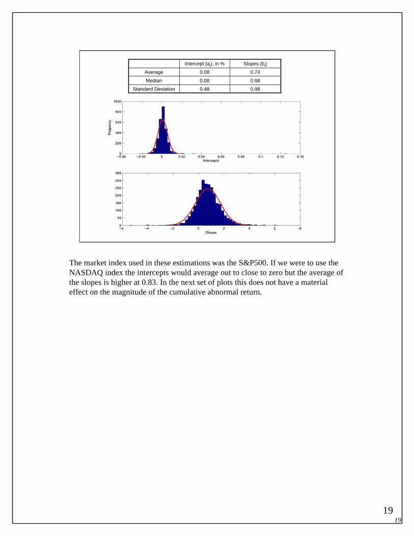
© Alon Brav 2004 Finance 352, Market Efficiency 19
Standard Deviation
Median
Average
0.980.48
0.680.08
0.740.08
Slopes (bt)Intercept (at), in %
The market index used in these estimations was the S&P500. If we were to use the NASDAQ index the intercepts would average out to close to zero but the average of the slopes is higher at 0.83. In the next set of plots this does not have a material effect on the magnitude of the cumulative abnormal return.
2020
© Alon Brav 2004 Finance 352, Market Efficiency 20
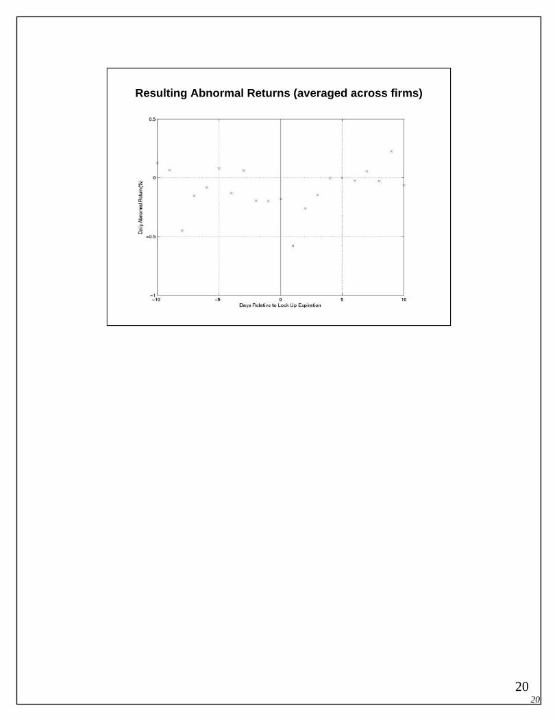
Resulting Abnormal Returns (averaged across firms)
2121
© Alon Brav 2004 Finance 352, Market Efficiency 21
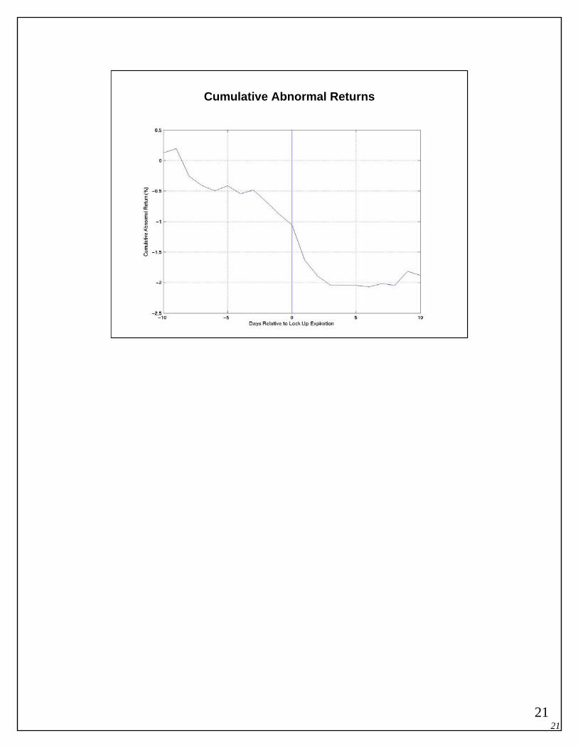
Cumulative Abnormal Returns
2222
© Alon Brav 2004 Finance 352, Market Efficiency 22
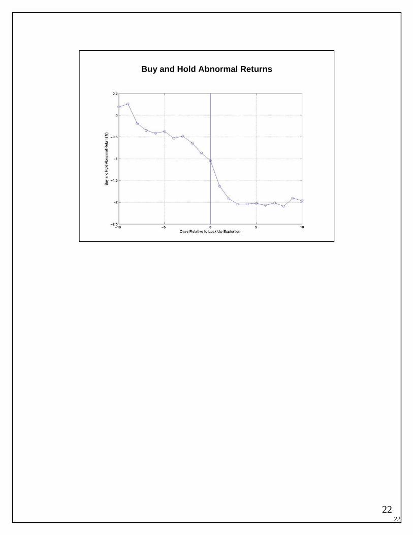
Buy and Hold Abnormal Returns

2323
© Alon Brav 2004 Finance 352, Market Efficiency 23
Event Studies (Continued)
We know from our lecture on asset pricing models that the mannerwith which abnormal returns are calculated can make a big difference. For example, the choice of the CAPM or the Fama French 3 factor model. It has been argued that in practice for short-run event studies, how you control for risk does not matter. Why?
Because for a short run event study, the amount of systematic risk on a day or two is tiny relative to the size of the event. For example, if the market risk premium is 8% per year and there are 250 trading days then the daily premium is .00032, or a little more than 3/100 of a percent a day (3 basis points)
Hence, the joint hypothesis problem is really not an issue and the favorable evidence form short-run event studies has been hailed as supportive of market efficiencyFor long-run event studies, however, the choice of the asset pricing model is crucial.
2424
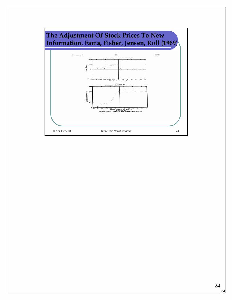
© Alon Brav 2004 Finance 352, Market Efficiency 24
The Adjustment Of Stock Prices To New Information, Fama, Fisher, Jensen, Roll (1969)

2525
© Alon Brav 2004 Finance 352, Market Efficiency 25
Tests of Strong Form Efficiency
Strong form strategies assume you have information that the market does not have.Existence of Insider trading tell us that private information is valuable.In general when an insider buy’s her own stock this is a signal of good future performance.

2626
© Alon Brav 2004 Finance 352, Market Efficiency 26
Caveats
Tests of market efficiency has to consider:The Magnitude Issue: Statistical power. It is simply hard to detect small and economically important deviations from market efficiencyThe Selection Bias Issue: If someone discovered a great money making scheme, they would not publicize it. We are not likely tofind out about schemes that workThe Lucky Find Issue: If you flip a fair coin 50 times, you expect to see 50% heads. If 10,000 people each flip a fair coin 50 times we expect to get at least two of them getting 75% heads. Now, suppose any bet can beat the market 50% of the time. Similarly, suppose 10,000 traders each make 50 bets. We expect to get at least two traders beat the market in 75% of their bets!

2727
© Alon Brav 2004 Finance 352, Market Efficiency 27
The impossibility of informationally efficient markets: Grossman and Stiglitz (1980)
Go through the following logical steps:If markets are perfectly informationally efficient,Then, informed investors cannot profit by analyzing securities’fundamentalsIf it is costly to analyze then informed investors will stop analyzing because they lose money on averageBut, if they stop analyzing information there will be no guarantee that publicly available information is incorporated into prices. Thus, the market won’t be informationally efficientHence, need some expected profit to attract informed investors. These are normal returns to their investments. An efficient amount of inefficiency in the market!

2828
© Alon Brav 2004 Finance 352, Market Efficiency 28
The impossibility of informationally efficient markets (continued)
Is the GS argument consistent with passive investment strategies such as indexing?Should we all buy and hold the S&P500?
An article comparing active versus passive investments see http://www.bernstein.com/Public/story.aspx?cid=1222&nid=185

2929
© Alon Brav 2004 Finance 352, Market Efficiency 29
Market Anomalies (Selected…)
1. The January effect and the Small Firm Effect.2. Predictability in Asset Returns.3. Predictability in Asset Volatility.4. Very short horizon (1 month) Price Reversal.5. Post earnings announcement drift (PEAD).6. Value Line timeliness rank changes.7. Brokerage Analysts' Recommendations. 8. Short horizon (3 to 12 month) price momentum. 9. Long horizon (3-5 year) price reversal and B/M effect.10. Long term performance subsequent to a variety of corporate events
(e.g., IPO, SEOs, Repurchases, dividend initiations and omissions).

3030
© Alon Brav 2004 Finance 352, Market Efficiency 30
The Small Firm Effect
Banz (1981) found that small firms tend to outperform large firms in total and risk-adjusted basis
Divide all NYSE stocks into 5 quintiles according to firm sizeThe average annual return of the firms in the smallest-size quintile was 4.3% higher than the average return of the firms in the largest-size quintile
This is called the Small Firm Effect.

3131
© Alon Brav 2004 Finance 352, Market Efficiency 31
Average Annual Returns By Period
-15%
-10%
-5%
0%
5%
10%
15%
20%
25%
30%
1926
-30
1931
-40
1941
-50
1951
-60
1961
-70
1971
-80
1981
-90
1991
-98
Large Cap Small Cap
3232
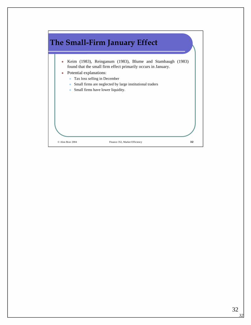
© Alon Brav 2004 Finance 352, Market Efficiency 32
The Small-Firm January Effect
Keim (1983), Reinganum (1983), Blume and Stambaugh (1983) found that the small firm effect primarily occurs in January.Potential explanations:
Tax loss selling in DecemberSmall firms are neglected by large institutional tradersSmall firms have lower liquidity.
3333
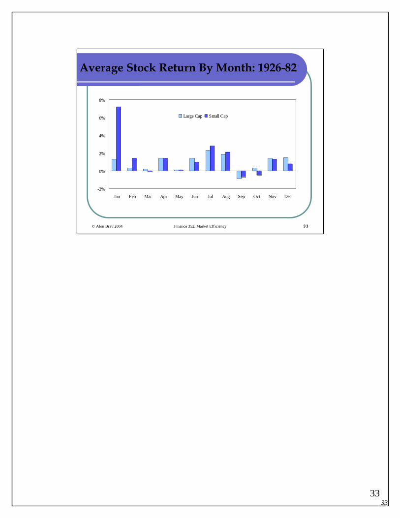
© Alon Brav 2004 Finance 352, Market Efficiency 33
Average Stock Return By Month: 1926-82
-2%
0%
2%
4%
6%
8%
Jan Feb Mar Apr May Jun Jul Aug Sep Oct Nov Dec
Large Cap Small Cap
3434
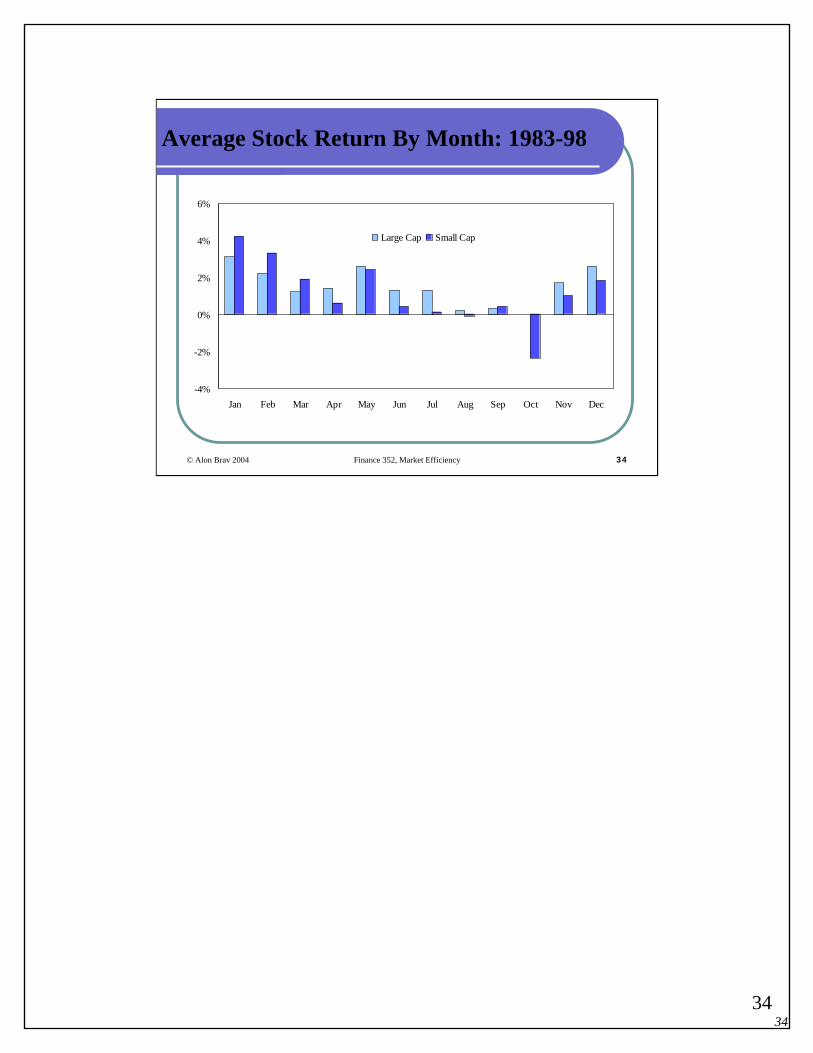
© Alon Brav 2004 Finance 352, Market Efficiency 34
Average Stock Return By Month: 1983-98
-4%
-2%
0%
2%
4%
6%
Jan Feb Mar Apr May Jun Jul Aug Sep Oct Nov Dec
Large Cap Small Cap
3535
© Alon Brav 2004 Finance 352, Market Efficiency 35
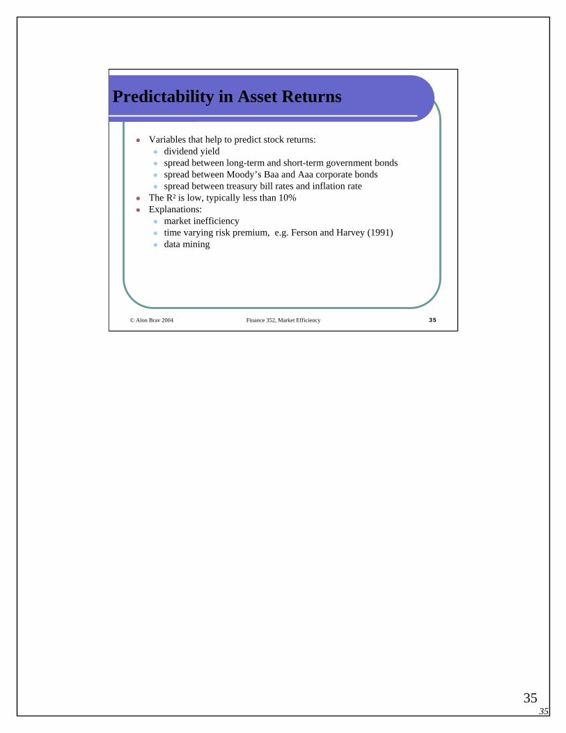
Predictability in Asset Returns
Variables that help to predict stock returns:dividend yieldspread between long-term and short-term government bondsspread between Moody’s Baa and Aaa corporate bondsspread between treasury bill rates and inflation rate
The R² is low, typically less than 10%Explanations:
market inefficiencytime varying risk premium, e.g. Ferson and Harvey (1991)data mining
3636
© Alon Brav 2004 Finance 352, Market Efficiency 36
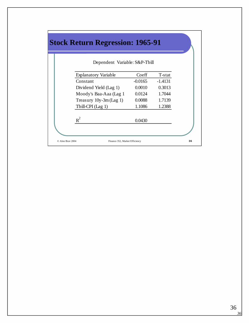
Stock Return Regression: 1965-91
Explanatory Variable Coeff T-statConstant -0.0165 -1.4131Dividend Yield (Lag 1) 0.0010 0.3013Moody's Baa-Aaa (Lag 1 0.0124 1.7044Treasury 10y-3m (Lag 1) 0.0088 1.7139Tbill-CPI (Lag 1) 1.1086 1.2388
R2 0.0430
Dependent Variable: S&P-Tbill
3737
© Alon Brav 2004 Finance 352, Market Efficiency 37
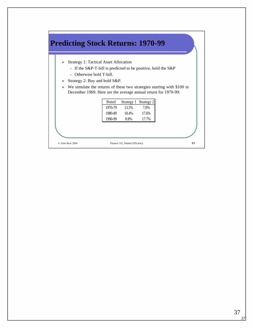
Predicting Stock Returns: 1970-99
Strategy 1: Tactical Asset AllocationIf the S&P-T-bill is predicted to be positive, hold the S&POtherwise hold T-bill.
Strategy 2: Buy and hold S&P.We simulate the returns of these two strategies starting with $100 in December 1969. Here are the average annual return for 1970-99:
Period Strategy 1 Strategy 21970-79 13.5% 7.0%1980-89 18.4% 17.6%1990-99 8.8% 17.7%
3838
© Alon Brav 2004 Finance 352, Market Efficiency 38
Predictability in Asset Volatility
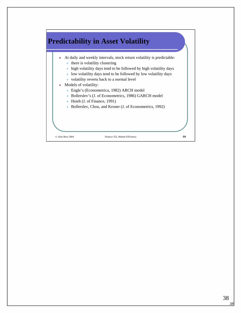
At daily and weekly intervals, stock return volatility is predictable:there is volatility clusteringhigh volatility days tend to be followed by high volatility dayslow volatility days tend to be followed by low volatility daysvolatility reverts back to a normal level
Models of volatility:Engle’s (Econometrica, 1982) ARCH modelBollerslev’s (J. of Econometrics, 1986) GARCH modelHsieh (J. of Finance, 1991)Bollerslev, Chou, and Kroner (J. of Econometrics, 1992)
3939
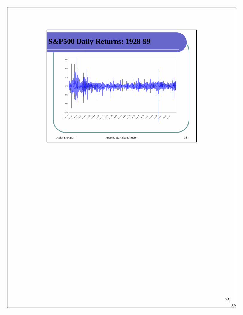
© Alon Brav 2004 Finance 352, Market Efficiency 39
S&P500 Daily Returns: 1928-99
-15%
-10%
-5%
0%
5%
10%
15%
Jan-28
Jan-31
Jan-34
Jan-37
Jan-40
Jan-43
Jan-46
Jan-49
Jan-52
Jan-55
Jan-58
Jan-61
Jan-64
Jan-67
Jan-70
Jan-73
Jan-76
Jan-79
Jan-82
Jan-85
Jan-88
Jan-91
Jan-94
Jan-97
4040
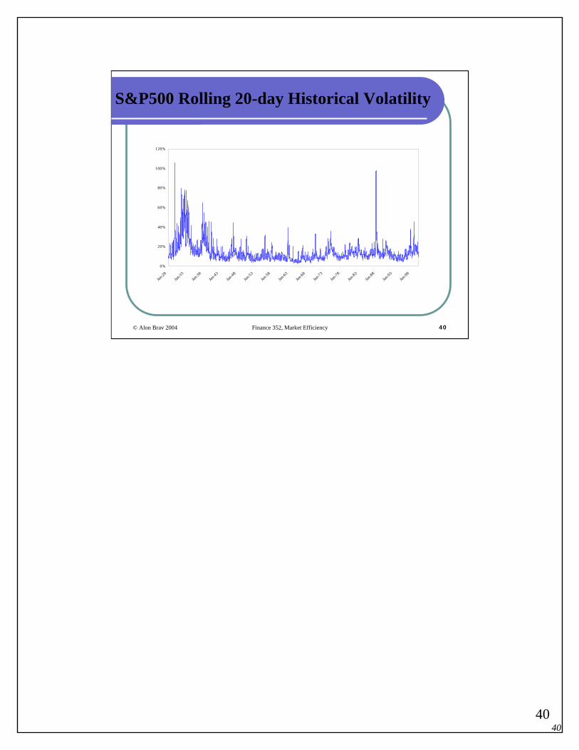
© Alon Brav 2004 Finance 352, Market Efficiency 40
S&P500 Rolling 20-day Historical Volatility
0%
20%
40%
60%
80%
100%
120%
Jan-28
Jan-33
Jan-38
Jan-43
Jan-48
Jan-53
Jan-58
Jan-63
Jan-68
Jan-73
Jan-78
Jan-83
Jan-88
Jan-93
Jan-98
4141
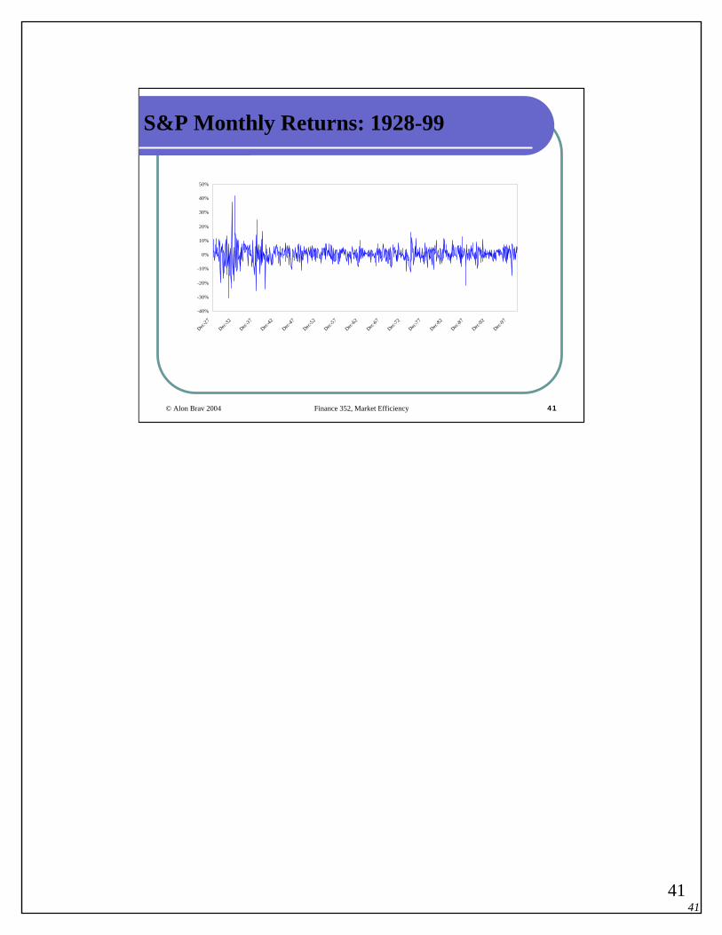
© Alon Brav 2004 Finance 352, Market Efficiency 41
S&P Monthly Returns: 1928-99
-40%
-30%
-20%
-10%
0%
10%
20%
30%
40%
50%
Dec-27
Dec-32
Dec-37
Dec-42
Dec-47
Dec-52
Dec-57
Dec-62
Dec-67
Dec-72
Dec-77
Dec-82
Dec-87
Dec-92
Dec-97
4242
© Alon Brav 2004 Finance 352, Market Efficiency 42
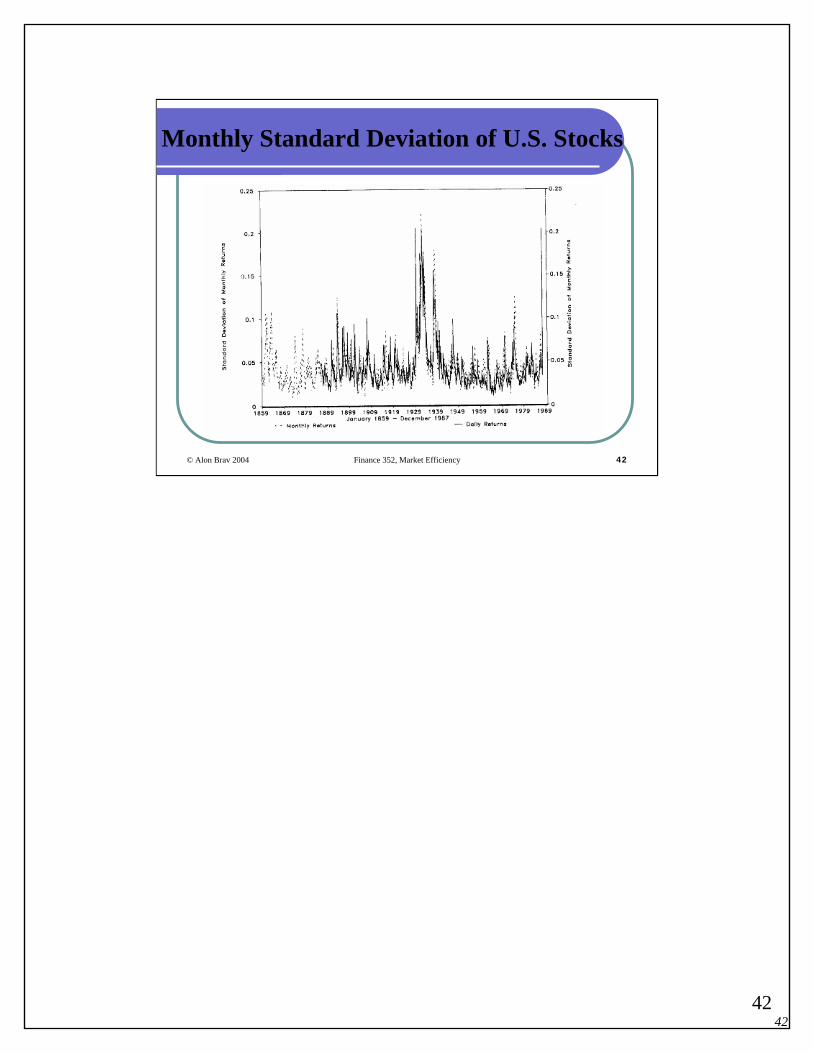
Monthly Standard Deviation of U.S. Stocks

4343
© Alon Brav 2004 Finance 352, Market Efficiency 43
Predicting Asset Volatility
Very strong evidence of volatility clustering in daily returnsMuch weaker evidence of volatility clustering in monthly returnsExchange rates, commodity prices, and bond prices also exhibit this type of behavior
Uses:Short term risk management (Value-at-risk)

4444
© Alon Brav 2004 Finance 352, Market Efficiency 44
Very Short Horizon Reversals
Jegadeesh (J. of Finance, 1990) has found that:At the beginning of each month from 1934 to 1987, divide all stocks into 10 deciles based on their previous month’s return
Decile 1 has the worst performing stocksDecile 10 has the highest performing stocks.
Now look at the return for the current monthDecile 1 has the best performance!Decile 10 has the worst performance!
Likely due to microstructure effects (bid-ask bounce) and probably hard to trade on.

4545
© Alon Brav 2004 Finance 352, Market Efficiency 45
Monthly Return of Decile Portfolios Ranked On Previous Month’s Performance: 1934-87
-1.50%
-1.00%
-0.50%
0.00%
0.50%
1.00%
1.50%
1 2 3 4 5 6 7 8 9 10Deciles
Mon
thly
Ret
urns

4646
© Alon Brav 2004 Finance 352, Market Efficiency 46
Post-Earnings-Announcement Drift (PEAD)
Ball and Brown (1968), Foster, Olsen, Shevlin (1984), Bernard and Thomas (1990)
stocks with large positive (negative) earnings surprises have a positive (negative) price jump on the announcement day and continue to increase (decrease) in price for 13 weeks.

4747
© Alon Brav 2004 Finance 352, Market Efficiency 47
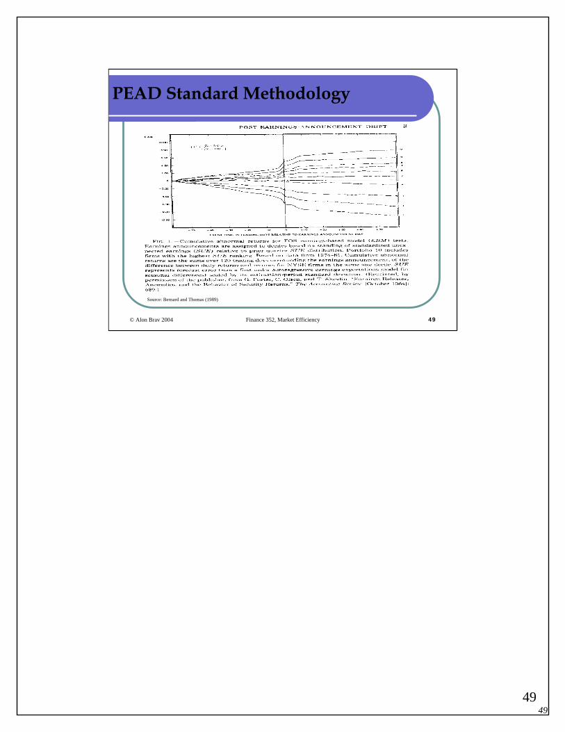
PEAD Standard Methodology
Bernard and Thomas (1990)1974-1986 periodFirms are assigned to one of 10 portfolios based on standardizedunexpected earnings (SUE)
SUE CalculationWe need a proxy for expected earningsRegress current earnings on earnings four quarters ago with a drift term. A seasonal random walk model
EPSt = a + b EPSt-1 + et
We can write down more elaborate time-series modelsConduct the regression firm by firm.

4848
© Alon Brav 2004 Finance 352, Market Efficiency 48
PEAD Standard Methodology
SUE CalculationExpected earnings are therefore:
E(EPSt) = a + b EPSt-1Then, the surprise is the realized EPS (before extraordinary items and discontinued operations) less E(EPSt).The last step is to scale by the estimation standard deviation of the forecast errors to get SUE:SUE = (EPS-EEPS)/(s.d.(error))Why is it necessary to scale by s.d.(error)?
SUE GroupingTake SUE for each firm and group into deciles.Abnormal returns are cumulated beginning the day after the earnings announcement to get the post-earnings announcement drift.
4949
© Alon Brav 2004 Finance 352, Market Efficiency 49
Source: Bernard and Thomas (1989)
PEAD Standard Methodology
5050
© Alon Brav 2004 Finance 352, Market Efficiency 50
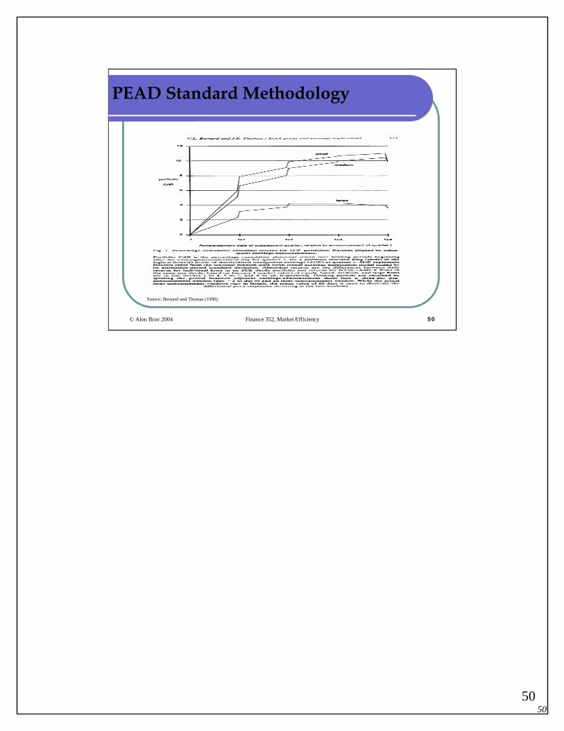
Source: Bernard and Thomas (1990)
PEAD Standard Methodology

5151
© Alon Brav 2004 Finance 352, Market Efficiency 51
PEAD: Results
SUE(10) – SUE(1) earns an abnormal return of 8.6 percent.About a half of average abnormal return is concentrated in the first 60 days following the announcement.In the previous graph Bernard and Thomas sort firms by size intolarge (top 30% NYSE/AMEX), medium (middle 40%) and small (bottom 30%)
For small and medium-sized firms, the effect is even greater: 10%The cumulative returns are about 2/3 as large as the cumulative returns during the quarter up to and including the earnings announcement.

5252
© Alon Brav 2004 Finance 352, Market Efficiency 52
PEAD: Results
About 25% of the effect is concentrated during the next four earnings announcement periods.Stocks held by institutions tend to have less of a drift (controlling for size).Since earnings surprises tend to include both permanent and temporary components, a portion of the initial earnings surprise (about 40%) persists as earnings surprise a quarter later, with progressively smaller amounts later on.The anomaly has been remarkably stable over time and it is not explained, for example, buy either the size or book/market factors (Fama and French (1993)).It seems that the PEAD has declined in the 1990s.

5353
© Alon Brav 2004 Finance 352, Market Efficiency 53
Value Line Timeliness Rank Changes
Weekly rankings of 1700 stocks into 5 groups (1 with the highest prospects and 5 with lowest).Early evidence shows that group 1 earns higher returns than group 5 (Fischer Black, "Yes, Virginia, There is Hope: Tests of the Value Line Ranking System," (1973)).
"It appears that most investment management organizations would improve their performance if they fired all but one of their security analysts and then provided the remaining analyst with the Value Line service." Fischer Black, Professor of Finance at the University of Chicago Graduate School of Business.
Affleck-Graves and Mendenhall (1990) argue that VL rankings follow a PEAD strategy.Stickel (1985) argues that VL analysts provide private information. Information is also stronger for small stocks consistent with Grossman and Stiglitz-type intuition.More recently (post-83) there seems to be less evidence in favor of out-performance of the stocks in group 1. Value line established a mutual fund, The Centurion fund which did not perform well.

5454
© Alon Brav 2004 Finance 352, Market Efficiency 54
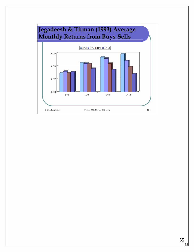
Short Horizon Price Momentum
Jegadeesh and Titman (J. of Finance, 1993) have found that:Over a 3- to 12-month horizon, stock returns have “momentum”:
Good recent performance tends to persistBad recent performance tends to persist
Each quarter from 1965 to 1989, rank stocks in deciles based on the previous L (=3,6,9,12) months’ performance
Go long the highest decile and hold for H (=3,6,9,12) monthsGo short the lowest decile and hold for H months
These long/short portfolios generate abnormal returns! (mainly on the short (losers) portfolio).
5555
© Alon Brav 2004 Finance 352, Market Efficiency 55
Jegadeesh & Titman (1993) Average Monthly Returns from Buys-Sells
0.000
0.005
0.010
0.015
L=3 L=6 L=9 L=12
H=3 H=6 H=9 H=12
5656
© Alon Brav 2004 Finance 352, Market Efficiency 56
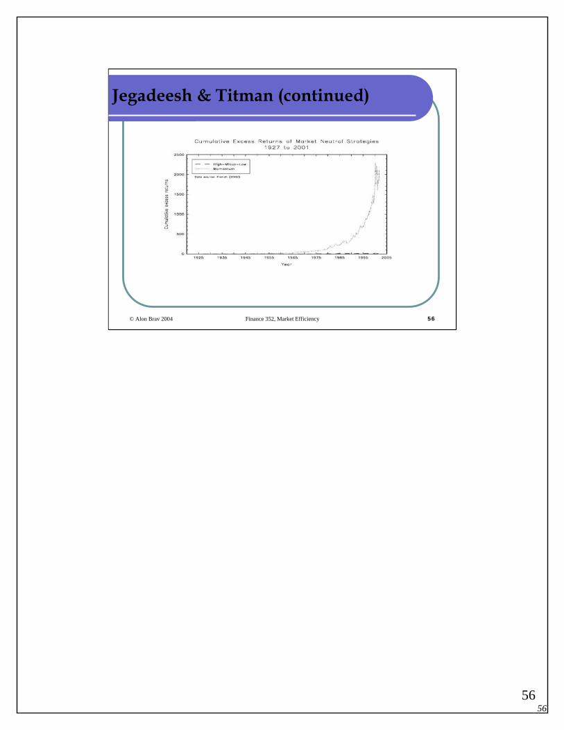
Jegadeesh & Titman (continued)
5757
© Alon Brav 2004 Finance 352, Market Efficiency 57
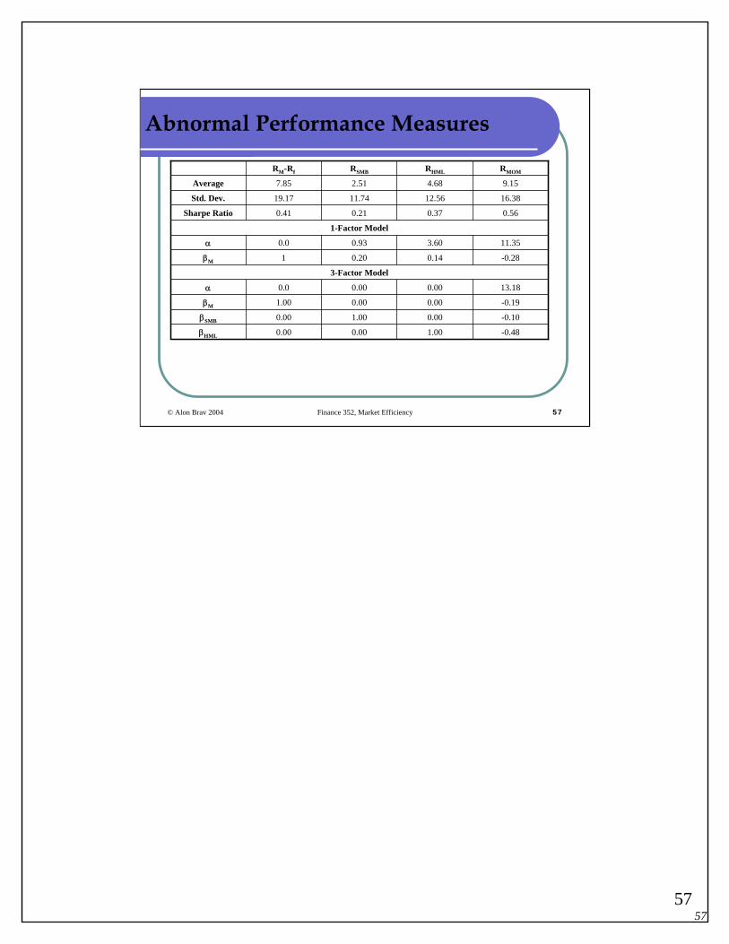
Abnormal Performance Measures
-0.481.000.000.00βHML
-0.100.001.000.00βSMB
-0.190.000.001.00βM
13.180.000.000.0α
3-Factor Model
-0.280.140.201βM
11.353.600.930.0α
1-Factor Model
0.560.370.210.41Sharpe Ratio
16.3812.5611.7419.17Std. Dev.
9.154.682.517.85Average
RMOMRHMLRSMBRM-Rf

5858
© Alon Brav 2004 Finance 352, Market Efficiency 58
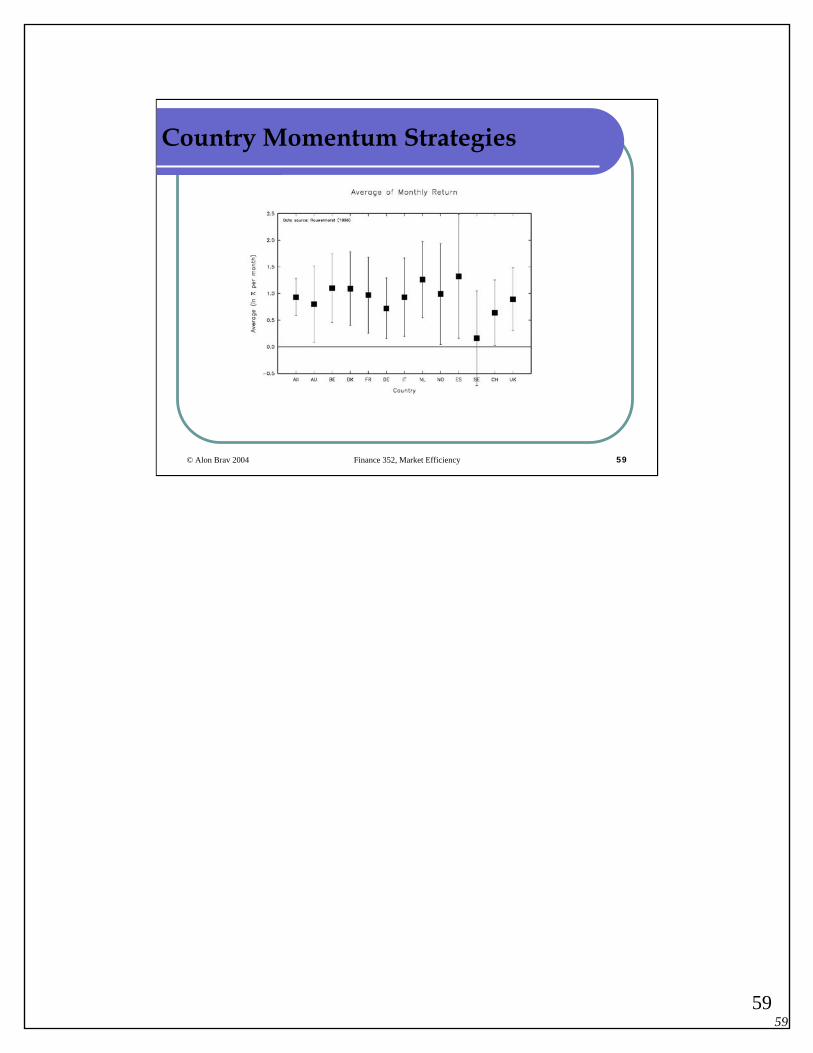
Global Momentum Strategies
5959
© Alon Brav 2004 Finance 352, Market Efficiency 59
Country Momentum Strategies

6060
© Alon Brav 2004 Finance 352, Market Efficiency 60
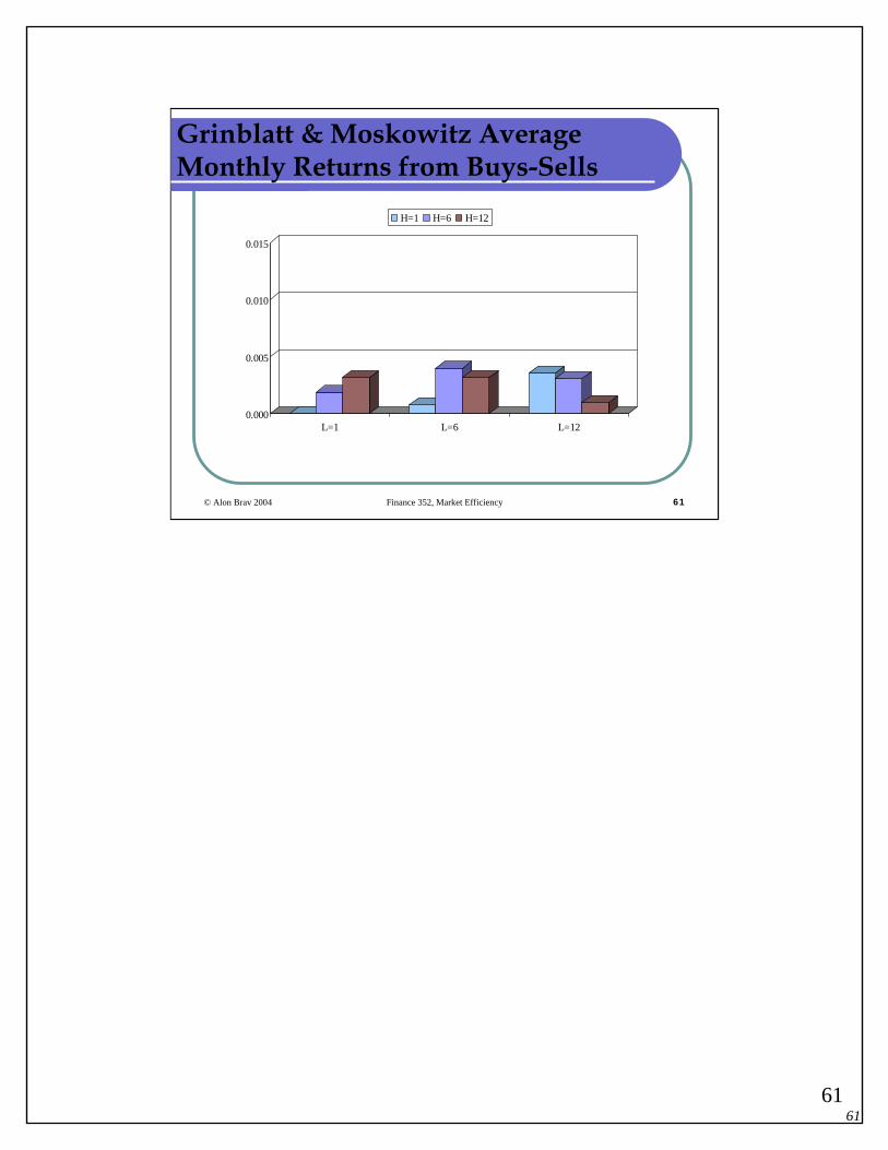
Short Horizon Industry Momentum
Grinblatt and Moskowitz (J. of Finance, 1999) found:There is short horizon momentum in industry portfolios.Each month from July 1963 to July 1995, rank 20 industries based on the previous L months of performance
Go long the top 3 industries and hold for H monthsGo short the bottom 3 industries and hold for H months
These long/short portfolios generate abnormal returns! (mainly on the short (losers) portfolio)
6161
© Alon Brav 2004 Finance 352, Market Efficiency 61
Grinblatt & Moskowitz Average Monthly Returns from Buys-Sells
0.000
0.005
0.010
0.015
L=1 L=6 L=12
H=1 H=6 H=12

6262
© Alon Brav 2004 Finance 352, Market Efficiency 62
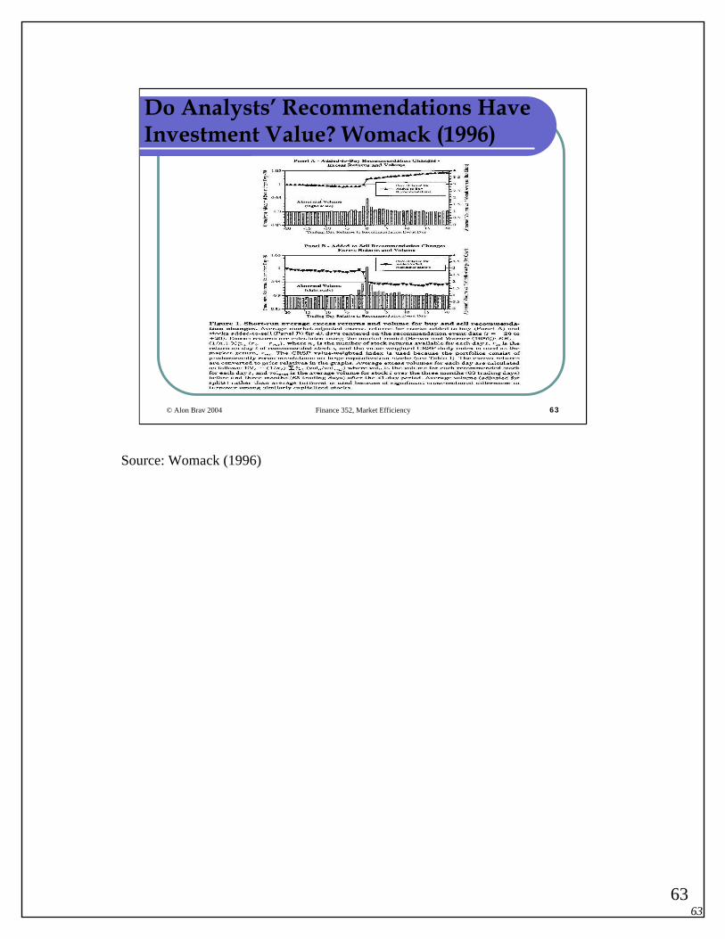
Brokerage Analysts' Recommendations
Does the market incorporate the information in analysts’recommendations?
Womack (1996). Extreme recommendation changesFor Buy (Sell) recommendations event-day abnormal returns are 3% (-4.7%)Post recommendation drift for Buys is significant but short-lived with size-adjusted return of +2.4% over the first post-event month. For Sells, the post-event drift lasts for 6 months and equals -9.1%
Barber, Lehavy, McNichols, and Trueman (1999, 2003). Implement various trading strategies focusing on changes in consensus recommendations.
6363
© Alon Brav 2004 Finance 352, Market Efficiency 63
Do Analysts’ Recommendations Have Investment Value? Womack (1996)
Source: Womack (1996)

6464
© Alon Brav 2004 Finance 352, Market Efficiency 64
Womack (continued)
Source: Womack (1996)
6565
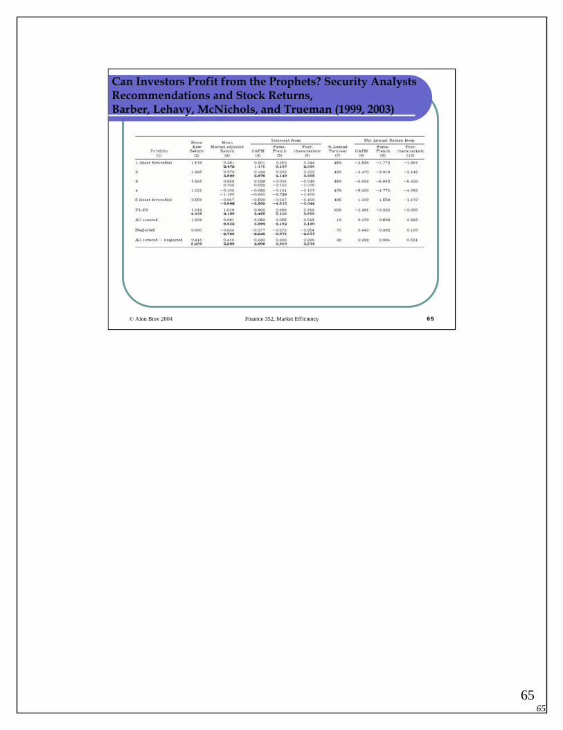
© Alon Brav 2004 Finance 352, Market Efficiency 65
Can Investors Profit from the Prophets? Security Analysts Recommendations and Stock Returns, Barber, Lehavy, McNichols, and Trueman (1999, 2003)
6666
© Alon Brav 2004 Finance 352, Market Efficiency 66
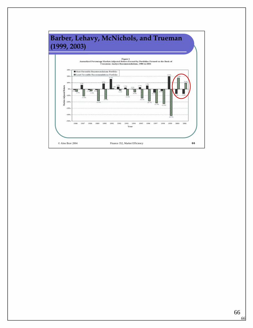
Barber, Lehavy, McNichols, and Trueman (1999, 2003)
6767
© Alon Brav 2004 Finance 352, Market Efficiency 67
Long Horizon Price Reversal
Fama & French (Journal of Political Economy, 1988) found:Over 3- to 5-year horizons, the stock market tends to exhibit negative correlation (reversals)For 17 industries from 1926 to 1985, calculate the autocorrelation coefficients for 1-6, 8, 10 yearsThe autocorrelations for 3,4,5 years are negative and statistically significant!They interpret these findings as evidence in consistent with time-varying expected returns
Cannot rule out Summer’s (1986) view that the mean-reversion is due to irrationality (fads)

6868
© Alon Brav 2004 Finance 352, Market Efficiency 68
Fama & French, Long Horizon Autocorrelations
Portfolio Year 1 Year 2 Year 3 Year 4 Year 5 Year 6 Year 8 Year 10Food -0.01 -0.24 -0.34 -0.36 -0.34 -0.15 0.01 0.08Apparel -0.08 -0.18 -0.20 -0.27 -0.30 -0.21 -0.21 -0.27Drugs -0.02 -0.14 -0.18 -0.12 -0.13 -0.06 -0.09 -0.22Retail -0.01 -0.17 -0.30 -0.32 -0.33 -0.18 -0.10 -0.02Durables 0.02 -0.14 -0.26 -0.33 -0.30 -0.09 0.02 0.13Autos -0.05 -0.22 -0.36 -0.42 -0.35 -0.13 -0.04 -0.02Constructio -0.01 -0.13 -0.27 -0.41 -0.42 -0.21 0.16 0.24Finance -0.01 -0.17 -0.26 -0.25 -0.15 0.07 0.22 0.35Misc -0.02 -0.13 -0.25 -0.35 -0.37 -0.18 0.00 0.12Utilities -0.05 -0.16 -0.27 -0.22 -0.02 0.24 0.14 0.10Transportat -0.10 -0.20 -0.26 -0.33 -0.32 -0.18 -0.09 0.02Bus. Equipm 0.01 -0.22 -0.39 -0.41 -0.36 -0.19 0.05 0.13Chemicals -0.04 -0.33 -0.43 -0.38 -0.37 -0.19 0.01 0.12Metal Prod. 0.01 -0.20 -0.38 -0.49 -0.52 -0.37 -0.16 -0.05Metal Ind. -0.08 -0.27 -0.36 -0.36 -0.35 -0.17 0.18 0.28Mining -0.09 -0.29 -0.37 -0.44 -0.48 -0.28 0.02 0.08Oil -0.02 -0.23 -0.29 -0.42 -0.40 -0.20 0.17 0.27Average -0.03 -0.2 -0.3 -0.34 -0.32 -0.14 0.02 0.08
Table 1. Summary of Multiperiod Autocorrelations (1926-1985): Return Horizons (years 1-6, 8, 10)

6969
© Alon Brav 2004 Finance 352, Market Efficiency 69
A Skeptic’s View of Long Horizon Reversals
However, Richardson (J. of Business & Economic Statistics, 1993)argued that the negative autocorrelations are statistically notimportant. Generate 720 random observations of r(t,t+T).Run the same regression in Fama-French.Look at the largest negative β(T) for T=1,2,3,4,5 years.Repeat this 5,000 times and tabulate the cumulative distributionfunction (CDF).CDF of the Most Negative Autocorrelation:
Mean 0.050 0.250 0.415 0.500 0.585 0.750 0.950-0.022 -0.531 -0.340 -0.234 -0.171 0.170 0.305 0.572
Empirical CDF Values

7070
© Alon Brav 2004 Finance 352, Market Efficiency 70
Long Horizon (3-5 year) Price Reversal and the B/M effect.
DeBondt and Thaler’s (1985) evidence. Past long-term losers earn higher future returns than long-term winners with most of the excess return earned in JanuaryLakonishok, Shleifer and Vishny (1994)
We have already discussed these findings and the possible interpretations
7171
© Alon Brav 2004 Finance 352, Market Efficiency 71
Long-Term Performance of Issuing Firms
Post-issuance, IPOs seem to underperform (Ritter (1991) and Loughran and Ritter (1995)). Here is some empirical evidence based on:
1. IPO information from Professor Jay Ritter at the University of Florida

7272
© Alon Brav 2004 Finance 352, Market Efficiency 72
Time Series of Initial Public Offerings and Underpricing, 1975-2000, (excluding IPOs with an Offer Price less than $5.00)
0100200300400500600700
1975
1977
1979
1981
1983
1985
1987
1989
1991
1993
1995
1997
1999
Time
-20
0
20
40
60
80
100
Underpricing Number of IPOs
Source: Jay Ritter

7373
© Alon Brav 2004 Finance 352, Market Efficiency 73
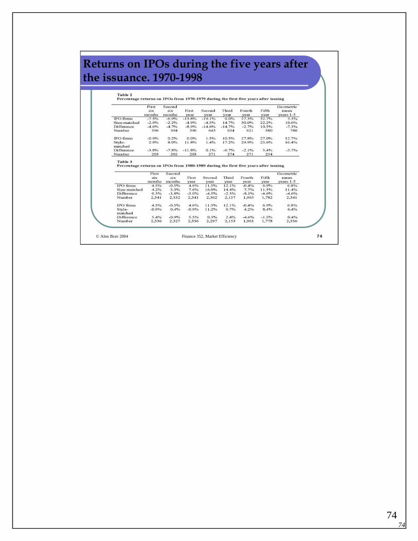
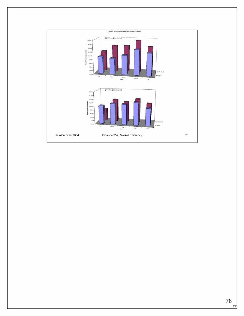
Returns on IPOs during the five years after the issuance. 1970-1998
Source: Jay Ritter
Legend to Table 1:For the first year, the returns are measured from the closing market price on the first day of issue until the sixth month or one-year anniversary. All returns are equally weighted average returns for all IPOs that are still traded on Nasdaq, the Amex, or the NYSE at the start of a period. If an issuing firm is delisted within a year, its return for that year is calculated by compounding the CRSP value-weighted market index for the rest of the year. For the size matched returns, each IPO is matched with a nonissuing firm having the same market capitalization (using the closing market price on the first day of trading for the IPO, and the market capitalization at the end of the previous month for the matching firms). For the size & BM-matched returns, each IPO is matched with a nonissuing firm in the same size decile (using NYSE firms only for determining the decile breakpoints) having the closest book-to market ratio. For the IPOs, book-to-market ratios are calculated using the first recorded post-issue book value and the post-issue market cap calculated using the closing market price on the first CRSP-listed day of trading. For nonissuing firms, the Compustat-listed book value of equity for the most recent fiscal year ending at least four months prior to the IPO date is used, along with the market cap at the close of trading at month-end prior to the month of the IPO with which it is matched. Nonissuing firms are those that have been listed on the Amex-Nasdaq-NYSE for at least five years, without issuing equity for cash during that time. If a nonissuer subsequently issues equity, it is still used as the matching firm. If a nonissuer gets delisted prior to the delisting (or the fifth anniversary, or Dec. 31, 1999), the second-closest matching firm on the original IPO date is substituted, on a point-forward basis. For firms with multiple classes of stock outstanding, market cap is calculated based using only the class in the IPO for the IPO. For nonissuing firms, each class of stock is treated as if it is a separate firm. The sample size is 6,610 IPOs from 1970-1998 when size-matching is used, excluding IPOs with an offer price of less than $5.00, ADRs, REITs, closed-end funds, and unit offers. All IPOs are listed on CRSP for at least 6 months, and after Nasdaq’sinclusion, are listed within six months of going public.
7474
© Alon Brav 2004 Finance 352, Market Efficiency 74
Returns on IPOs during the five years after the issuance. 1970-1998

7575
© Alon Brav 2004 Finance 352, Market Efficiency 75
Returns on IPOs during the five years after the issuance. 1970-1998
7676
© Alon Brav 2004 Finance 352, Market Efficiency 76

7777
© Alon Brav 2004 Finance 352, Market Efficiency 77
Seasoned Equity Offerings, 1975-1992
Equal Weighted Buy-and-Hold Returns (%) Value Weighted Buy-and-Hold Returns (%)
Benchmarks SEO Bench-mark
Abnormal Return
Wealth Relative
SEO Bench-mark
Abnormal Return
Wealth Relative
S&P 500 57.5 87.6 -30.1 0.84 75.3 94.3 -19.0 0.90
Nasdaq Comp. 57.5 76.9 -19.5 0.89 75.3 89.5 -14.2 0.93
CRSP VW 57.5 81.5 -24.0 0.87 75.3 89.5 -14.1 0.93
CRSP EW 57.5 81.6 -24.2 0.87 75.3 102.2 -26.9 0.87
Size and BM (3,775 obs) 57.6 83.9 -26.3 0.86 72.5 97.5 -25.0 0.87
Size, BM, PR12
(3,775 obs) 57.0 84.3 -27.3 0.85 75.7 99.5 -23.8 0.88
What is your prediction regarding the performance subsequent to seasoned equity offerings or “SEOs”? (Loughran and Ritter (1995))
SEO analysis based on 4526 SEOs by 2772 firms over the period 1975-1992
7878
© Alon Brav 2004 Finance 352, Market Efficiency 78
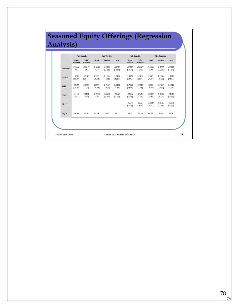
Seasoned Equity Offerings (Regression Analysis)
Full Sample Size Terciles Full Sample Size Terciles
Equal Weighted
Value Weighted
Small Medium Large Equal Weighted
Value Weighted
Small Medium Large
Intercepts -0.0040 [-4.65]
-0.0017 [-1.63]
-0.0069 [-4.17]
-0.0030 [-3.01]
-0.0020 [-2.14] -0.0028
[-3.34] -0.0007 [-0.65]
-0.0050 [-3.04]
-0.0023 [-2.30]
-0.0010 [-1.04]
RMRF 1.0900 [50.39]
0.9345 [36.74]
1.1157 [26.68]
1.1205 [44.61]
1.0336 [42.95] 1.0971
[54.03] 0.9402 [38.01]
1.1269 [28.07]
1.1244 [45.30]
1.0398 [44.83]
SMB 0.7355 [20.42]
0.0514 [1.27]
1.2557 [18.92]
0.7667 [19.23]
0.1848 [4.84] 0.7355
[22.86] 0.0515 [1.31]
1.2558 [19.74]
0.7667 [19.50]
0.1849 [5.03]
HML -0.1183 [-2.83]
0.0171 [0.35]
-0.0064 [-0.08]
-0.2693 [-5.54]
-0.0925 [-1.99] -0.1742
[-4.31] -0.0283 [-0.58]
-0.0820 [-1.03]
-0.3000 [-6.07]
-0.1411 [-3.06]
PR12 -0.2745 [-5.76]
-0.2227 [-3.84]
-0.4339 [-4.61]
-0.1506 [-2.59]
-0.2386 [-4.39]
Adj' R2 94.66 87.68 85.74 93.66 91.35 95.29 88.35 86.85 93.81 91.96

7979
© Alon Brav 2004 Finance 352, Market Efficiency 79
Long-Term Performance of Repurchasing Firms
Ikenberry, Lakonishok, and Vermaelen, 1995, “Market underreaction to open market share Repurchases”, Journal of Financial Economics.
Why would firms repurchase their stock?Signaling Hypothesis: Asymmetric information firm’s insiders and investors. Repurchase announcement is a credible signal. With rational expectations investors should respond immediately in an unbiasedmanner.Underreaction Hypothesis: Less than fully rational reaction which subsequently leads to positive abnormal returns.Data: All repurchases over the period 1980-1990.The benchmark portfolios are i) equal-weighted index, ii) value weighted index, iii) size-based, and iv) size and book-to-market based benchmark.How should we calculate the test statistics? Cumulative abnormal returns or buy and hold returns?Key long-term results: Unconditionally, investing in repurchasing firms leads to positive abnormal returns. Moreover, abnormal return isincreasing in the firms’ book-to-market ratios.

8080
© Alon Brav 2004 Finance 352, Market Efficiency 80
Ikenberry, Lakonishok, and Vermaelen, 1995
8181
© Alon Brav 2004 Finance 352, Market Efficiency 81
Abnormal Performance Subsequent to Dividend Initiations and Omissions
Price Reactions to Dividend Initiations and Omissions: Overreaction or Drift? By Michaely, Thaler, and Womack (1995)
Consistent with the prior literature find that short run price reactions to omissions are greater than for initiations (-7.0% vs. +3.4% three day return)Controlling for the change in the magnitude of dividend yield (which is larger for omissions), the asymmetry shrinks or disappears, depending on the specificationIn the 12 months after the announcement (excluding the event calendar month), there is:
a significant positive market-adjusted return for firms initiating dividends of +7.5% and a significant negative market-adjusted return for firms omitting dividends of -11.0%However, the post dividend omission drift is distinct from and more pronounced than that following earnings surprisesA trading rule employing both samples (long in initiation stocks and short in omission stocks) earns positive returns in 22 out of 25 years
Do firms that omit (initiate) dividends perform as expected given their characteristics?

8282
© Alon Brav 2004 Finance 352, Market Efficiency 82
Summing up...
Three definitions of market efficiency:Markets incorporate various levels of information into security prices.
Random walks and market efficiency.The impossibility of informationally efficient markets: Grossman and Stiglitz (1980).Anomalies. There are still other anomalies we did not cover…
Turn of the Month Effect: Stocks consistently show higher returns on the last day and first four days of the month.The Monday EffectMonday tends to be the worst day to be invested in stocks.Merger related underperformance: Acquiring firms that complete stock mergers underperform while firms that complete cash tender offers do not. One interpretation is that acquirers who use their stock may use it because they believe it to be overvalued.

8383
© Alon Brav 2004 Finance 352, Market Efficiency 83
Anomalies or Data Mining?
Are these real anomalies?Are these data mining?
Data mining:The same data are massaged over and over again. It is not surprising to find something that will “predict” returns.
Final point: Most money managers do not beat the marketMalkiel article
So, if managers do not beat the market, what does that say about market efficiency?

8484
© Alon Brav 2004 Finance 352, Market Efficiency 84
But why it is hard to settle these issues?1) Statistically: No “power”
• We cannot just compare current prices to a reliable fundamental value model to determine the existence of a financial anomaly.

8585
© Alon Brav 2004 Finance 352, Market Efficiency 85
But why it is hard to settle these issues?2) Research design: Returns-Based approach
The central theme of financial economics has been to assume the existence of capital market equilibrium under some model Then test whether the average returns, covariability, and predictability (or lack of) of returns is consistent with that model.
Don’t actually try to “price” assets.Just look to see if price “changes” are behaving according to posited models.

8686
Financial Economists Reject “Fundamental Value”; Embrace Returns Based Research
“Financial economists … work only with hard data and are concerned with the interrelationships between the prices of different financial assets. They ignore what seems to many to be the more important question of what determines the overall level of asset prices. … [There is] a deep distrust of research purporting to explore fundamental valuations.”

8787
© Alon Brav 2004 Finance 352, Market Efficiency 87
But Such Tests Have Very Low Power
“This paper argues that existing evidence does not establish that financial markets are efficient in the sense of rationally reflecting fundamental values. It demonstrates that the types of statistical tests which have been used to date have essentially no power …”

8888
© Alon Brav 2004 Finance 352, Market Efficiency 88
Lessons From Market Efficiency Tests
Can Time Series/Cross Sectional Tests or Volatility Studies Establish Market Efficiency or Inefficiency?
Can Long Run Event Studies Establish Market Efficiency or Inefficiency?
Can Short Run Event Studies Establish Market Efficiency or Inefficiency?
NO
NO
ONLY SOMETIME

8989
© Alon Brav 2004 Finance 352, Market Efficiency 89
Market Efficiency Tests: Bottom Line
• We cannot rely on returns-based tests to tell us whether prices are efficient or not.
• Such tests may reject market efficiency when prices are efficient because we are using the wrong model of market equilibrium (consider FF three-factor model)
• Such tests may fail to reject market efficiency because they assume a model that attributes returns to rational factors (consider same)

9090
© Alon Brav 2004 Finance 352, Market Efficiency 90
Concluding Comments
BKM, Chapter 12:
“We conclude that markets are very efficient, but that rewards to the especially diligent, intelligent, or creative may in fact be waiting.” (page 405)
Top Related