


Languages
Pages
Legal

Managing Uncertainty in Supply Chain: Safety Inventory
Spring, 2014
Supply Chain Management:Strategy, Planning, and Operation
Chapter 11
Byung-Hyun Ha
2
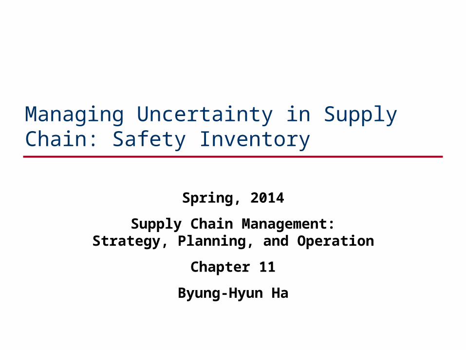
Contents
Introduction
Determining the appropriate level of safety inventory
Impact of supply uncertainty on safety inventory
Impact of aggregation on safety inventory
Impact of replenishment policies on safety inventory
Managing safety inventory in a multi-echelon supply chain
Estimating and managing safety inventory in practice

3
Introduction
Uncertainty in demand Forecasts are rarely completely accurate. If you kept only enough inventory in stock to satisfy average
demand, half the time you would run out.
Safety inventory Inventory carried for the purpose of satisfying demand that
exceeds the amount forecasted in a given period Average inventory = cycle inventory + safety inventory
order arrival
leadtime
order arrival
leadtime
order arrival
leadtime
4
Introduction
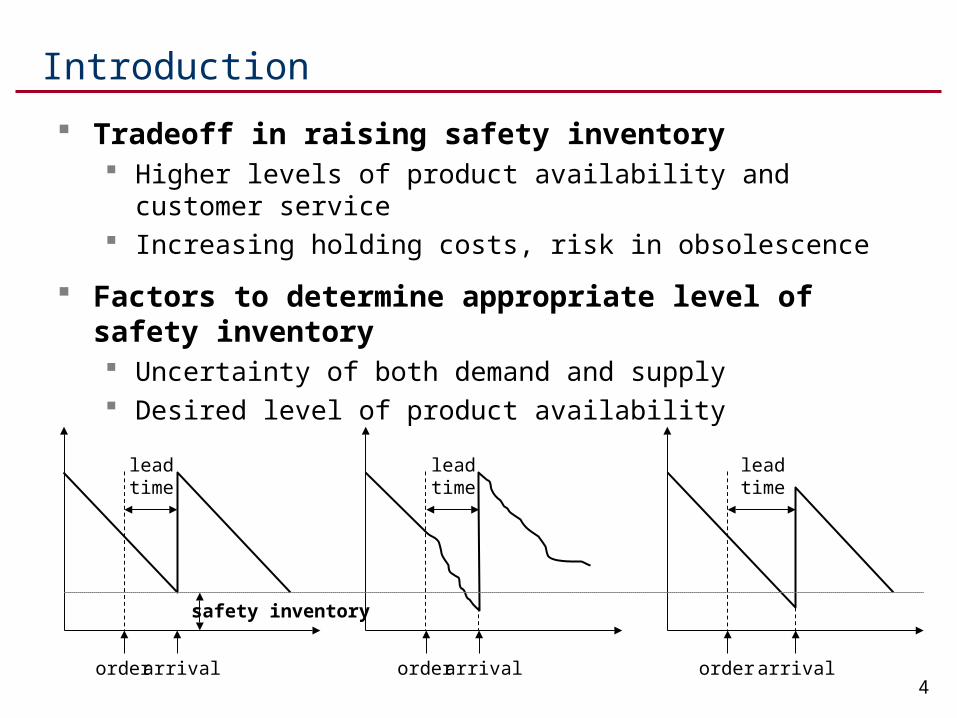
Tradeoff in raising safety inventory Higher levels of product availability and customer service Increasing holding costs, risk in obsolescence
Factors to determine appropriate level of safety inventory Uncertainty of both demand and supply Desired level of product availability
order arrival
leadtime
order arrival
leadtime
order arrival
leadtime
safety inventory
5
Introduction
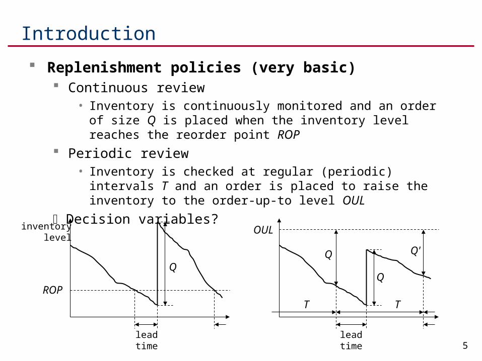
Replenishment policies (very basic) Continuous review
• Inventory is continuously monitored and an order of size Q is placed when the inventory level reaches the reorder point ROP
Periodic review• Inventory is checked at regular (periodic) intervals T and an order is
placed to raise the inventory to the order-up-to level OUL
Decision variables?
leadtime
inventorylevel
Q
ROP
leadtime
Q
OUL
Q
TT
Q'
6
Introduction
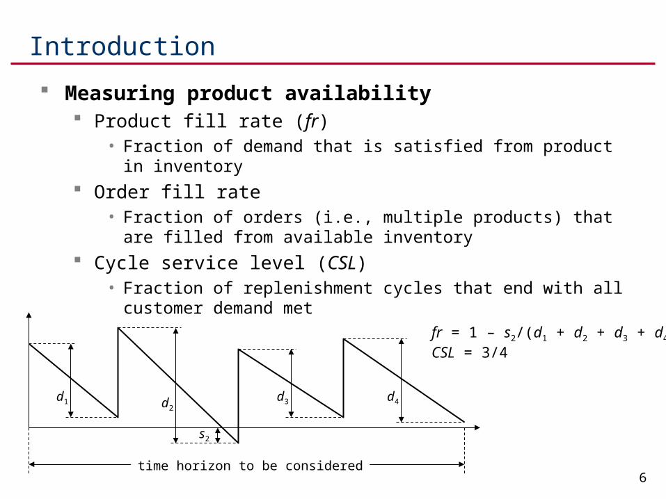
Measuring product availability Product fill rate (fr)
• Fraction of demand that is satisfied from product in inventory
Order fill rate• Fraction of orders (i.e., multiple products) that are filled from availabl
e inventory
Cycle service level (CSL)• Fraction of replenishment cycles that end with all customer demand
met
d1 d2d3 d4
s2
fr = 1 – s2/(d1 + d2 + d3 + d4)CSL = 3/4
time horizon to be considered
7
Determining Level of Safety Inventory
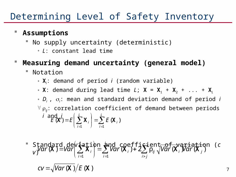
Assumptions No supply uncertainty (deterministic)
• L: constant lead time
Measuring demand uncertainty (general model) Notation
• Xi: demand of period i (random variable)
• X: demand during lead time L; X = X1 + X2 + ... + XL
• Di , i: mean and standard deviation demand of period i
ij: correlation coefficient of demand between periods i and j
Standard deviation and coefficient of variation (cv)
L
ii
L
ii EEE
11
)()( XXX
jijiij
L
ii
L
ii VarVarVarVarVar )()(ρ2)()(
11
XXXXX
)()( XX EVarcv
8
Determining Level of Safety Inventory
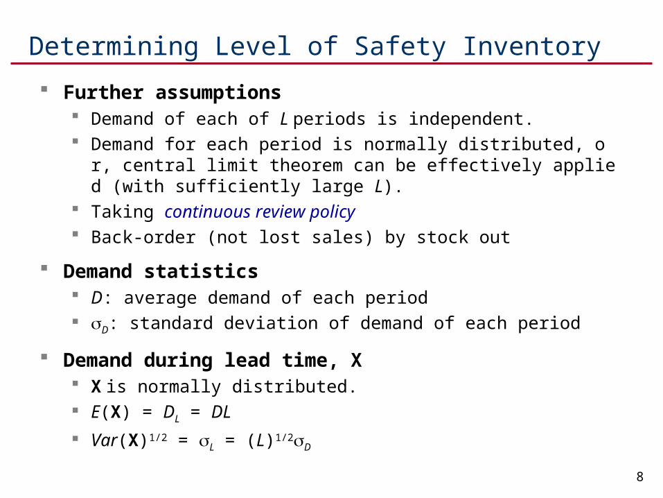
Further assumptions Demand of each of L periods is independent. Demand for each period is normally distributed, or, central limit t
heorem can be effectively applied (with sufficiently large L). Taking continuous review policy Back-order (not lost sales) by stock out
Demand statistics D: average demand of each period D: standard deviation of demand of each period
Demand during lead time, X X is normally distributed. E(X) = DL = DL
Var(X)1/2 = L = (L)1/2D

9
Determining Level of Safety Inventory
Evaluating cycle service level and fill rate Evaluating safety inventory (ss)
• ss = ROP – E(X) = ROP – DL
• Average inventory = Q/2 + ss
order arrival
leadtime
order arrival
leadtime
ROP
ss
E(X) = DL

10
Determining Level of Safety Inventory
Evaluating cycle service level and fill rate Evaluating cycle service level (CSL)
• CSL = Pr(X ROP) = F(ROP) = F(DL + ss)
• where F(x) is the cumulative distribution function of a normally distributed random variable X with mean DL and standard deviation L.
Or• CSL = Pr(X ROP) = Pr((X – DL)/L (ROP – DL)/L)
CSL = Pr(Z ss/L)
CSL = FS(ss/L)
• where Z is a standard normal random variable and FS(z) is the cumulative standard normally distribution function.
11
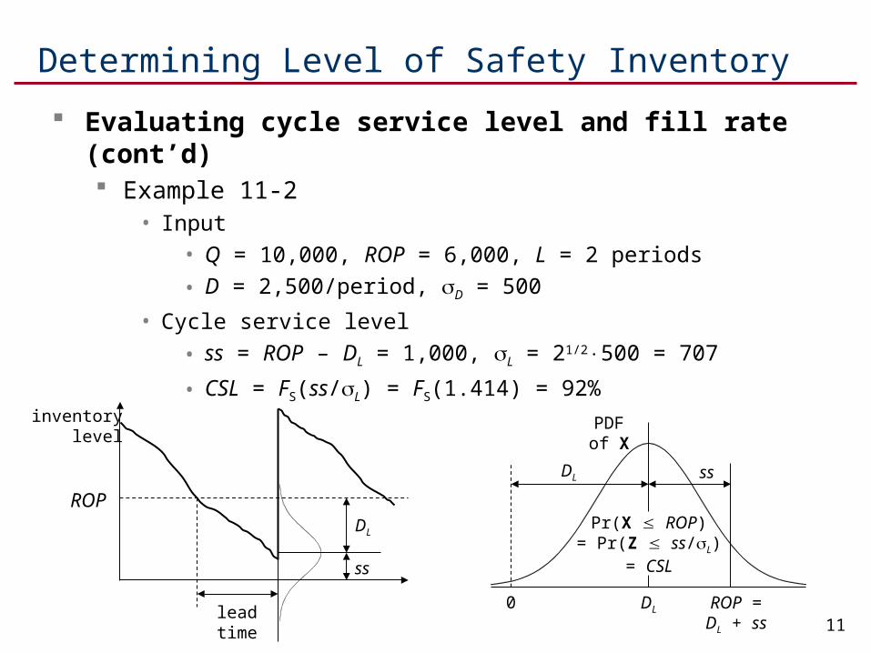
Evaluating cycle service level and fill rate (cont’d) Example 11-2
• Input
• Q = 10,000, ROP = 6,000, L = 2 periods
• D = 2,500/period, D = 500
• Cycle service level
• ss = ROP – DL = 1,000, L = 21/2500 = 707
• CSL = FS(ss/L) = FS(1.414) = 92%
Pr(X ROP)= Pr(Z ss/L)
= CSL
Determining Level of Safety Inventory
leadtime
inventorylevel
ROP
DL
PDFof X
ROP =DL + ss
0
DL
ss
DL ss
12
Determining Level of Safety Inventory
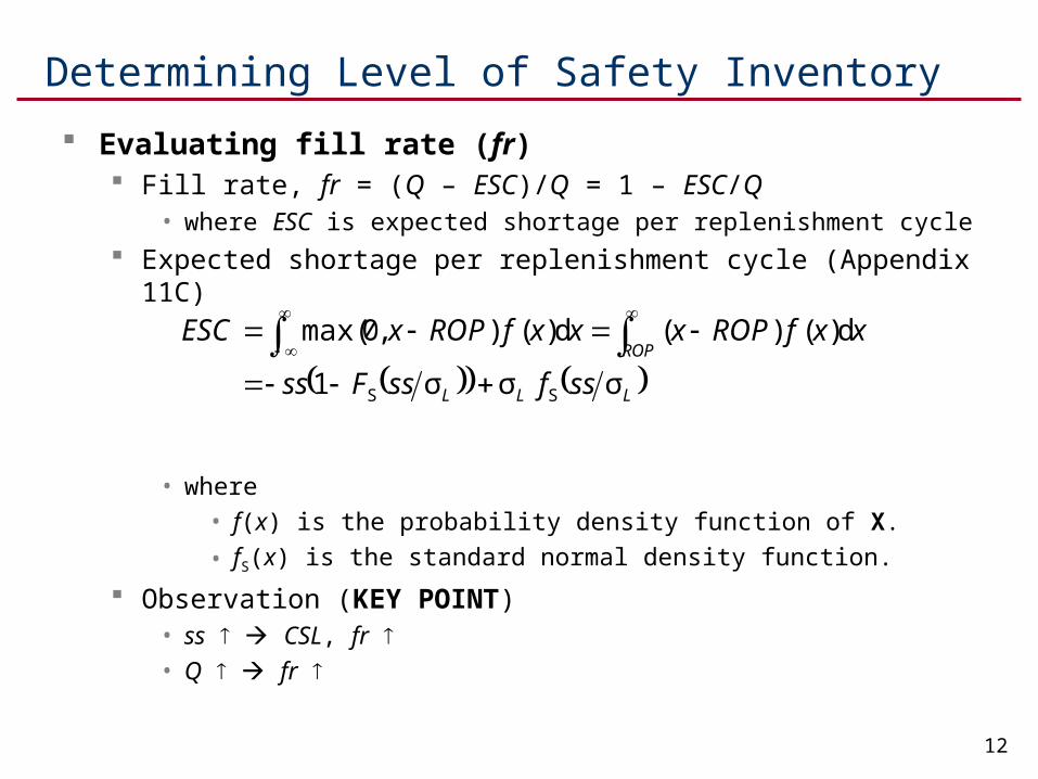
Evaluating fill rate (fr) Fill rate, fr = (Q – ESC)/Q = 1 – ESC/Q
• where ESC is expected shortage per replenishment cycle
Expected shortage per replenishment cycle (Appendix 11C)
• where
• f(x) is the probability density function of X.
• fS(x) is the standard normal density function.
Observation (KEY POINT)• ss CSL, fr • Q fr
LLL
ROP
ssfssFss
xxfROPxxxfROPxESC
σσσ1
d)()(d)(),0max(
SS
13
Determining Level of Safety Inventory
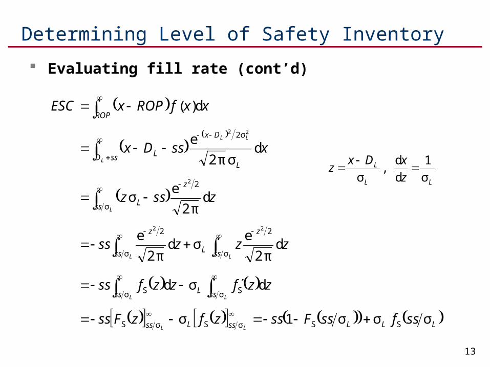
Evaluating fill rate (cont’d)
LLLssLss
ssLss
ss
z
Lss
z
ss
z
L
ssDL
Dx
L
ROP
ssfssFsszfzFss
zzfzzfss
zzzss
zssz
xssDx
xxfROPxESC
LL
LL
LL
L
L
LL
σσσ1σ
dσd
dπ2
eσd
π2
e
dπ2
eσ
dσπ2
e
d)(
SSσSσS
σ Sσ S
σ
2
σ
2
σ
2
σ2
22
2
22
LL
L
z
xDxz
σ
1
d
d,
σ

14
Determining safety inventory given desired CSL Input
• CSL, L
Determining safety inventory, ss• F(ROP) = F(DL + ss) = CSL
ss = F–1(CSL) – DL
Or• FS(ss/L) = CSL
• ss/L = FS–1(CSL)
ss = FS–1(CSL)L
Determining Level of Safety Inventory
f(x)
Pr(X ROP)= Pr(Z ss/L)
= CSL
DL ROP =DL + ss
0
DL ss
15
Determining Level of Safety Inventory
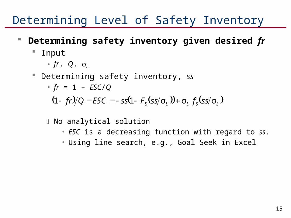
Determining safety inventory given desired fr Input
• fr, Q, L
Determining safety inventory, ss• fr = 1 – ESC/Q
No analytical solution
• ESC is a decreasing function with regard to ss.
• Using line search, e.g., Goal Seek in Excel
LLL ssfssFssESCQfr σσσ11 SS

16
Determining Level of Safety Inventory
Impact of desired product availability on safety inventory
KEY POINT• The required safety inventory grows rapidly with an increase in the d
esired product availability (CSL and fr).
Impact of desired product uncertainty on safety inventory ss = FS
–1(CSL)L = FS–1(CSL)(L)1/2D
KEY POINT• The required safety inventory increases with an increase in the lead
time and the standard deviation of periodic demand.
Reducing safety inventory without decreasing product availability• Reduce supplier lead time, L (e.g., Wal-Mart)
• Reduce uncertainty in demand, L (e.g., Seven-Eleven Japan)
Fill Rate 97.5% 98.0% 98.5% 99.0% 99.5%
Safety Inventory 67 183 321 499 767
17
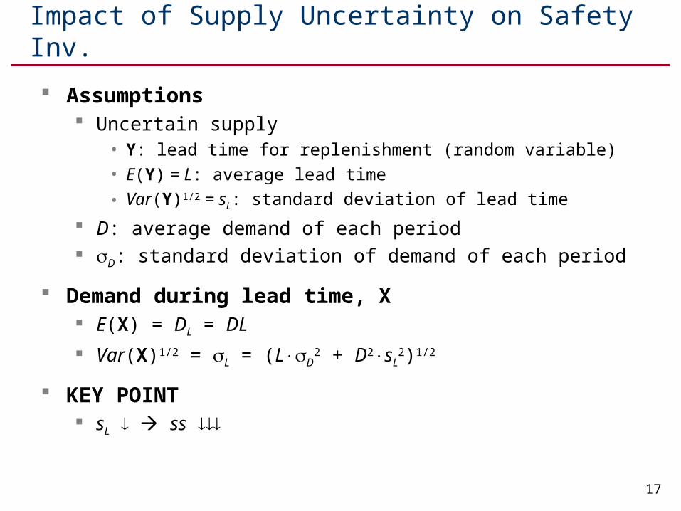
Impact of Supply Uncertainty on Safety Inv.
Assumptions Uncertain supply
• Y: lead time for replenishment (random variable)
• E(Y) = L: average lead time
• Var(Y)1/2 = sL: standard deviation of lead time
D: average demand of each period D: standard deviation of demand of each period
Demand during lead time, X E(X) = DL = DL
Var(X)1/2 = L = (LD2 + D2sL
2)1/2
KEY POINT sL ss

18
Impact of Supply Uncertainty on Safety Inv.
Demand during lead time (cont’d) Let Zl = X1 + X2 + ... + Xl
DLllDllDlEElll
l
111
PrPrPr YYYZX
2222
222222
1
22
1
2
1
222
1
2
1
22
σ
σσ
PrPrσPrσ
PrPr
LsDL
EVarDLEDL
llDlllDll
lEVarlEE
LD
DD
llD
lD
lll
ll
YYY
YYY
YZZYZX
22222 σ LD sDLEEVar XXX

19
Impact of Aggregation on Safety Inventory
Examples HP\Best Buy vs. Dell, Amazon.com vs. Barnes & Noble
Measuring impact Notation
• Di: mean weekly demand in region i, i = 1, ..., k
i: standard deviation of weekly demand in region i, i = 1, ..., k
ij: correlation of weekly demand for regions i and j
• L: lead time in weeks
• CSL: desired cycle service level
Required safety inventory• Decentralized: local inventory in each region
• Centralized: aggregated inventory
k
i iS
k
i iS LCSLFLCSLF1
1
1
1 σσ
jiijjiikiS LCSLF σσρσ
221
1
20
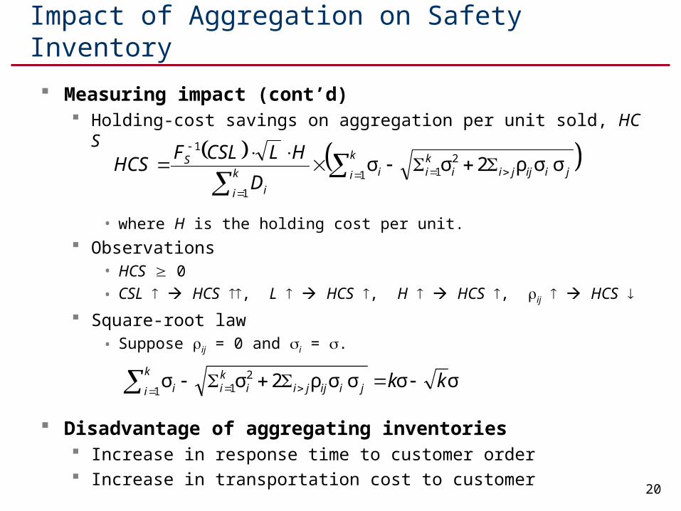
Impact of Aggregation on Safety Inventory
Measuring impact (cont’d) Holding-cost savings on aggregation per unit sold, HCS
• where H is the holding cost per unit.
Observations• HCS 0
• CSL HCS , L HCS , H HCS , ij HCS
Square-root law• Suppose ij = 0 and i = .
Disadvantage of aggregating inventories Increase in response time to customer order Increase in transportation cost to customer
jiijjiiki
k
i ik
i i
S
D
HLCSLFHCS σσρ2σσ 2
11
1
1
σσσσρσσ kkjiijjiiki
k
i i 2211
21
Impact of Aggregation on Safety Inventory
Exploiting benefits from aggregation Information centralization
• Virtual aggregation of inventories
• e.g., McMaster-Carr, Gap, Wal-Mart
Specialization• Items with high cv centralization (usually slow-moving)
• Items with low cv decentralization (usually fast-moving)
• e.g., Barnes & Nobles + barnesandnoble.com
Product substitution• Manufacturer-driven substitution
• Substituting a high-value product for lower-value product that is not in inventory
• No lost sales & savings from aggregation vs. substitution cost
• Customer-driven substitution
• Suggesting a different product instead of out-of-inventory one

22
Impact of Aggregation on Safety Inventory
Exploiting benefits from aggregation (cont’d) Component commonality
• Using common components in a variety of different products
• Safety inventory savings vs. component cost increasing by flexibility
Postponement• Differentiation disaggregated inventories
• Inventory cost savings by delayed differentiation (usually with component commonality)
• Examples
• Dell, Benetton

23
Impact of Replenishment Policy on S. Inv.
Continuous review policy ss = FS
–1(CSL)L
ROP = DL + ss
Q by EOQ formula
Periodic review policy (assuming T is given) ss = FS
–1(CSL)T+L
OUL = DT+L + ss
Optimal T*?
L
Q
OUL
Q
TT
Q'
L
Q'
T

24
Managing Safety Inv. in Multiechelon SC
Two-stage case Inventory relationship
• Supplier’s safety inventory short lead time to retailer retailer’s safety inventory can be reduced
• And vice versa.
Implications• Safety inventories of all stages in multiechelon SC should be related.
Inventory management decision Considering echelon inventory (all inventory between a stage to f
inal customer)• e.g., more retailer safety inventory less required to distributor
Determining stages who carry inventory most• Balancing responsiveness and efficiency!
25
Further Discussion
Role of IT in inventory management Appendix 11D (SKIP)
Estimating and managing safety inventory in practice Account for the fact that supply chain demand is lumpy Adjust inventory policies if demand is seasonal Use simulation to test inventory policies Start with a pilot Monitor service levels Focus on reducing safety inventories
Top Related