


Languages
Pages
Legal

Linking Emergence of the Central Pacific El Niño to the Atlantic Multidecadal Oscillation
JIN-YI YU,* PEI-KEN KAO,1 HOUK PAEK,* HUANG-HSIUNG HSU,# CHIH-WEN HUNG,@ MONG-MING LU,&
AND SOON-IL AN**
* Department of Earth System Science, University of California, Irvine, Irvine, California1Department of Earth System Science, University of California, Irvine, Irvine, California, and Department of Atmospheric Sciences,
National Taiwan University, Taipei, Taiwan#Department of Atmospheric Sciences, National Taiwan University, and Research Center for Environmental Change, Academia Sinica,
Taipei, Taiwan@Department of Geography, National Taiwan Normal University, Taipei, Taiwan&Center for Research and Development, Central Weather Bureau, Taipei, Taiwan
** Department of Atmospheric Sciences, Yonsei University, Seoul, South Korea
(Manuscript received 12 May 2014, in final form 6 October 2014)
ABSTRACT
The ocean–atmosphere coupling in the northeastern subtropical Pacific is dominated by a Pacific meridi-
onal mode (PMM), which spans between the extratropical and tropical Pacific and plays an important role in
connecting extratropical climate variability to the occurrence of El Niño. Analyses of observational data andnumerical model experiments were conducted to demonstrate that the PMM (and the subtropical Pacificcoupling) experienced a rapid strengthening in the early 1990s and that this strengthening is related to anintensification of the subtropical Pacific high caused by a phase change of the Atlantic multidecadal oscillation(AMO). This PMM strengthening favored the development of more central Pacific (CP)-type El Niño events.The recent shift from more conventional eastern Pacific (EP) to more CP-type El Niño events can thus be atleast partly understood as a Pacific Ocean response to a phase change in the AMO.
1. Introduction
The center of warm anomaly associated with El Niñoevents has moved from the eastern Pacific (EP) to cen-tral Pacific (CP) in recent decades (Larkin and Harrison
2005; Yu and Kao 2007; Ashok et al. 2007; Kao and Yu
2009; Kug et al. 2009; Lee and McPhaden 2010; Yu and
Giese 2013; Capotondi et al. 2013). The cause of this
recent emergence of the CPElNiño is not yet known butcould be a consequence of global warming (Yeh et al.
2009) or an expression of natural variability (McPhaden
et al. 2011; Newman et al. 2011). The exact timing of this
location shift has been suggested to be sometime be-
tween the 1980s (Ashok et al. 2007) and the beginning of
the twenty-first century (Lee and McPhaden 2010). Yu
et al. (2012) used three atmospheric and oceanic indices
to argue that the location shift is most obvious around
a period centered on 1993. This early-1990s timeframe is
close to the time when the Atlantic multidecadal oscil-
lation (AMO; Schlesinger and Ramankutty 1994; Kerr
2000) changed its phase. It has been suggested that the
AMO can impact climate not only within the Atlantic
basin but also across the Northern Hemisphere, in-
cluding the Pacific Ocean (e.g., Zhang and Delworth
2007). The possible linkage between the recent emer-
gence of the CP El Niño and the AMO is examined inthis study.We begin describing a possible chain of events
resulting in a shift in the location of El Niño by focusingon variations in the strength of the Pacific meridionalmode (PMM;Chiang andVimont 2004), which is the key
ocean–atmosphere coupling mode of the subtropical
Pacific and plays a crucial role in connecting extra-
tropical climate variability to El Niño generation (e.g.,Anderson 2003; Chiang and Vimont 2004; Alexander
et al. 2006, 2010; Chang et al. 2007). The PMM is char-
acterized by covariability in sea surface temperatures
(SSTs) and surface winds over the northeastern sub-
tropical Pacific. Wind fluctuations associated with
Corresponding author address: Dr. Jin-Yi Yu, Department of
Earth System Science, University of California, Irvine, Irvine, CA
92697-3100.
E-mail: [email protected]
15 JANUARY 2015 YU ET AL . 651
DOI: 10.1175/JCLI-D-14-00347.1
� 2015 American Meteorological Society
extratropical atmospheric variability, in particular the
North Pacific Oscillation (NPO; Walker and Bliss 1932;
Rogers 1981), induce SST anomalies in the subtropical
Pacific via evaporation anomalies. The SST anom-
alies then modify the winds via convection. This wind–
evaporation–SST (WES) feedback mechanism (Xie and
Philander 1994) prolongs and extends the atmosphere-
induced SST anomalies equatorward andwestward from
their generation location in the northeastern subtropical
Pacific toward the tropical central Pacific to form the
spatial pattern of the PMM. The atmosphere–ocean
coupling also sustains the PMM from boreal winter,
when the extratropical atmospheric variability is stron-
gest (e.g., Vimont et al. 2001, 2003), to the following
seasons, which explains how the extratropical variability
in winter can trigger the development of El Niño eventsin the following spring or summer.More recently, the PMM and its associated subtrop-
ical coupling were suggested to play a particularly im-
portant role in exciting the CP El Niño (Yu and Kim
2011; Kim et al. 2012; Lin et al. 2014). In contrast to the
conventional EP type of El Niño that is characterized bySST anomalies extending westward from the SouthAmerican coast with decreasing amplitude, the CP ElNiño has most of its SST anomalies confined around theinternational date line. While the generation of the EPEl Niño involves traditional El Niño dynamics that em-phasize equatorial Pacific thermocline variations (e.g.,Suarez and Schopf 1988; Battisti and Hirst 1989; Jin
1997), the generation of the CP El Niño has been linkedby some to forcing from the extratropical atmosphere(Yu and Kim 2011; Yu et al. 2011, 2012; Kim et al. 2012;
Lin et al. 2014). The extratropical atmospheric forcing is
suggested to penetrate into the tropical central Pacific
through the PMM via the WES feedback mechanism.
Since the CP El Niño has occurred more frequently inrecent decades, it is natural to wonder whether the PMMhas also experienced similar decadal variations and howthese variations, if any, might be related to leadingmodes of decadal variability, including theAMOand thePacific decadal oscillation (PDO; Mantua et al. 1997).
Statistical analyses using observational and reanalysis
data and numerical experiments using an atmospheric
general circulation model (AGCM) coupled with a slab
ocean were performed to answer these questions. It
should be noted that zonal advection in the tropical
Pacific has also been suggested to be important to the
generation of CP El Niño events (e.g., Kug et al. 2009;
Yu et al. 2010) and can extend the PMM-induced
warming in the central Pacific eastward leading to EP
El Niño events (e.g., Alexander et al. 2010). Neverthe-
less, a recent study reported that the PMM and its sub-
tropical coupling seem more linked to the generation of
the CP El Niño than to the EP El Niño in the multiplecoupled GCM simulations (Lin et al. 2014). In this
study, the possible role of zonal ocean advection is not
examined.
2. Datasets
In this study, datasets used for analysis include the
monthly 10-m winds and sea level pressure (SLP) from
the National Centers for Environmental Prediction–
National Center for Atmospheric Research (NCEP–
NCAR) reanalysis dataset (Kalnay et al. 1996) and SSTs
from National Oceanic and Atmospheric Administra-
tion (NOAA) Extended Reconstructed Sea Surface
Temperature dataset (ERSST; Smith et al. 2008). Spe-
cifically, data for the period 1948–2010 were analyzed.
Monthly anomalies were obtained by removing the
seasonal cycles and linear trends. To validate the results
obtained from the NCEP–NCAR reanalysis, we also
used the Twentieth Century Reanalysis (20CR; Compo
et al. 2011) and the Japanese 55-year Reanalysis Project
(JRA-55; Ebita et al. 2011).
Two indices for decadal variability modes were used
in this study: the PDO index and the AMO index. The
PDO index was defined as the leading principal com-
ponent (PC) of an empirical orthogonal function (EOF)
mode of monthly SST anomalies in the North Pacific
(poleward of 208N) after removing the global-mean SST
anomalies (Mantua et al. 1997). The AMO index was
defined as the linearly detrended area-averaged SST
anomalies over the North Atlantic (08–708N) (Enfield
et al. 2001).
A set of the Atmospheric Model Intercomparison
Project (AMIP; Gates et al. 1999) model output in phase
5 of the Coupled Model Intercomparison Project
(CMIP5; Taylor et al. 2012) as summarized inTable 1was
also used to gain insight into the observational findings.
3. Results
To identify the PMM, a singular value decomposition
(SVD; Bretherton et al. 1992) analysis was applied to the
cross-covariance between SST and 10-mwind anomalies
in the northeastern subtropical Pacific (208S–308N,
1758E–958W). We removed the ENSO signals (re-
gressions of SST and 10-m wind anomalies with an index
of ENSO) from the original anomalies before the SVD
analysis. Following Chiang andVimont (2004), we chose
to use the cold tongue index (CTI; SST anomalies av-
eraged over 68S–68N, 1808–908W) to remove the El Niñoinfluence. It should be noted that this is not an op-timal way to remove the ENSO signals. Compo and
Sardeshmukh (2010) and Solomon and Newman (2012)
652 JOURNAL OF CL IMATE VOLUME 28
have developed methods that can better remove the full
spatial structure and evolution of the ENSO signals us-
ing a linear inverse modeling approach. Nevertheless,
the domain of the CTI index covers not only the EP
ENSO region (i.e., Niño-3 region) but also a large part ofthe CP ENSO region (i.e., Niño-4 region) and is suitablefor the purpose of this study.The leading SVD mode shown in Fig. 1a depicts the
PMM’s SST and wind anomaly patterns during the peak
season of the PMM [i.e., March–May (MAM)]. The
pattern is characterized by positive SST anomalies and
southwesterly wind anomalies extending from the Baja
California coast to the tropical central Pacific. The
southwesterly wind anomalies represent a weakening of
the climatological northeasterly trade winds in the
northern subtropics and are collocated with positive SST
anomalies because of the reduced surface evaporation
associated with the weaker trade winds. A pair of PCs
was also produced as part of the SVD analysis. The PCs
represent the temporal variations of the PMM-associated
SST and surface wind anomalies and are referred to, re-
spectively, as the PMM SST and wind indices.
Since the PMM is a mode of coupled atmosphere–
ocean variability, its strength can be represented by the
correlation coefficient between the PMM SST and wind
indices. This correlation during MAM is calculated us-
ing a 10-yr window running from 1948 to 2010. As shown
in Fig. 1b, the correlation (i.e., the PMM strength)
drops briefly around 1960, 1976, and 1993 to divide
1962–2004 into three periods: 1962–72 (period I), 1977–
88 (period II), and 1993–2004 (period III).We only focus
on the period from 1962, as the data prior to period I are
too short. The PMM strength shows a stepwise increase,
starting from a relatively weak state during periods I and
II and then jumping to a strong state during period III.
The mean correlation substantially increases from pe-
riods I and II (0.73 for both periods) to period III (0.86).
With a stringent test, the difference in the mean PMM
strength between period III and the other two periods
passes the 90% confidence level using a one-tailed
Student’s t test. The robustness of this early-1990s
strengthening was validated by repeating the SVD and
correlation analyses with two additional reanalysis
products: the 20CR and JRA-55. A significant and
similar early-1990s jump in the correlation was found in
these two additional datasets (Figs. 1c,d). It is important
to note that this early-1990s strengthening of the PMM
coincides with the time when the El Niño was de-termined to shift from being predominantly of the EPtype to being predominantly of the CP type (Yu et al.
2012). Investigating the cause of this strengthening will
help to understand why the CP El Niño has occurredmore frequently in recent decades.
To understand why the PMM strength has varied, we
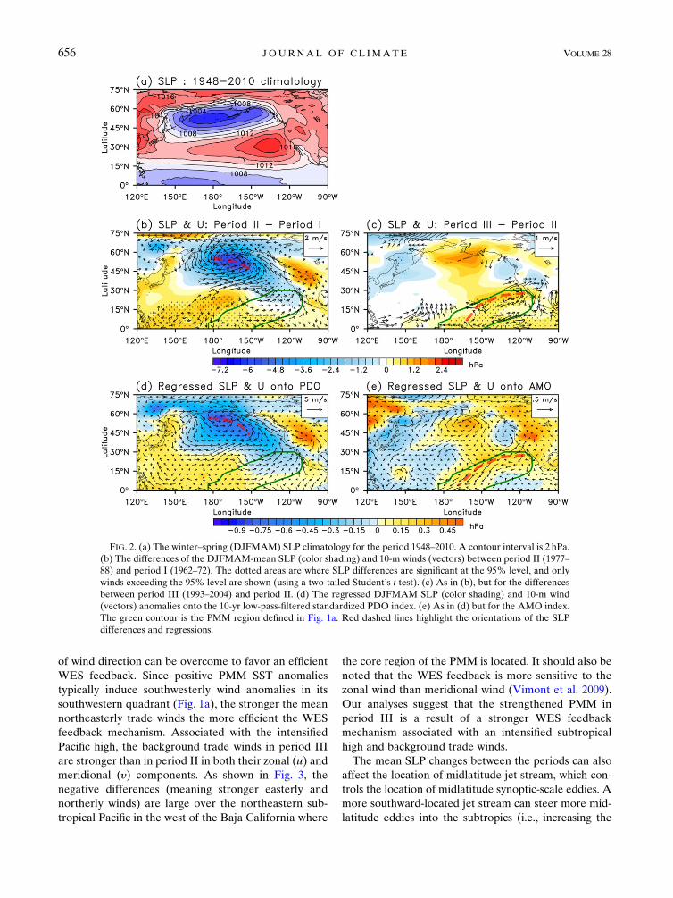
examined in Fig. 2 the mean SLP and 10-m wind states
during each of the three periods during the boreal
winter–spring seasons [December–May (DJFMAM)].
These are the seasons when the PMM typically develops
and peaks (e.g., Chiang and Vimont 2004). The SLP
climatology in these seasons (Fig. 2a) is characterized by
an Aleutian low over the North Pacific and a Pacific
subtropical high over the eastern subtropics. The change
in the mean SLP (color shading) from period I to II
(Fig. 2b) is dominated by an intensification of the
Aleutian low with a particular northwest–southeast
orientation (highlighted by a red dashed line). This SLP
change was accompanied by cyclonic wind anomalies
(vectors). In contrast, the change in the mean SLP from
period II to III (Fig. 2c) is dominated by a weakening of
the Aleutian low and an intensification of the sub-
tropical high. The intensified high is centered in the
eastern Pacific and extends southwestward to the trop-
ical central Pacific. This particular northeast–southwest
orientation is highlighted in Fig. 2c by a red dashed line.
The SLP change was accompanied by anticyclonic wind
anomalies that strengthened the mean northeasterly
trade winds. In the figure, we use a green contour to
highlight the location of the PMM (i.e., Baja California
to the tropical central Pacific) from Fig. 1a; it is clear that
this region overlaps with the region where the most
significant changes occur in the background trade winds
and SLP from period II to III. This overlapping indicates
that the SLP and trade wind changes are likely to affect
the strength of the PMM. Although the mean SLP
changes from period I to II also appear in the subtropical
Pacific region (see Fig. 2b), they overlap only with the
northern portion of the PMM region and are less likely
to affect the strength of the PMM.
The significant changes in the subtropical high and its
associated trade winds have important implications for
the WES feedback mechanism that supports the PMM.
The relationship between latent heat flux anomalies and
surface wind anomalies is an important component of
the WES feedback, which can be expressed by the fol-
lowing relationship according to Czaja et al. (2002) and
Vimont et al. (2009):
dLH
du;
uffiffiffiffiffiffiffiffiffiffiffiffiffiffiffiffiffiu21w2
*
q 51ffiffiffiffiffiffiffiffiffiffiffiffiffiffiffiffiffiffiffiffiffiffi
11�w*u
�2r , (1)
where dLH is the latent heat flux variation caused by the
zonal wind variation (du) for a given mean zonal wind
state (u) and turbulent background wind speed (w*).
Here, for simplicity and explanatory purposes, we ne-
glect the meridional wind in the equation. The efficiency
15 JANUARY 2015 YU ET AL . 653
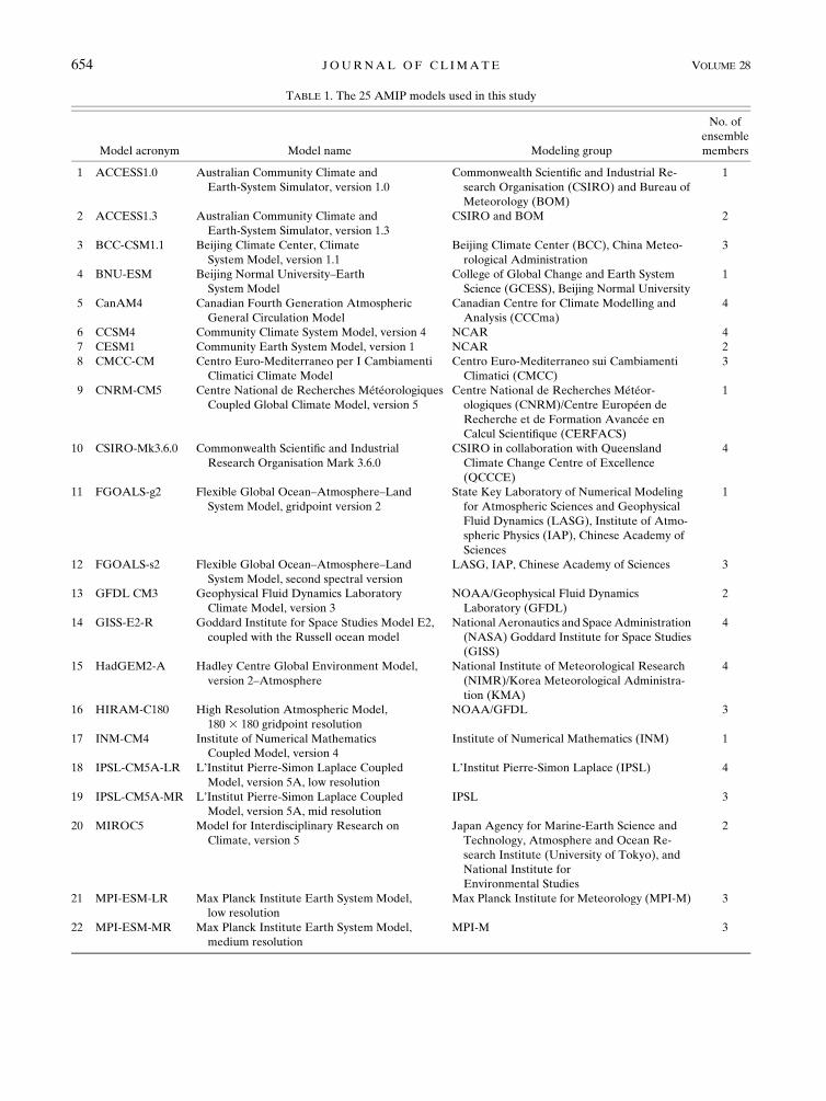
TABLE 1. The 25 AMIP models used in this study
Model acronym Model name Modeling group
No. of
ensemble
members
1 ACCESS1.0 Australian Community Climate and
Earth-System Simulator, version 1.0
Commonwealth Scientific and Industrial Re-
search Organisation (CSIRO) and Bureau of
Meteorology (BOM)
1
2 ACCESS1.3 Australian Community Climate and
Earth-System Simulator, version 1.3
CSIRO and BOM 2
3 BCC-CSM1.1 Beijing Climate Center, Climate
System Model, version 1.1
Beijing Climate Center (BCC), China Meteo-
rological Administration
3
4 BNU-ESM Beijing Normal University–Earth
System Model
College of Global Change and Earth System
Science (GCESS), Beijing Normal University
1
5 CanAM4 Canadian Fourth Generation Atmospheric
General Circulation Model
Canadian Centre for Climate Modelling and
Analysis (CCCma)
4
6 CCSM4 Community Climate System Model, version 4 NCAR 4
7 CESM1 Community Earth System Model, version 1 NCAR 2
8 CMCC-CM Centro Euro-Mediterraneo per I Cambiamenti
Climatici Climate Model
Centro Euro-Mediterraneo sui Cambiamenti
Climatici (CMCC)
3
9 CNRM-CM5 Centre National de Recherches MétéorologiquesCoupled Global Climate Model, version 5
Centre National de Recherches Météor-ologiques (CNRM)/Centre Européen deRecherche et de Formation Avancée enCalcul Scientifique (CERFACS)
1
10 CSIRO-Mk3.6.0 Commonwealth Scientific and Industrial
Research Organisation Mark 3.6.0
CSIRO in collaboration with Queensland
Climate Change Centre of Excellence
(QCCCE)
4
11 FGOALS-g2 Flexible Global Ocean–Atmosphere–Land
System Model, gridpoint version 2
State Key Laboratory of Numerical Modeling
for Atmospheric Sciences and Geophysical
Fluid Dynamics (LASG), Institute of Atmo-
spheric Physics (IAP), Chinese Academy of
Sciences
1
12 FGOALS-s2 Flexible Global Ocean–Atmosphere–Land
System Model, second spectral version
LASG, IAP, Chinese Academy of Sciences 3
13 GFDL CM3 Geophysical Fluid Dynamics Laboratory
Climate Model, version 3
NOAA/Geophysical Fluid Dynamics
Laboratory (GFDL)
2
14 GISS-E2-R Goddard Institute for Space Studies Model E2,
coupled with the Russell ocean model
National Aeronautics and SpaceAdministration
(NASA) Goddard Institute for Space Studies
(GISS)
4
15 HadGEM2-A Hadley Centre Global Environment Model,
version 2–Atmosphere
National Institute of Meteorological Research
(NIMR)/Korea Meteorological Administra-
tion (KMA)
4
16 HIRAM-C180 High Resolution Atmospheric Model,
180 3 180 gridpoint resolution
NOAA/GFDL 3
17 INM-CM4 Institute of Numerical Mathematics
Coupled Model, version 4
Institute of Numerical Mathematics (INM) 1
18 IPSL-CM5A-LR L’Institut Pierre-Simon Laplace Coupled
Model, version 5A, low resolution
L’Institut Pierre-Simon Laplace (IPSL) 4
19 IPSL-CM5A-MR L’Institut Pierre-Simon Laplace Coupled
Model, version 5A, mid resolution
IPSL 3
20 MIROC5 Model for Interdisciplinary Research on
Climate, version 5
Japan Agency for Marine-Earth Science and
Technology, Atmosphere and Ocean Re-
search Institute (University of Tokyo), and
National Institute for
Environmental Studies
2
21 MPI-ESM-LR Max Planck Institute Earth System Model,
low resolution
Max Planck Institute for Meteorology (MPI-M) 3
22 MPI-ESM-MR Max Planck Institute Earth System Model,
medium resolution
MPI-M 3
654 JOURNAL OF CL IMATE VOLUME 28

of the WES feedback (i.e., dLH/du) can be affected by
the ratio of the turbulent background wind to the mean
zonal wind (w* /u) in the denominator on theRHS of the
equation. According to the equation, the stronger the
backgroundwind (u), the smaller the ratio and the larger
the WES feedback efficiency. Physically, the WES
feedback mechanism is known to work when the wind
anomalies induced by convection are in a direction op-
posite to that of the mean winds (Xie 1999). In order for
the WES feedback to work more efficiently, the mean
wind (u) should not change direction. However, the
mean wind direction can be reversed by the background
disturbances (w*). Therefore, the stronger the mean
zonal wind (u), the more easily the disturbance reversal
FIG. 1. (a) The leading SVD mode of SST (color shading) and 10-m wind (vectors) anomalies for the PMM in
boreal spring (MAM). Red (blue) shading indicates positive (negative) values with an interval of 0.18C. The green
contour is the 0.28C isotherm representing the PMM region. (b) 10-yr running correlation coefficients between the
PMMSST andwind indices. The red line indicates amean of the correlation coefficients during each period. The gray
shading is used to emphasize three different periods (1962–72, 1977–88, and 1993–2004). The shadings at the top and
bottom are the positive (red) and negative (blue) phases of the 10-yr low-pass-filtered PDO and AMO, respectively.
(c),(d) As in (b), but for (c) 20CR and (d) JRA-55.
TABLE 1. (Continued)
Model acronym Model name Modeling group
No. of
ensemble
members
23 MRI-AGCM2H Meteorological Research Institute
Atmospheric General Circulation Model,
version 2 (high resolution)
Meteorological Research Institute (MRI) 3
24 MRI-CGCM3 Meteorological Research Institute Coupled
Atmosphere–Ocean General Circulation
Model, version 3
MRI 2
25 NorESM1-M Norwegian Earth System Model, version 1
(intermediate resolution)
Norwegian Climate Centre (NCC) 3
15 JANUARY 2015 YU ET AL . 655
of wind direction can be overcome to favor an efficient
WES feedback. Since positive PMM SST anomalies
typically induce southwesterly wind anomalies in its
southwestern quadrant (Fig. 1a), the stronger the mean
northeasterly trade winds the more efficient the WES
feedback mechanism. Associated with the intensified
Pacific high, the background trade winds in period III
are stronger than in period II in both their zonal (u) and
meridional (y) components. As shown in Fig. 3, the
negative differences (meaning stronger easterly and
northerly winds) are large over the northeastern sub-
tropical Pacific in the west of the Baja California where
the core region of the PMM is located. It should also be
noted that the WES feedback is more sensitive to the
zonal wind than meridional wind (Vimont et al. 2009).
Our analyses suggest that the strengthened PMM in
period III is a result of a stronger WES feedback
mechanism associated with an intensified subtropical
high and background trade winds.
The mean SLP changes between the periods can also
affect the location of midlatitude jet stream, which con-
trols the location of midlatitude synoptic-scale eddies. A
more southward-located jet stream can steer more mid-
latitude eddies into the subtropics (i.e., increasing the
FIG. 2. (a) The winter–spring (DJFMAM) SLP climatology for the period 1948–2010. A contour interval is 2 hPa.
(b) The differences of the DJFMAM-mean SLP (color shading) and 10-m winds (vectors) between period II (1977–
88) and period I (1962–72). The dotted areas are where SLP differences are significant at the 95% level, and only
winds exceeding the 95% level are shown (using a two-tailed Student’s t test). (c) As in (b), but for the differences
between period III (1993–2004) and period II. (d) The regressed DJFMAM SLP (color shading) and 10-m wind
(vectors) anomalies onto the 10-yr low-pass-filtered standardized PDO index. (e) As in (d) but for the AMO index.
The green contour is the PMM region defined in Fig. 1a. Red dashed lines highlight the orientations of the SLP
differences and regressions.
656 JOURNAL OF CL IMATE VOLUME 28
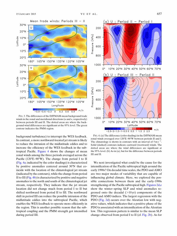
background turbulence) to interrupt the WES feedback.
In contrast, a more northward-located jet stream is likely
to reduce the intrusion of the midlatitude eddies and to
increase the efficiency of the WES feedback in the sub-
tropical Pacific. Figure 4 shows the changes of mean
zonal winds among the three periods averaged across the
Pacific (1208E–908W). The change from period I to II
(Fig. 4a; indicated by the color shadings) is characterized
by positive anomalies centered around 308N that co-
incide with the location of the climatological jet stream
(indicated by the contours), while the change fromperiod
II to III (Fig. 4b) is characterized by positive and negative
anomalies to the north and south of the climatological jet
stream, respectively. They indicate that the jet stream
location did not change much from period I to II but
shifted northward from period II to III. The northward
shift in period III can reduce the possible intrusion of the
midlatitude eddies into the subtropical Pacific, which
enables theWES feedback to operate more efficiently in
the region. This is another possible reason that the sub-
tropical coupling and the PMM strength got intensified
during period III.
We next investigated what could be the cause for the
intensification of the Pacific subtropical high around the
early 1990s?On decadal time scales, the PDOandAMO
are two major modes of variability that are capable of
influencing global climate. Here, we explored the pos-
sible connections between them and the early-1990s
strengthening of the Pacific subtropical high. Figures 2d,e
show the winter–spring SLP and wind anomalies re-
gressed onto the decadal (.10 yr) components of the
PDO and AMO indices. The largest regression with the
PDO (Fig. 2d) occurs over the Aleutian low with neg-
ative values, which indicates that a positive phase of the
PDO is associated with an intensification of theAleutian
low. This regression pattern is similar to the mean SLP
change observed from period I to II (cf. Fig. 2b). As for
FIG. 3. The differences of theDJFMAM-mean background trade
winds in the zonal and meridional directions (u and y, respectively)
between periods III and II. The dotted areas are where the back-
ground wind differences are significant at the 95% level. The green
contour indicates the PMM region.
FIG. 4. (a) The difference (color shading) in theDJFMAM-mean
zonal winds averaged over 1208E–908W between periods II and I.
The climatology is shown in contours with an interval of 5m s21.
Solid (dashed) contours indicate eastward (westward) winds. The
dotted areas are where the wind differences are significant at
the 95% level. (b) As in (a), but for the difference between periods
III and II.
15 JANUARY 2015 YU ET AL . 657
the AMO, the regressed SLP anomalies (Fig. 2e) are
largest in the regions of the Aleutian low and the sub-
tropical high with positive values. The regression in-
dicates that a positive phase of the AMO is associated
with a weakening of the Aleutian low and an intensi-
fication of the subtropical high. This regression pattern
is similar to the mean SLP change observed from
period II to III (cf. Fig. 2c). In particular, the SLP change
associated with the AMO also shows a clear northeast–
southwest orientation (highlighted by the red dashed
line in Fig. 2e) similar to the orientation of the SLP
changes in Fig. 2c. Therefore, the intensification of the
subtropical high during the early 1990s can be related to
a phase change of the AMO.
The linkage between the early-1990s strengthening of
the PMM intensity and the AMO can also be demon-
strated in Fig. 1b by adding the phase information for the
PDO and AMO into the figure. The figure shows that
the PDO switched from a negative phase (blue) to
a positive phase (red) around 1976, which is the year that
separates periods I and II. As for the AMO, its phase
switch occurred around 1995, which is close to the year
1993 that separates periods II and III. In period III, the
AMO switched to a positive phase, during which the
subtropical high should be intensified according to
the regression analysis (Fig. 2e). This analysis indicates
that the strengthening of the PMM intensity during the
early 1990s is closely linked to a phase change in the
AMO.As for the phase change of the PDOaround 1976,
it does not show a significant impact on the PMM in-
tensity. This is likely because the PDO phase change
primarily affects the strength of the Aleutian low, which
does not produce a strong impact on the subtropical
Pacific coupling.
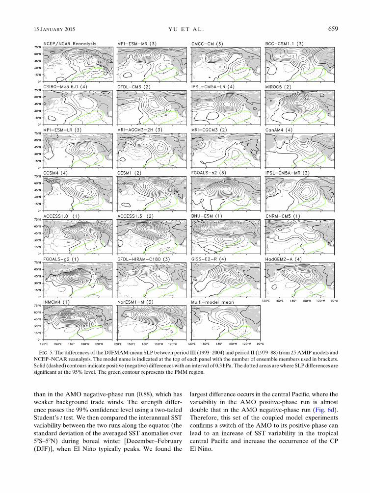
The possible influence of the AMO on the Pacific
subtropical high was further examined with 25 AMIP
model simulations, where observational SSTs are pre-
scribed from 1979 to 2010 to force AGCMs. Figure 5
shows the changes in the simulated mean SLPs between
periods III and II. During these two periods, the AMO
changed the phase from a negative to a positive in early
1990s while the PDO maintained its positive phase.
Therefore, the analysis of the model output can reveal
more concerning the influence of the AMO than that of
the PDO. To remove the possible contribution from
internal variability to the two-period difference, we used
the ensembles for each of the model simulations and
averaged across individual members of the same model.
We find from Fig. 5 that two AMIP models (MPI-ESM-
MRandCMCC-CM) produce distinct SLP changes near
Aleutian low and subtropical high that are very similar
to those found in observations. The next 13models (BCC-
CSM1.1 to IPSL-CM5A-MR) in the figure produce a
band of positive SLP differences extending from the
North Pacific to eastern subtropical Pacific. The positive
SLP differences in the subtropical Pacific penetrate well
into the PMM region enclosed by the green contours. The
last 10models (ACCESS1.0 toNorESM1-M) of the figure
simulate a similar pattern of the SLP differences to the
previous group of models but with smaller magnitudes of
SLP changes in the subtropical Pacific. Therefore, a ma-
jority (15 out of 25) of the AMIP models analyzed here
produces an intensification of the subtropical high from
period II to III. As indicated by the multimodel mean
shown in the last panel of Fig. 5, positive SLP changes
occur significantly in the subtropical Pacific (i.e., the west
of the Baja California) that extend southwestward (i.e.,
northeast–southwest orientation) to the tropical central
Pacific.Based on these results, it is reasonable to state that
the AMO intensification of the Pacific subtropical high
can be confirmed by AGCM simulations, although the
magnitude of the impact is underestimated.
Therefore, it is useful to couple an AGCM to a slab
ocean model to further examine the impact of the AMO
on tropical Pacific SST variability. We chose to use the
NCAR Community Atmospheric Model, version 3
(CAM3; Collins et al. 2006) coupled to a mixed-layer
slab ocean model for these experiments. Two experi-
ments were conducted: an AMO positive-phase run
and an AMO negative-phase run, in which SSTs cor-
responding to the positive and negative phases of the
AMO, respectively, were prescribed over the North
Atlantic (08–708N). SSTs in other regions were predicted
using the slab ocean model. The prescribed North At-
lantic SSTs were constructed by adding (subtracting)
SST anomalies associated with the positive (negative)
phase of the AMO to the climatological SSTs. The SST
anomalies are defined as the regressed SST pattern onto
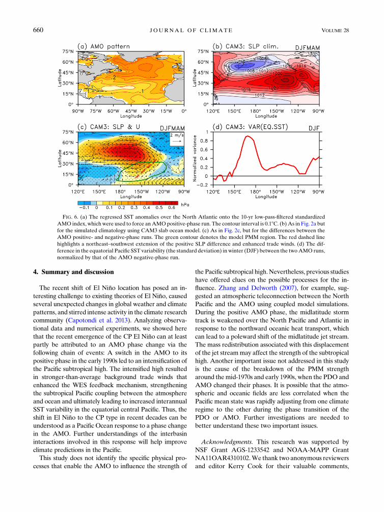
the AMO index (Fig. 6a) multiplied by a factor of 4. The
factor is used to insure that the model produces a strong
and clear enough response over the Pacific to the SST
forcing associated with the AMO. The model was in-
tegrated for 120 yr for each run and only the last 100 yr
were used for analysis.
Similar to most of the AMIP simulations, the SLP
differences between the two experiments (Fig. 6c) are
characterized by a band of positive values extending
from high latitudes in the central Pacific to the eastern
Pacific subtropics. It is encouraging that the northeast–
southwest extension of the positive SLP differences can
also be found in the eastern subtropical Pacific that co-
incides with the location of the PMM of the coupled
model. The PMM strength (i.e., the correlation co-
efficient between the PMM SST and wind indices) dur-
ing boreal spring is larger in the AMO positive-phase
run (0.94), which has stronger background trade winds,
658 JOURNAL OF CL IMATE VOLUME 28
than in the AMO negative-phase run (0.88), which has
weaker background trade winds. The strength differ-
ence passes the 99% confidence level using a two-tailed
Student’s t test. We then compared the interannual SST
variability between the two runs along the equator (the
standard deviation of the averaged SST anomalies over
58S–58N) during boreal winter [December–February
(DJF)], when El Niño typically peaks. We found the
largest difference occurs in the central Pacific, where thevariability in the AMO positive-phase run is almostdouble that in the AMO negative-phase run (Fig. 6d).Therefore, this set of the coupled model experiments
confirms a switch of the AMO to its positive phase can
lead to an increase of SST variability in the tropical
central Pacific and increase the occurrence of the CP
El Niño.
FIG. 5. The differences of the DJFMAM-mean SLP between period III (1993–2004) and period II (1979–88) from 25 AMIPmodels and
NCEP–NCAR reanalysis. The model name is indicated at the top of each panel with the number of ensemble members used in brackets.
Solid (dashed) contours indicate positive (negative) differences with an interval of 0.3 hPa. The dotted areas are where SLP differences are
significant at the 95% level. The green contour represents the PMM region.
15 JANUARY 2015 YU ET AL . 659
4. Summary and discussion
The recent shift of El Niño location has posed an in-teresting challenge to existing theories of El Niño, causedseveral unexpected changes in global weather and climatepatterns, and stirred intense activity in the climate researchcommunity (Capotondi et al. 2013). Analyzing observa-
tional data and numerical experiments, we showed here
that the recent emergence of the CP El Niño can at leastpartly be attributed to an AMO phase change via thefollowing chain of events: A switch in the AMO to itspositive phase in the early 1990s led to an intensification ofthe Pacific subtropical high. The intensified high resultedin stronger-than-average background trade winds thatenhanced the WES feedback mechanism, strengtheningthe subtropical Pacific coupling between the atmosphereand ocean and ultimately leading to increased interannualSST variability in the equatorial central Pacific. Thus, theshift in El Niño to the CP type in recent decades can beunderstood as a Pacific Ocean response to a phase changein the AMO. Further understandings of the interbasininteractions involved in this response will help improveclimate predictions in the Pacific.This study does not identify the specific physical pro-
cesses that enable the AMO to influence the strength of
the Pacific subtropical high.Nevertheless, previous studies
have offered clues on the possible processes for the in-
fluence. Zhang and Delworth (2007), for example, sug-
gested an atmospheric teleconnection between the North
Pacific and the AMO using coupled model simulations.
During the positive AMO phase, the midlatitude storm
track is weakened over the North Pacific and Atlantic in
response to the northward oceanic heat transport, which
can lead to a poleward shift of the midlatitude jet stream.
The mass redistribution associated with this displacement
of the jet streammay affect the strength of the subtropical
high. Another important issue not addressed in this study
is the cause of the breakdown of the PMM strength
around themid-1970s and early 1990s, when the PDOand
AMO changed their phases. It is possible that the atmo-
spheric and oceanic fields are less correlated when the
Pacific mean state was rapidly adjusting from one climate
regime to the other during the phase transition of the
PDO or AMO. Further investigations are needed to
better understand these two important issues.
Acknowledgments. This research was supported by
NSF Grant AGS-1233542 and NOAA-MAPP Grant
NA11OAR4310102.We thank two anonymous reviewers
and editor Kerry Cook for their valuable comments,
FIG. 6. (a) The regressed SST anomalies over the North Atlantic onto the 10-yr low-pass-filtered standardized
AMO index, which were used to force anAMOpositive-phase run. The contour interval is 0.18C. (b) As in Fig. 2a but
for the simulated climatology using CAM3 slab ocean model. (c) As in Fig. 2c, but for the differences between the
AMO positive- and negative-phase runs. The green contour denotes the model PMM region. The red dashed line
highlights a northeast–southwest extension of the positive SLP difference and enhanced trade winds. (d) The dif-
ference in the equatorial Pacific SST variability (the standard deviation) in winter (DJF) between the twoAMO runs,
normalized by that of the AMO negative-phase run.
660 JOURNAL OF CL IMATE VOLUME 28
Shang-Ping Xie of UCSD for the very helpful discussion
on the WES feedback mechanism, and Sang-Ki Lee of
NOAA for kindly providing us with the modified code
for CAM3. The NCEP–NCAR reanalysis, 20CR, and
ERSST datasets and the indices for the PDO and AMO
were downloaded from the NOAA/ESRL/PSD web ar-
chive (http://www.esrl.noaa.gov/psd) and JRA-55 data
are from theNCARCISLResearchDataArchive (http://
rda.ucar.edu/datasets/ds628.1). The AMIP model output
was obtained from the CMIP5 data archive (http://
pcmdi9.llnl.gov).
REFERENCES
Alexander, M., and Coauthors, 2006: Extratropical atmosphere–
ocean variability in CCSM3. J. Climate, 19, 2496–2525,
doi:10.1175/JCLI3743.1.
——, D. J. Vimont, P. Chang, and J. D. Scott, 2010: The impact
of extratropical atmospheric variability on ENSO: Testing
the seasonal footprinting mechanism using coupled model
experiments. J. Climate, 23, 2885–2901, doi:10.1175/
2010JCLI3205.1.
Anderson, B. T., 2003: Tropical Pacific sea-surface temperatures
and preceding sea level pressure anomalies in the subtropical
North Pacific. J. Geophys. Res., 108, 4732, doi:10.1029/
2003JD003805.
Ashok, K., S. Behera, A. S. Rao, H. Weng, and T. Yamagata, 2007:
El Niño Modoki and its teleconnection. J. Geophys. Res., 112,
C11007, doi:10.1029/2006JC003798.
Battisti, D. S., and A. C. Hirst, 1989: Interannual variability in the
tropical atmosphere–ocean model: Influence of the basic state,
ocean geometry and nonlinearity. J. Atmos. Sci., 46, 1687–1712,
doi:10.1175/1520-0469(1989)046,1687:IVIATA.2.0.CO;2.
Bretherton, C. S., C. Smith, and J. M. Wallace, 1992: An intercom-
parison of methods for finding coupled patterns in climate data.
J. Climate, 5, 541–560, doi:10.1175/1520-0442(1992)005,0541:
AIOMFF.2.0.CO;2.
Capotondi, A., and Coauthors, 2013: U.S. CLIVAR ENSO Di-
versity Workshop report. U.S. CLIVAR Rep. 2013-1, 23 pp.
Chang, P., L. Zhang, R. Saravanan, D. J. Vimont, J. C. H. Chiang,
L. Ji, H. Seidel, and M. K. Tippett, 2007: Pacific meridional
mode and El Niño–Southern Oscillation. Geophys. Res. Lett.,
34, L16608, doi:10.1029/2007GL030302.
Chiang, J. C. H., and D. J. Vimont, 2004: Analogous Pacific and
Atlantic meridional modes of tropical atmosphere–ocean
variability. J. Climate, 17, 4143–4158, doi:10.1175/JCLI4953.1.
Collins,W.D., andCoauthors, 2006: The formulation and atmospheric
simulation of the Community Atmosphere Model version 3
(CAM3). J. Climate, 19, 2144–2161, doi:10.1175/JCLI3760.1.
Compo, G. P., and P. D. Sardeshmukh, 2010: Removing ENSO-
related variations from the climate record. J. Climate, 23,1957–1978, doi:10.1175/2009JCLI2735.1.
——, and Coauthors, 2011: The Twentieth Century Reanalysis pro-
ject. Quart. J. Roy. Meteor. Soc., 137, 1–28, doi:10.1002/qj.776.
Czaja, A., P. van der Vaart, and J. Marshall, 2002: A diagnostic
study of the role of remote forcing in tropical Atlantic variability.
J.Climate, 15, 3280–3290, doi:10.1175/1520-0442(2002)015,3280:
ADSOTR.2.0.CO;2.
Ebita, A., and Coauthors, 2011: The Japanese 55-year Reanalysis
‘‘JRA-55’’: An interim report. SOLA, 7, 149–152, doi:10.2151/
sola.2011-038.
Enfield, D. B., A. M. Mestas-Nuñez, and P. J. Trimble, 2001: The
Atlantic multidecadal oscillation and its relation to rainfall
and river flows in the continental US. Geophys. Res. Lett., 28,
2077–2080, doi:10.1029/2000GL012745.
Gates, W. L., and Coauthors, 1999: An overview of the results
of the Atmospheric Model Intercomparison Project
(AMIP I). Bull. Amer. Meteor. Soc., 80, 29–55, doi:10.1175/
1520-0477(1999)080,0029:AOOTRO.2.0.CO;2.
Jin, F.-F., 1997: An equatorial recharge paradigm for ENSO. Part I:
Conceptual model. J. Atmos. Sci., 54, 811–829, doi:10.1175/
1520-0469(1997)054,0811:AEORPF.2.0.CO;2.
Kalnay, E., and Coauthors, 1996: The NCEP/NCAR 40-Year
Reanalysis Project. Bull. Amer. Meteor. Soc., 77, 437–471,
doi:10.1175/1520-0477(1996)077,0437:TNYRP.2.0.CO;2.
Kao, H.-Y., and J.-Y. Yu, 2009: Contrasting eastern Pacific and
central Pacific types of ENSO. J. Climate, 22, 615–632,
doi:10.1175/2008JCLI2309.1.
Kerr, R. A., 2000: A North Atlantic climate pacemaker for the cen-
turies.Science, 288, 1984–1986, doi:10.1126/science.288.5473.1984.Kim, S. T., J.-Y. Yu, A. Kumar, and H. Wang, 2012: Examination
of the two types of ENSO in the NCEP CFS model and its
extratropical associations. Mon. Wea. Rev., 140, 1908–1923,
doi:10.1175/MWR-D-11-00300.1.
Kug, J.-S., F.-F. Jin, and S.-I. An, 2009: Two types of El Niñoevents: Cold tongue El Niño and warm pool El Niño.J. Climate, 22, 1499–1515, doi:10.1175/2008JCLI2624.1.
Larkin, N. K., and D. E. Harrison, 2005: On the definition of El
Niño and associated seasonal averageU.S. weather anomalies.Geophys. Res. Lett., 32, L13705, doi:10.1029/2005GL022738.
Lee, T., and M. J. McPhaden, 2010: Increasing intensity of El Niñoin the central-equatorial Pacific. Geophys. Res. Lett., 37,
L14603, doi:10.1029/2010GL044007.
Lin, C.-Y., J.-Y. Yu, andH.H.Hsu, 2014: CMIP5model simulations
of the Pacific meridional mode and its connection to the two
types of ENSO. Int. J. Climatol., doi:10.1002/joc.4130, in press.
Mantua, N. J., S. R. Hare, Y. Zhang, J. M. Wallace, and R. C.
Francis, 1997: A Pacific decadal climate oscillation
with impacts on salmon production. Bull. Amer. Meteor.
Soc., 78, 1069–1079, doi:10.1175/1520-0477(1997)078,1069:
APICOW.2.0.CO;2.
McPhaden, M. J., T. Lee, and D. McClurg, 2011: El Niño and itsrelationship to changing background conditions in the tropicalPacific Ocean. Geophys. Res. Lett., 38, L15709, doi:10.1029/
2011GL048275.
Newman, M., S.-I. Shin, and M. A. Alexander, 2011: Natural var-
iation in ENSO flavors. Geophys. Res. Lett., 38, L14705,
doi:10.1029/2011GL047658.
Rogers, J. C., 1981: The North Pacific Oscillation. J. Climatol., 1,
39–57, doi:10.1002/joc.3370010106.
Schlesinger, M. E., and N. Ramankutty, 1994: An oscillation in the
global climate system of period 65-70 years. Nature, 367, 723–
726, doi:10.1038/367723a0.
Smith, T. M., R. W. Reynolds, T. C. Peterson, and J. Lawrimore,
2008: Improvements to NOAA’s historical merged land–
ocean surface temperature analysis (1880–2006). J. Climate,
21, 2283–2296, doi:10.1175/2007JCLI2100.1.Solomon, A., and M. Newman, 2012: Reconciling disparate
twentieth-century Indo-Pacific Ocean temperature trends in
the instrumental record. Nat. Climate Change, 2, 691–699,
doi:10.1038/nclimate1591.
Suarez, M. J., and P. S. Schopf, 1988: A delayed action oscillator
for ENSO. J. Atmos. Sci., 45, 3283–3287, doi:10.1175/
1520-0469(1988)045,3283:ADAOFE.2.0.CO;2.
15 JANUARY 2015 YU ET AL . 661
Taylor, K. E., R. J. Stouffer, andG.A.Meehl, 2012: An overview of
CMIP5 and the experiment design. Bull. Amer. Meteor. Soc.,
93, 485–498, doi:10.1175/BAMS-D-11-00094.1.
Vimont, D. J., D. S. Battisti, and A. C. Hirst, 2001: Footprinting:
A seasonal connection between the tropics and mid-
latitudes. Geophys. Res. Lett., 28, 3923–3926, doi:10.1029/
2001GL013435.
——, J. M. Wallace, and D. S. Battisti, 2003: The seasonal
footprintingmechanism in the Pacific: Implications for ENSO.
J. Climate, 16, 2668–2675, doi:10.1175/1520-0442(2003)016,2668:
TSFMIT.2.0.CO;2.
——, M. Alexander, and A. Fontaine, 2009: Midlatitude excitation
of tropical variability in the Pacific: The role of thermody-
namic coupling and seasonality. J. Climate, 22, 518–534,
doi:10.1175/2008JCLI2220.1.
Walker, G. T., and E. W. Bliss, 1932: World weather V. Mem.
R. Meteor. Soc., 4, 53–84.
Xie, S.-P., 1999: A dynamic ocean–atmosphere model of the
tropical Atlantic decadal variability. J. Climate, 12, 64–70,doi:10.1175/1520-0442-12.1.64.
——, and S. G. H. Philander, 1994: A coupled ocean-atmosphere
model of relevance to the ITCZ in the eastern Pacific. Tellus,
46A, 340–350, doi:10.1034/j.1600-0870.1994.t01-1-00001.x.Yeh, S. W., J. S. Kug, B. Dewitte, M. H. Kwon, B. P. Kirtman, and
F.-F. Jin, 2009: El Niño in a changing climate.Nature, 461, 511–
514, doi:10.1038/nature08316.
Yu, J.-Y., and H.-Y. Kao, 2007: Decadal changes of ENSO persis-
tence barrier in SST and ocean heat content indices: 1958-2001.
J. Geophys. Res., 112, D13106, doi:10.1029/2006JD007654.
——, and S. T. Kim, 2011: Relationships between extratropical sea
level pressure variations and the central Pacific and eastern
Pacific types of ENSO. J. Climate, 24, 708–720, doi:10.1175/
2010JCLI3688.1.
——, and B. S. Giese, 2013: ENSO diversity in observations.
CLIVAR Variations, Vol. 11, No. 2, U.S. CLIVAR, Wash-
ington, DC, 1–5.
——, H.-Y. Kao, and T. Lee, 2010: Subtropics-related inter-
annual sea surface temperature variability in the central
equatorial Pacific. J. Climate, 23, 2869–2884, doi:10.1175/
2010JCLI3171.1.
——, ——, ——, and S. T. Kim, 2011: Subsurface ocean tempera-
ture indices for central-Pacific and eastern-Pacific types of El
Niño and La Niña events. Theor. Appl. Climatol., 103, 337–
344, doi:10.1007/s00704-010-0307-6.
——, M.-M. Lu, and S. T. Kim, 2012: A change in the relationship
between tropical central Pacific SST variability and the ex-
tratropical atmosphere around 1990. Environ. Res. Lett., 7,
034025, doi:10.1088/1748-9326/7/3/034025.
Zhang, R., and T. L. Delworth, 2007: Impact of the Atlantic
multidecadal oscillation on North Pacific climate vari-
ability. Geophys. Res. Lett., 34, L23708, doi:10.1029/
2007GL031601.
662 JOURNAL OF CL IMATE VOLUME 28
Top Related