


Languages
Pages
Legal


Linear Systems of Equations
Direct Methods for Solving Linear Systems of Equations
Direct Methods for Solving Linear Systems of Equations
nnnnnnn
nn
nn
bxaxaxaE
bxaxaxaE
bxaxaxaE
2211
222221212
112121111
:
:
:
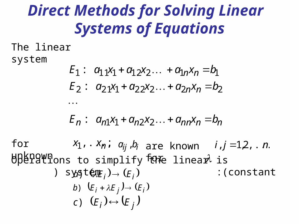
The linear system
iij ba ,for unknown
;,...,1 nxx are known for
nji ,...,2,1, Operations to simplify the linear system (
is constant:)
ii EEa )
iji EEEb )
ji EEc )
Direct Methods
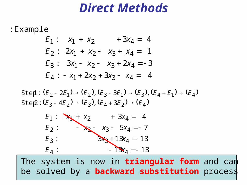
Example:
4 32 :
32 3 :
1 2 :
4 3 :
43214
43213
43212
4211
xxxxE
xxxxE
xxxxE
xxxE
3 ,4 :2 Step
,3 ,2 :1 Step
424323
414313212
EEEEEE
EEEEEEEEE
13 13 :
13 133 :
7 5 :
4 3 :
44
433
4322
4211
xE
xxE
xxxE
xxxE
The system is now in triangular form and can be solved by a backward substitution process

DefinitionsAn nxm (n by m) matrix:
ij
nmnn
m
m
a
aaa
aaa
aaa
A
. . .
. . .
21
22221
11211
The 1xn matrix (an n-dimensional row vector):
The nx1 matrix (an n-dimensional column vector):
x
.
. 2
1
nx
x
x
ynyyy 21
Definitions
A
nnnn
n
n
aaa
aaa
aaa
. . .
. . .
21
22221
11211
b
.
. 2
1
nb
b
b
bA,
:
. : . . .
. : . . .
:
:
21
222221
111211
nnnnn
n
n
baaa
baaa
baaa
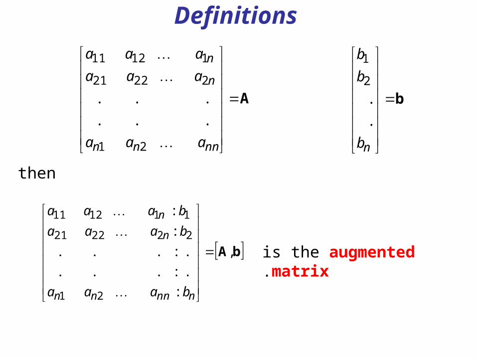
then
is the augmented matrix.
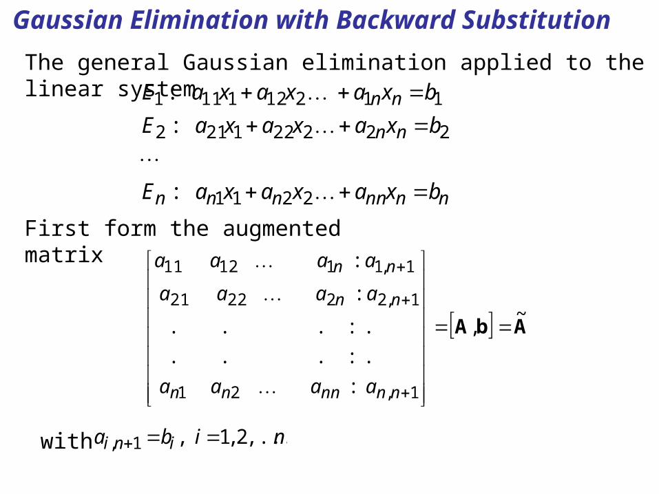
Gaussian Elimination with Backward Substitution
First form the augmented matrix
nnnnnnn
nn
nn
bxaxaxaE
bxaxaxaE
bxaxaxaE
2211
222221212
112121111
:
:
:The general Gaussian elimination applied to the linear system
AbA~
,
:
. : . . .
. : . . .
:
:
1,21
1,222221
1,111211
nnnnnn
nn
nn
aaaa
aaaa
aaaa
with niba ini ,...,2 ,1 ,1,

Gaussian Elimination with Backward Substitution
The procedure
....,,2,1 ,1,...,3 ,2each for / niijniEEaaE jiiijij
provided , yields the resulting matrix of the form
0iia
A~~
: 0........ .............0
. : . . .
. : . . .
: 0
:
1,
1,2222
1,111211
nnnn
nn
nn
aa
aaa
aaaa
which is triangular.

Gaussian Elimination (cont.)
Since the new linear system is triangular ,
,
.
.
1,
1,22222
1,11212111
nnnnn
nnn
nnn
axa
axaxa
axaxaxa
backward substitution can be performed
1 ,2 ,....,2 ,1 , 1
1,
nnia
xaa
xii
n
ijjijni
i when
.1,
nn
nnn a
ax

About Gaussian Elimination and Cramer’s Rule
Gaussian eliminations requires arithmetic operations.
)3/( 3nO
Cramer’s rule requires about arithmetic operations.
)!1( n
A simple problem with grid 11 x 11 involves n=81 unknowns, which needs operations.
1221075.4
What time is required to solve this problem by Cramer’s rule using 100 megaflops machine ?
101102.3 years !
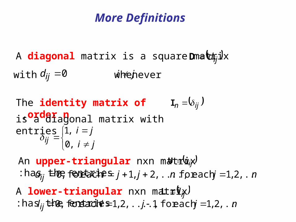
More Definitions
A diagonal matrix is a square matrix
with whenever
ijdD
0ijd ji
The identity matrix of order n ,
ijn I
is a diagonal matrix with entries
ji
jiij ,0
,1
An upper-triangular nxn matrix has the entries:
ijuU
njnjjiuij ,...,2 ,1each for ,....,2,1each for ,0
A lower-triangular nxn matrix has the entries:
ijlL
njjilij ,...,2 ,1each for 1,....,2 ,1each for ,0

Examples
D
3 0 0
0 2 0
0 0 1
U
0 0 0
5 0 0
3 2 0
U
6 0 0
5 4 0
3 2 1L
6 5 4
0 3 2
0 0 1
3
1 0 0
0 1 0
0 0 1
I
L
0 5 4
0 0 2
0 0 0
Do you see that ?AIAAI nn
Do you see that A can be decomposed as :
ULDA ?

Matrix Form for the Linear System
nnnnn
nn
nn
bxaxaxa
bxaxaxa
bxaxaxa
22211
22222121
11212111
The linear system
bAx
can be viewed as the matrix equation

LU decomposition
The factorization is particularly useful when it has the form
LUA
xyUxybLyUxLAxy
because we can rewrite the matrix equation bAx
Solving by forward substitution for y and then for x by backward substitution, we solve the
system .
bLy yUx

Matrix Factorization: LU decomposition
Theorem: If Gaussian elimination can be performed without row interchanges, then the decomposition A=LU is possible, where
U
nn
nn
n
u
u
u
uuu
0........... .....0
............. 0
.......
,1
22
11211
L
1 .....
.......0....................
...0..........0 1
..0.......... 0 0 1
1,n1
21
nnll
l
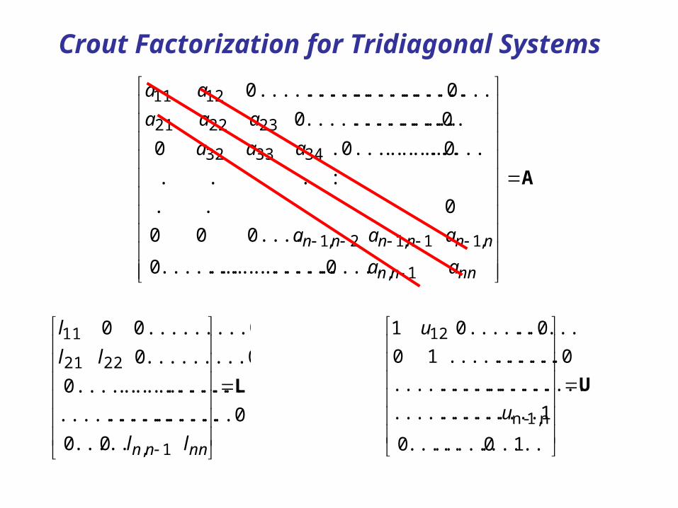
Crout Factorization for Tridiagonal Systems
A
nnnn
nnnnnn
aa
aaa
aaa
aaa
aa
0 ..................... .............0
0.... 0 0
0 . .
: . . .
0 ... ..........0........ 0
0 ... .........................0
0 ...................................... 0
1,
,11,12,1
343332
232221
1211
L
nnnn ll
ll
l
0 .....0
.......0....................
.................0.........
.........00
.........0 0 0
1,
2221
11
U
1 0........... .....0
.........1..........
.............................
......0.......... 1 0
..0.......... 0 1
n1,-n
12
u
u

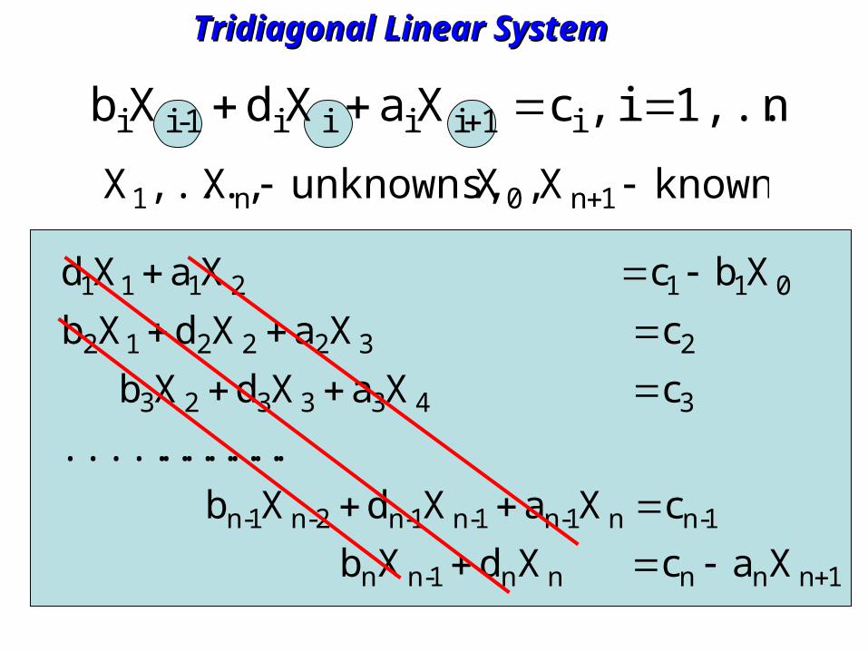
Tridiagonal Linear SystemTridiagonal Linear System
n1,...,i ,cXaXdXb i1iiii1-ii
known X,X unknowns, X,...,X 1n0n1
1nnnnn1-nn
1-nn1-n1-n1-n2-n1-n
3433323
2322212
0112111
Xac Xd Xb
c XaXdXb
................
c XaXdXb
c XaXdXb
Xbc XaXd

Tridiagonal Linear System: Tridiagonal Linear System: Thomas AlgorithmThomas Algorithm
Iterative Methods for Solving Linear Systems of Equations

Iterative Methods
And generate the sequence of approximation by
This procedure is similar to the fixed point method.
An iterative technique to solve Ax=b starts with an initial approximation and generates a sequence)0(x 0
)(k
kx
First we convert the system Ax=b into an equivalent formcTxx
...3,2,1 ,)1()( kkk cTxx
The stopping criterion:
)(
)1()(
k
kk
x
xx
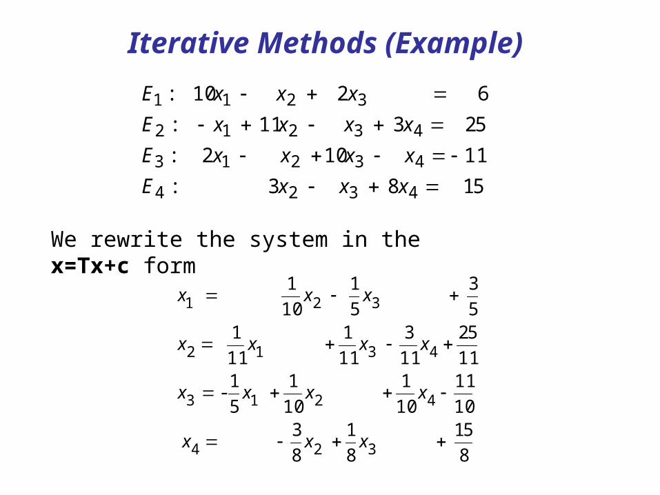
Iterative Methods (Example)
51 8 3 :
11 10 2 :
52 3 11 :
6 2 10 :
4324
43213
43212
3211
xxxE
xxxxE
xxxxE
xxxE
We rewrite the system in the x=Tx+c form
8
51
8
1
8
3
10
11
10
1
10
1
5
1-
11
52
11
3
11
1
11
1
5
3
5
1
10
1
324
4213
4312
321
xxx
xxxx
xxxx
xxx

Iterative Methods (Example) – cont.
1.8750 8
51
8
1
8
3-
1000.110
11
10
1
10
1
5
1-
2727.2 11
52
11
3 -
11
1
11
1
6000.0 5
3
5
1
10
1
)0(3
)0(2
)1(4
)0(4
)0(2
)0(1
)1(3
)0(4
)0(3
)0(1
)1(2
)0(3
)0(2
)1(1
xxx
xxxx
xxxx
xxx
and start iterations with
)0 ,0 ,0 ,0()0( x
Continuing the iterations, the results are in the Table:
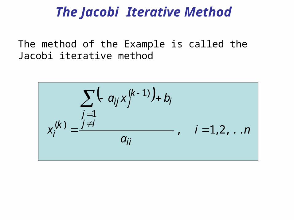
The Jacobi Iterative Method
The method of the Example is called the Jacobi iterative method
ni
a
bxa
xii
ijj
ikjij
ki ,....,2 ,1 ,
1
)1(
)(

Algorithm: Jacobi Iterative Method

The Jacobi Method: x=Tx+c Form
nnnn
n
n
aaa
aaa
aaa
. . .
. . .
21
22221
11211
A
ULD
0................... .....0
. ......................
.............................
................ 0
........ 0
0 .....
...........................
..........................
.........0..........
...0.......... ............. 0
..0...............0
.......0....................
............................
...0.......... 0
.....0..........0
n1,-n
2
112
1,1
2122
11
a
a
aa
aa
a
a
a
a
n
n
nnnnn
ULDA

The Jacobi Method: x=Tx+c Form (cont)
ULDA and the equation Ax=b can be transformed into
bxULD
bxULDx
bDxULDx 11
ULDT 1 bDc 1Finally

The Gauss-Seidel Iterative Method
8
51
8
1
8
3-
10
11
10
1
10
1
5
1-
11
52
11
3 -
11
1
11
1
5
3
5
1
10
1
)(3
)(2
)(4
)1(4
)(2
)(1
)(3
)1(4
)1(3
)(1
)(2
)1(3
)1(2
)(1
kkk
kkkk
kkkk
kkk
xxx
xxxx
xxxx
xxx
The idea of GS is to compute using most recently calculated values. In our example:
)(kx
Starting iterations with , we obtain
)0 ,0 ,0 ,0()0( x

The Gauss-Seidel Iterative Method
ni
a
bxaxa
xii
i
j
n
iji
kjij
kjij
ki ,....,2 ,1 ,
1
1 1
)1()(
)(
Gauss-Seidel in form (the Fixed Point)
cTxx )1()( kk
bUxxLD
bxULDAx )(
bUxxLD )1()( kk
cT
bLDxULDx 1)1(1)( kkFinally

Algorithm: Gauss-Seidel Iterative Method

The Successive Over-Relaxation Method (SOR)
)1()()( )-(1 ki
ki
ki xxx
The SOR is devised by applying extrapolation to the GS metod. The extrapolation tales the form of a weighted average between the previous iterate and the computed GS iterate successively for each component
where denotes a GS iterate and ω is the extrapolation factor. The idea is to choose a value of ω that will accelerate the rate of convergence.
)(kix
10 under-relaxation21 over-relaxation

SOR: Example
244
30 4 3
42 3 4
32
321
21
xx
xxx
xx
Solution: x=(3, 4, -5)
Top Related