


Languages
Pages
Legal

Charlotte Hamilton, Caressa Mainland, Jacob Morgan, Chris Tiller
Linear Algebra
Dr. McClain
12/12/14
Population Growth and the Leslie Matrix
For our project, we used a Leslie matrix to look at a population of haddock fish and their
future population projections. Haddock fish are a staple of the New England fishing industry, an
area that provides over 80% of the fish we eat in the United States. In the 20th century, as our diet
grows to include more fish, it’s important to study the lifetimes of fish and the effect of netting
and pollution in their areas. We used a Leslie matrix to estimate and project future populations.
A Leslie matrix is a type of matrix that is used for population projects by recording the
birth rate and survival rate of each age of fish. We were given this matrix:
Haddock live ten years and each column represents an age group. The first row shows the
birth rate of each age group and the diagonals show the survival rate of each age group. To find a
projected population, you multiply the Leslie matrix by the population vector, each row
representing an age group of fish. Unfortunately, that will only give you a projection of the next
year. To find the projection of years further in the future, you raise the Leslie matrix to the
number of years in the future you’d like to project.
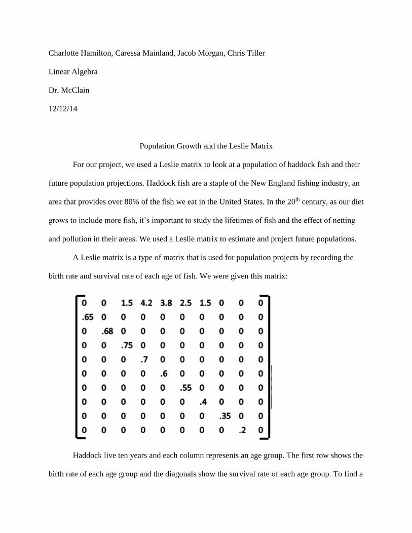
For part one of our project we are asked, “If the haddock population in 1900 is
(100,0,0,0,0,0,0,0,0,0)t (units are millions of pounds), what will the population be like in 1910?
1920? 1930? 1950? 1995? 2000? Based upon what you have seen, do you believe the population
to be stable or unstable?” This information is displayed in our matrices:

Judging from this information we can infer that the population is unstable, because it’s
growing exponentially. It doesn’t hit a point where it plateaus, it just continues to grow. This is
what we expect, however, with no effects such as predation, harvesting, or pollution acting on
the population; with the fish only dying of old age, it makes sense that there would only be a
very large increase in population over time.
So because we think the population is unstable, we are then asked, “If you believe it to be
unstable, pick two consecutive populations where the ratios of all components (cohorts) are
approximately constant. What is that constant? What does it tell you about the long term
behavior of the system?”
Looking at our matrices, 1900 and 1910 aren’t usable matrices for this process because
they contain 0s and will therefore not yield a proper ratio. 1920 and beyond however are fair
game. This process is fairly simple: to begin, I looked for a pattern. I isolated the closest sets of
data chronologically that we found earlier, 1995 and 2000, and noticed that each value in 1995
appeared to be multiplied by roughly four to reach the value in 2000. However, these are not
immediately consecutive populations. They are a good lead nevertheless.
I applied the same logic by comparing the matrices of 1921 and 1920. I took the first
value of 1921 and divided it by the corresponding value in 1920. The result was 1.32. This gives
us the ratio 1:1.32, or basically for every one fish we have in the previous matrix, there will be
1.32 fish in the subsequent matrix. I multiplied each member of the 1920 matrix by 1.32 and

obtained a matrix that looked nearly identical to our computed 1921 matrix.
I decided to repeat this process on a consecutive pair of years much later in our data;
1995 and 1996. When I repeated the process, the same ratio was obtained and consistent
throughout the matrices. This leads me to believe that the population of haddock is multiplying at
a rate of 1.32 yearly, which is clearly not stable since it’s a rate of constant increase. What we
can infer from this data is a point that was hit on earlier: left to only natural death, a population
of fish will reproduce extremely quickly.
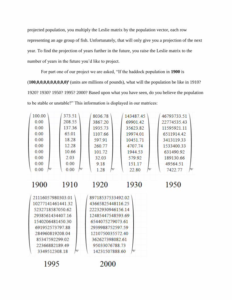
In part two of Fishing in George’s Bank, we are asked to consider an environmental
effect that changes the birth rates and survival rates of our fish population between the years
1950 and 1990. With the effects of pollution on the fish, their birth rates and survival rates are
decreased by 10% and 15% respectively. Once after this data has been collected, we will
compare that to the population of fish that has been unaffected by the pollution to determine the
consequences. Below will be both of the matrices used in this part.
Original Leslie Matrix
[
0 0 1.5 4.2 3.8 2.5 1.5 0 0 00.65 0 0 0 0 0 0 0 0 00 0.68 0 0 0 0 0 0 0 00 0 0.75 0 0 0 0 0 0 00 0 0 0.7 0 0 0 0 0 00 0 0 0 0.6 0 0 0 0 00 0 0 0 0 0.55 0 0 0 00 0 0 0 0 0 0.4 0 0 00 0 0 0 0 0 0 0.35 0 00 0 0 0 0 0 0 0 0.2 0]
Leslie Matrix with Pollution
[
0 0 1.4 4.1 3.7 2.4 1.4 0 0 00.5 0 0 0 0 0 0 0 0 00 0.53 0 0 0 0 0 0 0 00 0 0.6 0 0 0 0 0 0 00 0 0 0.55 0 0 0 0 0 00 0 0 0 0.45 0 0 0 0 00 0 0 0 0 0.40 0 0 0 00 0 0 0 0 0 0.25 0 0 00 0 0 0 0 0 0 0.2 0 00 0 0 0 0 0 0 0 0.05 0]
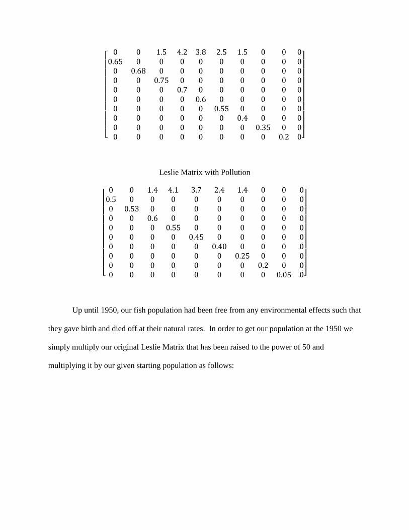
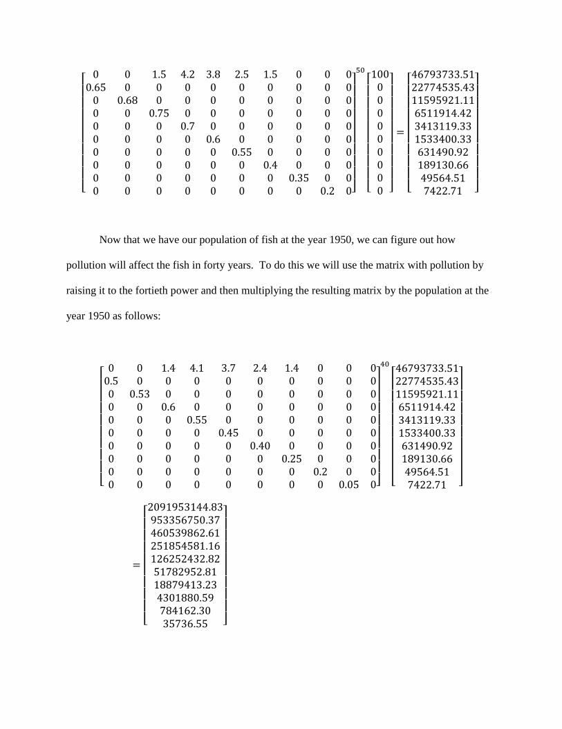
Up until 1950, our fish population had been free from any environmental effects such that
they gave birth and died off at their natural rates. In order to get our population at the 1950 we
simply multiply our original Leslie Matrix that has been raised to the power of 50 and
multiplying it by our given starting population as follows:
[
0 0 1.5 4.2 3.8 2.5 1.5 0 0 00.65 0 0 0 0 0 0 0 0 00 0.68 0 0 0 0 0 0 0 00 0 0.75 0 0 0 0 0 0 00 0 0 0.7 0 0 0 0 0 00 0 0 0 0.6 0 0 0 0 00 0 0 0 0 0.55 0 0 0 00 0 0 0 0 0 0.4 0 0 00 0 0 0 0 0 0 0.35 0 00 0 0 0 0 0 0 0 0.2 0]
50
[ 100000000000 ]
=
[ 46793733.5122774535.4311595921.116511914.423413119.331533400.33631490.92189130.6649564.517422.71 ]
Now that we have our population of fish at the year 1950, we can figure out how
pollution will affect the fish in forty years. To do this we will use the matrix with pollution by
raising it to the fortieth power and then multiplying the resulting matrix by the population at the
year 1950 as follows:
[
0 0 1.4 4.1 3.7 2.4 1.4 0 0 00.5 0 0 0 0 0 0 0 0 00 0.53 0 0 0 0 0 0 0 00 0 0.6 0 0 0 0 0 0 00 0 0 0.55 0 0 0 0 0 00 0 0 0 0.45 0 0 0 0 00 0 0 0 0 0.40 0 0 0 00 0 0 0 0 0 0.25 0 0 00 0 0 0 0 0 0 0.2 0 00 0 0 0 0 0 0 0 0.05 0]
40
[ 46793733.5122774535.4311595921.116511914.423413119.331533400.33631490.92189130.6649564.517422.71 ]
=
[ 2091953144.83953356750.37460539862.61251854581.16126252432.8251782952.8118879413.234301880.59784162.3035736.55 ]

Now, to compare our data between fish that have been exposed to pollution and fish that
have not. To get the population for our fish from 1900 to 1990, follow the above example on
getting the population of fish from 1900 to 1950, but raise the matrix to the ninetieth power.
With that, the comparison is shown below:
[ 4969852573424.442418816901859.241231566988441.81691616641604.64362501332054.55162857209602.5367068070275.2720087317026.885264245207.02788337595.66 ]
[ 2091953144.83953356750.37460539862.61251854581.16126252432.8251782952.8118879413.234301880.59784162.3035736.55 ]
Without Pollution With Pollution
From this data, it is clearly seen that over a forty year time frame, pollution has been able
to put a dent in the fish population. Taking the first age group, the numbers reduced from
4.9 ∗ 1012 to 2.09 ∗ 109. The same hit can be seen every other age group.
For the third part of our project, we wanted to consider ways of reigning in the
population. Although pollution helped to limit the growth, harvesting is another viable option.
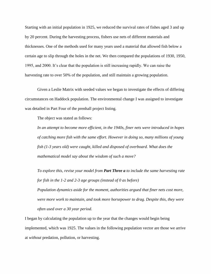
Starting with an initial population in 1925, we reduced the survival rates of fishes aged 3 and up
by 20 percent. During the harvesting process, fishers use nets of different materials and
thicknesses. One of the methods used for many years used a material that allowed fish below a
certain age to slip through the holes in the net. We then compared the populations of 1930, 1950,
1995, and 2000. It’s clear that the population is still increasing rapidly. We can raise the
harvesting rate to over 50% of the population, and still maintain a growing population.
Given a Leslie Matrix with seeded values we began to investigate the effects of differing
circumstances on Haddock population. The environmental change I was assigned to investigate
was detailed in Part Four of the prenhall project listing.
The object was stated as follows:
In an attempt to become more efficient, in the 1940s, finer nets were introduced in hopes
of catching more fish with the same effort. However in doing so, many millions of young
fish (1-3 years old) were caught, killed and disposed of overboard. What does the
mathematical model say about the wisdom of such a move?
To explore this, revise your model from Part Three a to include the same harvesting rate
for fish in the 1-2 and 2-3 age groups (instead of 0 as before)
Population dynamics aside for the moment, authorities argued that finer nets cost more,
were more work to maintain, and took more horsepower to drag. Despite this, they were
often used over a 30 year period.
I began by calculating the population up to the year that the changes would begin being
implemented, which was 1925. The values in the following population vector are those we arrive
at without predation, pollution, or harvesting.

Taking this a step further the values in the matrix below are those that we find once we begin to
factor in harvesting and death rate changes. These changes occur during the year 1925.
This is now the update death rate Leslie Matrix and we are applying the population vector given
to us from M25*PopVec1. We are raising the harvestMatrix to the power of the number of years
we need to account for, from the time that it is valid, until the time we are wanting to consider
PopVec1940Harvest = ((HarvestMatrix^15)*PopVector);
Hence below is the population vector for the year 1940, having factored in pollution and
harvesting of the haddock population.
The Leslie matrix had to be modified once to reflect the
changes we were to consider.
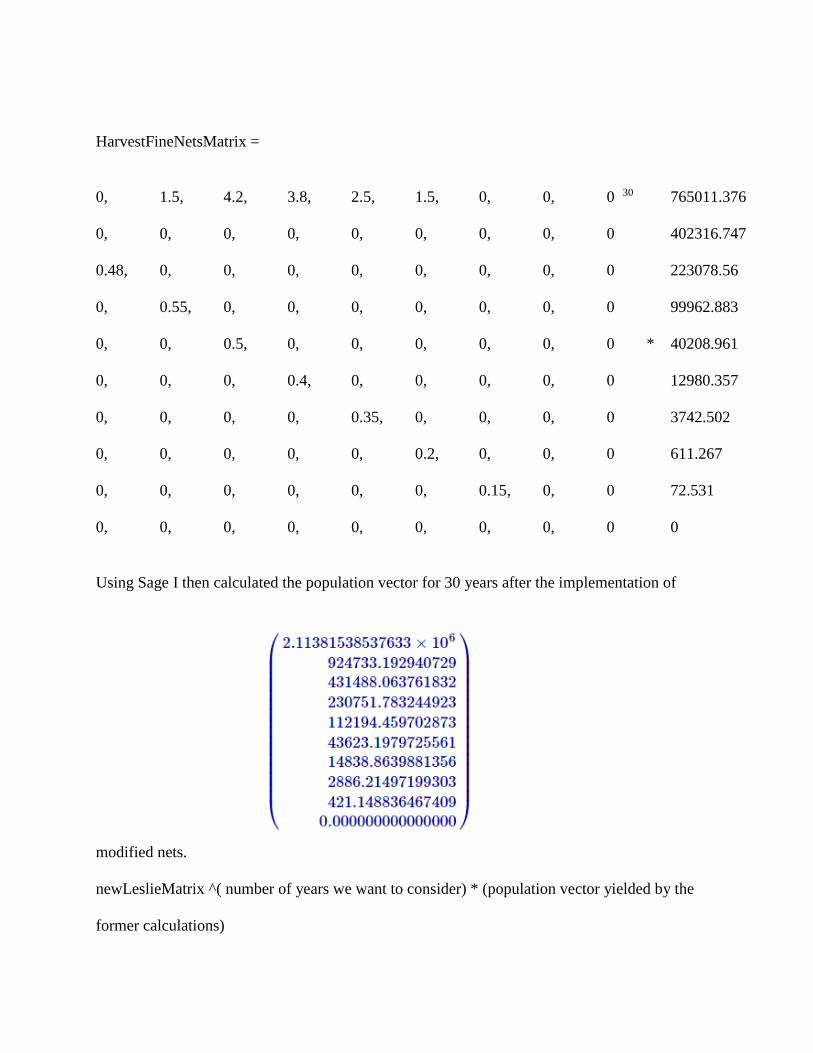
HarvestFineNetsMatrix =
0, 1.5, 4.2, 3.8, 2.5, 1.5, 0, 0, 0 30 765011.376
2.114* 106
0, 0, 0, 0, 0, 0, 0, 0, 0 402316.747
924733.193
0.48, 0, 0, 0, 0, 0, 0, 0, 0 223078.56
431488.064
0, 0.55, 0, 0, 0, 0, 0, 0, 0 99962.883
230751.783
0, 0, 0.5, 0, 0, 0, 0, 0, 0 * 40208.961
112194.46
0, 0, 0, 0.4, 0, 0, 0, 0, 0 12980.357
43623.198
0, 0, 0, 0, 0.35, 0, 0, 0, 0 3742.502
14838.864
0, 0, 0, 0, 0, 0.2, 0, 0, 0 611.267
2886.215
0, 0, 0, 0, 0, 0, 0.15, 0, 0 72.531
421.149
0, 0, 0, 0, 0, 0, 0, 0, 0 0
0
Using Sage I then calculated the population vector for 30 years after the implementation of
modified nets.
newLeslieMatrix ^( number of years we want to consider) * (population vector yielded by the
former calculations)

FineNetPopVector = ((HarvestFineNetsMatrix^30)*PopVec1940Harvest);
This needs to be compared to the populations that are considered stable, we need to examine if
the trend were to continue and consider whether or not this leads to a stable population.
I again used the same method and calculation to assess the population impacts both 50
and 100 years after implementation.
Year 50:
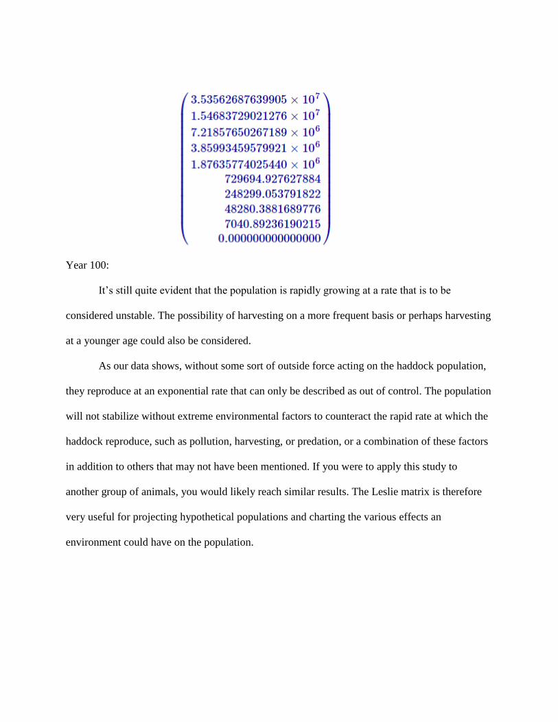
Year 100:
It’s still quite evident that the population is rapidly growing at a rate that is to be
considered unstable. The possibility of harvesting on a more frequent basis or perhaps harvesting
at a younger age could also be considered.
As our data shows, without some sort of outside force acting on the haddock population,
they reproduce at an exponential rate that can only be described as out of control. The population
will not stabilize without extreme environmental factors to counteract the rapid rate at which the
haddock reproduce, such as pollution, harvesting, or predation, or a combination of these factors
in addition to others that may not have been mentioned. If you were to apply this study to
another group of animals, you would likely reach similar results. The Leslie matrix is therefore
very useful for projecting hypothetical populations and charting the various effects an
environment could have on the population.
Top Related