


Languages
Pages
Legal


University of Southern Queensland
Faculty of Engineering and Surveying
Life Cycle Assessment of a Personal Computer
A dissertation submitted by
Baipaki Pakson Hikwama
in fulfillment of the requests of
Courses ENG4111 and 4112 Research Project
towards the degree of
Bachelor of Engineering (Electrical & Electronics)
Submitted: October, 2005
ii
Abstract
This research project aims to assess the components parts of a PC to determine which
parts contribute most adverse to environmental impacts, and to make recommendations
about the potential for recycling and recovery of materials at the end-of-life of a PC. The
investigation is performed by implementing LCA methodology on the PC. This paper
summarizes the methodology generated. A PC used is the Pentium IV ABA PC including
the Compaq monitor, keyboard and mouse. The procedure of the LCA follows the ISO
14040 series. System boundary includes the entire life cycle of the product, including raw
material acquisition, material processing, transportation, use and disposal. The LCI and
impact database for a PC is constructed using SimaPro software version 6.0 after
disassembling the PC and taking an inventory of its component parts.
The results of the study show that the production and the use stages are the most
contributing phases. In the production phase, PC manufacturing consists of simple
processes such as assembly and packaging. Assembly processes of the computer parts
such as PCB assembly, CRT assembly, and ICs assembly are the most contributing in this
phase. The use stage has a significant potential due to electricity consumption. The
disposal stage s contribution is very small in comparison. Possible ways of improving the
environmental burden, such as reduction of power consumption of the PC, are also
outlined in this paper. This paper concludes by outlining the main achievements and
some future work of this project.

iii
University of Southern Queensland
Faculty of Engineering and Surveying
ENG4111 & ENG4112 Research Project
Limitations of Use
The Council of the University of Southern Queensland, its Faculty of Engineering and Surveying, and the staff of the University of Southern Queensland, do not accept any responsibility for the truth, accuracy or completeness of material contained within or associated with this dissertation.
Persons using all or any part of this material do so at their own risk, and not at the risk of the Council of the University of Southern Queensland, its Faculty of Engineering and Surveying or the staff of the University of Southern Queensland.
This dissertation reports an educational exercise and has no purpose or validity beyond this exercise. The sole purpose of the course pair entitled "Research Project" is to contribute to the overall education within the student s chosen degree program. This document, the associated hardware, software, drawings, and other material set out in the associated appendices should not be used for any other purpose: if they are so used, it is entirely at the risk of the user.
Prof G Baker Dean Faculty of Engineering and Surveying

iv
Certification
I certify that the ideas, designs and experimental work, results, analyses and conclusions set out in this dissertation are entirely my own effort, except where otherwise indicated and acknowledged.
I further certify that the work is original and has not been previously submitted for assessment in any other course or institution, except where specifically stated.
Baipaki Pakson Hikwama
Student Number: 0031132340
_____________________________________ Signature
_____________________________________ Date

v
Acknowledgements
To carry out a research of this nature, and to express it in a written form is only possible
through the support, assistance and supervision of patient, caring and loving people.
First of all, I express my appreciation to Mr. David Parsons who was patient and open in
guiding and supporting me throughout the duration of my project. My thanks also go to
the technical staff especially Terry and Brett for their technical assistance. Finally, I
would like to also thank my friends Marina Smith and Jorja Forster for their help and
support; not only for the achievement of this piece of work, but in life in general. Without
their understanding, the work of this dissertation would not have reached the deadlines.

vi
Contents
Title Page i
Abstract ii
Disclaimer Page iii
Certification Page iv
Acknowledgements v
Table of Contents vi
List of Figures viii
List of Tables xi
1. Introduction 1
1.1 Outline of the report 3
2. Life Cycle Assessment 4
2.1 Background Information of LCA 4
2.2 The Components of LCA 5
2.2.1 Goal and Scope 5
2.2.2 Life Cycle Inventory 5
2.2.3 Life Cycle impact Assessment 6
2.2.4 Interpretation 6
2.3 LCA Standards 7
2.4 Types of LCA 7
2.4.1 Conceptual 7
2.4.2 Simplified LCA 8
2.4.3 Detailed LCA 8
2.5 Literature 8
3. Project Methodology 10
3.1 How the Methodology was Conducted 10
3.1.1 Product Composition Data 11

vii
3.1.2 Production Stage Data 11
3.1.3 Distribution Stage Data 11
3.1.4 Use Stage Data 12
3.1.5 Disposal Stage Data 12
3.2 LCA Methodology with SimaPro 12
3.2.1 Damage to Human Health 13
3.2.2 Damage to Ecosystem Quality 14
3.2.3 Damage to Resources 15
4. Goal and Scope of the Project 17
4.1 Goal of this Project 17
4.2 Scope of the Project 17
4.2.1 Product and Functional Unit 17
4.2.2.1 The Structure of a Personal Computer 18
4.2.2 System Boundaries 20
4.3 Using Thresholds in SimaPro 22
4.4 Allocation 22
5. Life Cycle Inventory 24
5.1 Disassembly of the PC 24
5.2 Calculation of the Environmental Load 36
5.2.1 Description of Life Stages 37
5.2.1.1 Production of Raw Materials 38
5.2.1.2 Manufacturing 38
5.2.1.3 Distribution 38
5.2.1.4 Use 39
5.2.1.5 Disposal 39
6. Life Cycle Impact Assessment 41
6.1 Validation of Eco-indicator 99 Methodology 44
6.2 Results and Discussion from the Inventory Analysis 45
6.3 Results and Discussion from the Impact Assessment 47
6.3.1 The Whole PC 48
6.3.1.1 Normalization 56

viii
6.3.1.2 Damage Assessment 57
6.3.2 Control Unit 59
6.3.3 CRT Monitor 68
6.3.4 Relative Contributions of the PC Elements 76
6.4 Discussion of Overall Results 78
7. Conclusions and Recommendations 80
7.1 Main Achievements of Objectives 80
7.2 Future Work 82
8. List of References 83
9. Bibliography 85
10. Appendix A: Project Specification 87
11. Appendix B: LCI Input/Output Tables 88
11.1 The Whole PC 88
11.2 Control Unit 104
11.3 CRT Monitor 117
12. Appendix C: Material Composition of a Personal Computer 133

ix
List of Figures
Figure 3-1: General representation of the Eco-indicator methodology 16
Figure 4-1: Life Cycle Stages of a Computer 21
Figure 5-1A: The motherboard and daughterboard of a PC 25
Figure 5-1B: The disassembled hard disk drive (HDD) 25
Figure 5-1C: The disassembled floppy disk drive (FDD) 26
Figure 5-1D: Power supply of a PC system pulled apart 27
Figure 5-1E: CD-ROM drive of a PC disassembled 28
Figure 5-1F: The desktop cabinet of a PC 29
Figure 5-1G: Data cables and the mains cables from a PC system 29
Figure 5-2A: The printed board with some components pulled off 32
Figure 5-2B: Internal Components of a CRT Monitor 33
Figure 5-3A: The different parts of a keyboard 35
Figure 5-4A: All the parts in a PC mouse 36
Figure 5-5A: The model of the life cycle of a PC from raw materials to disposal 37
Figure 6-1A: Consumption of resources in life cycle of a PC (minerals). 45
Figure 6-1B: Consumption of fossil fuel resources in the life cycle of a PC 46
Figure 6-1C: Environmental emissions in the life cycle of a PC 47
Figure 6-2A: Characterization results of the environmental impact of whole PC system 48
Figure 6-2B: Characterized network showing aspects of PC life cycle and relative
use of fossil fuels 50
Figure 6-2C: Characterized network showing the aspect of climate change (global warming) as a
result of the life cycle of a PC 51
Figure 6-2D: Characterized network shows aspects of PC life cycle and resource consumption
(use of mineral resources) 52
Figure 6-2E: Network shows aspects of PC life cycle and relative contributions to respiratory in-
organics 53
Figure 6-2F: Characterization network of acidification/eutrophication 54
Figure 6-2G: Characterization network on the results on eco-toxicity in the life
cycle of a PC 55
Figure 6-2H: Normalization of environmental impact potentials of the whole PC 57
Figure 6-2I: Damage assessment of the life cycle of a PC on a single score 58

x
Figure 6-2J: Normalized damage category results 58
Figure 6-2K: Damage assessment results of the PC life cycle on a weighted scale 59
Figure 6-3A: shows the characterized results of the environmental impacts for the
Control Unit 60
Figure 6-3B: shows the characterized effects of global warming due to climate
change caused by the control unit 61
Figure 6-3C: shows the aspects of the control unit life cycle and the relative use
of fossil fuels (resources) 62
Figure 6-3D: Characterized results of mineral resources potential due to the
Control Unit life cycle 63
Figure 6-3E: Characterization results of acidification/eutrophication index in
the life cycle for the control unit 64
Figure 6-3F: Normalized environmental potentials for control unit 65
Figure 6-3G: The normalized damage categories for the control unit 66
Figure 6-3H: The weighted damage assessment results Control unit lifecycle 67
Figure 6-3I: damage assessment for the control unit on a single score 68
Figure 6-4A: Characterized environmental impact potential - CRT monitor 69
Figure 6-4B: Characterized results showing aspects of the CRT monitor life cycle
and effect on climate change 70
Figure 6-4C: Characterized results of acidification/eutrophication index for the monitor 71
Figure 6-4D: Aspects of the life cycle of the CRT monitor and relative use of fossil fuels 72
Figure 6-4E: Characterized mineral resources index for the life cycle of the CRT monitor 73
Figure 6-4F: Normalized damage assessment for CRT monitor life cycle 74
Figure 6-4G: Weighting of the damage assessment for the CRT monitor life cycle 75
Figure 6-4H: Damage assessment of the life cycle for the CRT monitor on a single score 76
Figure 12-1: Material composition of a personal computer 134

xi
List of Tables
Table 1: Direct and Indirect Effect of providing $1 million dollar of products in the
Computer/Office Equipment 2
Table 5-1A: Parts and Materials in the Control Unit 30
Table 5-1B: Parts and Weights in the Monitor 34
Table 5-1C: Parts and Weights in the Keyboard 35
Table 5-1D: Parts and Weights in the PC mouse 36
Table 6-1A: Classifications of Emissions to Air 42
Table 6-1B: Environmental Impact categories 43
Table 6-1C: Contribution to Environmental Impact Potential, PC by Element 76
Table 6-1D: contributions to Damage, PC by Element 77
Table 11-1A: Damage Assessment to Ecosystem Quality in the PC system 88
Table 11-1B: Damage Assessment to Human Resources for the PC system 90
Table 11-1C: Damage Assessment to Resources for the Whole PC system 94
Table 11-1D: Characterized Climate Change for the Whole PC 97
Table 11-1E: Characterization results of fossil fuels for the Whole PC 98
Table 11-1F: Characterization results of Eco-toxicity in the Whole PC 100
Table 11-1G: Characterization results for Acidification/Eutrophication in the PC system 101
Table 11-1H: Characterization of consumption of mineral resources 101
Table 11-1I: Characterization of respiratory effects (in-organics) 102
Table 11-1J: Characterized environmental impacts of a PC per impact category 103
Table 11-1K: Normalization of environmental load of a PC per impact category 103
Table 11-1L: Weighted environmental load of a PC per impact category 103
Table 11-1M: Damage Assessment Results of the Whole PC 104
Table 11-1N: Normalized Damage Assessment of the PC system 104
Table 11-1O: Weighting of Damage Assessment Results of the PC 104
Table 11-2A: Damage Assessment to Ecosystem Quality 104
Table 11-2B: Damage Assessment to Human Health 106
Table 11-2C: Damage Assessment to Resources 109
Table 11-2D: Characterized Climate Change, the Control Unit 111
Table 11-2E: Characterized Fossil Fuels, Control Unit 112
Table 11-2F: Characterization of Mineral resources, Control Unit 114
Table 11-2G: Characterized Respiratory Effects (in-organics) Control Unit 114

xii
Table 11-2H: Characterized Environmental Load - Control Unit 115
Table 11-2I: Normalized Environmental Load per Impact Category - Control Unit 115
Table 11-2J: Weighted Environmental Load per Impact Category - Control Unit 116
Table 11-2K: Damage Assessment Results for the Control Unit 116
Table 11-2L: Normalized Damage Assessment for the Control Unit 116
Table 11-2M: Weighting of Damage Assessment for the Control Unit 116
Table 11-3A: Damage Assessment to Ecosystem Quality 117
Table 11-3B: Damage Assessment to Human Health 119
Table 11-3C: Damage Assessment to Resources 123
Table 11-3D: Characterized mineral resources 125
Table 11-3E: Characterized Climate Change CRT Monitor 125
Table 11-3F: Characterized results on the use of fossil fuels 126
Table 11-3G: Characterized Results on the Extraction of Mineral Resources 128
Table 11-3H: Characterized Eco-toxicity CRT Monitor 129
Table 11-3I: Characterized Acidification/Eutrophication CRT Monitor 129
Table 11-3J: Characterized Respiratory Effects (in-organics) CRT Monitor 130
Table 11-3K: Characterized Environmental Load per impact category - CRT Monitor 130
Table 11-3L: Normalized Environmental Load per Impact Category 131
Table 11-3M: Weighting Environmental Load per Impact Category CRT Monitor 131
Table 11-3N: Damage Assessment Results CRT Monitor 131
Table 11-3O: Normalized Damage Assessment for the CRT Monitor 131
Table 11-3P: Damage Assessment on a weighted scale CRT Monitor 132
Table 12-1: Product Composition in 17-inch CRT Monitor 133

1
CHAPTER 1
Introduction
Electric and electronic goods constitute one of the fastest growing categories of consumer
goods in the world today (US EPA 1999). Often being the very symbols of material
welfare, they have become intimately connected to our modern way of life and several
have become indispensable everyday aids. More so, computer technology has had a
substantial impact on the development of several technological and scientific disciplines,
besides the field of communication itself. One of these disciplines is the modeling of
complex meteorological and climatic patterns in the earth s atmosphere, crucial for our
understanding of our own human impact on the climate, which is heavily dependent on
powerful computer technology. The modern communication society would not be what
it is today without the aid of advanced electronic appliances.
Apart from the importance of these products in facilitating modern life, and being
important tools to combat today s environmental and societal problems, they also bring
about significant health and environmental hazards. The PC, of which this project
focuses, is no exception. Some of these aspects, such as solvent releases, hazardous waste
generation and water and energy consumption, occur as a result of production processes,
whereas others, such as the emission of electromagnetic radiation and consumption of
energy, occur during the use phase of the products. Still others, related to end-of-life
treatment, occur due to the product content. Examples of the latter are the occurrence of
halogenated flame retardants and toxic metals in PC components. With new substances
continuously being incorporated into the products and with the volumes of personal
computers entering the market each year ever increasing, new health and environmental
aspects are occurring and are likely to continue to do so.
According to Matthews (2003, p.1760), little attention is placed upon the potential
environmental impacts of Information and Communications Technology (ICT) around
the world. These negative environmental impacts arise from among others, a globally-

2
polluting supply chain and from producing the electricity needed to power computers.
Table 1 below gives an approximate value of the environmental impact of
Computer/Office Equipment in USA in 1997 by Matthews (2003). The direct component
is defined as the environmental effect that can be attributed directly to an industry s
operations, while the indirect component results from a corresponding change in demand
for all other industries in the economy associated with the supply chain for an industry.
Table 1: Direct and Indirect Effects of providing $1 million of products in the
Computer/Office Equipment (US, 1997)
Computer/Office Equipment
Effects Units Total Direct Indirect
Electricity used 106 kW-hr 0.436 0.093 0.343
Energy used Terajoule 8.5 0.275 8.225
Conventional pollutants
released
Metric tons 6.838 0.057 6.781
Fatalities Lives 0.001 0.000 0.001
CO2 equivalent gases
released
Metric tons 585 13 572
Hazardous waste
generated
Metric tons 39 25 14
Toxic releases and
transfers
Metric tons 0.939 0.039 0.9
Weighted toxic releases Metric tons 7.712 0.093 7.619
From the table the most effects generally occur from indirect purchases in the supply
chain. The energy used to produce $1 million of computers is approx. 97% in the indirect
purchases.

3
Matthews (2003, p.1762) furthers says this about electronic devices:
Most electronic devices consume power even when turned off, because they leak energy in
standby and sleep modes. They also generate heat which must be dissipated by ventilation
(of which this is an indirect source of electricity demand).
Hence this project aims to analyze a PC specifically in more detail. This is done by the
use of life cycle assessment (LCA) methods which are incorporated into the SimaPro
software. Further analyses is conducted on which of the PC parts contribute most to
adverse environmental impacts of the whole PC system. The results obtained will be
compared to previous studies that have been conducted on the same product, such as
Life Cycle Assessment; An Approach to Environmentally Friendly PCs by Tekwawa et
al. (1997).
1.1 Outline of the project
Chapter 2 covers the background and literature of LCA, and further summarizes the four
components of a LCA study. Chapter 3 provides an introduction to the methodology used
in this study and some current technologies associated with SimaPro software as well as a
short review of the studies that have been done on a particular PC. Chapter 4 covers the
goal and scope of this project in more detail. In Chapter 5, an overview of the system
description and its lifecycle inventory is given. Chapter 6 contains the central analysis of
the project, that is, the lifecycle inventory (LCI) is categorized and characterized as
potential environmental impacts. The results of the environmental load are given and
discussed in this chapter. Ways of reducing some potential impacts are also discussed in
here. In Chapter 7 some conclusions on what is being achieved and future work is
provided here. Chapter 8 gives some details of the study in the form of Appendices.
Appendix A presents a copy of the Project Specification, and Appendix B presents
detailed input/output data from the LCI.

4
CHAPTER 2
Life Cycle Assessment
2.1 Background Information of LCA
Life cycle assessment (LCA) is the calculation and evaluation of the environmentally
relevant inputs and outputs, and the potential environmental impacts of the life cycle of a
product, material or service (ISO, 1997). Environmental inputs & outputs refer to demand
for natural resources, and to emissions and solid waste.
LCAs evaluate the environmental impacts from each of the following major life cycle
stages, raw material acquisition; material processing; transport; product manufacture;
product use; and final disposition (ISO 14040). All processes start with the extraction of
raw materials and energy from the environment. They proceed through the stages of
production and consumption. And they end with disposal, when the product may be
transported to a municipal waste treatment plant where it is dismantled. Parts of the
product may be recovered for recycling and other parts are incinerated. Thus disposal
also involves several processes which require materials, energy and services. Ultimately,
all material inputs from the environment are transformed by economic processes and re-
enter the environment as emissions to water, air and land. LCA is sometimes called a
cradle-to-grave assessment.

5
2.2 The Components of LCA
LCA generally has four components (ISO 1997). These include:
(i) Defining the goal and scope of the study.
(ii) Making a model of the product life cycle with all environmental inflows
and outflows. This data collection effort is usually referred to as the life-
cycle inventory (LCI) stage.
(iii) Understanding the environmental relevance of all inflows and outflows;
this is referred to as the life-cycle impact assessment (LCIA) phase.
(iv) The interpretation of the study.
2.2.1 Goal and Scope
The goal and scope definition is the first step in a LCA study. In this phase the purpose of
the study is described. This description includes the intended application and audience,
and reasons for carrying out the study (Udo de Haes et al. 2002, p.1). Furthermore, the
scope of the study is described. This includes a description of the limitations of the study,
the functions of the systems investigated, the functional unit, the systems investigated,
the system boundaries, the allocation approaches, the data requirements, data quality
requirements, the key assumptions, the impact assessment method, the interpretation
method, and the type of reporting.
2.2.2 Life Cycle Inventory
The main technique used in LCA is that of modeling. In the inventory phase, a model is
made of the complex technical system that is used to produce, transport use and dispose
of a product. This results in a flow sheet or process tree with all the relevant processes.
For each process, all the relevant inflows and the outflows are collected. Emissions,

6
energy requirements and material flows are calculated for each process. These data will
then be adapted and/or weighted to the functional unit, which is defined in the goal and
scope, so that the whole life cycle of the product can be taken into account (Pre
Consultants, 2002).
2.2.3 Life Cycle Impact Assessment
Life-cycle impact assessment (LCIA) is the process in which the input and the output
data from an LCI are aggregated across all life cycle stages and translated into impacts
and examined from an environmental perspective using category indicators (Udo de Haes
et. 2002, p.2). In the life cycle impact assessment phase, a completely different model is
used to describe the relevance of inflows and outflows. For this, a model of an
environmental mechanism is used. For example, an emission of SO2 could result in an
increased acidity, which can cause changes in soils that result in dying trees, etc
(Goedkoop & Oele 2004). By using several environmental mechanisms, the LCI result
can be translated into a number of impact categories such as acidification, climate
changes etc. The LCIA also provides information for the interpretation phase.
According to ISO (International Organization for Standardization 14040 series (1997,
2000), life-cycle impact assessment (LCIA) consists of two mandatory elements,
classification and characterization, and three optional elements, normalization, grouping,
and weighting.
2.2.4 Interpretation
The Life Cycle Interpretation is the phase where the results are analyzed in relation to the
scope definition, where conclusions are reached, the limitations of the results are
presented and where recommendations are provided based on the findings of the
preceding phases of the LCA.

7
2.3 LCA Standards
LCA approaches are generally guided by standards; and from a standard perspective they
are dealt with under the umbrella of the ISO 14000 series. The main documents are as
follows:
ISO 14040
Life Cycle Assessment
General principles, framework and
requirements for the LCA of products and services (1997)
ISO 14041 Life Cycle Inventory analysis (1998)
ISO 14042 Life Cycle Impact Assessment (2000)
ISO 14043 Life Cycle Interpretation (2000)
2.4 Types of LCA
There are three different types of LCA. They are conceptual, simplified and detailed
LCA. According to UNEP (1996), these three different types can be used in different
ways depending upon the context in which they are used.
2.4.1 Conceptual LCA
The conceptual LCA is the simplest form of LCA and is used at a very basic level to
make an assessment of environmental aspects, based upon a limited and usually
qualitative inventory. The results of a conceptual LCA can usually be presented using
qualitative statements, graphics, flow diagrams or simple scoring systems which indicate
which components or materials have the largest environmental impacts and why.

8
2.4.2 Simplified LCA
Simplified LCA applies the LCA method for screening assessment (i.e. covering the
whole life cycle). Screening is made using already available data or estimated data that is
already in the database (Goedkoop & Oele 2004). For missing data, provisional
alternatives are taken. For example, if you need nickel production, and you only have
data on some other non-ferro metals, you use these alternatives to get an impression of
the importance of this process.
2.4.3 Detailed LCA
Detailed LCAs involve the full process of undertaking LCAs and require extensive and
in-depth data collection, specifically focused upon the target of the LCA, which if only
available generically, must be collected specifically on the product or service under
review.
Of the three types of LCA discussed, simplified (screening) is used in this study.
2.5 Literature
The energy crises in the 1970s and the resource depletion concerns raised by publications
such as Limits to Growth (Meadows, et al., 1972) set a trend where more thought
began to be given to ways and means of optimizing resource usage. Rising energy costs
triggered the need for more systematic and detailed energy usage planning. (UNEP-IE,
1996) LCA was developed in parallel to energy planning initiatives and the need for
detailed energy analyses within it.
During the 1980s a growing focus upon global warming and resource depletion
influenced an increased interest in LCA. This was accompanied by more LCA studies

9
being made available publicly. It was at this stage that databases began to be developed to
meet the complex inventory and assessment data needs of the studies.
A confusing situation arose towards the end of the 1980s when environmental reports on
similar products often contained conflicting results because they were based on different
methods, data and terminology. It soon became clear that there was a need for
standardization in environmental reporting. Hence by 1997, the first LCA standard was
developed, ISO 14040, which deals with principles and framework of LCA.
Today, knowledge of how to carry out an LCA is improving rapidly. The value of the
technique is being increasingly recognized and it is now being used for strategic decision
making and for designing environmental policies.

10
CHAPTER 3
Project Methodology
The methodology of the project involved a study of the literature and background
information to develop an understanding of the current LCA technology and its
associated standards, as well as an understanding of the current methodology associated
with SimaPro and its usage. To analyze and assess the environmental impacts of a PC, a
few things were carried out, that is, a particular PC was disassembled and an inventory of
its components parts was constructed. Weights of the different parts of the computer,
together with packaging were also taken, to aggregate the total weight of the PC. Then
measurements of energy consumption were taken from a typical similar PC under a
variety of conditions (i.e. when the monitor is on and the control unit and keyboard off;
when control unit and keyboard on but monitor off; and when control unit and keyboard
and monitor are all on). A model of the lifecycle of the PC from raw material to ultimate
disposal was further constructed. Then various analyses using SimaPro software were
performed. The broad analysis of LCA performed by the software incorporates
categories such as human health, ecosystem quality and natural resource use etc into the
impact assessment. The analyses were further supported by a study of relevant literature
for comparison of results to similar products.
3.1 How the Methodology was conducted
This is how the methodology was carried out in detail. First, data was prepared for the
different stages of the life cycle of a PC. Data prepared were product composition data;
production stage data; distribution stage data; use stage data; and the disposal stage data.

11
3.1.1 Product Composition Data
The PC that is being evaluated in this study is a desktop PC that comprises a cathode ray
tube (CRT) monitor, control unit, keyboard and mouse. The monitor is a Compaq and the
control unit is an ABA model, both of which were manufactured in early 1997 in
Malaysia, Asia. To prepare the product composition data, the desktop PC was
disassembled into components such as the hard disk drive (HDD), floppy disk drive
(FDD), CD-ROM drive, power supply, etc, and the weight of each component was
measured. The components were further dismantled, and the weight and number of the
materials in them determined. Tabulated results for the disassembled PC are in chapter 5.
3.1.2 Production Stage Data
The production stage data comprised parts manufacturing, material manufacturing and
the assembly processes. Most of the background data such as fuels, aluminum sheet,
copper sheet, packaging materials, glass, electricity, emissions, energy, waste
management, materials production, transport, etc, are readily available in LCA databases
such as SimaPro software.
The inventory data for electronic parts such as semiconductor devices, resistors,
capacitors, transformers and coils, printed circuit boards, and cables were obtained after
disassembling the PC, and from LCA reports on similar product such as Life Cycle
Assessment; An Approach to Environmentally Friendly PCs, by Tekawa M, etal., 1996 .
3.1.3 Distribution Stage Data
Distribution stage data were obtained by assuming the PC is transported from Malaysia to
Brisbane by ship; and from Brisbane to Toowoomba by a 28-ton truck; and from
Toowoomba wholesale to University of Southern Queensland (USQ) by a delivery van.

12
The carrying capacity of each transportation stage was obtained by multiplying the
distance traveled by the weight of the PC. For example, the distance from Malaysia to
Brisbane is approx. 6000km, and the weight of the PC is approx. 29kg (0.029 tonnes),
therefore the carrying capacity of the ship for this PC is about 174tkm.
3.1.4 Use Stage Data
The power consumption for the PC was measured. The computer s life was assumed to
be 5 years, being operated 8hrs/day and 240days/year. Hence the use stage data for this
PC was calculated by multiplying the power consumption by the operating time. More
detail on the use stage is on section 5.2.
3.1.5 Disposal Stage Data
The disposal stage data were obtained assuming that 30% of the used products from PCs
are recycled; and that 70% of the used products from PCs are broken into fragments and
landfilled.
3.2 LCA Methodology with SimaPro
The main technique used in LCA is that of modeling. In the inventory phase, a model is
made of the complex technical system that is used to produce, transport, use and dispose
of a product. This results in a flow sheet or process tree with all the relevant processes.
For each process, all the relevant inflows and the outflows are collected. The result is
usually a long list of inflows and outflows that is often difficult to interpret. In the life
cycle impact assessment phase, a completely different model is used to describe the
relevance of inflows and outflows. For this, a model of an environmental mechanism is

13
used. For example, SO2, could result in an increased acidity, increased acidity can cause
changes in soils that result in dying trees, etc.
So the inventory data for each life cycle stage including the product composition data
were input into SimaPro and a life cycle inventory and impact analysis for the desktop
PC was conducted. The impact assessment method used is Eco-indicator 99 (E) V2.1
Australian substances. The impact analysis categories analyzed were climate change
(which is often called global warming), resource consumption (which includes minerals
and fossil fuels), respiratory effects (in-organics), acidification/eutrophication, land use,
carcinogens, eco-toxicity and respiratory effects (organics).
There are three types of environmental damages associated with this methodology:
Human Health
Ecosystem Quality
Resources
A detailed description of each damage category is given below:
3.2.1 The Damage to Human Health
The health of any human individual, being a member of the present or a future
generation, may be damaged either by reducing its duration of life by a premature death,
or by causing a temporary or permanent reduction of body function (disabilities).
According to the current knowledge, the environmental sources for such damages are
mainly the following:
Infectious diseases, cardiovascular and respiratory diseases, as well as forced
displacement due to the climate change.
Cancer as a result of ionizing radiation.
Cancer and eye damage due to ozone layer depletion.

14
Respiratory diseases and cancer due to toxic chemicals in air, drinking water and
food.
These damages represent the most important damages to human health caused by
emissions from product systems. To aggregate different types of damages to human
health, the DALY (Disability Adjusted Life Years) scale is used. The core of the DALY
is a disability weighting scale. The scale lists many different disabilities on a scale
between 0 and 1 (0 meaning being perfectly health and 1 meaning death).
Example: Carcinogenic substances cause a number of deaths each year. In the DALY
health scale, death has a disability rating of 1. If a type of cancer is (on average) fatal ten
years prior to the normal life expectancy, we would count 10 lost life years for each case.
This means that each case has a value of 10 DALYs.
3.2.2 The Damage to Ecosystem Quality
The species diversity is used as an indicator for ecosystem quality. This damage category
is expressed as a percentage of species that are threatened or disappear from a given area
during a certain time due to environmental load. Impact categories associated with this
damage category are explained in the following paragraph:
- Eco-toxicity is expressed as the percentage of all species present in the
environment living under toxic stress (PAF Potentially Affected Fraction).
- Acidification and eutrophication are treated as a single score. Here the damage
to target species (vascular plants) in natural areas is modeled.
- Land use and land transformation is based on empirical of the occurrence of
vascular plants as a function of the land-use type and the area size. Both the
local damage on the occupied or transformed area as well as the regional
damage on ecosystems is taken into account.

15
The unit for damages to Ecosystem Quality is the PDF times area affected times years on
which this applies [PDF*m2.yr], where PDF stands for potentially disappeared fraction.
3.2.3 The Damage to Resources
In Eco-indicator 99 methodology, only mineral resources and fossil fuels are modeled. In
this category the concentration of a resource is the main element of resource quality. That
is, as more minerals are extracted, the energy requirements for future mining will
increase. The damage is the energy needed to extract a kg of a mineral in the future. For
fossil fuels the concept of surplus energy is used.
The unit of resources damage category is the surplus energy in MJ per kg extracted
material. This is the expected increase of extraction energy per kg extracted material
when mankind has extracted an amount that is N times the cumulative extracted materials
since the beginning of extraction. Surplus energy is used to add the damages from
extracting different resources.
Figure 3-1 below, which is taken from Goedkoop and Spriensma (2001), gives a general
representation of the Eco-indicator methodology as used in LCA databases such as
SimaPro software. A limiting assumption is that in principle all emissions and land uses
are occurring in Europe and that all subsequent damages occur in Europe; except for the
damages to resources and the damages created by climate change, ozone layer depletion,
air emissions of persistent carcinogenic substances, inorganic air pollutants that have
long-range dispersion, and some radioactive substances.

16
Damage to minerals & fossil resources [MJ surplus energy]
Damage to ecosystem quality [% Vascular plant species*km2*yr]
Damage to human health [disability adjusted life years (DALY)].
Surplus energy for future extraction
Conc. SPM and VOCs
Local effect on vascular plant species
Surplus energy for future extraction
Regional effect on vasc. plant species
Acid/eutro (occurrence target species)
Ozone layer depletion (cancer)
Ecotoxicity:toxic stress (PAF)
Climate change (diseases & displace)
Carcinogenesis (cancer cases & type)
Respiratory effects (cases & type)
Ion. radiation (cancer cases & type)
Changed pH &nutrient avail.
Change in habitat size
Fossil fuel avail. (per type)
Concentration minerals
Conc. ozone depletion gases
Conc. greenhouse gases
Conc. urban,agric, natural soil
Indicator
Conc. radionuclides
Extraction of minerals and fossil fuels
Conc. in air, water, food
Damage analysis
Land-use: occupation & transformation
NOX
SOX
NH3
Pesticides Heavy metals CO2
HCFC Nuclides (Bq) SPM VOCs PAHs
Resource analysis Land-use analysis Fate analysis
Exposure and Effect analysis
Normalization and weighting
Figure 3-1: General representation of the Eco-indicator methodology. The boxes at the bottom of the figure (those with block arrows on top) refer to procedures; while the other boxes refer to intermediate results.

17
CHAPTER 4
Goal and Scope of the Project
4.1 Goal of this project
The goal of this project is to identify and assess the most significant environmental
impacts of a personal computer through a lifecycle inventory analysis (LCI) and impact
assessment. This includes having to disassemble a particular PC and construct a life cycle
inventory of its component parts; to construct a model of the lifecycle of particular PC
from raw material to ultimate disposal, and hence determine which parts contribute most
adverse environmental impacts. The LCA technologies analysis provide the opportunity
to use the model as a stepping stone for further analyses and improvement assessments
for this personal computer.
4.2 Scope of the project
Scope is defined by the system boundaries, the functional unit (which is the structure of
the personal computer) and input/output species. These are described in the following
subsections.
4.2.1 Product and Functional Unit
The product system being analyzed in this study is a standard personal computer with
five years of lifetime. Though the technical lifetime of the computer may be longer than
five years, the USQ ITS keeps them for service for 5 years. The product system includes
the central processing unit (CPU) or control unit, a CRT monitor, keyboard and a mouse.

18
In an LCA, product systems are evaluated on a functionally equivalent basis. The
functional unit is used as the basis for the inventory and impact assessment to provide a
reference to which the inputs and outputs are related.
4.2.1.1 The structure of a personal computer (functional unit)
A standard, modern personal computer is comprised of four different units; the control
unit (CU), the visual display unit (VDU), which is the CRT monitor, the keyboard and
the mouse. Brief overviews of the different sections of the personal computer are outlined
below.
The Control Unit
The control unit (CU) is the central unit of a PC; this is where information is processed
and stored. The CU contains the motherboard on which are mounted the electronic
circuits necessary for the functioning of the computer. The most central part of the CU is
the processor circuit, which is the brain of the computer, directing all the information
flows between the different parts of the computer. Mounted on the motherboard are
graphical cards, and working memory or RAM (Random Access Memory) as it is also
called.
All these units consist predominantly of transistors made from semi-conducting
materials, mainly silicon. The motherboard is what is called a printed wiring board (a
laminated plate with electric circuits) on which is mounted semiconductor components.
The memory units of the CU can be divided into working memory and the disc
memories. The RAM is a temporary storage place, intimately connected to the processor,
for information being used when the PC is in the on-mode . When the computer is shut
down the RAM is emptied. The disc memories, on the other hand, are permanent storage
facilities for information. There are three main types of disc memories two based on

19
magnetic technology, the hard disc and the floppy disc, and one using optical technology,
the CD-ROM. The hard disc is permanently installed in the CU and has the highest
storage capacity, while the other two are inserted temporarily into special disc drive units.
Mouse and Keyboard
The mouse and the keyboard are both tools to transform external information into a form
that can be stored in either of the PC s memory units. That is, they are both input
devices .
Both mouse and keyboard basically contain plastics and a few electronic circuits to
transfer the information provided by the PC operator. Thus they contain no parts that
differ significantly in production related environmental aspects from the CU.
The Visual Display Unit
The VDU is, on the other hand, an output device . This is where information is
presented to the operator in an understandable fashion. In this project the type of VDU
assessed is the cathode ray tube (CRT) monitor. This uses the same technology as the
traditional TV set, i.e., a current of electrons creates an image on a glass panel, projected
by electric and magnetic fields.

20
4.2.2 System Boundaries
Since a model of the lifecycle of a PC is constructed from raw material to ultimate
disposal, the boundaries of this study are where raw materials are extracted from the
ground/environment; emissions to ambient air occur from operations, after treatment;
residual wastes are landfilled, with exception of wastewater emissions from landfills,
which are included for metals. The product system studied is scoped to focus on relevant
impact categories as defined in SimaPro, from direct production, transport, use and
disposal operations that comprise the life cycle. Figure 1-1 briefly describes each of the
stages for a computer product system. The inputs (e.g., resources and energy) and outputs
(e.g., product and waste within each life cycle stage, as well as the interaction between
each stage (e.g., transportation) are evaluated to determine the environmental impacts.

21
INPUTS LIFE-CYCLE STAGES OUTPUTS
RAW MATERIALS EXTRACTION
Activities related to the acquisition of natural
resources, including mining non-renewable material,
harvesting biomass, and transporting raw materials to
processing facilities.
MATERIALS PROCESSING
Processing natural resources by reaction, separation,
purification, and alteration steps in preparation for the
manufacturing stage; and transporting processed
materials to product manufacturing facilities.
PRODUCT MANUFACTURE
Processing materials and assembling components parts
to make a computer (that is, control unit, CRT monitor,
keyboard and the mouse).
PRODUCT USE, MAINTENANCE, AND REPAIR
Computers are transported to and used by customers.
Maintenance and repair may be conducted either at the
customer s location or taken back to a service center or
manufacturing facility.
Materials
Energy
Resources
FINAL DISPOSITION
At the end of its useful life, the computer is retired. If
reuse and recycle of usable parts is feasible, the product
can be transported to an appropriate facility and
disassembled. Parts and materials that are not
recoverable are then transported to appropriate
facilities and treated (if required or necessary) and/or
disposed of.
Wastes
Products
Figure 4-1: Life cycle stages of a computer
(Source: http://www.epa.gov/dfe/pubs/comp-dic/lca)

22
4.3 Using thresholds in SimaPro
Many inventories apply so-called cut-off rules, whereby those individual inputs that
constitute very small percentages of total inputs to the system are ignored. The effect of
using cut-off criteria can be analyzed in the process tree or network window in SimaPro.
In many LCAs process trees become very large, up to about 2000 processes. Some of
these processes do not contribute much to the load. To illustrate this, a cut-off threshold
can be set for displaying processes in the process tree at any percentage, say, 2.2%, and
0.5%, of the environmental load (for a single score or an impact category). In most cases
only a few processes turn out to have a contribution that is above the threshold. In this
project, no cut-off rules have been applied, that is, an attempt has been made to represent
the entire life cycle of the system. For some inputs where emissions/energy data is
unavailable, an assumption has been used, usually the closest analogous process for
which data are available.
4.4 Allocation
Many processes usually perform more than one function or output. The environmental
load of that process needs to be allocated over different functions and outputs. In general,
the best solution to allocation is to avoid it in the first place. In SimaPro each process can
have multiple outputs and avoided outputs at the same time. This means you can combine
system boundary expansion and direct allocation in a way that best suit your project. For
most unit operations in the system, the generally accepted convention of allocating
resource consumptions and emissions according to the proportional mass of the
economically useful products has been applied. For instance, if a process s output is 20
kg of A, 20 kg of B, A and B each are credited with half of the emissions. That is, for
each multiple output, you can add a percentage that indicates the allocation share.

23
In the use phase, allocation is assumed in such a way that the personal computer is
operated 8 hours a day, 240 days a year for 5 years. The power consumption rate for this
computer was tested for a similar typical PC.
In the disposal stage, it is assumed that 70% and 30% of the used products from the PC
are landfilled and recycled respectively. In the waste management of this PC, the large
assemblies such as cathode ray tube (CRT), printed circuit boards (PCBs), cabinet, power
cords, cables are assumed to be manually separated at the end of the product life cycle,
and then recycled. The packaging materials such as cardboard, plastic inserts, foam are
usually recycled. Other components such as electrical cables, cable clamp, etc are
landfilled.

24
CHAPTER 5
Life Cycle Inventory
This chapter contains a summary of the pollutants emitted and resources consumed in
delivering, using and disposing of a personal computer. The goal, scope and methodology
that has already been outlined in the preceding chapters, show that the life-cycle
inventory of a personal computer has been compiled.
To generate the inventory, a particular PC was disassembled, its components parts
constructed into an inventory and its life-cycle described.
5.1 Disassembly of the PC
As already mentioned in the preceding chapters, the personal computer consists of four
main parts; control unit, monitor, keyboard and mouse. The different subparts and their
weights are shown in the next tables. For the printed circuit boards with components,
weights for different components in the board were taken and hence the weight of the
PCB with components aggregated, except for the electrolytic capacitors, choking coils
and transformers which were excluded from the weight of the printed circuit board with
components.
Table 5-1A shows different parts and weights of the control unit. The motherboard
consists of the motherboard PCI, the Cache RAM, controller port, printed circuit board
(PCB) with components for the CPU and the BUS-print plus for the cooling body for the
CPU.

25
Figure 5-1A: shows the motherboard and the daughter board of the PC
The hard disk drive consists of a cover, casing, hard disk plate and printed circuit board (PCB) with components as shown in figure 5-1B. The hard disk plate is assumed to be made from alloyed aluminum which is coated (LCA Study of the Personal Group Personal Computers in the EU Ecolabel Scheme 1998). Personal observation after disassembly confirms this.
Figure 5-1B shows the disassembled hard disk drive (HDD)

26
The floppy drive consists of two mechanical parts which is made of steel, a cover and printed circuit board with components.
Figure 5-1C: a disassembled floppy disk from a PC system

27
The power supply as shown in figure 5-1D consists of a cabinet, ventilator, sockets,
cooling body, cable plus plug and printed circuit board with components plus electrolytic
capacitors, choking coils, and transformers. It is assumed that the ventilator and sockets
are made of polystyrene (PS). There is absolutely no information pertaining to
electrolytic capacitors in SimaPro database. So it is assumed that the electrolytic
capacitors contain PS, and the choking coils and transformers contain PVC (LCA Study of
the Product Group Personal Computers in the EU Ecolabel Scheme March 1998).
Figure 5-1D: a power supply of a PC system pulled apart

28
The CD-ROM drive consists of the mechanical part, aluminum sheet casing, front cover
and the printed circuit board with components which unfortunately is not included in
figure 5-1E.
Figure 5-1E: shows the CD-ROM drive of the PC disassembled
29
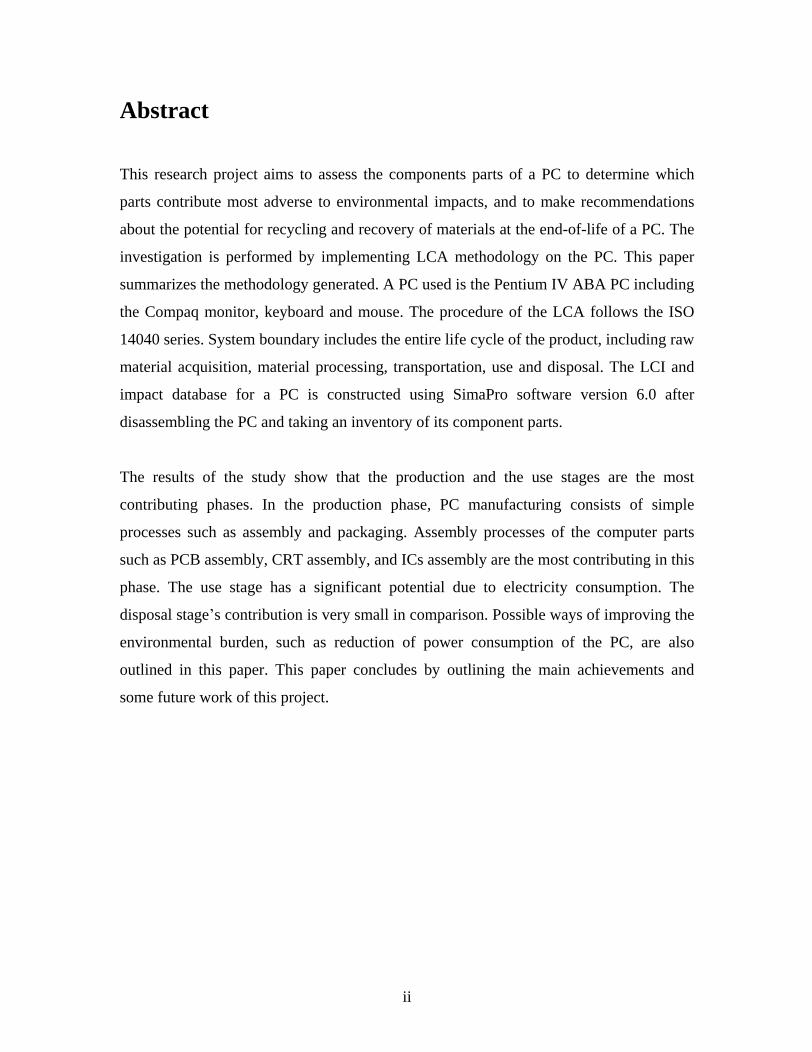
The desktop cabinet is made from metal frame, hard disk socket, a cover and a front.
Figure 5-1F shows the desktop cabinet disassembled.
There are two types of cables, assumed to be made, one from copper and PS and the other
made of PVC and copper.
Figure 5-1G: data cables and the mains cables from a PC system

30
Packaging for the control unit is a cardboard box and insert plus sponge. Since William et
al. (2003) show that ICs are significant, I treated them separately from the PCB. All the
ICs weights were taken together for each PC element.
Table 5-1A: Parts and Materials in the Control Unit
Parts Weight (g) Material
Motherboard
Printed circuit board with
components
930 Polyester/Al/PVC/Steel/Phenol/Epoxy/
Cu/Pb/Ceramic/PP/ Si2O3
Cooling body for processor 40 Aluminum
SUM 970
1.44MB, 3.5 floppy drive
Casing 340.2 Aluminum sheet
Mechanical part 234.42 Steel
Rotating wheel 57.34 Assumption: alloy aluminum with
coating
Front cover 7.98 Aluminum
Printed circuit board with
components
31.14 Polyester/Al/PVC/Steel/Phenol/Epoxy/
Cu/Pb/Ceramic/PP/ Si2O3
SUM 671.08
Hard disk drive
Printed circuit board with
components
31.39 Polyester/Al/PVC/Steel/Phenol/Epoxy/
Cu/Pb/Ceramic/ Si2O3
Hard disk plates 101.21 Assumption: alloy aluminum with
coating
Casing 307.92 Aluminum
SUM 440.52
Disk drive/CDROM
Mechanical part 286.56 Steel
PCB with components 144.91 Polyester/Al/PVC/Steel/Phenol/Epoxy/

31
Cu/Pb/Ceramic/PP/ Si2O3
Casing 433.43 Aluminum
Front cover (plastic) 18.83 ABS
SUM 883.73
ASTEC Power supply
Electrolytic capacitors 53.16 Al/Cu/Phenolic resin paper/PS
Inductor coils 64.78 PVC/insulated Cu+ Ferrite
Transformers 121.78 PVC/insulated Cu+ Ferrite
Cabinet 560.51 Steel
Cooling body 80.77 Aluminum
Heat sink 54.49 Aluminum
PCB with components 79.47 Polyester/Al/PVC/Steel/Phenol/Epoxy/
Cu/Pb/Ceramic/PP/ Si2O3
Cable and plug 115.96 Cu/PVC/PS
SUM 1130.92
Desktop cabinet
Metal frame 2735.65 Electroplated steel
Hard disk socket 263.26 Steel, electroplated
Cover 2200 Steel
Front 272.19 ABS
SUM 5471.1
Cables
Flat band cable 181.37 Cu/PS
Mains cable 181.14 Cu/PVC
SUM 362.51
Packaging for Control Unit
Box 1800 Cardboard
Insert 414.5 Cardboard
Packaging Material 175 EPS/Sponge
SUM 2389.5

32
ICs 38.91
TOTAL 12358.27
Table 5-1B shows the different parts and weights of the monitor. These are a cabinet that
is made of flame retarded ABS, foot and socket, CRT with electronic gun, cables and
printed circuits boards with components, electrolytic capacitors, choking coils and
transformers. Materials used in the parts of the PC monitor were obtained from a report
by Kim et al. (2000) and from own personal comparison, assumptions and knowledge. A
table from Huisman et al. (2004, p.14) on the product composition of 17-inch CRT
monitor is included in Appendix C which confirms the data that I used at least in part.
Figure 5-2A: shows the printed circuit board with components and some of the
electrolytic capacitors, transformers, choking coils being pulled off the board
The CRT consists of panel and funnel glass, shadow mask, frame, inner shield, mount,
deflection yoke and a shrinking band for protection. The electronic gun consists of steel,

33
glass pillar, hollow nickel tubes and tungsten wire. Figure 5-2B shows these internal
components of a CRT monitor.
CRT glass material is a very special type with a lot of lead in it. There is approximately
2-3 kg of insoluble lead encapsulated in the glass matrix of the funnel and faceplate in
each CRT (representing approximately 27% of content of the glass screen). There is an
additional 15-100 gm of lead present as soluble lead oxide in the frit , which is a type of
glass solder used to join the faceplate and funnel sections of CRTs (Computer and
Peripherals Material Project 2001).
The database for SimaPro does not have adequate data on lead glass. Due to lack of data
for this type of glass for the CRT monitor life cycle, the impact potentials that have been
calculated do not bear the exact load, but probably a small fraction of the total
contribution from the life cycle of this monitor.
Figure 5-2B: Internal components of a CRT monitor
(Source: http://www.deh.gov.au/settlements/publications/waste/electricals/computer-
report/production.html)
34
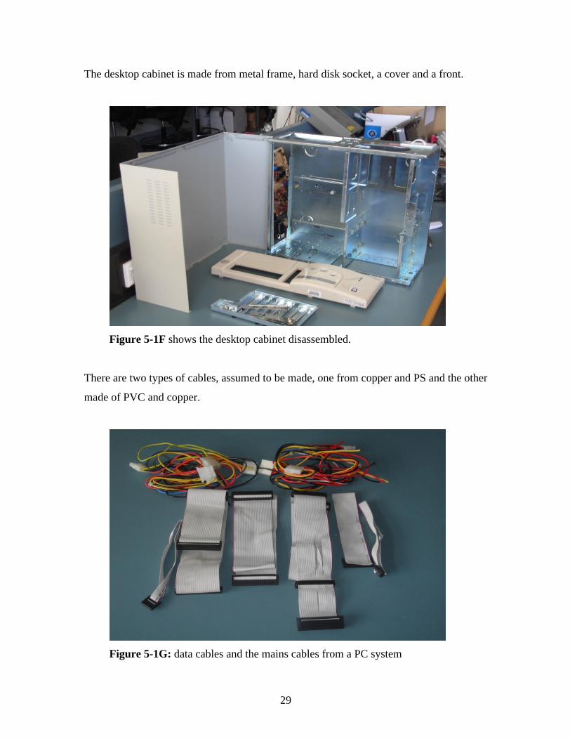
The packaging of the monitor is made of the cardboard box with a foam insert.
Table 5-1B: Parts and weights in the monitor Parts Weight (g) Material Monitor cable 290.4 Cu/PVC Foot/socket 338.37 ABS PCB casing 105.21 Brass/Steel PCB with components 107.15 Al/Steel/PP/Cu/Polyester/
Ceramic/Phenol/Epoxy/ Si2O3
Heat sink 280.96 Al Electrolytic capacitors 152.82 Al/Cu/Phenolic resin paper ICs 13.86 Al Inductor coils 93.81 PVC/Ferrite/Cu Transformers 509.39 Ferrite/Cu PCB with components 538.32 Al/Steel/PP/Cu/Polyester/
Ceramic/Phenol/Epoxy/ Si2O3
Cabinet 2480 ABS/PVC Frame 439 Steel CRT 7749 Glass/Steel/Cu/PVC/Paper SUM 13872.29 Packaging for the monitor Box 1780 Cardboard box Foam insert 535 EPS/Sponge/LDPE/HDPE SUM 2315 TOTAL 16187.29
Table 5-1C shows the different parts and weights of the keyboard. They are the cover, base and 102 keys, the base shielding and a cable with plugs and printed circuit board with components. The disassembly of the keyboard as shown on figure 5-3A, shows that it contains only a few components. On the PCB, there is one IC, two diodes, two resistors, three LEDs and one small electrolytic capacitor.
The packaging for the keyboard is a cardboard box with a plastic insert.

35
Figure 5-3A: shows the different parts of a keyboard
Table 5-1C: Parts and weights in the keyboard Parts Weight (g) Material PCB with components 14.22 Cu/Epoxy/Si2O3
Base shielding 59.58 Steel sheet Base 259.88 ABS Cover 143.53 ABS Keys 265.85 ABS Cable and plug 68.96 Cu/PVC SUM 812.02 Packaging for keyboard Box 310 Cardboard Plastic insert 35 Assumption: PS SUM 345 TOTAL 1157.02
Table 5-1D shows the parts and weights of the few components that are in the PC mouse. These are the 225mm2 PCB with only three components, the mouse ball, base, cover and the cable and plug. The packaging for the mouse is cardboard box.

36
Figure 5-4A: shows all the parts in the mouse
Table 5-1D: Parts and weights in the mouse Parts Weight (g) Material PCB with components 6.97 Cu/Epoxy/ Si2O3
Cover 24.95 ABS Base 25.32 ABS Mouse ball 31.25 Rubber Cable and plug 43.57 Cu/PVC SUM 132.06 Packaging for the mouse Cardboard box 45 Cardboard TOTAL 177.06
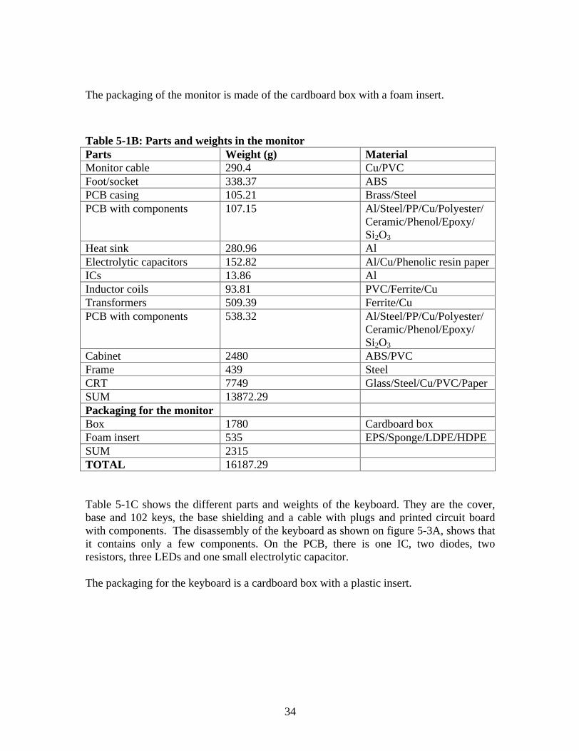
5.2 Calculation of the Environmental load of the PC
In order to calculate the environmental load of the PC, a model of the life cycle was
constructed as shown on figure 5-5A.
37
Figure 5-5A: shows the model of the life cycle of a PC from raw materials to disposal
5.2.1 Description of Life Cycle Stages
A primary concept of LCA is that life cycles are collections of stages. In theory, an
infinite number of stages might be defined. In practice, 4-6 stages usually are defined.
In this study the life cycle is defined as five stages: production of raw materials,
manufacturing, distribution, use and disposal. Transport will be considered within each
stage.
Glass 6.15kg
Plastic 3kg
Lead 816g
Copper 774.2g
PCB 509.5g
PCB 930g
ICs 13.86g
ICs 38.91g
Plastic 615.6g
Mould Plastic
Mould Glass
Assemble CRT monitor 15kg
Assemble Control Unit 12kg
PC Assembly 29kg
Transport to Twmba in 28-ton truck, 160km
Transport from W/sale to USQ, 7km
Transport to Brisbane in ship, 6000km
Disposal, 70% landfill & 30% recycle
Use 8hrs/day for 1200days
Mould Plastic
Steel/Al/Cu 7kg

38
5.2.1.1 Production of Raw Materials
The extraction and refining of raw materials like oil, natural gas, iron and other metals
are included here. So are extractions of raw materials for production of e.g. metal casing,
glass etc. The productions of some materials like glass, glass fibre, glass textile, copper
foil, and laminates for printed circuit boards are also included in the raw material stage.
5.2.1.2 Manufacturing
The manufacturing includes all processes for manufacturing the PC. These are metal
coating processes such as electroplating, injection molding of plastics; production of the
CRT (which includes the glass production but excluding the extraction of the raw
materials for the glass); production of the printed circuit board (from laminate) and
semiconductors, wave soldering etc.
5.2.1.3 Distribution
The PC is transported from a European/Asian PC manufacturer to the salesroom with a
truck larger than 16 tons. From the salesroom to the office it is transported by a van.
The driving distance for the truck is more kilometers as compared to van. For example,
the PC being studied here is transported from Malaysia to Brisbane by ship for a distance
of approx. 6000 km; and from Brisbane to Toowoomba at a distance of approx.160 km
by a 16-ton truck; and finally from a wholesale in Toowoomba to USQ office by a
delivery van. In each case the carrying capacity of transportation is calculated. For
instance, transporting this PC from Malaysia, the carrying capacity is 6000 km * 0.029
tonnes = 174 tonne*km.

39
5.2.1.4 Use
Power consumption for the monitor is 104.5 Watts and 39.13 Watts for control unit,
which includes power consumption of the keyboard. The base case PC has no energy
saving facilities and therefore consumes 143.63 Watts when turned on. The lifetime of
the PC is set to 5 years. This time span is the one companies use for writing off a PC in
their accounts. After 5 years in an office the first user of the PC is likely to get a new
computer. Then the PC is either thrown out or passed on to another user in the office or
given to an employee and used at home. Only the first life of the PC is considered in
this LCA. After 5 years, the PC is disposed. The PC is estimated to be turned on for 8
hours per day, 240 days per year (Byrre, T. 2005, pers.comm. 15 July). Altogether it runs
for 9600 hours during its lifetime. Therefore the energy that is consumed is around
1.3788MWh during its use.
5.2.1.5 Disposal
Disposal routes of general household waste in Australia have been used to estimate PC
disposal routes (Computer & Peripheral Material Project). According to this scenario,
63% of the PCs are sent to landfills, 22% to incineration and 15% to recycling. The same
pattern is assumed for the packaging. PCs sent to landfills are assumed to be disposed of
in landfills for household waste (bulk waste). Emissions to waste water from the
leachates of metals within the first hundred years are taken into account. Emissions of
methane from decomposition of cardboard in landfills are included.
Representing an average recycling situation in the European Union countries the metals
and the PCB with components is assumed sent to secondary metal works where steel,
aluminum, copper, lead, zinc, and silver and gold are reclaimed. The recovery is 97% for
steel, 95% for aluminum and 100% for the other metals. Metals not mentioned above are
lost in the recovery process. The glass/silicon oxide from the PCB is landfilled as
hazardous waste.

40
All other parts of the computer are landfilled (LCA Study of the Product Group Personal
Computers in the EU Ecolabel Scheme 1998).
All the above data for all the stages was used in SimaPro to perform a life cycle
assessment of the PC.

41
CHAPTER 6
Life Cycle Impact Assessment
The impact assessment method used in this study is the Eco-indicator 99 method that has
already been discussed in chapter 3 (outlined in SimaPro software - methods). In this
method normalization and weighting are performed at damage category level. There are
three damage category levels, human health, ecosystem quality and resources. The units
that are used in human health are DALY (disability adjusted life years; which means
different disability caused by diseases are weighted); in ecosystem quality PDF*m2yr is
used as the unit where PDF means potentially disappeared fraction of plant species; and
finally MJ surplus are used in the resources. The impact categories and the
characterization factors in this method are; acidification/eutrophication, fossil fuels, land
use, ozone layer, radiation, minerals, climate change, respiratory in-organics, respiratory
organics, eco-toxicity and carcinogens.
Impact assessment may be broken down into two steps: classification and
characterization. Classification in SimaPro V6.0 is defined as the grouping of inputs and
outputs of the life cycle system, usually reported by weight, under categories of
environmental impact that these input/output engender. For instance, air emissions that
are believed to contribute to acid rains are classified under acidification, while those that
are believed to be greenhouse gases are classified under global warming. Fossil fuels on
the other hand are classified under the abiotic resources. It is also possible to assign
emissions to more than one impact category at the same time; for example SO2 may also
be assigned to an impact category like Human health, or Respiratory diseases.
With characterization, inputs/outputs are aggregated in a category into a single indicator
that is meant to reflect the sum environmental burden for that category. Aggregation is
done on the basis of common units that are agreed to represent an equivalent impact to

42
the environment; these are known as equivalence factors. These factors should reflect the
relative contribution of an LCI result to the impact category indicator result. For example,
on a time scale of 100 years the contribution of 1 kg CH4 to global warming is 42 times
as high as the emission of 1 kg CO2. This means that if characterization factor of CO2 is
1, the characterization factor of CH4 is 42. Thus, the impact category indicator result for
global warming can be calculated by multiplying the LCI result with the characterization
factor. Table 6-1A and 6-1B show the classification of emissions to air and the possible
categories to be included in characterization, respectively.
Table 6-1A: Classifications of emissions to Air
Substance Global
warming
Respiratory effects
(in-organics)
Acidification/
Eutrophication
Ecotoxicity Ozone layer
depletion
Ammonia + +
Arsenic +
Benzene +
Benzo(a)pyrene +
Butane +
Cadmium +
Carbon dioxide +
Carbon monoxide + +
Chloroform + +
Chromium +
Chromium VI +
Dinitrogen monoxide +
Dioxins +
Ethane + +
Fluoranthene +
Heavy metals,
unspecified
+
Lead +
Mercury +
Metals, unspecified +
Methane + +
Nickel +
Nitric oxide +
Nitrogen dioxide +
Nitrogen oxides + +
Polycyclic aromatic
hydrocarbons (PAH)
+

43
Particulates +
Phenol +
Sulphur hexafluoride +
Sulphur dioxide + +
Sulphur oxides + +
Toluene +
Zinc +
+ means contribution to that category
Table 6-1B: Environmental Impact Categories
Classification Category Examples of
species included
Equivalence factor
for
characterization
Comment
Abiotic resources Fossil fuels and
minerals
Weight ( MJ per kg
extraction)
Fuels are split into
renewable and
non-renewable
resources
Climate change (Global
warming)
CO2, CO, CH4 100-year GWP as
defined by IPCC,
with CO2 as the
reference
Ozone layer depletion CFCs, Halons,
HCFCs and other
chloro/bromo
compounds
ODP as defined by
the WMO, with
CFC-11 as the
reference.
Eco-toxicity Heavy metals m3 air, water or soil The amount of air,
water or soil
needed for
dilution to no
effect level
Acidification/Eutrophication SO2, NOx, NO3-,
NO2
Acid and nitrogen
contents with SO2
and NO3- as
references

44
Respiratory effects In-organic
compounds
(Source: Atlantic Consulting and IPU, LCA Study of the Product Group Personal
Computers in the EU Ecolabel Scheme)
The current state of life cycle inventory analysis and the available databases (in SimaPro)
is such that while consumption of energy and resources is well covered, data are still very
incomplete for the emissions of most environmentally hazardous substances such as lead
which is used in CRT glass. Due to lack of data for these types of emissions from the
large majority of processes of the life cycle, the impact potentials for some of the impact
categories end up not representing the total contribution from the life cycle to these
impact categories. As a result of this, the results obtained from this study will be
compared to the other products of the same and to other methods that has been used on
the same products.
6.1 Validation of the Eco-indicator 99 Methodology
In comparison of the Eco-indicator methodology with other methods that can be used for
the assessment, Luo et al. (2001) have analyzed laptops, office telephones and alternative
part designs using four different methods. These are Eco-indicator 95, Eco-indicator 99,
Ecological Footprint and Eco Pro. In each case the results are broadly similar from each
method and all agree about which of the two alternative products are environmentally
better.
This evidence suggests that the Eco-indicator 99 is as valid as the other methods in
deriving measures of environmental damage to any product. Hence the results obtained
from this methodology will be as sound as the others.

45
6.2 Results and Discussions from the Inventory Analysis
There are so many environmental parameters that are included in the life cycle analysis.
A few of those are selected here for discussion. Figures 6-1A and 6-1B show the
consumption of resources in terms of fossil fuels and minerals. Contribution ratio of each
environmental burden as a percentage is also shown on the figures.
0
20
40
60
80
100
120
140
160
180
200
1 2 3 4 5 6 7 8 9 10 11
Aluminum, in ground (1%) Lead, in ground (5%)
Copper, in ground (94%)
Environmental burden
MJ surplus
Figure 6-1A: Consumption of resources in life cycle of a PC (minerals).
The use of copper in ground is approx. 187 MJ surpluses which is 94% of the total
consumption of minerals for the PC life cycle. Lead contributes 5% of total load.

46
0
200
400
600
800
1000
1200
Coal, in ground Natural gas Oil, crude
MJ surplus
72%
15%13%
Figure 6-1B: Consumption of fossil fuel resources in the life cycle of a PC
The energy-related resources like coal, natural gas and crude oil are shown in figure 6-1B
with their contributions to the total load on the consumption of fossil fuels on the PC life
cycle. Coal which is used for generating electricity is consumed at a ratio of 72%, while
crude oil is used at a rate of 13% of the total fossil fuels consumption.

47
0
0.0001
0.0002
0.0003
0.0004
0.0005
0.0006
0.0007
0.0008
CO2 NO Particulates SO2 SO Others
16%
29%
6%
24%
19%
5%
DALY
Figure 6-1C: Environmental emissions in the life cycle of a PC
Figure 6-1C shows a contribution of 16% of carbon dioxide emissions on the
environment throughout the life cycle of the PC. These emissions are harmful to human
health. Nitrogen oxides NOx are the ones with the largest emissions (29%) followed by
sulfur dioxide (SO2) with 24% of total emissions to the environment.
6.3 Results and Discussions from Impact Assessment
The results of the classified and characterized inventory of the whole PC are presented
and discussed here. This section is divided into sub-sections in which the results of the
whole PC and all its peripherals (control unit, monitor, keyboard and mouse) will each be
discussed.

48
6.3.1 The Whole PC
Figure 6-2A shows the whole characterized results of the environmental impact of a PC
including packaging on a single score. A single score is where the data of the inventory
table is transformed into damage scores which can be aggregated. All the category
impacts of the impact assessment method used are represented. The characterized data
shows that use of resources caused by depletion of fossil fuels have the largest
contributions of about 45%, followed by the respiratory in-organics with 32%, climate
change having 7.5% and minerals with a contribution of about 6% on the environmental
performance of the PC.
Since there are many impact categories associated with this assessment method, some of
them, mostly those that contribute more to the total environmental impact of the PC are
selected and presented. Tabulated results for all of the impact categories are presented in
Appendix B.
Figure 6-2A: Characterization results of the environmental impact of whole PC system

49
In figure 6-2B and similar networks they follow, the top yellow box is a product stage
called the PC life cycle. The life cycle can link up to:
One assembly (which may have subassemblies). For instance, the sub-assemblies of
the PC assembly (blue box) are the control unit, CRT monitor, keyboard and
mouse.
One or more use process (grey box), in this case electricity.
A waste or disposal scenario (red box).
Processes (such as printed circuit board assembling process) are linked to the product
stage by a flow of arrows (note the direction of the waste scenario process). The thickness
of the line represents the contribution to the environmental load from a process, sub-
assembly or assembly stage. The small bar chart in a block indicates contribution to an
indicator.

50
The characterized results for the use of fossil fuels in figure 6-2B shows that the largest
contributions of impact come from the use phase where they are caused by the electricity
consumption during use. This constitutes 61.3% of the total performance, while the
second most contributing factor is the PC assembly which includes the production and
the manufacture stages. These stages contribute 35.8% of the total contributions of the
use of fossil fuels. The disposal stage only contributes a small amount of less than 3%. In
the PC assembly process, the control unit contributes approximately 25% of the
environmental impacts, which mainly comes from the ICs and the printed boards; while
the CRT monitor contributes only about 10%. The keyboard and the mouse both have a
small impact contribution less than 1%.
Figure 6-2B: Characterized network shows aspects of PC life cycle and relative use of
fossil fuels

51
The impact category climate change which is also known as global warming includes
effect of gases such as carbon dioxide, carbon monoxide, dinitrogen monoxide, ethane,
and methane and sulfur hexafluoride. Tabulated results are at Appendix B. The data
shows that carbon dioxide (CO2) is the most contributing environmental impact with
approximately 87%. Figure 6-2C shows that the electricity consumption in the use phase
contributes a fair amount to environmental burdens. A percentage of 63.7 are contributed
from this phase. CO2 emission in the air is as a result of more energy that is consumed in
the use phase. The PC assembly process only contributes approximately half of the
contribution by the use phase, with the ICs from the control unit contributing more than
any other material/parts.
Figure 6-2C: Characterized network showing the aspect of climate change (global
warming) as a result of the life cycle of a PC

52
The characterized network for the depletion of minerals shown on figure 6-2D, shows
that the PC assembly contributes significantly to the burden; the printed boards, copper
and lead being the main contributors on all of the PC elements. A table showing the
results of the substances that contribute to the characterized minerals category is in
Appendix A. The results show that the most contributing substance is copper with 93.5%,
lead 4.8% and aluminum with 1%. The control unit assembly shows to be contributing
more than the CRT monitor assembly with contributions coming from the printed boards
and copper.
Figure 6-2D: Characterized network shows aspects of PC life cycle and resource
consumption (use of mineral resources)

53
The respiratory in-organics category also shows that the use phase is the largest
contributor of burden. This contribution is caused by the amount of electricity that is
consumed during use. The consumption of energy amounts to more than 65% of the total
burden as can be seen from figure 6-2E. The PC assembly accounts to approximately
30%, with the control unit contributing almost twice the CRT monitor assembly. The
keyboard and the mouse again contribute a small amount of less than a percentage. The
parts that have the most contributing impacts are the printed boards which quadruple the
burdens from ICs. With the substances, nitrogen oxides (NOx) seemed to be having the
most common environmental impacts, with 37% being contributed. Sulfur dioxide (SO2)
was the next followed by sulfur oxides, with 31% and 24% contribution respectively.
Figure 6-2E: Network shows aspects of PC life cycle and relative contributions to
respiratory in-organics

54
Another category that the PC system has environmental impacts on is acidification and
eutrophication. Examples of species in these categories are nitrogen oxides (NOx), sulfur
dioxide (SO2) and nitric oxide (NO3). The results of which are tabulated in Appendix B
show that nitrogen oxides are the most environmental impact contributors with
approximately 70%, followed by sulfur dioxide with approx. 17 %. Sulfur oxides
contribute 13% of the total load in acidification/eutrophication. Electricity consumption
in the use phase is the largest contributor, with 69.8% contribution, while the PC
assembly which includes production and manufacture stages contributes 26.7%; and the
disposal (waste) stage has 3.5% contribution. Figure 6-2F shows that the assembly of the
control unit (16.7%) is the next contributor after electricity consumption, and the CRT
monitor assembly accounts for less than 9%. The printed board is the dominating
contributor in all the elements of the PC, followed by the ICs. The ICs contribute almost
one half of the printed board contribution.
Figure 6-2F: Characterization network of acidification/eutrophication

55
Eco-toxicity includes species such as heavy metals. In this category copper that is used in
the production and manufacture of the PC assembly is the most environmental
contributor with more than 70% of total contribution of the PC; nickel 13%; and lead 7%.
The PC assembly in this category contributes more environmental burden than the use
phase. The contribution is illustrated in figure 6-2G where the PC assembly accounts for
90%, while the use accounts for 10%. The control unit is the most contributor with
55.9%; most of the impact coming from the printed board. The control unit is the next
contributing element with 32.6%; again most of the impact coming from the printed
board (27.9%) and the glass (4.41%) because lead is used as a raw material in the glass
tube. Energy consumption during the PC assembly contributes approx. 10%. Once again
the keyboard and the mouse have little impact.
Figure 6-2G: Characterization network on the results on eco-toxicity in the life cycle of a
PC

56
The assessment shows that of the impact categories discussed, electricity consumption
during use is the main issue to most of the category impacts that are caused by the PC,
except of course for eco-toxicity and minerals where the PC assembly is the most
contributing factor. As such the use phase is seen as the most contributing phase to
environmental performance of the PC. The printed board assembly on the other hand is
one of the most contributing components in the PC assembly on all the category impacts.
6.3.1.1 Normalization
Normalization is a procedure needed to show to what extent an impact category has a
significant contribution to the overall environmental problem (Goedkoop & Oele 2004).
This is done by dividing the impact category indicators by a Normal value. There are
different ways to determine the Normal value. The most common procedure that is
used in SimaPro is to determine the impact category indicators for a region during a year,
and if desired, divide the result by the number of inhabitants in that area.
Normalization serves two purposes:
1. Impact categories that contribute only a very small amount compared to other
impact categories can be left out of consideration, thus reducing the number of
issues that need to be evaluated.
2. The normalized results show the order of magnitude of the environmental
problems generated by the products life cycle, compared to the total
environmental loads in a specific region.
The three damage categories and the eleven impact categories in Eco-indictor 99 have
different units. In order to use a set of dimensionless weighting factors, these categories
are made dimensionless. Hence the normalized data/results for the PC were also taken.
Figure 6-2H shows the normalized results of the impact categories. The contributions to

57
fossil fuels from a PC are almost 57% of the total contributions of impact categories.
Contribution to climate change accounts to approx. 7% of the total contributions.
Figure 6-2H: Normalization of environmental impact potentials of the whole PC
6.3.1.2Damage assessment
The final step of assessment in Eco-indicator 99 method is the damage assessment, as has
already been mentioned in chapter 3 (Project Methodology). In this step the impact
category indicator results that are calculated in the characterization step are added to form
the damage categories. Impact categories are grouped according to the same damage type
they have (like human health have the same unit DALY).
Figure 6-2I shows that the damage to resources is the most contributing in the
environmental performance of the PC. Depletion of resources contributes approx. 51%
done by the PC; human health comes next with 40% and ecosystem quality with 9%.
Resources depletion includes the electricity/energy consumption during extraction of
materials, production and manufacture, and the use of the PC.

58
Figure 6-2I: Damage assessment of the life cycle of a PC on a single score
The damage categories are also normalized as can be seen on figure 6-2J. The damage
categories are normalized on a European load (damage divided by population per year).
Normalized results on resources show a contribution of 29% of one person s contribution
(0.29 MJ energy surpluses) per year. The contribution to human health from one person is
15% per year, while 2% contribution per year from one person is caused on ecosystem
quality.
Figure 6-2J: Normalized damage category results

59
Figure 6-2K shows that the damage to resources accounts to 51% of the total damage by
the PC whole life cycle. Damage to human health is 40% and to ecosystem quality is 9%
on a weighted scale of the whole life cycle.
Figure 6-2K: Damage assessment results of the PC life cycle on a weighted scale
6.3.2 Control Unit
Figure 6-3A shows the characterized emissions for the control unit including packaging.
Results are given for all the lifecycle stages on a single score. Some of the impact
categories are also represented in figures 6-3B to 6-3E. The normalized data for the
environmental impacts is shown on figure 6-3F. The normalized damage categories
results are shown on figure 6-3G, followed by the weighted damage assessment results on
figure 6-3H. The damage assessment figure on a single score for the control unit is shown
on figure 6-3I.

60
Figure 6-3A: shows the characterized results of the environmental impacts for the
control unit
The figure shows that the use of fossil resources has the largest environmental load,
followed by respiratory effects (in-organics), and the global warming potential (climate
change) and mineral resources.

61
Figure 6-3B: shows the characterized effects of global warming due to climate change
caused by the control unit
The results show that the effect on global warming potential due to climate change for the
control unit was largest in the production stage, and second largest in the use stage. The
effects in the disposal stage are very small (less than 1%).

62
Figure 6-3C: shows the aspects of the control unit life cycle and the relative use of fossil
fuels (resources)
Depletion of fossil resources is largest in the production phase followed by the use phase
with a contribution of approx. 40%. The largest contribution on the control unit came
from the ICs with approx. 32% and then the printed circuit board with about 24%. The
disposal stage once again poses little effect.

63
Figure 6-3D: Characterized results of mineral resources potential due to the control unit
life cycle
Figure 6-3D shows that almost all of the environmental impact was produced in the
production stage. In this stage the largest index on the use of mineral resources was in the

64
printed circuit boards of the control unit. This is because of the energy used in extracting
the mineral metals used to assemble the PCB. The second largest contribution is from
copper with approx. 22%.
Figure 6-3E: Characterization results of acidification/eutrophication index in the life
cycle for the control unit.

65
Environmental impact in figure 6-3E is largest in the use and production stages in
acidification/eutrophication analysis for the control unit, with the largest contribution
coming form the printed circuit boards, then the ICs.
Figure 6-3F: Normalized environmental potentials for control unit with packaging
Figure 6-3F shows that the consumption of resources (that is, fossil fuels and minerals)
by one person s relative share per year is approx. 13%, while effects of climate change
contribute only 1% to one person per year.

66
Figure 6-3G: shows the normalized damage categories of the control unit with packaging
Figure 6-3G shows that the contribution of damage to human health from one person is
6% per year; on ecosystem quality is 1%; and on damage to resources is 12% of one
person per year.

67
Figure 6-3H: shows the weighted damage assessment results for the control unit life
cycle
The results on a weighted scale show that the damage to ecosystem quality is approx. 9%,
and to human health is 38% of the total contribution from the life cycle of the control
unit. Similar results are shown on a single score on figure 6-3I.

68
Figure 6-3I: Damage assessment for the control unit on a single score
6.3.3 CRT Monitor
Figure 6-4A shows the characterized results of the environmental load of a CRT monitor
life cycle with packaging on a single score. Like the control unit, only a few of the impact
categories are presented. As previously pointed out in chapter 5, the results of the CRT
monitor do not represent the total contribution as assumptions for glass in the CRT were
made. The lead glass of which the CRT glass consists is not available in SimaPro
database. These are presented on figures 6-4B to 6-4E. The normalized environmental
impact potential is represented on figure 6-4F. The damage category figures for the CRT
monitor are presented on figures 6-4G to 6-4H.

69
Figure 6-4A: the characterized environmental impact potentials of the CRT monitor
The figure shows that the use of resources (fossil fuels and minerals) has the largest
environmental load, followed by respiratory effects (in-organics), and the global warming
potential due to climate change.

70
Figure 6-4B: Characterized results shows aspects of the CRT monitor life cycle and
effect on climate change (global warming potential)
The results show that most of the global warming potential comes from the use stage
followed by the production stage. The printed circuit board and the ICs are the most
contributing parts in the life cycle of the CRT monitor in this case.

71
Figure 6-4C: Characterized results of acidification/eutrophication index for the monitor
The results obtained for acidification/eutrophication analysis show that the environmental
impact is large in the use and production stages, with the printed circuit board having the
largest load in the production stage.

72
Figure 6-4D: shows the aspects of the life cycle for the CRT monitor and relative
use of fossil fuels (resource consumption index of fossil fuels)
Figure 6-4D shows that the use of fossil resources is largest in the use stage of the life
cycle of a monitor.

73
Figure 6-4E: shows characterized minerals resources index for the life cycle of
the CRT monitor
The above figure shows that almost the entire load on mineral extraction is produced in
the production stage. The largest index was on the printed circuit board, followed by
copper and lead.

74
Figure 6-4F: Normalized damage assessment for CRT monitor life cycle
A 16% contribution of one person per year to damage to resources is observed in the
normalized results of the monitor life cycle. The relative share of damages to human
health is 9% per person per year.

75
Figure 6-4G shows the weighted results of the damage categories of the life cycle of the
CRT monitor. Damage to human health is approx. 43% of the total environmental load of
the life cycle of the CRT monitor. The damage to ecosystem quality amounts to 9% of
the total load. The same results are presented on a single score on figure 6-4H.
Figure 6-4G: Weighting of the damage categories for the CRT monitor life cycle

76
Figure 6-4H: Damage assessment of the life cycle for the CRT monitor on a single score
Results on a single score same as in figure 6-4G.
6.3.4 Relative Contributions of the PC Elements
The following tables show the relative contributions of the elements of the PC to the
environmental impact potential and the damage potential. Detailed tables for the whole
PC contributions and each element s contributions to both environmental impact potential
and categorized damage potential are on Appendix B.
Table 6-1C: Contributions to Environmental Impact Potential, PC by Element
Environmental impact
categories
Control
Unit
CRT
Monitor
Keyboard &
Mouse
Total
Fossil fuels 41.5% 56% 2.5% 100%
Minerals 53.5% 44% 2.5% 100%
Ozone layer 44% 47% 9% 100%
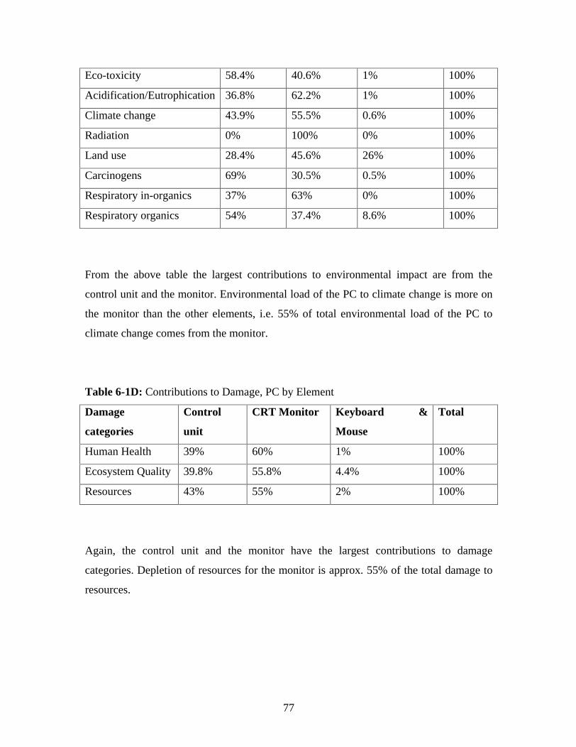
77
Eco-toxicity 58.4% 40.6% 1% 100%
Acidification/Eutrophication
36.8% 62.2% 1% 100%
Climate change 43.9% 55.5% 0.6% 100%
Radiation 0% 100% 0% 100%
Land use 28.4% 45.6% 26% 100%
Carcinogens 69% 30.5% 0.5% 100%
Respiratory in-organics 37% 63% 0% 100%
Respiratory organics 54% 37.4% 8.6% 100%
From the above table the largest contributions to environmental impact are from the
control unit and the monitor. Environmental load of the PC to climate change is more on
the monitor than the other elements, i.e. 55% of total environmental load of the PC to
climate change comes from the monitor.
Table 6-1D: Contributions to Damage, PC by Element
Damage
categories
Control
unit
CRT Monitor Keyboard &
Mouse
Total
Human Health 39% 60% 1% 100%
Ecosystem Quality 39.8% 55.8% 4.4% 100%
Resources 43% 55% 2% 100%
Again, the control unit and the monitor have the largest contributions to damage
categories. Depletion of resources for the monitor is approx. 55% of the total damage to
resources.

78
6.4 Discussion of Overall Results
The results obtained from the analysis of climate change, acidification/eutrophication, use
of minerals and fossil fuels, eco-toxicity, ozone layer depletion and respiratory inorganics
show that the environmental impact on the PC was large in the use and production stages.
This means that if we would like to improve the environmental impact, then focus should
be on these stages of the PC life cycle. The disposal stage in all cases has very little effect
to the environmental impact. As already seen on the figures on the results, the
environmental impact in the use stage was generated as a result of electricity
consumption during use. The electricity consumption in the use stage for almost all the
environmental impact categories, show a much higher percentage on electricity
consumption than on the production processes of the PC life cycle. In the production
phases the most environmental impact potential came from the control unit and the
cathode ray tube monitor. The impact potentials are due to various causes. These causes
include among others the printed circuit board, ICs, steel, copper, lead, cathode ray tube
assembly etc. The loads in the keyboard and mouse are relatively small.
The cathode ray tube monitor is the heaviest assembly in the PC monitor having materials
such as glass, steel, copper, coating materials, etc. This makes the manufacturing process
of the cathode ray tube to be energy-intensive. The overall results for the cathode ray tube
monitor do not reflect to exact contribution to environmental load as assumption on the
glass was made since the data for the lead glass that is used in the CRT monitor was not
available in the SimaPro database.
The environmental potential for the printed circuit board production and ICs is assumed
to be mainly produced in the assembling process. Also the PCB has a large number of
parts mounted onto it which are assumed to be also contributing to the environmental
load. Kim et al. (2000, p.6) has the following to say about the printed circuit board
assembly process:

79
In the assembly process where the electronic devices are inserted onto the phenol resin
board, some of the electronic devices are arranged and attached to a paper roll and cut
automatically to the proper size for an inserting machine. Therefore, the inserting process
generates a large amount of paper and steel wire waste. After inserting electronic devices,
the board moves to the soldering process, followed by the cleaning process where steam
is used as a cleaning agent. The printed circuit board assembly is also energy intensive.
Metal cabinet (steel) which is used in the housing of most of the components such as the
hard disk drive (HDD), CD-ROM drive, and for the control unit itself, seems to have a
large contribution to the environmental impact than the plastic material casing.
It is therefore recommended that to reduce (improve) the environmental impact potential
of the PC, the following points should be considered:
Reduction of power consumption of the PC (this includes the monitor and control
unit) in the use stage. The energy consumption of the CRT monitor holds a strong
improvement potential as compared to the control unit, as it consumes almost
twice the energy consumed by the control unit. Needless to say, the energy
consumption of the control unit is also significant.
The printed circuit board assembling process and the ICs should be improved.
This can be achieved by reducing the number of parts on the board and
miniaturizing the boards.
Use of low power consuming displays such as LCDs.
Recovery of materials and re-use: this extends the use-life of the PC as the
motherboard, hard disk, etc may be upgraded. After upgrading the PC may be
used for another 3-5 years. A PC may also be bought at point of disposal and
again be used for another 3-5 years.

80
CHAPTER 7
Conclusions
7.1 Main Achievements of Objectives
This project was conducted with the aim of assessing the environmental impact of the life
cycle of a PC. This PC was manufactured in 1997 in Asia, and has been used for almost 5
years before being put in storage, awaiting disposal. The parts that contribute more to the
environmental load and possible ways of environmental improvements were to be
identified. This study shows that the use and production phases are the most contributing
stages in the life cycle. Of these two stages, the use stage was the most contributing to the
environmental impact than the production stage. The use stage shows that the impact was
generated as a result of electricity consumption during use; and in the production stage
the control unit and the CRT monitor assembly processes are the most contributors. The
parts contributing most from the control unit and the monitor are the printed circuit
board, ICs, cabinet housing that is made of steel, copper, and the cathode ray tube
assembly.
It is therefore based on the results of this study that the possible ways of reducing the
environmental burden of the life cycle of the PC are:
1. Reduce PC energy consumption the monitor as observed from the power
consumption measurements taken, consumes more power than the control unit. It
is also understood that even in stand-by mode, electronic devices consume power.
As a result the energy consumption of the monitor holds very strong improvement
potential than that of the control unit.

81
2. Improving the PCB and ICs assembling processes
many different materials of
which are of environmental concern are used in the construction of the PCBs such
as cadmium and lead. Flame retardants including organic halogenated or
brominated compounds and inorganic compounds (e.g. antimony compounds) are
used in the epoxy of resin of PCBs to prevent fires (Computer & Peripherals
Material Project 2001). Of course the brominated flame retardants are of
principal concern with regard to environmental and health risks. This is the area
that needs attention (getting rid of the brominated flame retardants or replacement
with non-toxic or problematic materials).
3. Extending the lifetime by allowing for the exchange of motherboard and the
upgrading of the memories.
4. Use of plastic materials in the housing of components.
5. Using low power consuming displays such as LCDs. LCDs are understood to be
consuming less power than the CRT monitor because of the fact that they have a
smaller amount of materials and a smaller number of components than the CRT
monitor.
The software (SimaPro 6) used in this study is user-friendly and a very powerful tool in
assessing the environmental impacts of products. With this software only the foreground
data (such as data for semiconductor devices, cathode ray tube resistors capacitors, etc.)
has to be collected; most of the background data such as glass, electricity, aluminum,
energy, materials production, packaging materials etc. are already available in the
software. The software is valuable as it uses diagrams to illustrate the flows, stages and
processes of life cycle of product. The use of scores, with reliable data sets and impact
categories in the software enables effective comparisons to be made between products
and processes. Of course any software has its on merits and de-merits. Most data on some
of the materials is not available on the database; limited data, questionable data quality

82
and varying regional relevancy (data is based on European data) is also a constricting
factor, as such the lack of confidence in data in these areas means the environmental
scores could be unreliable.
The impact assessment method (Eco-indicator 99) used is as valid as any other method in
SimaPro. A comparison of these methods by Luo et al. confirms this. Aggregation of
impact categories into damage categories (human heath, ecosystem quality and resources)
makes the analysis of the results more easily using this method than the other methods.
7.2 Further Work
There are some uncertainties with regard to the software package, because of the
imprecision of available data. As such sensitivities can be identified and varied to check
whether the results will have any change. Therefore suggestions in future are that the
assumptions that were made (such as weight of some of the PC components and its life
time), be changed; materials data for some parts such as the glass that was assumed to be
used in the CRT be improved to see whether these will have any effect on the conclusions
made from the analysis. It is also suggested that other impact assessment methods be
applied to verify the validity of the results obtained with Eco-indicator 99.

83
8.0 List of References
Atlantic Consulting and IPU 1998, LCA Study of the Product Group Personal Computers
in the EU Ecolabel Scheme, European Commission, Brussels.
Goedkoop, M & Spriensma, R 2001, The Eco-indicator 99: A Damage Oriented Method
for Life Cycle Impact Assessment; Methodology Report, 3rd edn, PR Consultants, the
Netherlands.
Goedkoop, M & Oele, M 2003, Introduction to LCA with SimaPro 6, PR Consultants
B.V., Armersfoot.
Guinee, JB 2002, Handbook of Life Cycle Assessment: Operation Guide to ISO
Standards [Online], Kluwer Academic Publishers, Dordrecht, Boston, Available:
http://site.ebrary.com.ezproxy.usq.edu.au/lib/unisouthernqld/Doc?id=10067324
[Accessed 10 May 2005].
Huisma, J, Stevels, ALN & Stobbe, I 2004, Eco-Efficiency Considerations on the End-
of-Life of Consumer Electronic Products , IEEE Transactions on Electronics Packaging
Manufacturing, vol. 27, no. 1, pp. 9-25.
International Organization for Standardization, 1997, Environmental management Life
cycle assessment: Goal and scope definition and inventory analysis, ISO, Geneva.
Kim, S, Hwang, T & Overcash, M 2000, Life Cycle Assessment Study of Color Computer
Monitor [Online], Available:
http://www.samsung.com/AboutSAMSUNG/SocialCommitment/EHSReport/Greenmana
gementreport/downloads/treatise7.pdf., [Assessed 6 June 2005].

84
Luo, Y, Wirojanagud, P & Caudill, RJ 2001, Comparison of Major Environmental
Performance Metrics and their Application to Typical Electronic Products , Proceedings
of the 2001 IEEE International Symposium on Electronics and the Environment, Denver,
USA, pp. 94-9.
Matthews, HS 2003, Information and Communications Technologies and
Sustainability , IEEE International Conference on Systems, Man and Cybernetics,
Pittsburgh, USA, pp.1760-5.
Norris, GA, Croce, FD & Jolliet O 2003, Energy Burdens of Conventional Wholesale
and Retail Portions of Product Life Cycles , Journal of Industrial Ecology, vol. 6, no. 2,
59-69.
Tekwawa, T, Miyamoto, S & Inaba, A 1997, Life Cycle Assessment; An Approach to
Environmentally Friendly PCs , Proceedings of the 1997 IEEE International Symposium
on Electronics and the Environment, San Francisco, USA, pp.125-30.
Udo de Haes et al. 2002, Life cycle impact assessment: Striving Towards Best Practice,
Society of Environmental Toxicology and Chemistry, Pensacola, FL.
United Nations Environment Programme, Industry and Environment, 1996, Life Cycle
Assessment: What it is and how to do it, UNEP, Paris.

85
9.0 Bibliography
Blazek, M, Carlson, J & DeBartolo, M 1998, Life Cycle Management of Personal
Computers in a Service Company , Proceedings of the 1998 IEEE International
Symposium on Electronics and the Environment, Oak brook, USA, pp. 275-79.
Erikson, EH 1994, The life cycle completed, Orton, New York.
Frey, SD, Harrison, DJ & Billet, EH 2000, Environmental Assessment of Electronic
Products using LCA and Ecological Footprint, Paper presented to Joint International
Congress and Exhibition, Berlin, Germany, 11-13 Sept.
Hancock, N 2005, Research Project: Project Reference Book, University of Southern
Queensland, Toowoomba.
International Organization for Standardization 1997, Environmental management: life
cycle assessment: life cycle impact assessment = Management environmental: analyze du
cycle de vie: evaluation de I mpact du cycle de vie, ISO, Geneva.
International Organization for Standardization 1996, Environmental management Life
cycle assessment: Part 1: Life cycle interpretation, ISO, Geneva.
Standards Association of Australia 1998, Life cycle assessment: principles and
framework, Homebush, NSW.
Smith, B & Summers, J (ed.) 1997, Communication Skills Handbook: How to succeed in
written and oral communication, 2nd edn, University of Southern Queensland,
Toowoomba.
86
Williams, ED, Ayres, RU & Heller, M 2002, The 1.7 Kilogram Microchip: Energy and
Material Use in the Production of Semiconductor Devices , Journal of Industrial
Ecology, vol. 36, no. 24, pp. 5504-10.
A dedicated search engine for LCA reports (n.d.) [Online], Available:
http://www.pre.nl/LCAsearch, [Assessed 12 May 2005].
Dead TVs (n.d.) [Online], Available: http://www.ecorecycle.vic.gov.au , [Assessed 20
March 2005].
Life Cycle Inventories
http://www.utexas.edu/research/ceer/che 302/ greenproduct/dfe/PDF/Lci.PDF
LCA of the Product Group Personal Computers in the EU Ecolabel Scheme (March
1998) [Online], Available:
http://europa.eu.int/comm/environment/ecolabel/pdf/personal_computers/lcastudy_pc_19
98.pdf , [Assessed 12 May 2005]
Electronic and Electronic Product Stewardship Strategy (n.d.) [Online], Available:
http://www.ephc.gov.au/ephc/product_stewardship.html/ , [Assessed 3 May 2005].
Electronics, Recycling and LCA [Online], Available:
http://www.nrc-recycle.org/resources/electronics/links.html, [Assessed 18 April 2005].
The electronic scrap (n.d.) [Online], Available:
http://www.deh.gov.au/industry/index.html , [Assessed 18 April 2005].
US Environmental Protection Agency Life Cycle Assessment (n.d.) [Online], Available:
http://www.epa.gov/dfe/pubs/comp-dic/lca , [Assessed 18 April 2005].

87
10 Appendix A
University of Southern Queensland FACULTY OF ENGINEERING AND SURVEYING
ENG 4111/2 Research Project PROJECT SPECIFICATION
FOR: Baipaki Pakson HIKWAMA
TOPIC: Life cycle assessment of a personal computer
SUPERVISOR: Mr. David Parsons
ENROLMENT: ENG 4111 S1, D, 2005; ENG 4112 S2, D, 2005
SPONSORSHIP: Faculty of Engineering and Surveying, USQ
PROJECT AIM: This project aims to assess the environmental impact of a PC by using LCA methods. Specifically, it aims to determine which parts contribute most to adverse environmental impacts, and to make recommendations about the potential for recycling and recovery of materials and any other action as a means of environmental improvement.
PROGRAMME: Issue A, 21st March 2005
1. Research background information of the current LCA technology and its associated standards.
2. Understand current methodology associated with the SimaPro software and its proper usage.
3. Disassemble a particular PC and construct an inventory of its component parts, and measure the energy use of a typical similar PC under a variety of conditions.
4. Construct a model of the life cycle of a particular PC from raw material to ultimate disposal.
5. Perform various analyses using SimaPro software. 6. Study relevant literature for comparison of results to similar products.
As time permits: 7. Design methods to achieve environmental gains with respect to computers. This
might include research on the current status of recycling technologies and markets.
AGREED:
(Student) (Supervisor) / /
/ /

88
11 Appendix B
LCI Input/Output Tables
The inventory input/output for the whole PC, control unit and CRT monitor are presented in this appendix. Section 11.1 presents the inventory results for the whole PC; section 11.2 presents the results for the control unit while section 11.2 presents inventory results for the CRT monitor.
11.1 The Whole PC
Table 11-1A: Damage Assessment to Ecosystem Quality in the PC system NO SUBSTANCE COMPARTMENT UNIT PC LIFE
CYCLE
Total PDF*m2yr 102 1 Occupation, arable Raw PDF*m2yr 2.09 2 Occupation,
construction site Raw PDF*m2yr 0.0169
3 Occupation, forest Raw PDF*m2yr -0.148 4 Occupation, industrial
area Raw PDF*m2yr 1.11
5 Occupation, industrial area, vegetation
Raw PDF*m2yr 0.445
6 Occupation, mineral extraction site
Raw PDF*m2yr 0.0093
7 Occupation, traffic area Raw PDF*m2yr 5.44 8 Occupation, urban,
continuously built Raw PDF*m2yr 0.214
9 Occupation, urban, green areas
Raw PDF*m2yr 3.03
10 Transformation, from forest,
Raw PDF*m2yr -0.207
11 Transformation, from mineral extraction site
Raw PDF*m2yr -0.00912
12 Transformation, from unknown
Raw PDF*m2yr -8.57
13 Transformation, to arable
Raw PDF*m2yr 6.54
14 Transformation, to industrial area
Raw PDF*m2yr 1.67
15 Transformation, to industrial area, vegetation
Raw PDF*m2yr 0.444
16 Transformation, to Raw PDF*m2yr 0.00912

89
mineral extraction site
17 Transformation, to shrub land, sclerophyllous
Raw PDF*m2yr 0.0012
18 Transformation, to urban, continuously built
Raw PDF*m2yr 3.2
19 Transformation, to water bodies, artificial
Raw PDF*m2yr 2.44
20 Ammonia Air PDF*m2yr 0.0678 21 Arsenic Air PDF*m2yr 0.0594 22 Benzene Air PDF*m2yr 3.4E-6 23 Benzene, hexachloro- Air PDF*m2yr 6.87E-13 24 Benzo(a)pyrene Air PDF*m2yr 0.000137 25 Cadmium Air PDF*m2yr 0.0934 26 Chromium Air PDF*m2yr 0.647 27 Chromium VI Air PDF*m2yr 0.153 28 Copper Air PDF*m2yr 0.253 29 Dioxins, Air PDF*m2yr 4.31E-5 30 Fluoranthene Air PDF*m2yr 7.5E-8 31 Heavy metals,
unspecified Air PDF*m2yr -2.3E-7
32 Lead Air PDF*m2yr 1.39 33 Mercury Air PDF*m2yr 0.0199 34 Metals, unspecified Air PDF*m2yr 0.106 35 Nickel Air PDF*m2yr 2.08 36 Nitric oxide Air PDF*m2yr 0.0142 37 Nitrogen dioxide Air PDF*m2yr 0.368 38 Nitrogen oxides Air PDF*m2yr 43.8 39 PAH, polycyclic
aromatic hydrocarbons Air PDF*m2yr 5.06E-8
40 Phenol, pentachloro- Air PDF*m2yr 1.01E-13 41 Sulfur dioxide Air PDF*m2yr 10.7 42 Sulfur oxides Air PDF*m2yr 8.54 43 Toluene Air PDF*m2yr 1.24E-6 44 Zinc Air PDF*m2yr 0.537 45 Arsenic, ion Water PDF*m2yr 0.00527 46 Benzene Water PDF*m2yr 2.95E-6 47 Benzo(a)pyrene Water PDF*m2yr -8.43E-9 48 Cadmium, ion Water PDF*m2yr 0.0592 49 Chromium Water PDF*m2yr 0.125 50 Chromium VI Water PDF*m2yr 3.44E-5 51 Chromium, ion Water PDF*m2yr 7.42E-6 52 Copper, ion Water PDF*m2yr 14.4 53 DNOC Water PDF*m2yr -1.65E-10

90
54 Fluoranthene Water PDF*m2yr -6.09E-9 55 Lead Water PDF*m2yr 0.134 56 Mercury Water PDF*m2yr 0.000129 57 Metallic ions,
unspecified Water PDF*m2yr 0.00346
58 Nickel, ion Water PDF*m2yr 0.444 59 PAH, polycyclic
aromatic hydrocarbons Water PDF*m2yr 1.73E-8
60 Phenol, pentachloro- Water PDF*m2yr -1.27E-8 61 Phthalate, dioctyl- Water PDF*m2yr 4.14E-13 62 Toluene Water PDF*m2yr 1.23E-5 63 Zinc, ion Water PDF*m2yr 0.0648 64 Arsenic Soil PDF*m2yr 0.000975 65 Cadmium Soil PDF*m2yr 0.00201 66 Chromium Soil PDF*m2yr 0.000336 67 Chromium VI Soil PDF*m2yr 0.000241 68 Copper Soil PDF*m2yr 0.00482 69 Lead Soil PDF*m2yr 5.21E-5 70 Mercury Soil PDF*m2yr 0.000101 71 Nickel Soil PDF*m2yr 0.106 72 Zinc Soil PDF*m2yr 0.0181
Table 11-1B: Damage Assessment to Human Resources for the PC system NO SUBSTANCE COMPARTMENT UNIT PC LIFE
CYCLE
Total DALY 0.00233 1 2-Propanol Air DALY 5.88E-10 2 Acetaldehyde Air DALY 7.5E-11 3 Acetic acid Air DALY 1.07E-10 4 Acetone Air DALY 6.88E-9 5 Acrolein Air DALY 4.62E-14 6 Acrylonitrile Air DALY 2.85E-9 7 Alcohols, unspecified Air DALY 1.05E-7 8 Aldehyde, unspecified Air DALY 6.17E-10 9 Arsenic Air DALY 2.47E-6
10 Benzaldehde Air DALY 1.3E-14 11 Benzene Air DALY 3.67E-9 12 Benzene, ethyl- Air DALY 5.55E-10 13 Benzene, hexachloro- Air DALY 1.46E-15 14 Benzene, pentachloro- Air DALY 9.91E-20 15 Benzo(a)pyrene Air DALY 3.84E-9 16 Butane Air DALY 3.93E-9 17 Butene Air DALY 3.38E-11
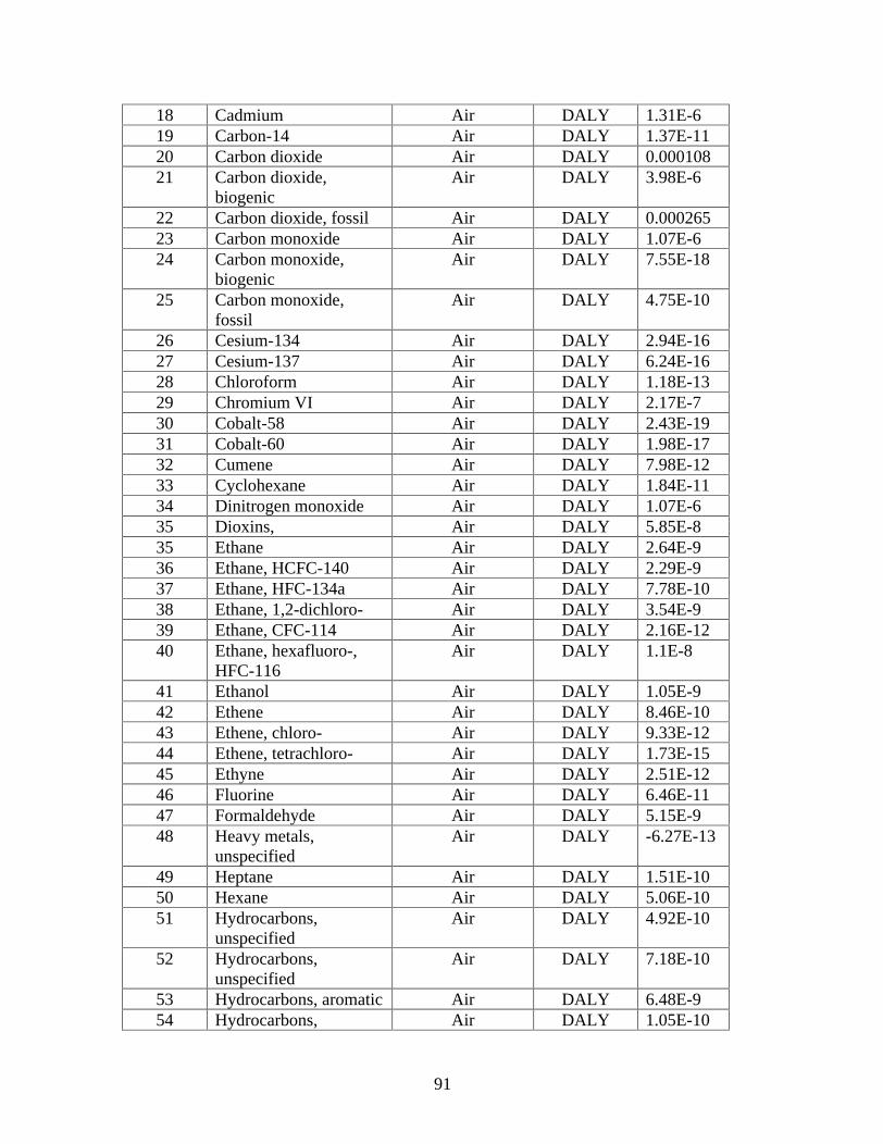
91
18 Cadmium Air DALY 1.31E-6 19 Carbon-14 Air DALY 1.37E-11 20 Carbon dioxide Air DALY 0.000108 21 Carbon dioxide,
biogenic Air DALY 3.98E-6
22 Carbon dioxide, fossil Air DALY 0.000265 23 Carbon monoxide Air DALY 1.07E-6 24 Carbon monoxide,
biogenic Air DALY 7.55E-18
25 Carbon monoxide, fossil
Air DALY 4.75E-10
26 Cesium-134 Air DALY 2.94E-16 27 Cesium-137 Air DALY 6.24E-16 28 Chloroform Air DALY 1.18E-13 29 Chromium VI Air DALY 2.17E-7 30 Cobalt-58 Air DALY 2.43E-19 31 Cobalt-60 Air DALY 1.98E-17 32 Cumene Air DALY 7.98E-12 33 Cyclohexane Air DALY 1.84E-11 34 Dinitrogen monoxide Air DALY 1.07E-6 35 Dioxins, Air DALY 5.85E-8 35 Ethane Air DALY 2.64E-9 36 Ethane, HCFC-140 Air DALY 2.29E-9 37 Ethane, HFC-134a Air DALY 7.78E-10 38 Ethane, 1,2-dichloro- Air DALY 3.54E-9 39 Ethane, CFC-114 Air DALY 2.16E-12 40 Ethane, hexafluoro-,
HFC-116 Air DALY 1.1E-8
41 Ethanol Air DALY 1.05E-9 42 Ethene Air DALY 8.46E-10 43 Ethene, chloro- Air DALY 9.33E-12 44 Ethene, tetrachloro- Air DALY 1.73E-15 45 Ethyne Air DALY 2.51E-12 46 Fluorine Air DALY 6.46E-11 47 Formaldehyde Air DALY 5.15E-9 48 Heavy metals,
unspecified Air DALY -6.27E-13
49 Heptane Air DALY 1.51E-10 50 Hexane Air DALY 5.06E-10 51 Hydrocarbons,
unspecified Air DALY 4.92E-10
52 Hydrocarbons, unspecified
Air DALY 7.18E-10
53 Hydrocarbons, aromatic Air DALY 6.48E-9 54 Hydrocarbons, Air DALY 1.05E-10

92
chlorinated
55 Hydrocarbons, halogenated
Air DALY 7.38E-16
56 Hydrocarbons, unspecified
Air DALY 4.55E-7
57 Hydrogen-3, Tritium Air DALY 5.45E-15 58 Iodine-129 Air DALY 1.77E-13 59 Iodine-131 Air DALY 1.6E-17 60 Iodine-133 Air DALY 6.95E-20 61 Krypton-85 Air DALY 4.52E-13 62 Lead-210 Air DALY 7.05E-16 63 Metals, unspecified Air DALY 2.91E-7 64 Methane Air DALY 1.12E-5 65 Methane, biogenic Air DALY 4.58E-8 66 Methane, Halon 1301 Air DALY 1.38E-8 67 Methane, HCFC-22 Air DALY 2.01E-15 68 Methane, CFC-13 Air DALY 1.41E-9 69 Methane, dichloro-,
HCC-30 Air DALY 8.14E-10
70 Methane, CFC-12 Air DALY 2.71E-8 71 Methane, HCFC-21 Air DALY 8.05E-13 72 Methane, fossil Air DALY 2.14E-10 73 Methane, CFC-10 Air DALY 2.35E-10 74 Methane, tetrafluoro-,
FC-14 Air DALY 1.63E-6
75 Methane, CFC-11 Air DALY 1.61E-8 76 Methanol Air DALY 2.54E-11 77 Methyl ethyl ketone Air DALY 2.36E-14 78 Nickel Air DALY 1.26E-8 79 Nitric oxide Air DALY 2.21E-7 80 Nitrogen dioxide Air DALY 5.74E-6 81 Nitrogen oxides Air DALY 0.000683 82 NMVOC, non-methane
volatile organic compounds, unspecified origin
Air DALY 2.56E-7
83 o-Xylene Air DALY 9.67E-14 84 PAH, polycyclic
aromatic hydrocarbons Air DALY 1.12E-8
85 Particulates Air DALY 7.4E-6 86 Particulates, < 10 um Air DALY 0.000136 87 Particulates, < 10 um
(mobile) Air DALY 4.54E-8
88 Particulates, < 10 um (stationary)
Air DALY 2.93E-9

93
89 Particulates, < 2.5 um Air DALY 4.74E-7 90 Particulates, > 2.5 um,
and < 10um Air DALY 1.34E-7
91 Particulates, SPM Air DALY 3.62E-6 92 Pentane Air DALY 2.87E-9 93 Phenol Air DALY 1.55E-11 94 Phenol, pentachloro- Air DALY 5.5E-17 95 Plutonium-238 Air DALY 2.85E-21 96 Plutonium-alpha Air DALY 1.73E-16 97 Polonium-210 Air DALY 1E-15 98 Propane Air DALY 4.72E-9 99 Propene Air DALY 2.9E-9
100 Propionic acid Air DALY 1.34E-11 101 Radium-226 Air DALY 6.45E-16 102 Radon-222 Air DALY 1.11E-10 103 Styrene Air DALY 2.23E-14 104 Sulfur dioxide Air DALY 0.000562 105 Sulfur hexafluoride Air DALY 4.25E-5 106 Sulfur oxides Air DALY 0.000448 107 t-Butyl methyl ether Air DALY 2.74E-16 108 Thorium-230 Air DALY 1.03E-14 109 Toluene Air DALY 7.04E-9 110 Uranium-234 Air DALY 2.4E-14 111 Uranium-235 Air DALY 2.52E-16 112 Uranium-238 Air DALY 2.43E-15 113 VOC, volatile organic
compounds Air DALY 5.34E-8
114 Xenon-133 Air DALY 3E-16 115 Xenon-133m Air DALY 8.9E-20 116 Xylene Air DALY 3.43E-9 117 Acrylonitrile Water DALY -1.09E-13 118 Antimony-124 Water DALY 8.69E-17 119 Arsenic, ion Water DALY 3.03E-5 120 Benzene Water DALY 2.53E-10 121 Benzo(a)anthracene Water DALY -2.58E-10 122 Benzo(a)pyrene Water DALY -6.85E-10 123 Cadmium, ion Water DALY 8.78E-6 124 Cesium-134 Water DALY 6.23E-13 125 Cesium-137 Water DALY 7E-12 126 Chloroform Water DALY -2.05E-15 127 Chromium VI Water DALY 4.14E-16 128 Cobalt-58 Water DALY 8.36E-17 129 Cobalt-60 Water DALY 9.64E-13 130 Ethane, 1,1,2-trichloro- Water DALY 2.61E-21 131 Ethane, 1,2-dichloro- Water DALY 1.51E-11

94
132 Ethane, hexachloro- Water DALY 2.14E-19 133 Ethene, chloro- Water DALY 5.32E-14 134 Ethene, tetrachloro- Water DALY 5.66E-19 135 Ethene, trichloro- Water DALY 7.38E-15 136 Formaldehyde Water DALY 8.4E-14 137 Hydrogen-3, Tritium Water DALY 5.8E-14 138 Iodine-131 Water DALY 1.28E-17 139 Manganese-54 Water DALY 9.37E-16 140 Metallic ions,
unspecified Water DALY 4.13E-7
141 Methane, dichloro-, HCC-30
Water DALY 5.76E-13
142 Methane, tetrachloro-, CFC-10
Water DALY 1.53E-15
143 Nickel, ion Water DALY 2.15E-13 144 PAH, polycyclic
aromatic hydrocarbons Water DALY 2.15E-8
145 Phenol, 2,4,6-trichloro- Water DALY -8.59E-16 146 Phenol, pentachloro- Water DALY -1.16E-11 147 Phthalate, dioctyl- Water DALY 4.32E-16 148 Radium-226 Water DALY 2.28E-13 149 Silver-110 Water DALY 7.5E-17 150 Styrene Water DALY 5.18E-22 151 Uranium-234 Water DALY 1.23E-15 152 Uranium-235 Water DALY 1.75E-15 153 Uranium-238 Water DALY 2.87E-15 154 Arsenic Soil DALY 2.11E-8 155 Cadmium Soil DALY 8.05E-10 156 Chromium VI Soil DALY 2.09E-14 157 Nickel Soil DALY 6.07E-14
Table 11-1C: Damage Assessment to Resources for the Whole PC system NO SUBSTANCE COMPARTMENT UNIT PC LIFE
CYCLE
Total MJ surplus 1.71E3 1 Aluminum, in ground Raw MJ surplus 2.02 2 Bauxite, in ground Raw MJ surplus 0.862 3 Chromium, in ground Raw MJ surplus 0.0497 4 Coal, 13.3 MJ per kg,
in ground Raw MJ surplus 0.142
5 Coal, 18 MJ per kg, in ground
Raw MJ surplus 6.3
6 Coal, 18.0 MJ per kg, Raw MJ surplus 0.16

95
in ground
7 Coal, 18.5 MJ per kg, in ground
Raw MJ surplus 0.245
8 Coal, 19.5 MJ per kg, in ground
Raw MJ surplus 0.0113
9 Coal, 20.5 MJ per kg, in ground
Raw MJ surplus 857
10 Coal, 21.5 MJ per kg, in ground
Raw MJ surplus 1.59
11 Coal, 22.1 MJ per kg, in ground
Raw MJ surplus 2.25
12 Coal, 22.6 MJ per kg, in ground
Raw MJ surplus 0.0724
13 Coal, 24.0 MJ per kg, in ground
Raw MJ surplus -0.597
14 Coal, 28.0 MJ per kg, in ground
Raw MJ surplus 0.193
15 Coal, 29.3 MJ per kg, in ground
Raw MJ surplus 219
16 Coal, brown, 10 MJ per kg, in ground
Raw MJ surplus 0.427
17 Coal, brown, 10.0 MJ per kg, in ground
Raw MJ surplus 1.12
18 Coal, brown, 14.1 MJ per kg, in ground
Raw MJ surplus 0.0916
19 Coal, brown, 8 MJ per kg, in ground
Raw MJ surplus 0.364
20 Coal, brown, 8.0 MJ per kg, in ground
Raw MJ surplus 0.000893
21 Coal, brown, 8.1 MJ per kg, in ground
Raw MJ surplus 1.41
22 Coal, brown, 8.2 MJ per kg, in ground
Raw MJ surplus 1.07
23 Copper, in ground Raw MJ surplus 187 24 Energy, from coal Raw MJ surplus 0.0647 25 Energy, from coal,
brown Raw MJ surplus 0.0101
26 Energy, from gas, natural
Raw MJ surplus 0.664
27 Energy, from oil Raw MJ surplus 0.391 28 Gas, mine, off-gas,
process, coal mining/kg Raw MJ surplus 4.13E-5
29 Gas, natural, 35 MJ per m3, in ground
Raw MJ surplus 0.076
30 Gas, natural, 35.0 MJ per m3, in ground
Raw MJ surplus 0.175

96
31 Gas, natural, 35.9 MJ
per m3, in ground Raw MJ surplus 63.9
32 Gas, natural, 36.6 MJ per m3, in ground
Raw MJ surplus 3.23
33 Gas, natural, 50.3 MJ per kg, in ground
Raw MJ surplus 95.6
34 Gas, natural, 51.3 MJ per kg, in ground
Raw MJ surplus 33.1
35 Gas, natural, feedstock, 35 MJ per m3, in ground
Raw MJ surplus 0.191
36 Gas, natural, feedstock, 35.0 MJ per m3, in ground
Raw MJ surplus 0.00421
37 Gas, off-gas, 35.0 MJ per m3, oil production, in ground
Raw MJ surplus 1.19
38 Gas, petroleum, 35 MJ per m3, in ground
Raw MJ surplus 0.00797
39 Iron ore, in ground Raw MJ surplus 0.225 40 Iron, in ground Raw MJ surplus 0.201 41 Lead, in ground Raw MJ surplus 9.63 42 Manganese, in ground Raw MJ surplus 0.00113 43 Molybdenum, in
ground Raw MJ surplus 4.52E-8
44 Nickel, in ground Raw MJ surplus 0.251 45 Oil, crude, 41.0 MJ per
kg, in ground Raw MJ surplus 19.2
46 Oil, crude, 42.0 MJ per kg, in ground
Raw MJ surplus 37.7
47 Oil, crude, 42.6 MJ per kg, in ground
Raw MJ surplus 8.93
48 Oil, crude, 42.7 MJ per kg, in ground
Raw MJ surplus 131
49 Oil, crude, 42.8 MJ per kg, in ground
Raw MJ surplus 0.0434
50 Oil, crude, 43.4 MJ per kg, in ground
Raw MJ surplus 23.9
51 Oil, crude, feedstock, 41 MJ per kg, in ground
Raw MJ surplus 0.327
52 Oil, crude, in ground Raw MJ surplus 2.89 53 Zinc, in ground Raw MJ surplus 0.000156

97
Table 11-1D: Characterized Climate Change for the Whole PC
NO SUBSTANCE COMPARTMENT UNIT PC LIFE
CYCLE
Total DALY 0.000434
1 Butane Air DALY 1.78E-9 2 Carbon dioxide Air DALY 0.000108 3 Carbon dioxide,
biogenic Air DALY 3.98E-6
4 Carbon dioxide, fossil Air DALY 0.000265 5 Carbon monoxide Air DALY 3.29E-7 6 Carbon monoxide,
biogenic Air DALY 2.31E-18
7 Carbon monoxide, fossil
Air DALY 1.45E-10
8 Chloroform Air DALY 3.66E-15 9 Dinitrogen monoxide Air DALY 1.07E-6
10 Ethane, 1,1,1-trichloro-, HCFC-140
Air DALY -1.19E-9
11 Ethane, 1,1,1,2-tetrafluoro-, HFC-134a
Air DALY 7.78E-10
12 Ethane, 1,2-dichloro-1,1,2,2-tetrafluoro-, CFC-114
Air DALY 1.53E-12
13 Ethane, hexafluoro-, HFC-116
Air DALY 1.1E-8
14 Methane Air DALY 1.12E-5 15 Methane, biogenic Air DALY 4.57E-8 16 Methane,
bromotrifluoro-, Halon 1301
Air DALY -1.78E-8
17 Methane, chlorodifluoro-, HCFC-22
Air DALY 1.74E-15
18 Methane, chlorotrifluoro-, CFC-13
Air DALY 1.05E-9
19 Methane, dichloro-, HCC-30
Air DALY 6.23E-10
20 Methane, dichlorodifluoro-, CFC-12
Air DALY 1.68E-8
21 Methane, dichlorofluoro-, HCFC-21
Air DALY 4.1E-13
22 Methane, fossil Air DALY 2.14E-10

98
23 Methane, tetrachloro-,
CFC-10 Air DALY -3.33E-11
24 Methane, tetrafluoro-, FC-14
Air DALY 1.63E-6
25 Methane, trichlorofluoro-, CFC-11
Air DALY 2.79E-9
26 Sulfur hexafluoride Air DALY 4.25E-5
Table 11-1E: Characterization results of fossil fuels for the Whole PC NO SUBSTANCE COMPARTMENT UNIT PC LIFE
CYCLE
Total MJ surplus 1.51E3 1 Coal, 13.3 MJ per kg,
in ground Raw MJ surplus 0.142
2 Coal, 18 MJ per kg, in ground
Raw MJ surplus 6.3
3 Coal, 18.0 MJ per kg, in ground
Raw MJ surplus 0.16
4 Coal, 18.5 MJ per kg, in ground
Raw MJ surplus 0.245
5 Coal, 19.5 MJ per kg, in ground
Raw MJ surplus 0.0113
6 Coal, 20.5 MJ per kg, in ground
Raw MJ surplus 857
7 Coal, 21.5 MJ per kg, in ground
Raw MJ surplus 1.59
8 Coal, 22.1 MJ per kg, in ground
Raw MJ surplus 2.25
9 Coal, 22.6 MJ per kg, in ground
Raw MJ surplus 0.0724
10 Coal, 24.0 MJ per kg, in ground
Raw MJ surplus -0.597
11 Coal, 28.0 MJ per kg, in ground
Raw MJ surplus 0.193
12 Coal, 29.3 MJ per kg, in ground
Raw MJ surplus 219
13 Coal, brown, 10 MJ per kg, in ground
Raw MJ surplus 0.427
14 Coal, brown, 10.0 MJ per kg, in ground
Raw MJ surplus 1.12
15 Coal, brown, 14.1 MJ per kg, in ground
Raw MJ surplus 0.0916
16 Coal, brown, 8 MJ per Raw MJ surplus 0.364

99
kg, in ground
17 Coal, brown, 8.0 MJ per kg, in ground
Raw MJ surplus 0.000893
18 Coal, brown, 8.1 MJ per kg, in ground
Raw MJ surplus 1.41
19 Coal, brown, 8.2 MJ per kg, in ground
Raw MJ surplus 1.07
20 Energy, from coal Raw MJ surplus 0.0647 21 Energy, from coal,
brown Raw MJ surplus 0.0101
22 Energy, from gas, natural
Raw MJ surplus 0.664
23 Energy, from oil Raw MJ surplus 0.391 24 Gas, mine, off-gas,
process, coal mining/kg Raw MJ surplus 4.13E-5
25 Gas, natural, 35 MJ per m3, in ground
Raw MJ surplus 0.076
26 Gas, natural, 35.0 MJ per m3, in ground
Raw MJ surplus 0.175
27 Gas, natural, 35.9 MJ per m3, in ground
Raw MJ surplus 63.9
28 Gas, natural, 36.6 MJ per m3, in ground
Raw MJ surplus 3.23
29 Gas, natural, 50.3 MJ per kg, in ground
Raw MJ surplus 95.6
30 Gas, natural, 51.3 MJ per kg, in ground
Raw MJ surplus 33.1
31 Gas, natural, feedstock, 35 MJ per m3, in ground
Raw MJ surplus 0.191
32 Gas, natural, feedstock, 35.0 MJ per m3, in ground
Raw MJ surplus 0.00421
33 Gas, off-gas, 35.0 MJ per m3, oil production, in ground
Raw MJ surplus 1.19
34 Gas, petroleum, 35 MJ per m3, in ground
Raw MJ surplus 0.00797
35 Oil, crude, 41.0 MJ per kg, in ground
Raw MJ surplus 19.2
36 Oil, crude, 42.0 MJ per kg, in ground
Raw MJ surplus 37.7
37 Oil, crude, 42.6 MJ per kg, in ground
Raw MJ surplus 8.93
38 Oil, crude, 42.7 MJ per kg, in ground
Raw MJ surplus 131

100
39 Oil, crude, 42.8 MJ per
kg, in ground Raw MJ surplus 0.0434
40 Oil, crude, 43.4 MJ per kg, in ground
Raw MJ surplus 23.9
41 Oil, crude, feedstock, 41 MJ per kg, in ground
Raw MJ surplus 0.327
42 Oil, crude, in ground Raw MJ surplus 2.89
Table 11-1F: Characterization results of Eco-toxicity in the Whole PC NO SUBSTANCE COMPARTMENT UNIT PC LIFE
CYCLE
Total PAF*m2yr 207 1 Copper, ion Water PAF*m2yr 144 2 Nickel Air PAF*m2yr 20.8 3 Lead Air PAF*m2yr 13.9 4 Chromium Air PAF*m2yr 6.47 5 Zinc Air PAF*m2yr 5.37 6 Nickel, ion Water PAF*m2yr 4.44 7 Copper Air PAF*m2yr 2.53 8 Chromium VI Air PAF*m2yr 1.53 9 Lead Water PAF*m2yr 1.34
10 Chromium Water PAF*m2yr 1.25 11 Metals, unspecified Air PAF*m2yr 1.06 12 Nickel Soil PAF*m2yr 1.06 13 Cadmium Air PAF*m2yr 0.934 14 Zinc, ion Water PAF*m2yr 0.648 15 Arsenic Air PAF*m2yr 0.594 16 Cadmium, ion Water PAF*m2yr 0.592 17 Mercury Air PAF*m2yr 0.199 18 Zinc Soil PAF*m2yr 0.181 19 Arsenic, ion Water PAF*m2yr 0.0527 20 Copper Soil PAF*m2yr 0.0482 21 Metallic ions,
unspecified Water PAF*m2yr 0.0346
22 Cadmium Soil PAF*m2yr 0.0201 23 Arsenic Soil PAF*m2yr 0.00975 24 Chromium Soil PAF*m2yr 0.00336 25 Chromium VI Soil PAF*m2yr 0.00241 26 Benzo(a)pyrene Air PAF*m2yr 0.00137 27 Mercury Water PAF*m2yr 0.00129 28 Mercury Soil PAF*m2yr 0.00101 29 Lead Soil PAF*m2yr 0.000521

101
30 Dioxins, Air PAF*m2yr 0.000431 31 Chromium VI Water PAF*m2yr 0.000344 32 Toluene Water PAF*m2yr 0.000123 33 Chromium, ion Water PAF*m2yr 7.42E-5 34 Benzene Air PAF*m2yr 3.4E-5 35 Benzene Water PAF*m2yr 2.95E-5 36 Toluene Air PAF*m2yr 1.24E-5 37 Fluoranthene Air PAF*m2yr 7.5E-7 38 PAH, polycyclic
aromatic hydrocarbons Air PAF*m2yr 5.06E-7
39 PAH, polycyclic aromatic hydrocarbons
Water PAF*m2yr 1.73E-7
40 Benzene, hexachloro- Air PAF*m2yr 6.87E-12 41 Phthalate, dioctyl- Water PAF*m2yr 4.14E-12 42 Phenol, pentachloro- Air PAF*m2yr 1.01E-12 43 Benzene, hexachloro- Water PAF*m2yr 0 44 DNOC Water PAF*m2yr -1.65E-9 45 Fluoranthene Water PAF*m2yr -6.09E-8 46 Benzo(a)pyrene Water PAF*m2yr -8.43E-8 47 Phenol, pentachloro- Water PAF*m2yr -1.27E-7 48 Heavy metals,
unspecified Air PAF*m2yr -2.3E-6
Table 11-1G: Characterization results for Acidification/Eutrophication in the PC system NO SUBSTANCE COMPARTMENT UNIT PC LIFE
CYCLE
Total PDF*m2yr 63.5 1 Nitrogen oxides Air PDF*m2yr 43.8 2 Sulfur dioxide Air PDF*m2yr 10.7 3 Sulfur oxides Air PDF*m2yr 8.54 4 Nitrogen dioxide Air PDF*m2yr 0.368 5 Ammonia Air PDF*m2yr 0.0678 6 Nitric oxide Air PDF*m2yr 0.0142
Table 11-1H: Characterization of consumption of mineral resources NO SUBSTANCE COMPARTMENT UNIT PC LIFE
CYCLE
Total MJ surplus 200 1 Aluminium, in ground Raw MJ surplus 2.02 2 Bauxite, in ground Raw MJ surplus 0.862 3 Chromium, in ground Raw MJ surplus 0.0497

102
4 Copper, in ground Raw MJ surplus 187 5 Iron ore, in ground Raw MJ surplus 0.225 6 Iron, in ground Raw MJ surplus 0.201 7 Lead, in ground Raw MJ surplus 9.63 8 Manganese, in ground Raw MJ surplus 0.00113 9 Molybdenum, in
ground Raw MJ surplus 4.52E-8
10 Nickel, in ground Raw MJ surplus 0.251 11 Zinc, in ground Raw MJ surplus 0.000156
Table 11-1I: Characterization of respiratory effects (in-organics) NO SUBSTANCE COMPARTMENT UNIT PC LIFE
CYCLE
Total DALY 0.00185 1 Nitrogen oxides Air DALY 0.000683 2 Sulfur dioxide Air DALY 0.000562 3 Sulfur oxides Air DALY 0.000448 4 Particulates, < 10 um Air DALY 0.000136 5 Particulates Air DALY 7.4E-6 6 Nitrogen dioxide Air DALY 5.74E-6 7 Particulates, SPM Air DALY 3.62E-6 8 Carbon monoxide Air DALY 7.46E-7 9 Particulates, < 2.5 um Air DALY 4.74E-7
10 Ammonia Air DALY 3.7E-7 11 Nitric oxide Air DALY 2.21E-7 12 Particulates, > 2.5 um,
and < 10um Air DALY 1.34E-7
13 Particulates, < 10 um (mobile)
Air DALY 4.54E-8
14 Particulates, < 10 um (stationary)
Air DALY 2.93E-9
15 Carbon monoxide, fossil
Air DALY 3.3E-10
16 Carbon monoxide, biogenic
Air DALY 5.24E-18

103
Table 11-1J: Characterized environmental impacts of a PC per impact category
IMPACT CATEGORY UNIT PC LIFE CYCLE
Carcinogens DALY 4.4E-5 Respiratory organics DALY 9.48E-7 Respiratory inorganics DALY 0.00185 Climate change DALY 0.000434 Radiation DALY 1.35E-10 Ozone layer DALY 5.92E-8 Ecotoxicity PAF*m2yr 207 Acidification/ Eutrophication PDF*m2yr 63.5 Land use PDF*m2yr 17.7 Minerals MJ surplus 200 Fossil fuels MJ surplus 1.51E3
Table 11-1K: Normalization of environmental load of a PC per impact category IMPACT CATEGORY UNIT PC LIFE CYCLE
Carcinogens 0.00284 Respiratory organics 6.13E-5 Respiratory inorganics 0.12 Climate change 0.0281 Radiation 8.71E-9 Ozone layer 3.83E-6 Ecotoxicity 0.00404 Acidification/ Eutrophication 0.0124 Land use 0.00346 Minerals 0.0336 Fossil fuels 0.254
Table 11-1L: Weighted environmental load of a PC per impact category IMPACT CATEGORY UNIT PC LIFE CYCLE
Total Pt 113 Carcinogens Pt 0.853 Respiratory organics Pt 0.0184 Respiratory in-organics Pt 35.9 Climate change Pt 8.43 Radiation Pt 2.61E-6 Ozone layer Pt 0.00115 Eco-toxicity Pt 2.02 Acidification/ Eutrophication
Pt 6.19
Land use Pt 1.73

104
Minerals Pt 6.73 Fossil fuels Pt 50.9
Table 11-1M: Damage Assessment Results of the Whole PC DAMAGE CATEGORY UNIT PC LIFE CYCLE
Human Health DALY 0.00233 Ecosystem Quality PDF*m2yr 102 Resources MJ surplus 1.71E3
Table 11-1N: Normalized Damage Assessment of the PC system DAMAGE CATEGORY UNIT PC LIFE CYCLE
Human Health 0.151 Ecosystem Quality 0.0199 Resources 0.288
Table 11-1O: Weighting of Damage Assessment Results of the PC DAMAGE CATEGORY UNIT PC LIFE CYCLE
Total Pt 113 Human Health Pt 45.2 Ecosystem Quality Pt 9.94 Resources Pt 57.6
11.2 Control Unit
The following tables show the inventory results of the control unit including packaging.
Table 11-2A: Damage Assessment to Ecosystem Quality
NO SUBSTANCE COMPARTMENT
UNIT CONTROL UNIT
LIFE CYCLE
Total PDF*m2yr 40.6 1 Occupation, arable Raw PDF*m2yr 1.33 2 Occupation,
construction site Raw PDF*m2yr 0.0046
3 Occupation, forest Raw PDF*m2yr -0.0752 4 Occupation, industrial
area Raw PDF*m2yr 0.283
5 Occupation, industrial area, vegetation
Raw PDF*m2yr 0.127

105
6 Occupation, mineral
extraction site Raw PDF*m2yr 0.00265
7 Occupation, traffic area Raw PDF*m2yr 0.986 8 Occupation, urban,
continuously built Raw PDF*m2yr 0.149
9 Occupation, urban, green areas
Raw PDF*m2yr 0.00319
10 Transformation, from forest, intensive, clear-cutting
Raw PDF*m2yr -0.775
11 Transformation, from mineral extraction site
Raw PDF*m2yr -0.0026
12 Transformation, from unknown
Raw PDF*m2yr -2.97
13 Transformation, to arable
Raw PDF*m2yr 3.33
14 Transformation, to industrial area
Raw PDF*m2yr 0.845
15 Transformation, to industrial area, vegetation
Raw PDF*m2yr 0.127
16 Transformation, to mineral extraction site
Raw PDF*m2yr 0.0026
17 Transformation, to shrub land, sclerophyllous
Raw PDF*m2yr 0.000341
18 Transformation, to urban, continuously built
Raw PDF*m2yr 1.68
19 Transformation, to water bodies, artificial
Raw PDF*m2yr 0.00109
20 Ammonia Air PDF*m2yr 0.0391 21 Arsenic Air PDF*m2yr 0.0209 22 Benzene Air PDF*m2yr 2.35E-6 23 Benzo(a)pyrene Air PDF*m2yr 0.000119 24 Cadmium Air PDF*m2yr 0.0436 25 Chromium Air PDF*m2yr 0.247 26 Chromium VI Air PDF*m2yr 0.0437 27 Copper Air PDF*m2yr 0.154 28 Fluoranthene Air PDF*m2yr 6.95E-8 29 Lead Air PDF*m2yr 0.322 30 Mercury Air PDF*m2yr 0.00848 31 Metals, unspecified Air PDF*m2yr 0.0565 32 Nickel Air PDF*m2yr 1.17 33 Nitric oxide Air PDF*m2yr 0.0102

106
34 Nitrogen dioxide Air PDF*m2yr 0.292 35 Nitrogen oxides Air PDF*m2yr 15.5 36 PAH, polycyclic
aromatic hydrocarbons Air PDF*m2yr 3.17E-8
37 Sulfur dioxide Air PDF*m2yr 5.05 38 Sulfur oxides Air PDF*m2yr 2.52 39 Toluene Air PDF*m2yr 1E-6 40 Zinc Air PDF*m2yr 0.293 41 Arsenic, ion Water PDF*m2yr 0.00394 42 Benzene Water PDF*m2yr 2.3E-6 43 Benzo(a)pyrene Water PDF*m2yr 4.33E-12 44 Cadmium, ion Water PDF*m2yr 0.0387 45 Chromium Water PDF*m2yr 0.0985 46 Chromium VI Water PDF*m2yr 2.21E-5 47 Chromium, ion Water PDF*m2yr 1.3E-6 48 Copper, ion Water PDF*m2yr 9.18 49 Lead Water PDF*m2yr 0.0864 50 Metallic ions,
unspecified Water PDF*m2yr 0.00114
51 Nickel, ion Water PDF*m2yr 0.303 52 Zinc, ion Water PDF*m2yr 0.0456 53 Arsenic Soil PDF*m2yr 0.000187 54 Cadmium Soil PDF*m2yr 0.000393 55 Chromium Soil PDF*m2yr 8.02E-5 56 Chromium VI Soil PDF*m2yr 4.64E-5 57 Copper Soil PDF*m2yr 0.000943 58 Lead Soil PDF*m2yr 1.01E-5 59 Mercury Soil PDF*m2yr 1.95E-5 60 Nickel Soil PDF*m2yr 0.0203
Table 11-2B: Damage Assessment to Human Health
NO SUBSTANCE COMPARTMENT
UNIT
CONTROL UNIT
LIFE CYCLE
Total DALY 0.000911 1 2-Propanol Air DALY 5.14E-10 2 Acetaldehyde Air DALY 5.89E-11 3 Acetic acid Air DALY 8.43E-11 4 Acetone Air DALY 6.01E-9 5 Acrolein Air DALY 3.62E-14 6 Acrylonitrile Air DALY 1.94E-10 7 Alcohols, unspecified Air DALY 9.2E-8 8 Aldehyde, unspecified Air DALY 3.9E-10 9 Arsenic Air DALY 8.7E-7
10 Benzaldehde Air DALY 1.02E-14

107
11 Benzene Air DALY 2.54E-9 12 Benzene, ethyl- Air DALY 4.16E-10 13 Benzo(a)pyrene Air DALY 3.34E-9 14 Butane Air DALY 3.08E-9 15 Butene Air DALY 2.63E-11 16 Cadmium Air DALY 6.09E-7 17 Carbon dioxide Air DALY 7.19E-5 18 Carbon dioxide,
biogenic Air DALY -4.53E-8
19 Carbon dioxide, fossil Air DALY 7.37E-5 20 Carbon monoxide Air DALY 3.31E-7 21 Carbon monoxide,
biogenic Air DALY 9.52E-20
22 Carbon monoxide, fossil
Air DALY 8.8E-11
23 Chloroform Air DALY 1.57E-14 24 Chromium VI Air DALY 6.18E-8 25 Cumene Air DALY 1.76E-12 26 Cyclohexane Air DALY 3.72E-12 27 Dinitrogen monoxide Air DALY 3.74E-7 28 Dioxins Air DALY 5.38E-8 29 Ethane Air DALY 2.08E-9 30 Ethane Air DALY 1.95E-9 31 Ethane, HFC-134a Air DALY 1.72E-10 32 Ethane, 1,2-dichloro- Air DALY 6.27E-10 33 Ethane, hexafluoro-,
HFC-116 Air DALY 9.62E-9
34 Ethanol Air DALY 9.13E-10 35 Ethene Air DALY 6.19E-10 36 Ethene, chloro- Air DALY 3.17E-12 37 Ethene, tetrachloro- Air DALY 2.33E-16 38 Ethyne Air DALY 1.97E-12 39 Fluorine Air DALY 5.89E-11 40 Formaldehyde Air DALY 4.01E-9 41 Heptane Air DALY 1.18E-10 42 Hexane Air DALY 2.79E-10 43 Hydrocarbons Air DALY 3.86E-10 44 Metals, unspecified Air DALY 1.54E-7 45 Methane Air DALY 6.04E-6 46 Methane, biogenic Air DALY 9.4E-9 47 Methane,
bromotrifluoro-, Halon 1301
Air DALY 9.05E-9
48 Methane, chlorotrifluoro-, CFC-
Air DALY 1.23E-9

108
13
49 Methane, dichloro-, HCC-30
Air DALY 5.35E-10
50 Methane, dichlorodifluoro-, CFC-12
Air DALY 2.38E-9
51 Methane, fossil Air DALY 4.24E-11 52 Methane, tetrachloro-,
CFC-10 Air DALY 2.05E-10
53 Methane, tetrafluoro-, FC-14
Air DALY 1.43E-6
54 Methane, trichlorofluoro-, CFC-11
Air DALY 1.31E-9
55 Methanol Air DALY 2E-11 56 Methyl ethyl ketone Air DALY 3.13E-15 57 Nickel Air DALY 7.09E-9 58 Nitric oxide Air DALY 1.59E-7 59 Nitrogen dioxide Air DALY 4.56E-6 60 Nitrogen oxides Air DALY 0.000242 61 NMVOC, unspecified
origin Air DALY 1.05E-7
62 o-Xylene Air DALY 2.68E-14 63 PAH, polycyclic
aromatic hydrocarbons Air DALY 6.99E-9
64 Particulates Air DALY 4.51E-6 65 Particulates, < 10 um Air DALY 3.84E-5 66 Particulates, < 2.5 um Air DALY 9.82E-8 67 Styrene Air DALY 1.95E-15 68 Sulfur dioxide Air DALY 0.000265 69 Sulfur hexafluoride Air DALY 3.71E-5 70 Sulfur oxides Air DALY 0.000132 71 Toluene Air DALY 5.67E-9 72 VOC, volatile organic
compounds Air DALY 3.4E-8
73 Xylene Air DALY 2.54E-9 74 Acrylonitrile Water DALY 5.59E-17 75 Arsenic, ion Water DALY 2.27E-5 76 Benzene Water DALY 1.98E-10 77 Benzo(a)anthracene Water DALY 1.33E-13 78 Benzo(a)pyrene Water DALY 3.52E-13 79 Cadmium, ion Water DALY 5.74E-6 80 Chloroform Water DALY 4.87E-18 81 Chromium VI Water DALY 2.66E-16 82 Ethane, 1,1,2-trichloro- Water DALY 7.28E-22

109
83 Ethane, 1,2-dichloro- Water DALY 2.58E-12 84 Ethene, chloro- Water DALY 9.1E-15 85 Ethene, trichloro- Water DALY 5.8E-15 86 Formaldehyde Water DALY 6.59E-14 87 Metallic ions,
unspecified Water DALY 1.36E-7
88 Methane, dichloro-, HCC-30
Water DALY 4.47E-13
89 Nickel, ion Water DALY 1.46E-13 90 PAH, polycyclic
aromatic hydrocarbons Water DALY 1.44E-8
Table 11-2C: Damage Assessment to Resources
NO SUBSTANCE COMPARTMENT
UNIT CONTROL UNIT
LIFE CYCLE
1 Total MJ surplus 736 2 Aluminum, in ground Raw MJ surplus 1.28 3 Bauxite, in ground Raw MJ surplus 0.816 4 Chromium, in ground Raw MJ surplus 0.00175 5 Coal, 13.3 MJ per kg,
in ground Raw MJ surplus 0.0261
6 Coal, 18 MJ per kg, in ground
Raw MJ surplus 4.71
7 Coal, 18.0 MJ per kg, in ground
Raw MJ surplus 0.0956
8 Coal, 18.5 MJ per kg, in ground
Raw MJ surplus 0.0746
9 Coal, 19.5 MJ per kg, in ground
Raw MJ surplus 0.0112
10 Coal, 20.5 MJ per kg, in ground
Raw MJ surplus 245
11 Coal, 21.5 MJ per kg, in ground
Raw MJ surplus 0.314
12 Coal, 22.1 MJ per kg, in ground
Raw MJ surplus 2.25
13 Coal, 22.6 MJ per kg, in ground
Raw MJ surplus 0.0575
14 Coal, 24.0 MJ per kg, in ground
Raw MJ surplus -0.948
15 Coal, 28.0 MJ per kg, in ground
Raw MJ surplus 0.0162
16 Coal, 29.3 MJ per kg, in ground
Raw MJ surplus 170
17 Coal, brown, 10.0 MJ Raw MJ surplus 1.12

110
per kg, in ground
18 Coal, brown, 14.1 MJ per kg, in ground
Raw MJ surplus 0.0907
19 Coal, brown, 8 MJ per kg, in ground
Raw MJ surplus 0.218
20 Coal, brown, 8.0 MJ per kg, in ground
Raw MJ surplus 0.000534
21 Coal, brown, 8.1 MJ per kg, in ground
Raw MJ surplus 0.271
22 Coal, brown, 8.2 MJ per kg, in ground
Raw MJ surplus 1.06
23 Copper, in ground Raw MJ surplus 104 24 Energy, from coal Raw MJ surplus 0.0109 25 Energy, from coal,
brown Raw MJ surplus 0.00173
26 Energy, from gas, natural
Raw MJ surplus 0.114
27 Energy, from oil Raw MJ surplus 0.0669 28 Gas, natural, 35 MJ per
m3, in ground Raw MJ surplus 0.017
29 Gas, natural, 35.0 MJ per m3, in ground
Raw MJ surplus 0.118
30 Gas, natural, 35.9 MJ per m3, in ground
Raw MJ surplus 1.05
31 Gas, natural, 36.6 MJ per m3, in ground
Raw MJ surplus 2.28
32 Gas, natural, 50.3 MJ per kg, in ground
Raw MJ surplus 94.1
33 Gas, natural, 51.3 MJ per kg, in ground
Raw MJ surplus 1.19
34 Gas, natural, feedstock, 35 MJ per m3, in ground
Raw MJ surplus 0.16
35 Gas, natural, feedstock, 35.0 MJ per m3, in ground
Raw MJ surplus 0.00421
36 Gas, off-gas, 35.0 MJ per m3, oil production, in ground
Raw MJ surplus 0.934
37 Iron ore, in ground Raw MJ surplus 0.18 38 Iron, in ground Raw MJ surplus 0.177 39 Lead, in ground Raw MJ surplus 0.325 40 Manganese, in ground Raw MJ surplus 0.000272 41 Molybdenum, in
ground Raw MJ surplus 2.94E-8
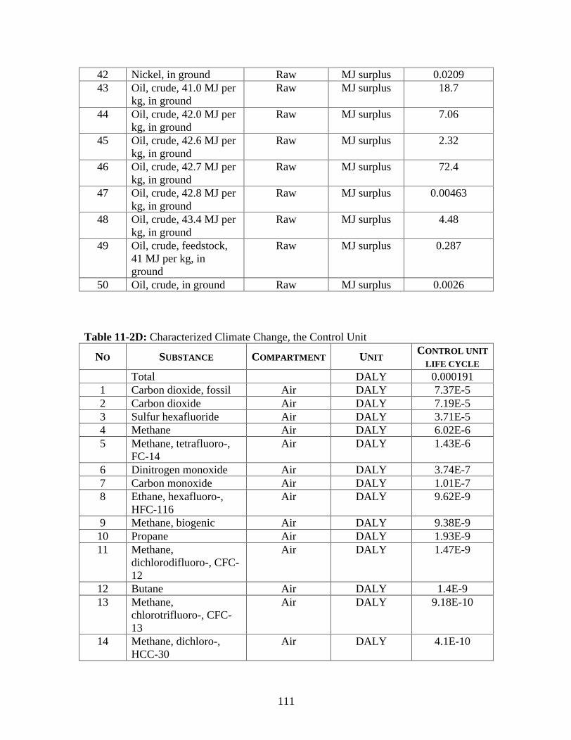
111
42 Nickel, in ground Raw MJ surplus 0.0209 43 Oil, crude, 41.0 MJ per
kg, in ground Raw MJ surplus 18.7
44 Oil, crude, 42.0 MJ per kg, in ground
Raw MJ surplus 7.06
45 Oil, crude, 42.6 MJ per kg, in ground
Raw MJ surplus 2.32
46 Oil, crude, 42.7 MJ per kg, in ground
Raw MJ surplus 72.4
47 Oil, crude, 42.8 MJ per kg, in ground
Raw MJ surplus 0.00463
48 Oil, crude, 43.4 MJ per kg, in ground
Raw MJ surplus 4.48
49 Oil, crude, feedstock, 41 MJ per kg, in ground
Raw MJ surplus 0.287
50 Oil, crude, in ground Raw MJ surplus 0.0026
Table 11-2D: Characterized Climate Change, the Control Unit
NO SUBSTANCE COMPARTMENT
UNIT CONTROL UNIT
LIFE CYCLE
Total DALY 0.000191 1 Carbon dioxide, fossil Air DALY 7.37E-5 2 Carbon dioxide Air DALY 7.19E-5 3 Sulfur hexafluoride Air DALY 3.71E-5 4 Methane Air DALY 6.02E-6 5 Methane, tetrafluoro-,
FC-14 Air DALY 1.43E-6
6 Dinitrogen monoxide Air DALY 3.74E-7 7 Carbon monoxide Air DALY 1.01E-7 8 Ethane, hexafluoro-,
HFC-116 Air DALY 9.62E-9
9 Methane, biogenic Air DALY 9.38E-9 10 Propane Air DALY 1.93E-9 11 Methane,
dichlorodifluoro-, CFC-12
Air DALY 1.47E-9
12 Butane Air DALY 1.4E-9 13 Methane,
chlorotrifluoro-, CFC-13
Air DALY 9.18E-10
14 Methane, dichloro-, HCC-30
Air DALY 4.1E-10

112
15 Methane,
trichlorofluoro-, CFC-11
Air DALY 2.27E-10
16 Ethane, 1,1,1,2-tetrafluoro-, HFC-134a
Air DALY 1.72E-10
17 Methane, fossil Air DALY 4.23E-11 18 Carbon monoxide,
fossil Air DALY 2.69E-11
19 Chloroform Air DALY 4.85E-16 20 Carbon monoxide,
biogenic Air DALY 2.91E-20
21 Methane, tetrachloro-, CFC-10
Air DALY -2.9E-11
22 Ethane, 1,1,1-trichloro-, HCFC-140
Air DALY -1.01E-9
23 Methane, bromotrifluoro-, Halon 1301
Air DALY -1.17E-8
24 Carbon dioxide, biogenic
Air DALY -4.53E-8
Table 11-2E: Characterized Fossil Fuels, Control Unit
NO SUBSTANCE COMPARTMENT
UNIT CONTROL UNIT
LIFE CYCLE
Total MJ surplus 629 1 Coal, 20.5 MJ per kg,
in ground Raw MJ surplus 245
2 Coal, 29.3 MJ per kg, in ground
Raw MJ surplus 170
3 Gas, natural, 50.3 MJ per kg, in ground
Raw MJ surplus 94.1
4 Oil, crude, 42.7 MJ per kg, in ground
Raw MJ surplus 72.4
5 Oil, crude, 41.0 MJ per kg, in ground
Raw MJ surplus 18.7
6 Oil, crude, 42.0 MJ per kg, in ground
Raw MJ surplus 7.06
7 Coal, 18 MJ per kg, in ground
Raw MJ surplus 4.71
8 Oil, crude, 43.4 MJ per kg, in ground
Raw MJ surplus 4.48
9 Oil, crude, 42.6 MJ per kg, in ground
Raw MJ surplus 2.32
10 Gas, natural, 36.6 MJ Raw MJ surplus 2.28

113
per m3, in ground
11 Coal, 22.1 MJ per kg, in ground
Raw MJ surplus 2.25
12 Gas, natural, 51.3 MJ per kg, in ground
Raw MJ surplus 1.19
13 Coal, brown, 10.0 MJ per kg, in ground
Raw MJ surplus 1.12
14 Coal, brown, 8.2 MJ per kg, in ground
Raw MJ surplus 1.06
15 Gas, natural, 35.9 MJ per m3, in ground
Raw MJ surplus 1.05
16 Gas, off-gas, 35.0 MJ per m3, oil production, in ground
Raw MJ surplus 0.934
17 Coal, 21.5 MJ per kg, in ground
Raw MJ surplus 0.314
18 Oil, crude, feedstock, 41 MJ per kg, in ground
Raw MJ surplus 0.287
19 Coal, brown, 8.1 MJ per kg, in ground
Raw MJ surplus 0.271
20 Coal, brown, 8 MJ per kg, in ground
Raw MJ surplus 0.218
21 Gas, natural, feedstock, 35 MJ per m3, in ground
Raw MJ surplus 0.16
22 Gas, natural, 35.0 MJ per m3, in ground
Raw MJ surplus 0.118
23 Energy, from gas, natural
Raw MJ surplus 0.114
24 Coal, 18.0 MJ per kg, in ground
Raw MJ surplus 0.0956
25 Coal, brown, 14.1 MJ per kg, in ground
Raw MJ surplus 0.0907
26 Coal, 18.5 MJ per kg, in ground
Raw MJ surplus 0.0746
27 Energy, from oil Raw MJ surplus 0.0669 28 Coal, 22.6 MJ per kg,
in ground Raw MJ surplus 0.0575
29 Coal, 13.3 MJ per kg, in ground
Raw MJ surplus 0.0261
30 Gas, natural, 35 MJ per m3, in ground
Raw MJ surplus 0.017
31 Coal, 28.0 MJ per kg, in ground
Raw MJ surplus 0.0162
32 Coal, 19.5 MJ per kg, Raw MJ surplus 0.0112

114
in ground
33 Energy, from coal Raw MJ surplus 0.0109 34 Oil, crude, 42.8 MJ per
kg, in ground Raw MJ surplus 0.00463
35 Gas, natural, feedstock, 35.0 MJ per m3, in ground
Raw MJ surplus 0.00421
36 Oil, crude, in ground Raw MJ surplus 0.0026 37 Energy, from coal,
brown Raw MJ surplus 0.00173
38 Coal, brown, 8.0 MJ per kg, in ground
Raw MJ surplus 0.000534
39 Coal, 24.0 MJ per kg, in ground
Raw MJ surplus -0.948
Table 11-2F: Characterization of Mineral resources, Control Unit
NO SUBSTANCE COMPARTMENT
UNIT CONTROL UNIT
LIFE CYCLE
Total MJ surplus 107 1 Copper, in ground Raw MJ surplus 104 2 Aluminum, in ground Raw MJ surplus 1.28 3 Bauxite, in ground Raw MJ surplus 0.816 4 Lead, in ground Raw MJ surplus 0.325 5 Iron ore, in ground Raw MJ surplus 0.18 6 Iron, in ground Raw MJ surplus 0.177 7 Nickel, in ground Raw MJ surplus 0.0209 8 Tin, in ground Raw MJ surplus 0.0061 9 Chromium, in ground Raw MJ surplus 0.00175
10 Manganese, in ground Raw MJ surplus 0.000272 11 Zinc, in ground Raw MJ surplus 0.000123 12 Molybdenum, in
ground Raw MJ surplus 2.94E-8
Table 11-2G: Characterized Respiratory Effects (in-organics) Control Unit
NO SUBSTANCE COMPARTMENT
UNIT CONTROL UNIT
LIFE CYCLE
Total DALY 0.00069 1 Sulfur dioxide Air DALY 0.000265 2 Nitrogen oxides Air DALY 0.000242 3 Sulfur oxides Air DALY 0.000132 4 Particulates, < 10 um Air DALY 3.84E-5 5 Nitrogen dioxide Air DALY 4.56E-6

115
6 Particulates Air DALY 4.51E-6 7 Particulates, SPM Air DALY 2.37E-6 8 Carbon monoxide Air DALY 2.3E-7 9 Ammonia Air DALY 2.13E-7
10 Nitric oxide Air DALY 1.59E-7 11 Particulates, < 2.5 um Air DALY 9.82E-8 12 Particulates, > 2.5 um,
and < 10um Air DALY 2.65E-8
13 Carbon monoxide, fossil
Air DALY 6.11E-11
14 Carbon monoxide, biogenic
Air DALY 6.61E-20
Table 11-2H: Characterized Environmental Load - Control Unit IMPACT CATEGORY UNIT CONTROL UNIT LIFE CYCLE
Carcinogens DALY 3.04E-5 Respiratory organics DALY 5.08E-7 Respiratory in-organics DALY 0.00069 Climate change DALY 0.000191 Radiation DALY x Ozone layer DALY 2.61E-8 Eco-toxicity PAF*m2yr 121 Acidification/ Eutrophication
PDF*m2yr 23.4
Land use PDF*m2yr 5.05 Minerals MJ surplus 107 Fossil fuels MJ surplus 629
Table 11-2I: Normalized Environmental Load per Impact Category - Control Unit IMPACT CATEGORY UNIT CONTROL UNIT LIFE CYCLE
Carcinogens 0.00197 Respiratory organics 3.29E-5 Respiratory in-organics 0.0446 Climate change 0.0123 Radiation x Ozone layer 1.69E-6 Eco-toxicity 0.00237 Acidification/ Eutrophication
0.00457
Land use 0.000984 Minerals 0.018 Fossil fuels 0.106

116
Table 11-2J: Weighted Environmental Load per Impact Category - Control Unit IMPACT CATEGORY UNIT CONTROL UNIT LIFE CYCLE
Total Pt 46.4 Carcinogens Pt 0.59 Respiratory organics Pt 0.00987 Respiratory in-organics Pt 13.4 Climate change Pt 3.7 Radiation Pt x Ozone layer Pt 0.000507 Eco-toxicity Pt 1.18 Acidification/ Eutrophication
Pt 2.28
Land use Pt 0.492 Minerals Pt 3.6 Fossil fuels Pt 21.1
Table 11-2K: Damage Assessment Results for the Control Unit DAMAGE CATEGORY UNIT CONTROL UNIT LIFE CYCLE
Human Health DALY 0.000911 Ecosystem Quality PDF*m2yr 40.6 Resources MJ surplus 736
Table 11-2L: Normalized Damage Assessment for the Control Unit DAMAGE CATEGORY UNIT CONTROL UNIT LIFE CYCLE
Human Health 0.0589 Ecosystem Quality 0.00792 Resources 0.124
Table 11-2M: Weighting of Damage Assessment for the Control Unit DAMAGE CATEGORY UNIT CONTROL UNIT LIFE CYCLE
Total Pt 46.4 Human Health Pt 17.7 Ecosystem Quality Pt 3.96 Resources Pt 24.7

117
11.3 CRT Monitor
Table 11-3A to 11-3P show the results obtained from the inventory results of the CRT monitor.
Table 11-3A: Damage Assessment to Ecosystem Quality
NO SUBSTANCE COMPARTMENT
UNIT CRT MONITOR
LIFE CYCLE
Total PDF*m2yr 56.9 1 Occupation, arable Raw PDF*m2yr 0.73
2 Occupation, construction site
Raw PDF*m2yr 0.0123
3 Occupation, forest Raw PDF*m2yr -0.0606 4 Occupation, industrial area Raw PDF*m2yr 0.248
5 Occupation, industrial area, vegetation
Raw PDF*m2yr 0.339
6 Occupation, mineral extraction site
Raw PDF*m2yr 0.00709
7 Occupation, traffic area Raw PDF*m2yr 3.68
8 Occupation, urban, continuously built
Raw PDF*m2yr 0.0626
9 Occupation, urban, green areas
Raw PDF*m2yr 0.0107
10 Transformation, from forest, intensive, clear-cutting
Raw PDF*m2yr 0.474
11 Transformation, from mineral extraction site
Raw PDF*m2yr -0.00696
12 Transformation, from unknown
Raw PDF*m2yr -2.8
13 Transformation, to arable Raw PDF*m2yr 2.68
14 Transformation, to industrial area
Raw PDF*m2yr 0.805
15 Transformation, to industrial area, vegetation
Raw PDF*m2yr 0.339
16 Transformation, to mineral extraction site
Raw PDF*m2yr 0.00696
17 Transformation, to shrub land, sclerophyllous
Raw PDF*m2yr 0.000912
18 Transformation, to urban, continuously built
Raw PDF*m2yr 1.48
19 Transformation, to water bodies, artificial
Raw PDF*m2yr 0.0622
20 Ammonia Air PDF*m2yr 0.0277

118
21 Arsenic Air PDF*m2yr 0.0409 22 Benzene Air PDF*m2yr 9.15E-7 23 Benzene, hexachloro- Air PDF*m2yr 6.87E-13 24 Benzo(a)pyrene Air PDF*m2yr 1.75E-5 25 Cadmium Air PDF*m2yr 0.0514 26 Chromium Air PDF*m2yr 0.424 27 Chromium-51 Air PDF*m2yr - 28 Chromium VI Air PDF*m2yr 0.117 29 Copper Air PDF*m2yr 0.0995
30 Dioxins, measured as 2,3,7,8-tetrachlorodibenzo-p-dioxin
Air PDF*m2yr 3.43E-6
31 Fluoranthene Air PDF*m2yr 5.52E-9 32 Heavy metals, unspecified Air PDF*m2yr -2.9E-8 33 Lead Air PDF*m2yr 1.07 34 Mercury Air PDF*m2yr 0.012 35 Metals, unspecified Air PDF*m2yr 0.0422 36 Nickel Air PDF*m2yr 0.929 37 Niobium-95 Air PDF*m2yr - 38 Nitric oxide Air PDF*m2yr 0.00389 39 Nitrogen dioxide Air PDF*m2yr 0.0732 40 Nitrogen oxides Air PDF*m2yr 28.2 41 Sulfur dioxide Air PDF*m2yr 5.74 42 Sulfur oxides Air PDF*m2yr 6.37 43 Zinc Air PDF*m2yr 0.251 44 Arsenic, ion Water PDF*m2yr 0.00128 45 Benzene Water PDF*m2yr 6.25E-7 46 Cadmium, ion Water PDF*m2yr 0.0197 47 Chromium Water PDF*m2yr 0.0255 48 Chromium VI Water PDF*m2yr 7.83E-6 49 Chromium, ion Water PDF*m2yr 5.69E-6 50 Copper, ion Water PDF*m2yr 5 51 DNOC Water PDF*m2yr -1.65E-10 52 Lead Water PDF*m2yr 0.0458 53 Mercury Water PDF*m2yr 4.66E-5 54 Metallic ions, unspecified Water PDF*m2yr 0.00192 55 Nickel, ion Water PDF*m2yr 0.136
56 PAH, polycyclic aromatic hydrocarbons
Water PDF*m2yr 5.14E-9
57 Phenol, pentachloro- Water PDF*m2yr -1.27E-8 58 Phthalate, dioctyl- Water PDF*m2yr 4.14E-13 59 Toluene Water PDF*m2yr 3.63E-6 60 Zinc, ion Water PDF*m2yr 0.0185 61 Arsenic Soil PDF*m2yr 0.000608 62 Cadmium Soil PDF*m2yr 0.00125

119
63 Chromium Soil PDF*m2yr 0.000229 64 Chromium VI Soil PDF*m2yr 0.00015 65 Copper Soil PDF*m2yr 0.00301 66 Lead Soil PDF*m2yr 3.25E-5 67 Mercury Soil PDF*m2yr 6.31E-5 68 Nickel Soil PDF*m2yr 0.0658 69 Zinc Soil PDF*m2yr 0.0114
Table 11-3B: Damage Assessment to Human Health
NO SUBSTANCE COMPARTMENT
UNIT
CRT MONITOR LIFE
CYCLE
Total DALY 0.00144 1 2-Propanol Air DALY 7.44E-11 2 Acetaldehyde Air DALY 1.57E-11 3 Acetic acid Air DALY 2.24E-11 4 Acetone Air DALY 8.71E-10 5 Acrolein Air DALY 9.72E-15 6 Acrylonitrile Air DALY 2.14E-9 7 Alcohols, unspecified Air DALY 1.33E-8 8 Aldehyde, unspecified Air DALY 2.19E-10 9 Ammonia Air DALY 1.51E-7
10 Arsenic Air DALY 1.7E-6 11 Benzaldehde Air DALY 2.72E-15 12 Benzene Air DALY 9.88E-10 13 Benzene, ethyl- Air DALY 1.32E-10 14 Benzene, hexachloro- Air DALY 1.46E-15 15 Benzene, pentachloro- Air DALY 9.91E-20 16 Benzo(a)pyrene Air DALY 4.91E-10 17 Butane Air DALY 8.22E-10 18 Butene Air DALY 7.26E-12 19 Cadmium Air DALY 7.19E-7 20 Carbon-14 Air DALY 1.37E-11 21 Carbon dioxide Air DALY 3.26E-5 22 Carbon dioxide, biogenic Air DALY -5.64E-8 23 Carbon dioxide, fossil Air DALY 0.000197 24 Carbon monoxide Air DALY 3.38E-7 25 Carbon monoxide,
biogenic Air DALY 2.82E-19
26 Carbon monoxide, fossil Air DALY 3.3E-10 27 Cesium-134 Air DALY 2.94E-16 28 Cesium-137 Air DALY 6.24E-16 29 Chloroform Air DALY 9.13E-14

120
30 Chromium VI Air DALY 1.65E-7 31 Cobalt-58 Air DALY 2.43E-19 32 Cobalt-60 Air DALY 1.98E-17 33 Cumene Air DALY 5.56E-12 34 Cyclohexane Air DALY 1.26E-11 35 Dinitrogen monoxide Air DALY 6.53E-7 35 Dioxins, measured as
2,3,7,8-tetrachlorodibenzo-p-dioxin
Air DALY 4.65E-9
37 Ethane Air DALY 5.51E-10 38 Ethane, 1,1,1-trichloro-,
HCFC-140 Air DALY 3.4E-10
39 Ethane, 1,1,1,2-tetrafluoro-, HFC-134a
Air DALY 5.09E-10
40 Ethane, 1,2-dichloro- Air DALY 2.38E-9 41 Ethane, 1,2-dichloro-
1,1,2,2-tetrafluoro-, CFC-114
Air DALY 2.16E-12
42 Ethane, hexafluoro-, HFC-116
Air DALY 1.29E-9
43 Ethanol Air DALY 1.39E-10 44 Ethene Air DALY 2.12E-10 45 Ethene, chloro- Air DALY 5.18E-12 46 Ethene, tetrachloro- Air DALY 1.33E-15 47 Ethyne Air DALY 5.23E-13 48 Fluorine Air DALY 5.42E-12 49 Formaldehyde Air DALY 1.11E-9 50 Formaldehyde (methyl
aldehyde) Air DALY -
51 furans Air DALY - 52 Heat, waste Air DALY - 53 Heavy metals,
unspecified Air DALY -7.93E-14
54 Helium Air DALY - 55 Heptane Air DALY 3.23E-11 56 Hexane Air DALY 1.96E-10 57 Hydrocarbons, aliphatic,
alkanes, unspecified Air DALY 1.03E-10
58 Hydrocarbons, aliphatic, alkenes, unspecified
Air DALY 1.5E-10
59 Hydrocarbons, aromatic Air DALY 1.66E-9 60 Hydrocarbons,
chlorinated Air DALY 3.63E-11
61 Hydrocarbons, Air DALY 3.76E-16

121
halogenated
62 Hydrocarbons, unspecified
Air DALY 1.96E-7
63 Hydrogen-3, Tritium Air DALY 5.45E-15 64 Iodine-129 Air DALY 1.77E-13 65 Iodine-131 Air DALY 1.6E-17 66 Iodine-133 Air DALY 6.95E-20 67 Krypton-85 Air DALY 4.52E-13 68 Lead-210 Air DALY 7.05E-16 69 Metals, unspecified Air DALY 1.15E-7 70 Methane Air DALY 5.01E-6 71 Methane, biogenic Air DALY 6.71E-9 72 Methane, bromotrifluoro-
, Halon 1301 Air DALY 4.27E-9
73 Methane, chlorodifluoro-, HCFC-22
Air DALY 2.01E-15
74 Methane, chlorotrifluoro-, CFC-13
Air DALY 1.78E-10
75 Methane, dichloro-, HCC-30
Air DALY 2.68E-10
76 Methane, dichlorodifluoro-, CFC-12
Air DALY 1.99E-8
77 Methane, dichlorofluoro-, HCFC-21
Air DALY 8.05E-13
78 Methane, fossil Air DALY 1.43E-10 79 Methane, tetrachloro-,
CFC-10 Air DALY 3.01E-11
80 Methane, tetrafluoro-, FC-14
Air DALY 2.01E-7
81 Methane, trichlorofluoro-, CFC-11
Air DALY 1.19E-8
82 Methanol Air DALY 5.3E-12 83 Methyl ethyl ketone Air DALY 1.82E-14 84 Nickel Air DALY 5.62E-9 85 Nitric oxide Air DALY 6.07E-8 86 Nitrogen dioxide Air DALY 1.14E-6 87 Nitrogen oxides Air DALY 0.000441 88 PAH, polycyclic
aromatic hydrocarbons Air DALY 4.1E-9
89 Particulates Air DALY 2.41E-6 90 Particulates, < 10 um Air DALY 0.000103 91 Pentane Air DALY 6.07E-10 92 Phenol Air DALY 5.59E-12 93 Phenol, pentachloro- Air DALY 5.5E-17

122
94 Plutonium-238 Air DALY 2.85E-21 95 Plutonium-alpha Air DALY 1.73E-16 96 Polonium-210 Air DALY 1E-15 97 Propane Air DALY 1.44E-9 98 Propene Air DALY 2.08E-9 99 Propionic acid Air DALY 2.8E-12
100 Radium-226 Air DALY 6.45E-16 101 Radon-222 Air DALY 1.11E-10 102 Styrene Air DALY 1.77E-14 103 Sulfur dioxide Air DALY 0.000301 104 Sulfur hexafluoride Air DALY 5.37E-6 105 Sulfur oxides Air DALY 0.000334 106 t-Butyl methyl ether Air DALY 2.74E-16 107 Thorium-230 Air DALY 1.03E-14 108 Toluene Air DALY 1.35E-9 109 Uranium-234 Air DALY 2.4E-14 110 Uranium-235 Air DALY 2.52E-16 111 Uranium-238 Air DALY 2.43E-15 112 VOC, volatile organic
compounds Air DALY 1.86E-8
113 Xenon-133 Air DALY 3E-16 114 Xenon-133m Air DALY 8.9E-20 115 Xylene Air DALY 8.42E-10 116 Acrylonitrile Water DALY -1.09E-13 117 Antimony-124 Water DALY 8.69E-17 118 Arsenic, ion Water DALY 7.37E-6 119 Benzo(a)pyrene Water DALY -6.85E-10 120 Cadmium, ion Water DALY 2.93E-6 121 Chloroform Water DALY -2.05E-15 122 Chromium VI Water DALY 9.42E-17 123 Cobalt-58 Water DALY 8.36E-17 124 Cobalt-60 Water DALY 9.64E-13 125 Ethane, 1,1,2-trichloro- Water DALY 1.95E-21 126 Ethane, 1,2-dichloro- Water DALY 1.02E-11 127 Ethane, hexachloro- Water DALY 2.14E-19 128 Ethene, chloro- Water DALY 3.6E-14 129 Ethene, tetrachloro- Water DALY 5.66E-19 130 Ethene, trichloro- Water DALY 1.54E-15 131 Manganese-54 Water DALY 9.37E-16 132 Metallic ions,
unspecified Water DALY 2.3E-7
133 Methane, dichloro-, HCC-30
Water DALY 1.26E-13
134 Methane, tetrachloro-, CFC-10
Water DALY 1.53E-15
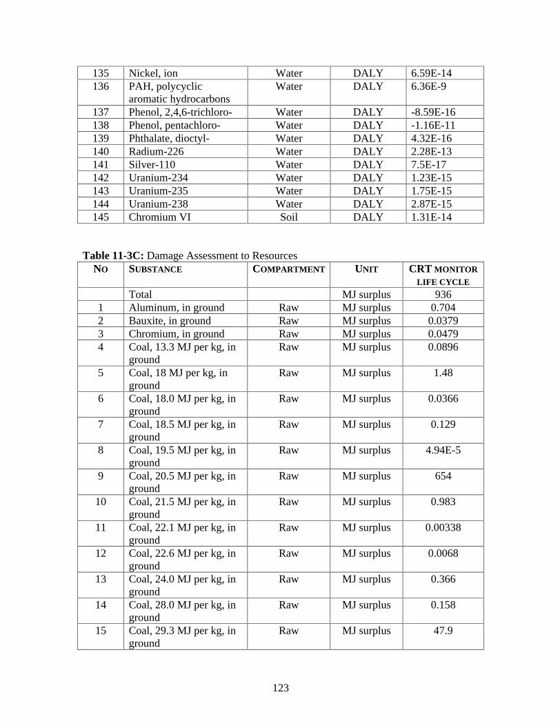
123
135 Nickel, ion Water DALY 6.59E-14 136 PAH, polycyclic
aromatic hydrocarbons Water DALY 6.36E-9
137 Phenol, 2,4,6-trichloro- Water DALY -8.59E-16 138 Phenol, pentachloro- Water DALY -1.16E-11 139 Phthalate, dioctyl- Water DALY 4.32E-16 140 Radium-226 Water DALY 2.28E-13 141 Silver-110 Water DALY 7.5E-17 142 Uranium-234 Water DALY 1.23E-15 143 Uranium-235 Water DALY 1.75E-15 144 Uranium-238 Water DALY 2.87E-15 145 Chromium VI Soil DALY 1.31E-14
Table 11-3C: Damage Assessment to Resources NO SUBSTANCE COMPARTMENT
UNIT CRT MONITOR
LIFE CYCLE
Total MJ surplus 936 1 Aluminum, in ground Raw MJ surplus 0.704 2 Bauxite, in ground Raw MJ surplus 0.0379 3 Chromium, in ground Raw MJ surplus 0.0479 4 Coal, 13.3 MJ per kg, in
ground Raw MJ surplus 0.0896
5 Coal, 18 MJ per kg, in ground
Raw MJ surplus 1.48
6 Coal, 18.0 MJ per kg, in ground
Raw MJ surplus 0.0366
7 Coal, 18.5 MJ per kg, in ground
Raw MJ surplus 0.129
8 Coal, 19.5 MJ per kg, in ground
Raw MJ surplus 4.94E-5
9 Coal, 20.5 MJ per kg, in ground
Raw MJ surplus 654
10 Coal, 21.5 MJ per kg, in ground
Raw MJ surplus 0.983
11 Coal, 22.1 MJ per kg, in ground
Raw MJ surplus 0.00338
12 Coal, 22.6 MJ per kg, in ground
Raw MJ surplus 0.0068
13 Coal, 24.0 MJ per kg, in ground
Raw MJ surplus 0.366
14 Coal, 28.0 MJ per kg, in ground
Raw MJ surplus 0.158
15 Coal, 29.3 MJ per kg, in ground
Raw MJ surplus 47.9

124
16 Coal, brown, 10 MJ per
kg, in ground Raw MJ surplus 0.413
17 Coal, brown, 14.1 MJ per kg, in ground
Raw MJ surplus 0.000399
18 Coal, brown, 8 MJ per kg, in ground
Raw MJ surplus 0.14
19 Coal, brown, 8.0 MJ per kg, in ground
Raw MJ surplus 0.000205
20 Coal, brown, 8.1 MJ per kg, in ground
Raw MJ surplus 0.879
21 Coal, brown, 8.2 MJ per kg, in ground
Raw MJ surplus 0.00468
22 Copper, in ground Raw MJ surplus 78 23 Energy, from coal Raw MJ surplus 0.0439 24 Energy, from coal, brown
Raw MJ surplus 0.00685 25 Energy, from gas, natural Raw MJ surplus 0.45 26 Energy, from oil Raw MJ surplus 0.265 27 Gas, mine, off-gas,
process, coal mining/kg Raw MJ surplus 4.13E-5
28 Gas, natural, 35 MJ per m3, in ground
Raw MJ surplus 0.0143
29 Gas, natural, 35.0 MJ per m3, in ground
Raw MJ surplus 0.0203
30 Gas, natural, 35.9 MJ per m3, in ground
Raw MJ surplus 4.3
31 Gas, natural, 36.6 MJ per m3, in ground
Raw MJ surplus 0.902
32 Gas, natural, 50.3 MJ per kg, in ground
Raw MJ surplus 1.26
33 Gas, natural, 51.3 MJ per kg, in ground
Raw MJ surplus 29.9
34 Gas, natural, feedstock, 35 MJ per m3, in ground
Raw MJ surplus 0.0306
35 Gas, off-gas, 35.0 MJ per m3, oil production, in ground
Raw MJ surplus 0.248
36 Gas, petroleum, 35 MJ per m3, in ground
Raw MJ surplus 0.00797
37 Iron ore, in ground Raw MJ surplus 0.0412 38 Iron, in ground Raw MJ surplus 0.0239 39 Lead, in ground Raw MJ surplus 9.29 40 Manganese, in ground Raw MJ surplus 0.000853 41 Molybdenum, in ground Raw MJ surplus 1.56E-8 42 Nickel, in ground Raw MJ surplus 0.23 43 Oil, crude, 41.0 MJ per Raw MJ surplus 0.486

125
kg, in ground
44 Oil, crude, 42.0 MJ per kg, in ground
Raw MJ surplus 26.1
45 Oil, crude, 42.6 MJ per kg, in ground
Raw MJ surplus 5.51
46 Oil, crude, 42.7 MJ per kg, in ground
Raw MJ surplus 52.2
47 Oil, crude, 42.8 MJ per kg, in ground
Raw MJ surplus 0.0172
48 Oil, crude, 43.4 MJ per kg, in ground
Raw MJ surplus 16.5
49 Oil, crude, feedstock, 41 MJ per kg, in ground
Raw MJ surplus 0.034
50 Oil, crude, in ground Raw MJ surplus 2.89 51 Zinc, in ground Raw MJ surplus 3.28E-5
Table 11-3D: Characterized mineral resources NO SUBSTANCE COMPARTMENT UNIT CRT MONITOR
LIFE CYCLE
Total MJ surplus 88.4 1 Aluminum, in ground Raw MJ surplus 0.704 2 Bauxite, in ground Raw MJ surplus 0.0379 3 Chromium, in ground Raw MJ surplus 0.0479 4 Copper, in ground Raw MJ surplus 78 5 Iron ore, in ground Raw MJ surplus 0.0412 6 Iron, in ground Raw MJ surplus 0.0239 7 Lead, in ground Raw MJ surplus 9.29 8 Manganese, in ground Raw MJ surplus 0.000853 9 Molybdenum, in ground Raw MJ surplus 1.56E-8
10 Nickel, in ground Raw MJ surplus 0.23 11 Zinc, in ground Raw MJ surplus 3.28E-5
Table 11-3E: Characterized Climate Change CRT Monitor NO SUBSTANCE COMPARTMENT UNIT CRT MONITOR
LIFE CYCLE
Total DALY 0.000241 1 Carbon dioxide Air DALY 3.26E-5 2 Carbon dioxide, biogenic Air DALY -5.64E-8 3 Carbon dioxide, fossil Air DALY 0.000197 4 Carbon monoxide Air DALY 1.04E-7 5 Carbon monoxide,
biogenic Air DALY 8.62E-20
6 Carbon monoxide, fossil Air DALY 1.01E-10

126
7 Chloroform Air DALY 2.82E-15 8 Dinitrogen monoxide Air DALY 6.53E-7 9 Ethane, 1,1,1-trichloro-,
HCFC-140 Air DALY -1.76E-10
10 Ethane, 1,1,1,2-tetrafluoro-, HFC-134a
Air DALY 5.09E-10
11 Ethane, CFC-114 Air DALY 1.53E-12 12 Ethane, hexafluoro-,
HFC-116 Air DALY 1.29E-9
13 Methane Air DALY 5E-6 14 Methane, biogenic Air DALY 6.69E-9 15 Methane, bromotrifluoro-
, Halon 1301 Air DALY -5.51E-9
16 Methane, chlorodifluoro-, HCFC-22
Air DALY 1.74E-15
17 Methane, chlorotrifluoro-, CFC-13
Air DALY 1.33E-10
18 Methane, dichloro-, HCC-30
Air DALY 2.06E-10
19 Methane, dichlorodifluoro-, CFC-12
Air DALY 1.23E-8
20 Methane, dichlorofluoro-, HCFC-21
Air DALY 4.1E-13
21 Methane, fossil Air DALY 1.43E-10 22 Methane, tetrachloro-,
CFC-10 Air DALY -4.26E-12
23 Methane, tetrafluoro-, FC-14
Air DALY 2.01E-7
24 Methane, trichlorofluoro-, CFC-11
Air DALY 2.07E-9
25 Sulfur hexafluoride Air DALY 5.37E-6
Table 11-3F: Characterized results on the use of fossil fuels NO SUBSTANCE COMPARTMENT UNIT CRT MONITOR
LIFE CYCLE
Total MJ surplus 848 1 Coal, 13.3 MJ per kg, in
ground Raw MJ surplus 0.0896
2 Coal, 18 MJ per kg, in ground
Raw MJ surplus 1.48
3 Coal, 18.0 MJ per kg, in ground
Raw MJ surplus 0.0366
4 Coal, 18.5 MJ per kg, in Raw MJ surplus 0.129

127
ground
5 Coal, 19.5 MJ per kg, in ground
Raw MJ surplus 4.94E-5
6 Coal, 20.5 MJ per kg, in ground
Raw MJ surplus 654
7 Coal, 21.5 MJ per kg, in ground
Raw MJ surplus 0.983
8 Coal, 22.1 MJ per kg, in ground
Raw MJ surplus 0.00338
9 Coal, 22.6 MJ per kg, in ground
Raw MJ surplus 0.0068
10 Coal, 24.0 MJ per kg, in ground
Raw MJ surplus 0.366
11 Coal, 28.0 MJ per kg, in ground
Raw MJ surplus 0.158
12 Coal, 29.3 MJ per kg, in ground
Raw MJ surplus 47.9
13 Coal, brown, 10 MJ per kg, in ground
Raw MJ surplus 0.413
14 Coal, brown, 14.1 MJ per kg, in ground
Raw MJ surplus 0.000399
15 Coal, brown, 8 MJ per kg, in ground
Raw MJ surplus 0.14
16 Coal, brown, 8.0 MJ per kg, in ground
Raw MJ surplus 0.000205
17 Coal, brown, 8.1 MJ per kg, in ground
Raw MJ surplus 0.879
18 Coal, brown, 8.2 MJ per kg, in ground
Raw MJ surplus 0.00468
19 Energy, from coal Raw MJ surplus 0.0439 20 Energy, from coal, brown
Raw MJ surplus 0.00685 21 Energy, from gas, natural Raw MJ surplus 0.45 22 Energy, from oil Raw MJ surplus 0.265 23 Gas, mine, off-gas,
process, coal mining/kg Raw MJ surplus 4.13E-5
24 Gas, natural, 35 MJ per m3, in ground
Raw MJ surplus 0.0143
25 Gas, natural, 35.0 MJ per m3, in ground
Raw MJ surplus 0.0203
26 Gas, natural, 35.9 MJ per m3, in ground
Raw MJ surplus 4.3
27 Gas, natural, 36.6 MJ per m3, in ground
Raw MJ surplus 0.902
28 Gas, natural, 50.3 MJ per kg, in ground
Raw MJ surplus 1.26

128
29 Gas, natural, 51.3 MJ per
kg, in ground Raw MJ surplus 29.9
30 Gas, natural, feedstock, 35 MJ per m3, in ground
Raw MJ surplus 0.0306
31 Gas, off-gas, 35.0 MJ per m3, oil production, in ground
Raw MJ surplus 0.248
32 Gas, petroleum, 35 MJ per m3, in ground
Raw MJ surplus 0.00797
33 Oil, crude, 41.0 MJ per kg, in ground
Raw MJ surplus 0.486
34 Oil, crude, 42.0 MJ per kg, in ground
Raw MJ surplus 26.1
35 Oil, crude, 42.6 MJ per kg, in ground
Raw MJ surplus 5.51
36 Oil, crude, 42.7 MJ per kg, in ground
Raw MJ surplus 52.2
37 Oil, crude, 42.8 MJ per kg, in ground
Raw MJ surplus 0.0172
38 Oil, crude, 43.4 MJ per kg, in ground
Raw MJ surplus 16.5
39 Oil, crude, feedstock, 41 MJ per kg, in ground
Raw MJ surplus 0.034
40 Oil, crude, in ground Raw MJ surplus 2.89
Table 11-3G: Characterized Results on the Extraction of Mineral Resources NO SUBSTANCE COMPARTMENT UNIT CRT MONITOR
LIFE CYCLE
Total MJ surplus 88.4 1 Aluminum, in ground Raw MJ surplus 0.704 2 Bauxite, in ground Raw MJ surplus 0.0379 3 Chromium, in ground Raw MJ surplus 0.0479 4 Copper, in ground Raw MJ surplus 78 5 Iron ore, in ground Raw MJ surplus 0.0412 6 Iron, in ground Raw MJ surplus 0.0239 7 Lead, in ground Raw MJ surplus 9.29 8 Manganese, in ground Raw MJ surplus 0.000853 9 Molybdenum, in ground Raw MJ surplus 1.56E-8
10 Nickel, in ground Raw MJ surplus 0.23 11 Zinc, in ground Raw MJ surplus 3.28E-5

129
Table 11-3H: Characterized Eco-toxicity CRT Monitor
NO SUBSTANCE COMPARTMENT UNIT CRT MONITOR
LIFE CYCLE
1 Total PAF*m2yr 83.8 2 Arsenic Air PAF*m2yr 0.409 3 Benzene Air PAF*m2yr 9.15E-6 4 Benzene, hexachloro Air PAF*m2yr 6.87E-12 5 Benzo(a)pyrene Air PAF*m2yr 0.000175 6 Cadmium Air PAF*m2yr 0.514 7 Chromium Air PAF*m2yr 4.24 8 Chromium VI Air PAF*m2yr 1.17 9 Copper Air PAF*m2yr 0.995
10 Dioxins Air PAF*m2yr 3.43E-5 11 Fluoranthene Air PAF*m2yr 5.52E-8 12 Heavy metals,
unspecified Air PAF*m2yr -2.9E-7
13 Lead Air PAF*m2yr 10.7 14 Mercury Air PAF*m2yr 0.12 15 Metals, unspecified Air PAF*m2yr 0.422 16 Nickel Air PAF*m2yr 9.29 17 Phenol, pentachloro- Air PAF*m2yr 1.01E-12 18 Toluene Air PAF*m2yr 2.38E-6 19 Zinc Air PAF*m2yr 2.51 20 Arsenic, ion Water PAF*m2yr 0.0128 21 Chromium Water PAF*m2yr 0.255 22 Chromium VI Water PAF*m2yr 7.83E-5 23 Chromium, ion Water PAF*m2yr 5.69E-5 24 Copper, ion Water PAF*m2yr 50 25 Fluoranthene Water PAF*m2yr -6.09E-8 26 Lead Water PAF*m2yr 0.458 27 Mercury Water PAF*m2yr 0.000466 28 Metallic ions,
unspecified Water PAF*m2yr 0.0192
29 Nickel, ion Water PAF*m2yr 1.36 30 PAH, polycyclic
aromatic hydrocarbons Water PAF*m2yr 5.14E-8
Table 11-3I: Characterized Acidification/Eutrophication CRT Monitor
NO SUBSTANCE COMPARTMENT UNIT CRT MONITOR
LIFE CYCLE
Total PDF*m2yr 40.5 1 Ammonia Air PDF*m2yr 0.0277 2 Nitric oxide Air PDF*m2yr 0.00389

130
3 Nitrogen dioxide Air PDF*m2yr 0.0732 4 Nitrogen oxides Air PDF*m2yr 28.2 5 Sulfur dioxide Air PDF*m2yr 5.74 6 Sulfur oxides Air PDF*m2yr 6.37
Table 11-3J: Characterized Respiratory Effects (in-organics) CRT Monitor
NO SUBSTANCE COMPARTMENT UNIT CRT MONITOR
LIFE CYCLE
Total DALY 0.00118 1 Carbon monoxide Air DALY 2.35E-7 2 Carbon monoxide,
biogenic Air DALY 1.96E-19
3 Carbon monoxide, fossil Air DALY 2.29E-10 4 Nitric oxide Air DALY 6.07E-8 5 Nitrogen dioxide Air DALY 1.14E-6 6 Nitrogen oxides Air DALY 0.000441 7 Particulates Air DALY 2.41E-6 8 Particulates, < 10 um Air DALY 0.000103 9 Particulates, < 10 um
(mobile) Air DALY 4.54E-8
10 Particulates, < 10 um (stationary)
Air DALY 2.93E-9
11 Particulates, < 2.5 um Air DALY 3.16E-7 12 Particulates, > 2.5 um,
and < 10um Air DALY 9.15E-8
13 Particulates, SPM Air DALY 1.18E-6 14 Sulfur dioxide Air DALY 0.000301 15 Sulfur oxides Air DALY 0.000334
Table 11-3K: Characterized Environmental Load per impact category - CRT monitor IMPACT CATEGORY UNIT CRT MONITOR LIFE CYCLE
Carcinogens DALY 1.33E-5 Respiratory organics DALY 3.54E-7 Respiratory in-organics DALY 0.00118 Climate change DALY 0.000241 Radiation DALY 1.35E-10 Ozone layer DALY 2.78E-8 Eco-toxicity PAF*m2yr 83.8 Acidification/ Eutrophication
PDF*m2yr 40.5
Land use PDF*m2yr 8.07 Minerals MJ surplus 88.4 Fossil fuels MJ surplus 848

131
Table 11-3L: Normalized Environmental Load per Impact Category IMPACT CATEGORY UNIT CRT MONITOR LIFE CYCLE
Carcinogens 0.000858 Respiratory organics 2.29E-5 Respiratory in-organics 0.0766 Climate change 0.0156 Radiation 8.71E-9 Ozone layer 1.8E-6 Eco-toxicity 0.00163 Acidification/ Eutrophication
0.00789
Land use 0.00157 Minerals 0.0149 Fossil fuels 0.142
Table 11-3M: Weighting Environmental Load per Impact Category CRT Monitor IMPACT CATEGORY UNIT CRT MONITOR LIFE CYCLE
Total Pt 64.9 Carcinogens Pt 0.258 Respiratory organics Pt 0.00688 Respiratory in-organics Pt 23 Climate change Pt 4.68 Radiation Pt 2.61E-6 Ozone layer Pt 0.00054 Eco-toxicity Pt 0.817 Acidification/ Eutrophication
Pt 3.95
Land use Pt 0.787 Minerals Pt 2.97 Fossil fuels Pt 28.5
Table 11-3N: Damage Assessment Results CRT Monitor DAMAGE CATEGORY UNIT CRT MONITOR LIFE CYCLE
Human Health DALY 0.00144 Ecosystem Quality PDF*m2yr 56.9 Resources MJ surplus 936
Table 11-3O: Normalized Damage Assessment for the CRT Monitor DAMAGE CATEGORY UNIT CRT MONITOR LIFE CYCLE
Human Health 0.0931 Ecosystem Quality 0.0111 Resources 0.157

132
Table 11-3P: Damage Assessment on a weighted scale CRT Monitor DAMAGE CATEGORY UNIT CRT MONITOR LIFE CYCLE
Total Pt 64.9 Human Health Pt 27.9 Ecosystem Quality Pt 5.55 Resources Pt 31.5

133
12 Appendix C
Table 12-1 and figure 12-1 show the material composition for CRT monitor and the whole PC respectively. This data was used as a guide in the data that was already constructed after disassembling the PC system
Table 12-1: Product Composition in 17-inch CRT Monitor Material Weight (g) Weight %
Aluminum 48.55 0.33 Copper 892.15 6.09 Ferro 1324.08 9.04 Glass 9392.50 64.1 Plastics 2606.62 17.8 Ag 0.16 11 ppm Au 0.01 0.7 ppm Pd 0.00 0.33 ppm Other 385.22 2.63 Total 14649.30 100 (Source: Huisman J. et al. 2004, Eco-Efficiency Considerations on the End-of-life of consumer Electronic Products).

134
Material Composition of a PC
Plastics23%
Copper7%
Silica/glass26%
Ferrous metal20%
Zinc2%
Aluminum14%
Mercury0%
Cadmium0%
Lead6%
Other2%
Figure 12-1: shows the material composition of a personal computer (Source: Microelectronics and Computer Technology Corporation (MCC), 1996. Electronics Industry Environmental Roadmap. Austin, TX).

This document was created with Win2PDF available at http://www.daneprairie.com.The unregistered version of Win2PDF is for evaluation or non-commercial use only.
Top Related