


Languages
Pages
Legal

8/6/2019 Lecture13 Regression
http://slidepdf.com/reader/full/lecture13-regression 1/54
Linear Regression II

8/6/2019 Lecture13 Regression
http://slidepdf.com/reader/full/lecture13-regression 2/54
Linear regression
� An estimate of the linear relationshipbetween two variables (X & Y) interms of the actual scale
±We find the equation for the line thatbest fits the data
± This involves
�
Finding the intercept± e.g., the value of Ywhen X = 0
� Finding the slope± the change in Y given aone point change in X

8/6/2019 Lecture13 Regression
http://slidepdf.com/reader/full/lecture13-regression 3/54
Equation of a line
� Y¶ = a + bX
� The intercept (a) is the point at
which the line crosses the Y axis ± The value of Y when X = 0
� The slope (b) is the amount of
increase in Y given an increase inone point of X
� Y¶ means ³predicted Y value´

8/6/2019 Lecture13 Regression
http://slidepdf.com/reader/full/lecture13-regression 4/54
Making predictions
� We use the regression equation topredict what Y will be given some valueof X ± E.g., how tall is someone who weights 121
lbs?
� Last time, we focused on ³perfectpredictions´ ± Weight ³perfectly predicted´ height because
the correlation was one«
± That¶s usually not the case in real life«
8/6/2019 Lecture13 Regression
http://slidepdf.com/reader/full/lecture13-regression 5/54

8/6/2019 Lecture13 Regression
http://slidepdf.com/reader/full/lecture13-regression 6/54
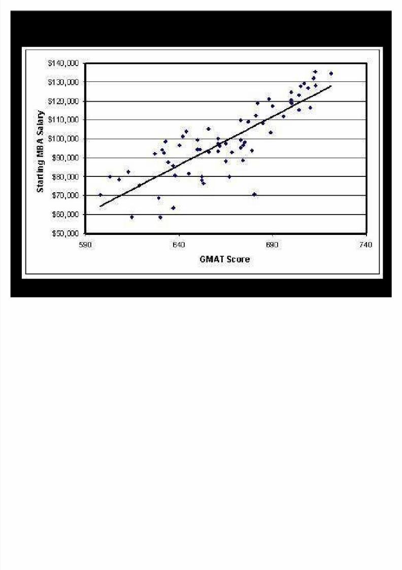
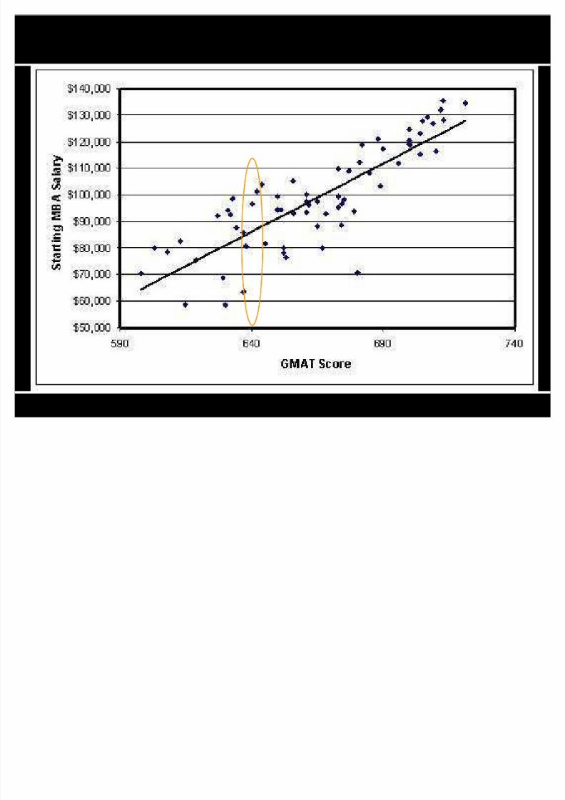
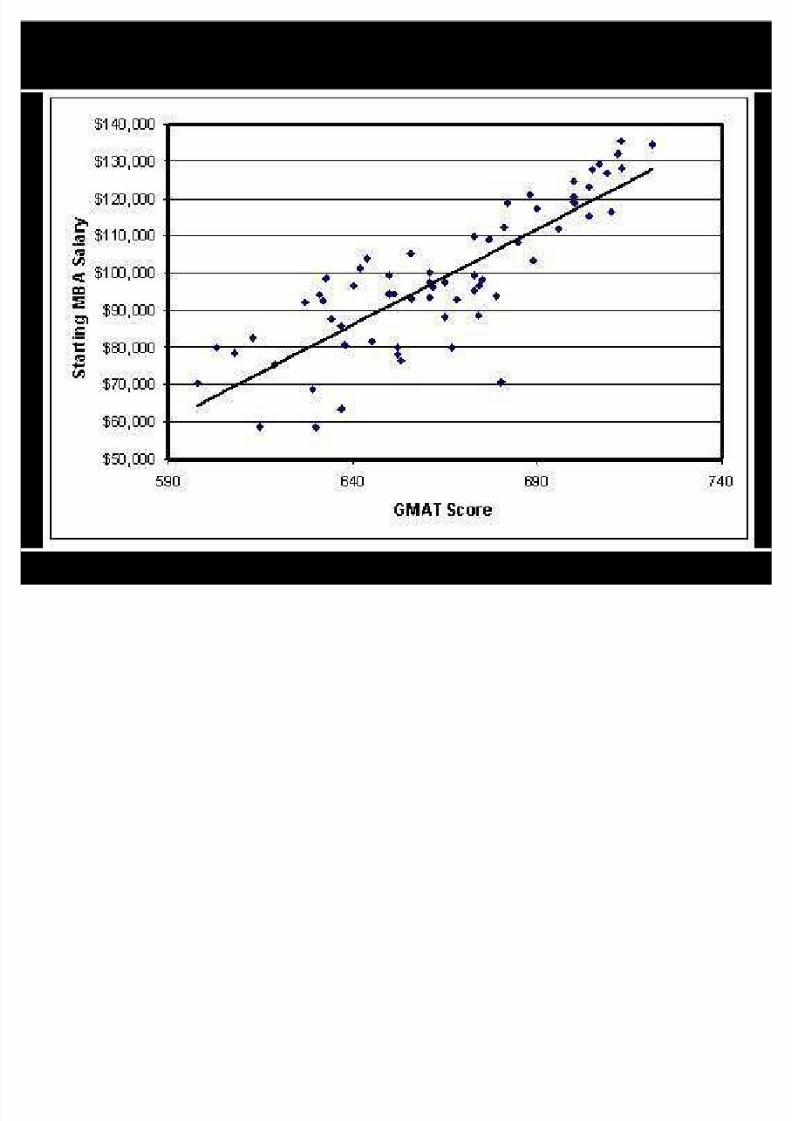
Making predictions
� One way to think about theregression line is in terms of
³conditional´ averages (means) ± Given some condition of X, what is the
mean of Y?
± So, given a GMAT score of 640, what is
the average income?
8/6/2019 Lecture13 Regression
http://slidepdf.com/reader/full/lecture13-regression 7/54

8/6/2019 Lecture13 Regression
http://slidepdf.com/reader/full/lecture13-regression 8/54
The line that ³best fits´
� The method behind linear regressioninvolves finding the line that ³best
fits´ the data ±We won¶t get into how this is computed
in this class
� Involves matrix algebra
± But conceptually, the point is to find aline that minimizes the total distancefrom all the points

8/6/2019 Lecture13 Regression
http://slidepdf.com/reader/full/lecture13-regression 9/54
The line that ³best fits´
� The method behind linear regressioninvolves finding the line that ³best fits´ the data ± We won¶t get into how this is computed in
this class� Involves matrix algebra
± But conceptually, the goal is to find a linethat minimizes the total distance from allthe points� Often called ³Ordinary Least Squares regression´
because you square the distance from eachpoint to the line and use an iterative process tominimize it± i.e., find the ³least´ amount of summed squares

8/6/2019 Lecture13 Regression
http://slidepdf.com/reader/full/lecture13-regression 10/54

8/6/2019 Lecture13 Regression
http://slidepdf.com/reader/full/lecture13-regression 11/54

8/6/2019 Lecture13 Regression
http://slidepdf.com/reader/full/lecture13-regression 12/54
Residuals
� The regression line is what we wouldpredict for Y given some X«

8/6/2019 Lecture13 Regression
http://slidepdf.com/reader/full/lecture13-regression 13/54

8/6/2019 Lecture13 Regression
http://slidepdf.com/reader/full/lecture13-regression 14/54
Residuals
� The regression line is what we wouldpredict for Y given some X« ± Regression equation gives us the straight
line that minimizes the error involved inmaking predictions
� Residuals are what we call error ± Residuals are the differences between an
actual Y value and the predicted Y value ± The residual is Y ± Y¶
� The actual Y value minus the predicted Y value

8/6/2019 Lecture13 Regression
http://slidepdf.com/reader/full/lecture13-regression 15/54
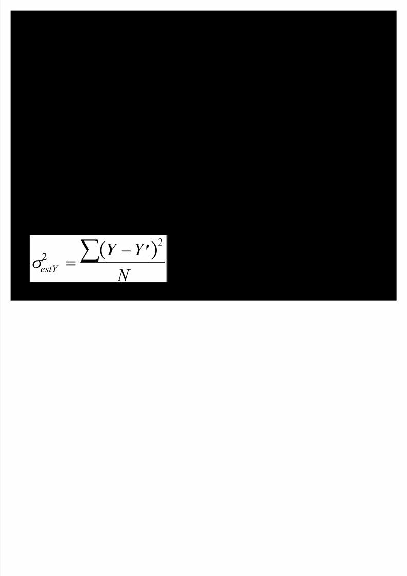
Variance of the estimate
� We can quantify the amount of errorin the prediction by finding theaverage of all of the square residuals

8/6/2019 Lecture13 Regression
http://slidepdf.com/reader/full/lecture13-regression 16/54
10000-11000

8/6/2019 Lecture13 Regression
http://slidepdf.com/reader/full/lecture13-regression 17/54
Variance of the estimate
� We can quantify the amount of errorin the prediction by finding theaverage of all of the squaredresiduals
± This is the ³variance of the estimate´ E.g., How much do the points vary
around the line
W estY
2 !Y dY
2
§ N
The closer thepoints are to theline, the smallerthe variance of the
estimate will be
8/6/2019 Lecture13 Regression
http://slidepdf.com/reader/full/lecture13-regression 18/54
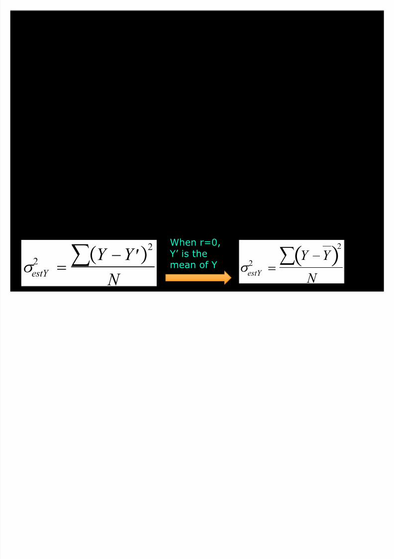
Variance of the Estimate
� When r=0 (no correlation), thismeans the best fitting line is ahorizontal one«
W estY
2 !Y dY
2
§ N
8/6/2019 Lecture13 Regression
http://slidepdf.com/reader/full/lecture13-regression 19/54
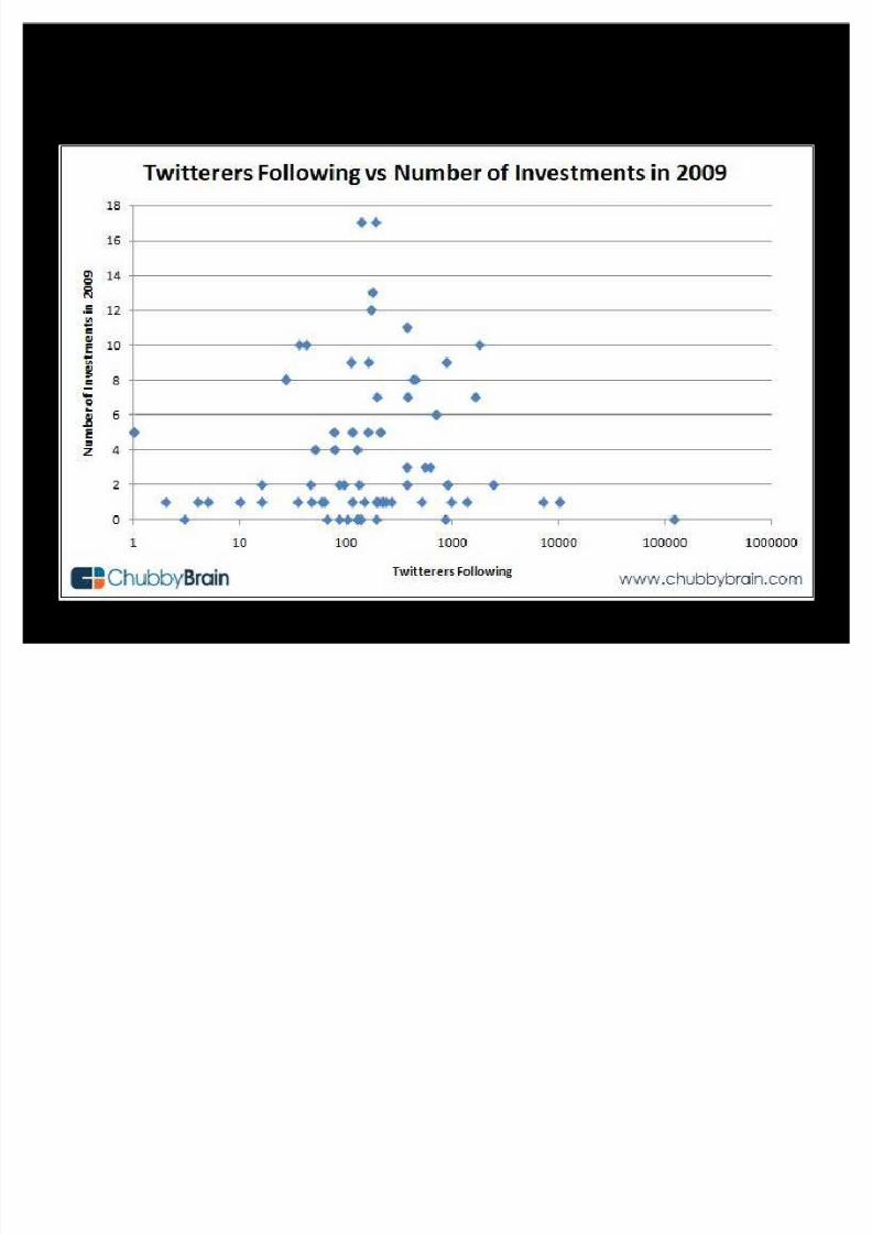
No correlation
8/6/2019 Lecture13 Regression
http://slidepdf.com/reader/full/lecture13-regression 20/54
No correlation
8/6/2019 Lecture13 Regression
http://slidepdf.com/reader/full/lecture13-regression 21/54
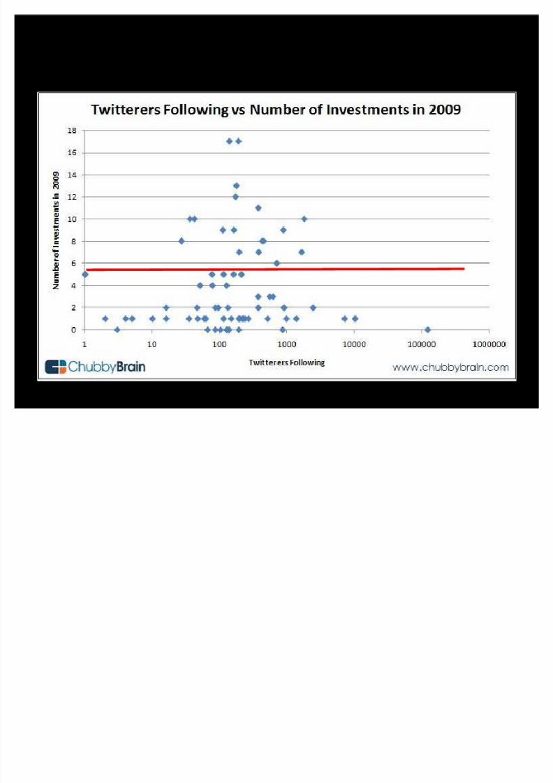
Variance of the Estimate� W
hen r=0 (no correlation), thismeans the best fitting line is ahorizontal one«
± Same predicted Y for all values of X
� The line is doing nothing for us..
± The variance of the estimate is largestin this case
� The variance of the predictions around theregression line is just the variance of Y
estY
2!
Y Y 2
§
N
W estY
2 !Y dY
2
§ N
When r=0,Y¶ is themean of Y

8/6/2019 Lecture13 Regression
http://slidepdf.com/reader/full/lecture13-regression 22/54
Variance of the estimate
� For a sample, we use N-2 in thedenominator to get an unbiasedestimate
± Two degrees of freedom
sest
2! Y
dY
2
§ N 2
8/6/2019 Lecture13 Regression
http://slidepdf.com/reader/full/lecture13-regression 23/54
Explained vs. unexplained
variance� The difference between the total
amount of variance in Y and thevariance of the estimate is theamount of v ariance explained by theregression line
� Explained variance = total variance-
unexplained variance ± Total Variance = Unexplained variance +Explained Variance
8/6/2019 Lecture13 Regression
http://slidepdf.com/reader/full/lecture13-regression 24/54
8/6/2019 Lecture13 Regression
http://slidepdf.com/reader/full/lecture13-regression 25/54
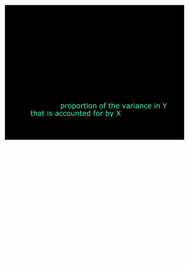
Coefficient of determination
� This is the ³proportion of the totalvariance that is explained (ordetermined) by the predictor
variable´ � It is the (explained variance)/(total
variance) ±
This equals r2
± It is the proportion of the variance in Ythat is accounted for by X

8/6/2019 Lecture13 Regression
http://slidepdf.com/reader/full/lecture13-regression 26/54
Coefficient of non-determination
� This is simply the reverse²theamount of variance in Y that X does
not account for ± An estimate of how much the points
don¶t fall on the line
�
It is the (unexplainedvariance)/(total variance) or (1-r2)
8/6/2019 Lecture13 Regression
http://slidepdf.com/reader/full/lecture13-regression 27/54
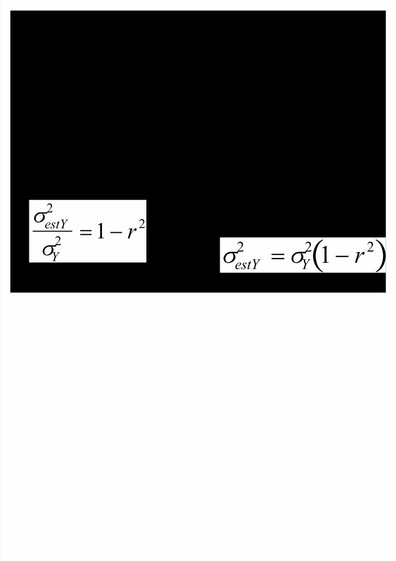
The variance of the
estimate� Remember that the variance of the
estimate is the unexplained variance
�
An easier way to compute thevariance of the estimate is to use thecoefficient of non-determination
estY 2
W Y
2!1 r 2
W estY
2! W
Y
2 1 r 2
Becomes«

8/6/2019 Lecture13 Regression
http://slidepdf.com/reader/full/lecture13-regression 28/54
Example
� Relationship between age and verbalcomprehension
� We want to use age (in months) topredict test scores on a verbalcomprehension test

8/6/2019 Lecture13 Regression
http://slidepdf.com/reader/full/lecture13-regression 29/54
Example
� In our sample of 100 kids fromgrades 1-6, we have
� Mean age of 98.14 months (s = 21.0)
� Mean test score of 30.35 items correctout of 50 (s = 7.25)
8/6/2019 Lecture13 Regression
http://slidepdf.com/reader/full/lecture13-regression 30/54
Example�
In our sample of 100 kids fromgrades 1-6, we have
� Mean age of 98.14 months (s = 21.0)
� Mean test score of 30.35 items correctout of 50 (s = 7.25)
Why use regression?Our independent variable is
age²a continuous measure«We don¶t have 2 groups tocompare, so we can use a t-test.We want to look at how increasesin age relate to increases (or
decreases) in scores

8/6/2019 Lecture13 Regression
http://slidepdf.com/reader/full/lecture13-regression 31/54
Example
� In our sample of 100 kids from grades1-6, we have
�
Mean age of 98.14 months (s = 21.0)� Mean test score of 30.35 items correct
out of 50 (s = 7.25)
� We find that the correlation between age
and test score in our sample is r = .72
� How can we make predictions forverbal comprehension given an age?

8/6/2019 Lecture13 Regression
http://slidepdf.com/reader/full/lecture13-regression 32/54
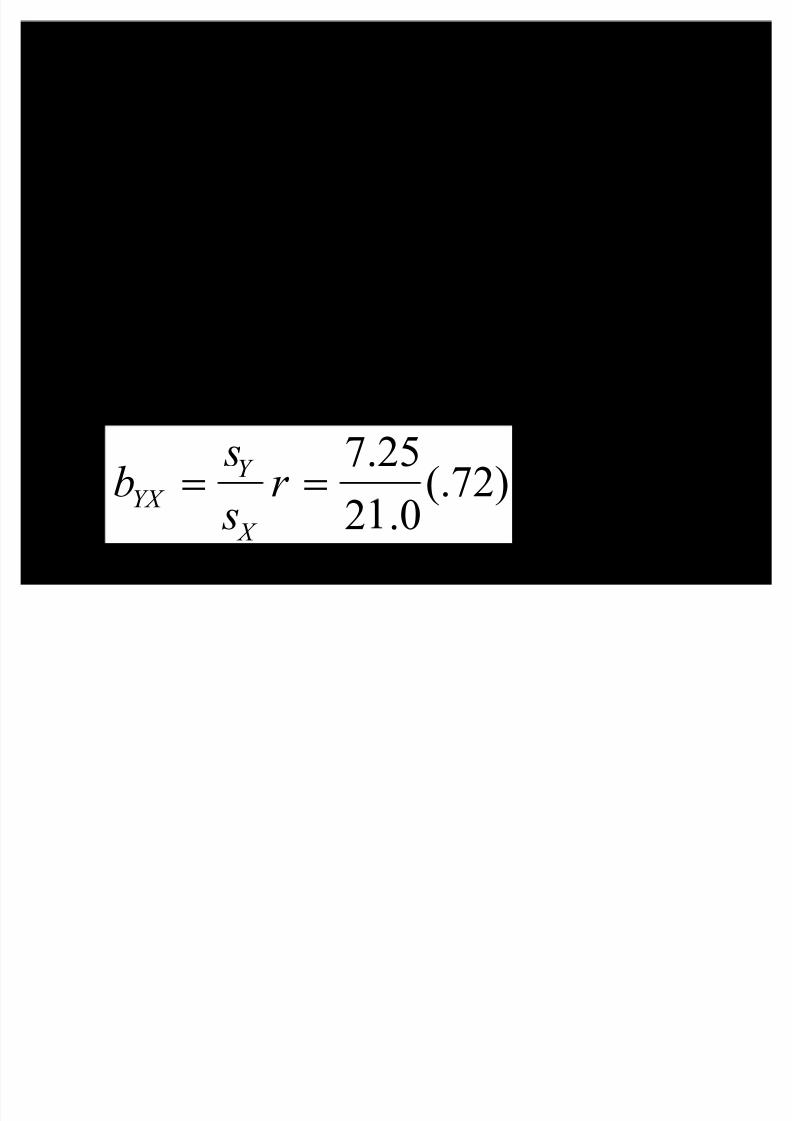
1. Find the slope of the line
� X is age (the independent variable)
±Mx = 98.14, sx = 21.0
� Y is test score (the dependent
variable)
±My = 30.35, sy = 7.25
� r = .72
bYX ! sY
s X
r
8/6/2019 Lecture13 Regression
http://slidepdf.com/reader/full/lecture13-regression 33/54
1. Find the slope of the line
� X is age (the independent variable)
±Mx = 98.14, sx = 21.0
� Y is test score (the dependent
variable)
±My = 30.35, sy = 7.25
� r = .72
bYX ! sY
s X
r !7.25
2 .0(.72)

8/6/2019 Lecture13 Regression
http://slidepdf.com/reader/full/lecture13-regression 34/54
1. Find the slope of the line
� X is age (the independent variable)
±Mx = 98.14, sx = 21.0
� Y is test score (the dependent
variable)
±My = 30.35, sy = 7.25
� r = .72
bYX ! sY
s X
r !7.25
2 .0(.72) ! .249
8/6/2019 Lecture13 Regression
http://slidepdf.com/reader/full/lecture13-regression 35/54
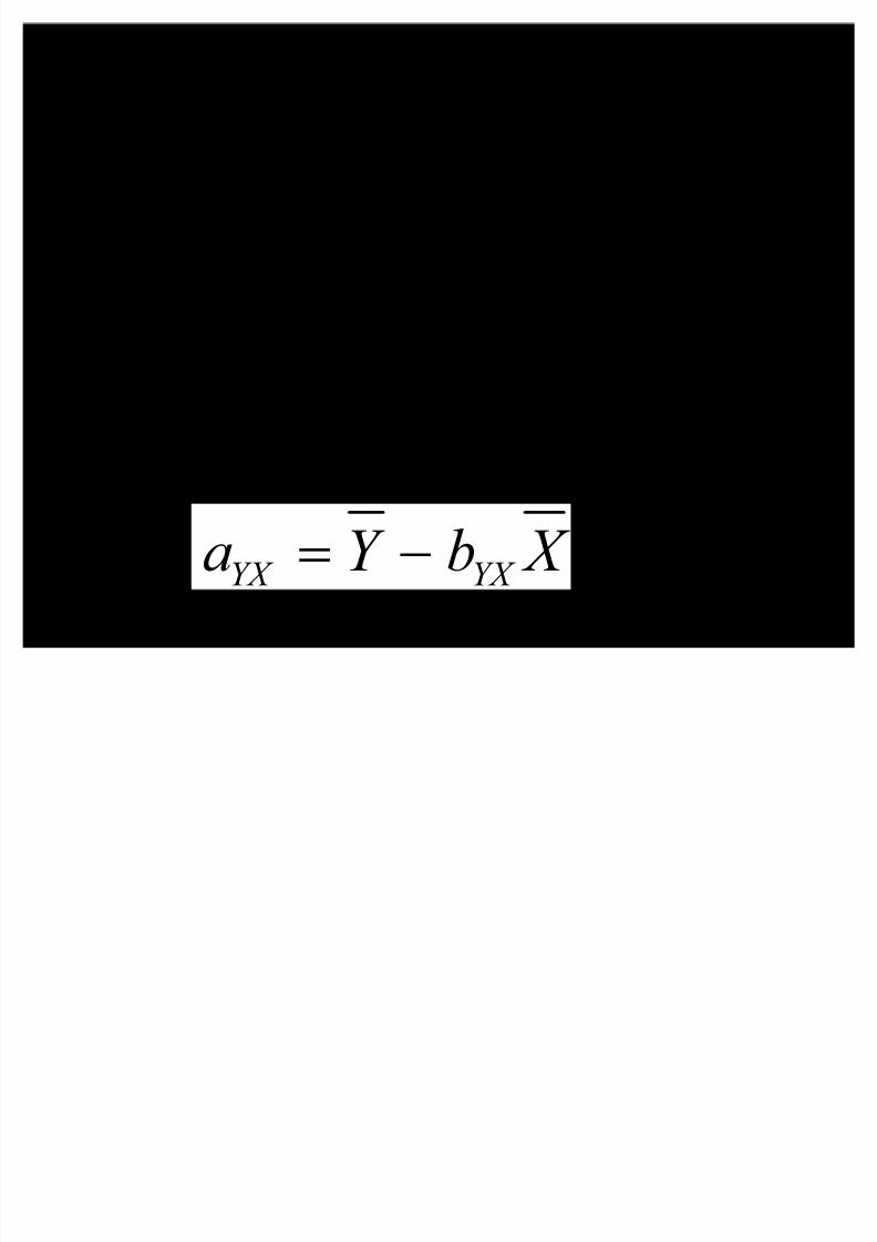
2. Find the intercept of the line
� X is age (the independent variable)
±Mx = 98.14, sx = 21.0
� Y is test score (the dependent
variable)
±My = 30.35, sy = 7.25
� b = .249
aYX
! Y bYX X

8/6/2019 Lecture13 Regression
http://slidepdf.com/reader/full/lecture13-regression 36/54
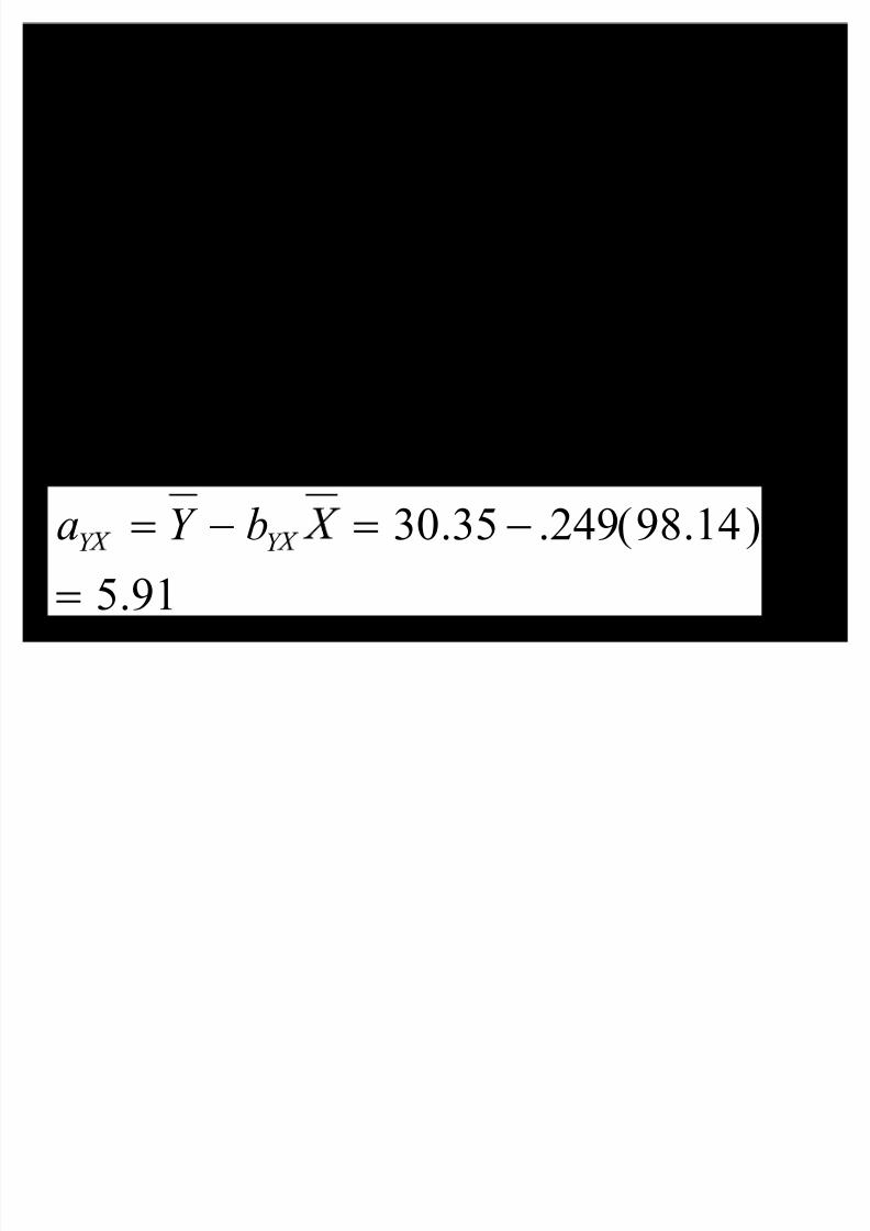
2. Find the intercept of the line
� X is age (the independent variable)
±Mx = 98.14, sx = 21.0
� Y is test score (the dependent
variable)
±My = 30.35, sy = 7.25
� b = .249
aYX
! Y bYX X ! 30.35 .249(98.14)
8/6/2019 Lecture13 Regression
http://slidepdf.com/reader/full/lecture13-regression 37/54
2. Find the intercept of the line
� X is age (the independent variable)
±Mx = 98.14, sx = 21.0
� Y is test score (the dependent
variable)
±My = 30.35, sy = 7.25
� b = .249
aY ! Y b
Y ! 30.35 .249(98.14)
!5
.9
1
8/6/2019 Lecture13 Regression
http://slidepdf.com/reader/full/lecture13-regression 38/54
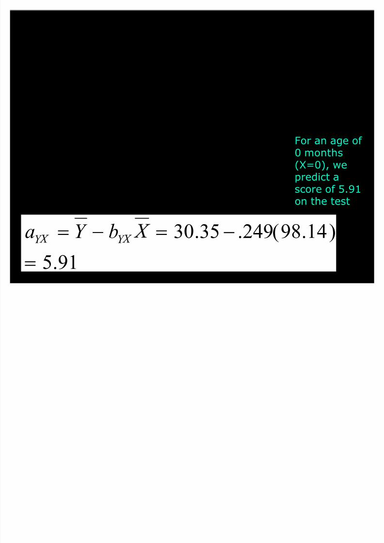
2. Find the intercept of the line
� X is age (the independent variable)
±Mx = 98.14, sx = 21.0
� Y is test score (the dependent
variable)
±My = 30.35, sy = 7.25
� b = .249
aY ! Y b
Y ! 30.35 .249(98.14)
!5
.9
1
For an age of 0 months(X=0), wepredict ascore of 5.91
on the test

8/6/2019 Lecture13 Regression
http://slidepdf.com/reader/full/lecture13-regression 39/54
Making a prediction
� Y¶ = a + bX ± a = 5.91
± b = .249
� Y¶ means ³predicted Y´
� A child is 10 years old (120 months) ± His predicted test result will be:Y¶ = 5.91 + .249(120) = 35.8 items
correct
8/6/2019 Lecture13 Regression
http://slidepdf.com/reader/full/lecture13-regression 40/54
Example�
In our sample of 100 kids fromgrades 1-6, we have
� Mean age of 98.14 months (s = 21.0)
� Mean test score of 30.35 items correctout of 50 (s = 7.25)
We predict a child at 120months will get 35.8 items
correctThis child is older than theaverage child in our sample,so he does better than
average on the test

8/6/2019 Lecture13 Regression
http://slidepdf.com/reader/full/lecture13-regression 41/54
Interpreting: r vs. b
� b (the slope of the line) is the change(amount of points) we predict in Ybased on a one point change is X ± For each month increase in age, test scores
go up .249
� r (the correlation) is the change (interms of standard deviations) wepredict in Y based on a one standard
deviation change in X ± For every one standard deviation increase
in age, test scores will increase by .72 of astandard deviation

8/6/2019 Lecture13 Regression
http://slidepdf.com/reader/full/lecture13-regression 42/54
The residual
� Our equation is:
Test score = 5.91 + .249(age in months)
� We have a child who is 92 months old,
and she gets 40 questions correct
� We¶d predict she would get
Y¶ =5.91+.249(92) = 28.82 questions
correct
8/6/2019 Lecture13 Regression
http://slidepdf.com/reader/full/lecture13-regression 43/54
The residual
� Our equation is:Test score = 5.91 + .249(age in months)
� We have a child who is 92 months old,
and she gets 40 questions correct� We¶d predict she would get
Y¶ =5.91+.249(92) = 28.82 questionscorrect
The residual is 40-28.82 = 11.18
Positive because she did better thanour predicted value
8/6/2019 Lecture13 Regression
http://slidepdf.com/reader/full/lecture13-regression 44/54
The residual
� Our equation is:Test score = 5.91 + .249(age in months)
� We have a child who is 92 months old, and shegets 40 questions correct
� We¶d predict she would get
Y¶ =5.91+.249(92) = 28.82 questions correct
The residual is 40-28.82 = 11.18
Positive because she did better than ourpredicted value
If another 92 month old got 27 questionscorrect, the residual would be 27-28.82=-1.12

8/6/2019 Lecture13 Regression
http://slidepdf.com/reader/full/lecture13-regression 45/54
Example: Variance explained
�
In our sample of 100 kids fromgrades 1-6, we have
� Mean age of 98.14 months (s = 21.0)
� Mean test score of 30.35 items correctout of 50 (s = 7.25)
The total variance in testscores is s2 = 7.252 = 52.56
How much is explained bythe regression line?
8/6/2019 Lecture13 Regression
http://slidepdf.com/reader/full/lecture13-regression 46/54
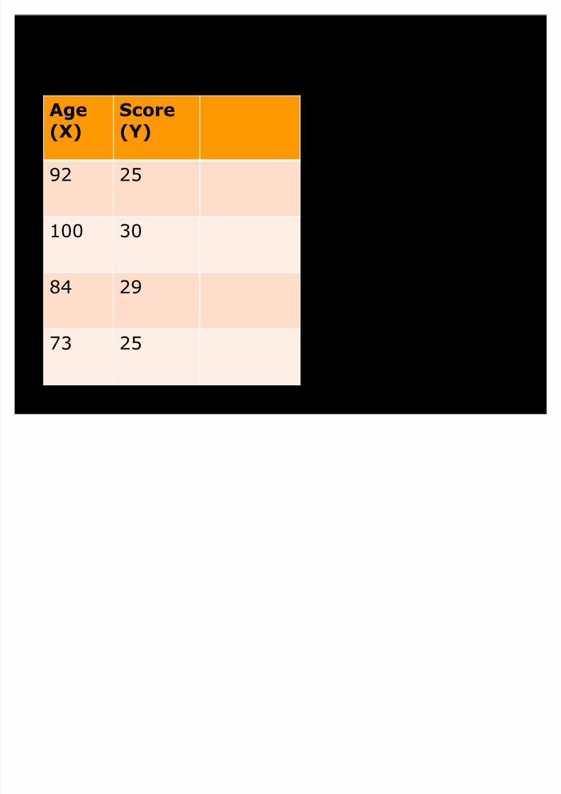
Unexplained variance
� If we went through each of our 100data points, we could calculate theresidual± the value of Y we actuallygot minus the value of Y wepredicted from the equation
± The sum of those squared deviations is
everything we didn¶t explain
Y Y '
2
§
8/6/2019 Lecture13 Regression
http://slidepdf.com/reader/full/lecture13-regression 47/54
Age(X)
Score(Y)
92 25
100 30
84 29
73 25
8/6/2019 Lecture13 Regression
http://slidepdf.com/reader/full/lecture13-regression 48/54
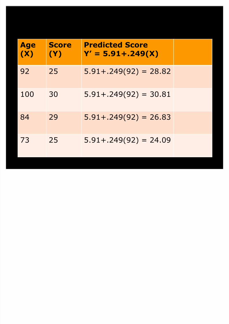
Age(X)
Score(Y)
Predicted ScoreY¶ = 5.91+.249(X)
92 25 5.91+.249(92) = 28.82
100 30 5.91+.249(92) = 30.81
84 29 5.91+.249(92) = 26.83
73 25 5.91+.249(92) = 24.09
8/6/2019 Lecture13 Regression
http://slidepdf.com/reader/full/lecture13-regression 49/54
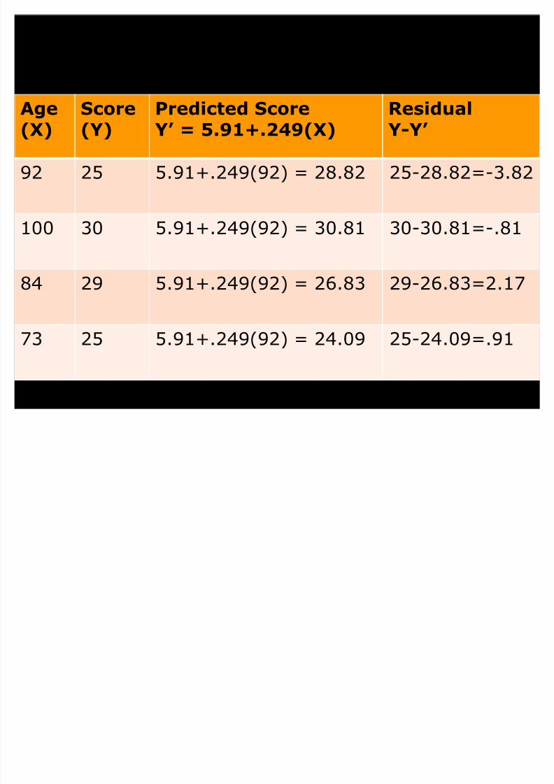
Age(X)
Score(Y)
Predicted ScoreY¶ = 5.91+.249(X)
ResidualY-Y¶
92 25 5.91+.249(92) = 28.82 25-28.82=-3.82
100 30 5.91+.249(92) = 30.81 30-30.81=-.81
84 29 5.91+.249(92) = 26.83 29-26.83=2.17
73 25 5.91+.249(92) = 24.09 25-24.09=.91
8/6/2019 Lecture13 Regression
http://slidepdf.com/reader/full/lecture13-regression 50/54
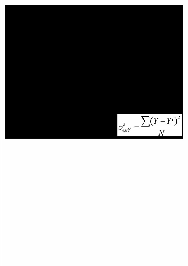
Unexplained variance
� If we went through each of our 100data points, we could calculate theresidual± the value of Y we actually
got minus the value of Y wepredicted from the equation
± The sum of those squared deviations iseverything we didn¶t explain
± The average squared deviations is thevariance of the estimate
W estY
2 !Y dY
2
§ N

8/6/2019 Lecture13 Regression
http://slidepdf.com/reader/full/lecture13-regression 51/54
Explained variance
� The total variance is the variance of Y
� The unexplained variance is theaverage squared deviation score
� Total variance = explained variance +unexplained variance ± So all that¶s left is what we explained by
the regression line ± Explained variance = total variance -
unexplained

8/6/2019 Lecture13 Regression
http://slidepdf.com/reader/full/lecture13-regression 52/54
Coefficient of determination
� We know from our example that thecorrelation between age & test scorewas .72
±We can compute the coefficient of determination by squaring it
± r2 = .722 = .52
� Age accounts for 52% of thevariance in test scores
8/6/2019 Lecture13 Regression
http://slidepdf.com/reader/full/lecture13-regression 53/54
Coefficient of non-determination
� This is simply the reverse²the amount of variance in Y that X does not account for ± An estimate of how much the points don¶t fall
on the line� It is the (unexplained variance)/(total
variance) or (1-r2) ± So 1- .722 = 1 - .52 = .48
�
48% of the variance in test scores is not accounted for by age ± We cannot account for 48% of the variance in
test scores

8/6/2019 Lecture13 Regression
http://slidepdf.com/reader/full/lecture13-regression 54/54
� Next time:
More regression & quizreview
� Happy Spring!
Top Related