


Languages
Pages
Legal

Abdelkader BENHARI
Optimization methods
Introduction and Basic Concepts of optimization problems,Optimization using calculus, Kuhn-Tucker Conditions; Linear Programming - Graphical method,
Simplex method, Revised simplex method, Sensitivity analysis, Examples of transportation, assignment,Dynamic Programming - Introduction, Sequential optimization, computational procedure, curse of dimensionality, Applications in water resources and structural
engineering; Other topics in Optimization - Piecewise linear approximation, Multi objective optimization, Multi level optimization

i
Contents
Introduction and Basic Concepts 1
Historical Development and Model Building 1
Optimization Problem and Model Formulation 6
Classification of Optimization Problems 16
Classical and Advanced Techniques for Optimization 23
Optimization using Calculus-Stationary Points 27
Stationary points: Functions of Single and Two Variables 27
Convexity and Concavity of Functions of One and Two Variables 40
Optimization using Calculus - Unconstrained Optimization 48
Optimization of Functions of Multiple Variables: Unconstrained Optimization 48
Optimization using Calculus – Kuhn-Tucker Conditions 57
Linear Programming- Preliminaries 63
Linear Programming- Graphical Method 70
Linear Programming- Simplex Method-I 76
Linear Programming- Simplex Method – II 87
Revised Simplex Method, Duality and Sensitivity analysis 95
Linear Programming - Other Algorithms for Solving Linear Programming Problems 106
113 Linear Programming Applications – Software
MATLAB Toolbox for Linear Programming 113
Linear Programming Applications – Transportation Problem 116
Transportation Problem 116
Linear Programming -Assignment Problem 125
Linear Programming Applications – Structural & Water Resources Problems 134
Dynamic Programming – Introduction 144
Dynamic Programming – Recursive Equations 150
Computational Procedure in Dynamic Programming 154
Dynamic Programming – Other Topics 158
A.BENHARI

ii
Dynamic Programming Applications – Design of Continuous Beam 161
Dynamic Programming Applications – Optimum Geometric Layout of Truss 163
Optimization Methods: Dynamic Programming Applications – Water Allocation 165
Water Allocation as a Sequential Process – Recursive Equations 165
Water Allocation as a Sequential Process – Numerical Example 170
Dynamic Programming Applications – Capacity Expansion 177
Dynamic Programming Applications – Reservoir Operation 189
Integer Programming – Integer Linear Programming 197
Integer Programming – Mixed Integer Programming 204
Integer Programming – Examples 207
Advanced Topics in Optimization 215
Piecewise linear approximation of a nonlinear function 215
Advanced Topics in Optimization - Multi-objective Optimization 222
Advanced Topics in Optimization - Multilevel Optimization 230
Advanced Topics in Optimization - Direct and Indirect Search Methods 233
Advanced Topics in Optimization - Evolutionary Algorithms for Optimization 239
Advanced Topics in Optimization - Applications in Civil Engineering 246
References 249
A.BENHARI

Optimization Methods: Introduction and Basic Concepts
Historical Development and Model Building
Introduction
In this lecture, historical development of optimization methods is glanced through. Apart
from the major developments, some recently developed novel approaches, such as, goal
programming for multi-objective optimization, simulated annealing, genetic algorithms, and
neural network methods are briefly mentioned tracing their origin. Engineering applications
of optimization with different modeling approaches are scanned through from which one
would get a broad picture of the multitude applications of optimization techniques.
Historical Development
The existence of optimization methods can be traced to the days of Newton, Lagrange, and
Cauchy. The development of differential calculus methods for optimization was possible
because of the contributions of Newton and Leibnitz to calculus. The foundations of calculus
of variations, which deals with the minimization of functions, were laid by Bernoulli, Euler,
Lagrange, and Weistrass. The method of optimization for constrained problems, which
involve the addition of unknown multipliers, became known by the name of its inventor,
Lagrange. Cauchy made the first application of the steepest descent method to solve
unconstrained optimization problems. By the middle of the twentieth century, the high-speed
digital computers made implementation of the complex optimization procedures possible and
stimulated further research on newer methods. Spectacular advances followed, producing a
massive literature on optimization techniques. This advancement also resulted in the
emergence of several well defined new areas in optimization theory.
Some of the major developments in the area of numerical methods of unconstrained
optimization are outlined here with a few milestones.
• Development of the simplex method by Dantzig in 1947 for linear programming
problems
• The enunciation of the principle of optimality in 1957 by Bellman for dynamic
programming problems,
A.BENHARI 1A.BENHARI 1A.BENHARI 1A.BENHARI 1
Optimization Methods: Introduction and Basic Concepts
• Work by Kuhn and Tucker in 1951 on the necessary and sufficient conditions for the
optimal solution of programming problems laid the foundation for later research in
non-linear programming.
• The contributions of Zoutendijk and Rosen to nonlinear programming during the early
1960s have been very significant.
• Work of Carroll and Fiacco and McCormick facilitated many difficult problems to be
solved by using the well-known techniques of unconstrained optimization.
• Geometric programming was developed in the 1960s by Duffin, Zener, and Peterson.
• Gomory did pioneering work in integer programming, one of the most exciting and
rapidly developing areas of optimization. The reason for this is that most real world
applications fall under this category of problems.
• Dantzig and Charnes and Cooper developed stochastic programming techniques and
solved problems by assuming design parameters to be independent and normally
distributed.
The necessity to optimize more than one objective or goal while satisfying the physical
limitations led to the development of multi-objective programming methods. Goal
programming is a well-known technique for solving specific types of multi-objective
optimization problems. The goal programming was originally proposed for linear problems
by Charnes and Cooper in 1961. The foundation of game theory was laid by von Neumann in
1928 and since then the technique has been applied to solve several mathematical, economic
and military problems. Only during the last few years has game theory been applied to solve
engineering problems.
Simulated annealing, genetic algorithms, and neural network methods represent a new class
of mathematical programming techniques that have come into prominence during the last
decade. Simulated annealing is analogous to the physical process of annealing of metals and
glass. The genetic algorithms are search techniques based on the mechanics of natural
selection and natural genetics. Neural network methods are based on solving the problem
using the computing power of a network of interconnected ‘neuron’ processors.
A.BENHARI 2A.BENHARI 2A.BENHARI 2A.BENHARI 2
Optimization Methods: Introduction and Basic Concepts
Engineering applications of optimization
To indicate the widespread scope of the subject, some typical applications in different
engineering disciplines are given below.
• Design of civil engineering structures such as frames, foundations, bridges, towers,
chimneys and dams for minimum cost.
• Design of minimum weight structures for earth quake, wind and other types of
random loading.
• Optimal plastic design of frame structures (e.g., to determine the ultimate moment
capacity for minimum weight of the frame).
• Design of water resources systems for obtaining maximum benefit.
• Design of optimum pipeline networks for process industry.
• Design of aircraft and aerospace structure for minimum weight
• Finding the optimal trajectories of space vehicles.
• Optimum design of linkages, cams, gears, machine tools, and other mechanical
components.
• Selection of machining conditions in metal-cutting processes for minimizing the
product cost.
• Design of material handling equipment such as conveyors, trucks and cranes for
minimizing cost.
• Design of pumps, turbines and heat transfer equipment for maximum efficiency.
• Optimum design of electrical machinery such as motors, generators and transformers.
• Optimum design of electrical networks.
• Optimum design of control systems.
• Optimum design of chemical processing equipments and plants.
• Selection of a site for an industry.
• Planning of maintenance and replacement of equipment to reduce operating costs.
• Inventory control.
• Allocation of resources or services among several activities to maximize the benefit.
• Controlling the waiting and idle times in production lines to reduce the cost of
production.
• Planning the best strategy to obtain maximum profit in the presence of a competitor.
A.BENHARI 3A.BENHARI 3A.BENHARI 3A.BENHARI 3

Optimization Methods: Introduction and Basic Concepts
• Designing the shortest route to be taken by a salesperson to visit various cities in a
single tour.
• Optimal production planning, controlling and scheduling.
• Analysis of statistical data and building empirical models to obtain the most accurate
representation of the statistical phenomenon.
However, the list is incomplete.
Art of Modeling: Model Building
Development of an optimization model can be divided into five major phases.
• Data collection
• Problem definition and formulation
• Model development
• Model validation and evaluation of performance
• Model application and interpretation
Data collection may be time consuming but is the fundamental basis of the model-building
process. The availability and accuracy of data can have considerable effect on the accuracy of
the model and on the ability to evaluate the model.
The problem definition and formulation includes the steps: identification of the decision
variables; formulation of the model objective(s) and the formulation of the model constraints.
In performing these steps the following are to be considered.
• Identify the important elements that the problem consists of.
• Determine the number of independent variables, the number of equations required to
describe the system, and the number of unknown parameters.
• Evaluate the structure and complexity of the model
• Select the degree of accuracy required of the model
Model development includes the mathematical description, parameter estimation, input
development, and software development. The model development phase is an iterative
process that may require returning to the model definition and formulation phase.
The model validation and evaluation phase is checking the performance of the model as a
whole. Model validation consists of validation of the assumptions and parameters of the
A.BENHARI 4A.BENHARI 4A.BENHARI 4A.BENHARI 4

Optimization Methods: Introduction and Basic Concepts
model. The performance of the model is to be evaluated using standard performance
measures such as Root mean squared error and R2 value. A sensitivity analysis should be
performed to test the model inputs and parameters. This phase also is an iterative process and
may require returning to the model definition and formulation phase. One important aspect of
this process is that in most cases data used in the formulation process should be different
from that used in validation. Another point to keep in mind is that no single validation
process is appropriate for all models.
Model application and implementation include the use of the model in the particular area
of the solution and the translation of the results into operating instructions issued in
understandable form to the individuals who will administer the recommended system.
Different modeling techniques are developed to meet the requirements of different types of
optimization problems. Major categories of modeling approaches are: classical optimization
techniques, linear programming, nonlinear programming, geometric programming, dynamic
programming, integer programming, stochastic programming, evolutionary algorithms, etc.
These modeling approaches will be discussed in subsequent modules of this course.
A.BENHARI 5A.BENHARI 5A.BENHARI 5A.BENHARI 5
Optimization Methods: Introduction and Basic concepts
Optimization Problem and Model Formulation
Introduction
In the previous lecture we studied the evolution of optimization methods and their
engineering applications. A brief introduction was also given to the art of modeling. In this
lecture we will study the Optimization problem, its various components and its formulation as
a mathematical programming problem.
Basic components of an optimization problem:
An objective function expresses the main aim of the model which is either to be minimized
or maximized. For example, in a manufacturing process, the aim may be to maximize the
profit or minimize the cost. In comparing the data prescribed by a user-defined model with the
observed data, the aim is minimizing the total deviation of the predictions based on the model
from the observed data. In designing a bridge pier, the goal is to maximize the strength and
minimize size.
A set of unknowns or variables control the value of the objective function. In the
manufacturing problem, the variables may include the amounts of different resources used or
the time spent on each activity. In fitting-the-data problem, the unknowns are the parameters
of the model. In the pier design problem, the variables are the shape and dimensions of the
pier.
A set of constraints are those which allow the unknowns to take on certain values but
exclude others. In the manufacturing problem, one cannot spend negative amount of time on
any activity, so one constraint is that the "time" variables are to be non-negative. In the pier
design problem, one would probably want to limit the breadth of the base and to constrain its
size.
The optimization problem is then to find values of the variables that minimize or maximize
the objective function while satisfying the constraints.
Objective Function
As already stated, the objective function is the mathematical function one wants to maximize
or minimize, subject to certain constraints. Many optimization problems have a single
A.BENHARI 6A.BENHARI 6A.BENHARI 6A.BENHARI 6

Optimization Methods: Introduction and Basic concepts
objective function. (When they don't they can often be reformulated so that they do) The two
exceptions are:
• No objective function. In some cases (for example, design of integrated circuit
layouts), the goal is to find a set of variables that satisfies the constraints of the model.
The user does not particularly want to optimize anything and so there is no reason to
define an objective function. This type of problems is usually called a feasibility
problem.
• Multiple objective functions. In some cases, the user may like to optimize a number of
different objectives concurrently. For instance, in the optimal design of panel of a
door or window, it would be good to minimize weight and maximize strength
simultaneously. Usually, the different objectives are not compatible; the variables that
optimize one objective may be far from optimal for the others. In practice, problems
with multiple objectives are reformulated as single-objective problems by either
forming a weighted combination of the different objectives or by treating some of the
objectives as constraints.
Statement of an optimization problem
An optimization or a mathematical programming problem can be stated as follows:
To find X = which minimizes f(X) (1.1)
⎟⎟⎟⎟⎟⎟
⎠
⎞
⎜⎜⎜⎜⎜⎜
⎝
⎛
nx
xx
.
.2
1
Subject to the constraints
gi(X) 0≤ , i = 1, 2, …., m
lj(X) 0= , j = 1, 2, …., p
where X is an n-dimensional vector called the design vector, f(X) is called the objective
function, and gi(X) and lj(X) are known as inequality and equality constraints, respectively.
The number of variables n and the number of constraints m and/or p need not be related in
any way. This type problem is called a constrained optimization problem.
A.BENHARI 7A.BENHARI 7A.BENHARI 7
Optimization Methods: Introduction and Basic concepts
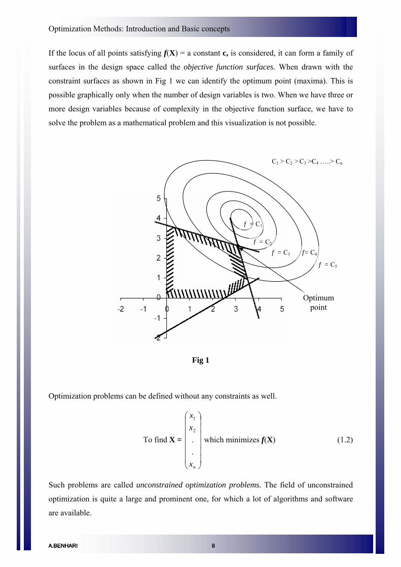
If the locus of all points satisfying f(X) = a constant c, is considered, it can form a family of
surfaces in the design space called the objective function surfaces. When drawn with the
constraint surfaces as shown in Fig 1 we can identify the optimum point (maxima). This is
possible graphically only when the number of design variables is two. When we have three or
more design variables because of complexity in the objective function surface, we have to
solve the problem as a mathematical problem and this visualization is not possible.
.
Optimum point
f = C3
f = C2
f= C4
f = C5
C1 > C2 > C3 >C4 …..> Cn
f = C1
Fig 1
Optimization problems can be defined without any constraints as well.
To find X = which minimizes f(X) (1.2)
⎟⎟⎟⎟⎟⎟
⎠
⎞
⎜⎜⎜⎜⎜⎜
⎝
⎛
nx
xx
.
.2
1
Such problems are called unconstrained optimization problems. The field of unconstrained
optimization is quite a large and prominent one, for which a lot of algorithms and software
are available.
A.BENHARI 8A.BENHARI 8A.BENHARI 8

Optimization Methods: Introduction and Basic concepts
Variables These are essential. If there are no variables, we cannot define the objective function and the
problem constraints. In many practical problems, one cannot choose the design variable
arbitrarily. They have to satisfy certain specified functional and other requirements.
Constraints
Constraints are not essential. It's been argued that almost all problems really do have
constraints. For example, any variable denoting the "number of objects" in a system can only
be useful if it is less than the number of elementary particles in the known universe! In
practice though, answers that make good sense in terms of the underlying physical or
economic criteria can often be obtained without putting constraints on the variables.
Design constraints are restrictions that must be satisfied to produce an acceptable design.
Constraints can be broadly classified as:
1) Behavioral or Functional constraints: These represent limitations on the behavior
performance of the system.
2) Geometric or Side constraints: These represent physical limitations on design
variables such as availability, fabricability, and transportability.
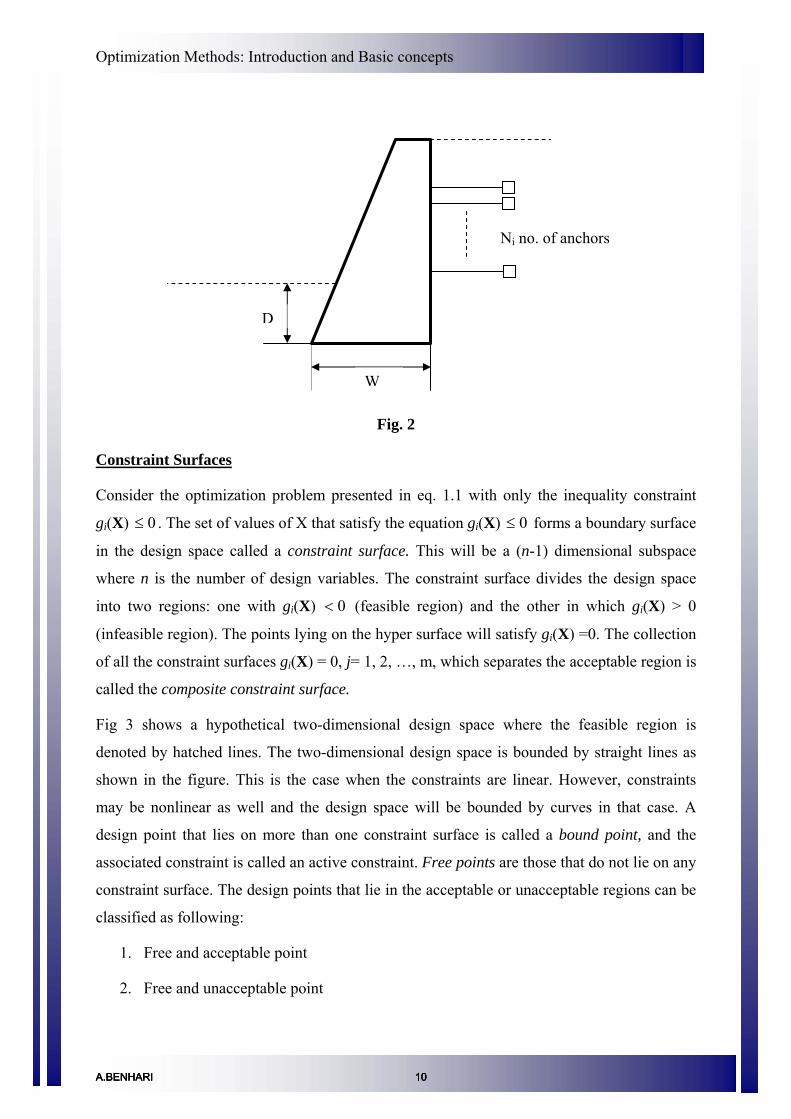
For example, for the retaining wall design shown in the Fig 2, the base width W cannot be
taken smaller than a certain value due to stability requirements. The depth D below the
ground level depends on the soil pressure coefficients Ka and Kp. Since these constraints
depend on the performance of the retaining wall they are called behavioral constraints. The
number of anchors provided along a cross section Ni cannot be any real number but has to be
a whole number. Similarly thickness of reinforcement used is controlled by supplies from the
manufacturer. Hence this is a side constraint.
A.BENHARI 9A.BENHARI 9A.BENHARI 9
Optimization Methods: Introduction and Basic concepts
D
Ni no. of anchors
W
Fig. 2
Constraint Surfaces
Consider the optimization problem presented in eq. 1.1 with only the inequality constraint
gi(X) . The set of values of X that satisfy the equation g0≤ i(X) 0≤ forms a boundary surface
in the design space called a constraint surface. This will be a (n-1) dimensional subspace
where n is the number of design variables. The constraint surface divides the design space
into two regions: one with gi(X) (feasible region) and the other in which g0< i(X) > 0
(infeasible region). The points lying on the hyper surface will satisfy gi(X) =0. The collection
of all the constraint surfaces gi(X) = 0, j= 1, 2, …, m, which separates the acceptable region is
called the composite constraint surface.
Fig 3 shows a hypothetical two-dimensional design space where the feasible region is
denoted by hatched lines. The two-dimensional design space is bounded by straight lines as
shown in the figure. This is the case when the constraints are linear. However, constraints
may be nonlinear as well and the design space will be bounded by curves in that case. A
design point that lies on more than one constraint surface is called a bound point, and the
associated constraint is called an active constraint. Free points are those that do not lie on any
constraint surface. The design points that lie in the acceptable or unacceptable regions can be
classified as following:
1. Free and acceptable point
2. Free and unacceptable point
A.BENHARI 10A.BENHARI 10A.BENHARI 10

Optimization Methods: Introduction and Basic concepts
3. Bound and acceptable point
4. Bound and unacceptable point.
Examples of each case are shown in Fig. 3.
Fig. 3
Bound unacceptable
point.
Behavior constraint
g2 ≤ 0
.
Infeasible region
Feasible region
Behavior constraint
g1 ≤0
Side constraint
g3 ≥ 0
Bound acceptable point.
.
Free acceptable point Free unacceptable
point
Formulation of design problems as mathematical programming problems
In mathematics, the term optimization, or mathematical programming, refers to the study
of problems in which one seeks to minimize or maximize a real function by systematically
choosing the values of real or integer variables from within an allowed set. This problem can
be represented in the following way
Given: a function f : A R from some set A to the real numbers
Sought: an element x0 in A such that f(x0) ≤ f(x) for all x in A ("minimization") or such that
f(x0) ≥ f(x) for all x in A ("maximization").
Such a formulation is called an optimization problem or a mathematical programming
problem (a term not directly related to computer programming, but still in use for example,
A.BENHARI 11A.BENHARI 11A.BENHARI 11

Optimization Methods: Introduction and Basic concepts
in linear programming – (see module 3)). Many real-world and theoretical problems may be
modeled in this general framework.
Typically, A is some subset of the Euclidean space Rn, often specified by a set of constraints,
equalities or inequalities that the members of A have to satisfy. The elements of A are called
candidate solutions or feasible solutions. The function f is called an objective function, or cost
function. A feasible solution that minimizes (or maximizes, if that is the goal) the objective
function is called an optimal solution. The domain A of f is called the search space.
Generally, when the feasible region or the objective function of the problem does not present
convexity (refer module 2), there may be several local minima and maxima, where a local
minimum x* is defined as a point for which there exists some δ > 0 so that for all x such that
;
and
that is to say, on some region around x* all the function values are greater than or equal to the
value at that point. Local maxima are defined similarly.
A large number of algorithms proposed for solving non-convex problems – including the
majority of commercially available solvers – are not capable of making a distinction between
local optimal solutions and rigorous optimal solutions, and will treat the former as the actual
solutions to the original problem. The branch of applied mathematics and numerical analysis
that is concerned with the development of deterministic algorithms that are capable of
guaranteeing convergence in finite time to the actual optimal solution of a non-convex
problem is called global optimization.
Problem formulation
Problem formulation is normally the most difficult part of the process. It is the selection of
design variables, constraints, objective function(s), and models of the discipline/design.
Selection of design variables
A design variable, that takes a numeric or binary value, is controllable from the point of view
of the designer. For instance, the thickness of a structural member can be considered a design
variable. Design variables can be continuous (such as the length of a cantilever beam),
A.BENHARI 12A.BENHARI 12A.BENHARI 12

Optimization Methods: Introduction and Basic concepts
discrete (such as the number of reinforcement bars used in a beam), or Boolean. Design
problems with continuous variables are normally solved more easily.
Design variables are often bounded, that is, they have maximum and minimum values.
Depending on the adopted method, these bounds can be treated as constraints or separately.
Selection of constraints
A constraint is a condition that must be satisfied to render the design to be feasible. An
example of a constraint in beam design is that the resistance offered by the beam at points of
loading must be equal to or greater than the weight of structural member and the load
supported. In addition to physical laws, constraints can reflect resource limitations, user
requirements, or bounds on the validity of the analysis models. Constraints can be used
explicitly by the solution algorithm or can be incorporated into the objective, by using
Lagrange multipliers.
Objectives
An objective is a numerical value that is to be maximized or minimized. For example, a
designer may wish to maximize profit or minimize weight. Many solution methods work only
with single objectives. When using these methods, the designer normally weights the various
objectives and sums them to form a single objective. Other methods allow multi-objective
optimization (module 8), such as the calculation of a Pareto front.
Models
The designer has to also choose models to relate the constraints and the objectives to the
design variables. These models are dependent on the discipline involved. They may be
empirical models, such as a regression analysis of aircraft prices, theoretical models, such as
from computational fluid dynamics, or reduced-order models of either of these. In choosing
the models the designer must trade-off fidelity with the time required for analysis.
The multidisciplinary nature of most design problems complicates model choice and
implementation. Often several iterations are necessary between the disciplines’ analyses in
order to find the values of the objectives and constraints. As an example, the aerodynamic
loads on a bridge affect the structural deformation of the supporting structure. The structural
deformation in turn changes the shape of the bridge and hence the aerodynamic loads. Thus,
it can be considered as a cyclic mechanism. Therefore, in analyzing a bridge, the
A.BENHARI 13A.BENHARI 13A.BENHARI 13

Optimization Methods: Introduction and Basic concepts
aerodynamic and structural analyses must be run a number of times in turn until the loads and
deformation converge.
Representation in standard form
Once the design variables, constraints, objectives, and the relationships between them have
been chosen, the problem can be expressed as shown in equation 1.1
Maximization problems can be converted to minimization problems by multiplying the
objective by -1. Constraints can be reversed in a similar manner. Equality constraints can be
replaced by two inequality constraints.
Problem solution
The problem is normally solved choosing the appropriate techniques from those available in
the field of optimization. These include gradient-based algorithms, population-based
algorithms, or others. Very simple problems can sometimes be expressed linearly; in that case
the techniques of linear programming are applicable.
Gradient-based methods
• Newton's method
• Steepest descent
• Conjugate gradient
• Sequential quadratic programming
Population-based methods
• Genetic algorithms
• Particle swarm optimization
Other methods
• Random search
• Grid search
• Simulated annealing
Most of these techniques require large number of evaluations of the objectives and the
constraints. The disciplinary models are often very complex and can take significant amount
of time for a single evaluation. The solution can therefore be extremely time-consuming.
A.BENHARI 14A.BENHARI 14A.BENHARI 14
Optimization Methods: Introduction and Basic concepts
Many of the optimization techniques are adaptable to parallel computing. Much of the current
research is focused on methods of decreasing the computation time.
The following steps summarize the general procedure used to formulate and solve
optimization problems. Some problems may not require that the engineer follow the steps in
the exact order, but each of the steps should be considered in the process.
1) Analyze the process itself to identify the process variables and specific characteristics
of interest, i.e., make a list of all the variables.
2) Determine the criterion for optimization and specify the objective function in terms of
the above variables together with coefficients.
3) Develop via mathematical expressions a valid process model that relates the input-
output variables of the process and associated coefficients. Include both equality and
inequality constraints. Use well known physical principles such as mass balances,
energy balance, empirical relations, implicit concepts and external restrictions.
Identify the independent and dependent variables to get the number of degrees of
freedom.
4) If the problem formulation is too large in scope:
break it up into manageable parts, or
simplify the objective function and the model
5) Apply a suitable optimization technique for mathematical statement of the problem.
6) Examine the sensitivity of the result, to changes in the values of the parameters in the
problem and the assumptions.
A.BENHARI 15A.BENHARI 15A.BENHARI 15
Optimization Methods: Introduction and Basic Concepts
Classification of Optimization Problems
Introduction
In the previous lecture we studied the basics of an optimization problem and its formulation
as a mathematical programming problem. In this lecture we look at the various criteria for
classification of optimization problems.
Optimization problems can be classified based on the type of constraints, nature of design
variables, physical structure of the problem, nature of the equations involved, deterministic
nature of the variables, permissible value of the design variables, separability of the functions
and number of objective functions. These classifications are briefly discussed below.
Classification based on existence of constraints.
Under this category optimizations problems can be classified into two groups as follows:
Constrained optimization problems: which are subject to one or more constraints.
Unconstrained optimization problems: in which no constraints exist.
Classification based on the nature of the design variables.
There are two broad categories in this classification.
(i) In the first category the objective is to find a set of design parameters that makes a
prescribed function of these parameters minimum or maximum subject to certain constraints.
For example to find the minimum weight design of a strip footing with two loads shown in
Fig 1 (a) subject to a limitation on the maximum settlement of the structure can be stated as
follows.
Find X = which minimizes ⎭⎬⎫
⎩⎨⎧
db
f(X) = h(b,d)
Subject to the constraints (sδ X ) maxδ≤ ; b ≥ 0 ; d ≥ 0
where sδ is the settlement of the footing. Such problems are called parameter or static
optimization problems.
A.BENHARI 16A.BENHARI 16A.BENHARI 16A.BENHARI 16

Optimization Methods: Introduction and Basic Concepts
It may be noted that, for this particular example, the length of the footing (l), the loads P1 and
P2 and the distance between the loads are assumed to be constant and the required
optimization is achieved by varying b and d.
(ii) In the second category of problems, the objective is to find a set of design parameters,
which are all continuous functions of some other parameter that minimizes an objective
function subject to a set of constraints. If the cross sectional dimensions of the rectangular
footings are allowed to vary along its length as shown in Fig 1 (b), the optimization problem
can be stated as :
Find X(t) = which minimizes ⎭⎬⎫
⎩⎨⎧
)()(
tdtb
f(X) = g( b(t), d(t) )
Subject to the constraints
(sδ X(t) ) maxδ≤ 0 ≤ t ≤ l
b(t) 0 0 ≥ ≤ t ≤ l
d(t) 0 0 ≥ ≤ t ≤ l
The length of the footing (l) the loads P1 and P2 , the distance between the loads are assumed
to be constant and the required optimization is achieved by varying b and d along the length l.
Here the design variables are functions of the length parameter t. this type of problem, where
each design variable is a function of one or more parameters, is known as trajectory or
dynamic optimization problem.
l l
P1
P2
d
b
P2
P1
b(t)
d(t)
t
(a) (b)
Fig 1
A.BENHARI 17A.BENHARI 17A.BENHARI 17
Optimization Methods: Introduction and Basic Concepts
Classification based on the physical structure of the problem
Based on the physical structure, optimization problems are classified as optimal control and
non-optimal control problems.
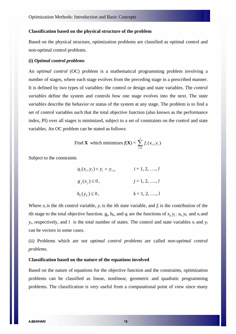
(i) Optimal control problems
An optimal control (OC) problem is a mathematical programming problem involving a
number of stages, where each stage evolves from the preceding stage in a prescribed manner.
It is defined by two types of variables: the control or design and state variables. The control
variables define the system and controls how one stage evolves into the next. The state
variables describe the behavior or status of the system at any stage. The problem is to find a
set of control variables such that the total objective function (also known as the performance
index, PI) over all stages is minimized, subject to a set of constraints on the control and state
variables. An OC problem can be stated as follows:
Find X which minimizes f(X) = ),(1
ii
l
ii yxf∑
=
Subject to the constraints
1),( +=+ iiiii yyyxq i = 1, 2, …., l
0)( ≤jj xg , j = 1, 2, …., l
0)( ≤kk yh , k = 1, 2, …., l
Where xi is the ith control variable, yi is the ith state variable, and fi is the contribution of the
ith stage to the total objective function. gj, hk, and qi are the functions of xj, yj ; xk, yk and xi and
yi, respectively, and l is the total number of states. The control and state variables xi and yi
can be vectors in some cases.
(ii) Problems which are not optimal control problems are called non-optimal control
problems.
Classification based on the nature of the equations involved
Based on the nature of equations for the objective function and the constraints, optimization
problems can be classified as linear, nonlinear, geometric and quadratic programming
problems. The classification is very useful from a computational point of view since many
A.BENHARI 18A.BENHARI 18A.BENHARI 18
Optimization Methods: Introduction and Basic Concepts
predefined special methods are available for effective solution of a particular type of
problem.
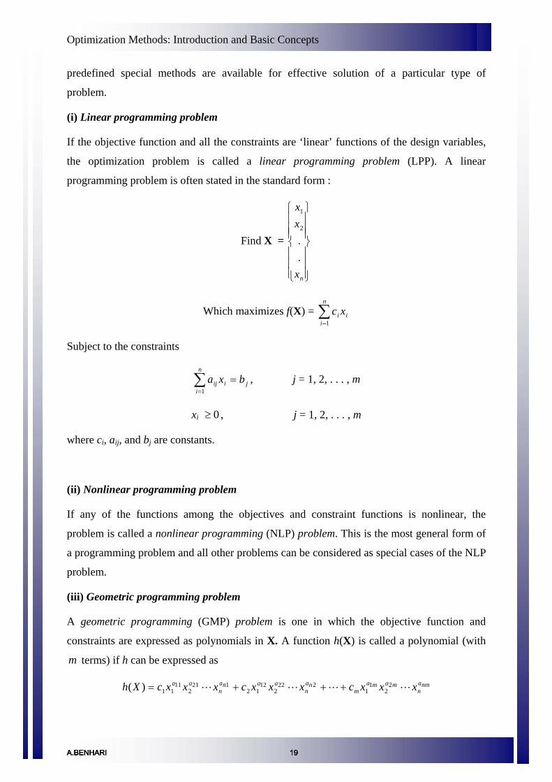
(i) Linear programming problem
If the objective function and all the constraints are ‘linear’ functions of the design variables,
the optimization problem is called a linear programming problem (LPP). A linear
programming problem is often stated in the standard form :
Find X =
⎪⎪⎪
⎭
⎪⎪⎪
⎬
⎫
⎪⎪⎪
⎩
⎪⎪⎪
⎨
⎧
nx
xx
.
.2
1
Which maximizes f(X) = i
n
ii xc∑
=1
Subject to the constraints
ji
n
iij bxa =∑
=1, j = 1, 2, . . . , m
xi , 0≥ j = 1, 2, . . . , m
where ci, aij, and bj are constants.
(ii) Nonlinear programming problem
If any of the functions among the objectives and constraint functions is nonlinear, the
problem is called a nonlinear programming (NLP) problem. This is the most general form of
a programming problem and all other problems can be considered as special cases of the NLP
problem.
(iii) Geometric programming problem
A geometric programming (GMP) problem is one in which the objective function and
constraints are expressed as polynomials in X. A function h(X) is called a polynomial (with
terms) if h can be expressed as m
nman
mamam
nan
aanan
aa xxxcxxxcxxxcXh LLLL 22
11
2222
1212
1212
1111)( +++=
A.BENHARI 19A.BENHARI 19A.BENHARI 19

Optimization Methods: Introduction and Basic Concepts
where cj ( ) and amj ,,1L= ij ( and ni ,,1L= mj ,,1L= ) are constants with and
.
0≥jc
0≥ix
Thus GMP problems can be posed as follows:
Find X which minimizes
f(X) = c,0
1 1∑= =
⎟⎟⎠
⎞⎜⎜⎝
⎛N
j
n
i
ijaij xc C j > 0, xi > 0
subject to
gk(X) = a,01 1∑= =
>⎟⎟⎠
⎞⎜⎜⎝
⎛kN
j
n
i
ijkqijk xa C jk > 0, xi > 0, k = 1,2,…..,m
where N0 and Nk denote the number of terms in the objective function and in the kth constraint
function, respectively.
(iv) Quadratic programming problem
A quadratic programming problem is the best behaved nonlinear programming problem with
a quadratic objective function and linear constraints and is concave (for maximization
problems). It can be solved by suitably modifying the linear programming techniques. It is
usually formulated as follows:
F(X) = ∑∑∑= ==
++n
i
n
jjiij
n
iii xxQxqc
1 11
Subject to
,1
j
n
iiij bxa =∑
=
j = 1,2,….,m
xi , i = 1,2,….,n 0≥
where c, qi, Qij, aij, and bj are constants.
Classification based on the permissible values of the decision variables
Under this classification, objective functions can be classified as integer and real-valued
programming problems.
A.BENHARI 20A.BENHARI 20A.BENHARI 20

Optimization Methods: Introduction and Basic Concepts
(i) Integer programming problem
If some or all of the design variables of an optimization problem are restricted to take only
integer (or discrete) values, the problem is called an integer programming problem. For
example, the optimization is to find number of articles needed for an operation with least
effort. Thus, minimization of the effort required for the operation being the objective, the
decision variables, i.e. the number of articles used can take only integer values. Other
restrictions on minimum and maximum number of usable resources may be imposed.
(ii) Real-valued programming problem
A real-valued problem is that in which it is sought to minimize or maximize a real function
by systematically choosing the values of real variables from within an allowed set. When the
allowed set contains only real values, it is called a real-valued programming problem.
Classification based on deterministic nature of the variables
Under this classification, optimization problems can be classified as deterministic or
stochastic programming problems.
(i) Deterministic programming problem
In a deterministic system, for a same input, the system will produce the same output always.
In this type of problems all the design variables are deterministic.
(ii) Stochastic programming problem
In this type of an optimization problem, some or all the design variables are expressed
probabilistically (non-deterministic or stochastic). For example estimates of life span of
structures which have probabilistic inputs of the concrete strength and load capacity is a
stochastic programming problem as one can only estimate stochastically the life span of the
structure.
Classification based on separability of the functions
Based on this classification, optimization problems can be classified as separable and non-
separable programming problems based on the separability of the objective and constraint
functions.
(i) Separable programming problems
A.BENHARI 21A.BENHARI 21A.BENHARI 21

Optimization Methods: Introduction and Basic Concepts
In this type of a problem the objective function and the constraints are separable. A function
is said to be separable if it can be expressed as the sum of n single-variable functions,
, i.e. ( ) ( ) ( )nni xfxfxf ,..., 221
( )∑=
=n
iii xfXf
1)(
and separable programming problem can be expressed in standard form as :
Find X which minimizes ( )∑=
=n
iii xfXf
1
)(
subject to
( ) j
n
iiijj bxgXg ≤= ∑
=1)( , j = 1,2,. . . , m
where bj is a constant.
Classification based on the number of objective functions
Under this classification, objective functions can be classified as single-objective and multi-
objective programming problems.
(i) Single-objective programming problem in which there is only a single objective function.
(ii) Multi-objective programming problem
A multiobjective programming problem can be stated as follows:
Find X which minimizes ( ) ( ) ( )XfXfXf k,..., 21
Subject to
gj(X) , j = 1, 2, . . . , m 0≤
where f1, f2, . . . fk denote the objective functions to be minimized simultaneously.
For example in some design problems one might have to minimize the cost and weight of the
structural member for economy and, at the same time, maximize the load carrying capacity
under the given constraints.
A.BENHARI 22A.BENHARI 22A.BENHARI 22

Optimization Methods: Introduction and Basic Concepts
Classical and Advanced Techniques for Optimization
In the previous lecture having understood the various classifications of optimization
problems, let us move on to understand the classical and advanced optimization techniques.
Classical Optimization Techniques
The classical optimization techniques are useful in finding the optimum solution or
unconstrained maxima or minima of continuous and differentiable functions. These are
analytical methods and make use of differential calculus in locating the optimum solution.
The classical methods have limited scope in practical applications as some of them involve
objective functions which are not continuous and/or differentiable. Yet, the study of these
classical techniques of optimization form a basis for developing most of the numerical
techniques that have evolved into advanced techniques more suitable to today’s practical
problems. These methods assume that the function is differentiable twice with respect to the
design variables and that the derivatives are continuous. Three main types of problems can be
handled by the classical optimization techniques, viz., single variable functions, multivariable
functions with no constraints and multivariable functions with both equality and inequality
constraints. For problems with equality constraints the Lagrange multiplier method can be
used. If the problem has inequality constraints, the Kuhn-Tucker conditions can be used to
identify the optimum solution. These methods lead to a set of nonlinear simultaneous
equations that may be difficult to solve. These classical methods of optimization are further
discussed in Module 2.
The other methods of optimization include
• Linear programming: studies the case in which the objective function f is linear and
the set A is specified using only linear equalities and inequalities. (A is the design
variable space)
• Integer programming: studies linear programs in which some or all variables are
constrained to take on integer values.
• Quadratic programming: allows the objective function to have quadratic terms,
while the set A must be specified with linear equalities and inequalities.
A.BENHARI 23A.BENHARI 23A.BENHARI 23A.BENHARI 23

Optimization Methods: Introduction and Basic Concepts
• Nonlinear programming: studies the general case in which the objective function or
the constraints or both contain nonlinear parts.
• Stochastic programming: studies the case in which some of the constraints depend
on random variables.
• Dynamic programming: studies the case in which the optimization strategy is based
on splitting the problem into smaller sub-problems.
• Combinatorial optimization: is concerned with problems where the set of feasible
solutions is discrete or can be reduced to a discrete one.
• Infinite-dimensional optimization: studies the case when the set of feasible solutions
is a subset of an infinite-dimensional space, such as a space of functions.
• Constraint satisfaction: studies the case in which the objective function f is constant
(this is used in artificial intelligence, particularly in automated reasoning).
Most of these techniques will be discussed in subsequent modules.
Advanced Optimization Techniques
• Hill climbing
Hill climbing is a graph search algorithm where the current path is extended with a
successor node which is closer to the solution than the end of the current path.
In simple hill climbing, the first closer node is chosen whereas in steepest ascent hill
climbing all successors are compared and the closest to the solution is chosen. Both
forms fail if there is no closer node. This may happen if there are local maxima in the
search space which are not solutions. Steepest ascent hill climbing is similar to best
first search but the latter tries all possible extensions of the current path in order,
whereas steepest ascent only tries one.
Hill climbing is used widely in artificial intelligence fields, for reaching a goal state
from a starting node. Choice of next node starting node can be varied to give a
number of related algorithms.
A.BENHARI 24A.BENHARI 24A.BENHARI 24

Optimization Methods: Introduction and Basic Concepts
• Simulated annealing
The name and inspiration come from annealing process in metallurgy, a technique
involving heating and controlled cooling of a material to increase the size of its
crystals and reduce their defects. The heat causes the atoms to become unstuck from
their initial positions (a local minimum of the internal energy) and wander randomly
through states of higher energy; the slow cooling gives them more chances of finding
configurations with lower internal energy than the initial one.
In the simulated annealing method, each point of the search space is compared to a
state of some physical system, and the function to be minimized is interpreted as the
internal energy of the system in that state. Therefore the goal is to bring the system,
from an arbitrary initial state, to a state with the minimum possible energy.
• Genetic algorithms
A genetic algorithm (GA) is a search technique used in computer science to find
approximate solutions to optimization and search problems. Specifically it falls into
the category of local search techniques and is therefore generally an incomplete
search. Genetic algorithms are a particular class of evolutionary algorithms that use
techniques inspired by evolutionary biology such as inheritance, mutation, selection,
and crossover (also called recombination).
Genetic algorithms are typically implemented as a computer simulation. in which a
population of abstract representations (called chromosomes) of candidate solutions
(called individuals) to an optimization problem, evolves toward better solutions.
Traditionally, solutions are represented in binary as strings of 0s and 1s, but different
encodings are also possible. The evolution starts from a population of completely
random individuals and occur in generations. In each generation, the fitness of the
whole population is evaluated, multiple individuals are stochastically selected from
the current population (based on their fitness), and modified (mutated or recombined)
to form a new population. The new population is then used in the next iteration of the
algorithm.
A.BENHARI 25A.BENHARI 25A.BENHARI 25

Optimization Methods: Introduction and Basic Concepts
• Ant colony optimization
In the real world, ants (initially) wander randomly, and upon finding food return to
their colony while laying down pheromone trails. If other ants find such a path, they
are likely not to keep traveling at random, but instead follow the trail laid by earlier
ants, returning and reinforcing it, if they eventually find any food.
Over time, however, the pheromone trail starts to evaporate, thus reducing its
attractive strength. The more time it takes for an ant to travel down the path and back
again, the more time the pheromones have to evaporate. A short path, by comparison,
gets marched over faster, and thus the pheromone density remains high as it is laid on
the path as fast as it can evaporate. Pheromone evaporation has also the advantage of
avoiding the convergence to a local optimal solution. If there was no evaporation at
all, the paths chosen by the first ants would tend to be excessively attractive to the
following ones. In that case, the exploration of the solution space would be
constrained.
Thus, when one ant finds a good (short) path from the colony to a food source, other
ants are more likely to follow that path, and such positive feedback eventually leaves
all the ants following a single path. The idea of the ant colony algorithm is to mimic
this behavior with "simulated ants" walking around the search space representing the
problem to be solved.
Ant colony optimization algorithms have been used to produce near-optimal solutions
to the traveling salesman problem. They have an advantage over simulated annealing
and genetic algorithm approaches when the graph may change dynamically. The ant
colony algorithm can be run continuously and can adapt to changes in real time. This
is of interest in network routing and urban transportation systems.
A.BENHARI 26A.BENHARI 26A.BENHARI 26

Optimization Methods: Optimization using Calculus-Stationary Points
Stationary points: Functions of Single and Two Variables
Introduction
In this session, stationary points of a function are defined. The necessary and sufficient
conditions for the relative maximum of a function of single or two variables are also
discussed. The global optimum is also defined in comparison to the relative or local optimum.
Stationary points
For a continuous and differentiable function f(x) a stationary point x* is a point at which the
slope of the function vanishes, i.e. f ’(x) = 0 at x = x*, where x* belongs to its domain of
definition.
minimum inflection point maximum
Fig. 1
A stationary point may be a minimum, maximum or an inflection point (Fig. 1).
Relative and Global Optimum
A function is said to have a relative or local minimum at x = x* if * *( ) ( )f x f x h≤ + for all
sufficiently small positive and negative values of h, i.e. in the near vicinity of the point x*.
Similarly a point x* is called a relative or local maximum if * *( ) ( )f x f x h≥ +
*( ) ( )
for all values
of h sufficiently close to zero. A function is said to have a global or absolute minimum at x =
x* if f x f x≤ for all x in the domain over which f(x) is defined. Similarly, a function is
D Nagesh Kumar, IISc, Bangalore
M2L1
A.BENHARI 27A.BENHARI 27A.BENHARI 27A.BENHARI 27

Optimization Methods: Optimization using Calculus-Stationary Points 2
said to have a global or absolute maximum at x = x* if *( ) ( )f x f x≥ for all x in the domain
over which f(x) is defined.
Figure 2 shows the global and local optimum points.
a b a bx x
f(x) f(x)
..
.. .
.A1
B1
B2
A3
A2 Relative minimum is also global optimum (since only one minimum point is there)
A1, A2, A3 = Relative maxima A2 = Global maximum B1, B2 = Relative minima B1 = Global minimum
Fig. 2
Functions of a single variable
Consider the function f(x) defined for a x b≤ ≤ . To find the value of x* ∈ such that x =
x
[ , ]a b* maximizes f(x) we need to solve a single-variable optimization problem. We have the
following theorems to understand the necessary and sufficient conditions for the relative
maximum of a function of a single variable.
Necessary condition: For a single variable function f(x) defined for x which has a
relative maximum at x = x
[ , ]a b∈* , x* ∈ if the derivative [ , ]a b ) /'( ) (f X df x dx= exists as a finite
number at x = x* then f ‘(x*) = 0. This can be understood from the following.
A.BENHARI 28A.BENHARI 28A.BENHARI 28

Optimization Methods: Optimization using Calculus-Stationary Points
Proof.
Since f ‘(x*) is stated to exist, we have
'
0
( * ) ( *)( *) limh
f x h f xf xh→
+ −= (1)
From our earlier discussion on relative maxima we have ( *) ( * )f x f x h≥ + for . Hence 0h →
( * ) ( *) 0f x h f xh
+ −≥ h < 0 (2)
( * ) ( *) 0f x h f xh
+ −≤ h > 0 (3)
which implies for substantially small negative values of h we have and for
substantially small positive values of h we have
( *) 0f x ≥
( *) 0f x ≤ . In order to satisfy both (2) and
(3), f ( *)x
(
= 0. Hence this gives the necessary condition for a relative maxima at x = x* for
)x . f
It has to be kept in mind that the above theorem holds good for relative minimum as well.
The theorem only considers a domain where the function is continuous and differentiable. It
cannot indicate whether a maxima or minima exists at a point where the derivative fails to
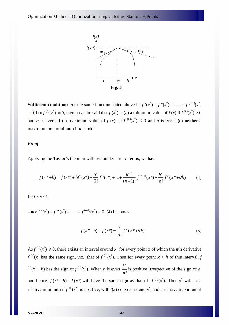
exist. This scenario is shown in Fig 3, where the slopes m1 and m2 at the point of a maxima
are unequal, hence cannot be found as depicted by the theorem by failing for continuity. The
theorem also does not consider if the maxima or minima occurs at the end point of the
interval of definition, owing to the same reason that the function is not continuous, therefore
not differentiable at the boundaries. The theorem does not say whether the function will have
a maximum or minimum at every point where f ‘(x) = 0, since this condition f ‘(x) = 0 is for
stationary points which include inflection points which do not mean a maxima or a minima.
A point of inflection is shown already in Fig.1
A.BENHARI 29A.BENHARI 29A.BENHARI 29
Optimization Methods: Optimization using Calculus-Stationary Points
f(x)
a b x
m2m1f(x*)
x*Fig. 3
Sufficient condition: For the same function stated above let f ’(x*) = f ”(x*) = . . . = f (n-1)(x*)
= 0, but f (n)(x*) 0, then it can be said that f (x≠ *) is (a) a minimum value of f (x) if f (n)(x*) > 0
and n is even; (b) a maximum value of f (x) if f (n)(x*) < 0 and n is even; (c) neither a
maximum or a minimum if n is odd.
Proof
Applying the Taylor’s theorem with remainder after n terms, we have
2 1( 1)( * ) ( *) '( *) ''( *) ... ( *) ( * )
2! ( 1)! !
n nn nh h hf x h f x hf x f x f x f x h
n nθ
−−+ = + + + + + +
− (4)
for 0<θ <1
since f ‘(x*) = f ‘’(x*) = . . . = f (n-1)(x*) = 0, (4) becomes
( * ) ( *) ( * )!
nnhf x h f x f x h
nθ+ − = + (5)
As f (n)(x*) 0, there exists an interval around x≠ * for every point x of which the nth derivative
f (n)(x) has the same sign, viz., that of f (n)(x*). Thus for every point x*+ h of this interval, f
(n)(x*+ h) has the sign of f (n)(x*). When n is even !n
nh
( * ) ( *)
is positive irrespective of the sign of h,
and hence f x h f x+ − will have the same sign as that of f (n)(x*). Thus x* will be a
relative minimum if f (n)(x*) is positive, with f(x) convex around x*, and a relative maximum if
A.BENHARI 30A.BENHARI 30A.BENHARI 30
Optimization Methods: Optimization using Calculus-Stationary Points
f (n)(x*) is negative, with f(x) concave around x*. When n is odd, !n
nh changes sign with the
change in the sign of h and hence the point x* is neither a maximum nor a minimum. In this
case the point x* is called a point of inflection.
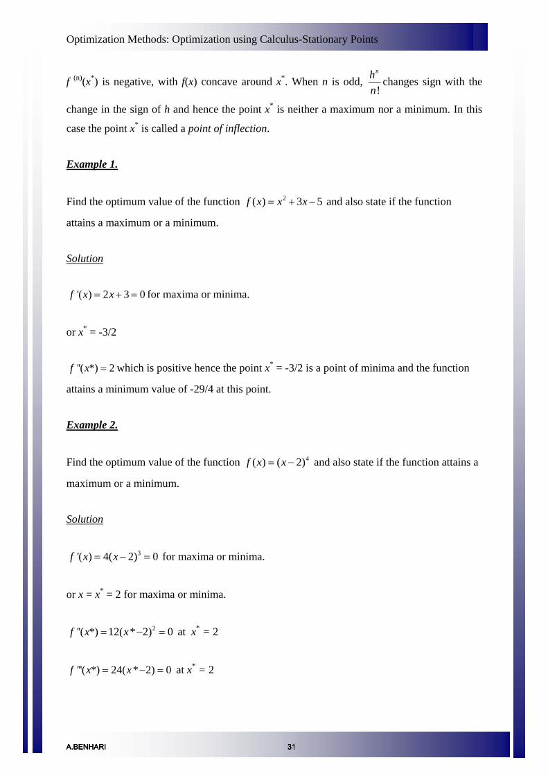
Example 1.
Find the optimum value of the function 2( ) 3 5f x x x= + − and also state if the function
attains a maximum or a minimum.
Solution
'( ) 2 3 0f x x= + = for maxima or minima.
or x* = -3/2
''( *) 2f x = which is positive hence the point x* = -3/2 is a point of minima and the function
attains a minimum value of -29/4 at this point.
Example 2.
Find the optimum value of the function and also state if the function attains a
maximum or a minimum.
4( ) ( 2)f x x= −
Solution
3'( ) 4( 2) 0f x x= − = for maxima or minima.
or x = x* = 2 for maxima or minima.
2''( *) 12( * 2) 0f x x= − = at x* = 2
'''( *) 24( * 2) 0f x x= − = at x* = 2
A.BENHARI 31A.BENHARI 31A.BENHARI 31

Optimization Methods: Optimization using Calculus-Stationary Points
( ) 24* =′′′′ xf at x* = 2
Hence fn(x) is positive and n is even hence the point x = x* = 2 is a point of minimum and the
function attains a minimum value of 0 at this point.
Example 3.
Analyze the function and classify the stationary points as
maxima, minima and points of inflection.
5 4 3( ) 12 45 40 5f x x x x= − + +
Solution
4 3 2
4 3 2
'( ) 60 180 120 0 3 2 0or 0,1,2
f x x x xx x xx
= − + =
=> − + ==
Consider the point x =x* = 0
'' * * 3 * 2 *( ) 240( ) 540( ) 240 0f x x x x= − + =
−
at x * = 0
''' * * 2 *( ) 720( ) 1080 240 240f x x x= − + = at x * = 0
Since the third derivative is non-zero, x = x* = 0 is neither a point of maximum or minimum
but it is a point of inflection.
Consider x = x* = 1
'' * * 3 * 2 *( ) 240( ) 540( ) 240 60f x x x x= − + = at x* = 1
Since the second derivative is negative the point x = x* = 1 is a point of local maxima with a
maximum value of f(x) = 12 – 45 + 40 + 5 = 12
A.BENHARI 32A.BENHARI 32A.BENHARI 32

Optimization Methods: Optimization using Calculus-Stationary Points
Consider x = x* = 2
'' * * 3 * 2 *( ) 240( ) 540( ) 240 240f x x x x= − + = at x* = 2
Since the second derivative is positive, the point x = x* = 2 is a point of local minima with a
minimum value of f(x) = -11
Example 4.
The horse power generated by a Pelton wheel is proportional to u(v-u) where u is the velocity
of the wheel, which is variable and v is the velocity of the jet which is fixed. Show that the
efficiency of the Pelton wheel will be maximum at u = v/2.
Solution
K. ( )
0 K 2K
or 2
0
f u v uf v uu
vu
= −∂
= => − =∂
=
where K is a proportionality constant (assumed positive).
2
2
2
2Kvu
fu
=
∂= −
∂which is negative.
Hence, f is maximum at 2vu =
Functions of two variables
This concept may be easily extended to functions of multiple variables. Functions of two
variables are best illustrated by contour maps, analogous to geographical maps. A contour is a
line representing a constant value of f(x) as shown in Fig.4. From this we can identify
maxima, minima and points of inflection.
A.BENHARI 33A.BENHARI 33A.BENHARI 33

Optimization Methods: Optimization using Calculus-Stationary Points
Necessary conditions
As can be seen in Fig. 4 and 5, perturbations from points of local minima in any direction
result in an increase in the response function f(x), i.e. the slope of the function is zero at this
point of local minima. Similarly, at maxima and points of inflection as the slope is zero, the
first derivatives of the function with respect to the variables are zero.
Which gives us1 2
0; 0f fx x∂ ∂
= =∂ ∂
at the stationary points, i.e., the gradient vector of f(X), x fΔ
at X = X* = [x1, x2] defined as follows, must equal zero:
1
2
( *)0
( *)x
fx
ffx
∂⎡ ⎤Χ⎢ ⎥∂⎢ ⎥Δ = =∂⎢ ⎥
Χ⎢ ⎥∂⎣ ⎦
This is the necessary condition.
x2
x1
Fig. 4
A.BENHARI 34A.BENHARI 34A.BENHARI 34

Optimization Methods: Optimization using Calculus-Stationary Points
Global maxima Relative maxima
Relative minima
Global minima
Fig. 5
Sufficient conditions
Consider the following second order derivatives:
2 2 2
2 21 2 1
; ;2
f f fx x x x
∂ ∂ ∂∂ ∂ ∂ ∂
The Hessian matrix defined by H is made using the above second order derivatives.
A.BENHARI 35A.BENHARI 35A.BENHARI 35

Optimization Methods: Optimization using Calculus-Stationary Points
1 2
2 2
21 1 2
2 2
21 2 2 [ , ]x x
f fx x x
f fx x x
⎛ ⎞∂ ∂⎜ ⎟∂ ∂ ∂⎜ ⎟=⎜ ⎟∂ ∂⎜ ⎟⎜ ⎟∂ ∂ ∂⎝ ⎠
H
a) If H is positive definite then the point X = [x1, x2] is a point of local minima.
b) If H is negative definite then the point X = [x1, x2] is a point of local maxima.
c) If H is neither then the point X = [x1, x2] is neither a point of maxima nor minima.
A square matrix is positive definite if all its eigen values are positive and it is negative
definite if all its eigen values are negative. If some of the eigen values are positive and some
negative then the matrix is neither positive definite or negative definite.
To calculate the eigen valuesλ of a square matrix then the following equation is solved.
0λ− =A I
The above rules give the sufficient conditions for the optimization problem of two variables.
Optimization of multiple variable problems will be discussed in detail in lecture notes 3
(Module 2).
Example 5.
Locate the stationary points of f(X) and classify them as relative maxima, relative minima or
neither based on the rules discussed in the lecture.
f(X) = + 5
A.BENHARI 36A.BENHARI 36A.BENHARI 36

Optimization Methods: Optimization using Calculus-Stationary Points
Solution
From 2
(X) 0fx∂
=∂
, 1 22 2x x= +
From 1
(X) 0fx∂
=∂
22 28 14 3x x 0+ + =
2 2(2 3)(4 1) 0x x+ + =
2 23 / 2 or 1/ 4x x= − = −
so the two stationary points are
X1 = [-1,-3/2]
and
X2 = [3/2,-1/4]
The Hessian of f(X) is
2 2 2 2
12 21 2 1 2 2 1
4 ; 4; 2f f f fxx x x x x x∂ ∂ ∂ ∂
= = = =∂ ∂ ∂ ∂ ∂ ∂
−
A.BENHARI 37A.BENHARI 37A.BENHARI 37

Optimization Methods: Optimization using Calculus-Stationary Points
14 22 4x −⎡ ⎤
= ⎢ ⎥−⎣ ⎦H
14 22 4
xλλ
λ−
=−
I - H
At X1= [-1,-3/2],
4 2( 4)( 4) 4
2 4λ
λ λ λλ
+= = + −
−I - H 0− =
2 16 4 0λ − − =
2λ = 12
1 212 12 λ λ= + = −
Since one eigen value is positive and one negative, X1 is neither a relative maximum nor a
relative minimum.
At X2 = [3/2,-1/4]
6 2( 6)( 4) 4
2 4λ
λ λ λλ
−= = − − −
−I - H 0=
2 10 20 0λ λ− + =
1 25 5 5 5λ λ= + = −
Since both the eigen values are positive, X2 is a local minimum.
Minimum value of f(x) is -0.375.
A.BENHARI 38A.BENHARI 38A.BENHARI 38

Optimization Methods: Optimization using Calculus-Stationary Points
Example 6
The ultimate strength attained by concrete is found to be based on a certain empirical
relationship between the ratios of cement and concrete used. Our objective is to maximize
strength attained by hardened concrete, given by f(X) = , where x2 21 1 2 220 2 6 3 / 2x x x x+ − + − 1
and x2 are variables based on cement and concrete ratios.
Solution
Given f(X) = ; where X = 21 1 2 220 2 6 3 / 2x x x x+ − + − 2 [ ]1 2,x x
The gradient vector 1 1
2
2
( *)2 2 06 3 0( *)
x
fx x
fxf
x
∂⎡ ⎤Χ⎢ ⎥∂ −⎡ ⎤ ⎡ ⎤⎢ ⎥Δ = = =⎢ ⎥ ⎢ ⎥−∂⎢ ⎥ ⎣ ⎦⎣ ⎦Χ⎢ ⎥∂⎣ ⎦
, to determine stationary point X*.
Solving we get X* = [1,2]
2 2 2
2 21 2 1 2
2; 3; 0f f fx x x x∂ ∂ ∂
= − = −∂ ∂ ∂ ∂
=
2 00 3−⎡ ⎤
= ⎢ ⎥−⎣ ⎦H
2 0( 2)( 3)
0 3λ
λ λλ
+= = + +
+I - H 0λ =
Here the values of λ do not depend on X and 1λ = -2, 2λ = -3. Since both the eigen values
are negative, f(X) is concave and the required ratio x1:x2 = 1:2 with a global maximum
strength of f(X) = 27 units.
A.BENHARI 39A.BENHARI 39A.BENHARI 39

Optimization Methods: Optimization using Calculus-Convexity and Concavity
Convexity and Concavity of Functions of One and Two Variables
Introduction
In the previous class we studied about stationary points and the definition of relative and
global optimum. The necessary and sufficient conditions required for a relative optimum in
functions of one variable and its extension to functions of two variables was also studied. In
this lecture, determination of the convexity and concavity of functions is discussed.
The analyst must determine whether the objective functions and constraint equations are
convex or concave. In real-world problems, if the objective function or the constraints are not
convex or concave, the problem is usually mathematically intractable.
Functions of one variable
Convex function
A real-valued function f defined on an interval (or on any convex subset C of some vector
space) is called convex, if for any two points a and b in its domain C and any t in [0,1], we
have
)()1()())1(( bftatfbttaf −+≤−+
Fig. 1
In other words, a function is convex if and only if its epigraph (the set of points lying on or
above the graph) is a convex set. A function is also said to be strictly convex if
A.BENHARI 40A.BENHARI 40A.BENHARI 40A.BENHARI 40

Optimization Methods: Optimization using Calculus-Convexity and Concavity
( (1 ) ) ( ) (1 ) ( )f ta t b tf a t f b+ − < + −
for any t in (0,1) and a line connecting any two points on the function lies completely above
the function. These relationships are illustrated in Fig. 1.
Testing for convexity of a single variable function
A function is convex if its slope is non decreasing or 2 2f / x∂ ∂ ≥ 0. It is strictly convex if its
slope is continually increasing or > 0 throughout the function.
Properties of convex functions
A convex function f, defined on some convex open interval C, is continuous on C and
differentiable at all or at most, countable many points. If C is closed, then f may fail to be
continuous at the end points of C.
A continuous function on an interval C is convex if and only if
( ) ( )2 2
a b f a f bf + +⎛ ⎞ ≤⎜ ⎟⎝ ⎠
for all a and b in C.
A differentiable function of one variable is convex on an interval if and only if its derivative
is monotonically non-decreasing on that interval.
A continuously differentiable function of one variable is convex on an interval if and only if
the function lies above all of its tangents: ( ) ( ) '( )( )f b f a f a b a≥ + − for all a and b in the
interval.
A twice differentiable function of one variable is convex on an interval if and only if its
second derivative is non-negative in that interval; this gives a practical test for convexity. If
its second derivative is positive then it is strictly convex, but the converse does not hold, as
shown by f(x) = x4.
More generally, a continuous, twice differentiable function of several variables is convex on
a convex set if and only if its Hessian matrix is positive semi definite on the interior of the
convex set.
A.BENHARI 41A.BENHARI 41A.BENHARI 41

Optimization Methods: Optimization using Calculus-Convexity and Concavity
If two functions f and g are convex, then so is any weighted combination a f + b g with non-
negative coefficients a and b. Likewise, if f and g are convex, then the function max{f,g} is
convex.
A strictly convex function will have only one minimum which is also the global minimum.
Examples
• The second derivative of x2 is 2; it follows that x2 is a convex function of x.
• The absolute value function |x| is convex, even though it does not have a derivative at
x = 0.
• The function f with domain [0,1] defined by f(0)=f(1)=1, f(x)=0 for 0<x<1 is convex;
it is continuous on the open interval (0,1), but not continuous at 0 and 1.
• Every linear transformation is convex but not strictly convex, since if f is linear, then
f(a + b) = f(a) + f(b). This implies that the identity map (i.e., f(x) = x) is convex but
not strictly convex. The fact holds good if we replace "convex" by "concave".
• An affine function (f (x) = ax + b) is simultaneously convex and concave.
Concave function
A differentiable function f is concave on an interval if its derivative function f ′ is decreasing
on that interval: a concave function has a decreasing slope.
A function that is convex is often synonymously called concave upwards, and a function
that is concave is often synonymously called concave downward.
For a twice-differentiable function f, if the second derivative, f ''(x), is positive (or, if the
acceleration is positive), then the graph is convex (or concave upward); if the second
derivative is negative, then the graph is concave (or concave downward). Points, at which
concavity changes, are called inflection points.
If a convex (i.e., concave upward) function has a "bottom", any point at the bottom is a
minimal extremum. If a concave (i.e., concave downward) function has an "apex", any point
at the apex is a maximal extremum.
A function f(x) is said to be concave on an interval if, for all a and b in that interval,
A.BENHARI 42A.BENHARI 42A.BENHARI 42

Optimization Methods: Optimization using Calculus-Convexity and Concavity
[0,1], ( (1 ) ) ( ) (1 ) ( )t f ta t b tf a t f∀ ∈ + − ≥ + − b
Additionally, f(x) is strictly concave if
[0,1], ( (1 ) ) ( ) (1 ) ( )t f ta t b tf a t f b∀ ∈ + − > + −
These relationships are illustrated in Fig. 2
Fig. 2
Testing for concavity of a single variable function
A function is concave if its slope is non increasing or 2 2/f x∂ ∂ ≤ 0. It is strictly concave if its
slope is continually decreasing or 2 2/f x∂ ∂ <0 throughout the function.
Properties of a concave functions
A continuous function on C is concave if and only if
( ) ( )2 2
a b f a f bf + +⎛ ⎞ ≥⎜ ⎟⎝ ⎠
for any x and y in C.
Equivalently, f(x) is concave on [a, b] if and only if the function −f(x) is convex on every
subinterval of [a, b].
A.BENHARI 43A.BENHARI 43A.BENHARI 43

Optimization Methods: Optimization using Calculus-Convexity and Concavity
If f(x) is twice-differentiable, then f(x) is concave if and only if f ′′(x) is non-positive. If its
second derivative is negative then it is strictly concave, but the opposite is not true, as shown
by f(x) = -x4.
A function is called quasiconcave if and only if there is an x0 such that for all x < x0, f(x) is
non-decreasing while for all x > x0 it is non-increasing. x0 can also be , making the
function non-decreasing (non-increasing) for all
±∞
x. The opposite of quasiconcave is
quasiconvex.
Example 1
Consider the example in lecture notes 1 for a function of two variables. Locate the stationary
points of and find out if the function is convex, concave or
neither at the points of optima based on the testing rules discussed above.
5 4 3( ) 12 45 40 5f x x x x= − + +
Solution 4 3 2
4 3 2
'( ) 60 180 120 0 3 2 0or 0,1,2
f x x x xx x xx
= − + =
=> − + ==
Consider the point x =x* = 0 3 2''( *) 240( *) 540( *) 240 * 0f x x x x= − + =
−
at x * = 0 2'''( *) 720( *) 1080 * 240 240f x x x= − + = at x * = 0
Since the third derivative is non-zero x = x* = 0 is neither a point of maximum or minimum
but it is a point of inflection. Hence the function is neither convex nor concave at this point.
Consider x = x* = 1 3 2''( *) 240( *) 540( *) 240 * 60f x x x x= − + = at x* = 1
Since the second derivative is negative, the point x = x* = 1 is a point of local maxima with a
maximum value of f(x) = 12 – 45 + 40 + 5 = 12. At this point the function is concave since 2 2/f x∂ ∂ < 0.
Consider x = x* = 2 3 2''( *) 240( *) 540( *) 240 * 240f x x x x= − + = at x* = 2
Since the second derivative is positive, the point x = x* = 2 is a point of local minima with a
minimum value of f(x) = -11. At this point the function is convex since 2 2/f x∂ ∂ > 0.
A.BENHARI 44A.BENHARI 44A.BENHARI 44

Optimization Methods: Optimization using Calculus-Convexity and Concavity
Functions of two variables
A function of two variables, f(X) where X is a vector = [x1,x2], is strictly convex if
1 2 1( (1 ) ) ( ) (1 ) ( )f t t tf t fΧ + − Χ < Χ + − Χ2
2
where X1 and X2 are points located by the coordinates given in their respective vectors.
Similarly a two variable function is strictly concave if
1 2 1( (1 ) ) ( ) (1 ) ( )f t t tf t fΧ + − Χ > Χ + − Χ
Contour plot of a convex function is illustrated in Fig. 3
340
Fig. 3
Contour plot of a convex function is shown in Fig. 4
Fig. 4
450
70 x2
120
x1
x2
x1
110
210
305
40
A.BENHARI 45A.BENHARI 45A.BENHARI 45

Optimization Methods: Optimization using Calculus-Convexity and Concavity
To determine convexity or concavity of a function of multiple variables, the eigenvalues of
its Hessian matrix are examined and the following rules apply.
(a) If all eigenvalues of the Hessian are positive the function is strictly convex.
(b) If all eigenvalues of the Hessian are negative the function is strictly concave.
(c) If some eigenvalues are positive and some are negative, or if some are zero, the
function is neither strictly concave nor strictly convex.
Example 2
Consider the example in lecture notes 1 for a function of two variables. Locate the stationary
points of f(X) and find out if the function is convex, concave or neither at the points of
optima based on the rules discussed in this lecture.
f(X) = 3 21 1 2 1 22 / 3 2 5 2 4 2x x x x x x− − + + + 5
Solution
21 1 2
1 2
2
( *)02 2 502 4 4( *)
x
fx x x
ff x xx
∂⎡ ⎤Χ⎢ ⎥∂ ⎡ ⎤− − ⎡ ⎤⎢ ⎥Δ = = =⎢ ⎥ ⎢ ⎥∂⎢ ⎥ − + + ⎣ ⎦⎣ ⎦Χ⎢ ⎥∂⎣ ⎦
Solving the above the two stationary points are
X1 = [-1,-3/2]
and
X2 = [3/2,-1/4]
The Hessian of f(X) is 2 2 2 2
12 21 2 1 2 2 1
4 ; 4; 2f f f fxx x x x x x∂ ∂ ∂ ∂
= = = =∂ ∂ ∂ ∂ ∂ ∂
−
14 22 4x −⎡ ⎤
= ⎢ ⎥−⎣ ⎦H
14 22 4
xλλ
λ−
=−
I - H
At X1
4 2( 4)( 4) 4
2 4λ
λ λ λλ
+= = + −
−I - H 0− =
2 16 4 0λ − − =
A.BENHARI 46A.BENHARI 46A.BENHARI 46

Optimization Methods: Optimization using Calculus-Convexity and Concavity
2λ = 12
1 212 12 λ λ= + = −
Since one eigen value is positive and one negative, X1 is neither a relative maximum nor a
relative minimum. Hence at X1 the function is neither convex nor concave.
At X2 = [3/2,-1/4]
6 2( 6)( 4) 4
2 4λ
λ λ λλ
−= = − − −
−I - H 0=
2 10 20 0λ λ− + =
1 25 5 5 5λ λ= + = −
Since both the eigen values are positive, X2 is a local minimum, and the function is convex at
this point as both the eigen values are positive.
A.BENHARI 47A.BENHARI 47A.BENHARI 47A.BENHARI 47

Optimization Methods: Optimization using Calculus - Unconstrained Optimization
Optimization of Functions of Multiple Variables: Unconstrained Optimization
Introduction
In the previous lectures we learnt how to determine the convexity and concavity of functions
of single and two variables. For functions of single and two variables we also learnt
determining stationary points and examining higher derivatives to check for convexity and
concavity, and tests were recommended to evaluate stationary points as local minima, local
maxima or points of inflection.
In this lecture functions of multiple variables, which are more difficult to be analyzed owing
to the difficulty in graphical representation and tedious calculations involved in mathematical
analysis, will be studied for unconstrained optimization. This is done with the aid of the
gradient vector and the Hessian matrix. Examples are discussed to show the implementation
of the technique.
Unconstrained optimization
If a convex function is to be minimized, the stationary point is the global minimum and
analysis is relatively straightforward as discussed earlier. A similar situation exists for
maximizing a concave variable function. The necessary and sufficient conditions for the
optimization of unconstrained function of several variables are given below.
Necessary condition
In case of multivariable functions a necessary condition for a stationary point of the function
f(X) is that each partial derivative is equal to zero. In other words, each element of the
gradient vector defined below must be equal to zero.
i.e. the gradient vector of f(X), x fΔ at X=X*, defined as follows, must be equal to zero:
1
2
( *)
( *)
( *)
x
n
fxfx
f
fdx
∂⎡ ⎤Χ⎢ ⎥∂⎢ ⎥∂⎢ ⎥
Χ⎢ ⎥∂⎢ ⎥Δ =⎢ ⎥⎢ ⎥⎢ ⎥⎢ ⎥∂
Χ⎢ ⎥∂⎣ ⎦
M
M
= 0
A.BENHARI 48A.BENHARI 48A.BENHARI 48A.BENHARI 48

Optimization Methods: Optimization using Calculus - Unconstrained Optimization
The proof given for the theorem on necessary condition for single variable optimization can
be easily extended to prove the present condition.
Sufficient condition
For a stationary point X* to be an extreme point, the matrix of second partial derivatives
(Hessian matrix) of f(X) evaluated at X* must be:
(i) positive definite when X* is a point of relative minimum, and
(ii) negative definite when X* is a relative maximum point.
Proof (Formulation of the Hessian matrix)
The Taylor’s theorem with reminder after two terms gives us
2
1 1 1 *
1( * ) ( *) ( *)2!
n n n
i i ji i ji i h
df ff h f h h hdx x x j θ= = = Χ=Χ +
∂Χ + = Χ + Χ +
∂ ∂∑ ∑∑
0<θ <1
Since X* is a stationary point, the necessary condition gives
0i
dfdx
= , i = 1,2,…,n
Thus
2
1 1 *
1( * ) ( *)2!
n n
i ji j i j h
ff h f h hx x
θ= = Χ=Χ +
∂Χ + − Χ =
∂ ∂∑∑
For a minimization problem the left hand side of the above expression must be positive.
Since the second partial derivative is continuous in the neighborhood of X* the sign of 2 *i jf x x hθ∂ ∂ ∂ Χ = Χ + is the same as the sign of 2 *i jf x x∂ ∂ ∂ Χ = Χ . And hence
will be a relative minimum, if ( * ) ( *)f h fΧ + − Χ
2
1 1 *
1( * ) ( *)2!
n n
i ji j i j
ff h f h hx x= = Χ=Χ
∂Χ + − Χ =
∂ ∂∑∑
is positive. This can also be written in the matrix form as
X=X*
TQ = h Hh
where
2
X=X**i j
fx x
Χ=Χ
⎡ ⎤∂= ⎢ ⎥
∂ ∂⎢ ⎥⎣ ⎦H
is the matrix of second partial derivatives and is called the Hessian matrix of f(X).
A.BENHARI 49A.BENHARI 49A.BENHARI 49

Optimization Methods: Optimization using Calculus - Unconstrained Optimization
Q will be positive for all h if and only if H is positive definite at X=X*. i.e. the sufficient
condition for X* to be a relative minimum is that the Hessian matrix evaluated at the same
point is positive definite, which completes the proof for the minimization case. In a similar
manner, it can be proved that the Hessian matrix will be negative definite if X* is a point of
relative maximum.
A matrix A will be positive definite if all its eigenvalues are positive. i.e. all values ofλ that
satisfy the equation
0λ− =A I
should be positive. Similarly, the matrix A will be negative definite if its eigenvalues are
negative. When some eigenvalues are positive and some are negative then matrix A is neither
positive definite or negative definite.
When all eigenvalues are negative for all possible values of X, then X* is a global maximum,
and when all eigenvalues are positive for all possible values of X, then X* is a global
minimum.
If some of the eigenvalues of the Hessian at X* are positive and some negative, or if some are
zero, the stationary point, X*, is neither a local maximum nor a local minimum.
Example
Analyze the function and classify the
stationary points as maxima, minima and points of inflection.
2 2 21 2 3 1 2 1 3 1 3( ) 2 2 4 5 2f x x x x x x x x x x= − − − + + + − +
Solution
11 2 3
2 12
3 1
3
( *)2 2 2 4 0
( *) 2 2 02 2 5 0
( *)
x
fx x x xff x xx
x xfx
⎡ ⎤∂Χ⎢ ⎥∂⎢ ⎥ − + + +⎡ ⎤ ⎡ ⎤
⎢ ⎥∂ ⎢ ⎥ ⎢ ⎥Δ = Χ = − + =⎢ ⎥ ⎢ ⎥ ⎢ ⎥∂⎢ ⎥ ⎢ ⎥ ⎢ ⎥− + −⎣ ⎦ ⎣ ⎦⎢ ⎥∂Χ⎢ ⎥
∂⎣ ⎦
Solving these simultaneous equations we get X*=[1/2, 1/2, -2] 2 2 2
2 2 21 2 32 2
1 2 2 1
2; 2; 2
2
f f fx x x
f fx x x x
∂ ∂ ∂= − = − =
∂ ∂ ∂
∂ ∂= =
∂ ∂ ∂ ∂
−
A.BENHARI 50A.BENHARI 50A.BENHARI 50
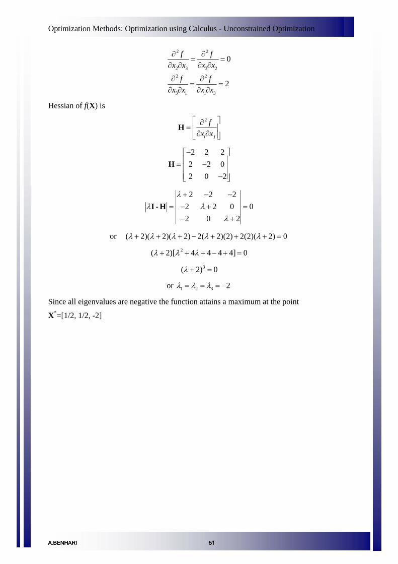
Optimization Methods: Optimization using Calculus - Unconstrained Optimization
2 2
2 3 3 22 2
3 1 1 3
0
2
f fx x x x
f fx x x x
∂ ∂= =
∂ ∂ ∂ ∂
∂ ∂= =
∂ ∂ ∂ ∂
Hessian of f(X) is 2
i j
fx x
⎡ ⎤∂= ⎢ ⎥
∂ ∂⎢ ⎥⎣ ⎦H
2 2 22 2 02 0 2
−⎡ ⎤⎢ ⎥= −⎢ ⎥⎢ ⎥−⎣ ⎦
H
2 2 22 2 02 0 2
λλ λ
λ
+ − −0= − + =
− +I - H
or ( 2)( 2)( 2) 2( 2)(2) 2(2)( 2) 0λ λ λ λ λ+ + + − + + + = 2( 2)[ 4 4 4 4]λ λ λ+ + + − + = 0
0
3( 2)λ + =
or 1 2 3 2λ λ λ= = = −
Since all eigenvalues are negative the function attains a maximum at the point
X*=[1/2, 1/2, -2]
A.BENHARI 51A.BENHARI 51A.BENHARI 51

Optimization Methods: Optimization using Calculus - Equality constraints
Since g(x1*,x2*) = 0 at the minimum point, variations dx1 and dx2 about the point [x1*, x2*]
must be admissible variations, i.e. the point lies on the constraint:
g(x1* + dx1 , x2* + dx2) = 0 (2)
assuming dx1 and dx2 are small the Taylor series expansion of this gives us
1 1 2 2 1 2 1 2 1 1 2 21 2
( * , * ) ( *, *) (x *,x *) (x *,x *) 0g gg x dx x dx g x x dx dxx x∂ ∂
+ + = + +∂ ∂
= (3)
or
1 21 2
0g gdg dx dxx x∂ ∂
= +∂ ∂
=
0
at [x1*,x2*] (4)
which is the condition that must be satisfied for all admissible variations.
Assuming (4)2/g x∂ ∂ ≠ can be rewritten as
12 1
2
/ ( *, *)/
g xdx x x dxg x 2 1∂ ∂
= −∂ ∂
(5)
which indicates that once variation along x1 (d x1) is chosen arbitrarily, the variation along x2
(d x2) is decided automatically to satisfy the condition for the admissible variation.
Substituting equation (5) in (1)we have:
1 2
11
1 2 2 (x *, x *)
/ 0/
g xf fdf dxx g x x
⎛ ⎞∂ ∂∂ ∂= − =⎜ ⎟∂ ∂ ∂ ∂⎝ ⎠
(6)
The equation on the left hand side is called the constrained variation of f. Equation (5) has to
be satisfied for all dx1, hence we have
1 21 2 2 1 (x *, x *)
0f g f gx x x x
⎛ ⎞∂ ∂ ∂ ∂− =⎜ ⎟∂ ∂ ∂ ∂⎝ ⎠
(7)
This gives us the necessary condition to have [x1*, x2*] as an extreme point (maximum or
minimum)
Solution by method of Lagrange multipliers
Continuing with the same specific case of the optimization problem with n = 2 and m = 1 we
define a quantityλ , called the Lagrange multiplier as
1 2
2
2 (x *, x *)
//
f xg x
λ ∂ ∂= −
∂ ∂ (8)
Using this in (6)
A.BENHARI 52A.BENHARI 52A.BENHARI 52
Optimization Methods: Optimization using Calculus - Equality constraints 3
1 21 1 (x *, x *)
0f gx x
λ⎛ ⎞∂ ∂
+ =⎜ ⎟∂ ∂⎝ ⎠ (9)
And (8) written as
1 22 2 (x *, x *)
0f gx x
λ⎛ ⎞∂ ∂
+ =⎜ ⎟∂ ∂⎝ ⎠ (10)
Also, the constraint equation has to be satisfied at the extreme point
1 21 2 ( *, *)
( , ) 0x x
g x x = (11)
Hence equations (9) to (11) represent the necessary conditions for the point [x1*, x2*] to be
an extreme point.
Note that λ could be expressed in terms of 1/g x∂ ∂ as well and 1/g x∂ ∂ has to be non-zero.
Thus, these necessary conditions require that at least one of the partial derivatives of g(x1, x2)
be non-zero at an extreme point.
The conditions given by equations (9) to (11) can also be generated by constructing a
function L, known as the Lagrangian function, as
1 2 1 2 1 2( , , ) ( , ) ( , )L x x f x x g x xλ λ= + (12)
Alternatively, treating L as a function of x1,x2 and λ , the necessary conditions for its
extremum are given by
1 2 1 2 1 21 1 1
1 2 1 2 1 22 2 2
1 2 1 2
( , , ) ( , ) ( , ) 0
( , , ) ( , ) ( , ) 0
( , , ) ( , ) 0
L f gx x x x x xx x xL f gx x x x x xx x xL x x g x x
λ λ
λ λ
λλ
∂ ∂ ∂= + =
∂ ∂ ∂∂ ∂ ∂
= +∂ ∂ ∂∂
= =∂
= (13)
The necessary and sufficient conditions for a general problem are discussed next.
Necessary conditions for a general problem
For a general problem with n variables and m equality constraints the problem is defined as
shown earlier
Maximize (or minimize) f(X), subject to gj(X) = 0, j = 1, 2, … , m
where
1
2
n
xx
x
⎧ ⎫⎪ ⎪⎪ ⎪= ⎨ ⎬⎪ ⎪⎪ ⎪⎩ ⎭
XM
A.BENHARI 53A.BENHARI 53A.BENHARI 53

Optimization Methods: Optimization using Calculus - Equality constraints 4
In this case the Lagrange function, L, will have one Lagrange multiplier jλ for each constraint
as (X)jg
1 2 , 1 2 1 1 2 2( , ,..., , ,..., ) ( ) ( ) ( ) ... ( )n m m mL x x x f g g gλ λ λ λ λ λ= + + + +X X X X
m
(14)
L is now a function of n + m unknowns, 1 2 , 1 2, ,..., , ,...,nx x x λ λ λ , and the necessary conditions
for the problem defined above are given by
1( ) ( ) 0, 1, 2,..., 1, 2,...,
( ) 0, 1, 2,...,
mj
jji i i
jj
gL f i n jx x xL g j m
λ
λ
=
∂∂ ∂= + = = =
∂ ∂ ∂
∂= = =
∂
∑X X
X
m (15)
which represent n + m equations in terms of the n + m unknowns, xi and jλ . The solution to
this set of equations gives us
1
2
**
*n
xx
x
⎧ ⎫⎪ ⎪⎪= ⎨⎪ ⎪⎪ ⎪⎩ ⎭
XM
⎪⎬ and
1
2
**
*
*m
λλ
λ
λ
⎧ ⎫⎪ ⎪⎪ ⎪= ⎨ ⎬⎪ ⎪⎪ ⎪⎩ ⎭
M (16)
The vector X corresponds to the relative constrained minimum of f(X) (subject to the
verification of sufficient conditions).
Sufficient conditions for a general problem
A sufficient condition for f(X) to have a relative minimum at X* is that each root of the
polynomial in ∈ , defined by the following determinant equation be positive.
11 12 1 11 21 1
21 22 2 12 22 2
1 2 1 2
11 12 1
21 22 2
1 2
00 0
0 0
n m
n m
n n nn n n mn
n
n
m m mn
L L L g g gL L L g g g
L L L g g g
g g gg g g
g g g
−∈−∈
−∈=
L L
M O M M O M
L L
L L L
M O M
M O M M M
L L L
(17)
A.BENHARI 54A.BENHARI 54A.BENHARI 54
Optimization Methods: Optimization using Calculus - Equality constraints
where 2
( *, *), for 1, 2,..., 1, 2,...,
( *), where 1, 2,..., and 1, 2,...,
iji j
ppq
q
LL i n jx x
gg p m
x
λ∂= =∂ ∂
∂= =∂
X
X
m
q n
=
=
2
(18)
Similarly, a sufficient condition for f(X) to have a relative maximum at X* is that each root of
the polynomial in ∈ , defined by equation (17) be negative. If equation (17), on solving yields
roots, some of which are positive and others negative, then the point X* is neither a
maximum nor a minimum.
Example
Minimize 2 21 1 2 2 1( ) 3 6 5 7 5f x x x x x= − − − + +X x
Subject to 1 2 5x x+ =
Solution
1 1 2( ) 5 0g x x= + − =X
1 2 , 1 2 1 1 2 2( , ,..., , ,..., ) ( ) ( ) ( ) ... ( )n m m mx x x f g g gλ λ λ λ λ λ= + + + +L X X X X
)
with n = 2 and m = 1
L = 2 21 1 2 2 1 2 1 1 23 6 5 7 5 ( 5x x x x x x x xλ− − − + + + + −
1 2 11
1 2 1
1
6 6 7
1 (7 )6
15 (7 )6
x xx
x x
λ
λ
λ
∂ 0= − − + + =∂
=> + = +
=> = +
L
or 1 23λ =
1 2 12
1 2 1
1 2 2 1
6 10 5 0
13 5 (5 )2
13( ) 2 (5 )2
x xx
x x
x x x
λ
λ
λ
∂= − − + + =
∂
=> + = +
=> + + = +
L
A.BENHARI 55A.BENHARI 55A.BENHARI 55

Optimization Methods: Optimization using Calculus - Equality constraints
21
2x −=
and, 1112
x =
Hence [ ]1 11* , ; * 22 2−⎡ ⎤= =⎢ ⎥⎣ ⎦
X λ 3
11 12 11
21 22 21
11 12
00
L L gL L gg g
−∈⎛ ⎞⎜ ⎟−∈ =⎜ ⎟⎜ ⎟⎝ ⎠
2
11 21 ( )
6Lx
∂= =∂
X*,λ*
L−
2
12 211 2 ( )
6L Lx x∂
= = = −∂ ∂
X*,λ*
L
2
22 22 ( )
10Lx
∂= =∂
X*,λ*
L−
111
1 ( )
112 21
2 ( )
1
1
ggx
gg gx
∂= =∂
∂= = =
∂
X*,λ*
X*,λ*
The determinant becomes
6 6 16 10 1
1 1 0
− −∈ −⎛ ⎞⎜ ⎟ 0− − −∈ =⎜ ⎟⎜ ⎟⎝ ⎠
or ( 6 )[ 1] ( 6)[ 1] 1[ 6 10 ] 0
2− −∈ − − − − + − + +∈ ==>∈= −
Since ∈ is negative, X*, correspond to a maximum. *λ
A.BENHARI 56A.BENHARI 56A.BENHARI 56

Optimization Methods: Optimization using Calculus – Kuhn-Tucker Conditions
Kuhn-Tucker Conditions
Introduction
In the previous lecture the optimization of functions of multiple variables subjected to
equality constraints using the method of constrained variation and the method of Lagrange
multipliers was dealt. In this lecture the Kuhn-Tucker conditions will be discussed with
examples for a point to be a local optimum in case of a function subject to inequality
constraints.
Kuhn-Tucker Conditions
It was previously established that for both an unconstrained optimization problem and an
optimization problem with an equality constraint the first-order conditions are sufficient for a
global optimum when the objective and constraint functions satisfy appropriate
concavity/convexity conditions. The same is true for an optimization problem with inequality
constraints.
The Kuhn-Tucker conditions are both necessary and sufficient if the objective function is
concave and each constraint is linear or each constraint function is concave, i.e. the problems
belong to a class called the convex programming problems.
Consider the following optimization problem:
Minimize f(X) subject to gj(X) ≤ 0 for j = 1,2,…,p ; where X = [x1 x2 . . . xn]
Then the Kuhn-Tucker conditions for X* = [x1* x2
* . . . xn*] to be a local minimum are
10 1, 2,...,
0 1, 2,...,
0 1, 2,...,
0 1, 2,...,
m
jji i
j j
j
j
f g i nx x
g j
g j
m
m
j m
λ
λ
λ
=
∂ ∂+ = =
∂ ∂
= =
≤ =
≥ =
∑ (1)
A.BENHARI 57A.BENHARI 57A.BENHARI 57A.BENHARI 57

Optimization Methods: Optimization using Calculus – Kuhn-Tucker Conditions
In case of minimization problems, if the constraints are of the form gj(X) 0, then ≥ jλ have
to be nonpositive in (1). On the other hand, if the problem is one of maximization with the
constraints in the form gj(X) ≥ 0, then jλ have to be nonnegative.
It may be noted that sign convention has to be strictly followed for the Kuhn-Tucker
conditions to be applicable.
Example 1
Minimize 2 21 22 3 2
3f x x x= + + subject to the constraints
1 1 2 3
2 1 2 3
2 12 3
g x x xg x x x= − − ≤= + − ≤
28
using Kuhn-Tucker conditions.
Solution:
The Kuhn-Tucker conditions are given by
a) 1 21 2 0
i i i
g gfx x x
λ λ∂ ∂∂+ + =
∂ ∂ ∂
i.e.
1 1 2
2 1 2
3 1 2
2 0 (2) 4 2 0 (3)6 2 3 0
xx
x
λ λλ λλ λ
+ + =− + =− − = (4)
b) 0 j jgλ =
i.e.
1 1 2 3
2 1 2 3
( 2 12) 0 (5)( 2 3 8) 0 (6)x x xx x x
λλ
− − − =+ − − =
c) 0 jg ≤
A.BENHARI 58A.BENHARI 58A.BENHARI 58

Optimization Methods: Optimization using Calculus – Kuhn-Tucker Conditions
i.e.,
1 2 3
1 2 3
2 12 0 (7)2 3 8 0 (8)
x x xx x x− − − ≤+ − − ≤
d) 0jλ ≥
i.e.,
1
2
0 (9)0 (10)
λλ≥≥
From (5) either 1λ = 0 or, 1 2 32 12x x x− − − = 0
Case 1: 1λ = 0
From (2), (3) and (4) we have x1 = x2 = 2 / 2λ− and x3 = 2 / 2λ .
Using these in (6) we get 22 2 28 0, 0 orλ λ λ+ = ∴ = −8
From (10), 2 0 λ ≥ , therefore, 2λ =0, X* = [ 0, 0, 0 ], this solution set satisfies all of (6) to (9)
Case 2: 1 2 32 12 0x x x− − − =
Using (2), (3) and (4), we have 1 2 1 2 1 22 2 3 12 02 4 3
λ λ λ λ λ λ− − − +− − − = or,
1 217 12 144λ λ+ = − . But conditions (9) and (10) give us 1 0λ ≥ and 2 0λ ≥ simultaneously,
which cannot be possible with 1 217 12 144λ λ+ = − .
Hence the solution set for this optimization problem is X* = [ 0 0 0 ]
A.BENHARI 59A.BENHARI 59A.BENHARI 59

Optimization Methods: Optimization using Calculus – Kuhn-Tucker Conditions
Example 2
Minimize 2 21 2 60 1f x x x= + + subject to the constraints
1 1
2 1 2
80 0120 0
g xg x x= − ≥= + − ≥
using Kuhn-Tucker conditions.
Solution
The Kuhn-Tucker conditions are given by
a) 31 21 2 3 0
i i i i
gg gfx x x x
λ λ λ ∂∂ ∂∂+ + + =
∂ ∂ ∂ ∂
i.e.
1 1 2
2 2
2 60 0 (11)2 0 (12)
xx
λ λλ
+ + + =+ =
b) 0 j jgλ =
i.e.
1 1
2 1 2( 120) 0 (14)x x( 80) 0 (13)xλ
λ + − =− =
80 0 (15)x − ≥
c) 0 jg ≤
i.e.,
1
1 2 120 0 (16)x x+ + ≥
d) 0jλ ≤
i.e.,
A.BENHARI 60A.BENHARI 60A.BENHARI 60

Optimization Methods: Optimization using Calculus – Kuhn-Tucker Conditions
1
2
0 (17)0 (18)
λλ≤≤
From (13) either 1λ = 0 or, 1( 80) 0x − =
Case 1: 1λ = 0
From (11) and (12) we have 21 302x λ= − − and 2
2 2x λ= −
Using these in (14) we get ; ( )2 2 150 0λ λ − = 2 0 150orλ∴ = −
Considering 2 0 λ = , X* = [ 30, 0].
But this solution set violates (15) and (16)
For 2 150 λ = − , X* = [ 45, 75].
But this solution set violates (15) .
Case 2: 1 80) 0x − =(
Using in (11) and (12), we have 1 80x =
2 2
1 2
22 220 (19)
xx
λλ
= −= −
Substitute (19) in (14), we have
( )2 22 40x x− − 0=
0=
.
For this to be true, either 2 20 40x or x= −
For , 2 0x = 1 220λ = − . This solution set violates (15) and (16)
A.BENHARI 61A.BENHARI 61A.BENHARI 61

Optimization Methods: Optimization using Calculus – Kuhn-Tucker Conditions
For ,2 40 0x − = 1 2140 80andλ λ= − = − . This solution set is satisfying all equations from
(15) to (19) and hence the desired. Therefore, the solution set for this optimization problem
is X* = [ 80 40 ].
A.BENHARI 62A.BENHARI 62A.BENHARI 62
Optimization Methods: Linear Programming- Preliminaries
Preliminaries
Introduction
Linear Programming (LP) is the most useful optimization technique used for the solution of
engineering problems. The term ‘linear’ implies that the objective function and constraints
are ‘linear’ functions of ‘nonnegative’ decision variables. Thus, the conditions of LP
problems (LPP) are
1. Objective function must be a linear function of decision variables
2. Constraints should be linear function of decision variables
3. All the decision variables must be nonnegative
For example,
Conditionity Nonnegativ0,Constraint3rd154Constraint2nd113
Constraint1st532tosubjectFunctionObjective56Maximize
πππππ
≥≤+≤+
≤−+=
yxyxyx
yxyxZ
is an example of LP problem. However, example shown above is in “general” form.
Standard form of LPP
Standard form of LPP must have following three characteristics:
1. Objective function should be of maximization type
2. All the constraints should of equality type
3. All the decision variables should be nonnegative
The procedure to transform a general form of a LPP to its standard form is discussed below.
Let us consider the following example.
1 2
1 2
1 2
1 2
1
2
Minimize 3 5subject to 2 3 15
34 2
0unrestricted
Z x xx x
x xx x
xx
= − −− ≤
+ ≤+ ≥≥
A.BENHARI 63A.BENHARI 63A.BENHARI 63A.BENHARI 63

Optimization Methods: Linear Programming- Preliminaries
The above LPP is violating the following criteria of standard form:
1. Objective function is of minimization type
2. Constraints are of inequality type
3. Decision variable 2x is unrestricted, i.e., it can take negative values also, thus
violating the non-negativity criterion.
However, a standard form for this LPP can be obtained by transforming it as follows:
Objective function can be rewritten as
21 53Maximize xxZZ +=−=′
The first constraint can be rewritten as: 1532 321 =+− xxx . Note that, a new nonnegative
variable x3 is added to the left-hand-side (LHS) to make both sides equal. Similarly, the
second constraint can be rewritten as: 3421 =++ xxx . The variables x3 and x4 are known as
slack variables. The third constraint can be rewritten as: 24 521 =−+ xxx . Again, note that a
new nonnegative variable 5x is subtracted form the LHS to make both sides equal. The
variable x5 is known as surplus variable.
Decision variable x2 can expressed by introducing two extra nonnegative variables as
222 xxx ′′−′=
Thus, 2x can be negative if 22 xx ′′<′ and positive if 22 xx ′′>′ depending on the values of
22 and xx ′′′ . 2x can be zero also if 22 xx ′′=′ .
Thus, the standard form of above LPP is as follows:
( )( )
( )( )
0,,,,,24
31532tosubject
53Maximize
543221
5221
4221
3221
221
≥′′′=−′′−′+
=+′′−′+=+′′−′−
′′−′+=−=′
xxxxxxxxxx
xxxxxxxx
xxxZZ
After obtaining solution for 22 and xx ′′′ , solution for 2x can be obtained as, 222 xxx ′′−′= .
A.BENHARI 64A.BENHARI 64A.BENHARI 64

Optimization Methods: Linear Programming- Preliminaries
Canonical form of LPP
Canonical form of standard LPP is a set of equations consisting of the ‘objective function’
and all the ‘equality constraints’ (standard form of LPP) expressed in canonical form.
Understanding the canonical form of LPP is necessary for studying simplex method, the most
popular method of solving LPP. Simplex method will be discussed in some other class. In this
class, canonical form of a set of linear equations will be discussed first. Canonical form of
LPP will be discussed next.
Canonical form of a set of linear equations
Let us consider a set of three equations with three variables for ease of discussion. Later, the
method will be generalized.
Let us consider the following set of equations,
1023 =++ zyx (A0)
632 =+− zyx (B0)
12 =−+ zyx (C0)
The system of equations can be transformed in such a way that a new set of three different
equations are obtained, each having only one variable with nonzero coefficient. This can be
achieved by some elementary operations.
The following operations are known as elementary operations.
1. Any equation Er can be replaced by kEr, where k is a nonzero constant.
2. Any equation Er can be replaced by Er + kEs, where Es is another equation of the
system and k is as defined above.
Note that the transformed set of equations through elementary operations is equivalent to the
original set of equations. Thus, solution of the transformed set of equations will be the
solution of the original set of equations too.
A.BENHARI 65A.BENHARI 65A.BENHARI 65

Optimization Methods: Linear Programming- Preliminaries
Now, let us transform the above set of equation (A0, B0 and C0) through elementary
operations (shown inside bracket in the right side).
310
31
32 =++ zyx (A1 =
31 A0)
38
38
380 =+− zy (B1 = B0 – A1)
317
35
310 −=−− zy (C1 = C0 – 2 A1)
Note that variable x is eliminated from equations B0 and C0 to obtain B1 and C1 respectively.
Equation A0 in the previous set is known as pivotal equation.
Following similar procedure, y is eliminated from A1 and C1 as follows, considering B1 as
pivotal equation.
40 =++ zx (A2 = A1 - 32 B2)
10 −=−+ zy (B2 = 83− B1)
6200 −=−+ z (C2 = C1 + 31 B2)
Finally, z is eliminated form A2 and B2 as follows, considering C2 as pivotal equation.
100 =++x (A3 = A2 – C3)
200 =++ y (B3 = B2 + C3)
300 =++ z (C3 = 21− C2)
Thus we end up with another set of equations which is equivalent to the original set having
one variable in each equation. Transformed set of equations, (A3, B3 and C3), thus obtained
are said to be in canonical form. Operation at each step to eliminate one variable at a time,
from all equations except one, is known as pivotal operation. It is obvious that the number of
pivotal operations is the same as the number of variables in the set of equations. Thus we did
three pivotal operations to obtain the canonical form of the set of equations having three
variables each.
It may be noted that, at each pivotal operation, the pivotal equation is transformed first and
using the transformed pivotal equation, other equations in the system are transformed. For
A.BENHARI 66A.BENHARI 66A.BENHARI 66

Optimization Methods: Linear Programming- Preliminaries
example, while transforming, A1, B1 and C1 to A2, B2 and C2, considering B1 as pivotal
equation, B2 is obtained first. A2 and C2 are then obtained using B2. Transformation can be
obtained by some other elementary operations also but will end up in the same canonical
form. The procedure explained above is used in simplex algorithm which will be discussed
later. The elementary operations involved in pivotal operations, as explained above, will help
the reader to follow the analogy while understanding the simplex algorithm.
To generalize the procedure explained above, let us consider the following system of n
equations with n variables.
)(
)(
)(
2211
222222121
111212111
nnnnnnn
nn
nn
Ebxaxaxa
Ebxaxaxa
Ebxaxaxa
=+++
=+++
=+++
ΛΛΛΜΜΜΜ
ΛΛΛ
ΛΛΛ
Canonical form of above system of equations can be obtained by performing n pivotal
operations through elementary operations. In general, variable ( )nixi Λ1= is eliminated
from all equations except j th equation for which jia is nonzero.
General procedure for one pivotal operation consists of following two steps,
1. Divide j th equation by jia . Let us designate it as )( jE′ , i.e., ji
jj a
EE =′
2. Subtract kia times of equation )( jE ′ from k th equation ( )njjk ,,1,1,2,1 ΛΛ +−= , i.e.,
jkik EaE ′−
A.BENHARI 67A.BENHARI 67A.BENHARI 67
Optimization Methods: Linear Programming- Preliminaries
Above steps are repeated for all the variables in the system of equations to obtain the
canonical form. Finally the canonical form will be as follows:
)(100
)(010
)(001
21
2221
1121
cnnn
cn
cn
Ebxxx
Ebxxx
Ebxxx
′′=+++
′′=+++
′′=+++
ΛΛΛΜΜΜΜ
ΛΛΛ
ΛΛΛ
It is obvious that solution of the system of equations can be easily obtained from canonical
form, such as:
ii bx ′′=
which is the solution of the original set of equations too as the canonical form is obtained
through elementary operations.
Now let us consider more general case for which the system of equations has m equations
with n variables ( mn ≥ ). It is possible to transform the set of equations to an equivalent
canonical form from which at least one solution can be easily deduced.
Let us consider the following general set of equations.
)(
)(
)(
2211
222222121
111212111
mmnmnmm
nn
nn
Ebxaxaxa
Ebxaxaxa
Ebxaxaxa
=+++
=+++
=+++
ΛΛΛΜΜΜΜ
ΛΛΛ
ΛΛΛ
A.BENHARI 68A.BENHARI 68A.BENHARI 68

Optimization Methods: Linear Programming- Preliminaries
By performing n pivotal operations (described earlier) for any m variables (say, mxxx Λ,, 21 ,
called pivotal variables), the system of equations reduced to canonical form will be as
follows:
)(100
)(010
)(001
11,21
22211,221
11111,121
cmmnmnmmmm
cnnmmm
cnnmmm
Ebxaxaxxx
Ebxaxaxxx
Ebxaxaxxx
′′=′′++′′++++
′′=′′++′′++++
′′=′′++′′++++
++
++
++
ΛΛΛΛΛΛΜΜΜΜ
ΛΛΛΛΛΛ
ΛΛΛΛΛΛ
Variables, nm xx ,,1 Λ+ , of above set of equations are known as nonpivotal variables or
independent variables. One solution that can be obtained from the above set of equations
is ii bx ′′= for mi Λ1= and 0=ix for ( ) nmi Λ1+= . This solution is known as basic
solution. Pivotal variables, mxxx Λ,, 21 , are also known as basic variables. Nonpivotal
variables, nm xx ,,1 Λ+ , are known as nonbasic variables.
Canonical form of a set of LPP
Similar procedure can be followed in the case of a standard form of LPP. Objective function
and all constraints for such standard form of LPP constitute a linear set of equations. In
general this linear set will have m equations with n variables ( mn ≥ ). The set of canonical
form obtained from this set of equations is known as canonical form of LPP.
If the basic solution satisfies all the constraints as well as non-negativity criterion for all the
variables, such basic solution is also known as basic feasible solution. It is obvious that, there
can be mnc numbers of different canonical forms and corresponding basic feasible solutions.
Thus, if there are 10 equations with 15 variables there exist 1015c = 3003 solutions, a huge
number to be inspected one by one to find out the optimal solution. This is the reason which
motivates for an efficient algorithm for solution of the LPP. Simplex method is one such
popular method, which will be discussed after graphical method.
A.BENHARI 69A.BENHARI 69A.BENHARI 69
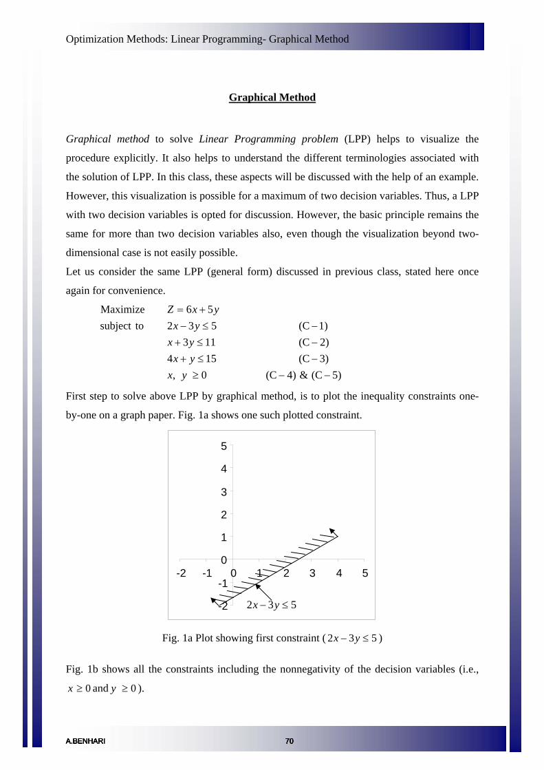
Optimization Methods: Linear Programming- Graphical Method
Graphical Method
Graphical method to solve Linear Programming problem (LPP) helps to visualize the
procedure explicitly. It also helps to understand the different terminologies associated with
the solution of LPP. In this class, these aspects will be discussed with the help of an example.
However, this visualization is possible for a maximum of two decision variables. Thus, a LPP
with two decision variables is opted for discussion. However, the basic principle remains the
same for more than two decision variables also, even though the visualization beyond two-
dimensional case is not easily possible.
Let us consider the same LPP (general form) discussed in previous class, stated here once
again for convenience.
5)(C&4)(C0,3)(C1542)(C1131)(C532tosubject
56Maximize
−−≥−≤+−≤+−≤−
+=
yxyxyx
yxyxZ
First step to solve above LPP by graphical method, is to plot the inequality constraints one-
by-one on a graph paper. Fig. 1a shows one such plotted constraint.
532 ≤− yx -2
-1
0
1
2
3
4
5
-2 -1 0 1 2 3 4 5
Fig. 1a Plot showing first constraint ( 532 ≤− yx )
Fig. 1b shows all the constraints including the nonnegativity of the decision variables (i.e.,
and ). 0≥x 0≥y
A.BENHARI 70A.BENHARI 70A.BENHARI 70A.BENHARI 70

Optimization Methods: Linear Programming- Graphical Method
113 ≤+ yx 154 ≤+ yx 0≥x 0≥y 532 ≤− yx
-2
-1
0
1
2
3
4
5
-2 -1 0 1 2 3 4 5
Fig. 1b Plot of all the constraints
Common region of all these constraints is known as feasible region (Fig. 1c). Feasible region
implies that each and every point in this region satisfies all the constraints involved in the
LPP.
-2
-1
0
1
2
3
4
5
-2 -1 0 1 2 3 4 5
Feasible region
Fig. 1c Feasible region
Once the feasible region is identified, objective function ( yxZ 56 += ) is to be plotted on it.
As the (optimum) value of Z is not known, objective function is plotted by considering any
constant, k (Fig. 1d). The straight line, kyx + =56 (constant), is known as Z line (Fig. 1d).
This line can be shifted in its perpendicular direction (as shown in the Fig. 1d) by changing
the value of k. Note that, position of Z line shown in Fig. 1d, showing the intercept, c, on the
A.BENHARI 71A.BENHARI 71A.BENHARI 71
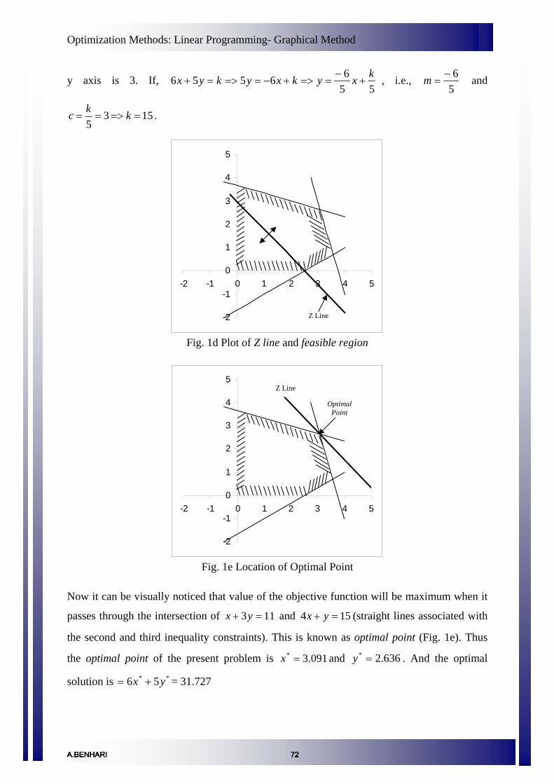
Optimization Methods: Linear Programming- Graphical Method
y axis is 3. If, 55
6556 xykxykyx +6 k−
==>+−==>=+ , i.e., 5
=m 6− and
1535
==>== kc k .
-2
3
4
5
-2 0 1 2 3 4 5-1
0
1
2
-1
Z Line
Fig. 1d Plot of Z line and feasible region
-2
-1
0
1
2
3
4
5
-2 -1 4 50 1 2 3
Optimal Point
Z Line
Fig. 1e Location of Optimal Point
Now it can be visually noticed that value of the objective function will be maximum when it
passes through the intersection of 113+ =yx 154 and + =yx
*x 636.2* =y** 56 yx +=
(straight lines associated with
the second and third inequality constraints). This is known as optimal point (Fig. 1e). Thus
the optimal point of the present problem is and . And the optimal
solution is = 31.727
091.3=
A.BENHARI 72A.BENHARI 72A.BENHARI 72
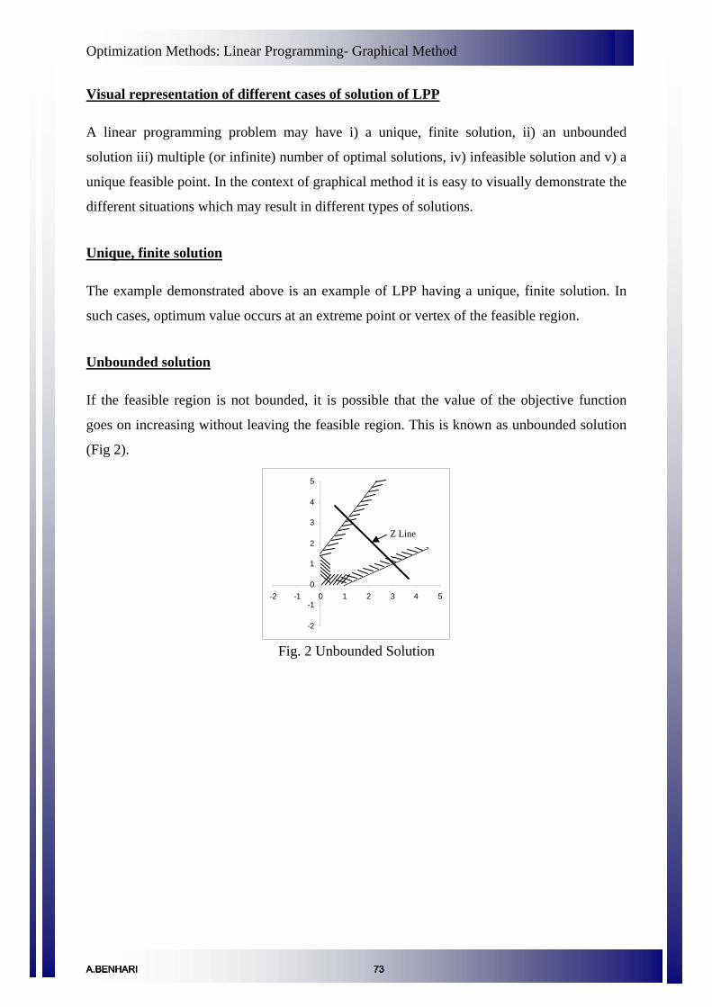
Optimization Methods: Linear Programming- Graphical Method
Visual representation of different cases of solution of LPP
A linear programming problem may have i) a unique, finite solution, ii) an unbounded
solution iii) multiple (or infinite) number of optimal solutions, iv) infeasible solution and v) a
unique feasible point. In the context of graphical method it is easy to visually demonstrate the
different situations which may result in different types of solutions.
Unique, finite solution
The example demonstrated above is an example of LPP having a unique, finite solution. In
such cases, optimum value occurs at an extreme point or vertex of the feasible region.
Unbounded solution
If the feasible region is not bounded, it is possible that the value of the objective function
goes on increasing without leaving the feasible region. This is known as unbounded solution
(Fig 2).
-2
-1
0
1
2
3
4
5
-2 -1 0 1 2 3 4 5
Z Line
Fig. 2 Unbounded Solution
A.BENHARI 73A.BENHARI 73A.BENHARI 73

Optimization Methods: Linear Programming- Graphical Method
Multiple (infinite) solutions
If the Z line is parallel to any side of the feasible region all the points lying on that side
constitute optimal solutions as shown in Fig 3.
-2
-1
0
1
2
3
4
5
-2 -1 0 1 2 3 4 5
Parallel
Z Line
Fig. 3 Multiple (infinite) Solution
Infeasible solution
Sometimes, the set of constraints does not form a feasible region at all due to inconsistency in
the constraints. In such situation the LPP is said to have infeasible solution. Fig 4 illustrates
such a situation.
-2
-1
0
1
2
3
4
5
-2 -1 0 1 2 3 4 5
Z Line
Fig. 4 Infeasible Solution
A.BENHARI 74A.BENHARI 74A.BENHARI 74

Optimization Methods: Linear Programming- Graphical Method
Unique feasible point
This situation arises when feasible region consist of a single point. This situation may occur
only when number of constraints is at least equal to the number of decision variables. An
example is shown in Fig 5. In this case, there is no need for optimization as there is only one
solution.
-2
-1
0
1
2
3
4
5
-2 -1 0 1 2 3 4 5
Unique feasible point
Fig. 5 Unique feasible point
A.BENHARI 75A.BENHARI 75A.BENHARI 75A.BENHARI 75

Optimization Methods: Linear Programming- Simplex Method-I
Simplex Method - I
Introduction
It is already stated in a previous lecture that the most popular method used for the solution of
Linear Programming Problems (LPP) is the simplex method. In this lecture, motivation for
simplex method will be discussed first. Simplex algorithm and construction of simplex
tableau will be discussed later with an example problem.
Motivation for Simplex method
Recall from the second class that the optimal solution of a LPP, if exists, lies at one of the
vertices of the feasible region. Thus one way to find the optimal solution is to find all the
basic feasible solutions of the canonical form and investigate them one-by-one to get at the
optimal. However, again recall the example at the end of the first class that, for 10 equations
with 15 variables there exists a huge number ( 1015c = 3003) of basic feasible solutions. In such
a case, inspection of all the solutions one-by-one is not practically feasible. However, this can
be overcome by simplex method. Conceptual principle of this method can be easily
understood for a three dimensional case (however, simplex method is applicable for any
higher dimensional case as well).
Imagine a feasible region (i.e., volume) bounded by several surfaces. Each vertex of this
volume, which is a basic feasible solution, is connected to three other adjacent vertices by a
straight line to each being the intersection of two surfaces. Being at any one vertex (one of
the basic feasible solutions), simplex algorithm helps to move to another adjacent vertex
which is closest to the optimal solution among all the adjacent vertices. Thus, it follows the
shortest route to reach the optimal solution from the starting point. It can be noted that the
shortest route consists of a sequence of basic feasible solutions which is generated by simplex
algorithm. The basic concept of simplex algorithm for a 3-D case is shown in Fig 1.
A.BENHARI 76A.BENHARI 76A.BENHARI 76A.BENHARI 76

Optimization Methods: Linear Programming- Simplex Method-I
Fig 1.
The general procedure of simplex method is as follows:
1. General form of given LPP is transformed to its canonical form (refer Lecture note 1).
2. A basic feasible solution of the LPP is found from the canonical form (there should
exist at least one).
3. This initial solution is moved to an adjacent basic feasible solution which is closest to
the optimal solution among all other adjacent basic feasible solutions.
4. The procedure is repeated until the optimum solution is achieved.
Step three involves simplex algorithm which is discussed in the next section.
Simplex algorithm
Simplex algorithm is discussed using an example of LPP. Let us consider the following
problem.
0,,
4225
024
622tosubject
24Maximize
321
321
321
321
321
≥
≤−−
≤+−
≤++
+−=
xxx
xxx
xxx
xxx
xxxZ
A.BENHARI 77A.BENHARI 77A.BENHARI 77

Optimization Methods: Linear Programming- Simplex Method-I
Simplex algorithm is used to obtain the solution of this problem. First let us transform the
LPP to its standard form as shown below.
0,,,,,
4225
024
622tosubject
24Maximize
654321
6321
5321
4321
321
≥
=+−−
=++−
=+++
+−=
xxxxxx
xxxx
xxxx
xxxx
xxxZ
It can be recalled that 4x , 5x and 6x are slack variables. Above set of equations, including the
objective function can be transformed to canonical form as follows:
4100225
001024
600122
000024
654321
654321
654321
654321
=+++−−
=++++−
=+++++
=++++−+−
xxxxxx
xxxxxx
xxxxxx
Zxxxxxx
The basic solution of above canonical form is 64 =x , 05 =x , 46 =x , 0321 === xxx and
0=Z . It can be noted that, 4x , 5x and 6x are known as basic variables and 321 and, xxx are
known as nonbasic variables of the canonical form shown above. Let us denote each equation
of above canonical form as:
( )( )( )( ) 4100225
001024
600122
000024
6543216
6543215
6543214
654321
=+++−−
=++++−
=+++++
=++++−+−
xxxxxxx
xxxxxxx
xxxxxxx
ZxxxxxxZ
For the ease of discussion, right hand side constants and the coefficients of the variables are
symbolized as follows:
( )( )( )( ) 65665654643632621616
55565554543532521515
45465454443432421414
565544332211
bxcxcxcxcxcxcxbxcxcxcxcxcxcxbxcxcxcxcxcxcxbZxcxcxcxcxcxcZ
=+++++=+++++=+++++=++++++
A.BENHARI 78A.BENHARI 78A.BENHARI 78

Optimization Methods: Linear Programming- Simplex Method-I
The left-most column is known as basis as this is consisting of basic variables. The
coefficients in the first row ( 61 cc Λ ) are known as cost coefficients. Other subscript notations
are self explanatory and used for the ease of discussion. For each coefficient, first subscript
indicates the subscript of the basic variable in that equation. Second subscript indicates the
subscript of variable with which the coefficient is associated. For example, 52c is the
coefficient of 2x in the equation having the basic variable 5x with nonzero coefficient (i.e.,
c55 is nonzero).
This completes first step of calculation. After completing each step (iteration) of calculation,
three points are to be examined:
1. Is there any possibility of further improvement?
2. Which nonbasic variable is to be entered into the basis?
3. Which basic variable is to be exited from the basis?
The procedure to check these points is discussed next.
1. Is there any possibility of further improvement?
If any of the cost coefficients is negative, further improvement is possible. In
other words, if all the cost coefficients are nonnegative, the basic feasible
solution obtained in that step is optimum.
2. Which nonbasic variable is to be entered?
Entering nonbasic variable is decided such that the unit change of this variable
should have maximum effect on the objective function. Thus the variable having
the coefficient which is minimum among all the cost coefficients is to be
entered, i.e., Sx is to be entered if cost coefficient Sc is minimum.
3. Which basic variable is to be exited?
After deciding the entering variable Sx , rx (from the set of basic variables) is
decided to be the exiting variable if rs
r
cb is minimum for all possible r, provided
rsc is positive.
A.BENHARI 79A.BENHARI 79A.BENHARI 79
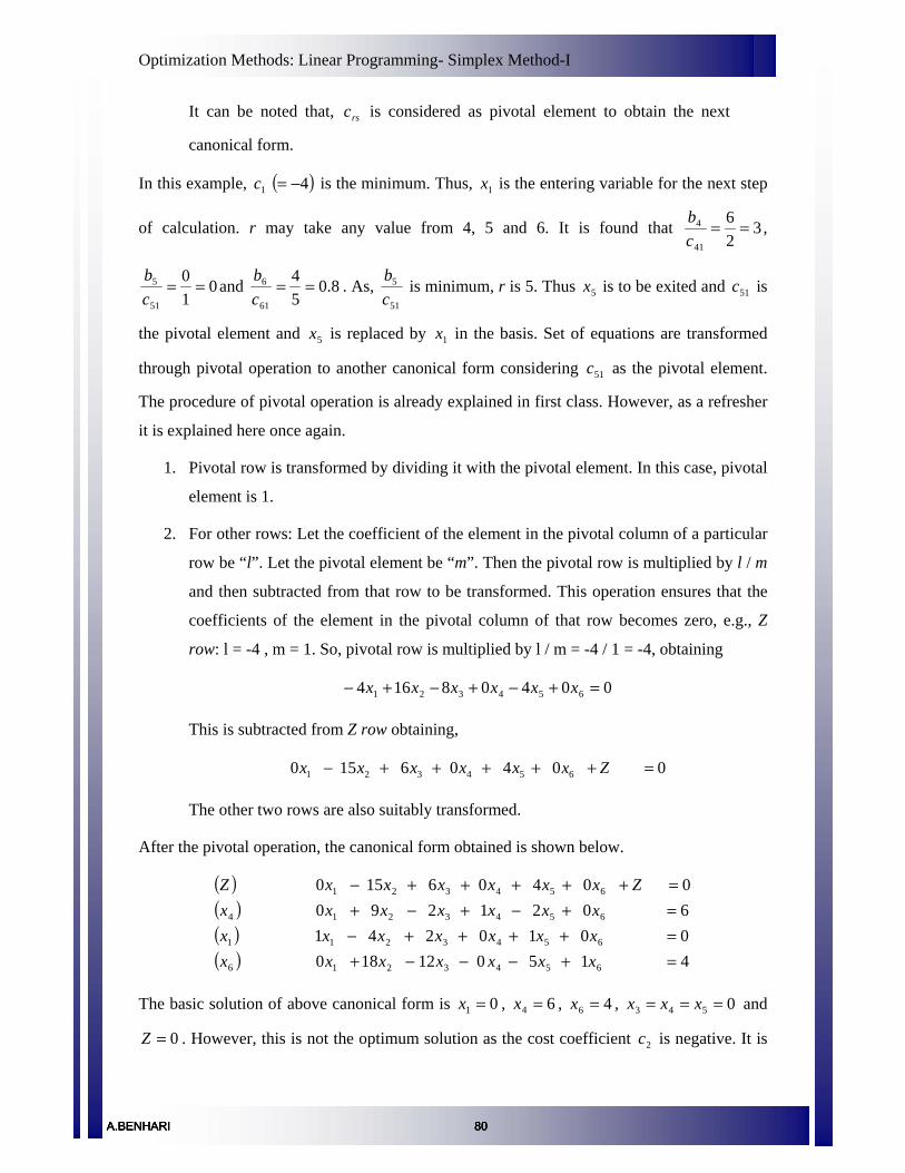
Optimization Methods: Linear Programming- Simplex Method-I
It can be noted that, rsc is considered as pivotal element to obtain the next
canonical form.
In this example, ( )41 −=c is the minimum. Thus, 1x is the entering variable for the next step
of calculation. r may take any value from 4, 5 and 6. It is found that 326
41
4 ==cb ,
010
51
5 ==cb
and 8.054
61
6 ==cb
. As, 51
5
cb
is minimum, r is 5. Thus 5x is to be exited and 51c is
the pivotal element and 5x is replaced by 1x in the basis. Set of equations are transformed
through pivotal operation to another canonical form considering 51c as the pivotal element.
The procedure of pivotal operation is already explained in first class. However, as a refresher
it is explained here once again.
1. Pivotal row is transformed by dividing it with the pivotal element. In this case, pivotal
element is 1.
2. For other rows: Let the coefficient of the element in the pivotal column of a particular
row be “l”. Let the pivotal element be “m”. Then the pivotal row is multiplied by l / m
and then subtracted from that row to be transformed. This operation ensures that the
coefficients of the element in the pivotal column of that row becomes zero, e.g., Z
row: l = -4 , m = 1. So, pivotal row is multiplied by l / m = -4 / 1 = -4, obtaining
00408164 654321 =+−+−+− xxxxxx
This is subtracted from Z row obtaining,
00406150 654321 =+++++− Zxxxxxx
The other two rows are also suitably transformed.
After the pivotal operation, the canonical form obtained is shown below.
( )( )( )( ) 415012180
0010241602129000406150
6543216
6543211
6543214
654321
=+−−−+=++++−=+−+−+=+++++−
xxxxxxxxxxxxxxxxxxxxx
ZxxxxxxZ
The basic solution of above canonical form is 01 =x , 64 =x , 46 =x , 0543 === xxx and
0=Z . However, this is not the optimum solution as the cost coefficient 2c is negative. It is
A.BENHARI 80A.BENHARI 80A.BENHARI 80
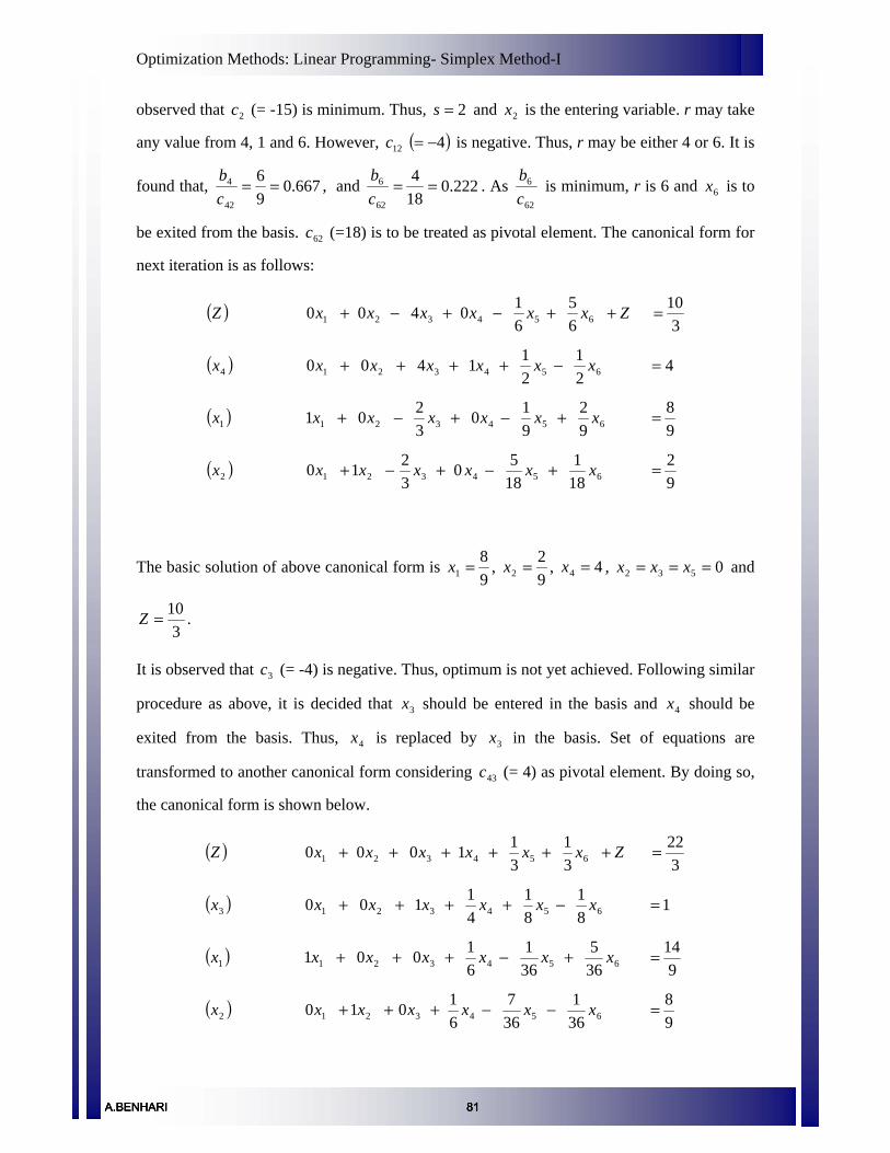
Optimization Methods: Linear Programming- Simplex Method-I
observed that 2c (= -15) is minimum. Thus, 2=s and 2x is the entering variable. r may take
any value from 4, 1 and 6. However, ( )412 −=c is negative. Thus, r may be either 4 or 6. It is
found that, 667.096
42
4 ==cb , and 222.0
184
62
6 ==cb
. As 62
6
cb
is minimum, r is 6 and 6x is to
be exited from the basis. 62c (=18) is to be treated as pivotal element. The canonical form for
next iteration is as follows:
( )
( )
( )
( )92
181
1850
3210
98
92
910
3201
421
211400
310
65
610400
6543212
6543211
6543214
654321
=+−+−+
=+−+−+
=−++++
=++−+−+
xxxxxxx
xxxxxxx
xxxxxxx
ZxxxxxxZ
The basic solution of above canonical form is 98
1 =x , 92
2 =x , 44 =x , 0532 === xxx and
310=Z .
It is observed that 3c (= -4) is negative. Thus, optimum is not yet achieved. Following similar
procedure as above, it is decided that 3x should be entered in the basis and 4x should be
exited from the basis. Thus, 4x is replaced by 3x in the basis. Set of equations are
transformed to another canonical form considering 43c (= 4) as pivotal element. By doing so,
the canonical form is shown below.
( )
( )
( )
( )98
361
367
61010
914
365
361
61001
181
81
41100
322
31
311000
6543212
6543211
6543213
654321
=−−+++
=+−+++
=−++++
=++++++
xxxxxxx
xxxxxxx
xxxxxxx
ZxxxxxxZ
A.BENHARI 81A.BENHARI 81A.BENHARI 81

Optimization Methods: Linear Programming- Simplex Method-I
The basic solution of above canonical form is 9
141 =x ,
98
2 =x , 13 =x , 0654 === xxx and
322=Z .
It is observed that all the cost coefficients are positive. Thus, optimum is achieved. Hence,
the optimum solution is
333.7322 ==Z
556.19
141 ==x
889.098
2 ==x
13 =x
The calculation shown above can be presented in a tabular form, which is known as Simplex
Tableau. Construction of Simplex Tableau will be discussed next.
Construction of Simplex Tableau
Same LPP is considered for the construction of simplex tableau. This helps to compare the
calculation shown above and the construction of simplex tableau for it.
After preparing the canonical form of the given LPP, simplex tableau is constructed as
follows.
A.BENHARI 82A.BENHARI 82A.BENHARI 82

Optimization Methods: Linear Programming- Simplex Method-I
Variables Iteration Basis Z
1x 2x 3x 4x 5x 6x rb
rs
r
cb
Z 1 -4 1 -2 0 0 0 0 --
4x 0 2 1 2 1 0 0 6 3
5x 0 1 -4 2 0 1 0 0 0 1
6x 0 5 -2 -2 0 0 1 4 54
After completing each iteration, the steps given below are to be followed.
Logically, these steps are exactly similar to the procedure described earlier. However, steps
described here are somewhat mechanical and easy to remember!
Check for optimum solution:
1. Investigate whether all the elements in the first row (i.e., Z row) are nonnegative or
not. Basically these elements are the coefficients of the variables headed by that
column. If all such coefficients are nonnegative, optimum solution is obtained and no
need of further iterations. If any element in this row is negative, the operation to
obtain simplex tableau for the next iteration is as follows:
Operations to obtain next simplex tableau:
2. The entering variable is identified (described earlier). The corresponding column is
marked as Pivotal Column as shown above.
3. The exiting variable from the basis is identified (described earlier). The corresponding
row is marked as Pivotal Row as shown above.
4. Coefficient at the intersection of Pivotal Row and Pivotal Column is marked as
Pivotal Element as shown above.
5. In the basis, the exiting variable is replaced by entering variable.
Pivotal Column
Pivotal Element
Pivotal Row
A.BENHARI 83A.BENHARI 83A.BENHARI 83

Optimization Methods: Linear Programming- Simplex Method-I
6. All the elements in the pivotal row are divided by pivotal element.
7. For any other row, an elementary operation is identified such that the coefficient in
the pivotal column in that row becomes zero. The same operation is applied for all
other elements in that row and the coefficients are changed accordingly. A similar
procedure is followed for all other rows.
For example, say, (2 x pivotal element + pivotal coefficient in first row) produce zero
in the pivotal column in first row. The same operation is applied for all other elements
in the first row and the coefficients are changed accordingly.
Simplex tableaus for successive iterations are shown below. Pivotal Row, Pivotal Column
and Pivotal Element for each tableau are marked as earlier for the ease of understanding.
Variables Iteration Basis Z
1x 2x 3x 4x 5x 6x rb
rs
r
cb
Z 1 0 -15 6 0 4 0 0 --
4x 0 0 9 -2 1 -2 0 6 31
1x 0 1 -4 2 0 1 0 0 -- 2
6x 0 0 18 -12 0 -5 1 4 92
……continued to next page
A.BENHARI 84A.BENHARI 84A.BENHARI 84

Optimization Methods: Linear Programming- Simplex Method-I
……continued from previous page
Variables Iteration Basis Z
1x 2x 3x 4x 5x 6x rb
rs
r
cb
Z 1 0 0 -4 0 61−
65
310 --
4x 0 0 0 4 1 21
21− 4 1
1x 0 1 0 32− 0
91−
92
98 --
3
2x 0 0 1 32− 0
185−
181
92 --
Z 1 0 0 0 1 31
31
322
3x 0 0 0 1 41
81
81− 1
1x 0 1 0 0 61
361−
92
914
4
2x 0 0 1 0 61
367−
361−
98
Optimum value of Z
Value of 3x Value of 1x Value of 2x
All the coefficients are nonnegative. Thus optimum solution is achieved.
A.BENHARI 85A.BENHARI 85A.BENHARI 85

Optimization Methods: Linear Programming- Simplex Method-I
As all the elements in the first row (i.e., Z row), at iteration 4, are nonnegative, optimum
solution is achieved. Optimum value of Z is 333.7322 = as shown above. Corresponding
values of basic variables are 556.19
141 ==x , 889.0
98
2 ==x , 13 =x and those of nonbasic
variables are all zero (i.e., 0654 === xxx ).
It can be noted that at any iteration the following two points must be satisfied:
1. All the basic variables (other than Z) have a coefficient of zero in the Z row.
2. Coefficients of basic variables in other rows constitute a unit matrix.
If any of these points are violated at any iteration, it indicates a wrong calculation. However,
reverse is not true.
A.BENHARI 86A.BENHARI 86A.BENHARI 86A.BENHARI 86

Optimization Methods: Linear Programming- Simplex Method - II
Simplex Method – II
Introduction
In the previous lecture the simplex method was discussed with required transformation of
objective function and constraints. However, all the constraints were of inequality type with
‘less-than-equal-to’ ( ≤ ) sign. However, ‘greater-than-equal-to’ ( ≥ ) and ‘equality’ ( = )
constraints are also possible. In such cases, a modified approach is followed, which will be
discussed in this lecture. Different types of LPP solutions in the context of Simplex method
will also be discussed. Finally, a discussion on minimization vs maximization will be
presented.
Simplex Method with ‘greater-than-equal-to’ ( ≥ ) and equality ( = ) constraints
The LP problem, with ‘greater-than-equal-to’ ( ≥ ) and equality ( = ) constraints, is transformed
to its standard form in the following way.
1. One ‘artificial variable’ is added to each of the ‘greater-than-equal-to’ ( ≥ ) and equality
( = ) constraints to ensure an initial basic feasible solution.
2. Artificial variables are ‘penalized’ in the objective function by introducing a large
negative (positive) coefficient M for maximization (minimization) problem.
3. Cost coefficients, which are supposed to be placed in the Z-row in the initial simplex
tableau, are transformed by ‘pivotal operation’ considering the column of artificial
variable as ‘pivotal column’ and the row of the artificial variable as ‘pivotal row’.
4. If there are more than one artificial variable, step 3 is repeated for all the artificial
variables one by one.
Let us consider the following LP problem
1 2
1 2
2
1 2
1 2
Maximize 3 5subject to 2
63 2 18
, 0
Z x xx xxx x
x x
= ++ ≥≤+ =
≥
After incorporating the artificial variables, the above LP problem becomes as follows:
A.BENHARI 87A.BENHARI 87A.BENHARI 87A.BENHARI 87

Optimization Methods: Linear Programming- Simplex Method - II
1 2 1 2
1 2 3 1
2 4
1 2 2
1 2
Maximize 3 5subject to 2
63 2 18
, 0
Z x x Ma Max x x ax xx x a
x x
= + − −+ − + =+ =+ + =
≥
where 3x is surplus variable, 4x is slack variable and 1a and 2a are the artificial variables.
Cost coefficients in the objective function are modified considering the first constraint as
follows:
( )( )
1 2 1 2 1
1 2 3 1 2
3 5 0
2
Z x x Ma Ma E
x x x a E
− − + + =
+ − + =
Thus, pivotal operation is 21 EME ×− , which modifies the cost coefficients as follows:
( ) ( ) MMaaMxxMxMZ 2053 21321 −=++++−+−
Next, the revised objective function is considered with third constraint as follows:
( ) ( ) ( )( )4221
321321
1823
2053
Eaxx
EMMaaMxxMxMZ
=++
−=++++−+−
Obviously pivotal operation is 43 EME ×− , which further modifies the cost coefficients as
follows:
( ) ( ) MaaMxxMxMZ 20003543 21321 −=++++−+−
The modified cost coefficients are to be used in the Z-row of the first simplex tableau.
Next, let us move to the construction of simplex tableau. Pivotal column, pivotal row and
pivotal element are marked (same as used in the last class) for the ease of understanding.
Pivotal Column
Pivotal Row
Pivotal Column
Pivotal Row
A.BENHARI 88A.BENHARI 88A.BENHARI 88
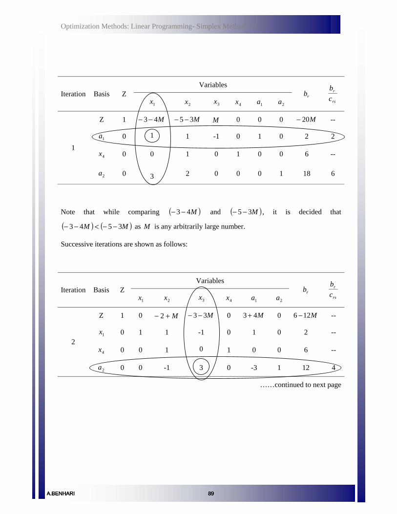
Optimization Methods: Linear Programming- Simplex Method - II
Variables Iteration Basis Z
1x 2x 3x 4x 1a 2a rb
rs
r
cb
Z 1 M43 −− M35 −− M 0 0 0 M20− --
1a 0 1 1 -1 0 1 0 2 2
4x 0 0 1 0 1 0 0 6 -- 1
2a 0 3 2 0 0 0 1 18 6
Note that while comparing ( )M43 −− and ( )M35 −− , it is decided that
( ) ( )MM 3543 −−<−− as M is any arbitrarily large number.
Successive iterations are shown as follows:
Variables Iteration Basis Z
1x 2x 3x 4x 1a 2a rb
rs
r
cb
Z 1 0 M+− 2 M33 −− 0 M43 + 0 M126 − --
1x 0 1 1 -1 0 1 0 2 --
4x 0 0 1 0 1 0 0 6 -- 2
2a 0 0 -1 3 0 -3 1 12 4
……continued to next page
A.BENHARI 89A.BENHARI 89A.BENHARI 89

Optimization Methods: Linear Programming- Simplex Method - II
……continuing from previous page
Variables Iteration Basis Z
1x 2x 3x 4x 1a 2a rb
rs
r
cb
Z 1 0 -3 0 0 M M+1 18 --
1x 0 1 32 0 0 0
13
6 9
4x 0 0 1 0 1 0 0 6 6 3
3x 0 0 31− 1 0 -1
31 4 --
Z 1 0 0 0 3 M M+1 36 --
1x 0 1 0 0 23
− 0 13
2 --
2x 0 0 1 0 1 0 0 6 -- 4
3x 0 0 0 1 31 -1
31 6 --
It is found that, at iteration 4, optimality has reached. Optimal solution is 36Z = with 1 2x =
and 2 6x = . The methodology explained above is known as Big-M method. Hope, reader has
already understood the meaning of the terminology!
‘Unbounded’, ‘Multiple’ and ‘Infeasible’ solutions in the context of Simplex Method
As already discussed in lecture notes 2, a linear programming problem may have different type
of solutions corresponding to different situations. Visual demonstration of these different types
of situations was also discussed in the context of graphical method. Here, the same will be
discussed in the context of Simplex method.
A.BENHARI 90A.BENHARI 90A.BENHARI 90

Optimization Methods: Linear Programming- Simplex Method - II
Unbounded solution
If at any iteration no departing variable can be found corresponding to entering variable, the
value of the objective function can be increased indefinitely, i.e., the solution is unbounded.
Multiple (infinite) solutions
If in the final tableau, one of the non-basic variables has a coefficient 0 in the Z-row, it
indicates that an alternative solution exists. This non-basic variable can be incorporated in the
basis to obtain another optimal solution. Once two such optimal solutions are obtained, infinite
number of optimal solutions can be obtained by taking a weighted sum of the two optimal
solutions.
Consider the slightly revised above problem,
1 2
1 2
2
1 2
1 2
Maximize 3 2subject to 2
63 2 18
, 0
Z x xx xxx x
x x
= ++ ≥≤+ =
≥
Curious readers may find that the only modification is that the coefficient of 2x is changed
from 5 to 2 in the objective function. Thus the slope of the objective function and that of third
constraint are now same. It may be recalled from lecture notes 2, that if the Z line is parallel to
any side of the feasible region (i.e., one of the constraints) all the points lying on that side
constitute optimal solutions (refer fig 3 in lecture notes 2). So, reader should be able to imagine
graphically that the LPP is having infinite solutions. However, for this particular set of
constraints, if the objective function is made parallel (with equal slope) to either the first
constraint or the second constraint, it will not lead to multiple solutions. The reason is very
simple and left for the reader to find out. As a hint, plot all the constraints and the objective
function on an arithmetic paper.
Now, let us see how it can be found in the simplex tableau. Coming back to our problem, final
tableau is shown as follows. Full problem is left to the reader as practice.
A.BENHARI 91A.BENHARI 91A.BENHARI 91

Optimization Methods: Linear Programming- Simplex Method - II
Final tableau:
Variables Iteration Basis Z
1x 2x 3x 4x 1a 2a rb
rs
r
cb
Z 1 0 0 0 0 M M+1 18 --
1x 0 1 32 0 0 0
13
6 9
4x 0 0 1 0 1 0 0 6 6 3
3x 0 0 31− 1 0 -1
31 4 --
As there is no negative coefficient in the Z-row the optimal is reached. The solution is 18Z =
with 1 6x = and 2 0x = . However, the coefficient of non-basic variable 2x is zero as shown in
the final simplex tableau. So, another solution is possible by incorporating 2x in the basis.
Based on the rs
r
cb , 4x will be the exiting variable. The next tableau will be as follows:
Variables Iteration Basis Z
1x 2x 3x 4x 1a 2a rb
rs
r
cb
Z 1 0 0 0 0 M M+1 18 --
1x 0 1 0 0 23
− 0 13
2 --
2x 0 0 1 0 1 0 0 6 6 4
3x 0 0 0 1 31 -1
31 6 18
Thus, another solution is obtained, which is 18Z = with 1 2x = and 2 6x = . Again, it may be
noted that, the coefficient of non-basic variable 4x is zero as shown in the tableau. If one more
similar step is performed, same simplex tableau at iteration 3 will be obtained.
Coefficient of non-basic variable 2x is zero
Coefficient of non-basic variable 4x is zero
A.BENHARI 92A.BENHARI 92A.BENHARI 92
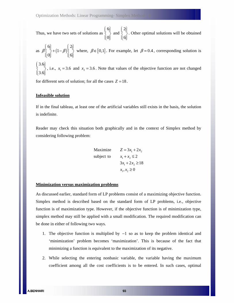
Optimization Methods: Linear Programming- Simplex Method - II
Thus, we have two sets of solutions as 6
0
⎧ ⎫⎪ ⎪⎨ ⎬⎪ ⎪⎩ ⎭
and 2
6
⎧ ⎫⎪ ⎪⎨ ⎬⎪ ⎪⎩ ⎭
. Other optimal solutions will be obtained
as ( )6 2
10 6
β β⎧ ⎫ ⎧ ⎫⎪ ⎪ ⎪ ⎪+ −⎨ ⎬ ⎨ ⎬⎪ ⎪ ⎪ ⎪⎩ ⎭ ⎩ ⎭
where, [ ]0,1β ∈ . For example, let 0.4β = , corresponding solution is
3.6
3.6
⎧ ⎫⎪ ⎪⎨ ⎬⎪ ⎪⎩ ⎭
, i.e., 1 3.6x = and 2 3.6x = . Note that values of the objective function are not changed
for different sets of solution; for all the cases 18Z = .
Infeasible solution
If in the final tableau, at least one of the artificial variables still exists in the basis, the solution
is indefinite.
Reader may check this situation both graphically and in the context of Simplex method by
considering following problem:
1 2
1 2
1 2
1 2
Maximize 3 2subject to 2
3 2 18, 0
Z x xx xx x
x x
= ++ ≤+ ≥
≥
Minimization versus maximization problems
As discussed earlier, standard form of LP problems consist of a maximizing objective function.
Simplex method is described based on the standard form of LP problems, i.e., objective
function is of maximization type. However, if the objective function is of minimization type,
simplex method may still be applied with a small modification. The required modification can
be done in either of following two ways.
1. The objective function is multiplied by 1− so as to keep the problem identical and
‘minimization’ problem becomes ‘maximization’. This is because of the fact that
minimizing a function is equivalent to the maximization of its negative.
2. While selecting the entering nonbasic variable, the variable having the maximum
coefficient among all the cost coefficients is to be entered. In such cases, optimal
A.BENHARI 93A.BENHARI 93A.BENHARI 93

Optimization Methods: Linear Programming- Simplex Method - II
solution would be determined from the tableau having all the cost coefficients as non-
positive ( 0≤ )
Still one difficulty remains in the minimization problem. Generally the minimization problems
consist of constraints with ‘greater-than-equal-to’ ( ≥ ) sign. For example, minimize the price
(to compete in the market); however, the profit should cross a minimum threshold. Whenever
the goal is to minimize some objective, lower bounded requirements play the leading role.
Constraints with ‘greater-than-equal-to’ ( ≥ ) sign are obvious in practical situations.
To deal with the constraints with ‘greater-than-equal-to’ ( ≥ ) and = sign, Big-M method is to
be followed as explained earlier.
A.BENHARI 94A.BENHARI 94A.BENHARI 94

Optimization Methods: Linear Programming- Revised Simplex Method
Revised Simplex Method, Duality and Sensitivity analysis
Introduction
In the previous class, the simplex method was discussed where the simplex tableau at each
iteration needs to be computed entirely. However, revised simplex method is an improvement
over simplex method. Revised simplex method is computationally more efficient and accurate.
Duality of LP problem is a useful property that makes the problem easier in some cases and
leads to dual simplex method. This is also helpful in sensitivity or post optimality analysis of
decision variables.
In this lecture, revised simplex method, duality of LP, dual simplex method and sensitivity or
post optimality analysis will be discussed.
Revised Simplex method
Benefit of revised simplex method is clearly comprehended in case of large LP problems. In
simplex method the entire simplex tableau is updated while a small part of it is used. The
revised simplex method uses exactly the same steps as those in simplex method. The only
difference occurs in the details of computing the entering variables and departing variable as
explained below.
Let us consider the following LP problem, with general notations, after transforming it to its
standard form and incorporating all required slack, surplus and artificial variables.
( )( )( )
( )
1 1 2 2 3 3
11 1 12 2 13 3 1 1
21 1 22 2 23 3 2 2
1 1 2 2 3 3
0n n
i n n
j n n
l m m m mn n m
Z c x c x c x c x Z
x c x c x c x c x b
x c x c x c x c x b
x c x c x c x c x b
+ + + + + =
+ + + + =
+ + + + =
+ + + + =
L L L
L L L
L L L
M M MM M M
L L L
As the revised simplex method is mostly beneficial for large LP problems, it will be
discussed in the context of matrix notation. Matrix notation of above LP problem can be
expressed as follows:
A.BENHARI 95A.BENHARI 95A.BENHARI 95A.BENHARI 95
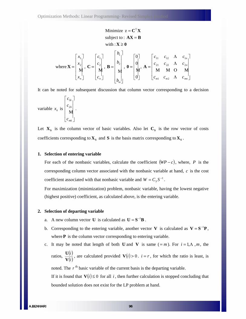
Optimization Methods: Linear Programming- Revised Simplex Method
:with :subject toz Minimize T
0XBAXXC
≥=
=
where
⎥⎥⎥⎥
⎦
⎤
⎢⎢⎢⎢
⎣
⎡
=
nx
xx
Μ2
1
X ,
⎥⎥⎥⎥
⎦
⎤
⎢⎢⎢⎢
⎣
⎡
=
nc
cc
Μ2
1
C ,
1
2
m
b
b
b
⎡ ⎤⎢ ⎥⎢ ⎥⎢ ⎥=⎢ ⎥⎢ ⎥⎢ ⎥⎣ ⎦
BM
,
⎥⎥⎥⎥
⎦
⎤
⎢⎢⎢⎢
⎣
⎡
=
0
00
Μ0 ,
⎥⎥⎥⎥
⎦
⎤
⎢⎢⎢⎢
⎣
⎡
=
mnmm
n
n
ccc
cccccc
ΛΜΟΜΜ
ΛΛ
21
22221
11211
A
It can be noted for subsequent discussion that column vector corresponding to a decision
variable kx is
⎥⎥⎥⎥
⎦
⎤
⎢⎢⎢⎢
⎣
⎡
mk
k
k
c
cc
Μ2
1
.
Let SX is the column vector of basic variables. Also let SC is the row vector of costs
coefficients corresponding to SX and S is the basis matrix corresponding to SX .
1. Selection of entering variable
For each of the nonbasic variables, calculate the coefficient ( )cWP − , where, P is the
corresponding column vector associated with the nonbasic variable at hand, c is the cost
coefficient associated with that nonbasic variable and 1−= SCW S .
For maximization (minimization) problem, nonbasic variable, having the lowest negative
(highest positive) coefficient, as calculated above, is the entering variable.
2. Selection of departing variable
a. A new column vector U is calculated as BSU 1−= .
b. Corresponding to the entering variable, another vector V is calculated as PSV 1−= ,
where P is the column vector corresponding to entering variable.
c. It may be noted that length of both U and V is same ( m= ). For mi ,,1 Λ= , the
ratios, ( )( )ii
VU , are calculated provided ( ) 0>iV . ri = , for which the ratio is least, is
noted. The r th basic variable of the current basis is the departing variable.
If it is found that ( ) 0≤iV for all i , then further calculation is stopped concluding that
bounded solution does not exist for the LP problem at hand.
A.BENHARI 96A.BENHARI 96A.BENHARI 96

Optimization Methods: Linear Programming- Revised Simplex Method
3. Update to new basis
Old basis S , is updated to new basis newS , as [ ] 11 −−= ESS new
where
1
2
1
1 0 0 0
0 1 0 0
0 0 1 0
0 0 0 1
r
m
m
η
η
η
η
η
−
⎡ ⎤⎢ ⎥⎢ ⎥⎢ ⎥⎢ ⎥⎢ ⎥⎢ ⎥=⎢ ⎥⎢ ⎥⎢ ⎥⎢ ⎥⎢ ⎥⎢ ⎥⎣ ⎦
E
L L
L L
M M O M L M M
M M L L M M
M M L M O M M
L L
L L
and
( )( )
( )⎪⎪⎩
⎪⎪⎨
⎧
=
≠=
rirV
rirViV
i
for1
forη
S is replaced by newS and steps 1 through 3 are repeated. If all the coefficients calculated in
step 1, i.e., ( )cWP − is positive (negative) in case of maximization (minimization) problem,
then optimum solution is reached and the optimal solution is,
BSXS1−= and SCX=z
Duality of LP problems
Each LP problem (called as Primal in this context) is associated with its counterpart known
as Dual LP problem. Instead of primal, solving the dual LP problem is sometimes easier
when a) the dual has fewer constraints than primal (time required for solving LP problems is
directly affected by the number of constraints, i.e., number of iterations necessary to
converge to an optimum solution which in Simplex method usually ranges from 1.5 to 3
times the number of structural constraints in the problem) and b) the dual involves
maximization of an objective function (it may be possible to avoid artificial variables that
otherwise would be used in a primal minimization problem).
The dual LP problem can be constructed by defining a new decision variable for each
constraint in the primal problem and a new constraint for each variable in the primal. The
coefficients of the j th variable in the dual’s objective function is the i th component of the
primal’s requirements vector (right hand side values of the constraints in the Primal). The
dual’s requirements vector consists of coefficients of decision variables in the primal
objective function. Coefficients of each constraint in the dual (i.e., row vectors) are the
r th column
A.BENHARI 97A.BENHARI 97A.BENHARI 97
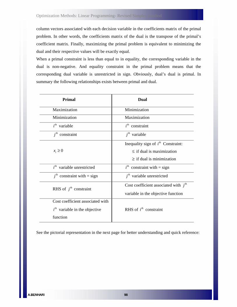
Optimization Methods: Linear Programming- Revised Simplex Method
column vectors associated with each decision variable in the coefficients matrix of the primal
problem. In other words, the coefficients matrix of the dual is the transpose of the primal’s
coefficient matrix. Finally, maximizing the primal problem is equivalent to minimizing the
dual and their respective values will be exactly equal.
When a primal constraint is less than equal to in equality, the corresponding variable in the
dual is non-negative. And equality constraint in the primal problem means that the
corresponding dual variable is unrestricted in sign. Obviously, dual’s dual is primal. In
summary the following relationships exists between primal and dual.
Primal Dual
Maximization Minimization
Minimization Maximization thi variable thi constraint thj constraint thj variable
0ix ≥ Inequality sign of thi Constraint:
≤ if dual is maximization
≥ if dual is minimization thi variable unrestricted thi constraint with = sign thj constraint with = sign thj variable unrestricted
RHS of thj constraint Cost coefficient associated with thj
variable in the objective function
Cost coefficient associated with thi variable in the objective
function
RHS of thi constraint
See the pictorial representation in the next page for better understanding and quick reference:
A.BENHARI 98A.BENHARI 98A.BENHARI 98

Optimization Methods: Linear Programming- Revised Simplex Method
Coefficients of the 2nd constraint
Determine the sign of 1y
Determine the sign of 2y
1 1 2 2
11 1 12 2 1 1 1
21 1 22 2 2 2 2
1 1 2 2
1 2
Maximize
Subject to
0, unrestricted, , 0
n n
n n
n n
m m mn n m m
n
Z c x c x c x
c x c x c x b y
c x c x c x b y
c x c x c x b yx x x
= + + +
+ + + = ⎯⎯→
+ + + ≤ ⎯⎯→
+ + + ≤ ⎯⎯→≥ ≥
L L L
L L L
L L LM M
L L LL
M M M M
L L
1 1 2 2
11 1 21 2 1 1
12 1 22 2 2 2
1 1 2 2
1 2
MinimizeSubject to
unrestricted, 0, , 0
m m
m m
m m
n n mn m n
m
Z b y b y b yc y c y c y cc y c y c y c
c y c y c y cy y y
= + + ++ + + ≤+ + + =
+ + + ≤≥ ≥
L L LL L LL L L
M ML L L
L
Opposite for the Dual, i.e., Minimize
Cost coefficients for the Objective Function
Mark the corresponding decision variables in the dual
Coefficients of the 1st
constraint
Corresponding sign of the 1st
constraint is ≤
Right hand side of the 1st
constraint
Thus the Objective Function, 1 1 2 2Minimize m mb y b y b y+ + +L
Thus, the 1st constraint, 11 1 21 2 1 1m mc y c y c y c+ + + ≤L
Corresponding sign of the 2nd constraint is =
Right hand side of the 2nd
constraint
Thus, the 2nd constraint, 12 1 22 2 2 2m mc y c y c y c+ + + =L
Dual Problem
Determine the sign of my
A.BENHARI 99A.BENHARI 99A.BENHARI 99

Optimization Methods: Linear Programming- Revised Simplex Method
It may be noted that, before finding its dual, all the constraints should be transformed to ‘less-
than-equal-to’ or ‘equal-to’ type for maximization problem and to ‘greater-than-equal-to’ or
‘equal-to’ type for minimization problem. It can be done by multiplying with 1− both sides
of the constraints, so that inequality sign gets reversed.
An example of finding dual problem is illustrated with the following example.
Primal Dual
Maximize 21 34 xxZ += Minimize 321 400020006000 yyyZ +−=′
Subject to
600032
21 ≤+ xx
200021 ≥− xx
40001 ≤x
1x unrestricted
02 ≥x
Subject to
4321 =+− yyy
332
21 ≤+ yy
01 ≥y
02 ≥y
03 ≥y
It may be noted that second constraint in the primal is transformed to 1 2 2000x x− + ≤ −
before constructing the dual.
Primal-Dual relationships
Following points are important to be noted regarding primal-dual relationship:
1. If one problem (either primal or dual) has an optimal feasible solution, other problem
also has an optimal feasible solution. The optimal objective function value is same for
both primal and dual.
2. If one problem has no solution (infeasible), the other problem is either infeasible or
unbounded.
3. If one problem is unbounded the other problem is infeasible.
A.BENHARI 100A.BENHARI 100A.BENHARI 100

Optimization Methods: Linear Programming- Revised Simplex Method
Dual Simplex Method
Computationally, dual simplex method is same as simplex method. However, their
approaches are different from each other. Simplex method starts with a nonoptimal but
feasible solution where as dual simplex method starts with an optimal but infeasible solution.
Simplex method maintains the feasibility during successive iterations where as dual simplex
method maintains the optimality. Steps involved in the dual simplex method are:
1. All the constraints (except those with equality (=) sign) are modified to ‘less-than-
equal-to’ ( ≤ ) sign. Constraints with greater-than-equal-to’ ( ≥ ) sign are multiplied by
1− through out so that inequality sign gets reversed. Finally, all these constraints are
transformed to equality (=) sign by introducing required slack variables.
2. Modified problem, as in step one, is expressed in the form of a simplex tableau. If all
the cost coefficients are positive (i.e., optimality condition is satisfied) and one or
more basic variables have negative values (i.e., non-feasible solution), then dual
simplex method is applicable.
3. Selection of exiting variable: The basic variable with the highest negative value is
the exiting variable. If there are two candidates for exiting variable, any one is
selected. The row of the selected exiting variable is marked as pivotal row.
4. Selection of entering variable: Cost coefficients, corresponding to all the negative
elements of the pivotal row, are identified. Their ratios are calculated after changing
the sign of the elements of pivotal row, i.e., ⎟⎟⎠
⎞⎜⎜⎝
⎛×−
=rowpivotalofElements
tsCoefficienCostratio1
.
The column corresponding to minimum ratio is identified as the pivotal column and
associated decision variable is the entering variable.
5. Pivotal operation: Pivotal operation is exactly same as in the case of simplex
method, considering the pivotal element as the element at the intersection of pivotal
row and pivotal column.
6. Check for optimality: If all the basic variables have nonnegative values then the
optimum solution is reached. Otherwise, Steps 3 to 5 are repeated until the optimum is
reached.
A.BENHARI 101A.BENHARI 101A.BENHARI 101

Optimization Methods: Linear Programming- Revised Simplex Method
Consider the following problem:
1212342443
2tosubject2Minimize
21
21
21
1
21
≥+−≥+≤+
≥+=
xxxxxx
xxxZ
By introducing the surplus variables, the problem is reformulated with equality constraints as
follows:
121234
24432tosubject
2Minimize
621
521
421
31
21
−=+−−=+−−
=++−=+−
+=
xxxxxxxxxxx
xxZ
Expressing the problem in the tableau form:
Variables Iteration Basis Z
1x 2x 3x 4x 5x 6x rb
Z 1 -2 -1 0 0 0 0 0
3x 0 -1 0 1 0 0 0 -2
4x 0 3 4 0 1 0 0 24
5x 0 -4 -3 0 0 1 0 -12
1
6x 0 1 -2 0 0 0 1 -1
Ratios 0.5 1/3 -- -- 0 --
Pivotal Column
Pivotal ElementPivotal Row
A.BENHARI 102A.BENHARI 102A.BENHARI 102

Optimization Methods: Linear Programming- Revised Simplex Method
Tableaus for successive iterations are shown below. Pivotal Row, Pivotal Column and Pivotal
Element for each tableau are marked as usual.
Variables Iteration Basis
Z 1x 2x 3x 4x 5x 6x rb
Z 1 -2/3 0 0 0 -1/3 0 4
3x 0 -1 0 1 0 0 0 -2
4x 0 -7/3 0 0 1 4/3 0 8
2x 0 4/3 1 0 0 -1/3 0 4
2
6x 0 11/3 0 0 0 -2/3 1 7
Ratios 2/3 -- -- -- -- --
Variables
Iteration Basis Z 1x 2x 3x 4x 5x 6x rb
Z 1 0 0 -2/3 0 -1/3 0 16/3
1x 0 1 0 -1 0 0 0 2
4x 0 0 0 -7/3 1 4/3 0 38/3
2x 0 0 1 4/3 0 -1/3 0 4/3
3
6x 0 0 0 11/3 0 -2/3 1 -1/3
Ratios -- -- -- -- 0.5 --
Variables
Iteration Basis Z 1x 2x 3x 4x 5x 6x rb
Z 1 0 0 2.5 0 0 -0.5 5.5
1x 0 1 0 -1 0 0 0 2
4x 0 0 0 5 1 0 2 12
2x 0 0 1 -0.5 0 0 -0.5 1.5
4
5x 0 0 0 -5.5 0 1 -1.5 0.5
Ratios
A.BENHARI 103A.BENHARI 103A.BENHARI 103

Optimization Methods: Linear Programming- Revised Simplex Method
As all the rb are positive, optimum solution is reached. Thus, the optimal solution is 5.5=Z
with 21 =x and 5.12 =x .
Solution of Dual from Final Simplex Tableau of Primal
Primal Dual
Final simplex tableau of primal:
As illustrated above solution for the dual can be obtained corresponding to the coefficients of
slack variables of respective constraints in the primal, in the Z row as, 11 =y , 31
2 =y and
31
3 =y and Z’=Z=22/3.
y1
y2
y3
0,,4225
024622tosubject
24Maximize
321
321
321
321
321
≥≤−−
≤+−≤++
+−=
xxxxxx
xxxxxx
xxxZ
0,,2222124
452tosubject406'Minimize
321
321
321
321
321
≥≥−+−≥−−
≥++++=
yyyyyy
yyyyyy
yyyZ
Z’
A.BENHARI 104A.BENHARI 104A.BENHARI 104

Optimization Methods: Linear Programming- Revised Simplex Method
Sensitivity or post optimality analysis
A dual variable, associated with a constraint, indicates a change in Z value (optimum) for a
small change in RHS of that constraint. Thus,
j iZ y b∆ = ∆
where jy is the dual variable associated with the thi constraint, ib∆ is the small change in the
RHS of thi constraint, and Z∆ is the change in objective function owing to ib∆ .
Let, for a LP problem, thi constraint be 1 22 50x x+ ≤ and the optimum value of the objective
function be 250. What if the RHS of the thi constraint changes to 55, i.e., thi constraint
changes to 1 22 55x x+ ≤ ? To answer this question, let, dual variable associated with the thi
constraint is jy , optimum value of which is 2.5 (say). Thus, 55 50 5ib∆ = − = and 2.5jy = .
So, 2.5 5 12.5j iZ y b∆ = ∆ = × = and revised optimum value of the objective function is
( )250 12.5 262.5+ = .
It may be noted that ib∆ should be so chosen that it will not cause a change in the optimal
basis.
A.BENHARI 105A.BENHARI 105A.BENHARI 105A.BENHARI 105

Optimization Methods: Linear Programming - Other Algorithms for Solving Linear Programming Problems
Other Algorithms for Solving Linear Programming Problems
Introduction
So far, Simplex algorithm, Revised Simplex algorithm, Dual Simplex method are discussed.
There are few other methods for solving LP problems which have an entirely different
algorithmic philosophy. Among these, Khatchian’s ellipsoid method and Karmarkar’s
projective scaling method are well known. In this lecture, a brief discussion about these new
methods in contrast to Simplex method will be presented. However, Karmarkar’s projective
scaling method will be discussed in detail.
Comparative discussion between new methods and Simplex method
Khatchian’s ellipsoid method and Karmarkar’s projective scaling method seek the optimum
solution to an LP problem by moving through the interior of the feasible region. A schematic
diagram illustrating the algorithmic differences between the Simplex and the Karmarkar’s
algorithm is shown in figure 1. Khatchian’s ellipsoid method approximates the optimum
solution of an LP problem by creating a sequence of ellipsoids (an ellipsoid is the
multidimensional analog of an ellipse) that approach the optimal solution.
Simplex Algorithm Karmarkar’s Algorithm
Optimal solution point
Feasible Region
Figure 1 Difference in optimum search path between Simplex and
Karmarkar’s Algorithm
A.BENHARI 106A.BENHARI 106A.BENHARI 106A.BENHARI 106

Optimization Methods: Linear Programming - Other Algorithms for Solving Linear Programming Problems
Both Khatchian’s ellipsoid method and Karmarkar’s projective scaling method have been
shown to be polynomial time algorithms. This means that the time required to solve an LP
problem of size n by the two new methods would take at most where a and b are two
positive numbers.
ban
On the other hand, the Simplex algorithm is an exponential time algorithm in solving LP
problems. This implies that, in solving an LP problem of size n by Simplex algorithm, there
exists a positive number such that for any the Simplex algorithm would find its solution
in a time of at most . For a large enough n (with positive , b and ), . This
means that, in theory, the polynomial time algorithms are computationally superior to
exponential algorithms for large LP problems.
c nnc2 a c bn anc >2
Karmarkar’s projective scaling method
Karmarkar’s projective scaling method, also known as Karmarkar’s interior point LP
algorithm, starts with a trial solution and shoots it towards the optimum solution.
To apply Karmarkar’s projective scaling method, LP problem should be expressed in the
following form
:with1
:subject to Minimize T
0X1X
0AXXC
≥==
=Z
where , , , and . It is
also assumed that
⎥⎥⎥⎥
⎦
⎤
⎢⎢⎢⎢
⎣
⎡
=
nx
xx
M2
1
X
⎥⎥⎥⎥
⎦
⎤
⎢⎢⎢⎢
⎣
⎡
=
nc
cc
M2
1
C [ ] ( )n×= 1111 L1
⎥⎥⎥⎥
⎦
⎤
⎢⎢⎢⎢
⎣
⎡
=
mnmm
n
n
ccc
cccccc
L
MOMM
L
L
21
22221
11211
A 2≥n
⎥⎥⎥⎥⎥⎥
⎦
⎤
⎢⎢⎢⎢⎢⎢
⎣
⎡
=
n
n
n
1
1
1
0M
X is a feasible solution and 0min =Z . The two other variables are
defined as ( )11−
=nn
r , ( )n
n3
1−=α .
A.BENHARI 107A.BENHARI 107A.BENHARI 107

Optimization Methods: Linear Programming - Other Algorithms for Solving Linear Programming Problems
Iterative steps are involved in Karmarkar’s projective scaling method to find the optimal
solution.
In general, iteration involves following computations: thk
a) Compute ( )[ ] T1TT CPPPPIC −−=p
where , ⎟⎟⎠
⎞⎜⎜⎝
⎛=
1
ADP
k
kDCC T= and
( )( )
( )⎥⎥⎥⎥⎥⎥
⎦
⎤
⎢⎢⎢⎢⎢⎢
⎣
⎡
=
nk
k
k
k
X
X
X
D
000
000
0020
0001
O
If , any feasible solution becomes an optimal solution. Further iteration is not
required. Otherwise, compute the following
0C =p
b) p
pnew r
C
CXY α−= 0 ,
c) newk
newkk Y1D
YDX =+1 . However, it can be shown that for 0k = , k new
newk new
=D Y Y
1D Y.
Thus, . 1 new=X Y
d) 1T
+= kZ XC
e) Repeat the steps (a) through (d) by changing as k 1+k .
Consider the following problem:
0,,1
02 :subject to2 Minimize
321
321
321
32
≥=++=+−
−=
xxxxxxxxxxxZ
Thus, , , 3=n
⎥⎥⎥⎥
⎦
⎤
⎢⎢⎢⎢
⎣
⎡
−
=
1
2
0
C [ ]121 −=A ,
⎥⎥⎥⎥⎥⎥
⎦
⎤
⎢⎢⎢⎢⎢⎢
⎣
⎡
=
31
31
31
0M
X , ( ) ( ) 6
1133
11
1=
−=
−=
nnr ,
( ) ( )92
3313
31
=×−
=−
=n
nα .
A.BENHARI 108A.BENHARI 108A.BENHARI 108
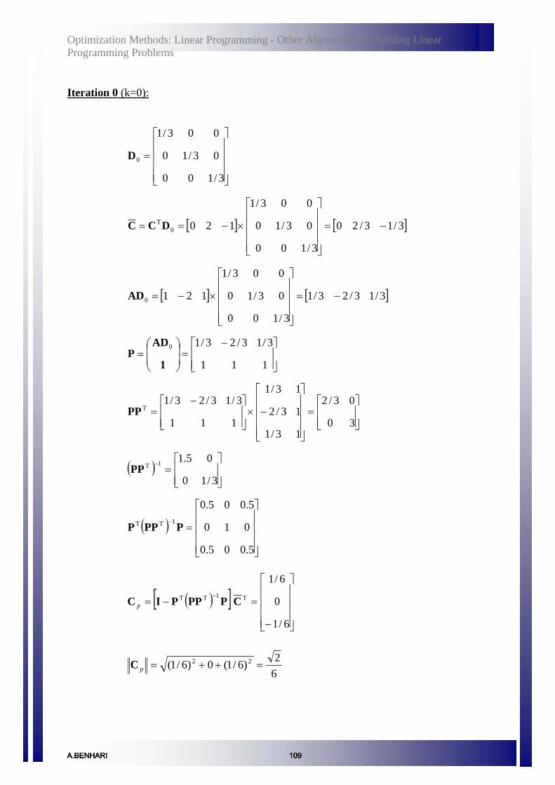
Optimization Methods: Linear Programming - Other Algorithms for Solving Linear Programming Problems
Iteration 0 (k=0):
⎥⎥⎥⎥
⎦
⎤
⎢⎢⎢⎢
⎣
⎡
=
3/100
03/10
003/1
0D
[ ] [ 3/13/20
3/100
03/10
003/1
1200T −=
⎥⎥⎥⎥
⎦
⎤
⎢⎢⎢⎢
⎣
⎡
×−== DCC ]
]
[ ] [ 3/13/23/1
3/100
03/10
003/1
1210 −=
⎥⎥⎥⎥
⎦
⎤
⎢⎢⎢⎢
⎣
⎡
×−=AD
⎥⎥⎦
⎤
⎢⎢⎣
⎡ −=⎟
⎟⎠
⎞⎜⎜⎝
⎛=
111
3/13/23/10
1
ADP
⎥⎥⎦
⎤
⎢⎢⎣
⎡=
⎥⎥⎥⎥
⎦
⎤
⎢⎢⎢⎢
⎣
⎡
−×⎥⎥⎦
⎤
⎢⎢⎣
⎡ −=
30
03/2
13/1
13/2
13/1
111
3/13/23/1TPP
( )⎥⎥⎦
⎤
⎢⎢⎣
⎡=
−
3/10
05.11TPP
( )⎥⎥⎥⎥
⎦
⎤
⎢⎢⎢⎢
⎣
⎡
=−
5.005.0
010
5.005.01TT PPPP
( )[ ]⎥⎥⎥⎥
⎦
⎤
⎢⎢⎢⎢
⎣
⎡
−
=−=−
6/1
0
6/1T1TT CPPPPIC p
62)6/1(0)6/1( 22 =++=pC
A.BENHARI 109A.BENHARI 109A.BENHARI 109

Optimization Methods: Linear Programming - Other Algorithms for Solving Linear Programming Problems
⎥⎥⎥⎥
⎦
⎤
⎢⎢⎢⎢
⎣
⎡
=
⎥⎥⎥⎥
⎦
⎤
⎢⎢⎢⎢
⎣
⎡
−
××
−
⎥⎥⎥⎥⎥⎥
⎦
⎤
⎢⎢⎢⎢⎢⎢
⎣
⎡
=−=
3974.0
3333.0
2692.0
6/1
0
6/1
62
61
92
31
31
31
0Mp
pnew r
C
CXY α
⎥⎥⎥⎥
⎦
⎤
⎢⎢⎢⎢
⎣
⎡
==
3974.0
3333.0
2692.0
1 newYX
[ ] 2692.0
3974.0
3333.0
2692.0
1201T =
⎥⎥⎥⎥
⎦
⎤
⎢⎢⎢⎢
⎣
⎡
×−== XCZ
Iteration 1 (k=1):
⎥⎥⎥⎥
⎦
⎤
⎢⎢⎢⎢
⎣
⎡
=
3974.000
03333.00
002692.0
1D
[ ] [T1
0.2692 0 0
0 2 1 0 0.3333 0 0 0.6667 0.3974
0 0 0.3974
⎡ ⎤⎢ ⎥⎢ ⎥= = − × = −⎢ ⎥⎢ ⎥⎣ ⎦
C C D ]
]
⎤
⎦
3
⎡ ⎤= ⎢ ⎥⎢ ⎥⎣ ⎦
[ ] [ 3974.06666.02692.03974.00003333.00002692.0
1211 −=⎥⎥⎥
⎦
⎤
⎢⎢⎢
⎣
⎡×−=AD
1 0.2692 0.6667 0.3974
1 1 1
−⎛ ⎞ ⎡= =⎜ ⎟ ⎢ ⎥⎜ ⎟ ⎢ ⎥⎝ ⎠ ⎣
ADP
1
T
0.2692 10.2692 0.6667 0.3974 0.675 0
0.6667 11 1 1 0
0.3974 1
⎡ ⎤− ⎢ ⎥⎡ ⎤
⎢ ⎥= × −⎢ ⎥⎢ ⎥⎢ ⎥⎣ ⎦⎢ ⎥⎣ ⎦
PP
( ) 1T1.482 0
0 0.333
− ⎡ ⎤= ⎢ ⎥⎢ ⎥⎣ ⎦
PP
A.BENHARI 110A.BENHARI 110A.BENHARI 110
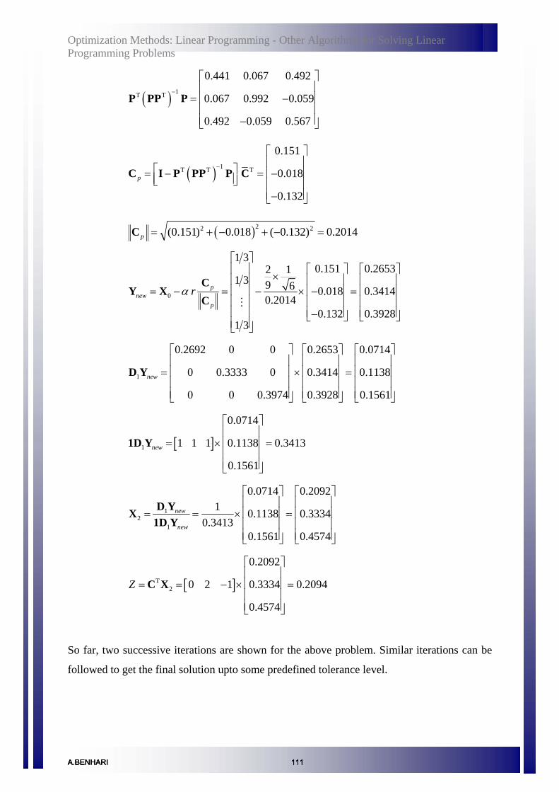
Optimization Methods: Linear Programming - Other Algorithms for Solving Linear Programming Problems
( ) 1T T
0.441 0.067 0.492
0.067 0.992 0.059
0.492 0.059 0.567
−
⎡ ⎤⎢ ⎥⎢ ⎥= −⎢ ⎥⎢ ⎥−⎣ ⎦
P PP P
( ) 1T T T
0.151
0.018
0.132
p
−
⎡ ⎤⎢ ⎥
⎡ ⎤ ⎢ ⎥= − = −⎢ ⎥⎣ ⎦ ⎢ ⎥⎢ ⎥−⎣ ⎦
C I P PP P C
( )22 2(0.151) 0.018 ( 0.132) 0.2014p = + − + − =C
0
1 30.151 0.26532 1
1 3 9 6 0.018 0.34140.2014
0.132 0.39281 3
pnew
p
rα
⎡ ⎤⎢ ⎥ ⎡ ⎤ ⎡ ⎤×⎢ ⎥ ⎢ ⎥ ⎢ ⎥⎢ ⎥ ⎢ ⎥ ⎢ ⎥= − = − × − =⎢ ⎥ ⎢ ⎥ ⎢ ⎥⎢ ⎥ ⎢ ⎥ ⎢ ⎥−⎣ ⎦ ⎣ ⎦⎢ ⎥⎣ ⎦
CY X
C M
1
0.2692 0 0 0.2653 0.0714
0 0.3333 0 0.3414 0.1138
0 0 0.3974 0.3928 0.1561
new
⎡ ⎤ ⎡ ⎤ ⎡ ⎤⎢ ⎥ ⎢ ⎥ ⎢ ⎥⎢ ⎥ ⎢ ⎥ ⎢ ⎥= × =⎢ ⎥ ⎢ ⎥ ⎢ ⎥⎢ ⎥ ⎢ ⎥ ⎢ ⎥⎣ ⎦ ⎣ ⎦ ⎣ ⎦
D Y
[ ]1
0.0714
1 1 1 0.1138 0.3413
0.1561
new
⎡ ⎤⎢ ⎥⎢ ⎥= × =⎢ ⎥⎢ ⎥⎣ ⎦
1D Y
12
1
0.0714 0.20921 0.1138 0.3334
0.34130.1561 0.4574
new
new
⎡ ⎤ ⎡ ⎤⎢ ⎥ ⎢ ⎥⎢ ⎥ ⎢ ⎥= = × =⎢ ⎥ ⎢ ⎥⎢ ⎥ ⎢ ⎥⎣ ⎦ ⎣ ⎦
D YX1D Y
[ ]T2
0.2092
0 2 1 0.3334 0.2094
0.4574
Z
⎡ ⎤⎢ ⎥⎢ ⎥= = − × =⎢ ⎥⎢ ⎥⎣ ⎦
C X
So far, two successive iterations are shown for the above problem. Similar iterations can be
followed to get the final solution upto some predefined tolerance level.
A.BENHARI 111A.BENHARI 111A.BENHARI 111

Optimization Methods: Linear Programming - Other Algorithms for Solving Linear Programming Problems
It may be noted that, the efficacy of Karmarkar’s projective scaling method is more
convincing for ‘large’ LP problems. Rigorous computational effort is not economical for
‘not-so-large’ problems.
A.BENHARI 112A.BENHARI 112A.BENHARI 112

Optimization Methods: Linear Programming Applications – Software
MATLAB Toolbox for Linear Programming
Optimization toolbox of MATLAB is very popular and efficient. It includes different types
of optimization techniques. In this lecture notes, we will briefly introduce the use of
MATLAB toolbox for Simplex Algorithm. However, it is assumed that the users are aware of
basics of MATLAB.
To use the simplex method, you have to set the option as 'LargeScale' to 'off' and 'Simplex' to
'on' in the following way.
options = optimset('LargeScale', 'off', 'Simplex', 'on')
Then a function called ‘linprog’ is to be used. A brief MATLAB documentation is shown in
Fig. 11 for linear programming (linprog).
A.BENHARIA.BENHARIA.BENHARI 113

Optimization Methods: Linear Programming Applications – Software
Fig. 11 MATLAB Documentation for Linear Programming
Further details may be referred from the toolbox. However, with this basic knowledge, simple
LP problems can be solved. Let us consider the same problem as considered earlier.
0,6
,52,532
21
21
21
1
21
≥≤+
−≥−≤+=
xxxxxx
xtoSubjectxxZMaximize
A.BENHARIA.BENHARIA.BENHARI 114
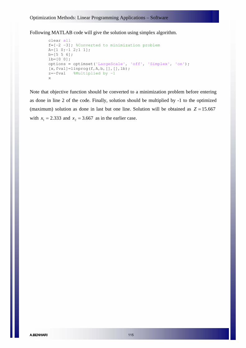
Optimization Methods: Linear Programming Applications – Software
Following MATLAB code will give the solution using simplex algorithm. clear all f=[-2 -3]; %Converted to minimization problem A=[1 0;-1 2;1 1]; b=[5 5 6]; lb=[0 0]; options = optimset('LargeScale', ff', 'Simplex', 'on'); 'o[x,fval]=linprog(f,A,b,[],[],lb); z=-fval %Multiplied by -1 x
Note that objective function should be converted to a minimization problem before entering
as done in line 2 of the code. Finally, solution should be multiplied by -1 to the optimized
(maximum) solution as done in last but one line. Solution will be obtained as
with and as in the earlier case.
667.15=Z
333.21 =x 667.32 =x
A.BENHARIA.BENHARIA.BENHARIA.BENHARI 115

Optimization Methods: Linear Programming Applications – Transportation Problem
Transportation Problem
Introduction
In the previous lectures, we discussed about the standard form of a LP and the commonly
used methods of solving LPP. A key problem in many projects is the allocation of scarce
resources among various activities. Transportation problem refers to a planning model that
allocates resources, machines, materials, capital etc. in a best possible way so that the costs
are minimized or profits are maximized. In this lecture, the common structure of a
transportation problem (TP) and its solution using LP are discussed followed by a numerical
example.
Structure of the Problem
The classic transportation problem is concerned with the distribution of any commodity
(resource) from any group of 'sources' to any group of destinations or 'sinks'. While solving
this problem using LP, the amount of resources from source to sink will be the decision
variables. The criterion for selecting the optimal values of the decision variables (like
minimization of costs or maximization of profits) will be the objective function. And the
limitation of resource availability from sources will constitute the constraint set.
Consider a general transportation problem consisting of m origins (sources) O1, O2,…, Om and
n destinations (sinks) D1, D2, … , Dn. Let the amount of commodity available in ith source be
ai (i=1,2,….m) and the demand in jth sink be bj (j=1,2,….n). Let the cost of transportation of
unit amount of material from i to j be cij. Let the amount of commodity supplied from i to j be
denoted as xij. Thus, the cost of transporting xij units of commodity from i to j is c . ijij x×
Now the objective of minimizing the total cost of transportation can be given as
Minimize (1) ∑∑= =
=m
i
n
jijij xcf
1 1
A.BENHARIA.BENHARIA.BENHARIA.BENHARI 116

Optimization Methods: Linear Programming Applications – Transportation Problem
Generally, in transportation problems, the amount of commodity available in a particular
source should be equal to the amount of commodity supplied from that source. Thus, the
constraint can be expressed as
∑ i= 1 ,2, … , m (2) =
=n
jiij ax
1,
Also, the total amount supplied to a particular sink should be equal to the corresponding
demand. Hence,
∑ j = 1 ,2, … , n (3) =
=m
ijij bx
1,
The set of constraints given by eqns (2) and (3) are consistent only if total supply and total
demand are equal.
∑ ∑= =
=m
i
n
jji ba
1 1
(4)
But in real problems this condition may not be satisfied. Then, the problem is said to be
unbalanced. However, the problem can be modified by adding a fictitious (dummy) source or
destination which will provide surplus supply or demand respectively. The transportation
costs from this dummy source to all destinations will be zero. Likewise, the transportation
costs from all sources to a dummy destination will be zero.
Thus, this restriction causes one of the constraints to be redundant. Thus the above problem
have m x n decision variables and (m + n - 1) equality constraints.
The non-negativity constraints can be expressed as
, i= 1 ,2, … , m , j = 1 ,2, … , n (5) 0≥ijx
This problem formulation is elucidated through an example given below.
A.BENHARIA.BENHARIA.BENHARI 117

Optimization Methods: Linear Programming Applications – Transportation Problem
Examples
Problem (1)
Consider a transport company which has to supply 4 units of paper materials from each of the
cities Faizabad and Lucknow to three cities. The material is to be supplied to Delhi,
Ghaziabad and Bhopal with demands of four, one and three units respectively. Cost of
transportation per unit of supply (cij) is indicated below in the figure. Decide the pattern of
transportation that minimizes the cost.
Solution:
Let the amount of material supplied from source i to sink j be xij. Here m =2; n = 3.
Total supply = 8 units and total demand = 4+1+3 = 8 units. Since both are equal, the problem
is balanced. The objective function is to minimize the total cost of transportation from all
combinations i.e.
Minimize ∑∑= =
=m
i
n
jijij xcf
1 1
A.BENHARIA.BENHARIA.BENHARI 118
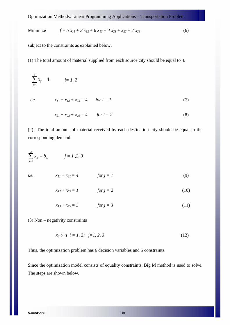
Optimization Methods: Linear Programming Applications – Transportation Problem
Minimize f = 5 x11 + 3 x12 + 8 x13 + 4 x21 + x22 + 7 x23 (6)
subject to the constraints as explained below:
(1) The total amount of material supplied from each source city should be equal to 4.
∑ i= 1, 2 =
=3
14
jijx
i.e. x11 + x12 + x13 = 4 for i = 1 (7)
x21 + x22 + x23 = 4 for i = 2 (8)
(2) The total amount of material received by each destination city should be equal to the
corresponding demand.
∑=
=2
1,
ijij bx j = 1 ,2, 3
i.e. x11 + x21 = 4 for j = 1 (9)
x12 + x22 = 1 for j = 2 (10)
x13 + x23 = 3 for j = 3 (11)
(3) Non – negativity constraints
xij 0≥ i = 1, 2; j=1, 2, 3 (12)
Thus, the optimization problem has 6 decision variables and 5 constraints.
Since the optimization model consists of equality constraints, Big M method is used to solve.
The steps are shown below.
A.BENHARIA.BENHARIA.BENHARI 119

Optimization Methods: Linear Programming Applications – Transportation Problem
Since there are five equality constraints, introduce five artificial variables R1, R2, R3, R4 and
R5. Thus, the objective function and the constraints can be expressed as
Minimize
54321
232221131211 714835RMRMRMRMRM
xxxxxxf×+×+×+×+×+×+×+×+×+×+×=
subject to
x11 + x12 + x13 + R1 = 4
x21 + x22 + x23 + R2 = 4
x11 + x21+ R3 = 4
x12+ x22 + R4 = 1
x13+ x23+ R5 = 3
Modifying the objective function to make the coefficients of the artificial variable equal to
zero, the final form objective function is
54321
232221
131211
00000)27()21()24()28()23()25(
RRRRRxMxMxMxMxMxMf
×+×+×+×+×−×+−+×+−+×+−+×+−+×+−+×+−+
The solution of the model using simplex method is shown
A.BENHARIA.BENHARIA.BENHARI 120

Optimization Methods: Linear Programming Applications – Transportation Problem
Table 1
First iteration
Variables Basic variables x11 x12 x13 x21 x22 x23 R1 R2 R3 R4 R5
RHS Ratio
Z -5 +2M
-3 +2M
-8 +2M
-4 +2M
-1 +2M
-7 +2M 0 0 0 0 0 16M
R1 1 1 1 0 0 0 1 0 0 0 0 4 -
R2 0 0 0 1 1 1 0 1 0 0 0 4 4
R31 0 0
1 0
0 0 0 1 0 0 4 -
R4 0 1 0 0 1 0 0 0 0 1 0 1 1
R5 0 0 1 0 0 1 0 0 0 0 1 3 -
Table 2
Second iteration
Variables Basic variables x11 x12 x13 x21 x22 x23 R1 R2 R3 R4 R5
RHS Ratio
Z -5+2M -1 -8+2M -4+2M 0 -7+2M 0 0 0 1-2M 0 1+14
M -
R1 1 1 1 0 0 0 1 0 0 0 0 4 -
R2 0 -1 0 1 0 0 0 1 0 -1 0 3 3
R3 1 0 0 1 0 0 0 0 1 0 0 4 4
X22 0 1 0 0 1 1 0 0 0 1 0 1 -
R5 0 0 1 0 0 1 0 0 0 0 1 3 -
A.BENHARIA.BENHARIA.BENHARI 121

Optimization Methods: Linear Programming Applications – Transportation Problem
Table 3
Third iteration
Variables Basic variables x11 x12 x13 x21 x22 x23 R1 R2 R3 R4 R5
RHS Ratio
Z -5+2M -5+2M -8+2M 0 0 -7+2M 0 4-2M 0 -3 0 13+8M -
R1 1 1 1 0 0 0 1 0 0 0 0 4 4
X21 0 -1 0 1 0 0 0 1 0 -1 0 3 -
R3 1 1 0 0 0 0 0 -1 1 1 0 1 1
X22 0 1 0 0 1 1 0 0 0 1 0 1 -
R5 0 0 1 0 0 1 0 0 0 0 1 3 -
Table 4
Fourth iteration
Variables Basic variables x11 x12 x13 x21 x22 x23 R1 R2 R3 R4 R5
RHS Ratio
Z 0 0 -8+2M 0 0 -7+2M 0 -1 5-2M
2-2M 0 18+6M -
R1 0 0 1 0 0 0 1 1 -1 -1 0 3 -
X21 0 -1 0 1 0 0 0 1 0 -1 0 3 -
X11 1 1 0 0 0 0 0 -1 1 1 0 1 -
X22 0 1 0 0 1 1 0 0 0 1 0 1 1
R5 0 0 1 0 0 1 0 0 0 0 1 3 3
Repeating the same procedure, we get the final optimal solution f = 42 and the optimum
decision variable values as : x11 = 2.2430, x12 = 0.00, x13 = 1.7570, x21 = 1.7570, x22 =
1.00, x23 = 1.2430.
A.BENHARIA.BENHARIA.BENHARI 122

Optimization Methods: Linear Programming Applications – Transportation Problem
Problem (2)
Consider three factories (F) located in three different cities, producing a particular chemical.
The chemical is to be transported to four different warehouses (Wh), from where it is
supplied to the customers. The transportation cost per truck load from each factory to each
warehouse is determined and are given in the table below. Production and demands are also
given in the table below.
Wh1 Wh2 Wh3 Wh4 Production
F1 523 682 458 850 60
F2 420 412 362 729 110
F3 670 558 895 695 150
Demand 65 85 80 70
Solution:
Let the amount of chemical to be transported from factory i to warehouse j be xij.
Total supply = 60+110+150 = 320 and total demand = 65+85+80+70 = 300. Since the total
demand is less than total supply, add one fictitious ware house, Wh5 with a demand of 20.
Thus, here m =3; n = 5
Wh1 Wh2 Wh3 Wh4 Wh5 Production
F1 523 682 458 850 0 60
F2 420 412 362 729 0 110
F3 670 558 895 695 0 150
Demand 65 85 80 70 20
The objective function is to minimize the total cost of transportation from all combinations.
Minimize f = 523 x11 + 682 x12 + 458 x13+ 850 x14 + 0 x15 + 420 x21 + 412 x22 + 362 x23
+ 729 x24 + 0 x25 + 670 x31 + 558 x32 + 895 x33 +695 x34 + 0 x35
subject to the constraints
A.BENHARIA.BENHARIA.BENHARI 123

Optimization Methods: Linear Programming Applications – Transportation Problem
x11 + x12 + x13 + x14+ x15 = 60 for i = 1
x21 + x22 + x23 + x24+ x25 = 110 for i = 2
x31 + x32 + x33 + x34 + x35 = 150 for i = 3
x11 + x21+ x31 = 65 for j = 1
x12 + x22+ x32 = 85 for j = 2
x13 + x23 + x23 =90 for j = 3
x14 + x24 + x24 =80 for j = 4
x15 + x25 + x25 =20 for j = 5
xij 0≥ i = 1, 2,3; j=1, 2, 3,4
This optimization problem can be solved using the same procedure used for the previous
problem.
A.BENHARIA.BENHARIA.BENHARI 124

Optimization Methods: Linear Programming Applications – Assignment Problem
Assignment Problem
Introduction
In the previous lecture, we discussed about one of the bench mark problems called
transportation problem and its formulation. The assignment problem is a particular class of
transportation linear programming problems with the supplies and demands equal to
integers (often 1). Since all supplies, demands, and bounds on variables are integers, the
assignment problem relies on an interesting property of transportation problems that the
optimal solution will be entirely integers. In this lecture, the structure and formulation of
assignment problem are discussed. Also, traveling salesman problem, which is a special
type of assignment problem, is described.
Structure of assignment problem
As mentioned earlier, assignment problem is a special type of transportation problem in
which
1. Number of supply and demand nodes are equal.
2. Supply from every supply node is one.
3. Every demand node has a demand of one.
4. Solution is required to be all integers.
The goal of a general assignment problem is to find an optimal assignment of machines
(laborers) to jobs without assigning an agent more than once and ensuring that all jobs are
completed. The objective might be to minimize the total time to complete a set of jobs, or
to maximize skill ratings, maximize the total satisfaction of the group or to minimize the
cost of the assignments. This is subjected to the following requirements:
A.BENHARIA.BENHARIA.BENHARIA.BENHARI 125

Optimization Methods: Linear Programming Applications – Assignment Problem
1. Each machine is assigned not more than one job.
2. Each job is assigned to exactly one machine.
Formulation of assignment problem
Consider m laborers to whom n tasks are assigned. No laborer can either sit idle or do
more than one task. Every pair of person and assigned work has a rating. This rating may
be cost, satisfaction, penalty involved or time taken to finish the job. There will be N2 such
combinations of persons and jobs assigned. Thus, the optimization problem is to find such
man- job combinations that optimize the sum of ratings among all.
The formulation of this problem as a special case of transportation problem can be
represented by treating laborers as sources and the tasks as destinations. The supply
available at each source is 1 and the demand required at each destination is 1.The cost of
assigning (transporting) laborer i to task j is cij.
It is necessary to first balance this problem by adding a dummy laborer or task depending
on whether m<n or m>n, respectively. The cost coefficient cij for this dummy will be zero.
Let ⎪⎩
⎪⎨⎧
=machineithetoassignedisjobjtheif
machineithetoassignednotisjobjtheifx
thth
thth
ij ,1,0
Thus the above model can be expressed as
∑∑= =
m
i
n
jijij xcMinimize
1 1
Since each task is assigned to exactly one laborer and each laborer is assigned only one
job, the constraints are
A.BENHARIA.BENHARIA.BENHARI 126

Optimization Methods: Linear Programming Applications – Assignment Problem
1
1
1 1,2,...
1 1,2,...
n
ijin
ijj
x for j n
x for i m
=
=
= =
= =
∑
∑
10 orxij =
Due to the special structure of the assignment problem, the solution can be found out using
a more convenient method called Hungarian method which will be illustrated through an
example below.
Example 1: (Taha, 1982)
Consider three jobs to be assigned to three machines. The cost for each combination is
shown in the table below. Determine the minimal job – machine combinations.
Table 1
Machine Job
1 2 3 ai
1 5 7 9 1
2 14 10 12 1
3 15 13 16 1
bj 1 1 1
Solution:
Step 1:
Create zero elements in the cost matrix (zero assignment) by subtracting the smallest
element in each row (column) from the corresponding row (column). After this exercise,
the resulting cost matrix is obtained by subtracting 5 from row 1, 10 from row 2 and 13
from row 3.
A.BENHARIA.BENHARIA.BENHARI 127

Optimization Methods: Linear Programming Applications – Assignment Problem
Table 2
1 2 3
1 0 2 4
2 4 0 2
3 2 0 3
Step 2:
Repeating the same with columns, the final cost matrix is
Table 3
1 2 3
1 0 2 2
2 4 0 0
3 2 0 3
The italicized zero elements represent a feasible solution. Thus the optimal assignment is
(1,1), (2,3) and (3,2). The total cost is equal to 60 (5 +12+13).
In the above example, it was possible to obtain the feasible assignment. But in more
complicated problems, additional rules are required which are explained in the next
example.
Example 2 (Taha, 1982)
Consider four jobs to be assigned to four machines. The cost for each combination is
shown in the table below. Determine the minimal job – machine combinations.
A.BENHARIA.BENHARIA.BENHARI 128
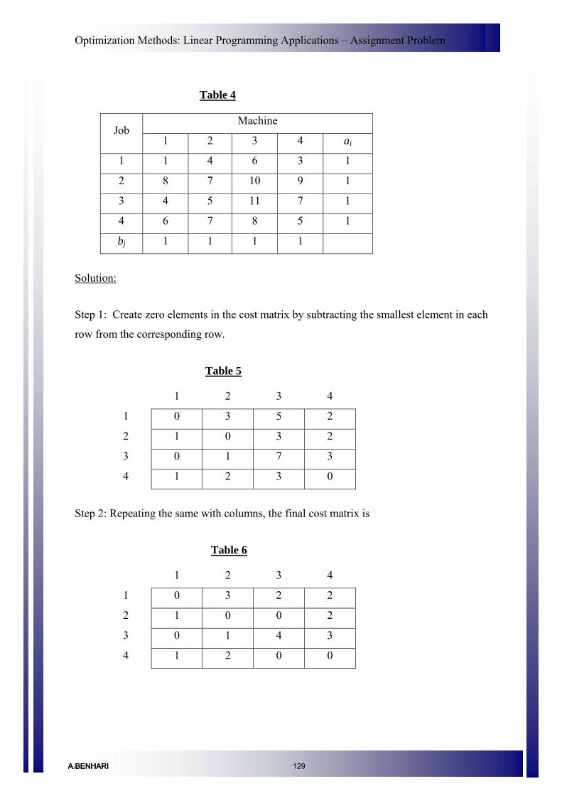
Optimization Methods: Linear Programming Applications – Assignment Problem
Table 4
Machine Job
1 2 3 4 ai
1 1 4 6 3 1
2 8 7 10 9 1
3 4 5 11 7 1
4 6 7 8 5 1
bj 1 1 1 1
Solution:
Step 1: Create zero elements in the cost matrix by subtracting the smallest element in each
row from the corresponding row.
Table 5
1 2 3 4
1 0 3 5 2
2 1 0 3 2
3 0 1 7 3
4 1 2 3 0
Step 2: Repeating the same with columns, the final cost matrix is
Table 6
1 2 3 4
1 0 3 2 2
2 1 0 0 2
3 0 1 4 3
4 1 2 0 0
A.BENHARIA.BENHARIA.BENHARI 129
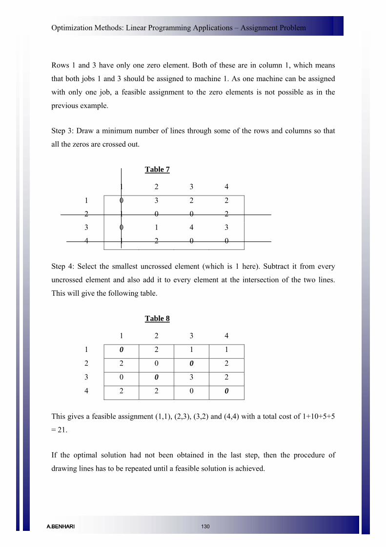
Optimization Methods: Linear Programming Applications – Assignment Problem
Rows 1 and 3 have only one zero element. Both of these are in column 1, which means
that both jobs 1 and 3 should be assigned to machine 1. As one machine can be assigned
with only one job, a feasible assignment to the zero elements is not possible as in the
previous example.
Step 3: Draw a minimum number of lines through some of the rows and columns so that
all the zeros are crossed out.
Table 7
1 2 3 4
1 0 3 2 2
2 1 0 0 2
3 0 1 4 3
4 1 2 0 0
Step 4: Select the smallest uncrossed element (which is 1 here). Subtract it from every
uncrossed element and also add it to every element at the intersection of the two lines.
This will give the following table.
Table 8
1 2 3 4
1 0 2 1 1
2 2 0 0 2
3 0 0 3 2
4 2 2 0 0
This gives a feasible assignment (1,1), (2,3), (3,2) and (4,4) with a total cost of 1+10+5+5
= 21.
If the optimal solution had not been obtained in the last step, then the procedure of
drawing lines has to be repeated until a feasible solution is achieved.
A.BENHARIA.BENHARIA.BENHARI 130

Optimization Methods: Linear Programming Applications – Assignment Problem
Formulation of Traveling Salesman Problem (TSP) as an Assignment Problem
A traveling salesman has to visit n cities and return to the starting point. He has to start
from any one city and visit each city only once. Suppose he starts from the kth city and the
last city he visited is m. Let the cost of travel from ith city to jth city be cij. Then the
objective function is
∑∑= =
m
i
n
jijij xcMinimize
1 1
subject to the constraints
1
1
1 1,2,... , ,
1 1,2,... , ,
10 1
n
ijin
ijj
mk
ij
x for j n i j i m
x for i m i j i m
xx or
=
=
= = ≠
= = ≠
==
∑
∑
≠
≠
Solution Procedure:
Solve the problem as an assignment problem using the method used to solve the above
examples. If the solutions thus found out are cyclic in nature, then that is the final solution.
If it is not cyclic, then select the lowest entry in the table (other than zero). Delete the row
and column of this lowest entry and again do the zero assignment in the remaining matrix.
Check whether cyclic assignment is available. If not, include the next higher entry in the
table and the procedure is repeated until a cyclic assignment is obtained.
The procedure is explained through an example below.
A.BENHARIA.BENHARIA.BENHARI 131

Optimization Methods: Linear Programming Applications – Assignment Problem
Example 3:
Consider a four city TSP for which the cost between the city pairs are as shown in the
figure below. Find the tour of the salesman so that the cost of travel is minimal.
2
6 8 4
5 1 4
9 9
3
Table 9
1 2 3 4
1 ∞ 4 9 5
2 6 ∞ 4 8
3 9 4 ∞ 9
4 5 8 9 ∞
Solution:
Step 1: The optimal solution after using the Hungarian method is shown below.
Table 10
1 2 3 4
1 ∞ 0 5 0
2 2 ∞ 0 3
3 5 0 ∞ 4
4 0 3 4 ∞
A.BENHARIA.BENHARIA.BENHARI 132
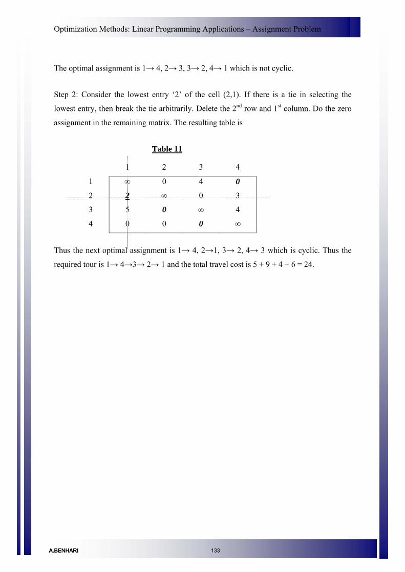
Optimization Methods: Linear Programming Applications – Assignment Problem
The optimal assignment is 1→ 4, 2→ 3, 3→ 2, 4→ 1 which is not cyclic.
Step 2: Consider the lowest entry ‘2’ of the cell (2,1). If there is a tie in selecting the
lowest entry, then break the tie arbitrarily. Delete the 2nd row and 1st column. Do the zero
assignment in the remaining matrix. The resulting table is
Table 11
1 2 3 4
1 ∞ 0 4 0
2 2 ∞ 0 3
3 5 0 ∞ 4
4 0 0 0 ∞
Thus the next optimal assignment is 1→ 4, 2→1, 3→ 2, 4→ 3 which is cyclic. Thus the
required tour is 1→ 4→3→ 2→ 1 and the total travel cost is 5 + 9 + 4 + 6 = 24.
A.BENHARIA.BENHARIA.BENHARI 133

Optimization Methods: Linear Programming Applications – Structural & Water Resources Problems
Structural & Water Resources Problems
Introduction
In the previous lectures, some of the bench mark problems which use LP were discussed. LP
has been applied to formulate and solve several types of problems in engineering field also.
LP finds many applications in the field of water resources and structural design which include
many types like planning of urban water distribution, reservoir operation, crop water
allocation, minimizing the cost and amount of materials in structural design. In this lecture,
applications of LP in the plastic design of frame structures and also in deciding the optimal
irrigation allocation and water quality management are discussed.
Typical Example – Structural Design
(1) A beam column arrangement of a rigid frame is shown below. Moment in beam is
represented by Mb and moment in column is denoted by Mc. l = 8 units and h= 6 units and
forces F1=2 units and F2=1 unit. Assuming that plastic moment capacity of beam and
columns are linear functions of their weights; the objective function is to minimize the sum of
weights of the beam and column materials.
Fig. 1
F2=1
F1=2 3 4 52 6
h=6
1 7l=8l=8
A.BENHARIA.BENHARIA.BENHARIA.BENHARI 134

Optimization Methods: Linear Programming Applications – Structural & Water Resources Problems
Solution:
In the plastic limit design, it is assumed that at the points of peak moments, plastic hinges
will be developed. The points of development of peak moments are numbered in the above
figure from 1 through 7. The development of sufficient hinges makes the structure unstable
known as a collapse mechanism. Thus, for the design to be safe the energy absorbing
capacity of the frame (U) should be greater than the energy imparted by externally applied
load (E) for the various collapse mechanisms of the structure.
The objective function can be written as
Minimize f = weight of beam + weight of column
i.e. (2 2b )cf w lM hM= + (1)
where w is weight per unit length over unit moment in material. Since w is constant,
optimizing (1) is same as optimizing
( )2 216 12
b
b c
cf lM hMM M
= +
= + (2)
The four possible collapse mechanisms are shown in the figure below with the corresponding
U and E values. Constraints are formulated from the design restriction U for all the
mechanisms.
E≥
(a) (b)
A.BENHARIA.BENHARIA.BENHARI 135
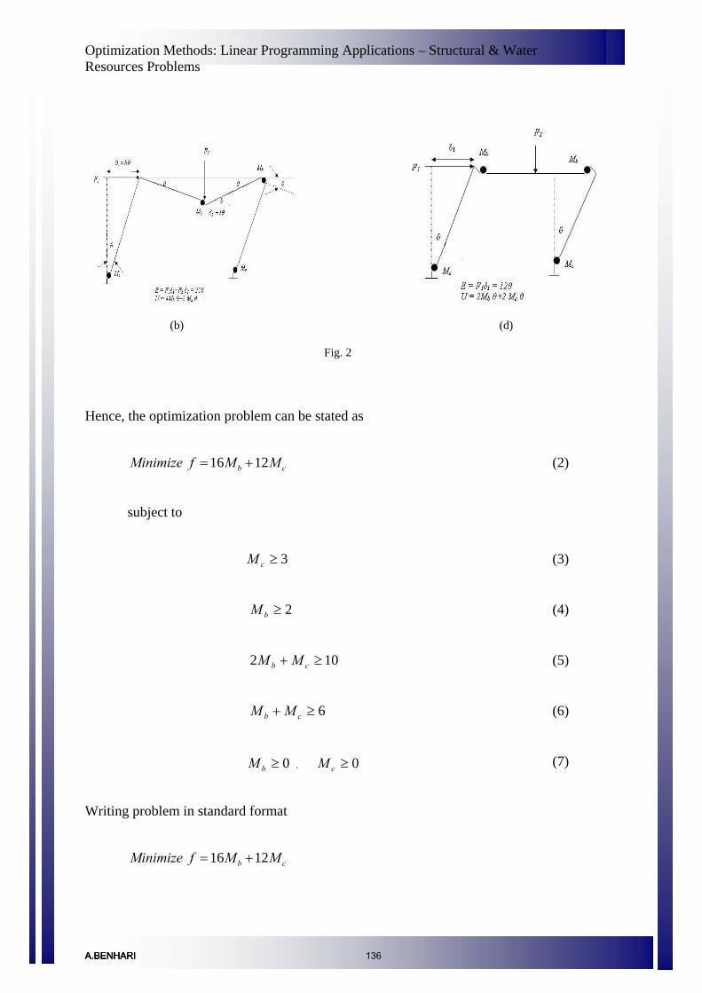
Optimization Methods: Linear Programming Applications – Structural & Water Resources Problems
(b) (d) Fig. 2
Hence, the optimization problem can be stated as
16 12b cMinimize f M M= + (2)
subject to
(3) 3≥cM
(4) 2≥bM
(5) 102 ≥+ cb MM
(6) 6≥+ cb MM
, 0≥bM 0≥cM (7)
Writing problem in standard format
16 12b cMinimize f M M= +
A.BENHARIA.BENHARIA.BENHARI 136
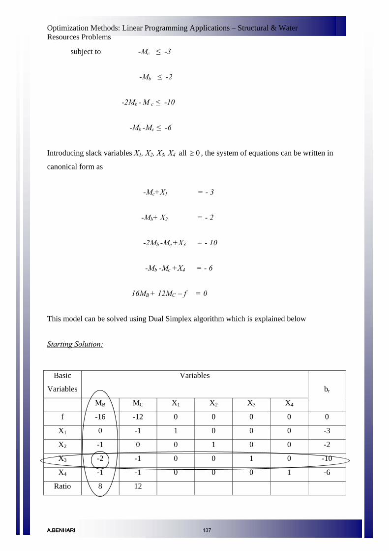
Optimization Methods: Linear Programming Applications – Structural & Water Resources Problems
subject to -Mc ≤ -3
-Mb ≤ -2
-2Mb - M c ≤ -10
-Mb -Mc ≤ -6
Introducing slack variables X1, X2, X3, X4 all , the system of equations can be written in
canonical form as
0≥
-Mc+X1 = - 3
-Mb+ X2 = - 2
-2Mb -Mc +X3 = - 10
-Mb -Mc +X4 = - 6
16MB + 12MC – f = 0
This model can be solved using Dual Simplex algorithm which is explained below
Starting Solution:
Basic
Variables
Variables
MB MC X1 X2 X3 X4
br
f -16 -12 0 0 0 0 0
X1 0 -1 1 0 0 0 -3
X2 -1 0 0 1 0 0 -2
X3 -2 -1 0 0 1 0 -10
X4 -1 -1 0 0 0 1 -6
Ratio 8 12
A.BENHARIA.BENHARIA.BENHARI 137

Optimization Methods: Linear Programming Applications – Structural & Water Resources Problems
Iteration 1:
Basic
Variables Variables
MB MC X1 X2 X3 X4
br
f 0 -4 0 0 -8 0 80
X1 0 -1 1 0 0 0 -3
X2 0 ½ 0 1 -½ 0 3
MB 1 ½ 0 0 -½ 0 5
X4 0 -½ 0 0 -½ 1 -1
Ratio 4
Iteration 2:
Basic
Variables Variables
MB MC X1 X2 X3 X4
br
f 0 0 -4 0 -8 0 92
MC 0 1 -1 0 0 0 3
X2 0 0 ½ 1 -½ 0 3/2
MB 1 0 ½ 0 -½ 0 7/2
X4 0 0 -½ 0 -½ 1 1
Ratio
The optimal value of decision variables are
MB =7/2; MC =3
And the total weight of the material required f = 92w units.
A.BENHARIA.BENHARIA.BENHARI 138
Optimization Methods: Linear Programming Applications – Structural & Water Resources Problems
Typical Example – Water Resources
(2) Consider two crops 1 and 2. One unit of crop 1 produces four units of profit and one
unit of crop 2 brings five units of profit. The demand of production of crop 1 is A units and
that of crop 2 is B units. Let x be the amount of water required for A units of crop 1 and y be
the same for B units of crop 2. The amount of production and the amount of water required
can be expressed as a linear relation as shown below
A = 0.5(x - 2) + 2
B = 0.6(y - 3) + 3
Minimum amount of water that must be provided to 1 and 2 to meet their demand is two and
three units respectively. Maximum availability of water is ten units. Find out the optimum
pattern of irrigation.
Solution:
The objective is to maximize the profit from crop 1 and 2, which can be represented as
Maximize f = 4A + 5B;
Expressing as a function of the amount of water,
Maximize f = 4[0.5(x - 2) + 2] + 5[0.6(y - 3) + 3]= 2x + 3y + 10
subject to
; Maximum availability of water 10≤+ yx
; Minimum amount of water required for crop 1 2≥x
; Minimum amount of water required for crop 2 3≥y
The above problem is same as maximizing f’ = 2x + 3y subject to same constraints.
A.BENHARIA.BENHARIA.BENHARI 139

Optimization Methods: Linear Programming Applications – Structural & Water Resources Problems
Changing the problem into standard form by introducing slack variables S1, S2, S3
Maximize f’ = 2x + 3y
subject to
x + y + S1 =10
-x + S2 = -2
-y + S3 = -3
This model is solved by forming the simplex table as below
Starting Solution:
Variables Basic Variables x y S1 S2 S3
RHS Ratio
f’ -2 -3 0 0 0 0
S1 1 1 1 0 0 10 10
S2 -1 0 0 1 0 -2 -
S3 0 -1 0 0 1 -3 3
A.BENHARIA.BENHARIA.BENHARI 140

Optimization Methods: Linear Programming Applications – Structural & Water Resources Problems
Iteration 1:
Variables Basic Variables x y S1 S2 S3
RHS Ratio
f’ -2 0 0 0 -3 9 -
S1 1 0 1 0 1 7 7
S2 -1 0 0 1 0 -2 2
y 0 1 0 0 -1 3 -
Iteration 2:
Variables Basic Variables x y S1 S2 S3
RHS Ratio
f’ 0 0 0 -2 -3 13 -
S1 0 0 1 1 1 5 5
x 1 0 0 -1 0 2 -
y 0 1 0 0 -1 3 -3
Iteration 3:
Variables Basic Variables x y S1 S2 S3
RHS Ratio
f’ 0 0 3 1 0 28 -
S3 0 0 1 1 1 5 -
x 1 0 0 -1 0 2 -
y 0 1 1 1 0 8 -
A.BENHARIA.BENHARIA.BENHARI 141
Optimization Methods: Linear Programming Applications – Structural & Water Resources Problems
Hence the solution is
x = 2; y = 8; f’ = 28
Therefore, f = 28+10 = 38
Thus, water allocated to crop A is 2 units and to crop B is 8 units and total profit yielded is 38
units.
Typical Example – Water Quality Management
Waste load allocation for water quality management in a river system can be defined as
determination of optimal treatment level of waste, which is discharged to a river; such that
the water quality standards set by Pollution Control Agency (PCA) are maintained through
out the river. Conventional waste load allocation involves minimization of treatment cost
subject to the constraint that the water quality standards are not violated.
Consider a simple problem, where, there are M dischargers, who discharge waste into the
river, and I checkpoints, where the water quality is measured by PCA. Let xj is the treatment
level and aj is the unit treatment cost for jth discharger (j=1,2,…,M). ci is the dissolved oxygen
(DO) concentration at checkpoint i (i=1,2,…,I), which is to be controlled. Therefore the
decision variables for the waste load allocation model are xj (j=1,2,…,M).
Thus, the objective function can be expressed as
1
M
j jj
Maximize f a x=
=∑
The relationship between the water quality indicator, ci (DO) at a checkpoint and the
treatment level upstream to that checkpoint is linear (based on Streeter-Phelps Equation)
when all other parameters involved in water quality simulations are constant. Let g(x) denotes
the linear relationship between ci and xj. Then,
( ) ,i jc g x i= ∀ j
A.BENHARIA.BENHARIA.BENHARI 142

Optimization Methods: Linear Programming Applications – Structural & Water Resources Problems
Let cP be the permissible DO level set by PCA, which is to be maintained through out the
river. Therefore,
i Pc c≥ ∀i
Solution of the optimization model using simplex algorithm gives the optimal fractional
removal levels required to maintain the water quality of the river.
A.BENHARIA.BENHARIA.BENHARI 143
Optimization Methods: Dynamic Programming - Introduction
Introduction
Introduction
In some complex problems, it will be advisable to approach the problem in a sequential
manner in order to find the solution quickly. The solution is found out in multi stages. This is
the basic approach behind dynamic programming. It works in a “divide and conquer”
manner. The word "programming" in "dynamic programming" has no particular connection
to computer programming at all. A program is, instead, the plan for action that is produced. In
this lecture, the multistage decision process, its representation, various types and the concept
of sub-optimization and principle of optimality are discussed.
Sequential optimization
In sequential optimization, a problem is approached by dividing it into smaller subproblems
and optimization is done for these subproblems without losing the integrity of the original
problem. Sequential decision problems are those in which decisions are made in multiple
stages. These are also called multistage decision problems since decisions are made at a
number of stages.
In multistage decision problems, an N variable problem is represented by N single variable
problems. These problems are solved successively such that the optimal value of the original
problem can be obtained from the optimal solutions of these N single variable problems. The
N single variable problems are connected in series so that the output of one stage will be the
input to the succeeding stage. This type of problem is called serial multistage decision
process.
For example, consider a water allocation problem to N users. The objective function is to
maximize the total net benefit from all users. This problem can be solved by considering each
user separately and optimizing the individual net benefits, subject to constraints and then
adding up the benefits from all users to get the total optimal benefit.
A.BENHARIA.BENHARIA.BENHARIA.BENHARI 144
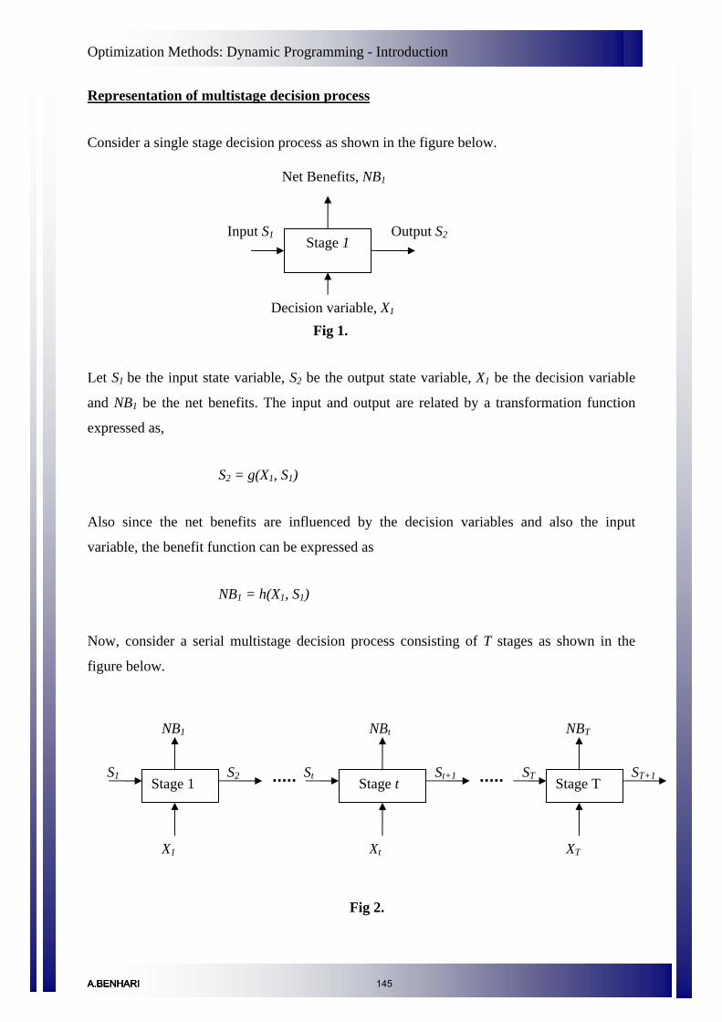
Optimization Methods: Dynamic Programming - Introduction
Representation of multistage decision process
Consider a single stage decision process as shown in the figure below.
Net Benefits, NB1
Stage 1 Input S1 Output S2
Decision variable, X1 Fig 1.
Let S1 be the input state variable, S2 be the output state variable, X1 be the decision variable
and NB1 be the net benefits. The input and output are related by a transformation function
expressed as,
S2 = g(X1, S1)
Also since the net benefits are influenced by the decision variables and also the input
variable, the benefit function can be expressed as
NB1 = h(X1, S1)
Now, consider a serial multistage decision process consisting of T stages as shown in the
figure below.
Stage 1 Stage t Stage T St
NBt
Xt
St+1 S1 S2
NB1 NBT
X1 XT
ST ST+1
Fig 2.
A.BENHARIA.BENHARIA.BENHARI 145

Optimization Methods: Dynamic Programming - Introduction
Here, for the tth stage the, state transformation and the benefit functions are written as,
St+1 = g(Xt, St)
NBt = h(Xt, St)
The objective of this multistage problem is to find the optimum values of all decision
variables X1, X2,…, XT such that the individual net benefits of each stage that is expressed by
some objective function, f(NBt) and the total net benefit which is expressed by f(NB1,
NB2,…, NBT) should be maximized. The application of dynamic programming to a multistage
problem depends on the nature of this objective function i.e., the objective function should be
separable and monotonic. An objective function is separable, if it can be decomposed and
expressed as a sum or product of individual net benefits of each stage, i.e.,
either ( )∑ ∑= =
==T
t
T
tttt SXhNBf
1 1,
or ( )∏∏==
==T
ttt
T
tt SXhNBf
11
,
An objective function is monotonic if for all values of a and b for which the value of the
benefit function is ( ) ( )tttt SbxhSaxh ,, =≥= , then
( ) ( )1,211,21 ,,...,...,,,,...,...,, ++ =≥= tTttTt SxbxxxfSxaxxxf
should be satisfied.
A.BENHARIA.BENHARIA.BENHARI 146

Optimization Methods: Dynamic Programming - Introduction
Types of multistage decision problems
A serial multistage problem such as shown, can be classified into three categories as initial
value problem, final value problem and boundary value problem.
1. Initial value problem: In this type, the value of the initial state variable, S1 is given.
2. Final value problem: In this, the value of the final state variable, ST is given. A final
value problem can be transformed into an initial value problem by reversing the
procedure of computation of the state variable, St.
3. Boundary value problem: In this, the values of both the initial and final state
variables, S1 and ST are given.
Concept of sub-optimization and principle of optimality
Bellman (1957) stated the principle of optimality which explains the process of suboptimality
as:
“An optimal policy (or a set of decisions) has the property that whatever the initial state and
initial decision are, the remaining decisions must constitute an optimal policy with regard to
the state resulting from the first decision.”
Consider the objective function consisting of T decision variables x1, x2, …, xT,
( )∑ ∑= =
==T
t
T
tttt SXhNBf
1 1,
and satisfying the equations,
St+1 = g(Xt, St)
NBt = h(Xt, St) for t = 1,2,…,T
The concepts of suboptimization and principle of optimality are used to solve this problem
through dynamic programming. To explain these concepts, consider the design of a water
tank in which the cost of construction is to be minimized. The capacity of the tank to be
designed is given as K.
A.BENHARIA.BENHARIA.BENHARI 147

Optimization Methods: Dynamic Programming - Introduction
The main components of a water tank include (i) tank (ii) columns to support the tank and
(iii) the foundation. While optimizing this problem to minimize the cost, it would be
advisable to break this system into individual parts and optimizing each part separately
instead of considering the system as a whole together. However, while breaking and doing
suboptimization, a logical procedure should be used; otherwise this approach can lead to a
poor solution. For example, consider the suboptimization of columns without considering the
other two components. In order to reduce the construction cost of columns, one may use
heavy concrete columns with less reinforcement, since the cost of steel is high. But while
considering the suboptimization of foundation component, the cost becomes higher as the
foundation should be strong enough to carry these heavy columns. Thus, the suboptimization
of columns before considering the suboptimization of foundation will adversely affect the
overall design.
In most of the serial systems as discussed above, since the suboptimization of last component
does not influence the other components, it can be suboptimized independently. For the
above problem, foundation can thus be suboptimized independently. Then the last two
components (columns and foundation) are considered as a single component and
suboptimization is done without affecting other components. This process can be repeated for
any number of end components. The process of suboptimization for the above problem is
shown in the next page.
A.BENHARIA.BENHARIA.BENHARI 148

Optimization Methods: Dynamic Programming - Introduction
Tank Columns Foundation
Original System
Tank Columns Foundation
Suboptimize design of Foundation component
Fig 3.
Tank Columns Foundation
Tank Columns Foundation
Suboptimize design of Foundation & Columns together
Optimize complete system
A.BENHARIA.BENHARIA.BENHARI 149
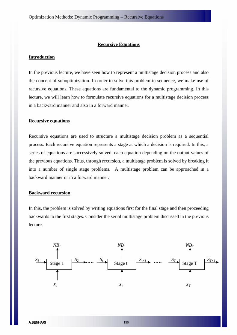
Optimization Methods: Dynamic Programming – Recursive Equations
Recursive Equations
Introduction
In the previous lecture, we have seen how to represent a multistage decision process and also
the concept of suboptimization. In order to solve this problem in sequence, we make use of
recursive equations. These equations are fundamental to the dynamic programming. In this
lecture, we will learn how to formulate recursive equations for a multistage decision process
in a backward manner and also in a forward manner.
Recursive equations
Recursive equations are used to structure a multistage decision problem as a sequential
process. Each recursive equation represents a stage at which a decision is required. In this, a
series of equations are successively solved, each equation depending on the output values of
the previous equations. Thus, through recursion, a multistage problem is solved by breaking it
into a number of single stage problems. A multistage problem can be approached in a
backward manner or in a forward manner.
Backward recursion
In this, the problem is solved by writing equations first for the final stage and then proceeding
backwards to the first stages. Consider the serial multistage problem discussed in the previous
lecture.
Stage 1 Stage t Stage T St
NBt
Xt
S1 S2
NB1 NBT
X1 XT
ST ST+1 St+1
A.BENHARIA.BENHARIA.BENHARIA.BENHARI 150

Optimization Methods: Dynamic Programming – Recursive Equations
Suppose the objective function for this problem is
( )
( ) ( ) ( ) ( ) ( ) )1...(,,...,...,,
,
111222111
1 1
TTTTTTttt
T
t
T
ttttt
SXhSXhSXhSXhSXh
SXhNBf
++++++=
==
−−−
= =∑ ∑
and the relation between the stage variables and decision variables are gives as
St+1 = g(Xt, St), t = 1,2,…, T. …(2)
Consider the final stage as the first subproblem. The input variable to this stage is ST.
According to the principle of optimality, no matter what happens in other stages, the decision
variable XT should be selected such that ( )TTT SXh ,∗
Tf
is optimum for the input ST. Let the
optimum value be denoted as . Then,
( )[ ] )3...(,)( TTTX
TT SXhoptSfT
=∗
Next, group the last two stages together as the second subproblem. Let be the optimum
objective value of this subproblem. Then, we have
∗−1Tf
( ) ( )[ ] )4...(,,)( 111,
111
TTTTTTXX
TT SXhSXhoptSfTT
+= −−−−∗−
−
From the principle of optimality, the value of should be to optimize for a given .
For obtaining , we need and . Thus, can be written as,
TX Th TS
TS 1−TS 1−TX )( 11 −∗− TT Sf
( )[ ] )5...()(,)( 111111
TTTTTX
TT SfSXhoptSfT
∗−−−−
∗− +=
−
By using the stage transformation equation, can be rewritten as, )( 11 −∗− TT Sf
( ) ( )( )[ ] )6...(,,)( 111111111
−−−∗
−−−−∗− +=
−
TTTTTTTX
TT SXgfSXhoptSfT
A.BENHARIA.BENHARIA.BENHARI 151
Optimization Methods: Dynamic Programming – Recursive Equations
Thus, here the optimum is determined by choosing the decision variable for a given
input . Eqn (4) which is a multivariate problem (second sub problem) is divided into two
single variable problems as shown in eqns (3) and (6). In general, the i+1
1−TX
1−TSth subproblem (T-ith
stage) can be expressed as,
( ) ( ) ( )[ ] )7...(,,...,)( 111,,..., 1
TTTTTTiTiTiTXXX
iTiT SXhSXhSXhoptSfTTiT
+++= −−−−−−−∗−
−−
Converting this to a single variable problem,
( ) ( )( )[ ] )8...(,,)( )1( iTiTiTiTiTiTiTX
iTiT SXgfSXhoptSfiT
−−−∗
−−−−−−∗− +=
−
where denotes the optimal value of the objective function for the last i stages. Thus
for backward recursion, the principle of optimality can be stated as, no matter in what state of
stage one may be, in order for a policy to be optimal, one must proceed from that state and
stage in an optimal manner.
∗−− )1(iTf
Forward recursion
In this approach, the problem is solved by starting from the stage 1 and proceeding towards
the last stage. Consider the serial multistage problem with the objective function as given
below
( )
T T
( ) ( ) ( ) ( ) ( ) )9...(,,...,...,,
,
111222111
1 1
TTTTTTttt
t ttttt
SXhSXhSXhSXhSXh
SXhNBf
++++++=
==
−−−
= =∑ ∑
and the relation between the stage variables and decision variables are gives as
( ) TtSXgS ttt ,....,2,1, 11 =′= ++ …(10)
where St is the input available to the stages 1 to t.
Consider stage 1 as the first subproblem. The input variable to this stage is S1. The decision
variable X1 should be selected such that ( )SXh 111 , is optimum for the input S1.
A.BENHARIA.BENHARIA.BENHARI 152
Optimization Methods: Dynamic Programming – Recursive Equations
The optimum value can be written as ∗1f
( )[ ] )11...(,)( 111111
SXhoptSfX
=∗
Now, group the first and second stages together as the second subproblem. The objective
function for this subproblem can be expressed as, ∗2f
( ) ( )[ ] )12...(,,)( 111222,
2212
SXhSXhoptSfXX
+=∗
But for calculating the value of , we need and . Thus, 2S 1S 1X
( )[ ] )13...()(,)( 11222222
SfSXhoptSfX
∗∗ +=
By using the stage transformation equation, can be rewritten as, )( 22 Sf ∗
( ) ( )( )[ ] )14...(,,)( 2221222222
SXgfSXhoptSfX
′+= ∗∗
Thus, here through the principle of optimality the dimensionality of the problem is reduced
from two to one. In general, the ith subproblem can be expressed as,
( ) ( ) ( )[ ]111222,...,,
,,...,)(21
SXhSXhSXhoptSf iiiXXX
iii
+++=∗ …(15)
Converting this to a single variable problem,
( ) ( )( )[ ]iiiiiiiX
ii SXgfSXhoptSfi
,,)( )1( ′+= ∗−
∗ …(16)
where denotes the optimal value of the objective function for the first i stages. The
principle of optimality for forward recursion is that no matter in what state of stage one may
be, in order for a policy to be optimal, one had to get to that state and stage in an optimal
manner.
∗if
A.BENHARIA.BENHARIA.BENHARI 153

Optimization Methods: Dynamic Programming – Computational Procedure
Computational Procedure in Dynamic Programming
Introduction
The construction of recursive equations for a multistage program was discussed in the
previous lecture. In this lecture, the procedure to solve those recursive equations for
backward recursion is discussed. The procedure for forward recursion is similar to that of
backward recursion.
Computational procedure
Consider the serial multistage problem and the recursive equations developed for backward
recursion discussed in the previous lecture.
The objective function for this problem is
( )
( ) ( ) ( ) ( ) ( ) )1...(,,...,...,,
,
111222111
1 1
TTTTTTttt
T
t
T
ttttt
SXhSXhSXhSXhSXh
SXhNBf
++++++=
==
−−−
= =∑ ∑
Considering first subproblem i.e., the last stage, the objective function is
( )[ ] )2...(,)( TTTX
TT SXhoptSfT
=∗
NBT
ST ST+1 Stage T
XT
The input variable to this stage is ST. The decision variable XT and the optimal value of the
objective function depend on the input S∗Tf T. At this stage, the value of ST is not known. ST
can take a range of values depending upon the value taken by the upstream components. To
A.BENHARIA.BENHARIA.BENHARIA.BENHARI 154

Optimization Methods: Dynamic Programming – Computational Procedure
get a clear picture of the suboptimization at this stage, ST is solved for all possible range of
values and the results are entered in a graph or table. This table also contains the calculated
optimal values of , S∗TX ∗
TfT+1 and also . A typical table showing the results from the
suboptimization of stage 1 is shown below.
Table 1
Sl no ST ∗TX ∗
Tf ST+1
1 - - - -
- - - - -
- - - - -
Now, consider the second subproblem by grouping the last two components.
NBT-1 NBT
ST ST+1 Stage T Stage T-1
ST-1
The objective function can be written as XT-1 XT
( ) ( )[ ] )4...(,,)( 1TS − 111,
11
TTTTTTXX
T SXhSXhoptfTT
+= −−−∗−
−
As shown in the earlier lecture, can also be written as, )( 11 −∗− TT Sf
( )[ ] )5...()(,)( 111111
TTTTTX
TT SfSXhoptSfT
∗−−−−
∗− +=
−
Here also, a range of values are considered for S . All the information of first subproblem
can be obtained from Table 1. Thus, the optimal values of and are found for these
range of values. The results thus calculated can be shown in Table 2.
1−T
∗−1TX ∗
−1Tf
A.BENHARIA.BENHARIA.BENHARI 155

Optimization Methods: Dynamic Programming – Computational Procedure
Table 2
Sl no ST-1 ∗−1TX ST )( TT Sf ∗ ∗
−1Tf
1 - - - -
- - - - -
- - - - -
In general, if suboptimization of i+1th subproblem (T-ith stage) is to be done, then the
objective function can be written as
( ) ( ) ( )[ ]
( )[ ] )7...(,
,,...,)(
)1(
111,,..., 1
∗−−−−−
−−−−−−−∗−
+=
+++=
−
−−
iTiTiTiTX
TTTTTTiTiTiTXXX
iTiT
fSXhopt
SXhSXhSXhoptSf
iT
TTiT
At this stage, the suboptimizaiton has been carried out for all last i components. The
information regarding the optimal values of ith subproblem will be available in the form of a
table. Substituting this information in the objective function and considering a range of
values, the optimal values of and can be calculated. The table showing the
suboptimization of i+1
iTS −
∗−iTf
∗−iTX
th subproblem can be shown below.
Table 3
Sl no ST-i ∗−iTX ST-(i-1) )( )1()1( −−
∗−− iTiT Sf ∗
−iTf
1 - - - -
- - - - -
- - - - -
A.BENHARIA.BENHARIA.BENHARI 156

Optimization Methods: Dynamic Programming – Computational Procedure
This procedure is repeated until stage 1 is reached, i.e., Tth subproblem.
Stage 1 Stage t Stage T St
NBt
Xt
S1 S2
NB1 NBT
X1 XT
ST ST+1 St+1
Here, for initial value problems, only one value S1 need to be analyzed.
After completing the suboptimization of all the stages, we need to retrace the steps through
the tables generated to find the optimal values of X. In order to do this, the Tth subproblem
gives the values of and for a given value of S∗1X ∗
1f
∗2S
∗2X ∗
2f∗2S
∗3S
∗∗TXX ....,,2
1 (since the value of S1 is known for an
initial value problem). Use the transformation equation S2 = g(X1, S1), to calculate the value
of , which is the input to the 2nd stage ( T-1th subproblem). Then, from the tabulated results
for the 2nd stage, the values of and are found out for the calculated value of .
Again use the transformation equation to find out and the process is repeated until the 1st
subproblem or Tth stage is reached. Finally, the optimum solution vector is given by
. ∗ X,1
A.BENHARIA.BENHARIA.BENHARI 157

Optimization Methods: Dynamic Programming – Other Topics
Other Topics
Introduction
In the previous lectures we discussed about problems with a single state variable or input
variable St which takes only some range of values. In this lecture, we will be discussing about
problems with state variable taking continuous values and also problems with multiple state
variables.
Discrete versus Continuous Dynamic Programming
In a dynamic programming problem, when the number of stages tends to infinity then it is
called a continuous dynamic programming problem. It is also called an infinite-stage
problem. Continuous dynamic programming model is used to solve continuous decision
problems. The classical method of solving continuous decision problems is by the calculus of
variations. However, the analytical solutions, using calculus of variations, cannot be
generally obtained, except for very simple problems. The infinite-stage dynamic
programming approach, on the other hand provides a very efficient numerical approximation
procedure for solving continuous decision problems.
The objective function of a conventional discrete dynamic programming model is the sum of
individual stage outputs. If the number of stages tends to infinity, then summation of the
outputs from individual stages can be replaced by integrals. Such models are useful when
infinite number of decisions have to be made in finite time interval.
Multiple State Variables
In the problems previously discussed, there was only one state variable St. However there will
be problems in which one need to handle more than one state variable. For example, consider
a water allocation problem to n irrigated crops. Let Si be the units of water available to the
remaining n-i crops. If we are concerned only about the allocation of water, then this problem
can be solved as a single state problem, with Si as the state variable. Now, assume that L units
of land are available for all these n crops. We want to allocate the land also to each crop after
A.BENHARIA.BENHARIA.BENHARIA.BENHARI 158

Optimization Methods: Dynamic Programming – Other Topics
considering the units of water required for each unit of irrigated land containing each crop.
Let Ri be the amount of land available for n-i crops. Here, an additional state variable Ri is to
be included while suboptimizing different stages. Thus, in this problem two allocations need
to be made: water and land.
The figure below shows a single stage problem consisting of two state variables, S1 & R1.
Net Benefit, NB1
Input S1 & R1
Output S2 & R2
Stage 1
Decision variable, X1
In general, for a multistage decision problem of T stages containing two state variables St and
Rt , the objective function can be written as
( )∑ ∑= =
==T
t
T
ttttt RSXhNBf
1 1,,
where the transformation equations are given as
St+1 = g(Xt, St) for t =1,2,…, T
& Rt+1 = g’(Xt, Rt) for t =1,2,…, T
Curse of Dimensionality
Dynamic programming has a serious limitation due to dimensionality restriction. As the
number of variables and stages increase, the number of calculations needed increases rapidly
thereby increasing the computational effort. If the number of stage variables is increased,
then more combinations of discrete states should be examined at each stage. For a problem
A.BENHARIA.BENHARIA.BENHARI 159

Optimization Methods: Dynamic Programming – Other Topics
consisting of 100 state variables and each variable having 100 discrete values, the
suboptimization table will contain 100100 entries. The computation of this one table may take
10096 seconds (about 10092 years) even on a high speed computer. Like this 100 tables have
to be prepared, which explains the difficulty in analyzing such a big problem using dynamic
programming. This phenomenon is known as “curse of dimensionality” or “Problem of
dimensionality” of multiple state variable dynamic programming problems as termed by
Bellman.
A.BENHARIA.BENHARIA.BENHARIA.BENHARI 160
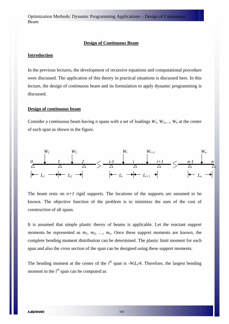
Optimization Methods: Dynamic Programming Applications – Design of Continuous Beam
Design of Continuous Beam
Introduction
In the previous lectures, the development of recursive equations and computational procedure
were discussed. The application of this theory in practical situations is discussed here. In this
lecture, the design of continuous beam and its formulation to apply dynamic programming is
discussed.
Design of continuous beam
Consider a continuous beam having n spans with a set of loadings W1, W2,…, Wn at the center
of each span as shown in the figure.
W1
0
L1
W2
1
L2
2
Wi
i-1
Li
Wi+1
i
Li+1
i+1
Wn
n-1
Ln
n
The beam rests on n+1 rigid supports. The locations of the supports are assumed to be
known. The objective function of the problem is to minimize the sum of the cost of
construction of all spans.
It is assumed that simple plastic theory of beams is applicable. Let the reactant support
moments be represented as m1, m2, …, mn. Once these support moments are known, the
complete bending moment distribution can be determined. The plastic limit moment for each
span and also the cross section of the span can be designed using these support moments.
The bending moment at the center of the ith span is -WiLi/4. Therefore, the largest bending
moment in the ith span can be computed as
A.BENHARIA.BENHARIA.BENHARIA.BENHARI 161

Optimization Methods: Dynamic Programming Applications – Design of Continuous Beam
niforLWmm
mmM iiiiiii ,...2,1
42,,max 1
1 =⎭⎬⎫
⎩⎨⎧
−+
= −−
For a beam of uniform cross section in each span, the limit moment m_limi for the ith span
should be greater than or equal to Mi. The cross section of the beam should be selected in
such a way that it has the required limit moment. Since the cost of the beam depends on the
cross section, which in turn depends on the limit moment, cost of the beam can be expressed
as a function of the limit moments.
If represents the sum of the cost of construction of all spans of the beam where X
represents the vector of limit moments
∑=
n
ii XC
1)(
⎪⎪⎭
⎪⎪⎬
⎫
⎪⎪⎩
⎪⎪⎨
⎧
=
nm
mm
X
lim_
lim_lim_
2
1
M
then, the optimization problem is to find X so that ∑ is minimized while satisfying
the constraints
=
n
ii XC
1)(
niforMm ii ...,,2,1lim_ =≥ .
This problem has a serial structure and can be solved using dynamic programming.
A.BENHARIA.BENHARIA.BENHARIA.BENHARI 162

Optimization Methods: Dynamic Programming Applications – Optimum Geometric Layout of Truss
Optimum Geometric Layout of Truss
Introduction
In this lecture, the optimal design of elastic trusses is discussed from a dynamic programming
point of view. Emphasis is given on minimizing the cost of statically determinate trusses
when the cross-sectional areas of the bars are available.
Optimum geometric layout of truss
Consider a planar, pin jointed cantilever multi bayed truss. Assume the length of the bays to
be unity. The truss is symmetric to the x axis. The geometry or layout of the truss is defined
by the y coordinates (y1, y2, …, yn). The truss is subjected to a unit load W1. The details are
shown in the figure below.
h1
h2
h3
W1=1
y1
y2
y3
y4
x
1 1 1
Consider a particular bay i. Assume the truss is statically determinate. Thus, the forces in the
bars of bay i depend only on the coordinates yi-1 and yi and not on any other coordinates. The
A.BENHARIA.BENHARIA.BENHARIA.BENHARI 163

Optimization Methods: Dynamic Programming Applications – Optimum Geometric Layout of Truss
cross sectional area of a bar can be determined, once the length and force in it are known.
Thus, the cost of the bar can in turn be determined.
The optimization problem is to find the geometry of the truss which will minimize the total
cost from all the bars. For the three bay truss shown above, the relation between y coordinates
can be expressed as
yi+1 = yi + di for i = 1,2,3
This is an initial value problem since the value y1 is already known. Let the y coordinate of
each node is limited to a finite number of values say 0.25, 0.5, 0.75 and 1. Then, as shown in
the figure below, there will be 64 different possible ways to reach y4 from y1.
y1 y4 y3 y2
0.25
0.50
0.75
1.00
This can be represented as a serial multistage initial value decision problem and can be
solved using dynamic programming.
A.BENHARIA.BENHARIA.BENHARI 164

Optimization Methods: Dynamic Programming Applications – Water Allocation
Water Allocation as a Sequential Process – Recursive Equations
Introduction
As discussed in previous lecture notes, in dynamic programming, a problem is handled as a
sequential process or a multistage decision making process. In this lecture, we will explain
how a water allocation problem can be represented as sequential process and can be solved
using backward recursion method of dynamic programming.
Water allocation problem
Consider a canal supplying water to three fields in which three different crops are being
cultivated. The maximum capacity of the canal is given as Q units of water. The three fields
can be denoted as i=1,2,3 and the amount of water allocated to each field as xi.
Field 1
Field 2
Field 3
x1
x3
x2
The net benefits from producing the crops in each field are given by the functions below.
23333
22222
21111
7)(
5.18)(
5.05)(
xxxNB
xxxNB
xxxNB
−=
−=
−=
A.BENHARIA.BENHARIA.BENHARIA.BENHARI 165
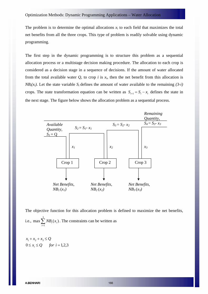
Optimization Methods: Dynamic Programming Applications – Water Allocation
The problem is to determine the optimal allocations xi to each field that maximizes the total
net benefits from all the three crops. This type of problem is readily solvable using dynamic
programming.
The first step in the dynamic programming is to structure this problem as a sequential
allocation process or a multistage decision making procedure. The allocation to each crop is
considered as a decision stage in a sequence of decisions. If the amount of water allocated
from the total available water Q, to crop i is xi, then the net benefit from this allocation is
NBi(xi). Let the state variable Si defines the amount of water available to the remaining (3-i)
crops. The state transformation equation can be written as iii xSS = −+1
3
defines the state in
the next stage. The figure below shows the allocation problem as a sequential process.
Available Quantity, S1 = Q
Crop 1 Crop 2 Crop 3
x1 x2 x3
S2 = S1- x1 S3 = S2- x2
Net Benefits, NB1 (x1)
Net Benefits, NB2 (x2)
Net Benefits, NB3 (x3)
Remaining Quantity, S4 = S3- x3
The objective function for this allocation problem is defined to maximize the net benefits,
i.e., . The constraints can be written as ∑=1
)(maxi
ii xNB
3,2,10321
=≤≤≤++
iforQxQxxx
i
A.BENHARIA.BENHARIA.BENHARI 166
Optimization Methods: Dynamic Programming Applications – Water Allocation
Let be the maximum net benefits that can be obtained from allocating water to crops
1,2 and 3. Thus,
)(1 Qf
⎥⎦
⎤⎢⎣
⎡= ∑
=≥≤++
3
10,,1 )(max)(
321321 i
iixxx
QxxxxNBQf
Transforming this into three problems each having only one decision variable,
⎥⎥
⎦
⎤
⎢⎢
⎣
⎡
⎪⎭
⎪⎬⎫
⎪⎩
⎪⎨⎧
++==−≤≤=−≤≤≤≤
)(max)(max)(max)( 330
220
110
1
32233
2122
11
xNBxNBxNBQfSxSx
xSxQx
xQx
x
Backward recursive equations
Considering the last term of this equation, let be the maximum net benefits from crop
3. The state variable for this stage is which can vary from 0 to Q. Therefore,
)( 33 Sf
3S
)( 22 Sf
)(max)( 330
33
333
xNBSfSx
x≤≤
=
Since , . Thus can be rewritten as 223 xSS −= )()( 22333 xSfSf −= )(1 Qf
{ }⎥⎥⎦
⎤
⎢⎢⎣
⎡−++=
=−≤≤≤≤
)()(max)(max)( 223220
110
1
2122
11
xSfxNBxNBQfSxQx
xQx
x
Now, let be the maximum benefits derived from crops 2 and 3 for a given quantity
which can vary between 0 and Q. Therefore can be written as,
)( 22 Sf 2S
{ })()(max)( 223220
22
2122
xSfxNBSfSxQx
x−+=
=−≤≤
Again, since , which is the maximum total net benefit from the allocation to
the crops 1, 2 and 3, can be rewritten as
12 xQS −= )(1 Qf
A.BENHARIA.BENHARIA.BENHARI 167

Optimization Methods: Dynamic Programming Applications – Water Allocation
[ ])()(max)( 12110
1
11
xQfxNBQfQx
x−+=
≤≤
Now, once the value of is calculated, the value of can be determined, from
which can be determined.
)( 33 Sf )( 22 Sf
)(1 Qf
Forward recursive equations
The procedure explained above can also be solved using a forward proceeding manner. Let
the function be the total net benefit from crops 1 to i for a given input of which is
allocated to those crops. Considering the first stage alone,
)( ii Sf iS
2S )( 22 Sf
)(max)( 1111
111
xNBSfSx
x≤
=
Since, the value of is not known (excepting that should not exceed Q), the equation
above has to be solved for a range of values from 0 to Q. Now, considering the first two crops
together, with units of water available to these crops, can be written as,
1S 1S
[ ])()(max)( 2212222
222
xSfxNBSfSx
x−+=
≤
This equation also should be solved for a range of values for from 0 to Q. Finally,
considering the whole system i.e., crops 1, 2 and 3, can be expressed as,
2S
)( 33 Sf
)( 33 Sf
[ ])()(max)( 3323333
333
xSfxNBSfQSx
x−+=
=≤
Here, if it is given that the whole Q units of water should be allocated, then the value of
can be taken as equal to Q. Otherwise, should be solved for a range of values from 0 to
Q.
3S
A.BENHARIA.BENHARIA.BENHARI 168

Optimization Methods: Dynamic Programming Applications – Water Allocation
The basic equations for the water allocation problem using both the approaches are discussed.
A numerical problem and its solution will be described in the next lecture.
A.BENHARIA.BENHARIA.BENHARI 169
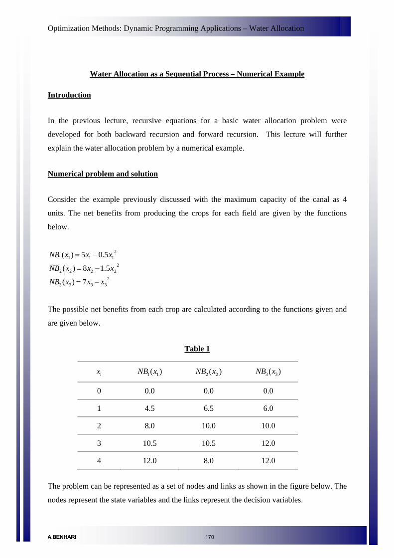
Optimization Methods: Dynamic Programming Applications – Water Allocation
Water Allocation as a Sequential Process – Numerical Example
Introduction
In the previous lecture, recursive equations for a basic water allocation problem were
developed for both backward recursion and forward recursion. This lecture will further
explain the water allocation problem by a numerical example.
Numerical problem and solution
Consider the example previously discussed with the maximum capacity of the canal as 4
units. The net benefits from producing the crops for each field are given by the functions
below.
23333
22222
21111
7)(
5.18)(
5.05)(
xxxNB
xxxNB
xxxNB
−=
−=
−=
The possible net benefits from each crop are calculated according to the functions given and
are given below.
Table 1
ix )( 11 xNB )( 22 xNB )( 33 xNB
0 0.0 0.0 0.0
1 4.5 6.5 6.0
2 8.0 10.0 10.0
3 10.5 10.5 12.0
4 12.0 8.0 12.0
The problem can be represented as a set of nodes and links as shown in the figure below. The
nodes represent the state variables and the links represent the decision variables.
A.BENHARIA.BENHARIA.BENHARIA.BENHARI 170

Optimization Methods: Dynamic Programming Applications – Water Allocation
4
x1 x2 x3
4
3
2
1
0
4
3
2
1
0
0
1
2
3
4
0
1
0
1
2
4
3
2
1
0
0
1
0
1
2
Crop 1 Crop 2 Crop 3
The values inside the nodes show the value of possible state variables at each stage. Number
of nodes for any stage corresponds to the number of discrete states possible for each stage.
The values over the links show the different values taken by decision variables corresponding
to the value taken by state variables. It may be noted that link values for all links are not
shown in the above figure.
Solution using Backward Recursion:
Starting from the last stage, the suboptimization function for the 3rd crop is given as,
)(max)( 330
33
333
xNBSfSx
x≤≤
= with the range of from 0 to 4. 3S
A.BENHARIA.BENHARIA.BENHARI 171
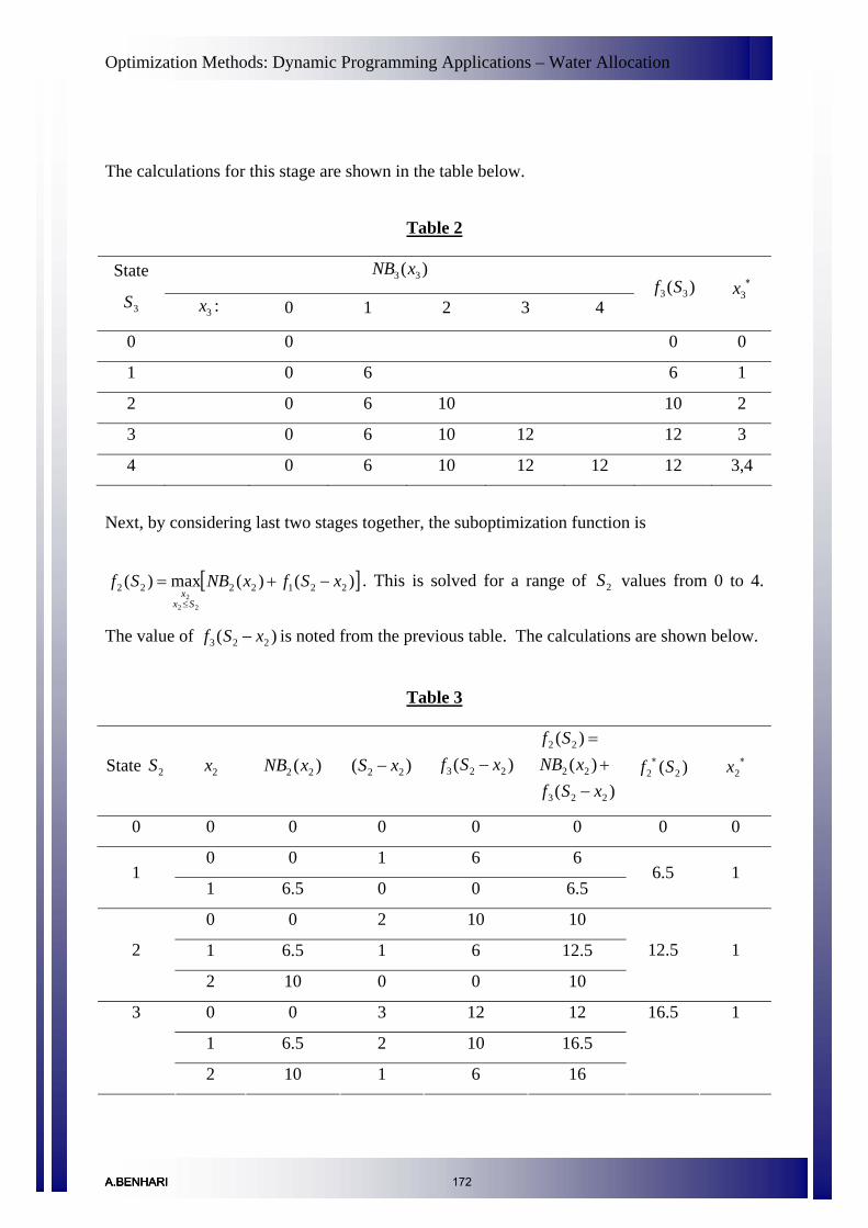
Optimization Methods: Dynamic Programming Applications – Water Allocation
The calculations for this stage are shown in the table below.
Table 2
)( 33 xNB State
3S3x : 0 1 2 3 4
)( 33 Sf ∗3x
0 0 0 0
1 0 6 6 1
2 0 6 10 10 2
3 0 6 10 12 12 3
4 0 6 10 12 12 12 3,4
Next, by considering last two stages together, the suboptimization function is
[ )()(max)( 2212222
222
xSfxNBSfSx
x− ]+=
≤
. This is solved for a range of values from 0 to 4.
The value of is noted from the previous table. The calculations are shown below.
2S
)( 223 xSf −
Table 3
State 2S 2x )( 22 xNB )( 22 xS − )( 223 xSf − )(
)()(
223
22
22
xSfxNB
Sf
−+
= )( 22 Sf ∗ ∗
2x
0 0 0 0 0 0 0 0
0 0 1 6 6 1
1 6.5 0 0 6.5 6.5 1
0 0 2 10 10
1 6.5 1 6 12.5 2
2 10 0 0 10
12.5 1
0 0 3 12 12
1 6.5 2 10 16.5
3
2 10 1 6 16
16.5 1
A.BENHARIA.BENHARIA.BENHARI 172

Optimization Methods: Dynamic Programming Applications – Water Allocation
3 10.5 0 0 10.5
Table contd. on next page
0 0 4 12 12
1 6.5 3 12 18.5
2 10 2 10 20
3 10.5 1 6 16.5
4
4 8 0 0 8
20 2
Finally, by considering all the three stages together, the sub-optimization function is
[ ])()(max)( 12110
1
11
xQfxNBQfQx
x−+=
≤≤
. The value of 41 ==QS . The calculations are shown in
the table below.
Table 4
State
QS =11x )( 11 xNB )( 1xQ − )( 12 xQf −
)()(
)(
12
11
11
xQfxNB
Sf
−+
= )( 11 Sf ∗ ∗
1x
0 0 4 20 20
1 4.5 3 16.5 21
2 8 2 12.5 20.5
3 10.5 1 6.5 17
4
4 12 0 0 12
21 1
Now, backtracking through each table to find the optimal values of decision variables, the
optimal allocation for crop 1, = 1 for a value of 4. This will give the value of
as S . From Table 3, the optimal allocation for crop 2, for is 1. Again,
. Thus, from Table 2 is 2. The maximum total net benefit from all the
crops is 21. The optimal solution is given below
∗x S S
3112 =−= xS 2x 32 =S
S *3x
1 1 2
2223 =−= xS
A.BENHARIA.BENHARIA.BENHARI 173

Optimization Methods: Dynamic Programming Applications – Water Allocation
2
1
1
21
3
2
1
=
=
=
=
∗
∗
∗
∗
x
x
x
f
Solution using Forward Recursion:
While starting to solve from the first stage and proceeding towards the final stage, the
suboptimization function for the first stage is given as,
)(max)( 1111
111
xNBSfSx
x≤
= . The range of values for is from 0 to 4. 1S
Table 5
State 1S 1x )( 11 xNB )( 22 Sf ∗ ∗1x
0 0 0 0 0
0 0 1
1 4.5 4.5 1
0 0
1 4.5 2
2 8
8 2
0 0
1 4.5
2 8 3
3 10.5
10.5 3
0 0
1 4.5
2 8
3 10.5
4
4 12
12 4
A.BENHARIA.BENHARIA.BENHARI 174

Optimization Methods: Dynamic Programming Applications – Water Allocation
Now, considering the first two crops together, can be written as, )( 22 Sf
[ )()(max)( 2212222
222
xSfxNBSfSx
x− ]+=
≤
with ranging from 0 to 4. The calculations for this
stage are shown below.
2S
Table 6
State 2S 2x )( 22 xNB )( 22 xS − )( 221 xSf − )(
)()(
222
22
22
xSfxNB
Sf
−+
= )( 22 Sf ∗ ∗
2x
0 0 0 0 0 0 0 0
0 0 1 4.5 4.5 1
1 6.5 0 0 6.5 6.5 1
0 0 2 8 8
1 6.5 1 4.5 11 2
2 10 0 0 10
11 1
0 0 3 10.5 10.5
1 6.5 2 8 14.5
2 10 1 4.5 14.5 3
3 10.5 0 0 10.5
14.5 1,2
0 0 4 12 12
1 6.5 3 10.5 17
2 10 2 8 18
3 10.5 1 4.5 15
4
4 8 0 0 8
18 2
Now, considering the whole system i.e., crops 1, 2 and 3, can be expressed as, )( 33 Sf
[ ])()(max)( 3323333
333
xSfxNBSfQSx
x−+=
=≤
with the value of 43 =S .
A.BENHARIA.BENHARIA.BENHARI 175

Optimization Methods: Dynamic Programming Applications – Water Allocation
The calculations are shown below.
Table 7
State 3S 3x )( 33 xNB 33 xS − )( 332 xSf − )(
)()(
332
33
33
xSfxNB
Sf
−+
= )( 33 Sf ∗ ∗
3x
0 0 4 18 18
1 6 3 14.5 20.5
2 10 2 11 21
3 12 1 6.5 18.5
4
4 12 0 0 12
21 2
In order to find the optimal solution, a backtracking is done. From Table 7, the optimal value
of is given as 2 for the value of 4. Therefore, *3x 3S 2332 = − =xSS
1=∗x 1
. Now, from Table 6,
the value of . Then, 2 221 =− xS = S and from Table 5, for 11 =S , the value of .
Thus, the optimal values determined are shown below.
1=∗x1
2
1
1
21
3
2
1
=
=
=
=
∗
∗
∗
∗
x
x
x
f
These optimal values are same as those we got by solving using backward recursion method.
A.BENHARIA.BENHARIA.BENHARI 176

Optimization Methods: Dynamic Programming Applications – Capacity Expansion
Capacity Expansion
Introduction
The most common applications of dynamic programming in water resources include water
allocation, capacity expansion of infrastructure and reservoir operation. In this lecture,
dynamic programming formulation for capacity expansion and a numerical example are
discussed.
Capacity expansion
Consider a municipality planning to increase the capacity of its infrastructure (ex: water
treatment plant, water supply system etc) in future. The increments are to be made
sequentially in specified time intervals. Let the capacity at the beginning of time period t be St
(existing capacity) and the required capacity at the end of that time period be Kt. Let be
the added capacity in each time period. The cost of expansion at each time period can be
expressed as a function of and , i.e. C . The problem is to plan the time sequence
of capacity expansions which minimizes the present value of the total future costs subjected
to meet the capacity demand requirements at each time period. Hence, the objective function
of the optimization model can be written as,
tx
tS tx ),( ttt xS
tS
Minimize ∑=
T
tttt xSC
1),(
where is the present value of the cost of adding an additional capacity in the
time period t with an initial capacity . Each period’s final capacity or next period’s initial
capacity should be equal to the sum of initial capacity and the added capacity. Also at the end
of each time period, the required capacity is fixed. Thus, for a time period t, the constraints
can be expressed as
),( ttt xSC tx
TtforKSTtforxSS
tt
ttt
,...,2,1,...,2,1
1
1
=≥=+=
+
+
A.BENHARIA.BENHARIA.BENHARIA.BENHARI 177

Optimization Methods: Dynamic Programming Applications – Capacity Expansion
In some problems, there may be constraints to the amount of capacity added in each time
period i.e. can take only some feasible values. Thus,
tx
tx ttx Ω∈ .
The capacity expansion problem defined above can be solved in a sequential manner using
dynamic programming. The solution procedure using forward recursion and backward
recursion are explained below.
Forward Recursion
Consider the stages of the model to be the time periods in which capacity expansion is to be
made and the state to be the capacity at the end of each time period t, . Let be the
present capacity before expansion and be the minimum present value of total cost of
capacity expansion from present to the time t.
1+tS 1S
)( 1+tt Sf
TK )( 21 Sf
S 1K TK
Stage 1 Stage t
Stage T St
Ct
xt
St+1 S1 S2
C1 CT
x1 xT
ST ST+1
Considering the first stage, the objective function can be written as,
),(min),(min)(
1211
11121
SSSCxSCSf
−==
The values of can be between and where is the required capacity at the end of
time period 1 and is the final capacity required. In other words, should be solved
for a range of values between and . Then considering first two stages, the
suboptimization function is
2S 1K TK 1K
2
A.BENHARIA.BENHARIA.BENHARI 178

Optimization Methods: Dynamic Programming Applications – Capacity Expansion
( )[ ]
( )[ ])(,min
)(,min)(
2312232
2122232
222
222
xSfxxSC
SfxSCSf
xx
xx
−+−=
+=
Ω∈
Ω∈
which should be solved for all values of ranging from to . Hence, in general for a
time period t, the suboptimization function can be represented as
3S 2K TK
( )[ ])(,min)( 1111 tttttttx
xtt xSfxxSCSftt
t
−+−= +−+
Ω∈
+
with constraint as Ttt KSK ≤≤ +1 . For the last stage, i.e. t=T, the function need to
be solved only for
)( 1+TT Sf
TT KS =+1 .
Backward Recursion
The expansion problem can also be solved using a backward recursion approach with some
modifications. Consider the state be the capacity at the beginning of each time period t.
Let be the minimum present value of total cost of capacity expansion in periods t
through T.
tS
)( TT Sf
]
1−tK TK
For the last period T, the final capacity should reach after doing the capacity expansions.
Thus, the objective function can be written as,
TK
( )[ ]TTTx
xTT xSCSfTT
T
,min)(Ω∈
=
This is solved for all values ranging from to . TS 1−TK TK
In general, for a time period t, the function can be expressed as )( tt Sf
( )[ )(,min)( 1 ttttttx
xtt xSfxSCSftt
t
++= +
Ω∈
which should be solved for all discrete values of
ranging from to .
tS
A.BENHARIA.BENHARIA.BENHARI 179
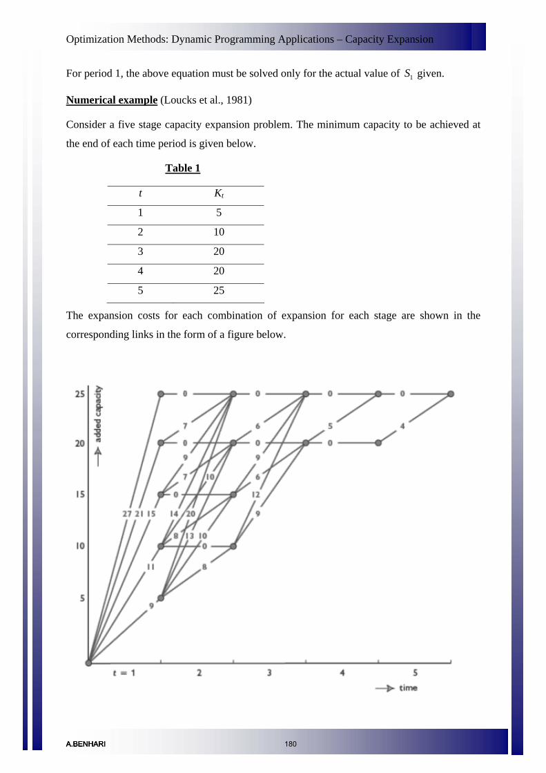
Optimization Methods: Dynamic Programming Applications – Capacity Expansion
For period 1, the above equation must be solved only for the actual value of given. 1S
Numerical example (Loucks et al., 1981)
Consider a five stage capacity expansion problem. The minimum capacity to be achieved at
the end of each time period is given below.
Table 1
t Kt
1 5
2 10
3 20
4 20
5 25
The expansion costs for each combination of expansion for each stage are shown in the
corresponding links in the form of a figure below.
A.BENHARIA.BENHARIA.BENHARI 180

Optimization Methods: Dynamic Programming Applications – Capacity Expansion
Solution Using Forward Recursion
The capacity at the initial stage is given as S1 = 0.
Consider the first stage, t =1. The final capacity for stage 1, S2 can take values between K1 to
K5. Let the state variable can take discrete values of 5, 10, 15, 20 and 25. The objective
function for 1st subproblem with state variable as S2 can be expressed as
),(min),(min)(
1211
11121
SSSCxSCSf
−==
The computations for stage 1 are given in the table below.
Table 2
Stage 1
State Variable, S2Added Capacity,
x1 = S2 – S1C1(S2) f1
*(S2)
5 5 9 9
10 10 11 11
15 15 15 15
20 20 21 21
25 25 27 27
Considering the 1st and 2nd stages together, the state variable S3 can take values from K2 to
K5. Thus, the objective function for 2nd subproblem is
( )[ ]
( )[ ])(,min
)(,min)(
2312232
2122232
222
222
xSfxxSC
SfxSCSf
xx
xx
−++−=
+=
Ω∈
Ω∈
The value of x2 should be taken in such a way that the minimum capacity at the end of stage 2
should be 10, i.e. S . 103 ≥
A.BENHARIA.BENHARIA.BENHARI 181

Optimization Methods: Dynamic Programming Applications – Capacity Expansion
The computations for stage 2 are given in the table below.
Table 3
Stage 2
State
Variable,
S3
Added
Capacity, x2C2(S3)
S2= S3 -
x2f1
*(S2) f2(S3)=C2(S3)+f1*(S2) f2
*(S3)
0 0 10 11 11 10
5 8 5 9 17 11
0 0 15 15 15
5 8 10 11 19 15
10 10 5 9 19
15
0 0 20 21 21
5 7 15 15 22
10 10 10 11 21 20
15 13 5 9 22
21
0 0 25 27 27
5 7 20 21 28
10 9 15 15 24
15 14 10 11 25
25
20 20 5 9 29
24
Like this, repeat this steps till t = 5. For the 5th subproblem, state variable S6 = K5.
A.BENHARIA.BENHARIA.BENHARI 182

Optimization Methods: Dynamic Programming Applications – Capacity Expansion
The computations for stages 3 to 5 are shown in tables below.
Table 4
Stage 3
State
Variable,
S4
Added
Capacity, x3C3(S4)
S3= S4 –
x3f2
*(S3) f3(S4)=C3(S4)+f2*(S3) f3
*(S4)
0 0 20 21 21
5 6 15 15 21 20
10 9 10 11 20
20
0 0 25 24 24
5 6 20 21 27
10 9 15 15 34 25
15 12 10 11 23
23
Table 5
Stage 4
State
Variable,
S5
Added
Capacity, x4C4(S5)
S4= S5 –
x4f3
*(S4) f4(S5)=C4(S5)+f3*(S4) f4
*(S5)
20 0 0 20 20 20 20
0 0 25 23 23 25
5 5 20 20 25 23
A.BENHARIA.BENHARIA.BENHARI 183

Optimization Methods: Dynamic Programming Applications – Capacity Expansion
Table 6
Stage 5
State
Variable,
S6
Added
Capacity, x5C5(S6)
S5= S6 –
x5f4
*(S5) f5(S6)=C5(S6)+f4*(S5) f5
*(S6)
0 0 25 23 23 25
5 4 20 20 24 23
The figure below shows the solutions with the cost of each addition along the links and the
minimum total cost at each node.
From the figure, the optimal cost of expansion is 23 units. By doing backtracking from the
last stage (farthest right node) to the initial stage, the optimal expansion to be done at 1st stage
= 10 units, 3rd stage = 15 units and rest all stages = 0 units.
A.BENHARIA.BENHARIA.BENHARI 184
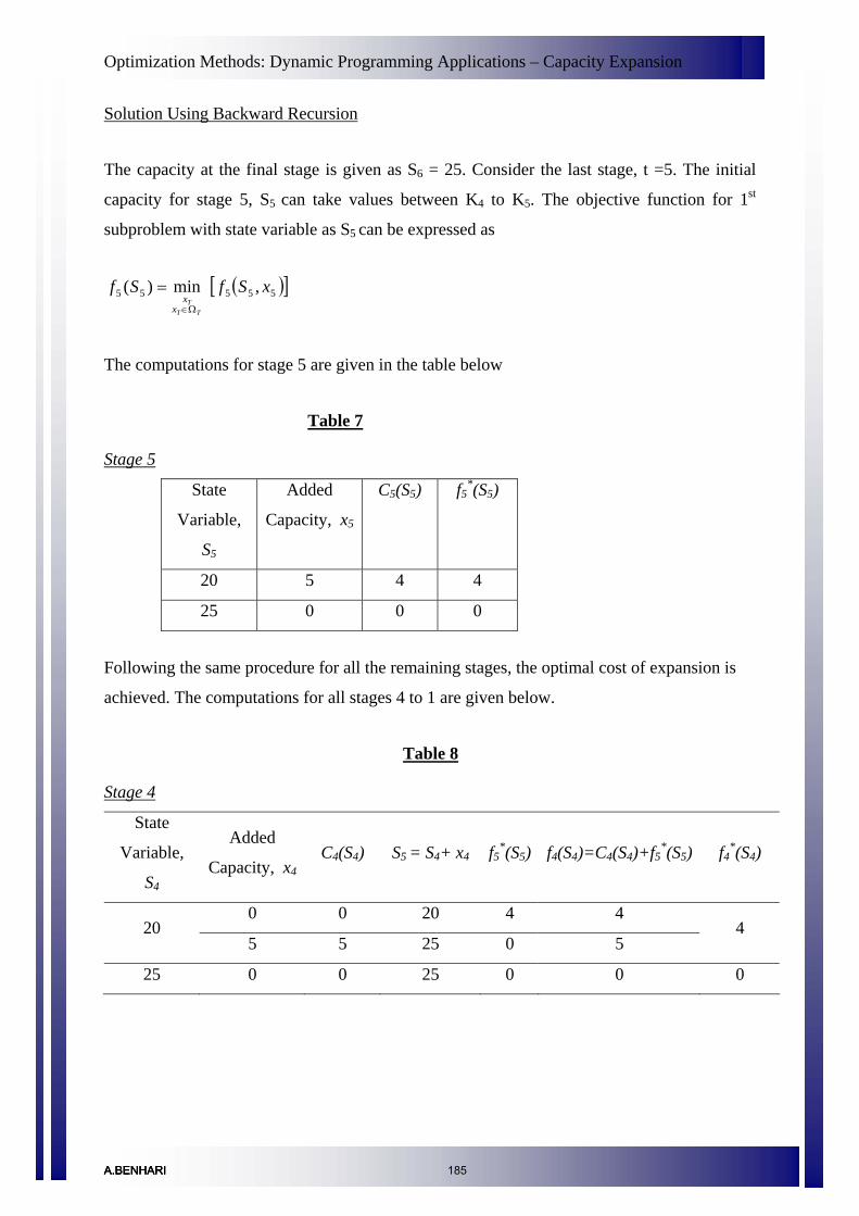
Optimization Methods: Dynamic Programming Applications – Capacity Expansion
Solution Using Backward Recursion
The capacity at the final stage is given as S6 = 25. Consider the last stage, t =5. The initial
capacity for stage 5, S5 can take values between K4 to K5. The objective function for 1st
subproblem with state variable as S5 can be expressed as
( )[ ]55555 ,min)( xSfSfTT
Tx
xΩ∈
=
The computations for stage 5 are given in the table below
Table 7
Stage 5
State
Variable,
S5
Added
Capacity, x5
C5(S5) f5*(S5)
20 5 4 4
25 0 0 0
Following the same procedure for all the remaining stages, the optimal cost of expansion is
achieved. The computations for all stages 4 to 1 are given below.
Table 8
Stage 4
State
Variable,
S4
Added
Capacity, x4C4(S4) S5 = S4+ x4 f5
*(S5) f4(S4)=C4(S4)+f5*(S5) f4
*(S4)
0 0 20 4 4 20
5 5 25 0 5 4
25 0 0 25 0 0 0
A.BENHARIA.BENHARIA.BENHARI 185
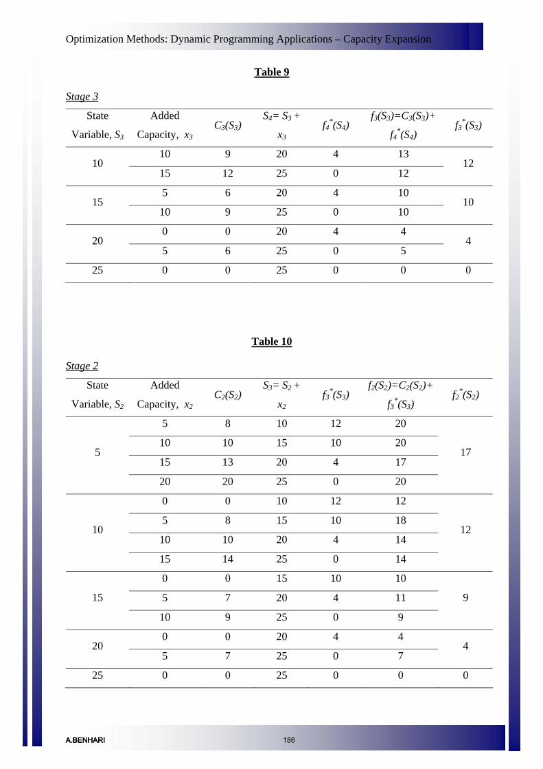
Optimization Methods: Dynamic Programming Applications – Capacity Expansion
Table 9
Stage 3
State
Variable, S3
Added
Capacity, x3C3(S3)
S4= S3 +
x3f4
*(S4) f3(S3)=C3(S3)+
f4*(S4)
f3*(S3)
10 9 20 4 13 10
15 12 25 0 12 12
5 6 20 4 10 15
10 9 25 0 10 10
0 0 20 4 4 20
5 6 25 0 5 4
25 0 0 25 0 0 0
Table 10
Stage 2
State
Variable, S2
Added
Capacity, x2C2(S2)
S3= S2 +
x2f3
*(S3) f2(S2)=C2(S2)+
f3*(S3)
f2*(S2)
5 8 10 12 20
10 10 15 10 20
15 13 20 4 17 5
20 20 25 0 20
17
0 0 10 12 12
5 8 15 10 18
10 10 20 4 14 10
15 14 25 0 14
12
0 0 15 10 10
5 7 20 4 11 15
10 9 25 0 9
9
0 0 20 4 4 20
5 7 25 0 7 4
25 0 0 25 0 0 0
A.BENHARIA.BENHARIA.BENHARI 186
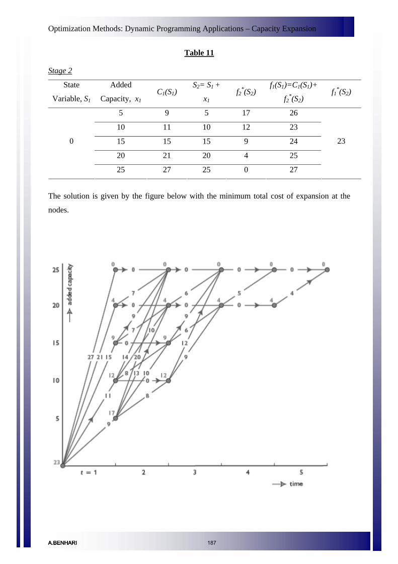
Optimization Methods: Dynamic Programming Applications – Capacity Expansion
Table 11
Stage 2
State
Variable, S1
Added
Capacity, x1C1(S1)
S2= S1 +
x1f2
*(S2) f1(S1)=C1(S1)+
f2*(S2)
f1*(S2)
5 9 5 17 26
10 11 10 12 23
15 15 15 9 24
20 21 20 4 25
0
25 27 25 0 27
23
The solution is given by the figure below with the minimum total cost of expansion at the
nodes.
A.BENHARIA.BENHARIA.BENHARI 187

Optimization Methods: Dynamic Programming Applications – Capacity Expansion
The optimal cost of expansion is obtained from the node value at the first node i.e. 23 units
which is the same as obtained from forward recursion. The optimal expansions at each time
period can be obtained by moving forward from the first node to the last node. Thus, the
optimal expansions to be made are 10 units at the first stage and 15 units at the last stage.
Hence the final requirement of 25 units is achieved.
Although this type of expansion problem can be solved, the future demand and the future cost
of expansion are highly uncertain. Hence, the solution obtained cannot be used for making
expansions till the end period, T. It can be very well used to make decisions about the
expansion to be done in the current period. For this to be done, the final period T should be
selected far away from the current period, so that the uncertainty on current period decisions
is much less.
It may be note that, generally water supply projects are planned for a period of 25-30 years to
avoid undue burden to the present generation. In addition, change of value of money in time
(due to inflation and other aspects) is not considered in the examples above.
A.BENHARIA.BENHARIA.BENHARI 188

Optimization Methods: Dynamic Programming Applications – Reservoir Operation
Reservoir Operation
Introduction
In the previous lectures, we discussed about the application of dynamic programming in
water allocation and capacity expansion of infrastructure. Another major application is in the
field of reservoir operation, which will be discussed in this lecture.
Reservoir operation – Steady state optimal policy
Consider a single reservoir receiving inflow and making releases for each time period t.
The maximum capacity of the reservoir is K. The optimization problem is to find the
sequence of releases to be made from the reservoir that maximizes the total net benefits.
These benefits may be from hydropower generation, irrigation, recreation etc. Let and
be the initial and final storages for time period t. Expressing net benefits as a function of ,
and , the net benefit for period t is
ti tr
tS 1+tS
1+tS tr
tS
( )tttt rSSNB ,, 1+ .
If there are T periods in a year, then the objective function is to maximize the total net
benefits from all periods.
Maximize ( )∑=
+
T
ttttt rSSNB
11,,
This is subject to continuity and also capacity constraints. Neglecting all minor losses like
evaporation, seepage etc and assuming that there is no overflow, the continuity relation can
be written as,
TtforriSS tttt ,...2,11 =−+=+
The capacity constraint can be expressed as,
TtforKSt ,...2,1=≤
A.BENHARIA.BENHARIA.BENHARIA.BENHARI 189

Optimization Methods: Dynamic Programming Applications – Reservoir Operation
The above formulated problem can be solved as a sequential process either using forward or
backward approach. Here the stages are the time periods and the states are the storage
volumes.
Assume that there are T periods in a year. In order to find the steady state policy, select a
period in a particular year in the near future (to get steady solution). Usually in almost all
problems, the last period T is taken as the terminal period. At this stage, the optimal release
will be independent of the inflow and also the net benefit .
tr
ti tNB
Now, consider the terminal period as T of a particular year after which reservoir is no longer
useful. Solving this problem in a backward recursion method, let t represents the period in a
year from T to 1 and n represents the periods remaining from t till end. Thus, t will take
values starting from T, decreasing to 1 (which will complete one year) and then again taking
a value of T and repeating the values. The value of n starts from 1 (while considering the Tth
period of last year) and while moving backwards its value keeps on increasing i.e. at the
beginning of the last year, the value of n = T and at the beginning of second last year its
value will be equal to 2T and so on.
Starting from T of last year, which is at the far right, there is only one period remaining.
Thus, in this case t=T and n=1. Let ( )TT Sf 1
( )TT Sf 1
be the maximum net benefit in the last period of
the year considered. can be expressed as
( ) ( ){ }[ ]TTTTTT
KiSriSr
rTT rriSSNBSf
TTTTTT
T
,,max0
1 −+=
−+≥+≤
≥
which should be solved for all S values from 0 to K. T
Considering the last two stages together for which t=T-1 and n=2, the objective function can
be written as
A.BENHARIA.BENHARIA.BENHARI 190
Optimization Methods: Dynamic Programming Applications – Reservoir Operation
( ) ( ){ } ( )[ ]1111
111111012
1 ,,max
111111
1−−−−−−−−−
−+≥+≤
≥−− −++−+=
−−−−−−
−TTTTTTTTTT
KiSriSr
rTT riSfrriSSNBSf
TTTTTT
T
This also is solved for all values from 0 to K. 1−TS
In general, for a period t of a particular year with n periods remaining, the function can be
written as
( ) ( ){ } ( )[ ]tttn
ttttttt
KiSriSr
rtn
t riSfrriSSNBSf
tttttt
t
−++−+= −+
−+≥+≤≥
110
,,max
where the index t decreases from T to 1 and then takes the value T again for the previous year
and the cycle repeats while the index n starts from 1 and increases at each successive stage.
This cycle can be repeated till the optimum values of for an initial storage will be the
same as the corresponding and of previous year. Such a solution is called stationary
solution. The maximum net benefit can be obtained as the difference of and
tr tS
tr tS
( )tTn
t Sf + ( )tn
t Sf
tS
for any and t.
Numerical example (Loucks et al., 1981)
Consider a reservoir for which the desirable constant storage is 20 units and the constant
release is 25 units. The capacity of the reservoir is 30 units and the inflows for three seasons
are given as 10, 50 and 20 units. The problem is to find the optimum and that
minimizes the total squared deviation from the release and storage targets given. Hence, the
objective function is
tS tr
( ) ( )[ ]22 2520 rS −+− S
tr
tt . Let take the discrete values of 0, 10, 20, 30
and take the values of 10, 20, 30, 40.
t
Solution:
A.BENHARIA.BENHARIA.BENHARI 191

Optimization Methods: Dynamic Programming Applications – Reservoir Operation
Consider a year after which the reservoir is no longer useful. The problem can be expressed
as a sequential process as shown in the figure below
Here no. of seasons (periods), T = 3. Considering the last period for which t = 3 and n = 1,
the optimization function is
Minimize ( ) ( ) ( )[ ]23
233
13 2520 rSSf −+−=
Inflow for 3rd season, I3 = 20 units and capacity of the reservoir, K = 30 units.
The release constraints can be expressed as
203
333
+≤+≤
SISr
and
30203
333
−+≥−+≥
SKISr
The computation for the first subproblem (n = 1) is shown in the table below.
A.BENHARIA.BENHARIA.BENHARI 192

Optimization Methods: Dynamic Programming Applications – Reservoir Operation
Table 1
State variable,
S3Release, r3 ( ) ( )3
23 2520 rS −+− ( )3
13 Sf
Optimal
release, r3*
10 625 0
20 425 425 20
10 325
20 125 10
30 125
125 20, 30
10 225
20 25
30 25 20
40 225
25 20, 30
10 325
20 125
30 125 30
40 325
125 20, 30
Now considering the last two periods (n =2), the optimization function is
Minimize ( ) ( ) ( )[ ] ( )2221
32
22
222
2 2520 rISfrSSf −++−+−=
Inflow for 2nd season, I2 = 50 units. The release constraints can be expressed as
5022 +≤ Sr and
305022 −+≥ Sr
The computation for the second subproblem (n = 2) is shown in the table below.
For S2=30, i.e. . Since r50..3050 222 ≥−+≥ reiSr 502 ≥r 2 can take values only of 10,
20, 30 and 40 only, the release cannot be made for S2=30.
Table 2
A.BENHARIA.BENHARIA.BENHARI 193
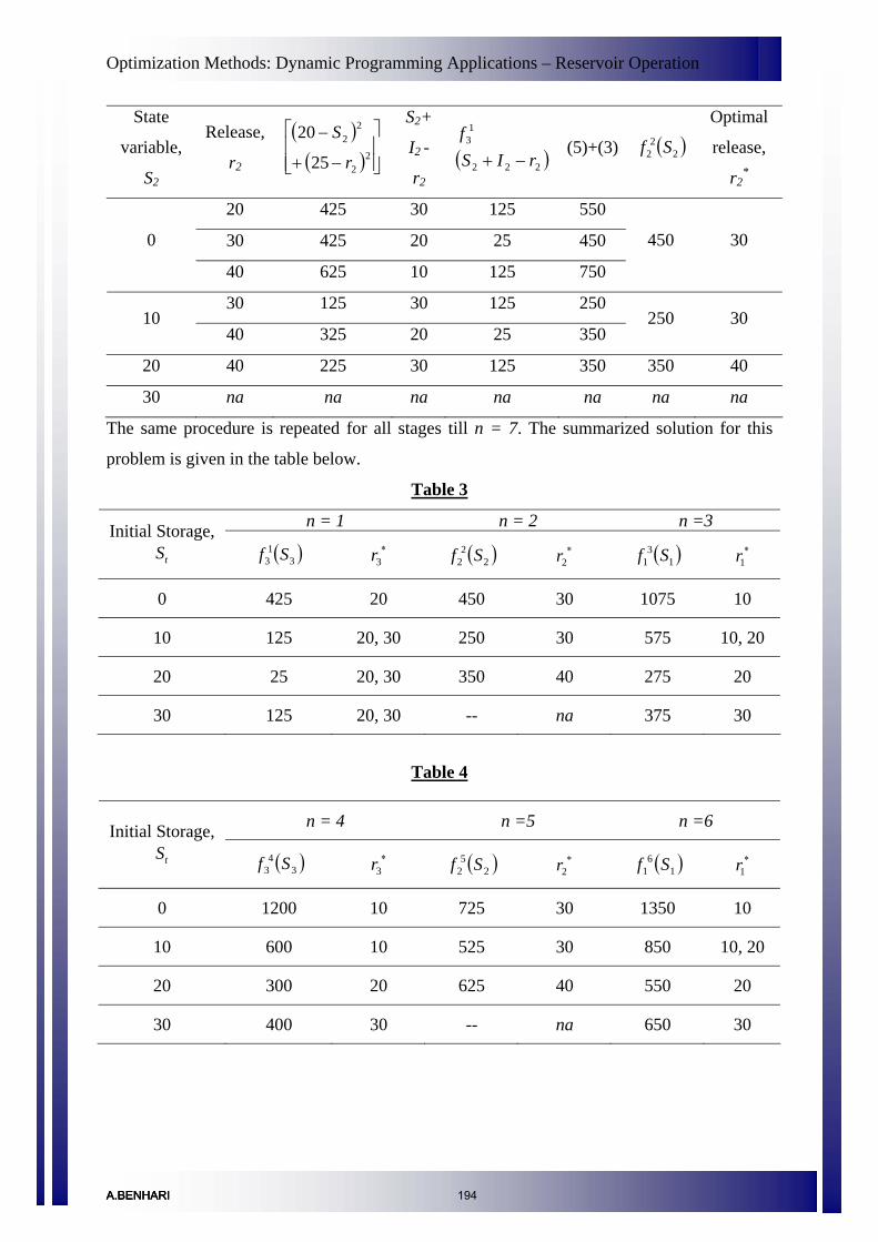
Optimization Methods: Dynamic Programming Applications – Reservoir Operation
State
variable,
S2
Release,
r2
( )( ) ⎥
⎥⎦
⎤
⎢⎢⎣
⎡
−+
−2
2
22
25
20
r
SS2+
I2 -
r2
( )222
13
rISf
−+(5)+(3) ( )2
22 Sf
Optimal
release,
r2*
20 425 30 125 550
30 425 20 25 450 0
40 625 10 125 750
450 30
30 125 30 125 250 10
40 325 20 25 350 250 30
20 40 225 30 125 350 350 40
30 na na na na na na na
The same procedure is repeated for all stages till n = 7. The summarized solution for this
problem is given in the table below.
Table 3
n = 1 n = 2 n =3 Initial Storage, tS ( )3
13 Sf ∗
3r ( )22
2 Sf ∗2r ( )1
31 Sf ∗
1r
0 425 20 450 30 1075 10
10 125 20, 30 250 30 575 10, 20
20 25 20, 30 350 40 275 20
30 125 20, 30 -- na 375 30
Table 4
n = 4 n =5 n =6 Initial Storage, tS ( )3
43 Sf ∗
3r ( )25
2 Sf ∗2r ( )1
61 Sf ∗
1r
0 1200 10 725 30 1350 10
10 600 10 525 30 850 10, 20
20 300 20 625 40 550 20
30 400 30 -- na 650 30
A.BENHARIA.BENHARIA.BENHARI 194
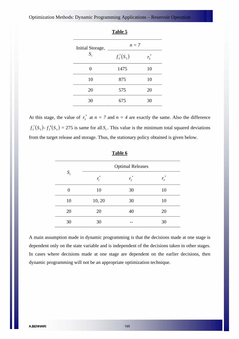
Optimization Methods: Dynamic Programming Applications – Reservoir Operation
Table 5
n = 7 Initial Storage, tS ( )3
73 Sf ∗
3r
0 1475 10
10 875 10
20 575 20
30 675 30
At this stage, the value of at n = 7 and n = 4 are exactly the same. Also the difference
- = 275 is same for all . This value is the minimum total squared deviations
from the target release and storage. Thus, the stationary policy obtained is given below.
∗3r
( )37
3 Sf ( )34
3 Sf tS
Table 6
Optimal Releases tS
∗1r ∗
2r ∗3r
0 10 30 10
10 10, 20 30 10
20 20 40 20
30 30 -- 30
A main assumption made in dynamic programming is that the decisions made at one stage is
dependent only on the state variable and is independent of the decisions taken in other stages.
In cases where decisions made at one stage are dependent on the earlier decisions, then
dynamic programming will not be an appropriate optimization technique.
A.BENHARIA.BENHARIA.BENHARI 195

Optimization Methods: Dynamic Programming Applications – Reservoir Operation
M6L6A.BENHARIA.BENHARIA.BENHARI 196

Optimization Methods: Integer Programming – Integer Linear Programming
Integer Linear Programming
Introduction
In all the previous lectures in linear programming discussed so far, the design variables
considered are supposed to take any real value. However in practical problems like
minimization of labor needed in a project, it makes little sense in assigning a value like 5.6 to
the number of labourers. In situations like this, one natural idea for obtaining an integer
solution is to ignore the integer constraints and use any of the techniques previously
discussed and then round-off the solution to the nearest integer value. However, there are
several fundamental problems in using this approach:
1. The rounded-off solutions may not be feasible.
2. The objective function value given by the rounded-off solutions (even if some are
feasible) may not be the optimal one.
3. Even if some of the rounded-off solutions are optimal, checking all the rounded-off
solutions is computationally expensive ( possible round-off values to be considered
for an variable problem)
n2
n
Types of Integer Programming
When all the variables in an optimization problem are restricted to take only integer values, it
is called an all – integer programming problem. When the variables are restricted to take only
discrete values, the problem is called a discrete programming problem. When only some
variable values are restricted to take integer or discrete, it is called mixed integer or discrete
programming problem. When the variables are constrained to take values of either zero or 1,
then the problem is called zero – one programming problem.
Integer Linear Programming
Integer Linear Programming (ILP) is an extension of linear programming, with an additional
restriction that the variables should be integer valued. The standard form of an ILP is of the
form,
A.BENHARIA.BENHARIA.BENHARIA.BENHARI 197

Optimization Methods: Integer Programming – Integer Linear Programming
0
max
≥≤
XbAXtosubject
XcT
X must be integer valued
The associated linear program dropping the integer restrictions is called linear relaxation LR.
Thus, LR is less constrained than ILP. If the objective function coefficients are integer, then
for minimization, the optimal objective for ILP is greater than or equal to the rounded-off
value of the optimal objective for LR. For maximization, the optimal objective for ILP is less
than or equal to the rounded-off value of the optimal objective for LR.
For a minimization ILP, the optimal objective value for LR is less than or equal to the
optimal objective for ILP and for a maximization ILP, the optimal objective value for LR is
greater than or equal to that of ILP. If LR is infeasible, then ILP is also infeasible. Also, if LR
is optimized by integer variables, then that solution is feasible and optimal for IP.
A most popular method used for solving all-integer and mixed-integer linear programming
problems is the cutting plane method by Gomory (Gomory, 1957).
Gomory’s Cutting Plane Method for All – Integer Programming
Consider the following optimization problem.
0,4593
62tosubject3Maximize
21
21
21
21
≥≤+≤−+=
xxxx
xxxxZ
x1 and x2 are integers
The graphical solution for the linear relaxation of this problem is shown below.
A.BENHARIA.BENHARIA.BENHARI 198

Optimization Methods: Integer Programming – Integer Linear Programming
0 1 2 3 4 5 6 70
1
2
3
4
5
6
7
D C
B
A
x1
x2
It can be seen that the solution is 733,7
54 21 == xx and the optimal value of 7417=Z .
The feasible solutions accounting the integer constraints are shown by red dots. These points
are called integer lattice points. The original feasible region is reduced to a new feasible
region by including some additional constraints such that an extreme point of the new
feasible region becomes an optimal solution after accounting for the integer constraints.
The graphical solution for the example previously discussed taking x1 and x2 as integers are
shown below. Two additional constraints (MN and OP) are included so that the original
feasible region ABCD is reduced to a new feasible region AEFGCD. Thus the solution for
this ILP is and the optimal value is3,4 21 == xx 15=Z .
7417=Z
( )733,7
54
62 21
− xx
4593 21
≤
+ ≤xx
A.BENHARIA.BENHARIA.BENHARI 199

Optimization Methods: Integer Programming – Integer Linear Programming
0 1 2 3 4 5 6 70
1
2
3
4
5
6
7
D C
B
A
Additional constraints
G
E
F
x1
x2
(4,3)
O
P
M
N
( )733,7
54 7
417=Z
15=Z
Gomary proposed a systematic method to develop these additional constraints known as
Gomory constraints.
Generation of Gomory Constraints:
Let the final tableau of an LP problem consist of n basic variables (original variables) and m
non basic variables (slack variables) as shown in the table below. The basic variables are
represented as xi (i=1,2,…,n) and the non basic variables are represented as yj (j=1,2,…,m).
A.BENHARIA.BENHARIA.BENHARI 200

Optimization Methods: Integer Programming – Integer Linear Programming
Table 1
Variables Basis Z
1x 2x … ix … nx 1y 2y … jy … my rb
Z 1 0 0 0 0 c1 c2 cj cm b
1x 0 1 0 0 0 c11 c12 c1j c1m 1b
2x 0 0 1 0 0 c21 c22 c2j c2m 2b
…
ix 0 0 0 1 0 c31 c32 c3j c3m ib
…
nx 0 0 0 0 1 c41 c42 c4j c4m nb
Choose any basic variable with the highest fractional value. If there is a tie between two
basic variables, arbitrarily choose any of them as . Then from the i
ix
ix th equation of table,
∑=
−=m
jjijii ycbx
1 ……..(1)
Express both and as an integer value plus a fractional part. ib ijc
)3........()2........(
ijijij
iii
ccbb
αβ+=+=
where ib , ijc denote the integer part and iβ , ijα denote the fractional part. iβ will be a
strictly positive fraction ( 10 << i )β and ijα is a non-negative fraction ( )10 <≤ ijα .
Substituting equations (2) and (3) in (1), equation (1) can be written as
∑∑==
−−=−m
jjijiij
m
jiji ycbxy
11αβ …….(4)
For all the variables and to be integers, the right hand side of equation (4) should be
an integer.
ix jy
=−∑=
j
m
jiji y
1αβ integer ……(5)
A.BENHARIA.BENHARIA.BENHARI 201
Optimization Methods: Integer Programming – Integer Linear Programming
Since ijα are non-negative integers and are non-negative integers, the term will
always be a non-negative number. Thus we have,
jy j
m
jij y∑
=1α
11
<≤⎟⎟
⎠
⎞
⎜⎜
⎝
⎛−∑
=ij
m
jiji y βαβ …….(6)
Hence the constraint can be expressed as
01
≤−∑=
j
m
jiji yαβ …….(7)
By introducing a slack variable (which should also be an integer), the Gomory constraint
can be written as
is
ij
m
jiji ys βα −=−∑
=1 …….(8)
General procedure for solving ILP:
1. Solve the given problem as an ordinary LP problem neglecting the integer
constraints. If the optimum values of the variables are integers itself, then there is
nothing more to be done.
2. If any of the basic variables has fractional values, introduce the Gomory constraints
as discussed in the previous section. Insert a new row with the coefficients of this
constraint, to the final tableau of the ordinary LP problem (Table 1).
3. Solve this by applying the dual simplex method.
Since the value of 0=jy in Table 1, the Gomory constraint equation becomes
iis β−= which is a negative value and thus infeasible. Dual simplex method
is used to obtain a new optimal solution that satisfies the Gomory constraint.
4. Check whether the new solution is all-integer or not. If all values are not integers,
then a new Gomory constraint is developed from the new simplex tableau and the
dual simplex method is applied again.
5. This process is continued until an optimal integer solution is obtained or it shows that
the problem has no feasible integer solution.
A.BENHARIA.BENHARIA.BENHARI 202

Optimization Methods: Integer Programming – Integer Linear Programming
Thus, the fundamental idea behind cutting planes is to add constraints to a linear program
until the optimal basic feasible solution takes on integer values. Gomory cuts have the
property that they can be generated for any integer program, but has the disadvantage that the
number of constraints generated can be enormous depending upon the number of variables.
A.BENHARIA.BENHARIA.BENHARI 203
Optimization Methods: Integer Programming – Mixed Integer Programming
Mixed Integer Programming
Introduction
In the previous lecture we have discussed the procedure for solving integer linear
programming in which all the decision variables are restricted to take only integer values. In a
Mixed Integer Programming (MIP) model, some of the variables are real valued and some are
integer valued. When the objective function and constraints for a MIP are all linear, then it is
a Mixed Integer Linear Program (MILP). Although Mixed Integer Nonlinear Programs
(MINLP) also exists, in this chapter we will be dealing with MILP only.
Mixed Integer Programming
In mixed integer programming (MIP), only some of the decision and slack variables are
restricted to take integer values. Gomory cutting plane method is used popularly to solve MIP
and the solution procedure is similar in many aspects to that of all-integer programming. The
first step is to solve the MIP problem as an ordinary LP problem neglecting the integer
restrictions. The procedure ends if the values of the basic variables which are constrained to
take only integer values happen to be integers in this optimal solution. If not, a Gomory
constraint is developed for the basic variable with integer restriction and has largest fractional
value which is explained below. The rest of the procedure is same as that of all-integer
programming.
Generation of Gomory Constraints:
Let be the basic variable which has integer restriction and also has largest fractional value
in the optimal solution of ordinary LP problem. Then from the i
ixth equation of table,
∑=
−=m
jjijii ycbx
1
As explained in all-integer programming, express as an integer value plus a fractional part. ib
iii bb β+=
ijc can be expressed as
A.BENHARIA.BENHARIA.BENHARIA.BENHARI 204

Optimization Methods: Integer Programming – Mixed Integer Programming
−+ += ijijij ccc
where
⎪⎩
⎪⎨⎧
<
≥=
⎪⎩
⎪⎨⎧
<
≥=
−
+
0
00
00
0
ijij
ijij
ij
ijijij
cifc
cifc
cif
cifcc
Therefore,
( ) ( )iiij
m
jijij xbycc −+=+∑
=
−+ β1
Since is restricted to be an integer, ix ib is also an integer and 10 << iβ , the value of
( )iii xb −+β can be or <0. 0≥
Case I: ( )iii xb −+β 0≥
For to be an integer, ix ( ) ,....21 ++=−+ iiiiii ororxb ββββ
Therefore,
( ) ij
m
jijij ycc β≥+∑
=
−+
1
Finally it takes the form
ij
m
jij yc β≥∑
=
+
1
Case II: ( )iii xb −+β <0
For to be an integer, ix
( ) ,....321 iiiiii ororxb ββββ +−+−+−=−+
Therefore,
( ) 11
−≤+∑=
−+ij
m
jijij ycc β
A.BENHARIA.BENHARIA.BENHARI 205

Optimization Methods: Integer Programming – Mixed Integer Programming
Finally it takes the form
11
−≤∑=
−ij
m
jij yc β
Dividing this inequality by ( 1−i )β and multiplying with iβ , we have
ij
m
jij
i
i yc βββ
≥− ∑
=
−
11
Considering both cases I and II, the final form of the inequality becomes (since one of the
inequalities should be satisfied)
ij
m
jij
i
ij
m
jij ycyc β
ββ
≥−
+ ∑∑=
−
=
+
11 1
Then, the Gomory constraint after introducing a slack variable is is
ij
m
jij
i
ij
m
jiji ycycs β
ββ
−=−
−− ∑∑=
−
=
+
11 1
Generate the Gomory constraint for the variables having integer restrictions. Insert this
constraint as the last row of the final tableau of LP problem and solve this using dual simplex
method. MIP techniques are useful for solving pure-binary problems and any combination of
real, integer and binary problems.
A.BENHARIA.BENHARIA.BENHARI 206

Optimization Methods: Integer Programming - Examples
Integer Programming - Examples
Introduction
In the previous two lectures, we have discussed about the procedures for solving integer
linear programming and also mixed integer linear programming. In this lecture we will be
discussing a few examples based on the methods already discussed.
Example of Cutting plane method for ILP:
These steps are explained using the example previously discussed.
0,4593
62tosubject3Maximize
21
21
21
21
≥≤+≤−+=
xxxx
xxxxZ
x1 and x2 are integers
The standard form for the problem can be written as
0,,,4593
62tosubject3Maximize
2121
221
121
21
≥=++
=+−+=
yyxxyxx
yxxxxZ
areyandyxx 2121 ,, integers
Step 1: Solve the problem as an ordinary LP problem neglecting the integer requirements.
Table 1
Variables Iteration Basis
Z
1x 2x 1y 2y rb
rs
r
cb
Z 1 -3 -1 0 0 0 --
1y 0 2 -1 1 0 6 3
1
2y 0 3 9 0 1 45 15
A.BENHARIA.BENHARIA.BENHARIA.BENHARI 207

Optimization Methods: Integer Programming - Examples
Table 2
Variables Iteration Basis Z
1x 2x 1y 2y rb
rs
r
cb
Z 1 0 25
− 23 0 9 --
1x 0 1 21
− 21 0 3 -- 2
2y 0 0 221
23
− 1 36 724
Table 3
Variables Iteration Basis Z
1x 2x 1y 2y rb
rs
r
cb
Z 1 0 0 78
215
7123 --
1x 0 1 0 146
211
733 -- 3
2x 0 0 1 71
− 212
724 --
Optimum value of Z is 7
123 as shown above. Corresponding values of basic variables
are 754
733
1 ==x , 733
724
2 ==x and those of non-basic variables are all zero
(i.e., ). The values are not integers. 021 == yy
Step 2: Introduce Gomory constraints.
Gomory constraint is developed for which is having high fractional value. From the row
corresponding to in the last table, we can write,
1x
1x
211 211
146
733 yyx −−=
A.BENHARIA.BENHARIA.BENHARI 208

Optimization Methods: Integer Programming - Examples
Here 2110,21
1,146,0,14
6,75,4,7
331212121111111 ========= ααβ andccccbb ii .
From Eqn. Gomory constraint can be expressed as
211
211
146.,. 211
12121111
−=−−
−=−−
yysei
yys βαα
By inserting a new row with the coefficients of this constraint to the last table, we get
Table 4
Variables rb Iteration Basis Z
1x 2x 1y 2y 1s
Z 1 0 0 78
215 0
7123
1x 0 1 0 146
211 0
733
2x 0 0 1 71
− 212 0
724
1s 0 0 0 146
− 211
− 1 75
−
Step 3: Solve using dual simplex method
Table 5
Variables rb Iteration Basis Z
1x 2x 1y 2y 1s
Z 1 0 0 78
215 0
7123
1x 0 1 0 146
211 0
733
2x 0 0 1 71
− 212 0
724
1s 0 0 0 146
− 211
− 1 75
−
Ratio -- -- 38 5 --
A.BENHARIA.BENHARIA.BENHARI 209
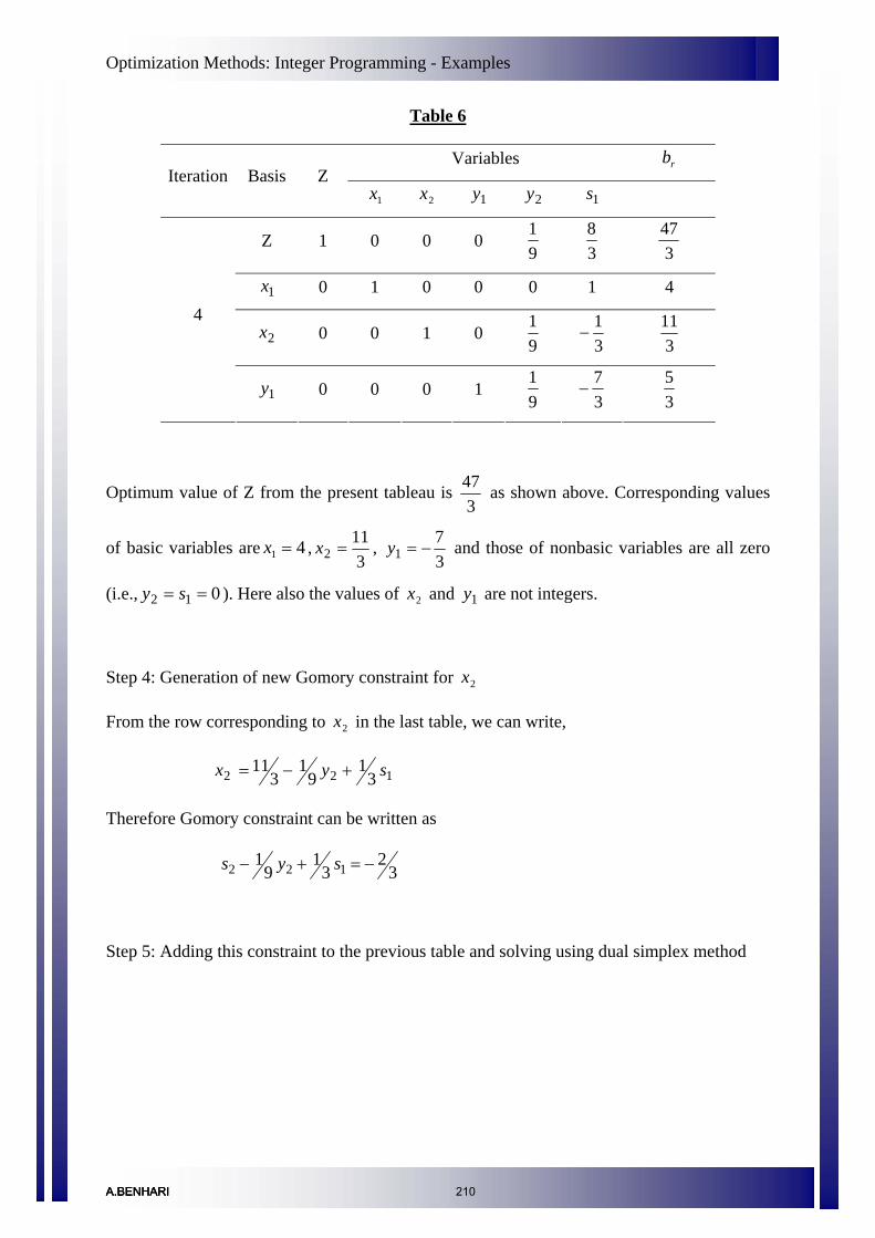
Optimization Methods: Integer Programming - Examples
Table 6
Variables rb Iteration Basis Z
1x 2x 1y 2y 1s
Z 1 0 0 0 91
38
347
1x 0 1 0 0 0 1 4
2x 0 0 1 0 91
31
− 3
11 4
1y 0 0 0 1 91
37
− 35
Optimum value of Z from the present tableau is 3
47 as shown above. Corresponding values
of basic variables are ,41 =x3
112 =x ,
37
1 −=y and those of nonbasic variables are all zero
(i.e., ). Here also the values of and are not integers. 012 == sy 2x 1y
Step 4: Generation of new Gomory constraint for 2x
From the row corresponding to in the last table, we can write, 2x
122 31
91
311 syx +−=
Therefore Gomory constraint can be written as
32
31
91
122 −=+− sys
Step 5: Adding this constraint to the previous table and solving using dual simplex method
A.BENHARIA.BENHARIA.BENHARI 210

Optimization Methods: Integer Programming - Examples
Table 7
Variables rb Iteration Basis Z
1x 2x 1y 2y 1s 2s
Z 1 0 0 0 91
38 0
347
1x 0 1 0 0 0 1 0 4
2x 0 0 1 0 91
31
− 0 3
11
1y 0 0 0 1 91
37
− 0 35
2s 0 0 0 0 91
− 0 31
32
−
Ratio -- -- -- 1 -- -- --
Table 8
Variables rb Iteration Basis Z
1x 2x 1y 2y 1s 2s
Z 1 0 0 0 0 38
31 15
1x 0 1 0 0 0 1 0 4
2x 0 0 1 0 0 31
− 31 3
1y 0 0 0 1 0 37
− 31 1
5
2s 0 0 0 0 1 0 -3 6
The solution from this tableau is 0,6,1,3,4 122121 ====== sysyxx and the value of Z =
15. These are satisfying the integer requirement and hence the desired solution.
A.BENHARIA.BENHARIA.BENHARI 211

Optimization Methods: Integer Programming - Examples
Example of Cutting plane method for MILP
Consider the example previously discussed with integer constraint only on . 2x
The standard form for the problem is
0,,,4593
62tosubject3Maximize
2121
221
121
21
≥=++
=+−+=
yyxxyxx
yxxxxZ
2x should be an integer
Step 1: Solve the problem as an ordinary LP problem. The final tableau is showing the
optimal solutions are shown below.
Table 9
Variables Iteration Basis Z
1x 2x 1y 2y rb
rs
r
cb
Z 1 0 0 78
215
7123 --
1x 0 1 0 146
211
733 -- 3
2x 0 0 1 71
− 212
724 --
Optimum value of Z is 7
123 and corresponding values of basic variables are 754
733
1 ==x ,
733
724
2 ==x and those of non-basic variables are all zero (i.e., 021 == yy ). This is not
satisfying the constraint of to be an integer. 2x
Step 2: Generate Gomory constraint.
Gomory constraint is developed for .From the row corresponding to in the last table,
we can write,
2x 2x
122 212
71
724 yyx −+=
A.BENHARIA.BENHARIA.BENHARI 212

Optimization Methods: Integer Programming - Examples
Here 212,7
1,724
22212 −=== ccb .
Since 222 β+= bb as per Eqn(), the value of 32 =b and 73
2 =β .
Similarly −+ += 212121 ccc and −+ += 222222 ccc .
Therefore,
71,0 2121 −== −+ cc since 21c is negative
0,212
2222 == −+ cc since 22c is positive
Thus Gomory constraint can be written as
ij
m
jij
i
ij
m
jiji ycycs β
ββ
−=−
−− ∑∑=
−
=
+
11 1
73
283
212.,. 122 −=−− yysei
Insert this constraint as the last row of the final tableau.
Table 10
Variables rb Iteration Basis Z
1x 2x 1y 2y 2s
Z 1 0 0 78
215 0
7123
1x 0 1 0 146
211 0
733
2x 0 0 1 71
− 212 0
724
2s 0 0 0 283
−212
− 1 73
−
A.BENHARIA.BENHARIA.BENHARI 213

Optimization Methods: Integer Programming - Examples
Step 3: Solve using dual simplex method
Table 11
Variables rb Iteration Basis Z
1x 2x 1y 2y 2s
Z 1 0 0 78
215 0
7123
1x 0 1 0 146
211 0
733
2x 0 0 1 71
− 212 0
724
4
2s 0 0 0 283
−212
− 1 73
−
Ratio -- -- 3
32 2.5 --
Table 12
Variables rb Iteration Basis Z
1x 2x 1y 2y 2s
Z 1 0 0 87 0 1
233
1x 0 1 0 83 0 1
29
2x 0 0 1 41
− 0 1 3 4
2y 0 0 0 89 1
221
− 29
Optimum value of Z from the present tableau is 2
33 as shown above. Corresponding values
of basic variables are , , 5.41 =x 32 =x 5.42 =y and those of non-basic variables are all zero
(i.e., ). This solution is satisfying all the constraints. 021 == sy
A.BENHARIA.BENHARIA.BENHARIA.BENHARI 214
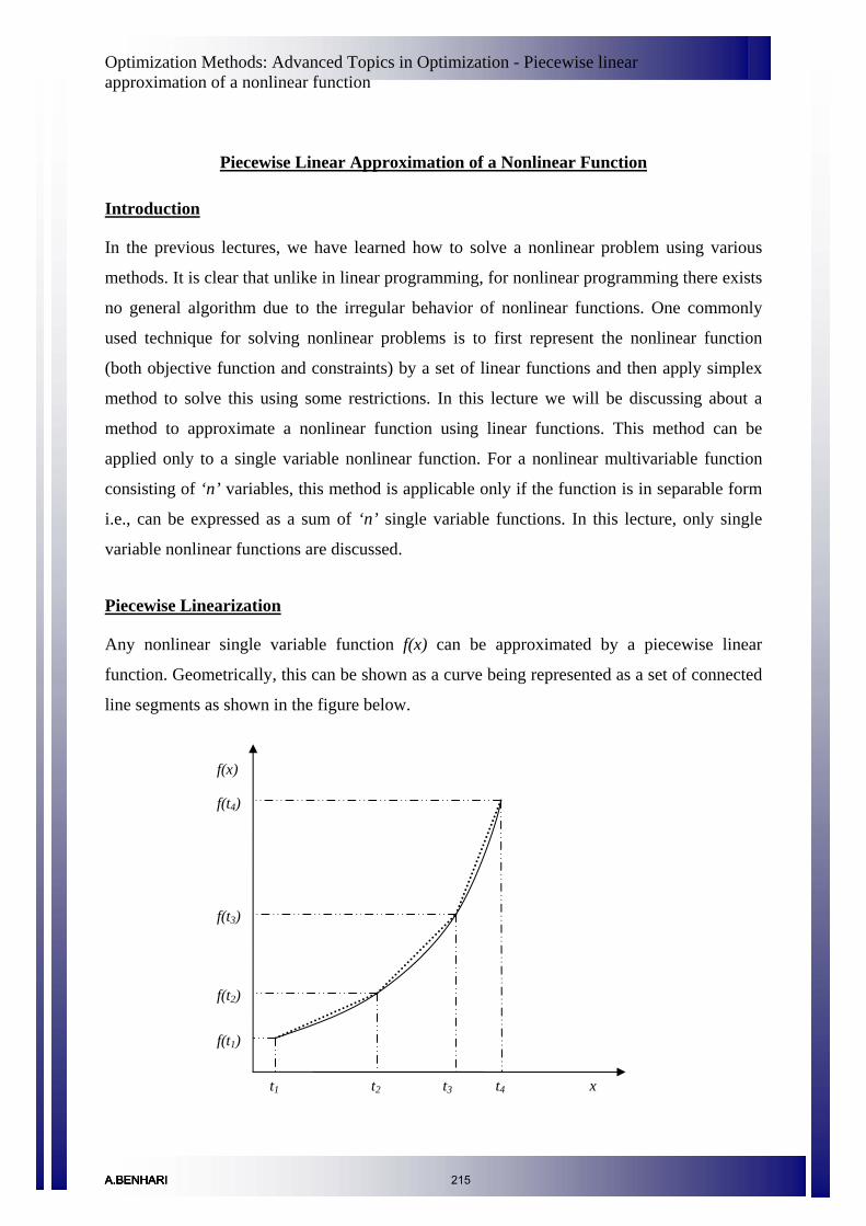
Optimization Methods: Advanced Topics in Optimization - Piecewise linear approximation of a nonlinear function
Piecewise Linear Approximation of a Nonlinear Function
Introduction
In the previous lectures, we have learned how to solve a nonlinear problem using various
methods. It is clear that unlike in linear programming, for nonlinear programming there exists
no general algorithm due to the irregular behavior of nonlinear functions. One commonly
used technique for solving nonlinear problems is to first represent the nonlinear function
(both objective function and constraints) by a set of linear functions and then apply simplex
method to solve this using some restrictions. In this lecture we will be discussing about a
method to approximate a nonlinear function using linear functions. This method can be
applied only to a single variable nonlinear function. For a nonlinear multivariable function
consisting of ‘n’ variables, this method is applicable only if the function is in separable form
i.e., can be expressed as a sum of ‘n’ single variable functions. In this lecture, only single
variable nonlinear functions are discussed.
Piecewise Linearization
Any nonlinear single variable function f(x) can be approximated by a piecewise linear
function. Geometrically, this can be shown as a curve being represented as a set of connected
line segments as shown in the figure below.
t1 t4
f(t4)
f(t3)
f(t2)
f(t1)
x
f(x)
t3t2
A.BENHARIA.BENHARIA.BENHARIA.BENHARI 215
Optimization Methods: Advanced Topics in Optimization - Piecewise linear approximation of a nonlinear function
Method 1:
Consider an optimization function having only one nonlinear term f(x). Let the x-axis of the
nonlinear function f(x) be divided by ‘p’ breaking points t1, t2, t2, …, tp and the corresponding
function values be f(t1), f(t2),…, f(tp). Suppose if ‘x’ can take values in the interval
, then the breaking points can be shown as, Xx ≤≤0
Xttt p ≡<<<≡ ...0 21 .
Expressing ‘x’ as a weighted average of these breaking points,
pptwtwtwx +++= ...2211
∑=
=p
iii twxei
1
.,.
The function f(x) can be expressed as,
( ) ( ) ( ) ( )( )∑
=
=
+++=p
iii
pp
tfw
tfwtfwtfwxf
1
2211 ...
where ∑=
=p
iiw
1
1
Finally the model can be expressed as
Max or Min ( ) ( )∑=
=p
iii tfwxf
1
subject to the additional constraints
∑
∑
=
=
=
=
p
ii
p
iii
w
xtw
1
1
1
Linearly approximated model stated above can be solved using simplex method with some
restrictions. The restricting condition specifies that there should not be more than two ‘wi’ in
the basis and also two ‘wi’ can take positive values only if they are adjacent. This is because,
if the actual value of ‘x’ is between ti and ti+1, then ‘x’ can be represented as a weighted
A.BENHARIA.BENHARIA.BENHARI 216

Optimization Methods: Advanced Topics in Optimization - Piecewise linear approximation of a nonlinear function
average of wi and wi+1 only i.e., 11 +++= iiii twtwx . Therefore, the contributing weights wi and
wi+1 only will be positive, rest all weights be zero.
Similarly for an objective function consisting of ‘n’ variables (‘n’ terms) represented as
Max or Min ( ) ( ) ( ) ( )nn xfxfxfxf +++= ....2211
subjected to ‘m’ constraints
( ) ( ) ( ) mjforbxgxgxg jnnjjj ,...,2,1....2211 =≤+++
The linear approximation of this problem is
nkforw
mjforbtgwtosubjected
tfwMinorMax
p
iki
j
n
k
p
ikikjki
n
k
p
ikikki
,...,2,11
,...,2,1)(
)(
1
1 1
1 1
==
=≤
∑
∑∑
∑∑
=
= =
= =
Method 2:
Let ‘x’ be expressed as a sum, instead of expressing as the weighted sum of the breaking
points as in the previous method. Then,
∑−
=
−
+=
++++=1
11
1211 ....p
ii
p
ut
uuutx
where is the increment of the variable ‘x’ in the interval , i.e., the bound of is iu ),( 1+ii tt iu
iii ttu −≤≤ +10 .
The function f(x) can be expressed as
( ) ( ) i
p
iiutfxf ∑
−
=
+=1
11 α
where iα represents the slope of the linear approximation between the points and
given by
1+it it
A.BENHARIA.BENHARIA.BENHARI 217
Optimization Methods: Advanced Topics in Optimization - Piecewise linear approximation of a nonlinear function
( ) ( )ii
iii tt
tftf−−
=+
+
1
1α .
Finally the model can be expressed as
Max or Min ( ) ( ) i
p
iiutfxf ∑
−
=
+=1
11 α
subjected to the additional constraints
1,....,2,1,0 1
1
11
−=−≤≤
=+
+
−
=∑
pittu
xut
iii
p
ii
Example
The example below illustrates the application of method 1.
Consider the objective function
Maximize 231 xxf +=
subject to
0
401522
2
1
221
≥≤≤
≤+
xx
xx
The problem is already in separable form (i.e., each term consists of only one variable). So
we can split up the objective function and constraint into two parts
( ) ( )( ) ( )2121111
2211
xgxggxfxff
+=+=
where
( ) ( )( ) ( ) 2212
21111
2223111
2;2
;
xxgxxg
xxfxxf
==
==
Since and are in linear form, they are left as such and therefore is treated
as a linear variable. Consider five breaking points for .
( )22 xf ( )212 xg 2x
1x
A.BENHARIA.BENHARIA.BENHARI 218

Optimization Methods: Advanced Topics in Optimization - Piecewise linear approximation of a nonlinear function
Table 1
i it1 ( )ii tf 1 ( )ii tg 11 1 0 0 0 2 1 1 2 3 2 8 8 4 3 27 18 5 4 64 32
Thus, can be written as, ( )11 xf
( ) ( )
6427810 1514131211
5
111111
×+×+×+×+×=
=∑=
wwwww
tfwxfi
ii
and can be written as, ( )111 xg
( ) ( )
3218820 1514131211
5
1111111
×+×+×+×+×=
=∑=
wwwww
tgwxgi
iii
The linear approximation of the above problem thus becomes,
Maximize 215141312 64278 xwwwwf ++++=
subject to
5,...,2,101
152321882
1
1514131211
1215141312
=≥=++++
=+++++
iforwwwwww
sxwwww
i
This can be solved using simplex method in a restricted basis condition.
Table 2
Variables rb
rs
r
cb
Iteration Basis f
11w 12w 13w 14w 15w 2x 1s
f 1 0 -1 -8 -27 -64 -1 0 0 --
1s 0 0 2 8 18 32 2 1 15 1.87
1
11w 0 1 1 1 1 1 0 0 1 1
A.BENHARIA.BENHARIA.BENHARI 219

Optimization Methods: Advanced Topics in Optimization - Piecewise linear approximation of a nonlinear function
From the table above, it is clear that should be the entering variable. For that should
be the exiting variable. But according to restricted basis condition and cannot occur
together in basis as they are not adjacent. Therefore, consider the next best entering
variable . This also is not possible, since should be exited and and cannot occur
together. Again, considering the next best variable , it is clear that should be the
exiting variable.
15w 1s
15w 11w
14w 1s 14w 11w
13w 11w
Table 3
Variables rb
rs
r
cb
Iteration Basis f
11w 12w 13w 14w 15w 2x 1s
f 1 8 7 0 -19 -56 1 0 8 --
1s 0 -8 -6 0 10 24 2 1 7 3
1
13w 0 1 1 1 1 1 0 0 1 15
For the table 2 above, the entering variable is . Then the variable to be exited is and this
is not acceptable since is not an adjacent point to . Next variable can be admitted
by dropping .
15w 1s
15w 13w 14w
1s
Table 4
Variables rb
rs
r
cb
Iteration Basis f
11w 12w 13w 14w 15w 2x 1s
f 1 -7.2 -4.4 0 0 -10.4 4.8 1.9 21.3 --
14w 0 -0.8 -0.6 0 1 2.4 0.2 0.1 0.7 1
13w 0 1.8 1.6 1 0 -1.4 -0.2 -0.1 0.3
A.BENHARIA.BENHARIA.BENHARI 220

Optimization Methods: Advanced Topics in Optimization - Piecewise linear approximation of a nonlinear function
Now, cannot be admitted since cannot be dropped. Similarly and cannot be
entered as cannot be dropped. Thus, the process ends at this point and the last table gives
the best solution.
15w 14w 11w 12w
13w
7.0;3.0 1413 == ww
Now,
7.232 1413
5
1111
=×+×=
=∑=
ww
twxi
ii
02 =xand
The optimum value of . 3.21=f
This may be an approximate solution to the original nonlinear problem. However, the
solution can be improved by taking finer breaking points.
A.BENHARIA.BENHARIA.BENHARI 221
Optimization Methods: Advanced Topics in Optimization - Multi-objective Optimization
Multi-objective Optimization
Introduction
In a real world problem it is very unlikely that we will meet the situation of single objective
and multiple constraints more often than not. Thus the rigidity provided by the General
Problem (GP) is, many a times, far away from the practical design problems. In many of the
water resources optimization problems maximizing aggregated net benefits is a common
objective. At the same time maximizing water quality, regional development, resource
utilization, and various social issues are other objectives which are to be maximized. There
may be conflicting objectives along with the main objective like irrigation, hydropower,
recreation etc. Generally multiple objectives or parameters have to be met before any
acceptable solution can be obtained. Here it should be noticed that the word “acceptable”
implicates that there is normally no single solution to the problems of the above type.
Actually methods of multi-criteria or multi-objective analysis are not designed to identify the
best solution, but only to provide information on the tradeoffs between given sets of
quantitative performance criteria.
In the present discussion on multi-objective optimization, we will first introduce the
mathematical definition and then talk about two broad classes of solution methods typically
known as (i) Utility Function Method (Weighting function method) (ii) Bounded Objective
Function Method (Reduced Feasible Region Method or Constraint Method ).
Multi-objective Problem
A multi-objective optimization problem with inequality (or equality) constraints may be
formulated as
A.BENHARIA.BENHARIA.BENHARIA.BENHARI 222

Optimization Methods: Advanced Topics in Optimization - Multi-objective Optimization
Find (1)
⎪⎪⎪⎪
⎭
⎪⎪⎪⎪
⎬
⎫
⎪⎪⎪⎪
⎩
⎪⎪⎪⎪
⎨
⎧
=
nx
xx
X
.
.
.2
1
which minimizes f1(X), f2(X), … , fk(X) (2)
subject to
j= 1, 2 , … , m (3) ,0)( ≤Xg j
Here k denotes the number of objective functions to be minimized and m is the number of
constraints. It is worthwhile to mention that objective functions and constraints need not be
linear but when they are, it is called Multi-objective Linear Programming (MOLP).
For the problems of the type mentioned above the very notion of optimization changes and
we try to find good trade-offs rather than a single solution as in GP. The most commonly
adopted notion of the “optimum” proposed by Pareto is depicted below.
A vector of the decision variable X is called Pareto Optimal (efficient) if there does not exist
another Y such that for i = 1, 2, … , k with )()( XfYf ii ≤ )()( XfYf ij < for at least one j. In
other words a solution vector X is called optimal if there is no other vector Y that reduces
some objective functions without causing simultaneous increase in at least one other
objective function.
A.BENHARIA.BENHARIA.BENHARI 223

Optimization Methods: Advanced Topics in Optimization - Multi-objective Optimization
k
ij
Fig. 1
As shown in above figure there are three objectives i, j, k. Direction of their increment is also
indicated. The surface (which is formed based on constraints) is efficient because no
objective can be reduced without a simultaneous increase in at least one of the other
objectives.
Utility Function Method (Weighting function method)
In this method a utility function is defined for each of the objectives according to the relative
importance of fi.. A simple utility function may be defined as αifi(X) for ith objective where αi
is a scalar and represents the weight assigned to the corresponding objective. Then the total
utility U may be defined as weighted sum of objective functions as below
U = α,)(1∑=
k
iii Xfα i > 0, i = 1, 2, … , k. (4)
The solution vector X may be found by maximizing the total utility as defined above with the
constraint (3).
Without any loss to generality, it is customary to assume that although it is not
essential. Also α
11
=∑=
k
iiα
i values indicate the relative utility of each of the objectives.
A.BENHARIA.BENHARIA.BENHARI 224
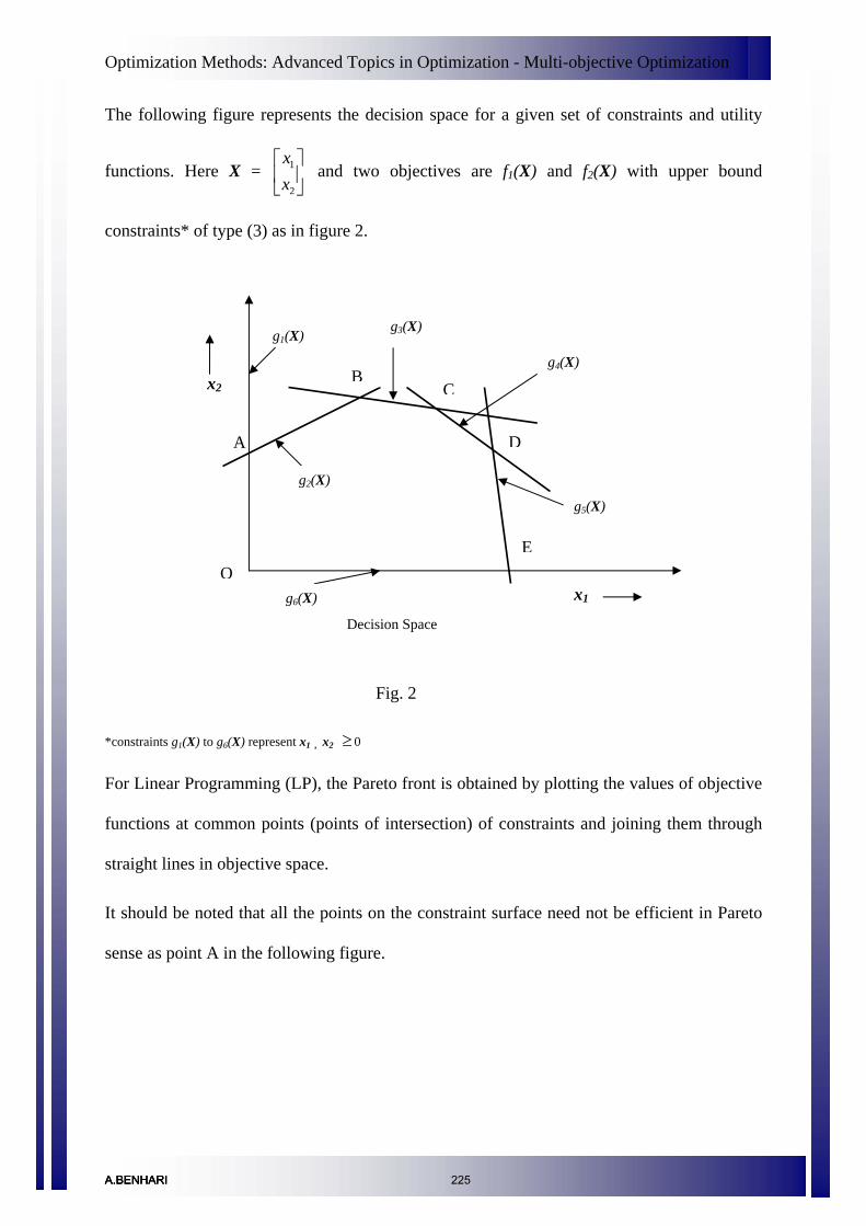
Optimization Methods: Advanced Topics in Optimization - Multi-objective Optimization
The following figure represents the decision space for a given set of constraints and utility
functions. Here X = and two objectives are f⎥⎦
⎤⎢⎣
⎡
2
1
xx
1(X) and f2(X) with upper bound
constraints* of type (3) as in figure 2.
g1(X)
g2(X)
g3(X)
g4(X)
g5(X)
g6(X)
x2
A
BC
D
EO
x1
Decision Space
Fig. 2
*constraints g1(X) to g6(X) represent x1 , x2 ≥ 0
For Linear Programming (LP), the Pareto front is obtained by plotting the values of objective
functions at common points (points of intersection) of constraints and joining them through
straight lines in objective space.
It should be noted that all the points on the constraint surface need not be efficient in Pareto
sense as point A in the following figure.
A.BENHARIA.BENHARIA.BENHARI 225

Optimization Methods: Advanced Topics in Optimization - Multi-objective Optimization
A
BC
D
E
f2
f1
Objective Space
Fig. 3
By looking at Figure 3 one may qualitatively infer that it follows Pareto Optimal definition.
Now optimizing utility function means moving along the efficient front and looking for the
maximum value of utility function U defined by equation (4).
One major limitation is that this method cannot generate the complete set of efficient
solutions unless the efficiency frontier is strictly convex. If a part of it is concave, only the
end points of this can be obtained by the weighing technique.
Bounded objective function method
In this method we try to trap the optimal solution of the objective functions in a bounded or
reduced feasible region. In formulating the problem one objective function is maximized
while all other objectives are converted into constraints with lower bounds along with other
constraints of the problem. Mathematically the problem may be formulated as
Maximize fi(X)
Subject to ,0)( ≤Xg j j= 1, 2 , … , m (5)
A.BENHARIA.BENHARIA.BENHARI 226

Optimization Methods: Advanced Topics in Optimization - Multi-objective Optimization
fk(X) e≥ k ∀ ik ≠
here ek represents lower bound of the kth objective. In this approach the feasible region S
represented by ,0)( ≤Xg j j= 1, 2 , … , m is further reduced to S’ by (k-1) constraints
fk(X) e≥ k . ∀ ik ≠
e.g. let there are three objectives which are to be maximized in the region of constraints S.
The problem may be formulated as:
maximize{objective-1}
maximize{objective-2}
maximize{objective-3}
subject to X = ⎥⎦
⎤⎢⎣
⎡
2
1
xx
∈ S
In the above problem S identifies the region given by ,0)( ≤Xg j j= 1, 2 , … , m.
In the bounded objective function method, the same problem may be formulated as
maximize{objective-1}
subject to
{objective-2} e≥ 1
{objective-3} e≥ 2
X ∈ S
As may be seen, one of the objectives ({objective-1}) is now the only objective and all other
objectives are included as constraints. There are lower bounds specified for other objectives
which are the minimum values at least to be attained. Subject to these additional constraints,
the objective is maximized. Figure 4 illustrates the scheme.
A.BENHARIA.BENHARIA.BENHARI 227

Optimization Methods: Advanced Topics in Optimization - Multi-objective Optimization
x2
w1
w2
w3
S
S’A
BC
D
Ee1
e2P
x1F
Fig. 4
In the above figure w1, w2, and w3 are gradients of the three objectives respectively. If
{objective-1} was to be maximized in the region S, without taking into consideration the
other objectives, then solution point is E. But due to lower bounds of the other objectives the
feasible region reduces to S’ and solution point is P now. It may be seen that changing e1
does not affect {objective-1} as much as changing e2. This fact gives rise to sensitivity
analysis.
Exercise Problem
A reservoir is planned both for gravity and lift irrigation through withdrawals from its
storage. The total storage available for both the uses is limited to 5 units each year. It is
decided to limit the gravity irrigation withdrawals in a year to 4 units. If X1 is the allocation
of water for gravity irrigation and X2 is the allocation for lift irrigation, the two objectives
planned to be maximized are expressed as
Maximize Z1(X) = 3x1 - 2x2 and Z2(X) = - x1 + 4x2
A.BENHARIA.BENHARIA.BENHARI 228

Optimization Methods: Advanced Topics in Optimization - Multi-objective Optimization
For above problem, do the following
(i) Generate a Pareto Front of non-inferior (efficient) solutions by plotting Decision space and
Objective space.
(ii) Formulate multi objective optimization model using weighting approach with w1 and w2
as weights for gravity and lift irrigation respectively.
(iii) Solve it, for (i) w1=1 and w2=2 (ii) w1=2 and w2=1
(iv) Formulate the problem using constraint method
[Solution: (i) X1=0, X2=5; (ii) X1=4, X2=0 to 1 ]
A.BENHARIA.BENHARIA.BENHARI 229
Optimization Methods: Advanced Topics in Optimization - Multilevel Optimization
Multilevel Optimization
Introduction
The example problems discussed in the previous modules consist of very few decision
variables and constraints. However in practical situations, one has to handle an optimization
problem involving a large number of variables and constraints. Solving such a problem will
be quite cumbersome. In multilevel optimization, such large sized problems are decomposed
into smaller independent problems and the overall optimum solution can be obtained by
solving each sub-problem independently. In this lecture a decomposition method for
nonlinear optimization problems, known as model-coordination method will be discussed.
Model Coordination Method
Consider a minimization optimization problem consisting of n variables, . )(xF nxxx ,...,, 21
),...,,( 21 nxxxFMin
subjected to constraints
niuxxlx
mjxxxg
iii
nj
,...,2,1
,...,2,1,0),...,,( 21
=≤≤
=≤
where and represents the lower and upper bounds of the decision variable . ilx iux ix
Let be the decision variable vector. For applying the model coordination
method, the vector X should be divided into two subvectors, Y and Z such that Y contains the
coordination variables between the subsystems i.e., variables that are common to the
subproblems and Z vector contains the free or confined variables of subproblems. If the
problem is partitioned into ‘P’ subproblems, then vector Z can also be partitioned into ‘P’
variable sets, each set corresponding to each subproblem.
{ nxxxX ,...,, 21= }
⎪⎪⎭
⎪⎪⎬
⎫
⎪⎪⎩
⎪⎪⎨
⎧
=
PZ
ZZ
ZM
2
1
Thus the objective function can be partitioned into ‘P’ parts as shown, )(xF
A.BENHARIA.BENHARIA.BENHARIA.BENHARI 230
Optimization Methods: Advanced Topics in Optimization - Multilevel Optimization
( )∑=
=P
kkk ZYfxF
1,)(
where denotes the objective function of the k( kk ZYf , ) th subproblem. In this the coordination
variable Y will appear in all sub-objective functions and will appear only in kkZ th sub-
objective function.
Similarly the constraints can be decomposed as
PkforZYg kk ,...,2,10),( =≤
The lower and upper bound constraints are
PkforuZZlZuYYlY
kkk ,...,2,1=≤≤≤≤
The problem thus decomposed is solved using a two level approach which is described
below.
Procedure:
First level:
Fix the value of the coordination variables, Y at some value, say . Then solve each
independent subproblem and find the value of .
optY
kZ
( )kk ZYfMin ,
subject to
PkforuZZlZuYYlY
ZYg
kkk
kk
,...,2,1
0),(
=≤≤≤≤
≤
Let the values of obtained by solving this problem be . kZ optkZ
Second level:
Now consider the problem after substituting the values. optkZ
( )∑=
=P
koptkk ZYfYfMin
1,)(
subject to uYYlY ≤≤
A.BENHARIA.BENHARIA.BENHARI 231

Optimization Methods: Advanced Topics in Optimization - Multilevel Optimization
Solve this problem to find a new . Again solve the first level problems. This process is
repeated until convergence is achieved.
optY
A.BENHARIA.BENHARIA.BENHARI 232
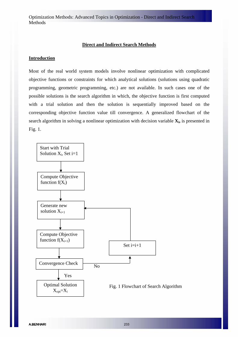
Optimization Methods: Advanced Topics in Optimization - Direct and Indirect Search Methods
Direct and Indirect Search Methods
Introduction
Most of the real world system models involve nonlinear optimization with complicated
objective functions or constraints for which analytical solutions (solutions using quadratic
programming, geometric programming, etc.) are not available. In such cases one of the
possible solutions is the search algorithm in which, the objective function is first computed
with a trial solution and then the solution is sequentially improved based on the
corresponding objective function value till convergence. A generalized flowchart of the
search algorithm in solving a nonlinear optimization with decision variable Xi, is presented in
Fig. 1.
Fig. 1 Flowchart of Search Algorithm
No
Start with Trial Solution Xi, Set i=1
Compute Objective function f(Xi)
Generate new solution Xi+1
Compute Objective function f(Xi+1)
Convergence Check
Set i=i+1
Optimal Solution Xopt=Xi
Yes
A.BENHARIA.BENHARIA.BENHARIA.BENHARI 233

Optimization Methods: Advanced Topics in Optimization - Direct and Indirect Search Methods
The search algorithms can be broadly classified into two types: (1) direct search algorithm
and (2) indirect search algorithm. A direct search algorithm for numerical search optimization
depends on the objective function only through ranking a countable set of function values. It
does not involve the partial derivatives of the function and hence it is also called nongradient
or zeroth order method. Indirect search algorithm, also called the descent method, depends on
the first (first-order methods) and often second derivatives (second-order methods) of the
objective function. A brief overview of the direct search algorithm is presented.
Direct Search Algorithm
Some of the direct search algorithms for solving nonlinear optimization, which requires
objective functions, are described below:
A) Random Search Method: This method generates trial solutions for the optimization model
using random number generators for the decision variables. Random search method includes
random jump method, random walk method and random walk method with direction
exploitation. Random jump method generates huge number of data points for the decision
variable assuming a uniform distribution for them and finds out the best solution by
comparing the corresponding objective function values. Random walk method generates trial
solution with sequential improvements which is governed by a scalar step length and a unit
random vector. The random walk method with direct exploitation is an improved version of
random walk method, in which, first the successful direction of generating trial solutions is
found out and then maximum possible steps are taken along this successful direction.
B) Grid Search Method: This methodology involves setting up of grids in the decision space
and evaluating the values of the objective function at each grid point. The point which
corresponds to the best value of the objective function is considered to be the optimum
solution. A major drawback of this methodology is that the number of grid points increases
exponentially with the number of decision variables, which makes the method
computationally costlier.
C) Univariate Method: This procedure involves generation of trial solutions for one decision
variable at a time, keeping all the others fixed. Thus the best solution for a decision variable
A.BENHARIA.BENHARIA.BENHARI 234
Optimization Methods: Advanced Topics in Optimization - Direct and Indirect Search Methods
keeping others constant can be obtained. After completion of the process with all the decision
variables, the algorithm is repeated till convergence.
D) Pattern Directions: In univariate method the search direction is along the direction of co-
ordinate axis which makes the rate of convergence very slow. To overcome this drawback,
the method of pattern direction is used, in which, the search is performed not along the
direction of the co-ordinate axes but along the direction towards the best solution. This can be
achieved with Hooke and Jeeves’ method or Powell’s method. In the Hooke and Jeeves’
method, a sequential technique is used consisting of two moves: exploratory move and the
pattern move. Exploratory move is used to explore the local behavior of the objective
function, and the pattern move is used to take advantage of the pattern direction. Powell’s
method is a direct search method with conjugate gradient, which minimizes the quadratic
function in a finite number of steps. Since a general nonlinear function can be approximated
reasonably well by a quadratic function, conjugate gradient minimizes the computational time
to convergence.
E)Rosen Brock’s Method of Rotating Coordinates: This is a modified version of Hooke and
Jeeves’ method, in which, the coordinate system is rotated in such a way that the first axis
always orients to the locally estimated direction of the best solution and all the axes are made
mutually orthogonal and normal to the first one.
F) Simplex Method: Simplex method is a conventional direct search algorithm where the best
solution lies on the vertices of a geometric figure in N-dimensional space made of a set of
N+1 points. The method compares the objective function values at the N+1 vertices and
moves towards the optimum point iteratively. The movement of the simplex algorithm is
achieved by reflection, contraction and expansion.
Indirect Search Algorithm
The indirect search algorithms are based on the derivatives or gradients of the objective
function. The gradient of a function in N-dimensional space is given by:
A.BENHARIA.BENHARIA.BENHARI 235

Optimization Methods: Advanced Topics in Optimization - Direct and Indirect Search Methods
⎥⎥⎥⎥⎥⎥⎥⎥⎥
⎦
⎤
⎢⎢⎢⎢⎢⎢⎢⎢⎢
⎣
⎡
∂∂
∂∂
∂∂
=∇
Nxf
xf
xf
f
.
.
.2
1
(1)
Indirect search algorithms include:
A) Steepest Descent (Cauchy) Method: In this method, the search starts from an initial trial
point X1, and iteratively moves along the steepest descent directions until the optimum point
is found. Although, the method is straightforward, it is not applicable to the problems having
multiple local optima. In such cases the solution may get stuck at local optimum points.
B) Conjugate Gradient (Fletcher-Reeves) Method: The convergence technique of the steepest
descent method can be greatly improved by using the concept of conjugate gradient with the
use of the property of quadratic convergence.
C) Newton’s Method: Newton’s method is a very popular method which is based on Taylor’s
series expansion. The Taylor’s series expansion of a function f(X) at X=Xi is given by:
( ) ( ) ( ) ( ) [ ]( iiT
iiT
ii XXJXXXXfXfXf −−+−∇+=21 ) (2)
where, [Ji]=[J]|xi , is the Hessian matrix of f evaluated at the point Xi. Setting the partial
derivatives of Eq. (2), to zero, the minimum value of f(X) can be obtained.
( ) NjxXf
j
,...,2,1,0 ==∂∂ (3)
A.BENHARIA.BENHARIA.BENHARI 236

Optimization Methods: Advanced Topics in Optimization - Direct and Indirect Search Methods
From Eq. (2) and (3)
[ ]( ) 0=−+∇=∇ iii XXJff (4)
Eq. (4) can be solved to obtain an improved solution Xi+1
[ ] iiii fJXX ∇−= −+
11 (5)
The procedure is repeated till convergence for finding out the optimal solution.
D) Marquardt Method: Marquardt method is a combination method of both the steepest
descent algorithm and Newton’s method, which has the advantages of both the methods,
movement of function value towards optimum point and fast convergence rate. By modifying
the diagonal elements of the Hessian matrix iteratively, the optimum solution is obtained in
this method.
E) Quasi-Newton Method: Quasi-Newton methods are well-known algorithms for finding
maxima and minima of nonlinear functions. They are based on Newton's method, but they
approximate the Hessian matrix, or its inverse, in order to reduce the amount of computation
per iteration. The Hessian matrix is updated using the secant equation, a generalization of the
secant method for multidimensional problems.
It should be noted that the above mentioned algorithms can be used for solving only
unconstrained optimization. For solving constrained optimization, a common procedure is the
use of a penalty function to convert the constrained optimization problem into an
unconstrained optimization problem. Let us assume that for a point Xi, the amount of
violation of a constraint is δ. In such cases the objective function is given by:
( ) ( ) 2δλ ××+= MXfXf ii (6)
where, λ=1( for minimization problem) and -1 ( for maximization problem), M=dummy
variable with a very high value. The penalty function automatically makes the solution
inferior where there is a violation of constraint.
A.BENHARIA.BENHARIA.BENHARI 237

Optimization Methods: Advanced Topics in Optimization - Direct and Indirect Search Methods
Summary
Various methods for direct and indirect search algorithms are discussed briefly in the present
class. The models are useful when no analytical solution is available for an optimization
problem. It should be noted that when there is availability of an analytical solution, the search
algorithms should not be used, because analytical solution gives a global optima whereas,
there is always a possibility that the numerical solution may get stuck at local optima.
A.BENHARIA.BENHARIA.BENHARI 238

Optimization Methods: Advanced Topics in Optimization - Evolutionary Algorithms for Optimization and Search
Evolutionary Algorithms for Optimization and Search
Introduction
Most real world optimization problems involve complexities like discrete, continuous or
mixed variables, multiple conflicting objectives, non-linearity, discontinuity and non-convex
region. The search space (design space) may be so large that global optimum cannot be found
in a reasonable time. The existing linear or nonlinear methods may not be efficient or
computationally inexpensive for solving such problems. Various stochastic search methods
like simulated annealing, evolutionary algorithms (EA) or hill climbing can be used in such
situations. EAs have the advantage of being applicable to any combination of complexities
(multi-objective, non-linearity etc) and also can be combined with any existing local search
or other methods. Various techniques which make use of EA approach are Genetic
Algorithms (GA), evolutionary programming, evolution strategy, learning classifier system
etc. All these EA techniques operate mainly on a population search basis. In this lecture
Genetic Algorithms, the most popular EA technique, is explained.
Concept
EAs start from a population of possible solutions (called individuals) and move towards the
optimal one by applying the principle of Darwinian evolution theory i.e., survival of the
fittest. Objects forming possible solution sets to the original problem is called phenotype and
the encoding (representation) of the individuals in the EA is called genotype. The mapping of
phenotype to genotype differs in each EA technique. In GA which is the most popular EA,
the variables are represented as strings of numbers (normally binary). If each design variable
is given a string of length ‘l’, and there are n such variables, then the design vector will have
a total string length of ‘nl’. For example, let there are 3 design variables and the string length
be 4 for each variable. The variables are 17,4 321 === xandxx . Then the chromosome
length is 12 as shown in the figure.
0 1 0 0 0 1 1 1 0 0 0 1
1x 2x 3x
A.BENHARIA.BENHARIA.BENHARIA.BENHARI 239

Optimization Methods: Advanced Topics in Optimization - Evolutionary Algorithms for Optimization and Search
An individual consists a genotype and a fitness function. Fitness represents the quality of the
solution (normally called fitness function). It forms the basis for selecting the individuals and
thereby facilitates improvements.
The pseudo code for a simple EA is given below
i = 0
Initialize population P0 Evaluate initial population
while ( ! termination condition) {
i = i+1
Perform competitive selection
Create population Pi from Pi-1 by recombination and mutation
Evaluate population Pi }
A flowchart indicating the steps of a simple genetic algorithm is shown below.
A.BENHARIA.BENHARIA.BENHARI 240

Optimization Methods: Advanced Topics in Optimization - Evolutionary Algorithms for Optimization and Search
Generate Initial Population
Start
Encode Generated Population
Evaluate Fitness Functions
Meets Optimization
Criteria?
Best Individuals
Yes
Stop
Selection (select parents)
Mutation (mutate offsprings)
Crossover (selected parents)
No
REGENERAT ION
The initial population is usually generated randomly in all EAs. The termination condition
may be a desired fitness function, maximum number of generations etc. In selection,
individuals with better fitness functions from generation ‘i' are taken to generate individuals
of ‘i+1’th generation. New population (offspring) is created by applying recombination and
mutation to the selected individuals (parents). Recombination creates one or two new
individuals by swaping (crossing over) the genome of a parent with another. Recombined
individual is then mutated by changing a single element (genome) to create a new individual.
A.BENHARIA.BENHARIA.BENHARI 241

Optimization Methods: Advanced Topics in Optimization - Evolutionary Algorithms for Optimization and Search
Finally, the new population is evaluated and the process is repeated. Each step is described in
more detail below.
Parent Selection
After fitness function evaluation, individuals are distinguished based on their quality.
According to Darwin's evolution theory the best ones should survive and create new offspring
for the next generation. There are many methods to select the best chromosomes, for example
roulette wheel selection, Boltzman selection, tournament selection, rank selection, steady
state selection and others. Two of these are briefly described, namely, roulette wheel
selection and rank selection:
Roulette Wheel Selection:
Parents are selected according to their fitness i.e., each individual is selected with a
probability proportional to its fitness value. In other words, depending on the percentage
contribution to the total population fitness, string is selected for mating to form the next
generation. This way, weak solutions are eliminated and strong solutions survive to form the
next generation. For example, consider a population containing four strings shown in the
table below. Each string is formed by concatenating four substrings which represents
variables a,b,c and d. Length of each string is taken as four bits. The first column represents
the possible solution in binary form. The second column gives the fitness values of the
decoded strings. The third column gives the percentage contribution of each string to the total
fitness of the population. Then by "Roulette Wheel" method, the probability of candidate 1
being selected as a parent of the next generation is 28.09%. Similarly, the probability that the
candidates 2, 3, 4 will be chosen for the next generation are 19.59, 12.89 and 39.43
respectively. These probabilities are represented on a pie chart, and then four numbers are
randomly generated between 1 and 100. Then, the likeliness that the numbers generated
would fall in the region of candidate 2 might be once, whereas for candidate 4 it might be
twice and candidate 1 more than once and for candidate 3 it may not fall at all. Thus, the
strings are chosen to form the parents of the next generation.
A.BENHARIA.BENHARIA.BENHARI 242
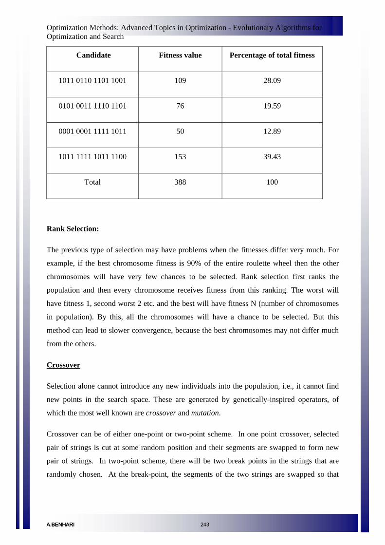
Optimization Methods: Advanced Topics in Optimization - Evolutionary Algorithms for Optimization and Search
Candidate Fitness value Percentage of total fitness
1011 0110 1101 1001 109 28.09
0101 0011 1110 1101 76 19.59
0001 0001 1111 1011 50 12.89
1011 1111 1011 1100 153 39.43
Total 388 100
Rank Selection:
The previous type of selection may have problems when the fitnesses differ very much. For
example, if the best chromosome fitness is 90% of the entire roulette wheel then the other
chromosomes will have very few chances to be selected. Rank selection first ranks the
population and then every chromosome receives fitness from this ranking. The worst will
have fitness 1, second worst 2 etc. and the best will have fitness N (number of chromosomes
in population). By this, all the chromosomes will have a chance to be selected. But this
method can lead to slower convergence, because the best chromosomes may not differ much
from the others.
Crossover
Selection alone cannot introduce any new individuals into the population, i.e., it cannot find
new points in the search space. These are generated by genetically-inspired operators, of
which the most well known are crossover and mutation.
Crossover can be of either one-point or two-point scheme. In one point crossover, selected
pair of strings is cut at some random position and their segments are swapped to form new
pair of strings. In two-point scheme, there will be two break points in the strings that are
randomly chosen. At the break-point, the segments of the two strings are swapped so that
A.BENHARIA.BENHARIA.BENHARI 243

Optimization Methods: Advanced Topics in Optimization - Evolutionary Algorithms for Optimization and Search
new set of strings are formed. For example, let us consider two 8-bit strings given by
'10011101' and '10101011'.
Then according to one-point crossover, if a random crossover point is chosen after 3 bits from
left and segments are cut as shown below:
100 | 11101
101 | 01011
and the segments are swapped to form
10001011
10111101
According to two-point crossover, if two crossover points are selected as
100 | 11 | 101
101 | 01 | 011
Then after swapping both the extreme segments, the resulting strings formed are
10001101
10111011
Crossover is not usually applied to all pairs of individuals selected for mating. A random
choice is made, where the probability of crossover being applied is typically between 0.6 and
0.9.
Mutation
Mutation is applied to each child individually after crossover. It randomly alters each gene
with a small probability (generally not greater than 0.01). It injects a new genetic character
into the chromosome by changing at random a bit in a string depending on the probability of
mutation.
Example: 10111011
A.BENHARIA.BENHARIA.BENHARI 244

Optimization Methods: Advanced Topics in Optimization - Evolutionary Algorithms for Optimization and Search
is mutated as 10111111
It is seen in the above example that the sixth bit '0' is changed to '1'. Thus, in mutation
process, bits are changed from '1' to '0' or '0' to '1' at the randomly chosen position of
randomly selected strings.
Real-coded GAs
As explained earlier, GAs work with a coding of variables i.e., with a discrete search space.
GAs have also been developed to work directly with continuous variables. In these cases,
binary strings are not used. Instead, the variables are directly used. After the creation of
population of random variables, a reproduction operator can be used to select good strings in
the population.
Advantages and Disadvantages of EA:
EA can be efficiently used for highly complex problems with multi-objectivity, non-linearity
etc. It provides not only a single best solution, but the 2nd best, 3rd best and so on as required.
It gives quick approximate solutions. EA methods can very well incorporate with other local
search algorithms.
There are some drawbacks also in using EA techniques. An optimal solution cannot be
ensured on using EA methods, which are usually known as heuristic search methods.
Convergence of EA techniques are problem oriented. Sensitivity analysis should be carried
out to find out the range in which the model is efficient. Also, the implementation of these
techniques requires good programming skill.
A.BENHARIA.BENHARIA.BENHARIA.BENHARI 245

Optimization Methods: Advanced Topics in Optimization - Applications in Civil Engineering
Applications in Civil Engineering
Introduction
In this lecture we will discuss some applications of multiobjective optimization and
evolutionary algorithms in civil engineering.
Water quality management, waste load allocation
Waste Load Allocation (WLA) in streams refers to the determination of required pollutant
treatment levels at a set of point sources of pollution, to ensure that water quality standards
are maintained throughout the stream. The stakeholders involved in a waste load allocation
are the Pollution Control Agency (PCA) and the dischargers (municipal and industrial) who
are discharging waste into the stream. The goals of the PCA are to improve the water quality
throughout the stream whereas that of the dischargers is to reduce the treatment cost of the
pollutants. Therefore a waste load allocation model can be viewed as a multiobjective
optimization model with conflicting objectives. If the fractional removal level of the pollutant
is denoted by x and the concentration of water quality indicator (e.g., Dissolved Oxygen) is
denoted by c, then the following optimization model can be formulated:
cMaximize (1)
xMinimize (2)
)(xfc = (3)
Eq. (3) represents the relationship between the water quality indicator and the fractional
removal levels of the pollutants. It should be noted that the relationship between c and x may
be nonlinear and therefore linear programming may not be applicable. In such cases the
applications of evolutionary algorithm is a possible solution. Interested readers may refer to
Tung and Hathhorn (1989), Sasikumar and Mujumdar (1998), and Mujumdar and Subbarao
(2004).
A.BENHARIA.BENHARIA.BENHARIA.BENHARI 246
Optimization Methods: Advanced Topics in Optimization - Applications in Civil Engineering
Reservoir Operation
In reservoir operation problems, to achieve the best possible performance of the system,
decisions need to be taken on releases and storages over a period of time considering the
variations in inflows and demands. The goals of a multipurpose reservoir operation problem
can be:
A) Flood control
B) Hydropower generation
C) Meeting irrigation demand
D) Maintaining downstream water quality
Therefore deriving the operation policy for a multipurpose reservoir can be considered as a
multiobjective optimization problem. A typical reservoir operation problem is characterized
by the uncertainty resulting from the random behavior of inflow and demand, incorporation
of which in terms of risk may lead to a nonlinear optimization problem. Application of
evolutionary algorithms is a possible solution for such problems. Interested readers may refer
to Janga Reddy and Nagesh Kumar (2007), Nagesh Kumar and Janga Reddy (2007).
Water Distribution Systems
The typical goals of water distribution systems problem in designing urban pipe system can
be:
A) Meeting the household demands.
B) Minimizing cost of pipe system.
C) Meeting the required water pressure at all nodes of the distribution system.
D) Optimal positioning of valves.
Therefore designing urban water distribution system is a multiobjective problem, which is
also characterized by nonlinearity resulting from the simulation model (e.g., Hardy Cross
method). Multiobjective techniques with search algorithm or evolutionary algorithm are
therefore used for solving such problems. Apart from these, determination of optimum
A.BENHARIA.BENHARIA.BENHARI 247

Optimization Methods: Advanced Topics in Optimization - Applications in Civil Engineering
dosage of chlorine is also another important problem which is highly nonlinear because of the
nonlinear water quality simulation model. Evolutionary algorithms are successfully applied
for such problem in various case studies by different researchers.
Transportation Engineering
Evolutionary algorithm has become a useful tool for solving many problems in transportation
systems engineering. The problem, to efficiently move empty or laden containers for a
logistic company or Truck and Trailer Vehicle Routing Problem (TTVRP), is one among the
many potential research problems in transportation systems engineering. A general model for
TTVRP, consisting of a number of job orders to be served by trucks and trailers daily, is
constructed for a logistic company that provides transportation services for container
movement within the country. Due to the limited capacity of vehicles owned by the company,
the engineers of the company have to decide whether to assign the job orders of container
movement to its internal fleet of vehicles or to outsource the jobs to
other companies. The solution to the TTVRP consists of finding a complete routing schedule
for serving the jobs with - 1. minimum routing distance and 2. minimum number of trucks,
subject to a number of constraints such as time windows and availability of trailers.
Multiobjective evolutionary algorithm can be used to solve such models. Applications of
evolutionary algorithm in solving transportation problems can be found in Lee et al. (2003).
A.BENHARIA.BENHARIA.BENHARIA.BENHARI 248

References :
1. Hillier F.S. and G.J. Lieberman, Operations Research, CBS Publishers & Distributors,
New Delhi, 1987.
2. D.G.Luenberger, Linear and Non-linear Programming. New York:Addison-Wesley,1990.
3. D.E.Goldberg, Genetic algorithms in Search, Optimization, and Machine Learning
NewYork: Addison Wesley Longman,1989.
4. Rao S.S., Engineering Optimization – Theory and Practice, Third Edition, New Age
International Limited, New Delhi, 2000
5. Ravindran A., D.T. Phillips and J.J. Solberg, Operations Research – Principles and
Practice, John Wiley & Sons, New York, 2001.
6. Taha H.A., Operations Research – An Introduction, Prentice-Hall of India Pvt. Ltd., New
Delhi, 2005.
7. Deb K., Multi-Objective Optimization using Evolutionary Algorithms, First Edition, John
Wiley & Sons Pte Ltd, 2002.
8. Deb K., Optimization for Engineering Design – Algorithms and Examples, Prentice Hall
of India Pvt. Ltd., New Delhi, 1995.
9. Dorigo M., and T. Stutzle, Ant Colony Optimization, Prentice Hall of India Pvt. Ltd.,
New Delhi, 2005.
10. Jain S.K. and V.P. Singh, Water Resources Systems Planning and Management, Elsevier
B.V., The Netherlands, 2003.
11. Loucks, D.P., J.R. Stedinger, and D.A. Haith, Water Resources Systems Planning and
Analysis, Prentice – Hall, N.J., 1981.
12. Mays, L.W. and K. Tung, Hydrosystems Engineering and Management, McGraw-Hill
Inc., New York, 1992.
13. Vedula S., and P.P. Mujumdar, Water Resources Systems: Modelling Techniques and
Analysis, Tata McGraw Hill, New Delhi, 2005. A.
14. M.S.Bazaraa, J.J.Jarvis, and H.D.Sherali, Linear Programming and Network Flows
,2nded. New York:JohnWiley&Sons,1990.
15. M.S.Bazaraa, H.D.Sherali, and C.M.Shetty, Nonlinear Programming–theory and algorithms.
NewYork:JohnWiley&Sons,1993.
16. Z.MichalewiczandM.Michalewicz, “Evolutionary computation techniques and their
applications,” in IEEE—International Conference on Intelligent Processing Systems
,Beijing,1997,pp.14–25.
17. P.G.Alotto,C.Eranda,and B.Brandstaetter,“Stochastic algorithms in electromagnetic
optimization,” IEEE Transactions on Magnetics,vol.34,no.5,pp.3674–3684,Sept.1998.
18. C.A.C.Coello, “Handling preferences in evolutionary multiobjective optimization:
A survey,”in IEEE—Congress on Evolutionary Computation,vol.1,New Jersey,2000,pp.30–
37.
19. J.A.VasconcelosandA.H.F.Dias, “Multiobjective genetic algorithms Applied to solve
optimization problems,”IEEE Transactions on Magnetics,vol.38,no.2,pp.1133––
1136,Mar.2002.
20. K.KrishnakumarandD.E.Goldberg,“Control system optimization,” Journal of
Guidance,Control,and Dynamics,vol.15,no.3,pp.735–740,1992.
A.BENHARIA.BENHARIA.BENHARI 249
Top Related