


Languages
Pages
Legal


Lecture Notes1
Mathematical Ecnomics
Guoqiang TIAN
Department of Economics
Texas A&M University
College Station, Texas 77843
This version: September, 2021
1These notes draw heavily upon Chiang’s classic textbook Fundamental Methods ofMathematical Economics and Vinogradov’s notes A Cook-Book of Mathematics, which areused for my teaching and convenience of my students in class. Please not distribute it toany others.
Contents
1 The Nature of Mathematical Economics 1
1.1 Economics and Mathematical Economics . . . . . . . . . . . 1
1.2 Advantages of Mathematical Approach . . . . . . . . . . . . 2
1.3 Scientific Analytic Methods: Three Dimensions and Six Na-
tures . . . . . . . . . . . . . . . . . . . . . . . . . . . . . . . . 3
2 Economic Models 5
2.1 Ingredients of a Mathematical Model . . . . . . . . . . . . . . 5
2.2 The Real-Number System . . . . . . . . . . . . . . . . . . . . 5
2.3 The Concept of Sets . . . . . . . . . . . . . . . . . . . . . . . . 6
2.4 Relations and Functions . . . . . . . . . . . . . . . . . . . . . 9
2.5 Types of Function . . . . . . . . . . . . . . . . . . . . . . . . . 11
2.6 Functions of Two or More Independent Variables . . . . . . . 12
2.7 Levels of Generality . . . . . . . . . . . . . . . . . . . . . . . . 13
3 Equilibrium Analysis in Economics 15
3.1 The Meaning of Equilibrium . . . . . . . . . . . . . . . . . . . 15
3.2 Partial Market Equilibrium - A Linear Model . . . . . . . . . 16
3.3 Partial Market Equilibrium - A Nonlinear Model . . . . . . . 18
3.4 General Market Equilibrium . . . . . . . . . . . . . . . . . . . 19
3.5 Equilibrium in National-Income Analysis . . . . . . . . . . . 23
i

ii CONTENTS
4 Linear Models and Matrix Algebra 25
4.1 Matrix and Vectors . . . . . . . . . . . . . . . . . . . . . . . . 26
4.2 Matrix Operations . . . . . . . . . . . . . . . . . . . . . . . . . 29
4.3 Linear Dependance of Vectors . . . . . . . . . . . . . . . . . . 32
4.4 Commutative, Associative, and Distributive Laws . . . . . . 33
4.5 Identity Matrices and Null Matrices . . . . . . . . . . . . . . 35
4.6 Transposes and Inverses . . . . . . . . . . . . . . . . . . . . . 36
5 Linear Models and Matrix Algebra (Continued) 41
5.1 Conditions for Nonsingularity of a Matrix . . . . . . . . . . . 41
5.2 Test of Nonsingularity by Use of Determinant . . . . . . . . . 43
5.3 Basic Properties of Determinants . . . . . . . . . . . . . . . . 49
5.4 Finding the Inverse Matrix . . . . . . . . . . . . . . . . . . . . 54
5.5 Cramer’s Rule . . . . . . . . . . . . . . . . . . . . . . . . . . . 60
5.6 Application to Market and National-Income Models . . . . . 65
5.7 Quadratic Forms . . . . . . . . . . . . . . . . . . . . . . . . . 68
5.8 Eigenvalues and Eigenvectors . . . . . . . . . . . . . . . . . . 72
5.9 Vector Spaces . . . . . . . . . . . . . . . . . . . . . . . . . . . 75
6 Comparative Statics and the Concept of Derivative 83
6.1 The Nature of Comparative Statics . . . . . . . . . . . . . . . 83
6.2 Rate of Change and the Derivative . . . . . . . . . . . . . . . 84
6.3 The Derivative and the Slope of a Curve . . . . . . . . . . . . 86
6.4 The Concept of Limit . . . . . . . . . . . . . . . . . . . . . . . 87
6.5 Inequality and Absolute Values . . . . . . . . . . . . . . . . . 90
6.6 Limit Theorems . . . . . . . . . . . . . . . . . . . . . . . . . . 92
6.7 Continuity and Differentiability of a Function . . . . . . . . . 93
7 Rules of Differentiation and Their Use in Comparative Statics 97
7.1 Rules of Differentiation for a Function of One Variable . . . . 97

CONTENTS iii
7.2 Rules of Differentiation Involving Two or More Functions
of the Same Variable . . . . . . . . . . . . . . . . . . . . . . . 101
7.3 Rules of Differentiation Involving Functions of Different Vari-
ables . . . . . . . . . . . . . . . . . . . . . . . . . . . . . . . . 107
7.4 Integration (The Case of One Variable) . . . . . . . . . . . . . 110
7.5 Partial Differentiation . . . . . . . . . . . . . . . . . . . . . . . 113
7.6 Applications to Comparative-Static Analysis . . . . . . . . . 115
7.7 Note on Jacobian Determinants . . . . . . . . . . . . . . . . . 118
8 Comparative-Static Analysis of General-Functions 121
8.1 Differentials . . . . . . . . . . . . . . . . . . . . . . . . . . . . 123
8.2 Total Differentials . . . . . . . . . . . . . . . . . . . . . . . . . 127
8.3 Rule of Differentials . . . . . . . . . . . . . . . . . . . . . . . . 128
8.4 Total Derivatives . . . . . . . . . . . . . . . . . . . . . . . . . 130
8.5 Implicit Function Theorem . . . . . . . . . . . . . . . . . . . . 134
8.6 Comparative Statics of General-Function Models . . . . . . . 140
8.7 Matrix Derivatives . . . . . . . . . . . . . . . . . . . . . . . . 141
9 Optimization: Maxima and Minima of a Function of One Vari-
able 143
9.1 Optimal Values and Extreme Values . . . . . . . . . . . . . . 144
9.2 Existence of Extremum for Continuous Function . . . . . . . 145
9.3 First-Derivative Test for Relative Maximum and Minimum . 146
9.4 Second and Higher Derivatives . . . . . . . . . . . . . . . . . 150
9.5 Second-Derivative Test . . . . . . . . . . . . . . . . . . . . . . 151
9.6 Taylor Series . . . . . . . . . . . . . . . . . . . . . . . . . . . . 154
9.7 Nth-Derivative Test . . . . . . . . . . . . . . . . . . . . . . . . 156
10 Exponential and Logarithmic Functions 159
10.1 The Nature of Exponential Functions . . . . . . . . . . . . . . 159

iv CONTENTS
10.2 Logarithmic Functions . . . . . . . . . . . . . . . . . . . . . . 160
10.3 Derivatives of Exponential and Logarithmic Functions . . . 161
11 Optimization: Maxima and Minima of a Function of Two or More
Variables 165
11.1 The Differential Version of Optimization Condition . . . . . 165
11.2 Extreme Values of a Function of Two Variables . . . . . . . . 166
11.3 Objective Functions with More than Two Variables . . . . . . 173
11.4 Second-Order Conditions in Relation to Concavity and Con-
vexity . . . . . . . . . . . . . . . . . . . . . . . . . . . . . . . . 176
11.4.1 Concavity and Convexity . . . . . . . . . . . . . . . . 176
11.4.2 Concavity/Convexity and Global Optimization . . . 182
11.5 Economic Applications . . . . . . . . . . . . . . . . . . . . . . 184
12 Optimization with Equality Constraints 189
12.1 Effects of a Constraint . . . . . . . . . . . . . . . . . . . . . . 190
12.2 Finding the Stationary Values . . . . . . . . . . . . . . . . . . 191
12.3 Second-Order Conditions . . . . . . . . . . . . . . . . . . . . 196
12.4 General Setup of the Problem . . . . . . . . . . . . . . . . . . 200
12.5 Quasiconcavity and Quasiconvexity . . . . . . . . . . . . . . 202
12.6 Utility Maximization and Consumer Demand . . . . . . . . . 209
13 Optimization with Inequality Constraints 213
13.1 Non-Linear Programming . . . . . . . . . . . . . . . . . . . . 214
13.2 Kuhn-Tucker Conditions . . . . . . . . . . . . . . . . . . . . . 215
13.3 Economic Applications . . . . . . . . . . . . . . . . . . . . . . 220
14 Differential Equations 225
14.1 Existence and Uniqueness Theorem of Solutions for Ordi-
nary Differential Equations . . . . . . . . . . . . . . . . . . . 227
CONTENTS v
14.2 Some Common Ordinary Differential Equations with Ex-
plicit Solutions . . . . . . . . . . . . . . . . . . . . . . . . . . . 228
14.3 Higher Order Linear Equations with Constant Coefficients . 232
14.4 System of Ordinary Differential Equations . . . . . . . . . . . 236
14.5 Simultaneous Differential Equations and Stability of Equi-
librium . . . . . . . . . . . . . . . . . . . . . . . . . . . . . . . 241
14.6 The Stability of Dynamical System . . . . . . . . . . . . . . . 243
15 Difference Equations 245
15.1 First-order Difference Equations . . . . . . . . . . . . . . . . 247
15.2 Second-order Difference Equation . . . . . . . . . . . . . . . 250
15.3 Difference Equations of Order n . . . . . . . . . . . . . . . . 251
15.4 The Stability of nth-Order Difference Equations . . . . . . . 253
15.5 Difference Equations with Constant Coefficients . . . . . . . 254
Chapter 1
The Nature of Mathematical
Economics
The purpose of this course is to introduce the most fundamental aspects
of the mathematical methods such as those matrix algebra, mathematical
analysis, and optimization theory.
1.1 Economics and Mathematical Economics
Economics is a social science that studies how to make decisions in face
of scarce resources. Specifically, it studies individuals’ economic behavior
and phenomena as well as how individuals, such as consumers, house-
holds, firms, organizations and government agencies, make trade-off choic-
es that allocate limited resources among competing uses.
Mathematical economics is an approach to economic analysis, in which
the economists make use of mathematical symbols in the statement of the
problem and also draw upon known mathematical theorems to aid in rea-
soning.
Since mathematical economics is merely an approach to economic anal-
1

2 CHAPTER 1. THE NATURE OF MATHEMATICAL ECONOMICS
ysis, it should not and does not differ from the nonmathematical approach
to economic analysis in any fundamental way. The difference between
these two approaches is that in the former, the assumptions and conclu-
sions are stated in mathematical symbols rather than words and in the
equations rather than sentences so that the interdependent relationship
among economic variables and resulting conclusions are more rigorous
and concise by using mathematical models and mathematical statistic-
s/econometric methods.
1.2 Advantages of Mathematical Approach
Mathematical approach has the following advantages:
(1) It makes the language more precise and the statement of as-
sumptions more clear, which can deduce many unnecessary
debates resulting from inaccurate verbal language.
(2) It makes the analytical logic more rigorous and clearly s-
tates the boundary, applicable scope and conditions for a
conclusion to hold. Otherwise, the abuse of a theory may
occur.
(3) Mathematics can help obtain the results that cannot be eas-
ily attained through intuition.
(4) It helps improve and extend the existing economic theories.
It is, however, noteworthy a good master of mathematics cannot guar-
antee to be a good economist. It also requires fully understanding the an-
alytical framework and research methodologies of economics, and having
a good intuition and insight of real economic environments and econom-
ic issues. The study of economics not only calls for the understanding of

1.3. SCIENTIFIC ANALYTIC METHODS: THREE DIMENSIONS AND SIX NATURES3
some terms, concepts and results from the perspective of mathematics (in-
cluding geometry), but more importantly, even when those are given by
mathematical language or geometric figure, we need to get to their eco-
nomic meaning and the underlying profound economic thoughts and ide-
als. Thus we should avoid being confused by the mathematical formulas
or symbols in the study of economics.
1.3 Scientific Analytic Methods: Three Dimen-
sions and Six Natures
Scientific economic analysis, especially aimed at studying and solving ma-
jor practical problems affecting the overall situation, is inseparable from
"three dimensions and six natures”:
Three dimensions: theoretical logic, practical knowledge, and his-
torical perspective;
Six natures: scientific, rigorous, realistic, pertinent, forward-looking
and thought-provoking.
Since social economic issues generally cannot be studied by only using
real society and performing experiments on it, we need not only theo-
retical analysis with inherent logical inferences, but also empirical quan-
titative analysis or tests with appropriate tools, such as statistics and e-
conometrics. However, only using theory and practice is insufficient, and may
cause shortsightedness, because the short-term optimum does not necessary
equate to the long-term optimum. As a consequence, historical compar-
isons from a broad perspective are also requisite for gaining experience
and drawing lessons. Indeed, only through the three dimensions of “theo-
retical logic, practical knowledge, and historical perspective" can we guar-
antee that its conclusions or reform measures satisfy the “six natures".
4 CHAPTER 1. THE NATURE OF MATHEMATICAL ECONOMICS
Therefore, the “three dimensions and six natures" are indispensable. In-
deed, all knowledge is presented as history, all science is exhibited as logics, and
all judgment is understood in the sense of statistics.
As such, it is not surprising that mathematics and mathematical statis-
tics/econometrics are used as the basic and most important analytical tool-
s in every field of economics. For those who study economics and conduct
research, it is necessary to grasp enough knowledge of mathematics and
mathematical statistics. Therefore, it is of great necessity to master suffi-
cient mathematical knowledge if you want to learn economics well, con-
duct economic research and become a good economist.
All in all, to become a good economist, you need to be of original, cre-
ative and academic way of thinking.
Chapter 2
Economic Models
2.1 Ingredients of a Mathematical Model
A economic model is merely a theoretical framework, and there is no in-
herent reason why it must mathematical. If the model is mathematical,
however, it will usually consist of a set of equations designed to describe
the structure of the model. By relating a number of variables to one an-
other in certain ways, these equations give mathematical form to the set of
analytical assumptions adopted. Then, through application of the relevant
mathematical operations to these equations, we may seek to derive a set
of conclusions which logically follow from those assumptions.
2.2 The Real-Number System
Whole numbers such as 1, 2, · · · are called positive numbers; these are the
numbers most frequently used in counting. Their negative counterparts
−1,−2,−3, · · · are called negative integers. The number 0 (zero), on the
other hand, is neither positive nor negative, and it is in that sense unique.
Let us lump all the positive and negative integers and the number zero in-
5

6 CHAPTER 2. ECONOMIC MODELS
to a single category, referring to them collectively as the set of all integers.
Integers of course, do not exhaust all the possible numbers, for we have
fractions, such as 23 , 5
4 , and 73„ which – if placed on a ruler – would fall
between the integers. Also, we have negative fractions, such as −12 and
−25 . Together, these make up the set of all fractions.
The common property of all fractional number is that each is express-
ible as a ratio of two integers; thus fractions qualify for the designation
rational numbers (in this usage, rational means ratio-nal). But integers are
also rational, because any integer n can be considered as the ratio n/1. The
set of all fractions together with the set of all integers from the set of all
rational numbers.
Once the notion of rational numbers is used, however, there natural-
ly arises the concept of irrational numbers – numbers that cannot be ex-
pressed as raios of a pair of integers. One example is√
2 = 1.4142 · · · .
Another is π = 3.1415 · · · .
Each irrational number, if placed on a ruler, would fall between two
rational numbers, so that, just as the fraction fill in the gaps between the
integers on a ruler, the irrational number fill in the gaps between rational
numbers. The result of this filling-in process is a continuum of numbers,
all of which are so-called “real numbers." This continuum constitutes the
set of all real numbers, which is often denoted by the symbol R.
2.3 The Concept of Sets
A set is simply a collection of distinct objects. The objects may be a group
of distinct numbers, or something else. Thus, all students enrolled in a
particular economics course can be considered a set, just as the three inte-
gers 2, 3, and 4 can form a set. The object in a set are called the elements
of the set.

2.3. THE CONCEPT OF SETS 7
There are two alternative ways of writing a set: by enumeration and
by description. If we let S represent the set of three numbers 2, 3 and 4, we
write by enumeration of the elements, S = {2, 3, 4}. But if we let I denote
the set of all positive integers, enumeration becomes difficult, and we may
instead describe the elements and write I = {x|x is a positive integer},
which is read as follows: “I is the set of all x such that x is a positive
integer." Note that the braces are used enclose the set in both cases. In
the descriptive approach, a vertical bar or a colon is always inserted to
separate the general symbol for the elements from the description of the
elements.
A set with finite number of elements is called a finite set. Set I with an
infinite number of elements is an example of an infinite set. Finite sets are
always denumerable (or countable), i.e., their elements can be counted
one by one in the sequence 1, 2, 3, · · · . Infinite sets may, however, be either
denumerable (set I above) or nondenumerable (for example, J = {x|2 <x < 5}).
Membership in a set is indicated by the symbol ∈ (a variant of the
Greek letter epsilon ϵ for “element"), which is read: “is an element of."
If two sets S1 and S2 happen to contain identical elements,
S1 = {1, 2, a, b} and S2 = {2, b, 1, a}
then S1 and S2 are said to be equal (S1 = S2). Note that the order of
appearance of the elements in a set is immaterial.
If we have two sets T = {1, 2, 5, 7, 9} and S = {2, 5, 9}, then S is a
subset of T , because each element of S is also an element of T . A more
formal statement of this is: S is a subset of T if and only if x ∈ S implies
x ∈ T . We write S ⊆ T or T ⊇ S.
It is possible that two sets happen to be subsets of each other. When

8 CHAPTER 2. ECONOMIC MODELS
this occurs, however, we can be sure that these two sets are equal.
If a set have n elements, a total of 2n subsets can be formed from those
elements. For example, the subsets of {1, 2} are: ∅, {1}, {2} and {1, 2}.
If two sets have no elements in common at all, the two sets are said to
be disjoint.
The union of two sets A and B is a new set containing elements belong
to A, or to B, or to both A and B. The union set is symbolized by A ∪ B
(read: “A union B").
Example 2.3.1 If A = {1, 2, 3}, B = {2, 3, 4, 5}, then A ∪B = {1, 2, 3, 4, 5}.
The intersection of two sets A and B, on the other hand, is a new
set which contains those elements (and only those elements) belonging
to both A and B. The intersection set is symbolized by A ∩ B (read: “A
intersection B").
Example 2.3.2 If A = {1, 2, 3}, A = {4, 5, 6}, then A ∪B = ∅.
In a particular context of discussion, if the only numbers used are the
set of the first seven positive integers, we may refer to it as the universal
set U . Then, with a given set, say A = {3, 6, 7}, we can define another set
A (read: “the complement of A") as the set that contains all the numbers in
the universal set U which are not in the set A. That is: A = {1, 2, 4, 5}.
Example 2.3.3 If U = {5, 6, 7, 8, 9}, A = {6, 5}, then A = {7, 8, 9}.
Properties of unions and intersections:
A ∪ (B ∪ C) = (A ∪B) ∪ C
A ∩ (B ∩ C) = (A ∩B) ∩ C
A ∪ (B ∩ C) = (A ∪B) ∩ (A ∪ C)A ∩ (B ∪ C) = (A ∩B) ∪ (A ∩ C)

2.4. RELATIONS AND FUNCTIONS 9
2.4 Relations and Functions
An ordered pair (a, b) is a pair of mathematical objects. The order in which
the objects appear in the pair is significant: the ordered pair (a, b) is dif-
ferent from the ordered pair (b, a) unless a = b. In contrast, a set of two
elements is an unordered pair: the unordered pair {a, b} equals the un-
ordered pair {b, a}. Similar concepts apply to a set with more than two
elements, ordered triples, quadruples, quintuples, etc., are called ordered
sets.
Example 2.4.1 To show the age and weight of each student in a class, we
can form ordered pairs (a, w), in which the first element indicates the age
(in years) and the second element indicates the weight (in pounds). Then
(19, 128) and (128, 19) would obviously mean different things.
Suppose, from two given sets, x = {1, 2} and y = {3, 4}, we wish to
form all the possible ordered pairs with the first element taken from set x
and the second element taken from set y. The result will be the set of four
ordered pairs (1,2), (1,4), (2,3), and (2,4). This set is called the Cartesian
product, or direct product, of the sets x and y and is denoted by x × y
(read “x cross y").
Extending this idea, we may also define the Cartesian product of three
sets x, y, and z as follows:
x× y × z = {(a, b, c)|a ∈ x, b ∈ y, c ∈ z}
which is the set of ordered triples.
Example 2.4.2 If the sets x, y, and z each consist of all the real numbers,
the Cartesian product will correspond to the set of all points in a three-
dimension space. This may be denoted by R × R × R, or more simply,
R3.

10 CHAPTER 2. ECONOMIC MODELS
Example 2.4.3 The set {(x, y)|y = 2x} is a set of ordered pairs including,
for example, (1,2), (0,0), and (-1,-2). It constitutes a relation, and its graph-
ical counterpart is the set of points lying on the straight line y = 2x.
Example 2.4.4 The set {(x, y)|y ≤ x} is a set of ordered pairs including,
for example, (1,0), (0,0), (1,1), and (1,-4). The set corresponds the set of all
points lying on below the straight line y = x.
As a special case, however, a relation may be such that for each x value
there exists only one corresponding y value. The relation in example 2.4.3
is a case in point. In that case, y is said to be a function of x, and this
is denoted by y = f(x), which is read: “y equals f of x." A function is
therefore a set of ordered pairs with the property that any x value uniquely
determines a y value. It should be clear that a function must be a relation,
but a relation may not be a function.
A function is also called a mapping, or transformation; both words
denote the action of associating one thing with another. In the statement
y = f(x), the functional notation f may thus be interpreted to mean a rule
by which the set x is “mapped" (“transformed") into the set y. Thus we
may write
f : x → y
where the arrow indicates mapping, and the letter f symbolically specifies
a rule of mapping.
In the function y = f(x), x is referred to as the argument of the func-
tion, and y is called the value of the function. We shall also alternatively
refer to x as the independent variable and y as the dependent variable.
The set of all permissible values that x can take in a given context is known
as the domain of the function, which may be a subset of the set of all real
numbers. The y value into which an x value is mapped is called the image
of that x value. The set of all images is called the range of the function,

2.5. TYPES OF FUNCTION 11
which is the set of all values that the y variable will take. Thus the domain
pertains to the independent variable x, and the range has to do with the
dependent variable y.
2.5 Types of Function
A function whose range consists of only one element is called a constant
function.
Example 2.5.1 The function y = f(x) = 7 is a constant function.
The constant function is actually a “degenerated" case of what are known
as polynomial functions. A polynomial functions of a single variable has
the general form
y = a0 + a1x+ a2x2 + · · · + anx
n
in which each term contains a coefficient as well as a nonnegative-integer
power of the variable x.
Depending on the value of the integer n (which specifies the highest
power of x), we have several subclasses of polynomial function:
Case of n = 0 : y = a0 [constant function]Case of n = 1 : y = a0 + a1x [linear function]Case of n = 2 : y = a0 + a1x+ a2x
2 [quadritic function]Case of n = 3 : y = a0 + a1x+ a2x
2 + a3x3 [ cubic function]
A function such as
y = x− 1x2 + 2x+ 4
in which y is expressed as a ratio of two polynomials in the variable x,
is known as a rational function (again, meaning ratio-nal). According to
12 CHAPTER 2. ECONOMIC MODELS
the definition, any polynomial function must itself be a rational function,
because it can always be expressed as a ratio to 1, which is a constant
function.
Any function expressed in terms of polynomials and or roots (such as
square root) of polynomials is an algebraic function. Accordingly, the
function discussed thus far are all algebraic. A function such as y =√x2 + 1 is not rational, yet it is algebraic.
However, exponential functions such as y = bx, in which the inde-
pendent variable appears in the exponent, are nonalgebraic. The closely
related logarithmic functions, such as y = logb x, are also nonalgebraic.
Rules of Exponents:
Rule 1: xm × xn = xm+n
Rule 2:xm
xn= xm−n (x = 0)
Rule 3: x−n = 1xn
Rule 4: x0 = 1 (x = 0)
Rule 5: x1n = n
√x
Rule 6: (xm)n = xmn
Rule 7: xm × ym = (xy)m
2.6 Functions of Two or More Independent Vari-
ables
Thus for far, we have considered only functions of a single independent
variable, y = f(x). But the concept of a function can be readily extended

2.7. LEVELS OF GENERALITY 13
to the case of two or more independent variables. Given a function
z = g(x, y)
a given pair of x and y values will uniquely determine a value of the de-
pendent variable z. Such a function is exemplified by
z = ax+ by or z = a0 + a1x+ a2x2 + b1y + b2y
2
Functions of more than one variables can be classified into various
types, too. For instance, a function of the form
y = a1x1 + a2x2 + · · · + anxn
is a linear function, whose characteristic is that every variable is raised to
the first power only. A quadratic function, on the other hand, involves first
and second powers of one or more independent variables, but the sum of
exponents of the variables appearing in any single term must not exceed
two.
Example 2.6.1 y = ax2 + bxy + cy2 + dx+ ey + f is a quadratic function.
2.7 Levels of Generality
In discussing the various types of function, we have without explicit no-
tice introducing examples of functions that pertain to varying levels of
generality. In certain instances, we have written functions in the form
y = 7, y = 6x+ 4, y = x2 − 3x+ 1 (etc.)

14 CHAPTER 2. ECONOMIC MODELS
Not only are these expressed in terms of numerical coefficients, but they al-
so indicate specifically whether each function is constant, linear, or quadrat-
ic. In terms of graphs, each such function will give rise to a well-defined
unique curve. In view of the numerical nature of these functions, the so-
lutions of the model based on them will emerge as numerical values also.
The drawback is that, if we wish to know how our analytical conclusion
will change when a different set of numerical coefficients comes into effec-
t, we must go through the reasoning process afresh each time. Thus, the
result obtained from specific functions have very little generality.
On a more general level of discussion and analysis, there are functions
in the form
y = a, y = bx+ a, y = cx2 + bx+ a (etc.)
Since parameters are used, each function represents not a single curve but
a whole family of curves. With parametric functions, the outcome of math-
ematical operations will also be in terms of parameters. These results are
more general.
In order to attain an even higher level of generality, we may resort to
the general function statement y = f(x), or z = g(x, y). When expressed
in this form, the functions is not restricted to being either linear, quadrat-
ic, exponential, or trigonometric – all of which are subsumed under the
notation. The analytical result based on such a general formulation will
therefore have the most general applicability.

Chapter 3
Equilibrium Analysis in
Economics
3.1 The Meaning of Equilibrium
Like any economic term, equilibrium can be defined in various ways. One
definition here is that an equilibrium for a specific model is a situation where
there is no tendency to change. More generally, it means that from an avail-
able set of choices (options), choose the "best” one according to a certain
criterion. It is for this reason that the analysis of equilibrium is referred
to as statics. The fact that an equilibrium implies no tendency to change
may tempt one to conclude that an equilibrium necessarily constitutes a
desirable or ideal state of affairs.
This chapter provides two typical examples of equilibrium. One that is
from microeconomics is the equilibrium attained by a market under given
demand and supply conditions. The other that is from macroeconomics
is the equilibrium of national income model under given conditions of
consumption and investment patterns. We will use these two models as
running examples throughout the course.
15

16 CHAPTER 3. EQUILIBRIUM ANALYSIS IN ECONOMICS
3.2 Partial Market Equilibrium - A Linear Model
In a static-equilibrium model, the standard problem is that of finding the
set of values of the endogenous variables which will satisfy the equilibri-
um conditions of the model.
Partial-Equilibrium Market Model
Partial-equilibrium market model is a model of price determination in an
isolated market for a commodity.
Three variables:
Qd = the quantity demanded of the commodity;
Qs = the quantity supplied of the commodity;
P = the price of the commodity.
The Equilibrium Condition: Qd = Qs.
The model is
Qd = Qs,
Qd = a− bP (a, b > 0),
Qs = −c+ dP (c, d > 0),
−b is the slope of Qd, a is the vertical intercept of Qd, d is the slope of Qd,
and −c is the vertical intercept of Qs.
Note that, contrary to the usual practice, quantity rather than price has
been plotted vertically in the figure.
One way of finding the equilibrium is by successive elimination of vari-
ables and equations through substitution.
From Qs = Qd, we have
a− bP = −c+ dP

3.2. PARTIAL MARKET EQUILIBRIUM - A LINEAR MODEL 17
O
- c
Q= Qd= Q
s
a
Qd ,
Qs
Qd = a - b P
(demand)Q
s = - c + d P
(supply)
Q , ) ( P
PP
P1
Figure 3.1: The linear model and its market equilibrium.
and thus
(b+ d)P = a+ c.
Since b+ d = 0, the equilibrium price is
P = a+ c
b+ d.
The equilibrium quantity can be obtained by substituting P into either
Qs or Qd:
Q = ad− bc
b+ d.
Since the denominator (b + d) is positive, the positivity of Q requires
that the numerator (ad − bc) > 0. Thus, to be economically meaningful, the
model should contain the additional restriction that ad > bc.
18 CHAPTER 3. EQUILIBRIUM ANALYSIS IN ECONOMICS
3.3 Partial Market Equilibrium - A Nonlinear Mod-
el
The partial market model can be nonlinear. Suppose the model is given by
Qd = Qs;
Qd = 4 − P 2;
Qs = 4P − 1.
As previously stated, this system of three equations can be reduced to
a single equation by substitution.
4 − P 2 = 4P − 1,
or
P 2 + 4P − 5 = 0,
which is a quadratic equation. In general, given a quadratic equation in
the form
ax2 + bx+ c = 0 (a = 0),
its two roots can be obtained from the quadratic formula:
x1, x2 = −b±√b2 − 4ac
2a
where the “+" part of the “±" sign yields x1 and “−" part yields x2. Thus,
by applying the quadratic formulas to P 2 +4P−5 = 0, we have P1 = 1 and
P2 = −5, but only the first is economically admissible, as negative prices
are ruled out.

3.4. GENERAL MARKET EQUILIBRIUM 19
The Graphical Solution
0-1-2
-1
1
1
2
2
3
4
Qd ,
Qs
P
Qd = 4 - P!
Qs = 4P - 1
( 1, 3 )
Figure 3.2: The nonlinear model and its market equilibrium.
3.4 General Market Equilibrium
In the above, we have discussed methods of an isolated market, where-
in the Qd and Qs of a commodity are functions of the price of that com-
modity alone. In practice, there would normally exist many substitutes
and complementary goods. Thus a more realistic model for the demand
and supply functions of a commodity should take into account the effects
not only of the price of the commodity itself but also of the prices of oth-
er commodities. As a result, the price and quantity variables of multiple
commodities must enter endogenously into the model. Thus, when sever-
al interdependent commodities are simultaneously considered, equilibri-
um would require the absence of excess demand, which is the difference

20 CHAPTER 3. EQUILIBRIUM ANALYSIS IN ECONOMICS
between demand and supply, for each and every commodity included in
the model. Consequently, the equilibrium condition of an n−commodity
market model will involve n equations, one for each commodity, in the
form
Ei = Qdi −Qsi = 0 (i = 1, 2, · · · , n),
where Qdi = Qdi(P1, P2, · · · , Pn) and Qsi = Qsi(P1, P2, · · · , Pn) are the de-
mand and supply functions of commodity i, and (P1, P2, · · · , Pn) are prices
of commodities.
Thus, solving n equations for P = (P1, P2, · · · , Pn):
Ei(P1, P2, · · · , Pn) = 0,
we obtain the n equilibrium prices Pi – if a solution does indeed exist. And
then the Qi may be derived from the demand or supply functions.
Two-Commodity Market Model
To illustrate the problem, let us consider a two-commodity market model
with linear demand and supply functions. In parametric terms, such a
model can be written as
Qd1 −Qs1 = 0;
Qd1 = a0 + a1P1 + a2P2;
Qs1 = b0 + b1P1 + b2P2;
Qd2 −Qs2 = 0;
Qd2 = α0 + α1P1 + α2P2;
Qs2 = β0 + β1P1 + β2P2.
By substituting the second and third equations into the first and the

3.4. GENERAL MARKET EQUILIBRIUM 21
fifth and sixth equations into the fourth, the model is reduced to two e-
quations in two variable:
(a0 − b0) + (a1 − b1)P1 + (a2 − b2)P2 = 0
(α0 − β0) + (α1 − β1)P1 + (α2 − β2)P2 = 0
If we let
ci = ai − bi (i = 0, 1, 2),
γi = αi − βi (i = 0, 1, 2),
the above two linear equations can be written as
c1P1 + c2P2 = −c0;
γ1P1 + γ2P2 = −γ0,
which can be solved by further elimination of variables.
The solutions are
P1 = c2γ0 − c0γ2
c1γ2 − c2γ1;
P2 = c0γ1 − c1γ0
c1γ2 − c2γ1.
For these two values to make sense, certain restrictions should be im-
posed on the model. Firstly, we require the common denominator c1γ2 −c2γ1 = 0. Secondly, to assure positivity, the numerator must have the same
sign as the denominator.
Numerical Example
Suppose that the demand and supply functions are numerically as follows:
Qd1 = 10 − 2P1 + P2;

22 CHAPTER 3. EQUILIBRIUM ANALYSIS IN ECONOMICS
Qs1 = −2 + 3P1;
Qd2 = 15 + P1 − P2;
Qs2 = −1 + 2P2.
By substitution, we have
5P1 − P2 = 12;
−P1 + 3P2 = 16,
which are two linear equations. The solutions for the equilibrium prices
and quantities are P1 = 52/14, P2 = 92/14, Q1 = 64/7, Q2 = 85/7.
Similarly, for the n−commodities market model, when demand and
supply functions are linear in prices, we can have n linear equations. In the
above, we assume that an equal number of equations and unknowns has
a unique solution. However, some very simple examples should convince
us that an equal number of equations and unknowns does not necessarily
guarantee the existence of a unique solution.
For the two linear equations,
x+ y = 8,x+ y = 9
,
we can easily see that there is no solution.
The second example shows a system has an infinite number of solu-
tions: 2x+ y = 12;4x+ 2y = 24
.
These two equations are functionally dependent, which means that one

3.5. EQUILIBRIUM IN NATIONAL-INCOME ANALYSIS 23
can be derived from the other. Consequently, one equation is redundant
and may be dropped from the system. Any pair (x, y) is the solution as
long as (x, y) satisfies y = 12 − x.
Now consider the case of more equations than unknowns. In gener-
al, there is no solution. But, when the number of unknowns equals the
number of functionally independent equations, the solution exists and is
unique. The following example shows this fact.
2x+ 3y = 58;
y = 18;
x+ y = 20.
Thus for simultaneous-equation model, we need systematic methods
of testing the existence of a unique (or determinate) solution. There are
our tasks in the following chapters.
3.5 Equilibrium in National-Income Analysis
The equilibrium analysis can be also applied to other areas of economics.
As a simple example, we may cite the familiar Keynesian national-income
model,
Y = C + I0 +G0 (equilibrium condition);
C = a+ bY (theconsumption function),
where Y and C stand for the endogenous variables national income and
consumption expenditure, respectively, and I0 and G0 represent the ex-
ogenously determined investment and government expenditures, respec-
tively.
Solving these two linear equations, we obtain the equilibrium national
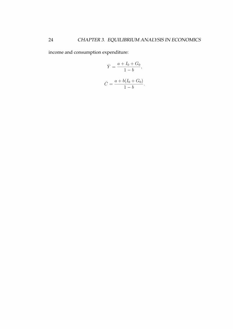
24 CHAPTER 3. EQUILIBRIUM ANALYSIS IN ECONOMICS
income and consumption expenditure:
Y = a+ I0 +G0
1 − b,
C = a+ b(I0 +G0)1 − b
.

Chapter 4
Linear Models and Matrix
Algebra
From the last chapter we have seen that for the one-commodity partial
market equilibrium model, the solutions for P and Q are relatively sim-
ple, even though a number of parameters are involved. As more and
more commodities are incorporated into the model, such solutions for-
mulas quickly become cumbersome and unwieldy. We need to have new
methods suitable for handing a large system of simultaneous equations.
Such a method is provided in matrix algebra.
Matrix algebra can enable us to do many things, including: (1) It pro-
vides a compact way of writing an equation system, even an extremely
large one. (2) It leads to a way of testing the existence of a solution with-
out actually solving it by evaluation of a determinant – a concept closely
related to that of a matrix. (3) It gives a method of finding that solution if
it exists.
Throughout the lecture notes, we will use a bold letter such as a to
denote a vector or a bold capital letter such as A to denote a matrix.
25

26 CHAPTER 4. LINEAR MODELS AND MATRIX ALGEBRA
4.1 Matrix and Vectors
In general, a system of m linear equations in n variables (x1, x2, · · · , xn)can be arranged into such formula
a11x1 + a12x2 + · · · a1nxn = d1,
a21x1 + a22x2 + · · · a2nxn = d2,
· · ·am1x1 + am2x2 + · · · amnxn = dm,
(4.1.1)
where the double-subscripted symbol aij represents the coefficient appear-
ing in the ith equation and attached to the jth variable xj , and dj represents
the constant term in the jth equation.
Example 4.1.1 The two-commodity linear market model can be written –
after eliminating the quantity variables – as a system of two linear equa-
tions.
c1P1 + c2P2 = −c0,
γ1P1 + γ2P2 = −γ0.
Matrix as Arrays
There are essentially three types of ingredients in the equation system
(3.1). The first is the set of coefficients aij ; the second is the set of vari-
ables x1, x2, · · · , xn; and the last is the set of constant terms d1, d2, · · · , dm.
If we arrange the three sets as three rectangular arrays and label them,
respectively, by bold A, x, and d, then we have
A =
a11 a12 · · · a1n
a21 a22 · · · a2n
· · · · · · · · · · · ·am1 am2 · · · amn
,

4.1. MATRIX AND VECTORS 27
x =
x1
x2
· · ·xn
, (3.2)
d =
d1
d2
· · ·dm
.
Example 4.1.2 Given the linear-equation system:
6x1 + 3x2 + x3 = 22x1 + 4x2 − 2x3 = 124x1 − x2 + 5x3 = 10
,
we can write
A =
6 3 11 4 −24 −1 5
,
x =
x1
x2
x3
,
d =
221210
.
Each of these three arrays given above constitutes a matrix.
A matrix is defined as a rectangular array of numbers, parameters, or
variables. As a shorthand device, the array in matrix A can be written

28 CHAPTER 4. LINEAR MODELS AND MATRIX ALGEBRA
more simple as
A = [aij]m×n (i = 1, 2, · · · ,m; j = 1, 2, · · · , n).
Vectors as Special Matrices
The number of rows and number of columns in a matrix together define
the dimension of the matrix. For instance, A is said to be of dimension
m × n. In the special case where m = n, the matrix is called a square
matrix.
If a matrix contains only one column (row), it is called a column (row)
vector. For notation purposes, a row vector is often distinguished from a
column vector by the use of a primed symbol.
x′ = [x1, x2, · · · , xn].
Remark 4.1.1 A vector is merely an ordered n-tuple and as such it may be
interpreted as a point in an n-dimensional space.
With the matrices defined in (3.2), we can express the equations system
(3.1) simply as
Ax = d.
However, the equation Ax = d prompts at least two questions. How
do we multiply two matrices A and x? What is meant by the equality of
Ax and d? Since matrices involve whole blocks of numbers, the familiar
algebraic operations defined for single numbers are not directly applica-
ble, and there is need for new set of operation rules.

4.2. MATRIX OPERATIONS 29
4.2 Matrix Operations
The Equality of Two Matrices
A = B if and only if aij = bij for all i = 1, 2, · · · ,m, j = 1, 2, · · · , n.
Addition and Subtraction of Matrices
A + B = [aij] + [bij] = [aij + bij],
i.e., the addition of A and B is defined as the addition of each pair of
corresponding elements.
Remark 4.2.1 Two matrices can be added (equal) if and only if they have
the same dimension.
Example 4.2.1 4 92 1
+
2 00 7
=
6 92 8
.Example 4.2.2
a11 a12 a13
a21 a22 a23
+
b11 b12 b13
b21 b22 b23
=
a11 + b11 a12 + b12 a13 + b13
a21 + b21 a22 + b22 a23 + b23
.
The Subtraction of Matrices:
A − B is defined by
[aij] − [bij] = [aij − bij].
Example 4.2.3 19 32 0
−
6 81 3
=
13 −51 −3
.

30 CHAPTER 4. LINEAR MODELS AND MATRIX ALGEBRA
Scalar Multiplication:
λA = λ[aij] = [λaij],
i.e., to multiply a matrix by a number is to multiply every element of that
matrix by the given scalar.
Example 4.2.4
7
3 −10 5
=
21 −70 35
.Example 4.2.5
−1
a11 a12 a13
a21 a22 a23
=
−a11 −a12 −a13
−a21 −a22 −a23
.
Multiplication of Matrices:
Given two matrices Am×n and Bp×q, the conformability condition for mul-
tiplication AB is that the column dimension of A must be equal to the row
dimension of B, i.e., the matrix product AB will be defined if and only if
n = p. If defined, the product AB will have the dimension m× q.
The product AB is defined by
AB = C
with cij = ai1b1j + ai2b2j + · · · + ainbnj = ∑nl=1 ailblj.
Example 4.2.6
a11 a12
a21 a22
b11 b12
b21 b22
=
a11b11 + a12b21 a11b12 + a12b22
a21b11 + a22b21 a21b12 + a22b22
.

4.2. MATRIX OPERATIONS 31
Example 4.2.7
3 54 6
−1 0
4 7
=
−3 + 20 35−4 + 24 42
=
17 3520 42
.
Example 4.2.8
u′ = [u1, u2, · · · , un] and v′ = [v1, v2, · · · , vn],
u′v = u1v1 + u2v2 + · · · + unvn =n∑i=1
uivi.
This can be described by using the concept of the inner product of two
vectors u and v.
v · v = u1v1 + u2v2 + · · · + unvn = u′v.
Example 4.2.9 For the linear-equation system (4.1.1), the coefficient matrix
and the variable vector are:
A =
a11 a12 · · · a1n
a21 a22 · · · a2n
· · · · · · · · · · · ·am1 am2 · · · amn
and x =
x1
x2
· · ·xn
,
and we then have
Ax =
a11x1 + a12x2 + · · · + a1nxn
a21x1 + a22x2 + · · · + a2nxn
· · ·am1x1 + am2x2 + · · · + amnxn
.

32 CHAPTER 4. LINEAR MODELS AND MATRIX ALGEBRA
Thus, the linear-equation system (4.1.1) can indeed be simply written as
Ax = d.
Example 4.2.10 Given u =
32
and v′ = [1, 4, 5], we have
uv′ =
3 × 1 3 × 4 3 × 52 × 1 2 × 4 2 × 5
=
3 12 152 8 10
.It is important to distinguish the meaning of uv′ (a matrix with dimension
n× n) and u′v (a 1 × 1 matrix, or a scalar).
4.3 Linear Dependance of Vectors
Definition 4.3.1 A set of vectors v1, · · · ,vn is said to be linearly depen-
dent if and only if one of them can be expressed as a linear combination of
the remaining vectors; otherwise they are linearly independent.
Example 4.3.1 The three vectors
v1 =
27
, v2 =
18
, v3 =
45
are linearly dependent since v3 is a linear combination of v1 and v2;
3v1 − 2v2 =
621
−
216
=
45
= v3
or
3v1 − 2v2 − v3 = 0,
4.4. COMMUTATIVE, ASSOCIATIVE, AND DISTRIBUTIVE LAWS 33
where 0 =
00
represents a zero vector.
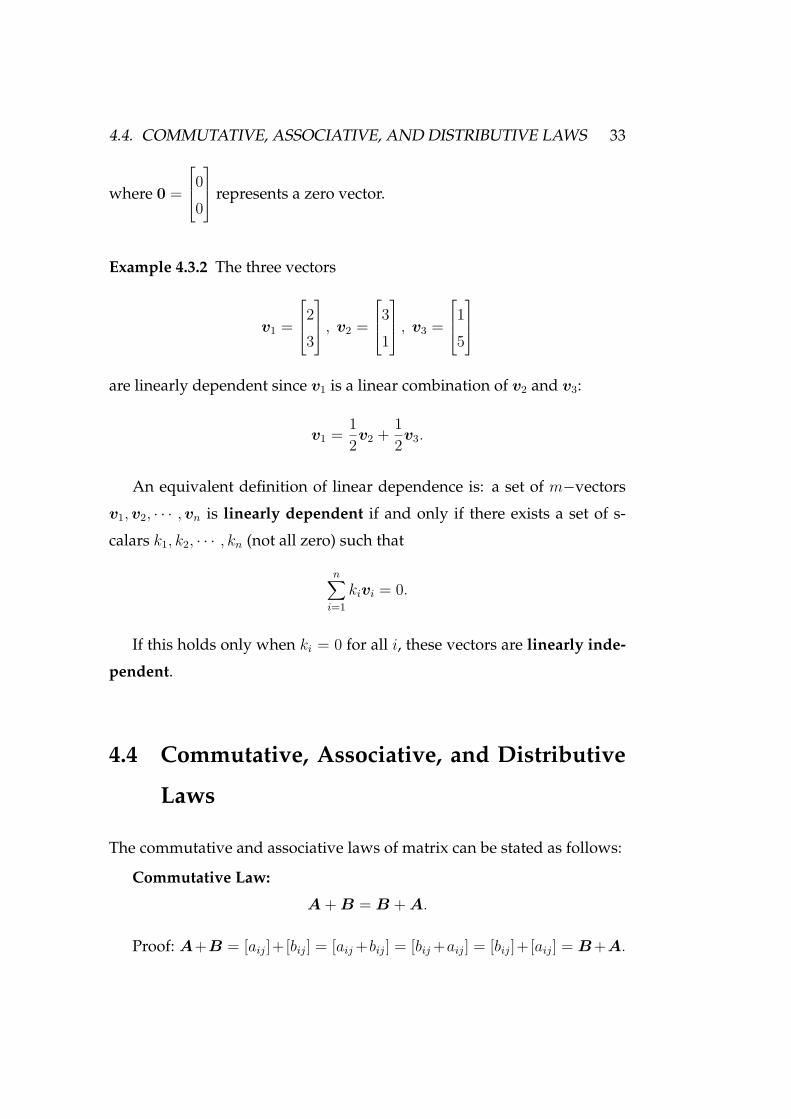
Example 4.3.2 The three vectors
v1 =
23
, v2 =
31
, v3 =
15
are linearly dependent since v1 is a linear combination of v2 and v3:
v1 = 12
v2 + 12
v3.
An equivalent definition of linear dependence is: a set of m−vectors
v1,v2, · · · ,vn is linearly dependent if and only if there exists a set of s-
calars k1, k2, · · · , kn (not all zero) such that
n∑i=1
kivi = 0.
If this holds only when ki = 0 for all i, these vectors are linearly inde-
pendent.
4.4 Commutative, Associative, and Distributive
Laws
The commutative and associative laws of matrix can be stated as follows:
Commutative Law:
A + B = B + A.
Proof: A+B = [aij]+[bij] = [aij+bij] = [bij+aij] = [bij]+[aij] = B +A.

34 CHAPTER 4. LINEAR MODELS AND MATRIX ALGEBRA
Associative Law:
(A + B) + C = A + (B + C).
Proof: (A + B) + C = ([aij] + [bij]) + [cij] = [aij + bij] + [cij] = [aij + bij +cij] = [aij+(bij+cij)] = [aij]+([bij+cij]) = [aij]+([bij]+[cij]) = A+(B+C).
Matrix Multiplication
Matrix multiplication is not commutative, that is,
AB = BA.
Even when AB is defined, BA may not be; but even if both products
are defined, AB = BA may not hold.
Example 4.4.1 Let A =
1 23 4
, B =
0 −16 7
. Then AB =
12 1324 25
, but
BA =
−3 −427 40
.
The scalar multiplication of a matrix does obey. The commutative law:
kA = Ak
if k is a scalar.
Associative Law:
(AB)C = A(BC)
provided A is m× n, B is n× p, and C is p× q.
Distributive Law
A(B + C) = AB + AC [premultiplication by A];

4.5. IDENTITY MATRICES AND NULL MATRICES 35
(B + C)A = BA + CA [postmultiplication by A].
4.5 Identity Matrices and Null Matrices
Definition 4.5.1 Identity matrix is a square matrix with ones in its princi-
pal diagonal and zeros everywhere else.
It is denoted by I or In in which n indicates its dimension.
Fact 1: Given an m× n matrix A, we have
ImA = AIn = A.
Fact 2:
Am×nInBn×p = (AI)B = AB.
Fact 3:
(In)k = In.
Idempotent Matrices: A matrix A is said to be idempotent if AA = A.
Null Matrices: A null–or zero matrix–denoted by 0, plays the role of
the number 0. A null matrix is simply a matrix whose elements are all
zero. Unlike I , the zero matrix is not restricted to being square. Null
matrices obey the following rules of operation.
Am×n + 0m×n = Am×n;
Am×n0n×p = 0m×p;
0q×mAm×n = 0q×n.

36 CHAPTER 4. LINEAR MODELS AND MATRIX ALGEBRA
Remark 4.5.1 (a) CD = CE does not imply D = E. For instance, for
C =
2 36 9
, D =
1 11 2
, E =
−2 13 2
,we have
CD = CE =
5 815 24
,even though D = E.
Then a question is: Under what condition, does CD = CE imply
D = E? We will show that it is so if C has the inverse that we will discuss
shortly.
(b) Even if A and B = 0, we can still have AB = 0. Again, we will see
this is not true if A or B has the inverse.
Example 4.5.1 A =
2 41 2
, B =
−2 41 −2
.
We have AB = 0.
4.6 Transposes and Inverses
The transpose of a matrix A is a matrix which is obtained by interchanging
the rows and columns of the matrix A. Formally, we have
Definition 4.6.1 A matrix B = [bij]n×m is said to be the transpose of A =[aij]m×n if aji = bij for all i = 1, · · · , n and j = 1, · · · ,m.
Usually transpose is denoted by A′ or AT .
Recipe - How to Find the Transpose of a Matrix:
The transpose A′ of A is obtained by making the columns of A into the
rows of A′.

4.6. TRANSPOSES AND INVERSES 37
Example 4.6.1 For A =
3 8 −91 0 4
, its transpose is
A′ =
3 18 0
−9 4
.
Thus, by definition, if the dimension of a matrix A is m × n, then the
dimension of its transpose A′ must be n×m.
Example 4.6.2 For
D =
1 0 40 3 74 7 2
,its transpose is:
D′ =
1 0 40 3 74 7 2
= D.
Definition 4.6.2 A matrix A is said to be symmetric if A′ = A.
A matrix A is called anti-symmetric (or skew-symmetric) if A′ = −A.
A matrix A is called orthogonal if A′A = I .
Properties of Transposes:
a) (A′)′ = A;
b) (A + B)′ = A′ + B′;
c) (αA)′ = αA′ where α is a real number;
d) (AB)′ = B′A′.
The property d) states that the transpose of a product is the product of the
transposes in reverse order.

38 CHAPTER 4. LINEAR MODELS AND MATRIX ALGEBRA
Inverses and Their Properties
For a given square matrix A, while its transpose A′ is always derivable, its
inverse matrix may or may not exist.
Definition 4.6.3 A matrix, denoted by A−1, is the inverse of A if the fol-
lowing conditions are satisfied:
(1) A is a square matrix;
(2) AA−1 = A−1A = I.
Remark 4.6.1 The following statements are true:
1. Not every square matrix has an inverse. Squareness is a nec-
essary but not sufficient condition for the existence of an
inverse. If a square matrix A has an inverse, A is said to
be nonsingular. If A possesses no inverse, it is said to be a
singular matrix.
2. If A is nonsingular, then A and A−1 are inverse of each other,
i.e., (A−1)−1 = A.
3. If A is n× n, then A−1 is also n× n.
4. The inverse of A is unique.
Proof. Let B and C both be inverses of A. Then
B = BI = BAC = IC = C.
5. AA−1 = I implies A−1A = I .
Proof. We need to show that if AA−1 = I , and if there is a
matrix B such that BA = I , then B = A−1. To see this,
postmultiplying both sides of BA = I by A−1, we have
BAA−1 = A−1 and thus B = A−1.

4.6. TRANSPOSES AND INVERSES 39
Example 4.6.3 Let A =
3 10 2
and B = 16
2 −10 3
. Then
AB =
3 10 2
2 −10 3
16
=
66
16
=
11
.So B is the inverse of A.
6. Suppose A and B are nonsingular matrices with dimension n× n.
(a) (AB)−1 = B−1A−1;(b) (A′)−1 = (A−1)′.
Inverse Matrix and Solution of Linear-Equation System
The application of the concept of inverse matrix to the solution of a simul-
taneous linear-equation system is immediate and direct. Consider
Ax = d.
If A is a nonsingular matrix, then premultiplying both sides of Ax = d,
we have
A−1Ax = A−1d.
So, x = A−1d is the solution of Ax = d and the solution is unique since
A−1 is unique. Methods of testing the existence of the inverse and of its
calculation will be discussed in the next chapter.

40 CHAPTER 4. LINEAR MODELS AND MATRIX ALGEBRA

Chapter 5
Linear Models and Matrix
Algebra (Continued)
In chapter 4, it was shown that a linear-equation system can be written
in a compact notation. Moreover, such an equation system can be solved
by finding the inverse of the coefficient matrix, provided the inverse ex-
ists. This chapter studies how to test for the existence of the inverse and
how to find that inverse, and consequently give the ways of solving linear
equation systems.
5.1 Conditions for Nonsingularity of a Matrix
As was pointed out earlier, the squareness condition is necessary but not
sufficient for the existence of the inverse A−1 of a matrix A.
Conditions for Nonsingularity
When the squareness condition is already met, a sufficient condition
for the nonsingularity of a matrix is that its rows (or equivalently, its column-
s) are linearly independent. In fact, the necessary and sufficient conditions
41

42CHAPTER 5. LINEAR MODELS AND MATRIX ALGEBRA (CONTINUED)
for nonsingularity are that the matrix satisfies the squareness and linear
independence conditions.
An n × n coefficient matrix A can be considered an ordered set of row
vectors:
A =
a11 a12 · · · a1n
a21 a22 · · · a2n
· · · · · · · · ·an1 an2 · · · ann
=
v′1
v′2
· · ·v′n
where v′
i = [ai1, ai2, · · · , ain], i = 1, 2, · · · , n. For the rows to be linearly
independent, for any set of scalars ki,∑ni=1 kivi = 0 if and only if ki = 0 for
all i, which is equivalently to say that the linear-equation system
Ak = 0
has the unique solution k = 0, where its transpose k′ = (k1, k2, . . . , kn).This is true when A is nonsingular, i.e., has the inverse.
Example 5.1.1 For a given matrix,
3 4 50 1 26 8 10
,
since v′3 = 2v′
1 + 0v′2, so the matrix is singular.
Example 5.1.2 B =
1 23 4
is nonsingular since their two rows are not
proportional.
Example 5.1.3 C =
−2 16 −3
is singular their two rows are proportional.

5.2. TEST OF NONSINGULARITY BY USE OF DETERMINANT 43
Rank of a Matrix
The above discussion on row independence are regard to square ma-
trices, it is equally applicable to any m× n rectangular matrix.
Definition 5.1.1 A matrix Am×n is said to be of rank γ if the maximum
number of linearly independent rows that can be found in such a matrix
is γ.
The rank also tells us the maximum number of linearly independent
columns in the matrix. Then rank of an m × n matrix can be at most m or
n, whichever is smaller.
By definition, an n×n nonsingular matrix A has n linearly independent
rows (or columns); consequently it must be of rank n. Conversely, an n×n
matrix having rank n must be nonsingular.
5.2 Test of Nonsingularity by Use of Determi-
nant
To determine whether a square matrix is nonsingular by finding the in-
verse of the matrix is not an easy job. However, we can use the determi-
nant of the matrix to easily determine if a square matrix is nonsingular.
Determinant and Nonsingularity
The determinant of a square matrix A, denoted by |A|, is a uniquely
defined scalar associated with that matrix. Determinants are defined only
for square matrices. For a 2 × 2 matrix:
A =
a11 a12
a21 a22
,

44CHAPTER 5. LINEAR MODELS AND MATRIX ALGEBRA (CONTINUED)
its determinant is defined as follows:
|A| =
∣∣∣∣∣∣∣a11 a12
a21 a22
∣∣∣∣∣∣∣ = a11a22 − a12a21.
In view of the dimension of matrix A, |A| as defined in the above is
called a second-order determinant.
Example 5.2.1 Given A =
10 48 5
and B =
3 50 −1
, then
|A| =
∣∣∣∣∣∣∣10 48 5
∣∣∣∣∣∣∣ = 50 − 32 = 18;
|B| =
∣∣∣∣∣∣∣3 50 −1
∣∣∣∣∣∣∣ = −3 − 5 × 0 = −3.
Example 5.2.2 A =
2 68 24
. Then its determinant is
|A| =
∣∣∣∣∣∣∣2 68 24
∣∣∣∣∣∣∣ = 2 × 24 − 6 × 8 = 48 − 48 = 0.
This example shows that the determinant is equal to zero if and only if its
rows are linearly dependent. As will be seen, the value of a determinant |A|can serve as a criterion for testing the linear independence of the rows
(hence nonsingularity) of matrix A but also as an input in the calculation
of the inverse A−1, if it exists.

5.2. TEST OF NONSINGULARITY BY USE OF DETERMINANT 45
Evaluating a Third-Order Determinant
For a 3 × 3 matrix A, its third-order determinants have the value
|A| =
∣∣∣∣∣∣∣∣∣∣a11 a12 a13
a21 a22 a23
a31 a32 a33
∣∣∣∣∣∣∣∣∣∣= a11
∣∣∣∣∣∣∣a22 a23
a32 a33
∣∣∣∣∣∣∣− a12
∣∣∣∣∣∣∣a21 a23
a31 a33
∣∣∣∣∣∣∣+ a13
∣∣∣∣∣∣∣a21 a22
a31 a32
∣∣∣∣∣∣∣= a11a22a33 − a11a23a32 − a12a21a33 + a12a23a31 + a13a21a32 − a13a22a31.
We can use the following diagram to calculate the third-order determi-
nant.
Figure 5.1: The graphic illustration for calculating the third-order determi-nant.
46CHAPTER 5. LINEAR MODELS AND MATRIX ALGEBRA (CONTINUED)
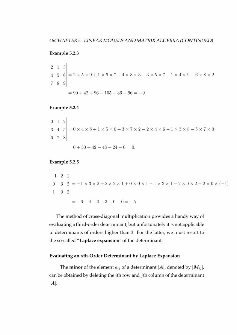
Example 5.2.3
∣∣∣∣∣∣∣∣∣∣2 1 34 5 67 8 9
∣∣∣∣∣∣∣∣∣∣= 2 × 5 × 9 + 1 × 6 × 7 + 4 × 8 × 3 − 3 × 5 × 7 − 1 × 4 × 9 − 6 × 8 × 2
= 90 + 42 + 96 − 105 − 36 − 96 = −9.
Example 5.2.4
∣∣∣∣∣∣∣∣∣∣0 1 23 4 56 7 8
∣∣∣∣∣∣∣∣∣∣= 0 × 4 × 8 + 1 × 5 × 6 + 3 × 7 × 2 − 2 × 4 × 6 − 1 × 3 × 8 − 5 × 7 × 0
= 0 + 30 + 42 − 48 − 24 − 0 = 0.
Example 5.2.5
∣∣∣∣∣∣∣∣∣∣−1 2 10 3 21 0 2
∣∣∣∣∣∣∣∣∣∣= −1 × 3 × 2 + 2 × 2 × 1 + 0 × 0 × 1 − 1 × 3 × 1 − 2 × 0 × 2 − 2 × 0 × (−1)
= −6 + 4 + 0 − 3 − 0 − 0 = −5.
The method of cross-diagonal multiplication provides a handy way of
evaluating a third-order determinant, but unfortunately it is not applicable
to determinants of orders higher than 3. For the latter, we must resort to
the so-called “Laplace expansion" of the determinant.
Evaluating an nth-Order Determinant by Laplace Expansion
The minor of the element aij of a determinant |A|, denoted by |Mij|,can be obtained by deleting the ith row and jth column of the determinant
|A|.

5.2. TEST OF NONSINGULARITY BY USE OF DETERMINANT 47
For instance, for a third determinant, the minors of a11, a12 and a13 are
|M11| =
∣∣∣∣∣∣∣a22 a23
a32 a33
∣∣∣∣∣∣∣ , |M12| =
∣∣∣∣∣∣∣a21 a23
a31 a33
∣∣∣∣∣∣∣ , |M13| =
∣∣∣∣∣∣∣a21 a21
a31 a32
∣∣∣∣∣∣∣ .
A concept closely related to the minor is that of the cofactor. A cofactor,
denoted by Cij , is a minor with a prescribed algebraic sign attached to it.
Formally, it is defined by
|Cij| = (−1)i+j|Mij| =
−|Mij| if i+ j is odd;|Mij| if i+ j is even.
Thus, if the sum of the two subscripts i and j in Mij is even, then
|Cij| = |Mij|. If it is odd, then |Cij| = −|Mij|.
Using these new concepts, we can express a third-order determinant as
|A| = a11|M11| − a12|M12| + a13|M13|
= a11|C11| + a12|C12| + a13|C13|.
The Laplace expansion of a third-order determinant serves to reduce
the evaluation problem to one of evaluating only certain second-order de-
terminants. In general, the Laplace expansion of an nth-order determinant will
reduce the problem to one of evaluating n cofactors, each of which is of the (n−1)thorder, and the repeated application of the process will methodically lead to
lower and lower orders of determinants, eventually culminating in the ba-
sic second-order determinants. Then the value of the original determinant
can be easily calculated.
Formally, the value of a determinant |A| of order n can be found by the

48CHAPTER 5. LINEAR MODELS AND MATRIX ALGEBRA (CONTINUED)
Laplace expansion of any row or any column as follows:
|A| =n∑j=1
aij|Cij| [expansion by the ith row]
=n∑i=1
aij|Cij| [expansion by the jth column].
Even though one can expand |A| by any row or any column, as the
numerical calculation is concerned, a row or column with largest number of
0’s or 1’s is always preferable for this purpose, because a 0 times its cofactor is
simply 0.
Example 5.2.6 For the |A| =
∣∣∣∣∣∣∣∣∣∣5 6 12 3 07 −3 0
∣∣∣∣∣∣∣∣∣∣, the easiest way to expand the
determinant is by the third column, which consists of the elements 1, 0,
and 0. Thus,
|A| = 1 × (−1)1+3
∣∣∣∣∣∣∣2 37 −3
∣∣∣∣∣∣∣ = −6 − 21 = −27.
Example 5.2.7
∣∣∣∣∣∣∣∣∣∣∣∣∣
0 0 0 10 0 2 00 3 0 04 0 0 0
∣∣∣∣∣∣∣∣∣∣∣∣∣= 1 × (−1)1+4
∣∣∣∣∣∣∣∣∣∣0 0 20 3 04 0 0
∣∣∣∣∣∣∣∣∣∣= −1 × (−24) = 24.
A triangular matrix is a special type of square matrix. A square matrix
is called the lower triangular if all the entries above the main diagonal
are zero. Similarly, a square matrix is called the upper triangular if all the
entries below the main diagonal are zero.

5.3. BASIC PROPERTIES OF DETERMINANTS 49
Example 5.2.8 (Upper Triangular Determinant) This example shows that
the value of an upper triangular determinant is the product of all elements
on the main diagonal.
∣∣∣∣∣∣∣∣∣∣∣∣∣
a11 a12 · · · a1n
0 a22 · · · a2n
· · · · · · · · · · · ·0 0 · · · ann
∣∣∣∣∣∣∣∣∣∣∣∣∣= a11 × (−1)1+1
∣∣∣∣∣∣∣∣∣∣∣∣∣
a22 a23 · · · a2n
0 a33 · · · a3n
· · · · · · · · · · · ·0 0 · · · ann
∣∣∣∣∣∣∣∣∣∣∣∣∣
= a11 × a22 × (−1)1+1
∣∣∣∣∣∣∣∣∣∣∣∣∣
a33 a34 · · · a3n
0 a44 · · · a4n
· · · · · · · · · · · ·0 0 · · · ann
∣∣∣∣∣∣∣∣∣∣∣∣∣= · · · = a11 × a22 × ann.
5.3 Basic Properties of Determinants
Property I. The determinant of a matrix A has the same value as that of its
transpose A′, i.e.,
|A| = |A′|.
Example 5.3.1 For
|A| =
∣∣∣∣∣∣∣a b
c d
∣∣∣∣∣∣∣ = ad− bc,
we have
|A′| =
∣∣∣∣∣∣∣a c
b d
∣∣∣∣∣∣∣ = ad− bc = |A|.
Property II. The interchange of any two rows (or any two columns) will alter
the sign, but not the numerical value of the determinant.

50CHAPTER 5. LINEAR MODELS AND MATRIX ALGEBRA (CONTINUED)
Example 5.3.2
∣∣∣∣∣∣∣a b
c d
∣∣∣∣∣∣∣ = ad− bc, but the interchange of the two rows yields
∣∣∣∣∣∣∣c d
a b
∣∣∣∣∣∣∣ = bc− ad = −(ad− bc).
Property III. The multiplication of any one row (or one column) by a scalar
k will change the value of the determinant k-fold, i.e., for |A|,
∣∣∣∣∣∣∣∣∣∣∣∣∣∣∣∣∣
a11 a12 · · · a1n
· · · · · · · · · · · ·kai1 kai2 · · · kain
· · · · · · · · · · · ·an1 an2 · · · ann
∣∣∣∣∣∣∣∣∣∣∣∣∣∣∣∣∣= k
∣∣∣∣∣∣∣∣∣∣∣∣∣∣∣∣∣
a11 a12 · · · a1n
· · · · · · · · · · · ·ai1 ai2 · · · ain
· · · · · · · · · · · ·an1 an2 · · · ann
∣∣∣∣∣∣∣∣∣∣∣∣∣∣∣∣∣= k|A|.
In contrast, the factoring of a matrix requires the presence of a common
divisor for all its elements, as in
k
a11 a12 · · · a1n
a21 a22 · · · a2n
· · · · · · · · ·an1 an2 · · · ann
=
ka11 ka12 · · · ka1n
ka21 ka22 · · · ka2n
· · · · · · · · ·kan1 kan2 · · · kann
.
Property IV. The addition (subtraction) of a multiple of any row (or column)
to (from) another row (or column) will leave the value of the determinant unal-
tered.
This is an extremely useful property, which can be used to greatly sim-
plify the computation of a determinant.
5.3. BASIC PROPERTIES OF DETERMINANTS 51
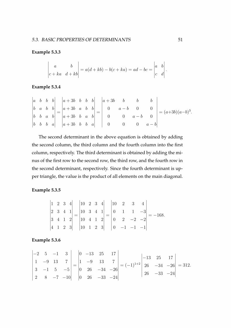
Example 5.3.3
∣∣∣∣∣∣∣a b
c+ ka d+ kb
∣∣∣∣∣∣∣ = a(d+ kb) − b(c+ ka) = ad− bc =
∣∣∣∣∣∣∣a b
c d
∣∣∣∣∣∣∣ .Example 5.3.4
∣∣∣∣∣∣∣∣∣∣∣∣∣
a b b b
b a b b
b b a b
b b b a
∣∣∣∣∣∣∣∣∣∣∣∣∣=
∣∣∣∣∣∣∣∣∣∣∣∣∣
a+ 3b b b b
a+ 3b a b b
a+ 3b b a b
a+ 3b b b a
∣∣∣∣∣∣∣∣∣∣∣∣∣=
∣∣∣∣∣∣∣∣∣∣∣∣∣
a+ 3b b b b
0 a− b 0 00 0 a− b 00 0 0 a− b
∣∣∣∣∣∣∣∣∣∣∣∣∣= (a+3b)(a−b)3.
The second determinant in the above equation is obtained by adding
the second column, the third column and the fourth column into the first
column, respectively. The third determinant is obtained by adding the mi-
nus of the first row to the second row, the third row, and the fourth row in
the second determinant, respectively. Since the fourth determinant is up-
per triangle, the value is the product of all elements on the main diagonal.
Example 5.3.5
∣∣∣∣∣∣∣∣∣∣∣∣∣
1 2 3 42 3 4 13 4 1 24 1 2 3
∣∣∣∣∣∣∣∣∣∣∣∣∣=
∣∣∣∣∣∣∣∣∣∣∣∣∣
10 2 3 410 3 4 110 4 1 210 1 2 3
∣∣∣∣∣∣∣∣∣∣∣∣∣=
∣∣∣∣∣∣∣∣∣∣∣∣∣
10 2 3 40 1 1 −30 2 −2 −20 −1 −1 −1
∣∣∣∣∣∣∣∣∣∣∣∣∣= −168.
Example 5.3.6
∣∣∣∣∣∣∣∣∣∣∣∣∣
−2 5 −1 31 −9 13 73 −1 5 −52 8 −7 −10
∣∣∣∣∣∣∣∣∣∣∣∣∣=
∣∣∣∣∣∣∣∣∣∣∣∣∣
0 −13 25 171 −9 13 70 26 −34 −260 26 −33 −24
∣∣∣∣∣∣∣∣∣∣∣∣∣= (−1)1+2
∣∣∣∣∣∣∣∣∣∣−13 25 1726 −34 −2626 −33 −24
∣∣∣∣∣∣∣∣∣∣= 312.

52CHAPTER 5. LINEAR MODELS AND MATRIX ALGEBRA (CONTINUED)
The second determinant in the above equation is obtained by adding a
multiple 2 of the second row to the first row; a multiple -3 of the second
row to the third row, and a multiple -2 of the second row to the fourth row,
respectively.
Property V. If one row (or column) is a multiple of another row (or column),
the value of the determinant will be zero.
Example 5.3.7 ∣∣∣∣∣∣∣ka kb
a b
∣∣∣∣∣∣∣ = kab− kab = 0.
Remark 5.3.1 Property V is a logic consequence of Property IV.
Property VI. If A and B are both square matrices, then |AB| = |A||B|.
The above basic properties are useful in several ways. For one thing,
they can be of great help in simplifying the task of evaluating determi-
nants. By subtracting multipliers of one row (or column) from another, for
instance, the elements of the determinant may be reduced to much simpler
numbers. If we can indeed apply these properties to transform some row
or column into a form containing mostly 0’s or 1’s, Laplace expansion of
the determinant will become a much more manageable task.
Recipe - How to Calculate the Determinant:
1. The multiplication of any one row (or column) by a scalar k
will change the value of the determinant k-fold.
2. The interchange of any two rows (columns) will change the
sign but not the numerical value of the determinant.
3. If a multiple of any row is added to (or subtracted from)
any other row it will not change the value or the sign of
the determinant. The same holds true for columns (i.e. the

5.3. BASIC PROPERTIES OF DETERMINANTS 53
determinant is not affected by linear operations with rows
(or columns)).
4. If two rows (or columns) are proportional, i.e., they are lin-
early dependent, then the determinant will vanish.
5. The determinant of a triangular matrix is a product of its
principal diagonal elements.
Using these rules, we can simplify the matrix (e.g. obtain as many zero
elements as possible) and then apply Laplace expansion.
Determinantal Criterion for Nonsingularity
Our present concern is primarily to link the linear dependence of
rows with the vanishing of a determinant. By property I, we can easily see
that row independence is equivalent to column independence.
Given a linear-equation system Ax = d, where A is an n×n coefficient
matrix, we have
|A| = 0 ⇔ A is row (or column) independent
⇔ rank(A) = n
⇔ A is nonsingular
⇔ A−1 exists
⇔ a unique solution x = A−1d exists.
Thus the value of the determinant of A provides a convenient criterion
for testing the nonsingularity of matrix A and the existence of a unique
solution to the equation system Ax = d.

54CHAPTER 5. LINEAR MODELS AND MATRIX ALGEBRA (CONTINUED)
Rank of a Matrix Redefined
The rank of a matrix A was earlier defined to be the maximum number
of linearly independent rows in A. In view of the link between row inde-
pendence and the nonvanishing of the determinant, we can redefine the rank
of an m × n matrix as the maximum order of a nonvanishing determinant that
can be constructed from the rows and columns of that matrix. The rank of any
matrix is a unique number.
Obviously, the rank can at most be m or n for a m × n matrix A,
whichever is smaller, because a determinant is defined only for a square
matrix. Symbolically, this fact can be expressed as follows:
γ(A) ≤ min{m,n}.
Example 5.3.8 rank
1 3 22 6 4
−5 7 1
= 2 since
∣∣∣∣∣∣∣∣∣∣1 3 22 6 4
−5 7 1
∣∣∣∣∣∣∣∣∣∣= 0 and
∣∣∣∣∣∣∣1 32 6
∣∣∣∣∣∣∣ = 0.
One can also see this because the first two rows are linearly dependent,
but the last two are independent, therefore the maximum number of lin-
early independent rows is equal to 2.
Properties of the rank:
1) The column rank and the row rank of a matrix are equal.
2) rank(AB) ≤ min{rank(A); rank(B)}.
3) rank(A) = rank(AA′) = rank(A′A).
5.4 Finding the Inverse Matrix
If the matrix A in the linear-equation system Ax = d is nonsingular, then
A−1 exists, and the unique solution of the system will be x = A−1d. We

5.4. FINDING THE INVERSE MATRIX 55
have learned to test the nonsingularity of A by the criterion |A| = 0. The
next question is how we can find the inverse A−1 if A does pass that test.
Expansion of a Determinant by Alien Cofactors
We have known that the value of a determinant |A| of order n can be
found by the Laplace expansion of any row or any column as follows;
|A| =n∑j=1
aij|Cij| [expansion by the ith row]
=n∑i=1
aij|Cij| [expansion by the jth column]
Now what happens if we replace one row (or column) by another row
(or column), i.e., aij by ai′j for i = i′ or by aij′ for j = j′. Then we have the
following important property of determinants.
Property VI. The expansion of a determinant by alien cofactors (the cofac-
tors of a “wrong" row or column) always yields a value of zero. That is, we
have
n∑j=1
ai′j |Cij | = 0 (i = i′) [expansion by the i′th row and use of cofactors of ith row]
n∑j=1
aij′ |Cij | = 0 (j = j′) [expansion by the j′th column and use of cofactors of jth column]
The reason for this outcome lies in the fact that the above formula can
be considered as the result of the regular expansion of a matrix that has
two identical rows or columns.

56CHAPTER 5. LINEAR MODELS AND MATRIX ALGEBRA (CONTINUED)
Example 5.4.1 For the determinant
|A| =
∣∣∣∣∣∣∣∣∣∣a11 a12 a13
a21 a22 a23
a31 a32 a33
∣∣∣∣∣∣∣∣∣∣,
consider another determinant
|A∗| =
∣∣∣∣∣∣∣∣∣∣a11 a12 a13
a11 a12 a13
a31 a32 a33
∣∣∣∣∣∣∣∣∣∣.
If we expand |A∗| by the second row, then we have
0 = |A∗| = a11|C21| + a12|C22| + a13|C23| =3∑j=1
a1j|C2j|.
Matrix Inversion
Property VI provides a way of finding the inverse of a matrix. For a n× n
matrix A:
A =
a11 a12 · · · a1n
a21 a22 · · · a2n
· · · · · · · · ·an1 an2 · · · ann
,
since each element of A has a cofactor |Cij|, we can form a matrix of cofac-
tors by replacing each element aij with its cofactor |Cij|. Such a cofactor
matrix C = [|Cij|] is also n × n. For our present purpose, however, the
transpose of C is of more interest. This transpose C ′ is commonly referred

5.4. FINDING THE INVERSE MATRIX 57
to as the adjoint of A and is denoted by adj A. That is,
C ′ ≡ adj A ≡
|C11| |C21| · · · |Cn1||C12| |C22| · · · |Cn2|· · · · · · · · · · · ·
|C1n| |C2n| · · · |Cnn|
.
By utilizing the formula for the Laplace expansion and Property VI, we
have
AC ′ =
a11 a12 · · · a1n
a21 a22 · · · a2n
· · · · · · · · ·an1 an2 · · · ann
|C11| |C21| · · · |Cn1||C12| |C22| · · · |Cn2|· · · · · · · · · · · ·
|C1n| |C2n| · · · |Cnn|
=
∑nj=1 a1j|C1j|
∑nj=1 a1j|C2j| · · · ∑n
j=1 a1j|Cnj|∑nj=1 a2j|C1j|
∑nj=1 a2j|C2j| · · · ∑n
j=1 a2j|Cnj|· · · · · · · · · · · ·∑n
j=1 anj|C1j|∑nj=1 anj|C2j| · · · ∑n
j=1 anj|Cnj|
=
|A| 0 · · · 00 |A| · · · 0
· · · · · · · · · · · ·0 0 · · · |A|
= |A|In.
Therefore, by the uniqueness of A−1 of A, we know
A−1 = C ′
|A|= adj A
|A|.
Now we have found a way to invert the matrix A.
Remark 5.4.1 In summary, the general procedures for finding the inverse
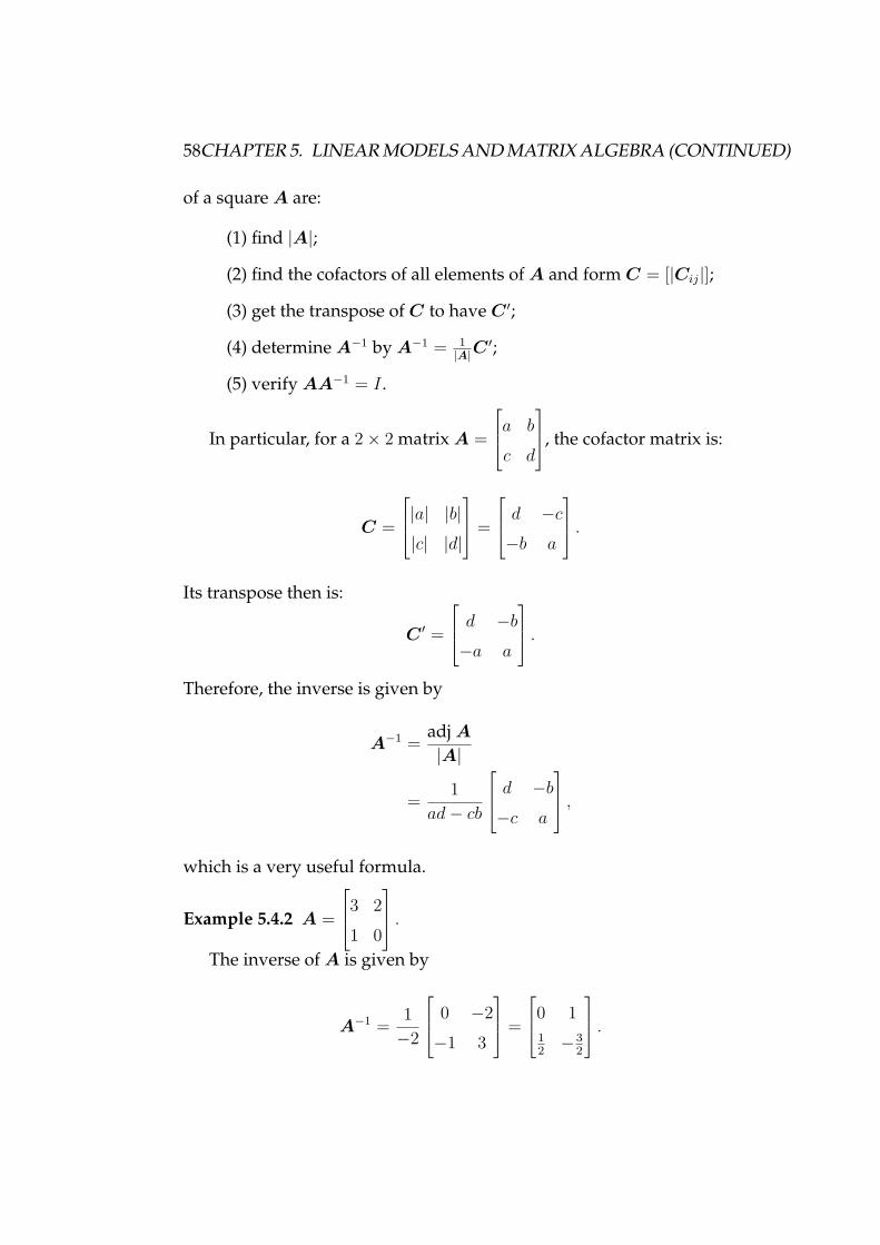
58CHAPTER 5. LINEAR MODELS AND MATRIX ALGEBRA (CONTINUED)
of a square A are:
(1) find |A|;
(2) find the cofactors of all elements of A and form C = [|Cij|];
(3) get the transpose of C to have C ′;
(4) determine A−1 by A−1 = 1|A|C
′;
(5) verify AA−1 = I .
In particular, for a 2 × 2 matrix A =
a b
c d
, the cofactor matrix is:
C =
|a| |b||c| |d|
=
d −c−b a
.Its transpose then is:
C ′ =
d −b−a a
.Therefore, the inverse is given by
A−1 = adj A
|A|
= 1ad− cb
d −b−c a
,which is a very useful formula.
Example 5.4.2 A =
3 21 0
.The inverse of A is given by
A−1 = 1−2
0 −2−1 3
=
0 112 −3
2
.

5.4. FINDING THE INVERSE MATRIX 59
Example 5.4.3 Find the inverse of B =
4 1 −10 3 23 0 7
.
Since |B| = 99 = 0, B−1 exists. The cofactor matrix is
C =
(−1)1+1
∣∣∣∣∣∣∣3 20 7
∣∣∣∣∣∣∣ (−1)1+2
∣∣∣∣∣∣∣0 23 7
∣∣∣∣∣∣∣ (−1)1+3
∣∣∣∣∣∣∣0 33 0
∣∣∣∣∣∣∣(−1)2+1
∣∣∣∣∣∣∣1 −10 7
∣∣∣∣∣∣∣ (−1)2+2
∣∣∣∣∣∣∣4 −13 7
∣∣∣∣∣∣∣ (−1)2+3
∣∣∣∣∣∣∣4 13 0
∣∣∣∣∣∣∣(−1)3+1
∣∣∣∣∣∣∣1 −13 2
∣∣∣∣∣∣∣ (−1)3+2
∣∣∣∣∣∣∣4 −10 2
∣∣∣∣∣∣∣ (−1)3+3
∣∣∣∣∣∣∣4 10 3
∣∣∣∣∣∣∣
=
∣∣∣∣∣∣∣3 20 7
∣∣∣∣∣∣∣ −
∣∣∣∣∣∣∣0 23 7
∣∣∣∣∣∣∣∣∣∣∣∣∣∣0 33 0
∣∣∣∣∣∣∣−
∣∣∣∣∣∣∣1 −10 7
∣∣∣∣∣∣∣∣∣∣∣∣∣∣4 −13 7
∣∣∣∣∣∣∣ −
∣∣∣∣∣∣∣4 13 0
∣∣∣∣∣∣∣∣∣∣∣∣∣∣1 −13 2
∣∣∣∣∣∣∣ −
∣∣∣∣∣∣∣4 −10 2
∣∣∣∣∣∣∣∣∣∣∣∣∣∣4 10 3
∣∣∣∣∣∣∣
=
21 6 −9−7 31 35 −8 12
.
Then
adj B = C ′ =
21 −7 56 31 −8
−9 3 12
.

60CHAPTER 5. LINEAR MODELS AND MATRIX ALGEBRA (CONTINUED)
Therefore, we have
B−1 = 199
21 −7 56 31 −8
−9 3 12
.
Example 5.4.4 A =
2 4 50 3 01 0 1
.
We have |A| = −9 and
A−1 = −19
3 −4 −150 −3 0
−3 4 6
.
5.5 Cramer’s Rule
The method of matrix inversion just discussed enables us to derive a con-
venient way of solving a linear-equation system, known as the Cramer’s
rule.
Derivation of the Cramer’s Rule
Given a linear-equation system Ax = d, the solution can be written as
x = A−1d = 1|A|
(adj A)d

5.5. CRAMER’S RULE 61
provided A is nonsingular. Thus,
x = 1|A|
|C11| |C21| · · · |Cn1||C12| |C22| · · · |Cn2|· · · · · · · · · · · ·
|C1n| |C2n| · · · |Cnn|
d1
d2
· · ·dn
= 1|A|
∑ni=1 di|Ci1|∑ni=1 di|Ci2|
· · ·∑ni=1 di|Cin|
.
That is, the xj is given by
xj = 1|A|
n∑i=1
di|Cij|
= 1|A|
a11 a12 · · · d1 · · · a1n
a21 a22 · · · d2 · · · a2n
· · · · · · · · · · · ·an1 an2 · · · dn · · · ann
= 1
|A||Aj|,
where |Aj| is obtained by replacing the jth column of |A| with constant
terms d1, · · · , dn. This result is the statement of Cramer’s rule.
Example 5.5.1 Let us solve
2 34 −1
x1
x2
=
1210
for x1, x2 using Cramer’s rule. Since
|A| = −14, |A1| = −42, |A2| = −28,
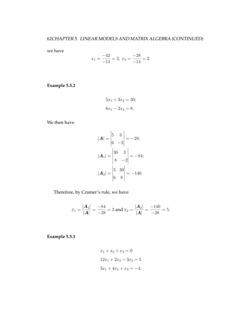
62CHAPTER 5. LINEAR MODELS AND MATRIX ALGEBRA (CONTINUED)
we have
x1 = −42−14
= 3, x2 = −28−14
= 2.
Example 5.5.2
5x1 + 3x2 = 30;
6x1 − 2x2 = 8.
We then have
|A| =
∣∣∣∣∣∣∣5 36 −2
∣∣∣∣∣∣∣ = −28;
|A1| =
∣∣∣∣∣∣∣30 38 −2
∣∣∣∣∣∣∣ = −84;
|A2| =
∣∣∣∣∣∣∣5 306 8
∣∣∣∣∣∣∣ = −140.
Therefore, by Cramer’s rule, we have
x1 = |A1||A|
= −84−28
= 3 and x2 = |A2||A|
= −140−28
= 5.
Example 5.5.3
x1 + x2 + x3 = 0
12x1 + 2x2 − 3x3 = 5
3x1 + 4x2 + x3 = −4.
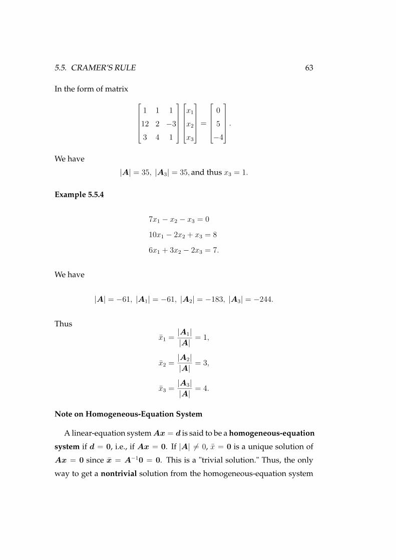
5.5. CRAMER’S RULE 63
In the form of matrix
1 1 112 2 −33 4 1
x1
x2
x3
=
05
−4
.
We have
|A| = 35, |A3| = 35, and thus x3 = 1.
Example 5.5.4
7x1 − x2 − x3 = 0
10x1 − 2x2 + x3 = 8
6x1 + 3x2 − 2x3 = 7.
We have
|A| = −61, |A1| = −61, |A2| = −183, |A3| = −244.
Thus
x1 = |A1||A|
= 1,
x2 = |A2||A|
= 3,
x3 = |A3||A|
= 4.
Note on Homogeneous-Equation System
A linear-equation system Ax = d is said to be a homogeneous-equation
system if d = 0, i.e., if Ax = 0. If |A| = 0, x = 0 is a unique solution of
Ax = 0 since x = A−10 = 0. This is a "trivial solution." Thus, the only
way to get a nontrivial solution from the homogeneous-equation system

64CHAPTER 5. LINEAR MODELS AND MATRIX ALGEBRA (CONTINUED)
is to have |A| = 0, i.e., A is singular. In this case, Cramer’s rule is not
directly applicable. Of course, this does not mean that we cannot obtain
solutions; it means only that the solution is not unique. In fact, it has an
infinite number of solutions.
If r(A) = k < n, we can delete n − k dependent equations from the
homogeneous-equation system Ax = 0, and then apply Cramer’s rule to
any k variables, say (x1, . . . , xk) whose coefficient matrix has a rank k and
constant term in equation i is −(ai,k+1xk+1 + . . . , ainxn).
Example 5.5.5
a11x1 + a12x2 = 0,
a21x2 + a22x2 = 0.
If |A| = 0, then its rows are linearly dependent. As a result, one of two
equations is redundant. By deleting, say, the second equation, we end up
with one equation with two variables. The solutions are
x1 = −a12
a11x2 if a11 = 0
Overview on Solution Outcomes for a linear-Equation System
Proposition 5.5.1 A necessary and sufficient condition for the existence of solu-
tion for a linear-equation system Ax = d is that the rank of A and the rank of
the added matrix [A; d] are the same, i.e.,
r(A) = r([A; d]).
For a linear-equation system Ax = d, our discussion can be summa-
rized as in the following table.

5.6. APPLICATION TO MARKET AND NATIONAL-INCOME MODELS65
|A|d
d = 0 d = 0
|A| = 0 The solution is uniqueand x = 0
The solution is uniqueand x = 0
|A| = 0Equationsdependent
An infinite number ofsolutions and x = 0
There is an infinitenumber of solutions
Equationsinconsistent No solution exists [Not Applicable]
Table 5.1: The summary of solution for linear-equation system Ax = d
5.6 Application to Market and National-Income
Models
Market Model:
The two-commodity model described in chapter 3 can be written as
follows:
c1P1 + c2P2 = −c0,
γ1P1 + γ2P2 = −γ0.
Thus
|A| =
∣∣∣∣∣∣∣c1 c2
γ1 γ2
∣∣∣∣∣∣∣ = c1γ2 − c2γ1,
|A1| =
∣∣∣∣∣∣∣−c0 c2
−γ0 γ2
∣∣∣∣∣∣∣ = c2γ0 − c0γ2,
|A2| =
∣∣∣∣∣∣∣c1 −c0
γ1 −γ0
∣∣∣∣∣∣∣ = c0γ1 − c1γ0.

66CHAPTER 5. LINEAR MODELS AND MATRIX ALGEBRA (CONTINUED)
Thus the equilibrium is given by
P1 = |A1||A|
= c2γ0 − c0γ2
c1γ2 − c2γ1
and
P2 = |A2||A|
= c0γ1 − c1γ0
c1γ2 − c2γ1.
General Market Equilibrium Model:
Consider a market for three goods. The demand and supply for each
good are given by:
D1 = 5 − 2P1 + P2 + P3,
S1 = −4 + 3P1 + 2P2.
D2 = 6 + 2P1 − 3P2 + P3,
S2 = 3 + 2P2.
D3 = 20 + P1 + 2P2 − 4P3,
S3 = 3 + P2 + 3P3,
where Pi is the price of good i; i = 1; 2; 3.
The equilibrium conditions are: Di = Si; i = 1; 2; 3 , that is
5P1 + P2 − P3 = 9,−2P1 + 5P2 − P3 = 3,−P1 − P2 + 7P3 = 17.

5.6. APPLICATION TO MARKET AND NATIONAL-INCOME MODELS67
This system of linear equations can be solved via Cramer’s rule
P1 = |A1||A|
= 356178
= 2,
P2 = |A2||A|
= 356178
= 2,
P3 = |A3||A|
= 534178
= 3.
National-Income Model
Consider the simple national-income model:
Y = C + I0 +G0,
C = a+ bY (a > 0, 0 < b < 1).
These can be rearranged into the form
Y − C = I0 +G0,
−bY + C = a.
While we can solve Y and C by Cramer’s rule, here we solve this model
by inverting the coefficient matrix.
Since A =
1 −1−b 1
, then A−1 = 11−b
1 1b 1
.
Hence
[Y C
]= 1
1 − b
1 1b 1
I0 +G0
a
= 1
1 − b
I0 +G0 + a
b(I0 +G0) + a
.

68CHAPTER 5. LINEAR MODELS AND MATRIX ALGEBRA (CONTINUED)
5.7 Quadratic Forms
Quadratic Forms
Definition 5.7.1 A function q with n-variables is said to have the quadrat-
ic form if it can be written as
q(u1, u2, · · · , un) = d11u21 + 2d12u1u2 + · · · + 2d1nu1un
+ d22u22 + 2d23u2u3 + · · · + 2d2nu2un
· · ·
+ dnnu2n.
If we let dji = dij , i < j, then q(u1, u2, · · · , un) can be written as
q(u1, u2, · · · , un) = d11u21 + d12u1u2 + · · · + d1nu1un
+ d12u2u1 + d22u22 + · · · + d2nu2un
· · ·
+ dn1unu1 + dn2unu2 + · · · + dnnu2n
=n∑i=1
n∑j=1
dijuiuj
= u′Du,
where
D =
d11 d12 · · · d1n
d21 d22 · · · d2n
· · · · · · · · · · · ·dn1 dn2 · · · dnn
,
which is called the quadratic-form matrix.
Since dij = dji, D is a symmetric matrix.

5.7. QUADRATIC FORMS 69
Example 5.7.1 A quadratic form in two variables:
q = d11u21 + d12u1u2 + d22u
22.
The symmetric matrix is d11 d12/2d12/2 d22
.Then we have q = u′Du.
Positive and Negative Definiteness:
Definition 5.7.2 A quadratic form q(u1, u2, · · · , un) = u′Du is said to be
(a) positive definite (PD) if q(u) > 0 for all u = 0;
(b) positive semidefinite (PSD) if q(u) ≥ 0 for all u = 0;
(c) negative definite (ND) if q(u) < 0 for all u = 0;
(d) negative semidefinite (NSD) if q(u) ≤ 0 for all u = 0.
Otherwise q is called indefinite (ID).
Sometimes, we say that a matrix D is, for instance, positive definite if
the corresponding quadratic form q(u) = u′Du is positive definite.
Example 5.7.2
q = u21 + u2
2
is positive definite (PD),
q = (u1 + u2)2
is positive semidefinite (PSD), and
q = u21 − u2
2
is indefinite.
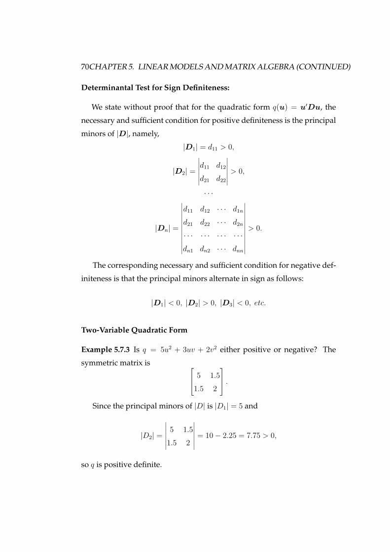
70CHAPTER 5. LINEAR MODELS AND MATRIX ALGEBRA (CONTINUED)
Determinantal Test for Sign Definiteness:
We state without proof that for the quadratic form q(u) = u′Du, the
necessary and sufficient condition for positive definiteness is the principal
minors of |D|, namely,
|D1| = d11 > 0,
|D2| =
∣∣∣∣∣∣∣d11 d12
d21 d22
∣∣∣∣∣∣∣ > 0,
· · ·
|Dn| =
∣∣∣∣∣∣∣∣∣∣∣∣∣
d11 d12 · · · d1n
d21 d22 · · · d2n
· · · · · · · · · · · ·dn1 dn2 · · · dnn
∣∣∣∣∣∣∣∣∣∣∣∣∣> 0.
The corresponding necessary and sufficient condition for negative def-
initeness is that the principal minors alternate in sign as follows:
|D1| < 0, |D2| > 0, |D3| < 0, etc.
Two-Variable Quadratic Form
Example 5.7.3 Is q = 5u2 + 3uv + 2v2 either positive or negative? The
symmetric matrix is 5 1.51.5 2
.Since the principal minors of |D| is |D1| = 5 and
|D2| =
∣∣∣∣∣∣∣5 1.5
1.5 2
∣∣∣∣∣∣∣ = 10 − 2.25 = 7.75 > 0,
so q is positive definite.

5.7. QUADRATIC FORMS 71
Three-Variable Quadratic Form
Example 5.7.4 Determine whether
q = u21 + 6u2
2 + 3u23 − 2u1u2 − 4u2u3
is positive or negative definite. The matrix D corresponding this quadratic
form is
D =
1 −1 0
−1 6 −20 −2 3
,and the principal minors of |D| are
|D1| = 1 > 0,
|D2| =
∣∣∣∣∣∣∣1 −1
−1 6
∣∣∣∣∣∣∣ = 6 − 1 = 5,
and
|D3| =
∣∣∣∣∣∣∣∣∣∣1 −1 0
−1 6 −20 −2 3
∣∣∣∣∣∣∣∣∣∣= 11 > 0.
Thus, the quadratic form is positive definite.
Example 5.7.5 Determine whether
q = −3u21 − 3u2
2 − 5u23 − 2u1u2
is positive or negative definite. The matrix D corresponding this quadratic
form is
D =
−3 −1 0−1 −3 00 0 −5
.
72CHAPTER 5. LINEAR MODELS AND MATRIX ALGEBRA (CONTINUED)
Leading principal minors of D are
|D1| = −3 < 0,
|D2| = 8 > 0,
|D3| = −40 < 0.
Therefore, the quadratic form is negative definite.
5.8 Eigenvalues and Eigenvectors
Consider the matrix equation:
Dx = λx.
Any number λ such that the equation Dx = λx has a non-zero vector-
solution x is called the eigenvalue (or called the characteristic root) of
the above equation. Any non-zero vector x satisfying the above equation
is called the eigenvector (or called the characteristic vector) of D for the
eigenvalue λ.
Recipe - How to calculate eigenvalues:
From Dx = λx, we have the following homogeneous-equation system:
(D − λI)x = 0.
Since we require that x be non-zero, the determinant of (D−λI) should
vanish. Therefore all eigenvalues can be calculated as roots of the equa-
tion (which is often called the characteristic equation or the characteristic
polynomial of D)
|D − λI| = 0.
5.8. EIGENVALUES AND EIGENVECTORS 73
Example 5.8.1 Let
D =
3 −1 0
−1 3 00 0 5
.
|D − λI| =
∣∣∣∣∣∣∣∣∣∣3 − λ −1 0−1 3 − λ 00 0 5 − λ
∣∣∣∣∣∣∣∣∣∣= (5 − λ)(λ− 2)(λ− 4) = 0,
and therefore the eigenvalues are λ1 = 2, λ2 = 4, and λ3 = 5.
Properties of Eigenvalues:
Proposition 5.8.1 A quadratic form q(u1, u2, · · · , un) = u′Du is
positive definite if and only if eigenvalues λi > 0 for all i = 1, 2, · · · , n.
negative definite if and only if eigenvalues λi < 0 for all i = 1, 2, · · · , n.
positive semidefinite if and only if eigenvalues λi ≥ 0 for all i =1, 2, · · · , n.
negative semidefinite if and only if eigenvalues λi ≤ 0 for all i =1, 2, · · · , n
indefinite if at least one positive and one negative eigenvalues exist.
Definition 5.8.1 Matrix A is said to be diagonalizable if there exists a non-
singular matrix P and a diagonal matrix D such that
P −1AP = D.
Matrix U is an orthogonal matrix if U ′ = U−1.

74CHAPTER 5. LINEAR MODELS AND MATRIX ALGEBRA (CONTINUED)
Theorem 5.8.1 (The Spectral Theorem for Symmetric Matrices) Suppose that
A is a symmetric matrix of order n and λ1, · · · , λn are its eigenvalues. Then there
exists an orthogonal matrix U such that
U−1AU =
λ1 0
. . .
0 λn
.
Usually, U is the normalized matrix formed by eigenvectors. It has the
property U ′U = I . "Normalized" means that for any column u of the
matrix U , we have u′u = 1.
Example 5.8.2 Diagonalize the matrix
A =
1 22 4
.
First, we need to find the eigenvalues:
∣∣∣∣∣∣∣1 − λ 2
2 4 − λ
∣∣∣∣∣∣∣ = λ(λ− 5) = 0,
i.e., λ1 = 0 and λ2 = 5.
For λ1 = 0, we solve
1 − 0 22 4 − 0
x1
x2
=
00
.
The eigenvector, corresponding to λ1 = 0, is v1 = C1 · (2,−1)′, where C1
is an arbitrary real constant. Similarly, for λ2 = 5, we have v2 = C2 · (1, 2)′.
Let us normalize the eigenvectors, i.e. let us pick constants Ci such that
5.9. VECTOR SPACES 75
v′ivi = 1. We get
v1 =(
2√5,
−1√5
), v2 =
(1√5,
2√5
).
Thus the diagonalization matrix U is
U =
2√5
1√5
−1√5
2√5 .
You can easily check that
U−1AU =
0 00 5
.The trace of a square matrix of order n is the sum of the n elements on
its principal diagonal, i.e., tr(A) = ∑ni=1 aii.
Properties of the Trace:
1) tr(A) = λ1 + · · · + λn;
2) if A and B are of the same order, tr(A+B) = tr(A)+ tr(B);
3) if a is a scalar, tr(aA) = atr(A);
4) tr(AB) = tr(BA), whenever AB is square;
5) tr(A′) = tr(A);
6) tr(A′A) = ∑ni=1
∑nj=1 a
2ij .
5.9 Vector Spaces
A (real) vector space is a nonempty set V of objects together with an addi-
tive operation + : V × V → V , +(u,v) = u + v and a scalar multiplicative
76CHAPTER 5. LINEAR MODELS AND MATRIX ALGEBRA (CONTINUED)
operation · : R ×V → V , ·(a,u) = au which satisfies the following axioms
for any u,v,w ∈ V and any a, b ∈ R where R is the set of all real numbers:
1. (u + v) + w = u + (v + w);
2. u + v = v + u;
3. 0 + u = u;
4. u + (−u) = 0;
5. a(u + v) = au + av;
6. (a+ b)u = au + bu;
7. a(bu) = (ab)u;
8. 1u = u.
The objects of a vector space V are called the vectors, the operations +and · are called the vector addition and scalar multiplication, respectively.
The element 0 ∈ V is the zero vector and −v is the additive inverse of V .
Example 5.9.1 (The n-Dimensional Vector Space Rn) For Rn, consider u,v ∈Rn, u = (u1, u2, · · · , un)′, v = (v1, v2, · · · , vn)′ and a ∈ R. Define the addi-
tive operation and the scalar multiplication as follows:
u + v = (u1 + v1, · · · , un + vn)′,
au = (au1, · · · , aun)′.
It is not difficult to verify that Rn together with these operations is a vector
space.
Let V be a vector space. An inner product or scalar product in V is
a function s : V × V → R, s(u,v) = u · v which satisfies the following
properties:

5.9. VECTOR SPACES 77
1. u · v = v · u,
2. u · (v + w) = u · v + u · w,
3. a(u · v) = (au) · v = u · (av),
4. u · u ≥ 0 and u · u = 0 iff u = 0.
Example 5.9.2 Let u,v ∈ Rn, u = (u1, u2, · · · , un)′, v = (v1, v2, · · · , vn)′.
Then u · v = u1v1 + · · · + unvn.
Let V be a vector space and v ∈ V . The norm of magnitude is a func-
tion || · || : V → R defined as ||v|| =√
v · v. For any v ∈ V and any a ∈ R,
we have the following properties:
1. ||au|| = |a|||u||;
2. ||u + v|| ≤ ||u|| + ||v||;
3. |u · v| ≤ ||u|| × ||v||.
The nonzero vectors u and v are parallel if there exists a ∈ R such that
u = av.
The vectors u and v are orthogonal or perpendicular if their scalar
product is zero, that is, if u · v = 0.
The angle between vectors u and v is arccos( uv||u||||v||)
A nonempty subset S of a vector space V is a subspace of V if for any
u,v ∈ S and a ∈ Ru + v ∈ S and au ∈ S.
Example 5.9.3 V is a subset of itself. {0} is also a subset of V . These
subspaces are called proper subspaces.
Example 5.9.4 L = {(x, y)|y = mx + n} where m,n ∈ R and m = 0 is a
subspace of R2.

78CHAPTER 5. LINEAR MODELS AND MATRIX ALGEBRA (CONTINUED)
Let u1,u2, · · · ,uk be vectors in a vector space V . The set S of all linear
combinations of these vectors
S = {a1u1 + a2u2 + · · · , akuk|a1, · · · , ak ∈ R}
is called the subspace generated or spanned by the vectors u1,u2, · · · ,uk
and denoted as sp(u1,u2, · · · ,uk). One can prove that S is a subspace of
V .
Example 5.9.5 Let u1 = (2,−1, 1)′, u2 = (3, 4, 0)′. Then the subspace of R3
generated by u1 and u2 is
sp(u1,u2) = {(2a+ 3b,−a+ 4b, a)′|a, b ∈ R}.
As we discussed in Chapter 4, a set of vectors {u1,u2, · · · ,uk} in a vec-
tor space V is linearly dependent if there exists the real numbers a1, a2, · · · , ak,
not all zero, such that a1u1 + a2u2 + · · · + akuk = 0. In other words, the
set of vectors in a vector space is linearly dependent if and only if one
vector can be written as a linear combination of the others. A set of vec-
tors {u1,u2, · · · ,uk} in a vector space V is linearly independent if it is not
linearly dependent.
Properties: Let {u1,u2, · · · ,uk} be n vectors in Rn. The following con-
ditions are equivalent:
i) The vectors are independent.
ii) The matrix having these vectors as columns is nonsingular.
iii) The vectors generate Rn.
A set of vectors {u1,u2, · · · ,uk} in V is a basis for V if it, first,
generates V , and, second, is linearly independent.

5.9. VECTOR SPACES 79
Example 5.9.6 Consider the following vectors in Rn. ei = (0, · · · , 0, 1, 0, · · · , 0)′,
where 1 is in the ith position, i = 1, · · · , n. The set En = {e1, e2, · · · , en}forms a basis for Rn which is called the standard basis.
Let V be a vector space and B = {u1,u2, · · · ,uk} a basis for V . Since
B generates V , for any u ∈ V , there exists the real numbers x1, x2, · · · , xnsuch that u = x1u1 + · · · + xnun. The column vector x = (x1, x2, · · · , xn)′
is called the vector of coordinates of u with respect to B.
Example 5.9.7 Consider the vector space Rn with the standard basis En.
For any u = (u1, · · · , un)′, we can represent u as u = u1e1 + · · · + unen;
therefore, (u1, · · · , un)′ is the vector of coordinates of u with respect to En.
Example 5.9.8 Consider the vector space R2. Let us find the coordinate
vector of (−1, 2)′ with respect to the basis B = (1, 1)′, (2,−3)′ (i.e., find
(−1, 2)′B). We have to solve for a, b such that (−1, 2)′ = a(1, 1)′ + b(2,−3)′.
Solving the system a+ 2b = −1 and a− 3b = 2, we find a = 15 and b = −3
5 .
Thus, (−1, 2)′B = (1
5 ,−35)′.
The dimension of a vector space V dim(V ) is the number of elements
in any basis for V .
Example 5.9.9 The dimension of the vector space Rn with the standard
basis En is n.
Let U and V be two vector spaces. A linear transformation of U into V
is a mapping T : U → V such that for any u,v ∈ U and any a, b ∈ R, we
have
T (au + bv) = aT (u) + bT (v).
Example 5.9.10 Let A be a m× n real matrix. The mapping T : Rn → Rm
defined by T (u) = Au is a linear transformation.
80CHAPTER 5. LINEAR MODELS AND MATRIX ALGEBRA (CONTINUED)
Properties:
Let U and V be two vector spaces, B = (b1, · · · , bn) a basis for U and
C = (c1, · · · , cm) a basis for V .
1. Any linear transformation T can be represented by an m ×n matrix AT whose ith column is the coordinate vector of
T (bi) relative to C.
2. If x = (x1, · · · , xn)′ is the coordinate vector of u ∈ U relative
to B and y = (y1, · · · , ym)′ is the coordinate vector of T (u)relative to C, then T defines the following transformation
of coordinates:
y = ATx for any u ∈ U.
The matrix AT is called the matrix representation of T relative to bases
B and C.
Remark 5.9.1 Any linear transformation is uniquely determined by a trans-
formation of coordinates.
Example 5.9.11 Consider the linear transformation T : R3 → R2, T ((x, y, z)′) =(x − 2y, x + z)′ and bases B = {(1, 1, 1)′, (1, 1, 0)′, (1, 0, 0)′} for R3 and
C = {(1, 1)′, (1, 0)′} for R2. How can we find the matrix representation
of T relative to bases B and C?
We have
T ((1, 1, 1)′) = (−1, 2), T ((1, 1, 0)′) = (−1, 1), T ((1, 0, 0)′) = (1, 1).
The columns of AT are formed by the coordinate vectors of T ((1, 1, 1)′),T ((1, 1, 0)′), T ((1, 0, 0)′) relative to C. Applying the procedure developed

5.9. VECTOR SPACES 81
in Example 5.9.8, we find
AT =
2 1 1−3 −2 0
.Let V be a vector space of dimension n, B and C be two bases for V ,
and I : V → V be the identity transformation ((I(v) = v for all v ∈ V ). The
change-of-basis matrix D relative to B, C is the matrix representation of
I to B, C.
Example 5.9.12 For u ∈ V , let x = (x1, · · · , xn)′ be the coordinate vector of
u relative to B and y = (y1, · · · , yn)′ is the coordinate vector of u relative
to C. If D is the change-of-basis matrix relative to B, C then y = Cx. The
change-of-basis matrix relative to C, B is D−1.
Example 5.9.13 Given the following bases for R2: B = {(1, 1)′, (1, 0)′} and
C = {(0, 1)′, (1, 1)′}, find the change-of-basis matrix D relative to B, C.
The columns of D are the coordinate vectors of (1, 1)′, (1, 0)′ relative to C.
Following Example 5.9.8, we find
D =
0 −11 1
.

82CHAPTER 5. LINEAR MODELS AND MATRIX ALGEBRA (CONTINUED)

Chapter 6
Comparative Statics and the
Concept of Derivative
6.1 The Nature of Comparative Statics
Comparative statics is concerned with the comparison of different equilib-
rium states that are associated with different sets of values of parameters
and exogenous variables. When the value of some parameter or exoge-
nous variable that is associated with an initial equilibrium changes, we
will have a new equilibrium. Then the question posed in the comparative-
static analysis is: How would the new equilibrium compare with the old?
It should be noted that in the comparative-statics analysis we don’t
concern with the process of adjustment of the variables; we merely com-
pare the initial (prechange) equilibrium state with the new (postchange)
equilibrium state. We also preclude the possibility of instability of equilib-
rium for we assume the equilibrium to be attainable.
It should be clear that the problem under consideration is essentially
one of finding a rate of change: the rate of change of the equilibrium value
of an endogenous variable with respect to the change in a particular pa-
83

84CHAPTER 6. COMPARATIVE STATICS AND THE CONCEPT OF DERIVATIVE
rameter or exogenous variable. For this reason, the mathematical concept
of derivative takes on preponderant significance in comparative statics.
6.2 Rate of Change and the Derivative
We want to study the rate of change of any variable y in response to a
change in another variable x, where the two variables are related to each
other by the function
y = f(x).
Applied in the comparative static context, the variable y will represent
the equilibrium value of an endogenous variable, and x will be some pa-
rameter.
The Difference Quotient
We use the symbol ∆ to denote the change from one point, say x0, to
another point, say x1. Thus ∆x = x1 − x0. When x changes from an initial
value x0 to a new value x0 +∆x, the value of the function y = f(x) changes
from f(x0) to f(x0 + ∆x). The change in y per unit of change in x can be
represented by the difference quotient.
∆y∆x
= f(x0 + ∆x) − f(x0)∆x
.
Example 6.2.1 y = f(x) = 3x2 − 4.
Then f(x0) = 3x20 − 4, f(x0 + ∆x) = 3(x0 + ∆x)2 − 4,

6.2. RATE OF CHANGE AND THE DERIVATIVE 85
and thus,
∆y∆x
= f(x0 + ∆x) − f(x0)∆x
= 3(x0 + ∆x)2 − 4 − (3x20 − 4)
∆x
= 6x0∆x+ 3(∆x)2
∆x= 6x0 + 3∆x.
The Derivative
Frequently, we are interested in the rate of change of y when ∆x is
very small. In particular, we want to know the rate of ∆y/∆x when ∆xapproaches to zero. If, as ∆x → 0, the limit of the difference quotient
∆y/∆x exits, that limit is called the derivative of the function y = f(x),and the derivative is denoted by
dy
dx≡ y′ ≡ f ′(x) ≡ lim
∆x→0
∆y∆x
.
Remark 6.2.1 Several points should be noted about the derivative: (1) a
derivative is a function. Whereas the difference quotient is a function of x0
and ∆x, the derivative is a function of x0 only; and (2) since the derivative
is merely a limit of the difference quotient, it must also be of necessity a
measure of some rate of change. Since ∆x → 0, the rate measured by the
derivative is in the nature of an instantaneous rate of change.
Example 6.2.2 Referring to the function y = 3x2 − 4 again. Since
∆y∆x
= 6x+ 3∆x,
we have dydx
= 6x.

86CHAPTER 6. COMPARATIVE STATICS AND THE CONCEPT OF DERIVATIVE
6.3 The Derivative and the Slope of a Curve
Elementary economics tells us that, given a total-cost function C = f(Q),where C is the total cost and Q is the output, the marginal cost MC is
defined as MC = ∆C/∆Q. It is a continuous variable, ∆Q will refer to an
infinitesimal change. It is well known that MC can be measured by the
slope of the total cost curve. But the slope of the total-cost curve is nothing
but the limit of the ratio ∆C/∆Q as ∆Q → 0. The concept of the slope
of a curve is then merely the geometric counterpart of the concept of the
derivative.
Figure 6.1: Graphical illustrations of the slope of the total cost curve andthe marginal cost.
6.4. THE CONCEPT OF LIMIT 87
6.4 The Concept of Limit
In the above, we have defined the derivative of a function y = f(x) as the
limit of ∆y/∆x as ∆x → 0. We now study the concept of limit. For a given
function q = q(v), the concept of limit is concerned with the question:
What value does q approach as v approaches a specific value? That is,
as v → N (the N can be any number, say N = 0, N = +∞,−∞), what
happens to limv→N g(v).
When we say v → N , the variable v can approach the number N either
from values greater than N , or from values less than N . If, as v → N from
the left side (from values less than N ), q approaches a finite number L, we
call L the left-side limit of q. Similarly, we call L the right-side limit of q
if v → N from the right side. The left-side limit and right-side limit of q
are denoted by limv→N− q and limv→N+ q, respectively. The limit of q at N
is said to exit if
limv→N−
q = limv→N+
q,
and is denoted by limv→N q. Note that L must be a finite number. If we
have the situation of limv→N q = ∞ (or −∞), we shall consider q to possess
no limit or an "infinite limit." It is important to realize that the symbol ∞is not a number, and therefore it cannot be subjected to the usual algebraic
operations.
Graphical Illustrations
There are several possible situations regrading the limit of a function,
which are shown in the following diagrams.
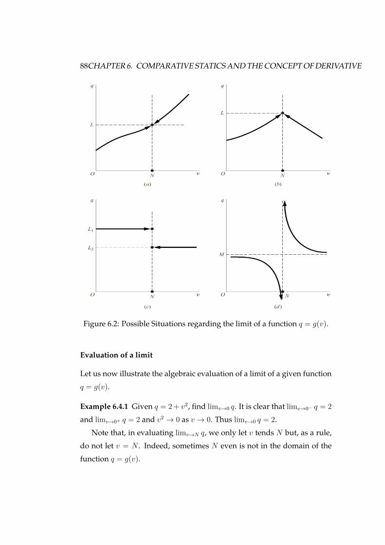
88CHAPTER 6. COMPARATIVE STATICS AND THE CONCEPT OF DERIVATIVE
Figure 6.2: Possible Situations regarding the limit of a function q = g(v).
Evaluation of a limit
Let us now illustrate the algebraic evaluation of a limit of a given function
q = g(v).
Example 6.4.1 Given q = 2 + v2, find limv→0 q. It is clear that limv→0− q = 2and limv→0+ q = 2 and v2 → 0 as v → 0. Thus limv→0 q = 2.
Note that, in evaluating limv→N q, we only let v tends N but, as a rule,
do not let v = N . Indeed, sometimes N even is not in the domain of the
function q = g(v).

6.4. THE CONCEPT OF LIMIT 89
Example 6.4.2 Consider
q = (1 − v2)/(1 − v).
For this function, N = 1 is not in the domain of the function, and we
cannot set v = 1 since it would involve division by zero. Moreover, even
the limit-evaluation procedure of letting v − 1 will cause difficulty since
(1 − v) → 0 as v → 1.
One way out of this difficulty is to try to transform the given ratio to a
form in which v will not appear in the denominator. Since
q = 1 − v2
1 − v= (1 − v)(1 + v)
1 − v= 1 + v (v = 1)
and v → 1 implies v = 1 and (1 + v) → 2 as v → 1, we have limv→1 q = 2.
Example 6.4.3 Find limv→∞2v+5v+1 .
Since 2v+5v+1 = 2(v+1)+3
v+1 = 2 + 3v+1 and limv→∞
3v+1 = 0, so limv→∞
2v+5v+1 = 2.
Formal View of the Limit Concept
Definition 6.4.1 The number L is said to be the limit of q = g(v) as v
approaches N if, for every neighborhood of L, there can be found a corre-
sponding neighborhood of N (excluding the point v = N ) in the domain
of the function such that, for every value of v in that neighborhood, its im-
age lies in the chosen L-neighborhood. Here a neighborhood of a point L
is an open interval defined by
(L− a1, L+ a2) = {q|L− a1 < q < L+ a2} for a1 > a2 > 0
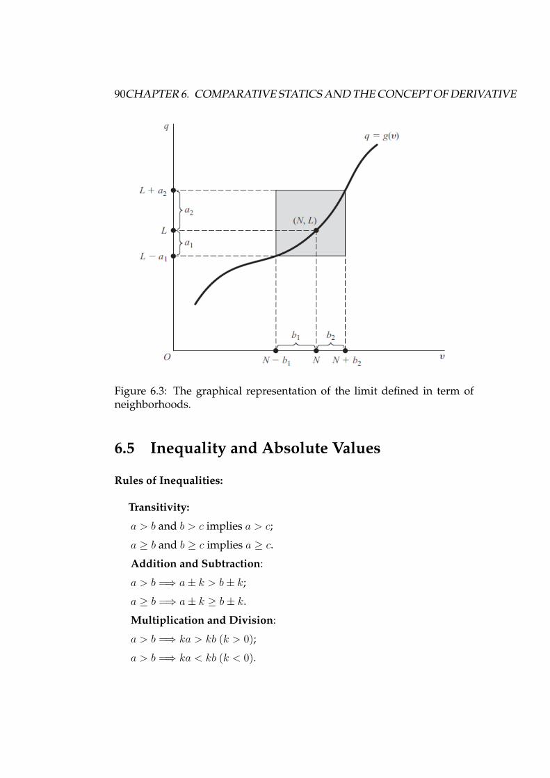
90CHAPTER 6. COMPARATIVE STATICS AND THE CONCEPT OF DERIVATIVE
Figure 6.3: The graphical representation of the limit defined in term ofneighborhoods.
6.5 Inequality and Absolute Values
Rules of Inequalities:
Transitivity:
a > b and b > c implies a > c;
a ≥ b and b ≥ c implies a ≥ c.
Addition and Subtraction:
a > b =⇒ a± k > b± k;
a ≥ b =⇒ a± k ≥ b± k.
Multiplication and Division:
a > b =⇒ ka > kb (k > 0);a > b =⇒ ka < kb (k < 0).
6.5. INEQUALITY AND ABSOLUTE VALUES 91
Squaring:
a > b with b ≥ 0 =⇒ a2 > b2.
Absolute Values and Inequalities
For any real number n, the absolute value of n is defined and denoted
by
|n| =
n if n > 0,−n if n < 0,0 if n = 0.
Thus we can write |x| < n as an equivalent way −n < x < n (n > 0).
Also |x| ≤ n if and only if −n ≤ x ≤ n (n > 0).
The following properties characterize absolute values:
1) |m| + |n| ≥ |m+ n|;
2) |m| · |n| = |m · n|;
3) |m||n| =
∣∣∣mn
∣∣∣.
Solution of an Inequality
Example 6.5.1 Find the solution of the inequality 3x−3 > x+1. By adding
(3 − x) to both sides, we have
3x− 3 + 3 − x > x+ 1 + 3 − x.
Thus, 2x > 4 so x > 2.
Example 6.5.2 Solve the inequality |1 − x| ≤ 3.
From |1 − x| ≤ 3, we have −3 ≤ 1 − x ≤ 3, or −4 ≤ −x ≤ 2. Thus,
4 ≥ x ≥ −2, i.e., −2 ≤ x ≤ 4.

92CHAPTER 6. COMPARATIVE STATICS AND THE CONCEPT OF DERIVATIVE
6.6 Limit Theorems
Theorems Involving a Single Equation
Theorem I: If q = av + b, then limv→N q = aN + b.
Theorem II: If q = g(v) = b, then limv→N q = b.
Theorem III: limv→N vk = Nk.
Example 6.6.1 Given q = 5v + 7, then limv→2 = 5 · 2 + 7 = 17.
Example 6.6.2 q = v3. Find limv→2 q.
By theorem III, we have limv→2 = 23 = 8.
Theorems Involving Two Functions
For two functions q1 = g(v) and q2 = h(v), if limv→N q1 = L1, limv→N q2 =L2, then we have the following theorems:
Theorem IV: limv→N(q1 + q2) = L1 + L2.
Theorem V: limv→N(q1q2) = L1L2.
Theorem VI: limv→Nq1q2
= L1L2
(L2 = 0).
Example 6.6.3 Find limv→01+v2+v .
Since limv→0(1 + v) = 1 and limv→0(2 + v) = 2, so limv→01+v2+v = 1
2 .
Remark 6.6.1 Note thatL1 andL2 represent finite numbers; otherwise the-
orems do not apply.
Limit of a Polynomial Function
limv→N
a0 + a1v + a2v2 + · · · + anv
n = a0 + a1N + a2N2 + · · · + anN
n.
6.7. CONTINUITY AND DIFFERENTIABILITY OF A FUNCTION 93
6.7 Continuity and Differentiability of a Func-
tion
Continuity of a Function
Definition 6.7.1 A function q = g(v) is said to be continuous atN if limv→N q
exists and limv→N g(v) = g(N).
Thus the term continuous involves no less than three requirements: (1)
the point N must be in the domain of the function; (2) limv→N g(v) exists;
and (3) limv→N g(v) = g(N).
Remark 6.7.1 It is important to note that while – in discussing the limit
of a function – the point (N,L) is excluded from consideration, we are no
longer excluding it in defining continuity at point N . Rather, as the third
requirement specifically states, the point (N,L) must be on the graph of
the function before the function can be considered as continuous at point
N .
Polynomial and Rational Functions
From the discussion of the limit of polynomial function, we know that
the limit exists and equals the value of the function at N . Since N is a
point in the domain of the function, we can conclude that any polynomial
function is continuous in its domain. By those theorems involving two
functions, we also know any rational function is continuous in its domain.
Example 6.7.1 q = 4v2
v2+1 .
Then
limv→N
4v2
v2 + 1= limv→N 4v2
limv→N(v2 + 1)= 4N2
N2 + 1.

94CHAPTER 6. COMPARATIVE STATICS AND THE CONCEPT OF DERIVATIVE
Example 6.7.2 The rational function
q = v3 + v2 − 4v − 4v2 − 4
is not defined at v = 2 and v = −2. Since v = 2,−2 are not in the domain,
the function is discontinuous at v = 2 and v = −2, despite the fact that its
limit exists as v → 2 or −2 by noting
q = v3 + v2 − 4v − 4v2 − 4
= v(v2 − 4) + v2 − 4v2 − 4
= (v + 1)(v2 − 4)v2 − 4
= v + 1 (v = 2,−2).
Differentiability of a Function
By the definition of the derivative of a function y = f(x), we know that
f ′(x0) exists at x0 if and only if the lim of ∆y/∆x exists at x = x0 as ∆x → 0,
i.e.,
f ′(x0) = lim∆x→0
∆y∆x
≡ lim∆x→0
f(x0 + ∆x) − f(x0)∆x
(differentiability condition).
On the other hand, the function y = f(x) is continuous at x0 if and only
if
limx→x0
f(x) = f(x0) (continuity condition).
We want to know what is the relationship between the continuity and
differentiability of a function. Now we show the continuity of f is a neces-
sary condition for its differentiability. But this is not sufficient.
Since the notation x → x0 implies x = x0, so x−x0 is a nonzero number,

6.7. CONTINUITY AND DIFFERENTIABILITY OF A FUNCTION 95
it is permissible to write the following identity:
f(x) − f(x0) = f(x) − f(x0)x− x0
(x− x0).
Taking the limit of each side of the above equation as x → x0 yields the
following results:
Left side = limx→x0
(f(x) − f(x0)) = limx→x0
f(x) − f(x0).
Right side = limx→x0
f(x) − f(x0)x− x0
limx→x0
(x− x0)
= f ′(x0) limx→x0
(x− x0) = 0.
Thus limx→x0 f(x) − f(x0) = 0. So limx→x0 f(x) = f(x0) which means
f(x) is continuous at x = x0.
Although differentiability implies continuity, the converse may not be
true. That is, continuity is a necessary, but not sufficient, condition for
differentiability. The following example shows this.
Example 6.7.3 f(x) = |x|.
This function is clearly continuous at x = 0. Now we show that it is
not differentiable at x = 0. This involves the demonstration of a disparity
between the left-side limit and the right-side limit. Since, in considering
the right-side limit x > 0, we have
limx→0+
f(x) − f(0)x− 0
= limx→0+
x
x= lim
x→0+1 = 1.
On the other hand, in considering the left-side limit, x < 0; we have
limx→0−
f(x) − f(0)x− 0
= limx→0−
|x|x
= limx→0−
−xx
= limx→0−
−1 = −1.
96CHAPTER 6. COMPARATIVE STATICS AND THE CONCEPT OF DERIVATIVE
Thus, limx→0∆y∆x does not exist since the left-side limit and the right-
side limit are not the same, which implies that the derivative of y = |x|does not exist at x = 0.

Chapter 7
Rules of Differentiation and Their
Use in Comparative Statics
The central problem of comparative-static analysis, that of finding a rate
of change, can be identified with the problem finding the derivative of a
function y = f(x), provided only a small change in x is being considered.
Before going into comparative-static models, we begin some rules of dif-
ferentiation.
7.1 Rules of Differentiation for a Function of One
Variable
Constant-Function Rule
If y = f(x) = c, where c is a constant, then
dy
dx≡ y′ ≡ f ′ = 0.
97

98CHAPTER 7. RULES OF DIFFERENTIATION AND THEIR USE IN COMPARATIVE STATICS
Proof.
dy
dx= lim
x′→x
f(x′) − f(x)x′ − x
= limx′→x
c− c
x′ − x=x′→x 0 = 0.
We can also write dydx
= dfdx
as
d
dxy = d
dxf.
So we may consider d/dx as an operator symbol.
Power-Function Rule
If y = f(x) = xa where a is any real number −∞ < a < ∞,
d
dxf(x) = axa−1.
Remark 7.1.1 Note that:
(i) If a = 0, thend
dxx0 = d
dx1 = 0.
(ii) If a = 1, then y = x. Thus
dx
dx= 1.
For simplicity, we prove this rule only for the case where a = n, where
n is any positive integer. Since
xn − xn0 = (x− x0)(xn−1 + x0xn−2 + x2
0xn−3 + · · · + xn−1
0 ),
thenxn − xn0x− x0
= xn−1 + x0xn−2 + x2
0xn−3 + · · · + xn−1
0 .

7.1. RULES OF DIFFERENTIATION FOR A FUNCTION OF ONE VARIABLE99
Thus,
f ′(x0) = limx→x0
f(x) − f(x0)x− x0
= limx→x0
xn − xn0x− x0
= limx→x0
xn−1 + x0xn−2 + x2
0xn−3 + · · · + xn−1
0
= xn−10 + xn−1
0 + xn−10 + · · · + xn−1
0
= nxn−10 .
Example 7.1.1 Suppose y = f(x) = x−3. Then y′ = −3x−4.
Example 7.1.2 Suppose y = f(x) =√x. Then y′ = 1
2x− 1
2 . In particular, we
can know that f ′(2) = 12 · 2− 1
2 =√
24 .
Power-Function Rule Generalized
If the function is given by y = cxa, then
dy
dx= df
dx= acxa−1.
Example 7.1.3 Suppose y = 2x. Then
dy
dx= 2x0 = 2.
Example 7.1.4 Suppose y = 4x3. Then
dy
dx= 4 · 3x3−1 = 12x2.
Example 7.1.5 Suppose y = 3x−2. Then
dy
dx= −6x−2−1 = −6x−3.
100CHAPTER 7. RULES OF DIFFERENTIATION AND THEIR USE IN COMPARATIVE STATICS
Common Rules:
f(x) = constant ⇒ f ′(x) = 0;
f(x) = xa(a is constant) ⇒ f ′(x) = axa−1;
f(x) = ex ⇒ f ′(x) = ex;
f(x) = ax(a > 0) ⇒ f ′(x) = ax ln a;
f(x) = ln x ⇒ f ′(x) = 1x
f(x) = loga x(a > 0; a = 1) ⇒ f ′(x) = 1x
loga e = 1x ln a
;
f(x) = sin x ⇒ f ′(x) = cosx;
f(x) = cos x ⇒ f ′(x) = − sin x;
f(x) = tan x ⇒ f ′(x) = 1cos2 x
;
f(x) = ctanx ⇒ f ′(x) = − 1sin2 x
;
f(x) = arcsin x ⇒ f ′(x) = 1√1 − x2
;
f(x) = arccos x ⇒ f ′(x) = − 1√1 − x2
;
f(x) = arctan x ⇒ f ′(x) = 11 − x2 ;
f(x) = arcctanx ⇒ f ′(x) = − 11 − x2 .
We will come back to discuss the exponential function and log func-
tions and their derivatives in Chapter 10.
7.2. RULES OF DIFFERENTIATION INVOLVING TWO OR MORE FUNCTIONS OF THE SAME VARIABLE101
7.2 Rules of Differentiation Involving Two or More
Functions of the Same Variable
Let f(x) and g(x) be two differentiable functions. We have the following
rules:
Sum-Difference Rule:
d
dx[f(x) ± g(x)] = d
dxf(x) ± d
dxg(x) = f ′(x) ± g′(x).
This rule can easily be extended to more functions:
d
dx
[n∑i=1
fi(x)]
=n∑i=1
d
dxfi(x) =
n∑i=1
f ′i(x).
Example 7.2.1d
dx(ax2 + bx+ c) = 2ax+ b.
Example 7.2.2 Suppose a short-run total-cost function is given by c = Q3−4Q2 +10Q+75. Then the marginal-cost function is the limit of the quotient
∆C/∆Q, or the derivative of the C function:
dC
dQ= 3Q2 − 8Q+ 10.
In general, if a primitive function y = f(x) represents a total func-
tion, then the derivative function dy/dx is its marginal function. Since the
derivative of a function is the slope of its curve, the marginal function
should show the slope of the curve of the total function at each point x.
Sometimes, we say a function is smooth if its derivative is continuous.

102CHAPTER 7. RULES OF DIFFERENTIATION AND THEIR USE IN COMPARATIVE STATICS
L’Hopital Rule
We may use the derivatives to find the limit of a continuous function of
which the numerator and denominator approach to zero (or infinity), i.e.,
we have the following L’Hopital rule.
Theorem 7.2.1 (L’Hopital Rule) Suppose that f(x) and g(x) are differentiable
on an open interval (a, b), except possibly at c. If limx→c f(x) = limx→c g(x) = 0or limx→c f(x) = limx→c g(x) = ±∞, g′(x) = 0 for all x in (a, b) with x = c,
and limx→cf ′(x)g′(x)
exists. Then,
limx→c
f(x)g(x)
= limx→c
f ′(x)g′(x)
.
Example 7.2.3
q = v3 + v2 − 4v − 4v2 − 4
.
Note that limv→2 v3 + v2 − 4v − 4 = 0 and limv→2 v
2 − 4 = 0. Then, by
L’Hopital Rule, we have
limv→2
v3 + v2 − 4v − 4v2 − 4
= limv→2
ddv
(v3 + v2 − 4v − 4)ddv
(v2 − 4)
= limv→2
3v2 + 2v − 42v
= 3.
Example 7.2.4
q = 4v + 5v2 + 2v − 3
.
Since limv→∞ 4v + 5 = ∞ and limv→∞ v2 + 2v − 3 = ∞, by L’Hopital Rule,
we then have
limv→∞
4v + 5v2 + 2v − 3
= limv→∞
ddv
(4v + 5)ddv
(v2 + 2v − 3)
= limv→∞
42v + 2
= 0.

7.2. RULES OF DIFFERENTIATION INVOLVING TWO OR MORE FUNCTIONS OF THE SAME VARIABLE103
Product Rule:
d
dx[f(x)g(x)] = f(x) d
dxg(x) + g(x) d
dxf(x)
= f(x)g′(x) + g(x)f ′(x).
Proof.
d
dx[f(x0)g(x0)] = lim
x→x0
f(x)g(x) − f(x0)g(x0)x− x0
= limx→x0
f(x)g(x) − f(x)g(x0) + f(x)g(x0) − f(x0)g(x0)x− x0
= limx→x0
f(x)[g(x) − g(x0)] + g(x0)[f(x) − f(x0)]x− x0
= limx→x0
f(x)g(x) − g(x0)x− x0
+ limx→x0
g(x0)f(x) − f(x0)
x− x0
= f(x0)g′(x0) + g(x0)f ′(x0).
Since this is true for any x = x0, this proves the rule.
Example 7.2.5 Suppose y = (2x+3)(3x2). Let f(x) = 2x+3 and g(x) = 3x2.
Then f ′(x) = 2, g′(x) = 6x. Hence,
d
dx[(2x+ 3)(3x2)] = (2x+ 3)6x+ 3x2 · 2
= 12x2 + 18x+ 6x2
= 18x2 + 18x.
As an extension of the rule to the case of three functions, we have
d
dx[f(x)g(x)h(x)] = f ′(x)g(x)h(x) + f(x)g′(x)h(x) + f(x)g(x)h′(x).

104CHAPTER 7. RULES OF DIFFERENTIATION AND THEIR USE IN COMPARATIVE STATICS
Finding Marginal-Revenue Function from Average-Revenue Function
Suppose that the average-revenue (AR) function is specified by
AR = 15 −Q.
The the total-revenue (TR) function is
TR ≡ AR ·Q = 15Q−Q2.
Then, the marginal-revenue (MR) function is given by
MR ≡ d
dQTR = 15 − 2Q.
In general, if AR = f(Q), then
TR ≡ AR ·Q = Qf(Q).
Thus
MR ≡ d
dQTR = f(Q) +Qf ′(Q).
From this, we can tell relationship between MR and AR. Since
MR − AR = Qf ′(Q),
they will always differ the amount of Qf ′(Q). Also, since
AR ≡ TR
Q= PQ
Q= P,
we can view AR as the inverse demand function for the product of the
firm. If the market is perfectly competitive, i.e., the firm takes the price as
given, then P = f(Q) =constant. Hence f ′(Q) = 0. Thus MR − AR = 0

7.2. RULES OF DIFFERENTIATION INVOLVING TWO OR MORE FUNCTIONS OF THE SAME VARIABLE105
or MR = AR. Under imperfect competition, on the other hand, the AR
curve is normally downward-sloping, so that f ′(Q) < 0. Thus MR < AR.
Quotient Rule
d
dx
[f(x)g(x)
]= f ′(x)g(x) − f(x)g′(x)
g2(x).
We will come back to prove this rule after learning the chain rule.
Example 7.2.6
d
dx
[2x− 3x+ 1
]= 2(x+ 1) − (2x− 3)(1)
(x+ 1)2 = 5(x+ 1)2 .
d
dx
[ 5xx2 + 1
]= 5(x2 + 1) − 5x(2x)
(x2 + 1)2 = 5(1 − x2)(x2 + 1)2 .
d
dx
[ax2 + b
cx
]= 2ax(cx) − (ax2 + b)c
(cx)2 = c(ax2 − b)(cx)2 = ax2 − b
cx2 .
Relationship Between Marginal-Cost and Average-Cost Functions
As an economic application of the quotient rule, let us consider the rate
of change of average cost when output varies.
Given a total cost function C = C(Q), the average cost (AC) function
and the marginal-cost (MC) function are given by
AC ≡ C(Q)Q
(Q > 0),
and
MC ≡ C ′(Q).

106CHAPTER 7. RULES OF DIFFERENTIATION AND THEIR USE IN COMPARATIVE STATICS
Figure 7.1: Graphical representation of relationship between marginal-costand average-cost functions
The rate of change of AC with respect to Q can be found by differenti-
ating AC:
d
dQ
[C(Q)Q
]= C ′(Q)Q− C(Q)
Q2 = 1Q
[C ′(Q) − C(Q)
Q
].
From this it follows that, for Q > 0.
d
dQAC > 0 iff MC(Q) > AC(Q);
d
dQAC = 0 iff MC(Q) = AC(Q);
d
dQAC < 0 iff MC(Q) < AC(Q).
7.3. RULES OF DIFFERENTIATION INVOLVING FUNCTIONS OF DIFFERENT VARIABLES107
7.3 Rules of Differentiation Involving Functions
of Different Variables
Now we consider cases where there are two or more differentiable func-
tions, each of which has a distinct independent variable.
Chain Rule
If we have a function z = f(y), where y is in turn a function of another
variable x, say, y = g(x), then the derivative of z with respect to x is given
bydz
dx= dz
dy· dydx
= f ′(y)g′(x). [ChainRule]
The chain rule appeals easily to intuition. Given a ∆x, there must result
in a corresponding ∆y via the function y = g(x), but this ∆y will in turn
being about a ∆z via the function z = f(y).
Proof. Note that
dz
dx= lim
∆x→0
∆z∆x
= lim∆x→0
∆z∆y
∆y∆x
.
Since ∆x → 0 implies ∆y → 0 which in turn implies ∆z → 0, we then
havedz
dx= dz
dy· dydx
= f ′(y)g′(x). Q.E.D.
In view of the function y = g(x), we can express the function z = f(y)as z = f(g(x)), where the contiguous appearance of the two function sym-
bols f and g indicates that this is a compose function (function of a func-
tion). So sometimes, the chain rule is also called the composite function
rule.
As an application of this rule, we use it to prove the quotient rule.

108CHAPTER 7. RULES OF DIFFERENTIATION AND THEIR USE IN COMPARATIVE STATICS
Let z = y−1 and y = g(x). Then z = g−1(x) = 1/g(x) and
dz
dx= dz
dy· dydx
= − 1y2 g
′(x) = − g′(x)g2(x)
.
Thus,
d
dx
[f(x)g(x)
]= d
dx[f(x) · g−1(x)]
= f ′(x)g−1(x) + f(x) ddx
[g−1(x)]
= f ′(x)g−1(x) + f(x)[− g(x)g2(x)
]
= f ′(x)g(x) − f(x)g′(x)g2(x)
. Q.E.D.
Example 7.3.1 If z = 3y2 and y = 2x+ 5, then
dz
dx= dz
dy
dy
dx= 6y(2) = 12y = 12(2x+ 5).
Example 7.3.2 If z = y − 3 and y = x3, then
dz
dx= dz
dy
dy
dx= 1 · 3x2 = 3x2.
Example 7.3.3 z = (x2 + 3x− 2)17. Let z = y17 and y = x2 + 3x− 2. Then
dz
dx= dz
dy
dy
dx= 17y16 · (2x+ 3)
= 17(x2 + 3x− 2)16(2x+ 3).
Example 7.3.4 Suppose TR = f(Q), where output Q is a function of la-
bor input L, or Q = g(L). Then, by the chain rule, the marginal revenue
product of labor (MRPL) is
MRPL = dR
dL= dR
dQ
dQ
dL= f ′(Q)g′(L) = MR ·MPL,
7.3. RULES OF DIFFERENTIATION INVOLVING FUNCTIONS OF DIFFERENT VARIABLES109
whereMRPL is marginal physical product of labor. Thus the result shown
above constitutes the mathematical statement of the well-known result in
economics that MRPL = MR ·MPL.
Inverse-Function Rule
If a function y = f(x) represents a one-to-one mapping, i.e., if the func-
tion is such that a different value of x will always yield a different value of
y, then the function f will have an inverse function x = f−1(y). Here, the
symbol f−1 is a function symbol which signifies a function related to the
function f ; it does not mean the reciprocal of the function f(x). When x
and y refer specifically to numbers, the property of one-to-one mapping is
seen to be unique to the class of function known as monotonic function.
Definition 7.3.1 A function f is said to be monotonically increasing (de-
creasing) if x1 > x2 implies f(x1) > f(x2) (f(x1) < f(x2)).
In either of these cases, an inverse function f−1 exists.
A practical way of ascertaining the monotonicity of a given function
y = f(x) is to check whether the f ′(x) always adheres to the same algebraic
sign for all values. Geometrically, this means that its slope is either always
upward or always downward.
Example 7.3.5 Suppose y = 5x + 25. Since y′ = 5 for all x, the function
is monotonic and thus the inverse function exists. In fact, it is given by
x = 1/5y − 5.
Generally speaking, if an inverse function exists, the original and the
inverse functions must be both monotonic. Moreover, if f−1 is the inverse
function of f , then f must be the inverse function of f−1. For inverse
functions, the rule of differentiation is
dx
dy= 1
dydx
.

110CHAPTER 7. RULES OF DIFFERENTIATION AND THEIR USE IN COMPARATIVE STATICS
Proof.dx
dy= lim
∆y→0
∆x∆y
= lim∆x→0
1∆y∆x
= 1y′
by noting that ∆y → 0 implies ∆x → 0.
Example 7.3.6 Suppose y = x5 + x. Then
dx
dy= 1
dydx
= 15x4 + 1
.
Example 7.3.7 Given y = ln x, its inverse is x = ey. Thereforedx
dy= 1
1/x=
x = ey.
7.4 Integration (The Case of One Variable)
Let f(x) be a continuous function. The indefinite integral of f (denoted by∫f(x)dx) is defined as
∫f(x)dx = F (x) + C,
where F (x) is such that F ′(x) = f(x), and C is an arbitrary constant.
Rules of Integration
•∫[af(x) + bg(x)]dx = a
∫f(x)dx + b
∫g(x)dx, where a and b are con-
stants (linearity of the integral);
•∫f ′(x)g(x)dx = f(x)g(x) −
∫f(x)g′(x)dx (integration by parts);
•∫f(u(t))du
dtdt =
∫f(u)du (integration by substitution).
7.4. INTEGRATION (THE CASE OF ONE VARIABLE) 111
Some Special Rules of Integration:
∫ f ′(x)f(x)
dx = ln |f(x)| + C;∫ 1xdx = ln |x| + C;∫
exdx = ex + C;∫f ′(x)ef(x)dx = ef(x) + C;∫xadx = xa+1
a+ 1+ C, a = −1;∫
axdx = ax
ln a+ C, a > 0.
Example 7.4.1
∫ x2 + 2x+ 1x
dx =∫xdx+
∫2dx+
∫ 1xdx = x2
2+ 2x+ ln |x| + C.
Example 7.4.2
∫xe−x2
dx = −12
∫(−2x)e−x2
dx = −12
∫e−zdz = −e−x2
2+ C.
Example 7.4.3
∫xexdx = xex −
∫exdx = xex − ex + C.
Definition 7.4.1 (The Newton-Leibniz formula) The definite integral of
a continuous function f is
∫ b
af(x)dx = F (x)|ba = F (b) − F (a)
for F (x) such that F ′(x) = f(x) for all x ∈ [a, b].

112CHAPTER 7. RULES OF DIFFERENTIATION AND THEIR USE IN COMPARATIVE STATICS
Remark 7.4.1 The indefinite integral is a function. The definite integral is
a number.
Properties of Definite Integrals:
∫ b
a[αf(x) + βg(x)]dx = α
∫ b
af(x)dx+ β
∫ b
ag(x)dx;∫ b
af(x)dx = −
∫ a
bf(x)dx;∫ a
af(x)dx = 0;∫ b
af(x)dx =
∫ c
af(x)dx+
∫ b
cf(x)dx;∣∣∣∣∣
∫ b
af(x)dx
∣∣∣∣∣ ≤∫ b
a|f(x)|dx;
∫ b
af(x)g′(x)dx =
∫ g(b)
g(a)f(u)du, u = g(x) (change of variable);∫ b
af ′(x)g(x)dx = f(x)g(x)|ba −
∫ b
af(x)g′(x)dx,
where a, b, c, α, β are real numbers.
Some More Useful Results:
d
dλ
∫ b(λ)
a(λ)f(x)dx = f(b(λ))b′(λ) − f(a(λ))a′(λ).
Example 7.4.4d
dx
∫ x
af(t)dt = f(x).

7.5. PARTIAL DIFFERENTIATION 113
7.5 Partial Differentiation
So far, we considered only the derivative of functions of a single indepen-
dent variable. In comparative-static analysis, however, we are likely to
encounter the situation in which several parameters appear in a model,
so that the equilibrium value of each endogenous variable may be a func-
tion of more than one parameter. Because of this, we now consider the
derivative of a function of more than one variable.
Partial Derivatives
Consider a function
y = f(x1, x2, · · · , xn),
where the variables xi (i = 1, 2, · · · , n) are all independent of one another,
so that each can vary by itself without affecting the others. If the variable
xi changes ∆xi while the other variables remain fixed, there will be a cor-
responding change in y, namely, ∆y. The difference quotient in this case
can be expressed as
∆y∆xi
= f(x1, x2, · · · , xi−1, xi + ∆xi, xi, · · · , xn) − f(x1, x2, · · · , xn)∆xi
.
If we take the limit of ∆y/∆xi, that limit will constitute a derivative.
We call it the partial derivative of y with respect to xi. The process of tak-
ing partial derivatives is called partial differentiation. Denote the partial
derivative of y with respect to xi by ∂y∂xi
, i.e.,
∂y
∂xi= lim
∆xi→0
∆y∆xi
.
Also we can use fi to denote ∂y/∂xi. If the function happens to be

114CHAPTER 7. RULES OF DIFFERENTIATION AND THEIR USE IN COMPARATIVE STATICS
written in terms of unsubscripted variables, such as y = f(u, v, w), one
also uses, fu, fv, fw to denote the partial derivatives.
Techniques of Partial Differentiation
Partial differentiation differs from the previously discussed differen-
tiation primarily in that we must hold the other independent variables
constant while allowing one variable to vary.
Example 7.5.1 Suppose that y = f(x1, x2) = 3x21 + x1x2 + 4x2
2. Find ∂y/∂x1
and ∂y/∂x2.∂y
∂x1≡ ∂f
∂x1= 6x1 + x2;
∂y
∂x2≡ ∂f
∂x2= x1 + 8x2.
Example 7.5.2 For y = f(u, v) = (u+ 4)(3u+ 2v), we have
∂y
∂u≡ fu = (3u+ 2v) + (u+ 4) · 3
= 6u+ 2v + 12;
∂y
∂v≡ fv = 2(u+ 4).
When u = 2 and v = 1, then fu(2, 1) = 26 and fv(2, 1) = 12.
Example 7.5.3 Given y = (3u− 2v)/(u2 + 3v),
∂y
∂u= 3(u2 + 3v) − (3u− 2v)(2u)
(u2 + 3v)2 = −3u2 + 4uv + 9v(u2 + 3v)2 ;
and∂y
∂v= −2(u2 + 3v) − (3u− 2v) · 3
(u2 + 3v)2 = −u(2u+ 9)(u2 + 3v)2 .

7.6. APPLICATIONS TO COMPARATIVE-STATIC ANALYSIS 115
7.6 Applications to Comparative-Static Analysis
Equipped with the knowledge of the various rules of differentiation, we
can at last tackle the problem posed in comparative-static analysis: name-
ly, how the equilibrium value of an endogenous variable will change when
there is a change in any of the exogenous variables or parameters.
Market Model
For the one-commodity market model:
Qd = a− bp (a, b > 0);
Qs = −c+ dp (c, d > 0),
the equilibrium price and quantity are given by
p = a+ c
b+ d;
Q = ad− bc
b+ d.
These solutions will be referred to as being in the reduced form: the
two endogenous variables have been reduced to explicit expressions of
the four independent variables, a, b, c, and d.
To find how an infinitesimal change in one of the parameters will af-
fect the value of p or Q, one has only to find out its partial derivatives. If
the sign of a partial derivative can be determined, we will know the di-
rection in which p will move when a parameter changes; this constitutes
a qualitative conclusion. If the magnitude of the partial derivative can be
ascertained, it will constitute a quantitative conclusion.
Also, to avoid misunderstanding, a clear distinction should be made
between the two derivatives, say, ∂Q/∂a and ∂Qd/∂a. The latter derivative

116CHAPTER 7. RULES OF DIFFERENTIATION AND THEIR USE IN COMPARATIVE STATICS
is a concept appropriate to the demand function taken alone, and without
regard to the supply function. The derivative ∂Q/∂a, on the other hand, to
the equilibrium quantity which takes into account interaction of demand
and supply together. To emphasize this distinction, we refer to the partial
derivatives of p and Qwith respect to the parameters as comparative-static
derivatives.
For instance, for p, we have
∂p
∂a= 1b+ d
;
∂p
∂b= − a+ c
(b+ d)2 ;
∂p
∂c= 1b+ d
;
∂p
∂d= − a+ c
(b+ d)2 .
Thus ∂p∂a
= ∂p∂c> and ∂p
∂b= ∂p
∂d< 0.
National-Income Model
Y = C + I0 +G0 (equilibrium condition);
C = α + β(Y − T ) (α > 0; 0 < β < 1);
T = γ + δY (γ > 0; 0 < δ < 1),
where the endogenous variables are the national income Y , consumption
C, and taxes T . The equilibrium income (in reduced form) is
Y = α− βγ + I0 +G0
1 − β + βδ.

7.6. APPLICATIONS TO COMPARATIVE-STATIC ANALYSIS 117
Figure 7.2: The graphical illustration of comparative statics: (a) increase ina; (b) increase in b; (c) increase in c, and (d) increase in d.
Thus,
∂Y
∂G0= 1
1 − β + βδ> 0 (the government-expenditure multiplier);
∂Y
∂γ= −β
1 − β + βδ< 0;
∂Y
∂δ= −β(α− βγ + I0 +G0)
(1 − β + βδ)2 = −βY(1 − β + βδ)
< 0.

118CHAPTER 7. RULES OF DIFFERENTIATION AND THEIR USE IN COMPARATIVE STATICS
7.7 Note on Jacobian Determinants
Partial derivatives can also provide a means of testing whether there exists
functional (linear or nonlinear) dependence among a set of n variables.
This is related to the notion of Jacobian determinants.
Consider n differentiable functions in n variables not necessary linear.
y1 = f 1(x1, x2, · · · , xn);
y2 = f 2(x1, x2, · · · , xn);
· · · ;
yn = fn(x1, x2, · · · , xn),
where the symbol f i denotes the ith function, we can derive a total of n2
partial derivatives.
∂yi∂xj
(i = 1, 2, · · · , n; j = 1, 2, · · · , n).
We can arrange them into a square matrix, called the Jacobian matrix
and denoted by J , and then take its determinant, the result will be what
is known as a Jacobian determinant (or a Jacobian, for short), denoted by
|J |:
|J | =∣∣∣∣∣ ∂(y1, y2, · · · , yn)∂(x1, x2, · · · , xn)
∣∣∣∣∣ =
∣∣∣∣∣∣∣∣∣∣∣∣∣
∂y1∂x1
∂y1∂x2
· · · ∂y1∂xn
∂y2∂x1
∂y2∂x2
· · · ∂y2∂xn
· · · · · · · · · · · ·∂yn
∂x1
∂yn
∂x2· · · ∂yn
∂xn
∣∣∣∣∣∣∣∣∣∣∣∣∣.
Example 7.7.1 Consider two functions:
y1 = 2x1 + 3x2;

7.7. NOTE ON JACOBIAN DETERMINANTS 119
y2 = 4x21 + 12x1x2 + 9x2
2.
Then the Jacobian determinant is
|J | =
∣∣∣∣∣∣∣∂y1∂x1
∂y1∂x2
∂y2∂x1
∂y2∂x2
∣∣∣∣∣∣∣ =
∣∣∣∣∣∣∣2 3
(8x1 + 12x2) (12x1 + 18x2)
∣∣∣∣∣∣∣ = 0.
A Jacobian test for the existence of functional dependence among a set
of n functions is provided by the following theorem:
Theorem 7.7.1 The n functions f 1, f 2, · · · fn are functionally (linear or non-
linear) dependent if and only if the Jacobian determinant |J | defined above will be
identically zero for all values of x1, x2, · · · , xn.
For the above example, since
|J | =∣∣∣∣∣ ∂(y1, y2)∂(x1, x2)
∣∣∣∣∣ = (24x1 + 36x2) − (24x1 + 36x2) ≡ 0
for all x1 and x2, then y1 and y2 are functionally dependent. In fact, y2 is
simply y1 squared.
Example 7.7.2 Consider the linear-equation system: Ax = d, i.e.,
a11x1 + a12x2 + · · · + a1nxn = d1;
a21x1 + a22x2 + · · · + a2nxn = d2;
· · · ;
an1x1 + an2x2 + · · · + annxn = dn.
We know that the rows of the coefficient matrix A are linearly depen-
dent if and only if |A| = 0. This result can now be interpreted as a special
application of the Jacobian criterion of functional dependence.

120CHAPTER 7. RULES OF DIFFERENTIATION AND THEIR USE IN COMPARATIVE STATICS
To see this, take the left side of each equation Ax = d as a separate
function of the n variables x1, x2, · · · , xn, and denote these functions by
y1, y2, · · · , yn. Then we have ∂yi/∂xj = aij . In view of this, the elements of
|J | will be precisely the elements of A, i.e., |J | = |A| and thus the Jacobian
criterion of functional dependence among y1, y2, · · · , yn is equivalent to the
criterion |A| = 0 in the present linear case.

Chapter 8
Comparative-Static Analysis of
General-Functions
The study of partial derivatives has enables us, in the preceding chap-
ter, to handle the simple type of comparative-static problems, in which
the equilibrium solution of the model can be explicitly stated in the re-
duced form. We note that the definition of the partial derivative requires the
absence of any functional relationship among the independent variables. As ap-
plied to comparative-static analysis, this means that parameters and/or
exogenous variables which appear in the reduced-form solution must be
mutually independent.
However, no such expediency should be expected when, owing to the
inclusion of general functions in a model, no explicit reduced-form solu-
tion can be obtained. In such a case, we will have to find the comparative-
static derivatives directly from the originally given equations in the model.
Take, for instance, a simple national-income model with two endogenous
variables Y and C:
Y = C + I0 +G0 (equilibrim condition);
121
122CHAPTER 8. COMPARATIVE-STATIC ANALYSIS OF GENERAL-FUNCTIONS
C = C(Y, T0) (T0 : exogenous taxes),
which reduces to a single equation
Y = C(Y, T0) + I0 +G0
to be solved for Y . We must, therefore, find the comparative-static deriva-
tives directly from this equation. How might we approach the problem?
Let us suppose that an equilibrium solution Y does exists. We may
write the equation
Y = Y (I0, G0, T0),
even though we are unable to determine explicitly the form which this
function takes. Furthermore, in some neighborhood of Y , the following
identical equality will hold:
Y ≡ C(Y , T0) + I0 +G0.
Since Y is a function of T0, the two arguments of the C function are not
independent. T0 can in this case affect C not only directly, but also indi-
rectly via Y . Consequently, partial differentiation is no longer appropriate
for our purposes. In this case, we must resort to total differentiation (as a-
gainst partial differentiation). The process of total differentiation can lead
us to the related concept of total derivative. Once we become familiar
with these concepts, we shall be able to deal with functions whose argu-
ments are not all independent so that we can study the comparative-static
of a general-function model.

8.1. DIFFERENTIALS 123
8.1 Differentials
The symbol dy/dx has been regarded as a single entity. We shall now rein-
terpret as a ratio of two quantities, dy and dx.
Differentials and Derivatives
Given a function y = f(x), we can use the difference quotient ∆y/∆xto represent the ratio of change of y with respect to x. Since
∆y ≡[
∆y∆x
]∆x, (8.1.1)
the magnitude of ∆y can be found, once the ∆y/∆x and the variation ∆xare known. If we denote the infinitesimal changes in x and y, respectively,
by dx and dy, the identity (8.1) becomes
dy ≡[dy
dx
]dx. (8.1.2)
or
dy = f ′(x)dx. (8.1.3)
The symbols dy and dx are called the differentials of y and x, respec-
tively.
Dividing the two identities in (8.1.2) throughout by dx, we have
(dy)(dx)
≡(dy
dx
).
or(dy)(dx)
≡ f ′(x).
This result shows that the derivative dy/dx ≡ f ′(x) may be interpreted

124CHAPTER 8. COMPARATIVE-STATIC ANALYSIS OF GENERAL-FUNCTIONS
as the quotient of two separate differentials dy and dx.
On the basis of (8.1.2), once we are given f ′(x), dy can immediately be
written as f ′(x)dx. The derivative f ′(x) may thus be viewed as a "convert-
er" that serves to convert an infinitesimal change dx into a corresponding
change dy.
Example 8.1.1 Given y = 3x2 + 7x − 5, find dy. Since f ′(x) = 6x + 7, the
desired differential is
dy = (6x+ 7)dx.
Remark 8.1.1 The purpose of finding the differential dy is called the dif-
ferentiation. Recall that we have also used this term as a synonym for
derivation. To avoid confusion, the word “differentiation" with the phrase
“with respect to x" when we take derivative dy/dx.
The following diagram shows the relationship between “∆y" and “dy":
∆y ≡[
∆y∆x
]∆x = CB
ACAC = CB;
dy =[dy
dx
]∆x = CD
ACAC = CD,
which differs from ∆y by an error of DB.
Differentials and Point Elasticity
As an illustration of the application of differentials in economics, let us
consider the elasticity of a function. For a demand function Q = f(P ), for
instance, the price elasticity of demand is defined as (∆Q/Q)/(∆P/P ), the
ratio of percentage change in quantity demanded and percentage change
in price. Now if ∆P → 0, the ∆P and ∆Q will reduce to the differential

8.1. DIFFERENTIALS 125
dP and dQ, and the elasticity becomes
ϵd ≡ dQ/Q
dP/P= dQ/dP
Q/P= marginal demand function
average demand function.
In general, for a given function y = f(x), the point elasticity of y with
respect to x as
ϵyx = dy/dx
y/x= marginal function
average function.
Example 8.1.2 Find ϵd if the demand function is Q = 100 − 2P . Since
dQ/dP = −2 and Q/P = (100 − 2P )/P , so ϵd = (−P )/(50 − P ). Thus the
demand is inelastic (|ϵd| < 1) for 0 < P < 25, unit elastic (|ϵd| = 1) for
P = 25, and elastic for 25 < P < 50.
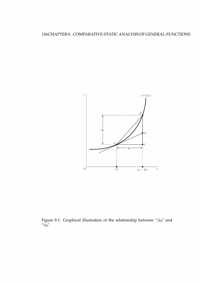
126CHAPTER 8. COMPARATIVE-STATIC ANALYSIS OF GENERAL-FUNCTIONS
Figure 8.1: Graphical illustration of the relationship between “∆y" and“dy".

8.2. TOTAL DIFFERENTIALS 127
8.2 Total Differentials
The concept of differentials can easily be extended to a function of two or
more independent variables. Consider a savings function
S = S(Y, i),
where S is savings, Y is national income, and i is interest rate. If the func-
tion is continuous and possesses continuous partial derivatives, the total
differential is defined by
dS = ∂S
∂YdY + ∂S
∂idi.
That is, the infinitesimal change in S is the sum of the infinitesimal change
in Y and the infinitesimal change in i.
Remark 8.2.1 If i remains constant, the total differential will reduce to the
partial differential:∂S
∂Y=(dS
dY
)i constant
.
Furthermore, general case of a function of n variables y = f(x1, x2, · · · , xn),the total differential of this function is given by
df = ∂f
∂x1dx1 + ∂f
∂x2dx2 + · · · + ∂f
∂xndxn =
n∑i=1
fidxi,
in which each term on the right side indicates the amount of change in y
resulting from an infinitesimal change in one of n variables.
Similar to the case of one variable, the n partial elasticities can be writ-
ten as
ϵfxi= ∂f
∂xi
xif
(i = 1, 2, · · · , n).
128CHAPTER 8. COMPARATIVE-STATIC ANALYSIS OF GENERAL-FUNCTIONS
8.3 Rule of Differentials
Let c be constant and u and v be two functions of the variables x1, x2, · · · , xn.
The the following rules are valid:
Rule I: dc = 0;
Rule II: d(cua) = caua−1du;
Rule III: d(u± v) = du± dv;
Rule IV: d(uv) = vdu+ udv;
Rule V: d(u/v) = 1/v2(vdu− udv).
Example 8.3.1 Find dy of the function y = 5x21+3x2. There are two ways to
find dy. One is the straightforward method by finding ∂f/∂x1 and ∂f/∂x2:
∂f/∂x1 = 10x1 and ∂f/∂x2 = 3, which will then enable us to write
dy = f1dx1 + f2dx2 = 10x1dx1 + 3dx2.
The other way is to use the rules given above by letting u = 5x21 and
v = 3x2;
dy = d(5x21) + d(3x2) (by rule III)
= 10x1dx1 + 3dx2 (by rule II).
Example 8.3.2 Find dy of the function y = 3x21 + x1x
22. Since f1 = 6x1 + x2
2
and f2 = 2x1x2, the desired differential is
dy = (6x1 + x22)dx+ 2x1x2dx2.
8.3. RULE OF DIFFERENTIALS 129
By applying the given rules, the same result can be arrived at
dy = d(3x21) + d(x1x
22)
= 6x1dx1 + x22dx1 + 2x1x2dx2
= (6x1 + x22)dx1 + 2x1x2dx2.
Example 8.3.3 For the function
y = x1 + x2
2x21
f1 = −(x1 + 2x2)2x3
1and f2 = 1
2x21,
then
dy = −(x1 + 2x2)2x3
1dx1 + 1
2x21dx2.
The same result can also be obtained by applying the given rules:
dy = 14x4
1[2x2
1d(x1 + x2) − (x1 + x2)d(2x21)] [by rule V]
= 14x4
1[2x2
1(dx1 + dx2) − (x1 + x2)4x1dx1]
= 14x4
1[−2x1(x1 + 2x2)dx1 + 2x2
1dx2]
= −x1 + 2x2
2x31
dx1 + 12x2
1dx2.
For the case of more than two functions, we have:
Rule VI: d(u± v ± w) = du± dv ± dw;
Rule VII: d(uvw) = vwdu+ uwdv + uvdw.
130CHAPTER 8. COMPARATIVE-STATIC ANALYSIS OF GENERAL-FUNCTIONS
8.4 Total Derivatives
Consider a function
y = f(x,w) with x = g(w).
Unlike a partial derivative, the total derivative does not require the
argument x to main constant as w varies, and can thus allow for the pos-
tulated relationship between the two variables. The variable w can affect y
through two channels: (1) indirectly, via the function g and then f , and (2)
directly, via the function. Whereas the partial derivative fw is adequate for
expressing the direct effect alone, the total derivative is needed to express
both effects jointly.
To get the total derivative, we first get the total differential dy = fxdx+fwdw. Dividing both sides of this equation by dw, we have the total deriva-
tive:
dy
dw= fx
dx
dw+ fw
dw
dw
= ∂y
∂x
dx
dw+ ∂y
∂w.
Example 8.4.1 Find the dy/dw, given the function
y = f(x,w) = 3x− w2 with x = g(w) = 2w2 + w + 4.
dy
dw= fx
dx
dw+ fw = 3(4w + 1) − 2w = 10w + 3.
As a check, we may substitute the function g into f , to get
y = 3(2w2 + w + 4) − w2 = 5w2 + 3w + 12,

8.4. TOTAL DERIVATIVES 131
which is now a function of w alone. Then, we also have
dy
dw= 10w + 3,
and thus we have the identical answer.
Example 8.4.2 Suppose that a utility function is given by
U = U(c, s),
where c is the amount of coffee consumed and s is the amount of sugar
consumed, and another function s = g(c) indicates the complementarity
between these two goods. Then we can find the marginal utility of coffee
given by
MUc = dU
dc= ∂U
∂sg′(c) + ∂U
∂c.
Through the inverse function rule for c = g−1(s), we can also find the
marginal utility of sugar given by
MUs = dU
ds= ∂U
∂c
dc
ds+ ∂U
∂s
= ∂U
∂c
1g′(c)
+ ∂U
∂s.
The marginal rate of substitution of coffee for sugar MRScs is given by
MRScs = MUcMUs
=∂U∂sg′(c) + ∂U
∂c∂U∂c
1g′(c) + ∂U
∂s
= g′(c)[∂U∂sg′(c) + ∂U
∂c∂U∂c
+ ∂U∂sg′(c)
]= g′(c).
A Variation on the Theorem
For a function
y = f(x1, x2, w)
132CHAPTER 8. COMPARATIVE-STATIC ANALYSIS OF GENERAL-FUNCTIONS
with x1 = g(w) and x2 = h(w), the total derivative of y is given by
dy
dw= ∂f
∂x1
dx1
dw+ ∂f
∂x2
dx2
dw+ ∂f
∂w.
Example 8.4.3 Let a production function be
Q = Q(K,L, t),
where K is the capital input, L is the labor input, and t is the time which
indicates that the production can shift over time in reflection of technolog-
ical change. Since capital and labor can also change over time, we may
write
K = K(t) and L = L(t).
Thus the rate of output with respect to time can be denote as
dQ
dt= ∂Q
∂K
dK
dt+ ∂Q
∂L
dL
dt+ ∂Q
∂t.
Another Variation on the Theme
Now if a function is given,
y = f(x1, x2, u, v)
with x1 = g(u, v) and x2 = h(u, v), we can find the total derivative of y
with respect to u (while v is held constant). Since
dy = ∂f
∂x1dx1 + ∂f
∂x2dx2 + ∂f
∂udu+ ∂f
∂vdv,
8.4. TOTAL DERIVATIVES 133
dividing both sides of the above equation by du, we have
dy
du= ∂y
∂x1
dx1
du+ ∂y
∂x2
dx2
du+ ∂y
∂u
du
du+ ∂y
∂v
dv
du
= ∂y
∂x1
dx1
du+ ∂y
∂x2
dx2
du+ ∂y
∂u
[dv
du= 0 since v is constant
].
Since v is held constant, the above is the partial total derivative, we
redenote the above equation by the following notation:
§y§u
= ∂y
∂x1
∂x1
∂u+ ∂y
∂x2
∂x2
∂u+ ∂y
∂u.
Example 8.4.4 Find the partial total derivatives §z§u and §z
§v if
z = 3x2 − 2y4 + 5uv2,
where
x = u− v2 + 4.
and
y = 8u3v + v2 + 1.
By applying the above formula on the partial total derivative, we have
§z§u
= ∂z
∂x
∂x
∂u+ ∂z
∂y
∂y
∂u+ ∂z
∂u
= 6x× 1 − 8y3 × 24u2v + 5v2
= 6x− 196y3u2v + 5v2.

134CHAPTER 8. COMPARATIVE-STATIC ANALYSIS OF GENERAL-FUNCTIONS
and
§z§v
= ∂z
∂x
∂x
∂v+ ∂z
∂y
∂y
∂v+ ∂z
∂v
= 6x× −2v − 8y3 × (8u3 + 2v) + 10uv
= −12xv − 8y3(8u3 + 2v) + 10uv.
Remark 8.4.1 In the cases we have discussed, the total derivative formu-
las can be regarded as expressions of the chain rule, or the composite-
function rule. Also the chain of derivatives does not have to be limited to
only two “links"; the concept of the total derivative should be extendible
to cases where there are three or more links in the composite function.
8.5 Implicit Function Theorem
The concept of total differentials can also enable us to find the derivatives
of the so-called “implicit functions."
Implicit Functions
A function given in the form of y = f(x1, x2, · · · , xn) is called the explicit
function, because the variable y is explicitly expressed as a function of x.
But in many cases y is not an explicit function x1, x2, · · · , xn, instead, the
relationship between y and x1, · · · , xn is given with the form of
F (y, x1, x2, · · · , xn) = 0.
Such an equation may also be defined as implicit function y = f(x1, x2, · · · , xn).Note that an explicit function y = f(x1, x2, · · · , xn) can always be trans-

8.5. IMPLICIT FUNCTION THEOREM 135
formed into an equation
F (y, x1, x2, · · · , xn) ≡ y − f(x1, x2, · · · , xn) = 0.
The reverse transformation is not always possible.
In view of this uncertainty, we have to impose certain conditions under
which we ensure that a given equation F (y, x1, x2, · · · , xn) = 0 does indeed
define an implicit function y = f(x1, x2, · · · , xn). Such a result is given by
the so-called "implicit-function theorem."
Theorem 8.5.1 (Implicit-Function Theorem) Given F (y, x1, x2, · · · , xn) =0, suppose that the following conditions are satisfied:
(a) the function F has continuous partial derivatives Fy, Fx1 , Fx2 , · · · , Fxn ;
(b) at point (y0, x10, x20, · · · , xn0) satisfyingF (y0, x10, x20, · · · , xn0) =0, Fy is nonzero.
Then there exists an n−dimensional neighborhood of x0 = (x10, x20, · · · , xn0),denoted byN(x0), such that y is an implicitly defined function of variables x1, x2, · · · , xn,
in the form of y = f(x1, x2, · · · , xn), and F (y, x1, x2, · · · , xn) = 0 for all points
in N(x0). Moreover, the implicit function f is continuous, and has continuous
partial derivatives f1, · · · , fn.
Derivatives of Implicit Functions
Differentiating F , we have dF = 0, or
Fydy + F1dx1 + · · · + Fndxn = 0.
Suppose that only y and x1 are allowed to vary. Then the above equa-

136CHAPTER 8. COMPARATIVE-STATIC ANALYSIS OF GENERAL-FUNCTIONS
tion reduce to Fydy + F1dx1 = 0. Thus
dy
dx1
∣∣∣∣∣other variable constant≡ ∂y
∂x1= −F1
Fy.
In the simple case where the given equation is F (y, x) = 0, the rule
givesdy
dx= −Fx
Fy.
Example 8.5.1 Suppose y − 3x4 = 0. Then dydx
= −Fx
Fy= −−12x3
1 = 12x3.
In this particular case, we can easily solve the given equation for y, to
get y = 3x4 so that dy/dx = 12x3.
Example 8.5.2 F (x, y) = x2 + y2 − 9 = 0. Thus,
dy
dx= −Fx
Fy= −2x
2y= −x
y, (y = 0).
Example 8.5.3 F (y, x, w) = y3x2 + w3 + yxw − 3 = 0, we have
∂y
∂x= −Fx
Fy= − 2y3x+ yw
3y2x2 + xw.
In particular, at point (1, 1, 1), ∂y∂x
= −3/4.
Example 8.5.4 Suppose that the equation F (Q,K,L) = 0 implicitly de-
fines a production functionQ = f(K,L). Then we can findMPK (marginal
product of labor) and MPL (marginal product of capital) as follows:
MPK ≡ ∂Q
∂K= −FK
FQ;
MPL ≡ ∂Q
∂L= −FL
FQ.
In particular, we can also find theMRTSLK (marginal rate of technical

8.5. IMPLICIT FUNCTION THEOREM 137
substitution) which is given by
MRTSLK ≡ |∂K∂L
| = FLFK
.
Extension to the Simultaneous-Equation Case
Consider a set of simultaneous equations.
F 1(y1, · · · , yn; x1, · · · , xm) = 0;
F 2(y1, · · · , yn; x1, · · · , xm) = 0;
· · ·
F n(y1, · · · , yn;x1, · · · , xm) = 0.
Suppose that F 1, F 2, · · · , F n are differentiable. Taking differentials on
both side of the equation system, we then have
∂F 1
∂y1dy1+∂F 1
∂y2dy2+· · ·+∂F 1
∂yndyn = −
[∂F 1
∂x1dx1 + ∂F 1
∂x2dx2 + · · · + ∂F 1
∂xmdxm
];
∂F 2
∂y1dy1+∂F 2
∂y2dy2+· · ·+∂F 2
∂yndyn = −
[∂F 2
∂x1dx1 + ∂F 2
∂x2dx2 + · · · + ∂F 2
∂xmdxm
];
· · ·
∂F n
∂y1dy1+
∂F n
∂y2dy2+· · ·+∂F
1
∂yndyn = −
[∂F n
∂x1dx1 + ∂F n
∂x2dx2 + · · · + ∂F n
∂xmdxm
].
Or in matrix form,
∂F 1
∂y1∂F 1
∂y2· · · ∂F 1
∂yn
∂F 2
∂y1∂F 2
∂y2· · · ∂F 2
∂yn
· · · · · · · · · · · ·∂Fn
∂y1∂Fn
∂y2· · · ∂Fn
∂yn
dy1
dy2
· · ·dyn
= −
∂F 1
∂x1∂F 1
∂x2· · · ∂F 1
∂xn
∂F 2
∂x1∂F 2
∂x2· · · ∂F 2
∂xn
· · · · · · · · · · · ·∂Fn
∂x1∂Fn
∂x2· · · ∂Fn
∂xn
dx1
dx2
· · ·dxm
.
138CHAPTER 8. COMPARATIVE-STATIC ANALYSIS OF GENERAL-FUNCTIONS
Now suppose that the following Jacobian determinant is nonzero:
|J | =∣∣∣∣∣∂(F 1, F 2, · · · , F n)∂(y1, y2, · · · , yn)
∣∣∣∣∣ =
∣∣∣∣∣∣∣∣∣∣∣∣∣
∂F 1
∂y1∂F 1
∂y2· · · ∂F 1
∂yn
∂F 2
∂y1∂F 2
∂y2· · · ∂F 2
∂yn
· · · · · · · · · · · ·∂Fn
∂y1∂Fn
∂y2· · · ∂Fn
∂yn
∣∣∣∣∣∣∣∣∣∣∣∣∣= 0.
Then, we can obtain total differentials dy = (dy1, dy2, . . . , dyn)′ by in-
verting J .
dy = J−1Fxdx,
where
Fx =
∂F 1
∂x1∂F 1
∂x2· · · ∂F 1
∂xn
∂F 2
∂x1∂F 2
∂x2· · · ∂F 2
∂xn
· · · · · · · · · · · ·∂Fn
∂x1∂Fn
∂x2· · · ∂Fn
∂xn
.
If we want to obtain partial derivatives with respect to xi (i = 1, 2, . . . ,m),
we can let dxt = 0 for t = i. Thus, we have the following equation:
∂F 1
∂y1∂F 1
∂y2· · · ∂F 1
∂yn
∂F 2
∂y1∂F 2
∂y2· · · ∂F 2
∂yn
· · · · · · · · · · · ·∂Fn
∂y1∂Fn
∂y2· · · ∂Fn
∂yn
∂y1∂xi
∂y2∂xi
· · ·∂yn
∂xi
= −
∂F 1
∂xi
∂F 2
∂xi
· · ·∂Fn
∂xi
.
Then, by Cramer’s rule, we have
∂yj∂xi
=|J ij |
|J |(j = 1, 2, · · · , n; i = 1, 2, · · · ,m),
where |J ij | is obtained by replacing the jth column of |J | with
Fxi=[∂F 1
∂xi,∂F 2
∂xi, · · · , ∂F
n
∂xi
]′
.

8.5. IMPLICIT FUNCTION THEOREM 139
Of course, we can find these derivatives by inversing the Jacobian ma-
trix J :
∂y1∂xi
∂y2∂xi
· · ·∂yn
∂xi
= −
∂F 1
∂y1∂F 1
∂y2· · · ∂F 1
∂yn
∂F 2
∂y1∂F 2
∂y2· · · ∂F 2
∂yn
· · · · · · · · · · · ·∂Fn
∂y1∂Fn
∂y2· · · ∂Fn
∂yn
−1
∂F 1
∂xi
∂F 2
∂xi
· · ·∂Fn
∂xi
.
In the compact notation,
∂y
∂xi= −J−1Fxi
.
Example 8.5.5 Let the national-income model be rewritten in the form:
Y − C − I0 −G0 = 0;
C − α− β(Y − T ) = 0;
T − γ − δY = 0.
Then
|J | =
∣∣∣∣∣∣∣∣∣∣∂F 1
∂Y∂F 1
∂C∂F 1
∂T
∂F 2
∂Y∂F 2
∂C∂F 2
∂T
∂F 3
∂Y∂F 3
∂C∂F 3
∂T
∣∣∣∣∣∣∣∣∣∣=
∣∣∣∣∣∣∣∣∣∣1 −1 0
−β 1 β
−δ 0 1
∣∣∣∣∣∣∣∣∣∣= 1 − β + βδ.
Suppose that all exogenous variables and parameters are fixed except
G0. Then we have 1 −1 0
−β 1 β
−δ 0 1
∂Y∂G0
∂C∂G0
∂T∂G0
=
100
.
140CHAPTER 8. COMPARATIVE-STATIC ANALYSIS OF GENERAL-FUNCTIONS
We can solve the above equation for, say, ∂Y /∂G0 which comes out to be
∂Y
∂G0=
∣∣∣∣∣∣∣∣∣∣1 −1 00 1 β
0 0 1
∣∣∣∣∣∣∣∣∣∣|J |
= 11 − β + βδ
.
8.6 Comparative Statics of General-Function Mod-
els
Consider a single-commodity market model:
Qd = Qs, [equilibrium condition];
Qd = D(P, Y0), [∂D/∂P < 0; ∂D/∂Y0 > 0];
Qs = S(P ), [dS/dP > 0],
where Y0 is an exogenously determined income. From this model, we can
obtain a single equation:
D(P, Y0) − S(P ) = 0.
Even though this equation cannot be solved explicitly for the equilib-
rium price P , by the implicit-function theorem, we know that there exists
the equilibrium price P that is the function of Y0:
P = P (Y0),
such that
F (P , Y0) ≡ D(P , Y0) − S(P ) = 0.
It then requires only a straight application of the implicit-function rule
8.7. MATRIX DERIVATIVES 141
to produce the comparative-static derivative, dP /dY0:
dP
dY0= −∂F/∂Y0
∂F/∂P= − ∂D/∂Y0
∂D/∂P − dS/dP> 0.
Since Q = S(P ), thus we have
dQ
dY0= dS
dP
dP
dY0> 0.
8.7 Matrix Derivatives
Matrix derivatives play an important role in economic analysis, especially
in econometrics. If A is n × n non-singular matrix, the derivative of its
determinant with respect to A is given by
∂
∂A|A| = [Cij]
where [Cij] is the matrix of cofactors of A.
Some Useful Formulas
Let a, b be k × 1 vectors and M be a k × k matrix. Then we have:
da′b
db= a;
db′a
db= a;
dMb
db= M ′;
db′Mb
db= (M + M ′)b.
Example 8.7.1 (Find the Least Square Estimator for Multiple Regression Model)

142CHAPTER 8. COMPARATIVE-STATIC ANALYSIS OF GENERAL-FUNCTIONS
Consider the multiple regression model:
y = Xβ + ϵ,
where n × 1 vector y is the dependent variable, X is a n × k matrix of k
explanatory variables with rank(X) = k, β is a k × 1 vector of coefficients
which are to be estimated and ϵ is a n×1 vector of disturbances. We assume
that the matrices of observations X and y are given. Our goal is to find
an estimator b for β using the least squares method. The least squares
estimator of β is a vector b, which minimizes the expression
E(b) = (y − Xb)′(y − Xb) = y′y − y′Xb − b′X ′y + b′X ′Xb.
The first-order condition for extremum is:
dE(b)db
= 0 ⇒ −2X ′y + 2X ′Xb = 0 ⇒ b = (X ′X)−1X ′y.
On the other hand, by the third derivation rule above, we have:
dE2(b)db2 = (2X ′X)′ = 2X ′X.
It will be seen in Chapter 11 that, to check whether the solution b is indeed
a minimum, we need to prove the positive definiteness of the matrix X ′X .
First, notice that X ′X is a symmetric matrix. To prove positive definite-
ness, we take an arbitrary k × 1 vector z, z = 0 and check the following
quadratic form:
z′(X ′X)z = (Xz)′(Xz)
The assumptions rank(X) = k and z = 0 imply Xz = 0. Thus X ′X is
positive definite.

Chapter 9
Optimization: Maxima and
Minima of a Function of One
Variable
The optimization problem is the core issue in economics. Rationality (i.e.,
individuals pursue in maximizing their personal interests in economic sit-
uations) is the most basic behavior assumption about individual decision-
makers in economics and also in practice. The basis of their analysis is
solving optimization problems.
Our attention thus is turned to the study of goal equilibrium, in which
the equilibrium state is defined as the optimal position for a given econom-
ic unit and in which the said economic unit will be deliberately striving for
attainment of that equilibrium. Our primary focus will be on the classical
techniques for locating optimal positions - those using differential calcu-
lus.
143

144CHAPTER 9. OPTIMIZATION: MAXIMA AND MINIMA OF A FUNCTION OF ONE VARIABLE
9.1 Optimal Values and Extreme Values
Economics is by large a science of choice. When an economic project is
to be carried out, there are normally a number of alternative ways of ac-
complishing it. One (or more) of these alternatives will, however, be more
desirable than others from the stand-point of some criterion, and it is the
essence of the optimization problem to choose.
The most common criterion of choice among alternatives in economic-
s is the goal of maximizing something (e.g., utility maximization, profit
maximization) or of minimizing something (e.g., cost minimization). Eco-
nomically, we may categorize such maximization and minimization prob-
lems under general heading of optimization. From a purely mathematical
point of view, the collective term for maximum and minimum is the more
matter-of-fact designation extremum, meaning an extreme value.
In formulating an optimization problem, the first order of business is
to delineate an objective function in which the dependent variable rep-
resents the objects whose magnitudes the economic unit in question can
pick and choose. We shall therefore refer to the independent variables as
choice variables.
Consider a general-form objective function y = f(x). Three specific
cases of functions are depicted in the following Figures:
Remark 9.1.1 The point E and F in (c) are relative relative (or local) ex-
tremum, in the sense that each of these points represents an extremum
in some neighborhood of the point only. We shall continue our discussion
mainly with reference to the search for relative extreme. Since an absolute
(or global) maximum must be either a relative maxima or one of the ends
of the function. Thus, if we know all the relative maxima, it is necessary
only to select the largest of these and compare it with the end points in
order to determine the absolute maximum. Hereafter, the extreme values

9.2. EXISTENCE OF EXTREMUM FOR CONTINUOUS FUNCTION 145
Figure 9.1: The extremum for various functions: (a) constant function; (b)monotonic function, (3) non-monotonic function.
considered will be relative or local ones, unless indicated otherwise.
9.2 Existence of Extremum for Continuous Func-
tion
Let X be a domain of a function f . First, we give the following concepts:
Definition 9.2.1 (Local Optimum) Let f(x) be continuous in a neighbor-
hood U of a point x0. It is said to have a local or relative maximum (resp.
minimum) at x0 if for all x ∈ U, x = x0, f(x) ≤ f(x0) (resp. f(x) ≥ f(x0)).
Definition 9.2.2 (Global Optimum) If f(x∗) = f(x) (resp. f(x∗) > f(x))for all x in the domain X of the function, then the function is said to have
global (unique) maximum at x∗; if f(x∗) 5 f(x) (resp. f(x∗) < f(x)) for
all x in the domain of the function, then the function is said to have global
(unique) minimum at x∗.
A classical conclusion about global optimization is the so-called Weier-
strass theorem.

146CHAPTER 9. OPTIMIZATION: MAXIMA AND MINIMA OF A FUNCTION OF ONE VARIABLE
Proposition 9.2.1 (Weierstrass’s Theorem) Suppose that f is continuous on
a closed and bounded subset X of R1 (or, in the general case, of Rn ). Then f
reaches its maximum and minimum in X , i.e. there exist points m,M ∈ X such
that f(m) ≤ f(x) ≤ f(M), for all x ∈ X . Moreover, the set of maximal (resp.
minimal) points is compact.
In order to easily determine whether a function has an extreme point,
the following gives the method of finding extreme values by differential
method. Generally, there are two types of necessary conditions for the
interior extreme point, that is, the first and second order necessary condi-
tions.
9.3 First-Derivative Test for Relative Maximum
and Minimum
Given a function y = f(x), the first derivative f ′(x) plays a key role in
our search for its extreme values. For smooth functions, an interior rela-
tive extreme values can only occur where f ′(x) = 0, which is a necessary
(but not sufficient) condition for a relative extremum (either maximum or
minimum).
We summarize this as in the following proposition on the necessary
condition for extremum.
Proposition 9.3.1 (Fermat’s Theorem) Suppose that f(x) is differentiable on
X and has a local extremum (minimum or maximum) at an interior point x0 ∈ X .
Then f ′(x0) = 0.
Note that if the first derivative vanishes at some point, it does not imply
that at this point f possesses an extremum. Such an example is f = x3. As
such, we can only state that f has a stationary point. We have some useful
results about stationary points.

9.3. FIRST-DERIVATIVE TEST FOR RELATIVE MAXIMUM AND MINIMUM147
Figure 9.2: The first derivative test: (a) f ′(x0) doest not exist; and (b)f ′(x0) = 0.
Proposition 9.3.2 (Rolle Theorem) Suppose that f is continuous in [a, b], d-
ifferentiable on (a, b) and f(a) = f(b). Then there exists a point c ∈ (a, b) such
that f ′(c) = 0.
From Roll Theorem, we can prove the well-known Mean-Value Theo-
rem, also called Lagrange’s Theorem.
Proposition 9.3.3 (the Mean-Value Theorem or Lagrange’s Theorem) Suppose
that f is continuous on [a, b] and differentiable on (a, b). Then there exists a point
c ∈ (a, b) such that f ′(c) = f(b)−f(a)b−a .
Proof. Let g(x) = f(x) − f(b)−f(a)b−a x. Then, g is continuous in [a, b], dif-
ferentiable on (a, b) and g(a) = g(b). Thus, by Rolle Theorem, there exists
one point c ∈ (a, b) such that g′(c) = 0, and therefore f ′(c) = f(b)−f(a)b−a . �
An variation of the above mean-value theorem is in form of integral
calculus:

148CHAPTER 9. OPTIMIZATION: MAXIMA AND MINIMA OF A FUNCTION OF ONE VARIABLE
Figure 9.3: The Mean-Value Theorem implies that there exists some c inthe interval (a, b) such that the secant joining the endpoints of the interval[a, b] is parallel to the tangent at c.
Theorem 9.3.1 (Mean-Value Theorem of Integral Calculus) Suppose that f :[a, b] → R is continuous on [a, b]. Then there exists a number c ∈ (a, b) such
that ∫ b
af(x)dx = f(c)(b− a).
Proof. Let F (x) =∫ xa f(t)dt. Since f : [a, b] → R is continuous on [a, b],
F (x) is continuous and differentiable on (a, b). Then, by the Mean-Value
Theorem, there is c ∈ (a, b) such that
F (b) − F (a)b− a
= F ′(c) = f(c).
Therefore, we have ∫ b
af(x)dx = f(c)(b− a).
�The second variation of the mean-value theorem is the generalized
mean-value theorem:
Proposition 9.3.4 (Cauchy’s Theorem or the Generalized Mean Value Theorem)
Suppose that f and g are continuous in [a, b] and differentiable in (a, b). Then

9.3. FIRST-DERIVATIVE TEST FOR RELATIVE MAXIMUM AND MINIMUM149
there exists at a point c ∈ (a, b) such that (f(b)−f(a))g′(c) = (g(b)−g(a))f ′(c).
Proof. The case that g(a) = g(b) is easy. So, assume that g(a) = g(b). Define
h(x) = f(x) − f(b) − f(a)g(b) − g(a)
g(x).
Then, applying the Mean-Value Theorem gets the result. �To verify if it has a maximum or minimum, we can use the following
proposition on first-derivative test relative extremum.
Proposition 9.3.5 (First-Derivative Test Relative Extremum) Suppose that
f ′(x0) = 0. Then the value of the function at x0, f(x0), is
(a) a relative maximum if f ′(x) changes its sign from positive to negative from
the immediate left of the point x0 to its immediate right;
(b) a relative minimum if f ′(x) changes its sign from negative to positive from
the immediate left of the point x0 to its immediate right;
(c) not extreme point if f ′(x) has the same sign on some neighborhood.
Example 9.3.1 y = (x− 1)3.
x = 1 is not extreme point even f ′(1) = 0.
Example 9.3.2 y = f(x) = x3 − 12x2 + 36x+ 8.Since f ′(x) = 3x2 − 24x+ 36, to get the critical values, i.e., the values of
the function at x satisfying the condition f ′(x) = 0, we set f ′(x) = 0, and
thus
3x2 − 24x+ 36 = 0.
Its roots are x1 = 2 and x2 = 6. It is easy to verify that f ′(x) > 0 for
x < 2 and f ′(x) < 0 for x > 2. Thus x = 2 is a maximal point and the
corresponding maximum value of the function f(2) = 40. Similarly, we
can verify that x = 6 is a minimal point and f(6) = 8.

150CHAPTER 9. OPTIMIZATION: MAXIMA AND MINIMA OF A FUNCTION OF ONE VARIABLE
Example 9.3.3 Find the relative extremum of the average-cost function
AC = f(Q) = Q2 − 5Q+ 8.
Since f ′(2.5) = 0, f ′(Q) < 0 for Q < 2.5, and f ′(Q) > 0 for Q > 2.5, so
Q = 2.5 is a minimal point.
9.4 Second and Higher Derivatives
Since the first derivative f ′(x) of a function y = f(x) is also a function of x,
we can consider the derivative of f ′(x), which is called the second deriva-
tive. Similarly, we can find derivatives of even higher orders. These will
enable us to develop alternative criteria for locating the relative extremum
of a function.
The second derivative of the function f is denoted by f ′′(x) or d2y/dx2.
If the second derivative f ′′(x) exists for all x values, f(x) is said to be twice
differentiable; if, in addition, f ′′(x) is continuous, f(x) is said to be twice
continuously differentiable.
The higher-order derivatives of f(x) can be similarly obtained and
symbolized along the same line as the second derivative:
f ′′′(x), f (4)(x), · · · , f (n)(x),
ord3y
dx3 ,d4y
dx4 , · · · , dny
dxn.
Remark 9.4.1 dny/dxn can be also written as (dn/dxn)y, where the dn/dxn
part serves as an operator symbol instructing us to take the n-th derivative
with respect to x.
Example 9.4.1 y = f(x) = 4x4 − x3 + 17x2 + 3x− 1.

9.5. SECOND-DERIVATIVE TEST 151
Then
f ′(x) = 16x3 − 3x2 + 34x+ 3;
f ′′(x) = 48x2 − 6x+ 34;
f ′′′(x) = 96x− 6;
f (4)(x) = 96;
f (5)(x) = 0.
Example 9.4.2 Find the first four derivatives of the function
y = g(x) = x
1 + x(x = −1).
g′(x) = (1 + x)−2;
g′′(x) = −2(1 + x)−3;
g′′′(x) = 6(1 + x)−4;
g(4)(x) = −24(1 + x)−5.
Remark 9.4.2 A negative second derivative is consistently reflected in an
inverse U-shaped curve; a positive second derivative is reflected in an U-
shaped curve.
9.5 Second-Derivative Test
Recall the meaning of the first and the second derivatives of a function f.
The sign of the first derivative tells us whether the value of the function
increases (f ′ > 0) or decreases(f ′ < 0), whereas the sign of the second
derivative tells us whether the slope of the function increases (f ′′ > 0)or decreases (f ′′ < 0). This gives us an insight how to verify that at a

152CHAPTER 9. OPTIMIZATION: MAXIMA AND MINIMA OF A FUNCTION OF ONE VARIABLE
stationary point there exists a maximum or minimum. Thus, we have the
following result on the second-derivative test for relative extremum.
Proposition 9.5.1 (Second-Derivative Test for Relative Extremum) Suppose
that f ′(x0) = 0. Then the value of the function at x0, f(x0), will be
(a) a relative maximum if f ′′(x0) < 0;
(b) a relative minimum if f ′′(x0) > 0.
This test is in general more convenient to use than the first-derivative
test, since it does not require us to check the derivative sign to both the left
and right of x.
Example 9.5.1 y = f(x) = 4x2 − x.
Since f ′(x) = 8x− 1 and f ′′(x) = 8, we know f(x) reaches its minimum
at x = 1/8. Indeed, since the function plots as a U-shaped curve, the
relative minimum is also the absolute minimum.
Example 9.5.2 y = g(x) = x3 − 3x2 + 2.
y′ = g′(x) = 3x2 − 6x and y′′ = 6x − 6. Setting g′(x) = 0, we obtain the
critical values x1 = 0 and x2 = 2, which in turn yield the two stationary
values g(0) = 2 (a maximum because g′′(0) = −6 < 0) and g(2) = −2 (a
minimum because g′′(2) = 6 > 0).
Remark 9.5.1 Note that when f ′(x0) = 0, f ′′(x0) < 0 (f ′′(x0) > 0) is a
sufficient condition for a relative maximum (resp. minimum) but not a
necessary condition. However, the condition f ′′(x0) ≤ 0 (f ′′(x0) ≥ 0) is a
necessary (even though not sufficient) for a relative maximum (resp. min-
imum).

9.5. SECOND-DERIVATIVE TEST 153
Condition for Profit Maximization
Let R = R(Q) be the total-revenue function and let C = C(Q) be the
total-cost function, where Q is the level of output. The profit function is
then given by
π = π(Q) = R(Q) − C(Q).
To find the profit-maximizing output level, we need to find Q such that
π′(Q) = R′(Q) − C ′(Q),
or
R′(Q) = C ′(Q), or MR(Q) = MC(Q).
To be sure the first-order condition leads to a maximum, we require
d2π
dQ≡ π′′(Q) − C ′′(Q) < 0.
Economically, this would mean that, if the rate of change of MR is less
than the rate of change of MC at Q, then that output Q will maximize
profit.
Example 9.5.3 Let R(Q) = 1200Q − 2Q2 and C(Q) = Q3 − 61.25Q2 +1528.5Q+ 2000. Then the profit function is
π(Q) = −Q3 + 59.2Q2 − 328.5Q− 2000.
Setting π′(Q) = −3Q2 + 118.5Q − 328.5 = 0, we have Q1 = 3 and
Q2 = 36.5. Since π′′(3) = −18 + 118.5 = 100.5 > 0 and π′′(36.5) = −219 +118.5 = −100.5 < 0, so the profit-maximizing output is Q = 36.5.

154CHAPTER 9. OPTIMIZATION: MAXIMA AND MINIMA OF A FUNCTION OF ONE VARIABLE
9.6 Taylor Series
This section considers the so-called "expansion" of a function y = f(x) into
what is known as the Taylor series (expansion around any point x = x0).
To expand a function y = f(x) around a point x0 means to transform that
function into a polynomial form, in which the coefficients of the various
terms are expressed in terms of the derivative values f ′(x0), f ′′(x0), etc. -
all evaluated at the point of expansion x0.
Proposition 9.6.1 (Taylor’s Theorem) Given an arbitrary function ϕ(x), if we
know the values of ϕ(x0), ϕ′(x0), ϕ′′(x0), etc., then this function can be expanded
around the point x0 as follows:
ϕ(x) = ϕ(x0) + ϕ′(x0)(x− x0) + 12!ϕ′′(x0)(x− x0)2 + · · · + 1
n!ϕ(n)(x0)(x− x0)n +Rn
≡ Pn +Rn,
where Pn represents the nth-degree polynomial andRn denotes a remainder which
can be denoted by the so-called Lagrange form of the remainder:
Rn = ϕ(n+1)(P )(n+ 1)!
(x− x0)n+1
with P being a point between x and x0. Here n! is the "n factorial", defined as
n! ≡ n(n− 1)(n− 2) · · · (3)(2)(1).
Remark 9.6.1 When n = 0, the Talor’s Theorem reduces to the mean-value
theorem that we discussed in Section 9.3:
ϕ(x) = P0 +R0 = ϕ(x0) + ϕ′(P )(x− x0),
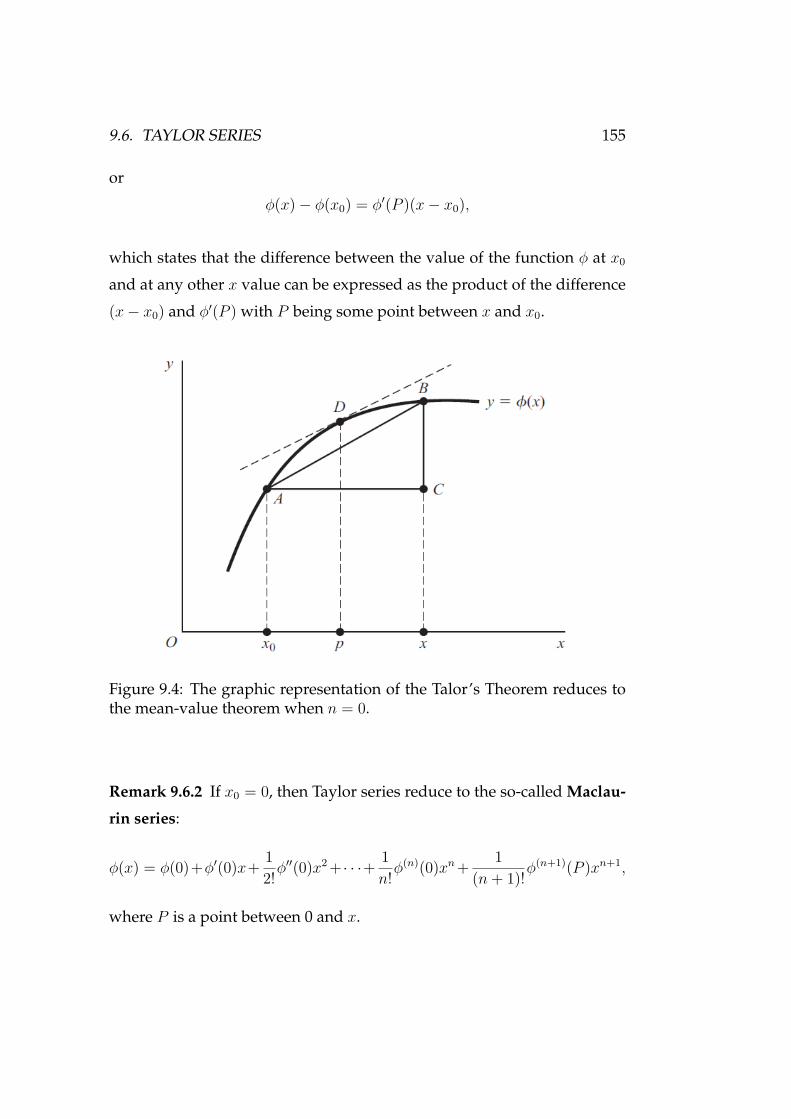
9.6. TAYLOR SERIES 155
or
ϕ(x) − ϕ(x0) = ϕ′(P )(x− x0),
which states that the difference between the value of the function ϕ at x0
and at any other x value can be expressed as the product of the difference
(x− x0) and ϕ′(P ) with P being some point between x and x0.
Figure 9.4: The graphic representation of the Talor’s Theorem reduces tothe mean-value theorem when n = 0.
Remark 9.6.2 If x0 = 0, then Taylor series reduce to the so-called Maclau-
rin series:
ϕ(x) = ϕ(0)+ϕ′(0)x+ 12!ϕ′′(0)x2 + · · ·+ 1
n!ϕ(n)(0)xn+ 1
(n+ 1)!ϕ(n+1)(P )xn+1,
where P is a point between 0 and x.
156CHAPTER 9. OPTIMIZATION: MAXIMA AND MINIMA OF A FUNCTION OF ONE VARIABLE
Example 9.6.1 Expand the function
ϕ(x) = 11 + x
around the point x0 = 1, with n = 4. Since ϕ(1) = 12 and
ϕ′(x) = −(1 + x)−2, ϕ′(1) = −1/4;
ϕ′′(x) = 2(1 + x)−3, ϕ′′(1) = 1/4;
ϕ(3)(x) = −6(1 + x)−4, ϕ(3)(1) = −3/8;
ϕ(4)(x) = 24(1 + x)−5, ϕ(4)(1) = 3/4,
we obtain the following Taylor series:
ϕ(x) = 1/2 − 1/4(x− 1) + 1/8(x− 1)2 − 1/16(x− 1)3 + 1/32(x− 1)4 +Rn.
9.7 Nth-Derivative Test
A relative extremum of the function f can be equivalently defined as fol-
lows:
A function f(x) attains a relative maximum (resp. minimum) value at
x0 if f(x)−f(x0) is nonpositive (resp. nonnegative) for values of x in some
neighborhood of x0.
Assume that f(x) has finite, continuous derivatives up to the desired
order at x = x0, then the function can be expanded around x = x0 as a
Taylor series:
f(x) − f(x0) =f ′(x0)(x− x0) + 12!f ′′(x0)(x− x0)2 + · · ·
+ 1n!f (n)(x0)(x− x0)n + 1
(n+ 1)!f (n+1)(x0)(x− x0)n+1.

9.7. NTH-DERIVATIVE TEST 157
From the above expansion, we have the following proposition.
Proposition 9.7.1 (Nth-Derivative Test) Suppose that f ′(x0) = 0, and the
first nonzero derivative value at x0 encountered in successive derivation is that of
the Nth derivative, f (N)(x0) = 0. Then the stationary value f(x0) will be
(a) a relative maximum if N is an even number and f (N)(x0) < 0;
(b) a relative minimum if N is an even number and f (N)(x0) > 0;
(c) an inflection point if N is odd.
Example 9.7.1 y = (7 − x)4.
Since f ′(7) = 4(7−7)3 = 0, f ′′(7) = 12(7−7)2 = 0, f ′′′(7) = 24(7−7) = 0,
f (n)(7) = 24 > 0, so x = 7 is a minimal point such that f(7) = 0.

158CHAPTER 9. OPTIMIZATION: MAXIMA AND MINIMA OF A FUNCTION OF ONE VARIABLE
Chapter 10
Exponential and Logarithmic
Functions
Exponential functions, as well as the closely related logarithmic functions,
have important applications in economics, especially in connection with
growth problems, and in economic dynamics in general. This chapter dis-
cusses some basic properties and derivatives of exponential and logarith-
mic functions.
10.1 The Nature of Exponential Functions
In this simple version, the exponential function may be represented in the
form:
y = f(t) = bt (b > 1),
where b denotes a fixed base of the exponent t. Its generalized version has
the form:
y = abct.
Remark 10.1.1 y = abct = a(bc)t. Thus we can consider bc as a base of
exponent t. It changes exponent from ct to t and changes base b to bc.
159

160 CHAPTER 10. EXPONENTIAL AND LOGARITHMIC FUNCTIONS
If the base is an irrational number e = 2.71828 · · · , the function:
y = aert
is referred to the natural exponential function, which can be alternatively
denoted as
y = a exp(rt).
Remark 10.1.2 It can be proved that e may be defined as the limit:
e ≡ limn→∞
f(n) = limn→∞
(1 + 1
n
)n.
10.2 Logarithmic Functions
For the exponential function y = bt and the natural exponential function
y = et, taking the log of y to the base b (denote by logb y) and the base e
(denoted by loge y) respectively, we obtain the logarithmic function.
t = logb y,
and
t = loge y ≡ ln y.
For example, we know that 42 = 16. So we can write log4 16 = 2.
Since y = bt ⇐⇒ t = logb y, we can write
blogb y = bt = y.
The following rules are familiar to us:
10.3. DERIVATIVES OF EXPONENTIAL AND LOGARITHMIC FUNCTIONS161
Rules:
(a) ln(uv) = ln u+ ln v (log of product);
(b) ln(u/v) = ln u− ln v (log of quotient);
(c) ln ua = a ln u (log of power);
(d) logb u = (logb e)(loge u) = (logb e)(ln u) (conversion of log
base);
(e) logb e = 1/(loge b) = 1/ ln b (inversion of log base).
Properties of Log:
(a) log y1 = log y2 iff y1 = y2;
(b) log y1 > log y2 iff y1 > y2;
(c) 0 < y < 1 iff log y < 0;
(d) y = 1 iff log y = 0;
(e) log y → ∞ as y → ∞;
(f) log y → −∞ as y → 0.
Remark 10.2.1 t = logb y and t = ln y are the respective inverse functions
of the exponential functions y = bt and y = et.
10.3 Derivatives of Exponential and Logarithmic
Functions
The Basic Rule:
(a) d ln tdt
= 1t;
(b) det
dt= et;
162 CHAPTER 10. EXPONENTIAL AND LOGARITHMIC FUNCTIONS
(c) def(t)
dt= f ′(t)ef(t);
(d) ddt
ln f(t) = f ′(t)f(t) .
Example 10.3.1 The following are examples to find derivatives:
(a) Let y = ert. Then dy/dt = rert;
(b) Let y = e−t. Then dy/dt = −e−t;
(c) Let y = ln at. Then dy/dt = a/at = 1/t;
(d) Let y = ln tc. Since y = ln tc = c ln t, so dy/dt = c(1/t);
(e) Let y = t3 ln t2. Then dy/dt = 3t2 ln t2 + 2t3/t = 2t2(1 + 3 ln t).
The Case of Base b
(a) dbt
dt= bt ln b;
(b) ddt
logb t = 1t ln b ;
(c) ddtbf(t) = f ′(t)bf(t) ln b;
(d) ddt
logb f(t) = f ′(t)f(t)
1ln b .
Proof of (a). Since bt = eln bt = et ln b, then (d/dt)bt = (d/dt)et ln b =(ln b)(et ln b) = bt ln b.
Proof of (b). Since
logb t = (logb e)(loge t) = (1/ ln b) ln t,
(d/dt)(logb t) = (d/dt)[(1/ ln b) ln t] = (1/ ln b)(1/t)
Example 10.3.2 (a) Let y = 121−t. Then dydt
= d(1−t)dt
121−t ln 12 = −121−t ln 12

10.3. DERIVATIVES OF EXPONENTIAL AND LOGARITHMIC FUNCTIONS163
An Application
Example 10.3.3 Find dy/dx from y = xaekx−c. Taking the natural log of
both sides, we have
ln y = a ln x+ kx− c.
Differentiating both sides with respect to x, we get
1y
dy
dx= a
x+ k.
Thus dydx
= (a/x+ k)y = (a/x+ k)xaekx−c.
Use the above technical method, we can similarly find the derivative
of y = ϕψ.

164 CHAPTER 10. EXPONENTIAL AND LOGARITHMIC FUNCTIONS

Chapter 11
Optimization: Maxima and
Minima of a Function of Two or
More Variables
This chapter develops a way of finding the extreme values of an objec-
tive function that involves two or more choice variables. As before, our
attention will be focused heavily on relative extrema, and for this reason
we should often drop the adjective "relative," with the understanding that,
unless otherwise specified, the extrema referred to are relative.
11.1 The Differential Version of Optimization Con-
dition
This section shows the possibility of equivalently expressing the deriva-
tive version of first and second order conditions in terms of differentials.
Consider the function z = f(x). Recall that the differential of z = f(x)is
dz = f ′(x)dx.
165

166CHAPTER 11. OPTIMIZATION: MAXIMA AND MINIMA OF A FUNCTION OF TWO OR MORE VARIABLES
Since f ′(x) = 0, it implies that dz = 0 is the necessary condition for
extreme values. This first-order condition requires that dz = 0 as x is
varied. In such a context, with dx = 0, dz = 0 if and only if f ′(x) = 0.
What about the sufficient conditions in terms of second-order differ-
entials?
Differentiating dz = f ′(x)dx, we have
d2z ≡ d(dz) = d[f ′(x)dx]
= d[f ′(x)]dx
= f ′′(x)dx2.
Note that the symbols d2z and dx2 are fundamentally different. d2z
means the second-order differential of z; but dx2 means the squaring of
the first-order differential dx.
Thus, from the above equation, we have d2z < 0 (resp. d2z > 0) if and
only if f ′′(x) < 0 (resp. f ′′(x) > 0). Therefore, the second-order sufficient
condition for maximum (resp. minimum) of z = f(x) is d2z < 0 (resp.
d2z > 0).
11.2 Extreme Values of a Function of Two Vari-
ables
For a function of one variable, an extreme value is represented graphically
by the peak of a hill or the bottom of a valley in a two-dimensional graph.
With two choice variables, the graph of the function z = f(x, y) becomes a
surface in a 3-space, and while the extreme values are still to be associated
with peaks and bottoms.

11.2. EXTREME VALUES OF A FUNCTION OF TWO VARIABLES 167
Figure 11.1: The graphical illustrations for extrema of the function withtwo choice variables: (a) A is a maximum; and (b) B is a minimum.
First-Order Condition
For a function z = f(x, y), the first-order necessary condition for an
extremum again involves dz = 0 for arbitrary values of dx and dy: an
extremum must be a stationary point, at which z must be constant for
arbitrary infinitesimal changes of two variables x and y.
In the present two-variable case, the total differential is
dz = fxdx+ fydy.
Thus, the equivalent derivative version of the first-order condition dz =0 is
fx = fy = 0 or ∂f/∂x = ∂f/∂y = 0.
As in the earlier discussion, the first-order condition is necessary, but

168CHAPTER 11. OPTIMIZATION: MAXIMA AND MINIMA OF A FUNCTION OF TWO OR MORE VARIABLES
not sufficient. To develop a sufficient condition, we must look to the
second-order total, which is related to second-order partial derivatives.
Second-Order Partial Derivatives
From the function z = f(x, y), we can have two first-order partial
derivatives, fx and fy. Since fx and fy are themselves functions of x, we
can find second-order partial derivatives:
fxx ≡ ∂
∂xfx or
∂2z
∂x2 ≡ ∂
∂x
(∂z
∂x
);
fyy ≡ ∂
∂yfy or
∂2z
∂y2 ≡ ∂
∂y
(∂z
∂y
);
fxy ≡ ∂2z
∂x∂y≡ ∂
∂x
(∂z
∂y
);
fyx ≡ ∂2z
∂y∂x≡ ∂
∂y
(∂z
∂x
).
The last two are called cross (or mixed) partial derivatives.
Theorem 11.2.1 (Schwarz’s Theorem or Young’s Theorem) If at least one
of the two partials is continuous, then
∂2f
∂xj∂xi= ∂2f
∂xi∂xj, i, j = 1, 2, · · · , n.
Remark 11.2.1 Even though fxy and fyx have been separately defined, they
will – according to Young’s theorem, be identical with each other, as long
as the two cross partial derivatives are both continuous. In fact, this the-
orem applies also to functions of three or more variables. Given z =g(u, v, w), for instance, the mixed partial derivatives will be characterized
by guv = gvu, guw = gwu, etc. provided these partial derivatives are contin-
uous.

11.2. EXTREME VALUES OF A FUNCTION OF TWO VARIABLES 169
Example 11.2.1 Find all second-order partial derivatives of z = x3 +5xy−y2. The first partial derivatives of this function are
fx = 3x2 + 5y and fy = 5x− 2y.
Thus, fxx = 6x, fyx = 5, and fyy = −2. As expected, fyx = fxy.
Example 11.2.2 For z = x2e−y, its first partial derivatives are
fx = 2xe−y and fy = −x2e−y.
Again, fyx = fxy.
Second-Order Total Differentials
From the first total differential
dz = fxdx+ fydy,
we can obtain the second-order total differential d2z:
d2z ≡ d(dz) = ∂(dz)∂x
dx+ ∂(dz)∂y
dy
= ∂
∂x(fxdx+ fydy)dx+ ∂
∂y(fxdx+ fydy)dy
= [fxxdx+ fxydy]dx+ [fyxdx+ fyydy]dy
= fxxdx2 + fxydydx+ fyxdxdy + fyydy
2
= fxxdx2 + 2fxydxdy + fyydy
2 [iffxy = fyx].
We know that if f(x, y) satisfy the conditions of Schwarz’s theorem, we
have fxy = fyx.

170CHAPTER 11. OPTIMIZATION: MAXIMA AND MINIMA OF A FUNCTION OF TWO OR MORE VARIABLES
Example 11.2.3 Given z = x3 + 5xy − y2, find dz and dz2.
dz =fxdx+ fydy
=(3x2 + 5y)dx+ (5x− 2y)dy.
d2z =fxxdx2 + 2fxydxdy + fyydy2
=6xdx2 + 10dxdy − 2dy2.
Note that the second-order total differential can be written in matrix
form
d2z = fxxdx2 + 2fxydxdy + fyydy
2
=[dx, dy
] fxx fxy
fyx fyy
dxdy
for the function z = f(x, y), where the matrix
H =
fxx fxy
fyx fyy
is called the Hessian matrix (or simply a Hessian).
Then, by the discussion on quadratic forms in Chapter 5, we have
(a) d2z is positive definite iff fxx > 0 and |H| = fxxfyy−(fxy)2 >
0;
(b) d2z is negative definite iff fxx < 0 and |H| = fxxfyy−(fxy)2 >
0.
From the inequality fxxfyy − (fxy)2 > 0, it implies that fxx and fyy are
required to take the same sign.

11.2. EXTREME VALUES OF A FUNCTION OF TWO VARIABLES 171
Example 11.2.4 Give fxx = −2, fxy = 1, and fyy = −1 at a certain point on
a function z = f(x, y), does d2z have a definite sign at that point regardless
of the values of dx and dy? The Hessian determinant is in this case
∣∣∣∣∣∣∣−2 11 −1
∣∣∣∣∣∣∣ ,with principal minors |H1| = −2 < 0 and
|H2| =
∣∣∣∣∣∣∣−2 11 −1
∣∣∣∣∣∣∣ = 2 − 1 = 1 > 0.
Thus d2z is negative definite.
Using the concept of d2z, we then have:
(a) For maximum of z = f(x, y): d2z < 0 for any values of dx
and dy, not both zero;
(b) For minimum of z = f(x, y): d2z > 0 for any values of dx
and dy, not both zero.
Example 11.2.5 Give fxx = −2, fxy = 1, and fyy = −1 at a certain point on
a function z = f(x, y), does d2z have a definite sign at that point regardless
of the values of dx and dy? The Hessian determinant is in this case
∣∣∣∣∣∣∣−2 11 −1
∣∣∣∣∣∣∣ ,with principal minors |H1| = −2 < 0 and
|H2| =
∣∣∣∣∣∣∣−2 11 −1
∣∣∣∣∣∣∣ = 2 − 1 = 1 > 0.
172CHAPTER 11. OPTIMIZATION: MAXIMA AND MINIMA OF A FUNCTION OF TWO OR MORE VARIABLES
Thus d2z is negative definite.
For operational convenience, second-order differential conditions can
be translated into equivalent conditions on second-order derivatives. The
actual translation would require a knowledge of quadratic forms, which
has already been discussed in Chapter 5.
Second-Order Sufficient Condition for Extremum
For any values of dx and dy, not both zero,
d2z < 0 iff fxx < 0; fyy < 0; and fxxfyy > (fxy)2;
d2z > 0 iff fxx > 0; fyy > 0; and fxxfyy > (fxy)2.
Thus, from the above first- and second-order conditions, we obtain the
following proposition for relative extremum.
Proposition 11.2.1 (Conditions for Extremum) Suppose that z = f(x, y) are
twice continuously differentiable. Then, we have
Conditions for Maximum:
(1) fx = fy = 0 (necessary condition);
(2) fxx < 0; fyy < 0; and fxxfyy > (fxy)2.
Conditions for Minimum:
(1) fx = fy = 0 (necessary condition);
(2) fxx > 0; fyy > 0; and fxxfyy > (fxy)2.
Example 11.2.6 Find the extreme values of z = 8x3 + 2xy − 3x2 + y2 + 1.
fx = 24x2 + 2y − 6x, fy = 2x+ 2y;
11.3. OBJECTIVE FUNCTIONS WITH MORE THAN TWO VARIABLES173
fxx = 48x− 6, fyy = 2, fxy = 2.
Setting fx = 0 and fy = 0, we have
24x2 + 2y − 6x = 0;
2y + 2x = 0.
Then y = −x and thus from 24x2 + 2y − 6y, we have 24x2 − 8x = 0which yields two solutions for x: x1 = 0 and x2 = 1/3.
Since fxx(0, 0) = −6 and fyy(0, 0) = 2, it is impossible fxxfyy ≥ (fxy)2 =4, so the point (x1, y1) = (0, 0) is not extreme point. For the solution
(x2, y2) = (1/3,−1/3), we find that fxx = 10 > 0, fyy = fxy = 2 > 0, and
fxxfyy − (fxy)2 = 20 − 4 > 0, so (x, y, z) = (1/3,−1/3, 23/27) is a relative
minimum point.
Example 11.2.7 z = x + 2ey − ex − e2y. Letting fx = 1 − ex = 0 and
fy = 2e − 2e2y = 0, we have x = 0 and y = 1/2. Since fxx = −ex, fyy =−4e2y, and fxy = 0, then fxx(0, 1/2) = −1 < 0, fyy(0, 1/2) = −4e < 0, and
fxxfyy − (fxy)2 > 0, so (x, y, z) = (0, 1/2,−1) is the maximization of the
function.
11.3 Objective Functions with More than Two Vari-
ables
When there are n choice variables, the objective function may be expressed
as
z = f(x1, x2, · · · , xn).

174CHAPTER 11. OPTIMIZATION: MAXIMA AND MINIMA OF A FUNCTION OF TWO OR MORE VARIABLES
The total differential will then be
dz = f1dx1 + f2dx2 + · · · + fndxn
so that the necessary condition for extremum is dz = 0 for arbitrary dxi,
which in turn means that all the n first-order partial derivatives are re-
quired to be zero:
f1 = f2 = · · · = fn = 0.
It can be verified that the second-order differential d2z can be written
as
d2z =[dx1, dx2, · · · , dxn
]
f11 f12 · · · f1n
f21 f22 · · · f2n
· · · · · · · · · · · ·fn1 fn2 · · · fnn
dx1
dx2
· · ·dxn
≡ (dx)′Hdx.
Thus the Hessian determinant is
|H| =
∣∣∣∣∣∣∣∣∣∣∣∣∣
f11 f12 · · · f1n
f21 f22 · · · f2n
· · · · · · · · · · · ·fn1 fn2 · · · fnn
∣∣∣∣∣∣∣∣∣∣∣∣∣and the second-order sufficient condition for extremum is, as before, that
all the n principal minors be positive for a minimum in z and that they
duly alternate in sign for a maximum in z, the first one being negative.
In summary, we have the following proposition.
Proposition 11.3.1 (Conditions for Extremum) Suppose that z = f(x1, x2, . . . , xn)are twice continuously differentiable. Then, we have:

11.3. OBJECTIVE FUNCTIONS WITH MORE THAN TWO VARIABLES175
Conditions for Maximum:
(1) f1 = f2 = · · · = fn = 0 (necessary condition);
(2) |H1| < 0, |H2| > 0, |H3| < 0, · · · , (−1)n|Hn| > 0. [d2z is
negative definite].
Conditions for Minimum:
(1) f1 = f2 = · · · = fn = 0 (necessary condition);
(2) |H1| > 0, |H2| > 0, |H3| > 0, · · · , |Hn| > 0. [d2z is positive
definite].
Example 11.3.1 Find the extreme values of
z = 2x21 + x1x2 + 4x2
2 + x1x3 + x23 + 2.
From the first-order condition:
f1 = 0 : 4x1 + x2 + x3 = 0;
f2 = 0 : x1 + 8x2 + 0 = 0;
f3 = 0 : x1 + 0 + 2x3 = 0,
we can find a unique solution x1 = x2 = x3 = 0. This means that there is
only one stationary value, z = 2. The Hessian determinant of this function
is
|H| =
∣∣∣∣∣∣∣∣∣∣f11 f12 f13
f21 f22 f23
f31 f32 f33
∣∣∣∣∣∣∣∣∣∣=
∣∣∣∣∣∣∣∣∣∣4 1 11 8 01 0 2
∣∣∣∣∣∣∣∣∣∣.
Since the principal minors of which are all positive: |H1| = 4, |H2| =31, and |H3| = 54, we can conclude that z = 2 is a minimum.

176CHAPTER 11. OPTIMIZATION: MAXIMA AND MINIMA OF A FUNCTION OF TWO OR MORE VARIABLES
11.4 Second-Order Conditions in Relation to Con-
cavity and Convexity
11.4.1 Concavity and Convexity
Second-order conditions which are always concerned with whether a s-
tationary point is the peak of a hill or the bottom of a valley are closely
related to the so-called (strictly) concave or convex functions.
A function that gives rise to a hill (resp. valley) over the entire domain
is said to be a concave (resp. convex) function. If the hill (resp. valley)
pertains only to a subset S of the domain, the function is said to be concave
(resp. convex) on S.
Mathematically, a function is said to be concave (resp. convex) if, for
any pair of distinct points u and v in the domain of f , and for any 0 < θ <
1,
θf(u) + (1 − θ)f(v) ≤ f(θu + (1 − θ)v)
(resp. θf(u) + (1 − θ)f(v) ≥ f(θu + (1 − θ)v))
Further, if the weak inequality "≤" (resp. "≥") is replaced by the strictly
inequality "<" (resp. ">"), the function is said to be strictly concave (resp.
strictly convex).
Remark 11.4.1 θu + (1 − θ)v consists of line segments between points u
and v when θ takes values of 0 ≤ θ ≤ 1. Thus, in the sense of geometry, the
function f is concave (resp. convex) if and only if the line segment of any
two points u and v lies on or below (resp. above) the surface. The function
is strictly concave (resp. strictly convex) if and only if the line segment lies
entirely below (resp. above) the surface, except at M and N .
From the definition of concavity and convexity, we have the following
three theorems:

11.4. SECOND-ORDER CONDITIONS IN RELATION TO CONCAVITY AND CONVEXITY177
Figure 11.2: The graphical illustration of a concave function with twochoice variables and the definition of concavity.
Theorem I (Linear functions). If f(x) is a linear function, then it is a
concave function as well as a convex function, but not strictly so.
Theorem II (Negative of a function). If f(x) is a (strictly) concave
function, then −f(x) is a (strictly) convex function, and vice versa.
Theorem III (Sum of functions). If f(x) and g(x) are both concave
(resp. convex) functions, then f(x)+g(x) is a concave (resp. convex) func-
tion. Further, in addition, either one or both of them are strictly concave
(resp. strictly convex), then f(x) + g(x) is strictly concave (resp. convex).
In view of the association of concavity (resp. convexity) with a global

178CHAPTER 11. OPTIMIZATION: MAXIMA AND MINIMA OF A FUNCTION OF TWO OR MORE VARIABLES
hill (valley) configuration, an extremum of a concave (resp. convex) func-
tion must be a peak - a maximum (resp. a bottom - a minimum). Moreover,
the maximum (resp. minimum) must be a peak an absolute maximum (re-
sp. minimum). Furthermore, the maximum (resp. minimum) is unique if
the function is strictly concave (resp. strictly convex).
In the preceding paragraph, the properties of concavity and convexi-
ty are taken to be global in scope. If they are valid only for a portion of
surface (only in a subset S of domain), the associated maximum and min-
imum are relative to that subset of the domain.
We know that when z = f(x1, · · · , xn) is twice continuous differen-
tiable, z = f(x1, · · · , xn) reaches its maximum (resp. minimum) if d2z is
negative (resp. positive) definite.
The following proposition shows the relationship between concavity
(resp. convexity) and negative definiteness.
Proposition 11.4.1 A twice continuously differentiable function z = f(x1, x2, · · · , xn)is concave (resp. convex) if and only if d2z is everywhere negative (resp. positive)
semidefinite. The said function is strictly concave (resp. convex) if (but not on-
ly if) d2z is everywhere negative (resp. positive) definite, i.e., its Hessian matrix
H = D2f(x) is negative (positive) definite on X .
Remark 11.4.2 As discussed above, the strict concavity of a function f(x)can be determined by testing whether the principal minors of the Hessian

11.4. SECOND-ORDER CONDITIONS IN RELATION TO CONCAVITY AND CONVEXITY179
matrix change signs alternately, namely,
|H1| = f11 > 0,
|H2| =
∣∣∣∣∣∣∣f11 f12
f21 f22
∣∣∣∣∣∣∣ > 0,
|H3| =
∣∣∣∣∣∣∣∣∣∣f11 f12 f13
f21 f22 f23
f31 f32 f33
∣∣∣∣∣∣∣∣∣∣< 0,
· · · ,
(−1)n|Hn| = (−1)n|H| > 0.
and so on, where fij = ∂2f
∂xi∂xj. This algebraic condition is very useful for
testing second-order conditions of optimality. It can easily verify whether
a function is strictly concave (resp. strictly convex) by checking whether
its Hessian matrix is negative (resp. positive) definite.
Example 11.4.1 Check z = −x4 for concavity or convexity by the deriva-
tive condition.
Since d2z = −12x2 ≤ 0 for all x, it is concave. This function, in fact, is
strictly concave.
Example 11.4.2 Check z = x21 + x2
2 for concavity or convexity.
Since
|H| =
∣∣∣∣∣∣∣f11 f12
f21 f22
∣∣∣∣∣∣∣ =
∣∣∣∣∣∣∣2 00 2
∣∣∣∣∣∣∣ ,|H1| = 2 > 0, |H2| = 4 > 0. Thus, by the proposition, the function is
strictly convex.

180CHAPTER 11. OPTIMIZATION: MAXIMA AND MINIMA OF A FUNCTION OF TWO OR MORE VARIABLES
Example 11.4.3 Check if the following production is concave:
Q = f(L,K) = LαKβ,
where L,K > 0; α, β > 0, and α + β < 1.
Since
fL = αLα−1Kβ,
fK = βLαLβ−1;
fLL = α(α− 1)Lα−2Kβ,
fKK = β(β − 1)LαKβ−2,
fLK = αβLα−1Kβ−1,
thus
|H1| = fLL = α(α−)Lα−2Kβ < 0;
|H2| =
∣∣∣∣∣∣∣fLL fLK
fKL fKK
∣∣∣∣∣∣∣ = fLLfKK − (fLK)2
= αβ(α− 1)(β − 1)L2(α−1)K2(β−1) − α2β2L2(α−1)K2(β−1)
= αβ[(α− 1)(β − 1) − αβ]L2(α−1)K2(β−1)
= αβ(1 − α− β)L2(α−1)K2(β−1) > 0.
Therefore, it is strictly concave for L,K > 0, α, β > 0, and α + β < 1.
If we only require a function be differentiable, but not twice differen-
tiable, the following position fully characterizes the concavity of the func-
tion.
Proposition 11.4.2 Suppose that f : R → R is differentiable. Then f is concave

11.4. SECOND-ORDER CONDITIONS IN RELATION TO CONCAVITY AND CONVEXITY181
if and only if for any x, y ∈ R, we have
f(y) 5 f(x) + f ′(x)(y − x). (11.4.1)
Indeed, for a concave function, the from Figure 11.3, we have
u(x) − u(x∗)x− x∗ 5 u′(x∗),
which means (12.5.3).
x* x
slope=u’(x*)
slope=u’(x)-u’(x*)x-x*
Figure 11.3: The graphical illustration why Proposition 11.4.2 holds for aconcave function.
When there are two or more independent variables, the above propo-
sition becomes:
Proposition 11.4.3 Suppose that f : Rn → R is differentiable. Then f is con-

182CHAPTER 11. OPTIMIZATION: MAXIMA AND MINIMA OF A FUNCTION OF TWO OR MORE VARIABLES
cave if and only if for any x,y ∈ R, we have
f(y) 5 f(x) +n∑j=1
∂f(x)∂xj
(yj − xj). (11.4.2)
11.4.2 Concavity/Convexity and Global Optimization
A local optimum is, in general, not equal to the global optimum, but under
certain conditions, these two are consistent with each other.
Theorem 11.4.1 (Global Optimum) Suppose that f is a concave and twice
continuously differentiable function on X ⊆ Rn, and x∗ is an interior point
of X . Then, the following three statements are equivalent:
(1) Df(x∗) = 0.
(2) f has a local maximum at x∗.
(3) f has a global maximum at x∗.
PROOF. It is clear that (3) ⇒ (2), and it follows from the first-order
condition that (2) ⇒ (1). Therefore, we just need to prove that (1) ⇒ (3).
Suppose Df(x∗) = 0. Then f is concave implies that for all x in the
domain, we have:
f(x) 5 f(x∗) +Df(x∗)(x − x∗).
These two formulas mean that for all x, we must have
f(x) 5 f(x∗).
Therefore, f reaches a global maximum at x∗. 2
Theorem 11.4.2 (Uniqueness of Global Optimum) Let X ⊆ Rn.

11.4. SECOND-ORDER CONDITIONS IN RELATION TO CONCAVITY AND CONVEXITY183
(1) If a strictly concave function f defined on X reaches a local max-
imum value at x∗, then x∗ is the unique global maximum point.
(2) If a strictly convex function f reaches a local minimum value at
x, then x is the unique global minimum point.
PROOF. Proof by contradiction. If x∗ is a global maximum point of
function f , but not unique, then there is a point x′ = x∗, such that f(x′) =f(x∗). Suppose that xt = tx′ + (1 − t)x∗. Then, strict concavity requires
that for all t ∈ (0, 1),
f(xt) > tf(x′) + (1 − t)f(x∗).
Since f(x′) = f(x∗),
f(xt) > tf(x′) + (1 − t)f(x′) = f(x′).
This contradicts the assumption that x′ is a global maximum point off .
Consequently, the global maximum point of a strictly concave function is
unique. The proof of part (2) is similar, and thus omitted. 2
Theorem 11.4.3 (The sufficient condition for the uniqueness of global optimum)
Suppose that f(x) is twice continuously differentiable on X ⊆ Rn. We have:
(1) If f(x) is strictly concave and fi(x∗) = 0, i = 1, · · · , n, then x∗
is a unique global maximum point of f(x).
(2) If f(x) is strictly convex and fi(x) = 0, i = 1, · · · , n, then x is a
unique global minimum point of f(x).
184CHAPTER 11. OPTIMIZATION: MAXIMA AND MINIMA OF A FUNCTION OF TWO OR MORE VARIABLES
11.5 Economic Applications
Problem of a Multiproduct Firm
Example 11.5.1 Suppose that a competitive firm produces two products.
Let Qi represents the output level of the i-th product and let the prices of
the products are denoted by P1 and P2. Since the firm is a competitive
firm, it takes the prices as given. Accordingly, the firm’s revenue function
will be
TR = P1Q1 + P2Q2
The firm’s cost function is assumed to be
C = 2Q21 +Q1Q2 + 2Q2
2.
Then, the profit function of this hypothetical firm is given by
π = TR − C = P1Q1 + P2Q2 − 2Q21 −Q1Q2 − 2Q2
2.
The firm wants to maximize the profit by choosing the levels of Q1 and
Q2. For this purpose, setting
∂π
∂Q1= 0 : 4Q1 +Q2 = P1;
∂π
∂Q2= 0 : Q1 + 4Q2 = P2,
we have
Q1 = 4P1 − P2
15and Q2 = 4P2 − P1
15.
Also the Hessian matrix is
H =
π11 π12
π21 π22
=
−4 −1−1 −4
.

11.5. ECONOMIC APPLICATIONS 185
Since |H1| = −4 < 0 and |H2| = 16 − 1 > 0, the Hessian matrix (or
d2z) is negative definite, and the solution does maximize. In fact, since
H is everywhere negative definite, the maximum profit found above is
actually a unique absolute maximum.
Example 11.5.2 Let us now transplant the problem in the above example
into the setting of a monopolistic market.
Suppose that the demands facing the monopolist firm are as follows:
Q1 = 40 − 2P1 + P2;
Q2 = 15 + P1 − P2.
Again, the cost function is given by
C = Q21 +Q1Q2 +Q2
2.
From the monopolistic’s demand function, we can express prices P1
and P2 as functions of Q1 and Q2 and so for the profit function. That is,
solving
− 2P1 + P2 = Q1 − 40;
P1 − P2 = Q2 − 15,
we have
P1 = 55 −Q1 −Q2;
P2 = 70 −Q1 − 2Q2.

186CHAPTER 11. OPTIMIZATION: MAXIMA AND MINIMA OF A FUNCTION OF TWO OR MORE VARIABLES
Consequently, the firm’s total revenue function TR can be written as
TR =P1Q1 + P2Q2
=(55 −Q1 −Q2)Q1 + (70 −Q1 − 2Q2)Q2;
=55Q1 + 70Q2 − 2Q1Q2 −Q21 − 2Q2
2.
Thus the profit function is
π = TR − C
= 55Q1 + 70Q2 − 3Q1Q2 − 2Q21 − 3Q2
2,
which is an object function with two choice variables Q1 and Q2. Setting
∂π
∂Q1= 0 : 4Q1 + 3Q2 = 55;
∂π
∂Q2= 0 : 3Q1 + 6Q2 = 70,
we can find the solution output level are
(Q1, Q2) = (8, 723
).
The prices and profit are
P1 = 3913, P2 = 462
3, and π = 4881
3.
Inasmuch as the Hessian determinant is∣∣∣∣∣∣∣−4 −3−3 −6
∣∣∣∣∣∣∣ ,we have |H1| = −4 < 0 and |H2| = 15 > 0 so that the value of π does rep-
resent the maximum. Also, since Hessian matrix is everywhere negative

11.5. ECONOMIC APPLICATIONS 187
definite, it is a unique absolute maximum.

188CHAPTER 11. OPTIMIZATION: MAXIMA AND MINIMA OF A FUNCTION OF TWO OR MORE VARIABLES

Chapter 12
Optimization with Equality
Constraints
The last chapter presented a general method for finding the relative ex-
trema of an objective function of two or more variables. One important
feature of that discussion is that all the choice variables are independent
of one another, in the sense that the decision made regarding one vari-
able does not depend on the choice of the remaining variables. However,
in many cases, optimization problems are the constrained optimization
problem. For instance, every consumer maximizes her utility subject to
her budget constraint. A firm minimizes the cost of production with the
constraint of production technique.
In the present chapter, we shall consider the problem of optimization
with equality constraints. Our primary concern will be with relative con-
strained extrema.
189

190 CHAPTER 12. OPTIMIZATION WITH EQUALITY CONSTRAINTS
12.1 Effects of a Constraint
In general, for a function, say z = f(x, y), the difference between a con-
strained extremum and a free extremum may be illustrated in Figure 12.1.
Figure 12.1: Difference between a constrained extremum and a free ex-tremum
The free extremum in this particular graph is the peak point of entire
domain, but the constrained extremum is at the peak of the inverse U-
shaped curve situated on top of the constraint line. In general, a constraint
(less freedom) maximum can be expected to have a lower value than the
free (more freedom) maximum, although by coincidence, the two maxi-

12.2. FINDING THE STATIONARY VALUES 191
ma may happen to have the same value. But the constrained maximum
can never exceed the free maximum. To have certain degrees of freedom
of choices, the number of constraints in general should be less than the
number of choice variables.
12.2 Finding the Stationary Values
For illustration, let us consider a consumer choice problem: maximize her
utility:
u(x1, x2) = x1x2 + 2x1
subject to the budget constraint:
4x1 + 2x2 = 60.
Even without any new technique of solution, the constrained maxi-
mum in this problem can easily be found. Since the budget line implies
x2 = 60 − 4x1
2= 30 − 2x1
we can combine the constraint with the objective function by substitution.
The result is an objective function in one variable only:
u = x1(30 − 2x1) + 2x1 = 32x1 − 2x21,
which can be handled with the method already learned. By setting
∂u
∂x1= 32 − 4x1 = 0,
we get the solution x1 = 8 and thus, by the budget constraint, x2 =30 − 2x1 = 30 − 16 = 14 since d2u/dx2
1 = −4 < 0, that stationary value

192 CHAPTER 12. OPTIMIZATION WITH EQUALITY CONSTRAINTS
constitutes a (constrained) maximum.
However, when the constraint is itself a complicated function, or when
the constraint cannot be solved to express one variable as an explicit func-
tion of the other variables, the technique of substitution and elimination
of variables could become a burdensome task or would in fact be of no
avail. In such case, we may resort to a method known as the method of
Lagrange multiplier.
Lagrange-Multiplier Method
The essence of the Lagrange-multiplier method is to convert a constrained
extremum problem into a free-extremum problem so that the first-order condition
approach can still be applied.
In general, given an objective function
z = f(x, y)
subject to the constraint
g(x, y) = c,
where c is a constant, we can define the Lagrange function as
Z = f(x, y) + λ[c− g(x, y)].
The symbol λ, representing some as yet undermined number, is called
the Lagrange multiplier. If we can somehow be assured that g(x, y) = c,
so that the constraint will be satisfied, then the last term of Z will van-
ish regardless of the value of λ. In that event, Z will be identical with u.
Moreover, with the constraint out of the way, we only have to seek the free
maximum. The question is: How can we make the parenthetical expres-
sion in Z vanish?

12.2. FINDING THE STATIONARY VALUES 193
The tactic that will accomplish this is simply to treat λ as an additional
variable, i.e., to consider Z = Z(λ, x, y). For stationary values of Z, then
the first-order condition for an interior free extremum is
Zλ ≡ ∂Z
∂λ= c− g(x, y) = 0;
Zx ≡ ∂Z
∂x= fx − λgx(x, y) = 0;
Zy ≡ ∂Z
∂y= fy − λgy(x, y) = 0.
Example 12.2.1 Let us again consider the consumer’s choice problem above.
The Lagrange function is
Z = x1x2 + 2x1 + λ[60 − 4x1 − 2x2, ]
for which the necessary condition for a stationary value is
Zλ = 60 − 4x1 − 2x2 = 0;
Zx1 = x2 + 2 − 4λ = 0;
Zx2 = x1 − 2λ = 0.
Solving the stationary point of the variables, we find that x1 = 8, x2 = 14,
and λ = 4. As expected, x1 = 8 and x2 = 14 are the same obtained by the
substitution method.
Example 12.2.2 Find the extremum of z = xy subject to x + y = 6. The
Lagrange function is
Z = xy + λ(6 − x− y).

194 CHAPTER 12. OPTIMIZATION WITH EQUALITY CONSTRAINTS
The first-order condition is
Zλ = 6 − x− y = 0;
Zx = y − λ = 0;
Zy = x− λ = 0.
Thus, we find λ = 3, x = 3, y = 3.
Example 12.2.3 Find the extremum of z = x21 + x2
2 subject to x1 + 4x2 = 2.
The Lagrange function is
Z = x21 + x2
2 + λ(2 − x1 − 4x2).
The first-order condition (FOC) is
Zλ = 2 − x1 − 4x2 = 0;
Zx1 = 2x1 − λ = 0;
Zx2 = 2x2 − 4λ = 0.
The stationary value of Z, defined by the solution
λ = 417, x1 = 2
17, x2 = 8
17,
is therefore Z = z = 417 .
To tell whether z is a maximum, we need to consider the second-order
condition.
An Interpretation of the Lagrange Multiplier
The Lagrange multiplier λ measures the sensitivity of Z to change in
the constraint. If we can express the solution λ, x, and y all as implicit

12.2. FINDING THE STATIONARY VALUES 195
functions of the parameter c:
λ = λ(c), x = x(c), and y = y(c),
all of which will have continuous derivative, we have the identities:
c− g(x, y) ≡ 0;
fx(x, y) − λgx(x, y) ≡ 0;
fy(x, y) − λgy(x, y) ≡ 0.
Thus, we can consider Z as a function of c:
Z = f(x, y) + λ[c− g(x, y)].
Therefore, we have
dZ
dc= fx
dx
dc+ fy
dy
dc+ [c− g(x, y)]dλ
dc+ λ
[1 − gx
dx
dc− gy
dy
dc
]
= (fx − λgx)dx
dc+ (fy − λgy)
dy
dc+ [c− g(x, y)]dx
dc+ λ
= λ.
n-Variable and Multiconstraint Cases
The generalization of the Lagrange-multiplier method to n variable can
be easily carried out. The objective function is
z = f(x1, x2, · · · , xn)
subject to
g(x1, x2, · · · , xn) = c.
196 CHAPTER 12. OPTIMIZATION WITH EQUALITY CONSTRAINTS
It follows that the Lagrange function will be
Z = f(x1, x2, · · · , xn) + λ[c− g(x1, x2, · · · , xn)],
for which the first-order condition will be given by
Zλ = c− g(x1, x2, · · · , xn) = 0;
Zi = fi(x1, x2, · · · , xn) − λgi(x1, x2, · · · , xn) = 0 [i = 1, 2, · · · , n].
If the objective function has more than one constraint, say, two con-
straints
g(x1, x2, · · · , xn) = c and h(x1, x2, · · · , xn) = d.
The Lagrange function is then defined by
Z = f(x1, x2, · · · , xn) + λ[c− g(x1, x2, · · · , xn)] + µ[d− h(x1, x2, · · · , xn)],
for which the first-order condition consists of (n+ 2) equations:
Zλ = c− g(x1, x2, · · · , xn) = 0;
Zµ = d− h(x1, x2, · · · , xn) = 0;
Zi = fi(x1, x2, · · · , xn) − λgi(x1, x2, · · · , xn) − µhi(x1, x2, · · · , xn) = 0.
12.3 Second-Order Conditions
From the last section, we know that finding the constrained extremum is
equivalent to find the free extremum of the Lagrange function Z and give
the first-order condition. This section gives the second-order sufficient
condition for the constrained extremum of f .
For a constrained extremum of z = f(x, y), subject to g(x, y) = c, the

12.3. SECOND-ORDER CONDITIONS 197
second-order necessary-and-sufficient conditions still revolve around the
algebraic sign of the second-order total differential d2z, evaluated at a s-
tationary point. However, there is one important change. In the present
context, we are concerned with the sign definiteness or semidefiniteness
of d2z, not for all possible values of dx and dy (not both zero), but only
for those dx and dy values (not both zero) satisfying the linear constraint
gxdx+ gydy = 0.
Thus the second-order necessary conditions are:
For maximum of z: d2z negative semidefinite, subject to dg = 0.
For minimum of of z: d2z positive semidefinite, subject to dg =0.
The second-order sufficient conditions are:
For maximum of z: d2z negative definite, subject to dg = 0
For minimum of z: d2z positive definite, subject to dg = 0
Inasmuch as the (dx, dy) pairs satisfying the constraint gxdx+gydy = 0 con-
stitute merely a subset of the set of all possible dx and dy, the constrained
sign definiteness is less stringent. In other words, the second-order suffi-
cient condition for a constrained-extremum problem is a weaker condition
than that for a free-extremum problem.
In the following, we shall concentrate on the second-order sufficient
conditions.
The Bordered Hessian
We consider the case where the objective functions take form
z = f(x1, x2, · · · , xn)

198 CHAPTER 12. OPTIMIZATION WITH EQUALITY CONSTRAINTS
subject to
g(x1, x2, · · · , xn) = c.
The Lagrange function is then
Z = f(x1, x2, · · · , xn) + λ[c− g(x1, x2, · · · , xn)].
Define the bordered Hessian determinant |H| by
|H| =
∣∣∣∣∣∣∣∣∣∣∣∣∣∣∣∣∣
0 g1 g2 · · · gn
g1 Z11 Z12 · · · Z1n
g2 Z21 Z22 · · · Z2n
· · · · · · · · · · · · · · ·gn Zn1 Zn2 · · · Znn
∣∣∣∣∣∣∣∣∣∣∣∣∣∣∣∣∣where in the newly introduced symbols, the horizontal bar above H mean-
s bordered, and Zij = fij − λgij .
Note that by the first-order condition,
λ = f1
g1= f2
g2= · · · = fn
gn.
The bordered principal minors can be defined as
|H2| =
∣∣∣∣∣∣∣∣∣∣0 g1 g2
g1 Z11 Z12
g2 Z21 Z22
∣∣∣∣∣∣∣∣∣∣, |H3| =
∣∣∣∣∣∣∣∣∣∣∣∣∣
0 g1 g2 g3
g1 Z11 Z12 Z13
g2 Z21 Z22 Z23
g3 Z31 Z32 Z33
∣∣∣∣∣∣∣∣∣∣∣∣∣(etc.)
with the last one being |Hn| = |H|, where the subscript indicates the order
of the leading principal minor being bordered. For instance, |H2| involves
the second leading principal minor of the (plain) Hessian, bordered with
12.3. SECOND-ORDER CONDITIONS 199
0, g1 , and g2; and similarly for the others. The conditions for positive and
negative definiteness of d2z are then:
d2z is negative definite subject to dg = 0 iff
|H2| > 0, |H3| < 0, |H4| > 0, · · · , (−1)n|Hn| > 0,
and d2z is positive definite subject to dg = 0 iff
|H2| < 0, |H3| < 0, |H4| < 0, · · · , (|Hn| < 0.
In the former, all the bordered leading principal minors, starting with
|H2|, must be negative; in the latter, they must alternate in sign. As previ-
ously, a positive definite d2z is sufficient to establish a stationary value of
z as its minimum, whereas a negative definite d2z is sufficient to establish
it as a maximum. We then have the following conclusions.
Proposition 12.3.1 Suppose that z = f(x1, x2, . . . , xn) are twice continuously
differentiable and g(x1, x2, . . . , xn) is differentiable. Then we have:
The Conditions for Maximum:
(1) Zλ = Z1 = Z2 = · · · = Zn = 0 (necessary condition);
(2) |H2| > 0, |H3| < 0, |H4| > 0, · · · , (−1)n|Hn| > 0.
The Conditions for Minimum:
(1) Zλ = Z1 = Z2 = · · · = Zn = 0 (necessary condition);
(2) |H2| < 0, |H3| < 0, |H4| < 0, · · · , (|Hn| < 0.
Example 12.3.1 For the objective function z = xy subject to x + y = 6, we
have shown that (x, y, z) = (3, 3, 9) is a possible extremum solution. Since
Zx = y−λ and Zy = x−λ, then Zxx = 0, Zxy = 1, and Zyy = 0, gx = gy = 1.

200 CHAPTER 12. OPTIMIZATION WITH EQUALITY CONSTRAINTS
Thus, we find that
|H| =
∣∣∣∣∣∣∣∣∣∣0 1 11 0 11 1 0
∣∣∣∣∣∣∣∣∣∣= 2 > 0.
which establishes the stationary value of z = 9 as a maximum.
Example 12.3.2 For the objective function of z = x21 + x2
2 subject to x1 +4x2 = 2, we have shown that (x, y, z) = (2/17, 8/17, 4/7) is a possible ex-
tremum solution. To tell whether it is maximum or minimum or nor, we
need to check the second-order sufficient condition. Since Z1 = 2x1 − λ
and Z2 = 2x2 − λ as well as g1 = 1 and g2 = 4, we have Z11 = 2, Z22 = 2,
and Z12 = Z21 = 0. It thus follows that the bordered Hessian is
|H| =
∣∣∣∣∣∣∣∣∣∣0 1 41 2 04 0 2
∣∣∣∣∣∣∣∣∣∣= −34 < 0,
and the stationary value z = 4/17 is a minimum.
12.4 General Setup of the Problem
Now consider the most general setting of the problem with n variables and
m equality constraints ("Extremize" means to find either the minimum or
the maximum of the objective function f ):
extremize f(x1, . . . , xn) (12.4.1)
s.t. gj(x1, . . . , xn) = bj, j = 1, 2, . . . ,m < n.
Again, f is the objective function, g1, g2, . . . , gm are the constraint function-
s, and b1, b2, . . . , bm are the constraint constants. The difference n−m is the
12.4. GENERAL SETUP OF THE PROBLEM 201
number of degrees of freedom of the problem.
Note that we must require that n > m, otherwise there is no degree of
freedom to choose.
If it is possible to explicitly express (from the constraint functions) m
independent variables as functions of the other n − m independent vari-
ables, we can eliminate m variables in the objective function, thus the ini-
tial problem will be reduced to the unconstrained optimization problem
with respect to n − m variables. However, in many cases it is not techni-
cally feasible to explicitly express one variable as function of the others.
Instead of the substitution and elimination method, we may resort to
the easy-to-use and well-defined method of Lagrange multipliers.
Let f and g1, . . . , gm be continuously differentiable functions and the
Jacobian J = (∂gj
∂xi, i = 1, 2, . . . , n, j = 1, 2, . . . ,m) have the full rank, i.e.
rank(J ) = m.
Introduce the Lagrangian function as
L(x1, . . . , xn, λ1, . . . , λm) = f(x1, . . . , xn) +m∑j=1
λj(bj − gj(x1, . . . , xn)),
where λ1, . . . , λm are constant (Lagrange multipliers).
What is the necessary condition for the solution of the problem (12.4.1)?
Equating all partial derivatives ofLwith respect to x1, . . . , xn, λ1, . . . , λm
to zero, we have
∂L(x1, . . . , xn, λ1, . . . , λm)∂xi
= ∂f(x1, . . . , xn)∂xi
−m∑j=1
λj∂gj(x1, . . . , xn)
∂xi= 0, i = 1, 2, . . . , n,
∂L(x1, . . . , xn, λ1, . . . , λm)∂λj
= bj − gj(x1, . . . , xn) = 0, j = 1, 2, . . . ,m.
Solving these equations for x1, . . . , xn and λ1, . . . , λm, we will get a set
of stationary points of the Lagrangian. If x∗ = (x∗1, . . . , x
∗n) is a solution of

202 CHAPTER 12. OPTIMIZATION WITH EQUALITY CONSTRAINTS
the problem (12.4.1), it should be a stationary point of L.
It is important to assume that rank(J ) = m, and the functions are
continuously differentiable.
If we need to check whether a stationary point results in a maximum
or minimum of the object function, the following local sufficient condition
can be applied:
Proposition 12.4.1 Let us introduce a bordered Hessian |Hr| as
|Hr| = det
0 · · · 0 ∂g1
∂x1· · · ∂g1
∂xr
... . . . ...... . . . ...
0 · · · 0 ∂gm
∂x1· · · ∂gm
∂xr
∂g1
∂x1· · · ∂gm
∂x1∂2L
∂x1∂x1· · · ∂2L
∂x1∂xr
... . . . ...... . . . ...
∂g1
∂xr· · · ∂gm
∂xr
∂2L∂xr∂x1
· · · ∂2L∂xr∂xr
, r = 1, 2, . . . , n.
Let f and g1, . . . , gm are twice continuously differentiable functions and
let x∗ satisfy the necessary condition for the problem (12.4.1).
Let |Hr(x∗)| be the bordered Hessian determinant evaluated at x∗. Then
(1) if (−1)r−m+1|Hr(x∗)| > 0, r = m+ 1, . . . , n, then x∗ is a local
maximum point for the problem (12.4.1);
(2) if (−1)m|Hr(x∗)| > 0, r = m + 1, . . . , n, then x∗ is a local
minimum point for the problem (12.4.1).
Note that when m = 1, the above second-order sufficient conditions
reduce to the second-order sufficient conditions in the previous section.
12.5 Quasiconcavity and Quasiconvexity
For a problem of free extremum, we know that the concavity (resp.
convexity) of the objective function guarantees the existence of absolute

12.5. QUASICONCAVITY AND QUASICONVEXITY 203
maximum (resp. absolute minimum). For a problem of constrained op-
timization, we will demonstrate that the quansiconcavity (resp. quasi-
convexity) of the objective function guarantees the existence of absolute
maximum (resp. absolute minimum).
Algebraic Characterization
Quasiconcavity and quasiconvexity, like concavity and convexity, can
be either strict or nonstrict:
Definition 12.5.1 A function is quasiconcave (resp. quasiconvex) if, for
any pair of distict points u and v in the convex domain of f , and for 0 <θ < 1, we have
f(θu + (1 − θ)v) ≥ min{f(u), f(v)}
[resp. f(θu + (1 − θ)v) ≤ max{f(u), f(v)}].
Note that when f(v) ≥ f(u), the above inequalities imply respectively
f(θu + (1 − θ)v) ≥ f(u)
[resp. f(θu + (1 − θ)v) ≤ f(v)].
Furthermore, if the weak inequality "≥" (resp. "≤") is replaced by the
strict inequality ">" (resp. "<"), f is said to be strictly quasiconcave (resp.
strictly quasiconvex).
Remark 12.5.1 From the definition of quasiconcavity (resp. quasiconvex-
ity), we know that quasiconvity (resp. quasiconvexity) is a weaker condi-
tion than concavity (resp. convexity).
Theorem I (Negative of a function). If f(x) is quasiconcave (resp. strictly
quasiconcave), then −f(x) is quasiconvex (resp. strictly quasiconvex).

204 CHAPTER 12. OPTIMIZATION WITH EQUALITY CONSTRAINTS
Figure 12.2: The graphic illustrations of quasiconcavity and quasiconvex-ity: (a) The function is strictly quasiconcave; (b) the function is strictlyquasiconvex; and (c) the function is quasiconcave but not strictly quasi-concave.
Theorem II (concavity versus quaisconcavity). Any (strictly) concave
(resp. convex) function is (strictly) quasiconcave (resp. quasiconvex), but
the converse may not be true.
Theorem III (linear function). If f(x) is linear, then it is quasiconcave
as well as quasiconvex.
Theorem IV (monotone function with one variable). If f is a function
of one variable, then it is quasiconcave as well as quasiconvex.
Remark 12.5.2 Note that, unlike concave (convex) functions, a sum of t-
wo quasiconcave (quasiconvex) functions is not necessarily quasiconcave
(resp. quasiconvex).
Sometimes it may prove easier to check quasiconcavity and quasicon-
vexity by the following alternative (equivalent) definitions. We state it as
a proposition.

12.5. QUASICONCAVITY AND QUASICONVEXITY 205
Figure 12.3: The graphic representation of the alternative definitions ofquasiconcavity and quasiconvexity.
Proposition 12.5.1 A function f(x), where x is a vector of variables in the do-
main X , is quasiconcave (resp. quasiconvex) if and only if, for any constant k,
the set S≥ ≡ {x ∈ X : f(x) ≥ k} (resp. S≤ ≡ {x ∈ X : f(x) ≤ k}) is convex.
Example 12.5.1 (1) Z = x2 is quasiconvex since S≤ is convex.
(2) Z = f(x, y) = xy is quasiconcave since S≥ is convex.
(3) Z = f(x, y) = (x− a)2 + (y − b)2 is quasiconvex since S≤ is convex.
The above facts can be seen by looking at graphs of these functions.
Differentiable Functions
Similar to the concavity, when a function is differentiable, we have the
following result.
Proposition 12.5.2 Suppose that f : R → R is differentiable. Then f is quasi-
concave if and only if for any x, y ∈ R, we have
f(y) = f(x) ⇒ f ′(x)(y − x) = 0. (12.5.2)

206 CHAPTER 12. OPTIMIZATION WITH EQUALITY CONSTRAINTS
When there are two or more independent variables, the above propo-
sition becomes:
Proposition 12.5.3 Suppose that f : Rn → R is differentiable. Then f is quasi-
concave if and only if for any x,y ∈ Rn, we have
f(y) = f(x) ⇒n∑j=1
∂f(x)∂xj
(yj − xj) = 0. (12.5.3)
If a function z = f(x1, x2, · · · , xn) is twice continuously differentiable,
quasiconcavity and quansiconvexity can be checked by means of the first
and second order partial derivatives of the function.
Define a bordered determinant as follows:
|B| =
∣∣∣∣∣∣∣∣∣∣∣∣∣∣∣∣∣
0 f1 f2 · · · fn
f1 f11 f12 · · · f1n
f2 f21 f22 · · · f2n
· · · · · · · · · · · · · · ·fn fn1 fn2 · · · fnn
∣∣∣∣∣∣∣∣∣∣∣∣∣∣∣∣∣.
Remark 12.5.3 The determinant |B| is different from the bordered Hes-
sian |H|. Unlike |H|, the border in |B| is composed of the first derivatives
of the function f rather than an extraneous constraint function g.
We can define successive principal minors of B as follows:
|B1| =
∣∣∣∣∣∣∣0 f1,
f1 f11
∣∣∣∣∣∣∣ , |B2| =
∣∣∣∣∣∣∣∣∣∣0 f1 f2
f1 f11 f12
f2 f21 f22
∣∣∣∣∣∣∣∣∣∣, · · · , |Bn| = |B|.

12.5. QUASICONCAVITY AND QUASICONVEXITY 207
A necessary condition for a function z = f(x1, · · · , xn) defined the non-
negative orthant to be quasiconcave is that
|B1| ≤ 0, |B2| ≥ 0, |B3| ≤ 0, · · · , (−1)n|Bn| ≥ 0.
A sufficient condition for f to be strictly quasiconcave on the nonneg-
ative orthant is that
|B1| < 0, |B2| > 0, |B3| < 0, · · · , (−1)n|Bn| > 0.
For strict quasiconvexity, the corresponding sufficient condition is that
|B1| < 0, |B2| < 0, · · · , |Bn| < 0.
Example 12.5.2 z = f(x1, x2) = x1x2 for x1 > 0 and x2 > 0. Since f1 = x2,
f2 = x1, f11 = f22 = 0, and f12 = f21 = 1, the relevant principal minors
turn out to be
|B1| =
∣∣∣∣∣∣∣0 x2
x2 0
∣∣∣∣∣∣∣ = −x22 < 0, |B2| =
∣∣∣∣∣∣∣∣∣∣0 x2 x1
x2 0 1x1 1 0
∣∣∣∣∣∣∣∣∣∣= 2x1x2 > 0.
Thus z = x1x2 is strictly quasiconcave on the positive orthant.
Example 12.5.3 Show that z = f(x, y) = xayb (x, y > 0; a, b > 0) is quasi-
concave.
Since
fx = axa−1yb, fy = bxayb−1;
fxx = a(a− 1)xa−2yb, fxy = abxa−1yb−1, fyy = b(b− 1)xayb−2,

208 CHAPTER 12. OPTIMIZATION WITH EQUALITY CONSTRAINTS
thus
|B1| =
∣∣∣∣∣∣∣0 fx
fx fxx
∣∣∣∣∣∣∣ = −(axa−1yb)2 < 0;
|B2| =
∣∣∣∣∣∣∣∣∣∣0 fx fy
fx fxx fxy
fy fyx fyy
∣∣∣∣∣∣∣∣∣∣= [2a2b2 − a(a− 1)b2 − a2b(b− 1)]x3a−2y3b−2
= ab(a+ b)x3a−2y3b−2 > 0.
Hence it is strictly quasiconcave.
Remark 12.5.4 When the constraint g is linear: g(x) = a1x1+· · ·+anxn = c,
the second-order partial derivatives of g disappears, and thus, from the
first order condition fi = λgi, the bordered determinant |B| and the bor-
dered Hessian determinant have the following relationship:
|B| = λ2|H|.
Consequently, in the linear-constraint case, the two bordered determi-
nants always have the same sign at the stationary point of z. The same
is true for principal minors. It then follows that if the bordered determi-
nant |B| satisfies the sufficient condition for strict quasiconcavity, the bor-
dered Hessian |H| must then satisfy the second-order sufficient condition
for constrained maximization. Thus, in the case of linear-constraint, the
first-order necessary condition is also a sufficient condition for the maxi-
mization problem.
Absolute versus Relative Extrema
If an objective function is (strictly) quasiconcave (resp. quansiconvex)
and the constraint function is convex, by the similar reasons for concave

12.6. UTILITY MAXIMIZATION AND CONSUMER DEMAND 209
(resp. convex) functions, its relative maximum (resp. relative minimum)
is a (unique) absolute maximum (resp. absolute minimum).
12.6 Utility Maximization and Consumer Demand
Let us now examine the consumer choice problem – utility maximization
problem. For simplicity, only consider the two-commodity case. The con-
sumer wants to maximize her utility
u = u(x, y) (ux > 0, uy > 0)
subject to her budget constraint
Pxx+ Pyy = I
by taking prices Px and Py as well as his income I as given.
First-Order Condition
The Lagrange function is
Z = u(x, y) + λ(I − Pxx− Pyy).
At the first-order condition, we have the following equations:
Zλ = I − Pxx− Pyy = 0;
Zx = ux − λPx = 0;
Zy = uy − λPy = 0.

210 CHAPTER 12. OPTIMIZATION WITH EQUALITY CONSTRAINTS
Figure 12.4: The graphical illustration of the conditions for utility maxi-mization.
From the last two equations, we have
uxPx
= uyPy
= λ,
oruxuy
= PxPy.
The term ux
uy≡ MRSxy is the so-called marginal rate of substitution of
x for y. Thus, we obtain the well-known equality: MRSxy = Px
Pywhich is
the necessary condition for the interior solution.

12.6. UTILITY MAXIMIZATION AND CONSUMER DEMAND 211
Second-Order Condition
If the bordered Hessian in the present problem is positive, i.e., if
|H| =
∣∣∣∣∣∣∣∣∣∣0 Px Py
Px uxx uxy
Py uyx uyy
∣∣∣∣∣∣∣∣∣∣= 2PxPyuxy − P 2
y uxx − P 2xuyy > 0,
(with all the derivatives evaluated at the stationary point of x and y), then
the stationary value of u will assuredly be maximum.
Since the budget constraint is linear, from the result in the last section,
we have
|B| = λ2|H|.
Thus, as long as |B| > 0, we know the second-order condition holds.
Recall that |B| > 0 means that utility function is strictly quasi-concave.
Also, quasi-concavity of a utility function means the indifference curves
represented by the utility function is convex, i.e., the upper contour set
{y : u(y)) ≥ u(x)} is convex, in which case we call the preferences repre-
sented by the utility function is convex.
Remark 12.6.1 The convexity of preferences implies that consumers wan-
t to diversify their consumptions, and thus, convexity can be viewed as
the formal expression of basic measure of economic markets for diversi-
fication. Also, the strict quasi-concavity implies that the strict convexity
of ≻i, which in turn implies the conventional diminishing marginal rates
of substitution (DMRS), and weak convexity of <i is equivalent to the
quasi-concavity of utility function ui.
From MRSxy = Px
Py, we may solve x or y as a function of another and
then substitute it into the budget line to find the demand function of x or
y.
212 CHAPTER 12. OPTIMIZATION WITH EQUALITY CONSTRAINTS
Example 12.6.1 Consider that the Cobb-Douglas utility function:
u(x, y) = xay1−a, 0 < a < 1.
This function is strictly increasing and concave on R2++.
Substituting MRSxy = MUx
MUy= ay
(1−a)x into MRSxy = Px
Py, we have
ay
(1 − a)x= PxPy
and then
y = (1 − a)PxxaPy
.
Substituting the above y into the budget line Pxx + Pyy = I and solving
for x, we get the demand function for x
x(Px, Py, I) = aI
Px.
Substituting the above x(Px, Py, I) into the budget line, the demand
function for y is obtained:
y(Px, Py, I) = (1 − a)IPy
.

Chapter 13
Optimization with Inequality
Constraints
Classical methods of optimization (the method of Lagrange multipliers)
deal with optimization problems with equality constraints in the form
of g(x1, . . . , xn) = c. Nonclassical optimization, also known as mathe-
matical programming, tackles problems with inequality constraints like
g(x1, . . . , xn) ≤ c.
Mathematical programming includes linear programming and nonlin-
ear programming. In linear programming, the objective function and al-
l inequality constraints are linear. When either the objective function or
an inequality constraint is nonlinear, we face a problem of nonlinear pro-
gramming.
In the following, we restrict our attention to non-linear programming.
A problem of linear programming - also called a linear program - is dis-
cussed in the next chapter.
213

214CHAPTER 13. OPTIMIZATION WITH INEQUALITY CONSTRAINTS
13.1 Non-Linear Programming
The nonlinear programming problem is that of choosing nonnegative val-
ues of certain variables so as to maximize or minimize a given (non-linear)
function subject to a given set of (non-linear) inequality constraints.
The nonlinear programming maximum problem is
max f(x1, . . . , xn)
s.t. gi(x1, . . . , xn) ≤ bi, i = 1, 2, . . . ,m;
x1 ≥ 0, . . . , xn ≥ 0.
Similarly, the minimization problem is
min f(x1, . . . , xn)
s.t. gi(x1, . . . , xn) ≥ bi, i = 1, 2, . . . ,m;
x1 ≥ 0, . . . , xn ≥ 0.
First, note that there are no restrictions on the relative size of m and n,
unlike the case of equality constraints. Second, note that the direction of
the inequalities (≤ or ≥) at the constraints is only a convention, because
the inequality gi ≤ bi can be easily converted to the ≥ inequality by multi-
plying it by -1, yielding −gi ≥ −bi. Third, note that an equality constraint,
say gk = bk, can be replaced by the two inequality constraints, gk ≤ bk and
−gk ≤ −bk.
Definition 13.1.1 ( Binding Constraint) A constraint gj ≤ bj is called the
binding (or active) at x0 = (x01, . . . , x
0n) if gj(x0) = bj , i.e., x0 is a boundary
point of the constraint.
13.2. KUHN-TUCKER CONDITIONS 215
13.2 Kuhn-Tucker Conditions
For the purpose of ruling out certain irregularities on the boundary of the
feasible set, a restriction on the constrained functions is imposed. This re-
striction is the so-called constraint qualification. The following is a strong
version of the constraint qualification, which is much easier to verify.
Definition 13.2.1 Let C be the constraint set. We say that the (linear in-
dependenc) constraint qualification condition is satisfied at x∗ ∈ C if the
constraints that hold at x∗ with equality are independent; that is, if the gra-
dients (the vectors of partial derivatives) of gj-constraints that are valuated
and binding at x∗ are linearly independent for j = 1, . . . ,m.
Define the Lagrangian function for optimization with inequality con-
straints:
L(x1, . . . , xn, λ1, . . . , λm) = f(x1, . . . , xn) +m∑j=1
λj(bj − gj(x1, . . . , xn)).
The following results is the necessity theorem about Kuhn-Tucker con-
ditions for a local optimum if the constraint qualification is satisfied.
Proposition 13.2.1 ( Necessity Theorem of Kuhn-Tucker conditions) Suppose
that that the constraint qualification condition is satisfied and that the objective
functions and constraint functions are differentiable. Then, we have
(1) the Kuhn-Tucker necessary condition for maximization is:
∂L
∂xi≤ 0, xi ≥ 0 and xi
∂L
∂xi= 0, i = 1, . . . , n;
∂L
∂λj≥ 0, λj ≥ 0 and λj
∂L
∂λj= 0, j = 1, . . . ,m.
216CHAPTER 13. OPTIMIZATION WITH INEQUALITY CONSTRAINTS
(2) the Kuhn-Tucker necessary condition for minimization is:
∂L
∂xi≥ 0, xi ≥ 0 and xi
∂L
∂xi= 0, i = 1, . . . , n;
∂L
∂λj≤ 0, λj ≥ 0 and λj
∂L
∂λj= 0, j = 1, . . . ,m.
In general, the Kuhn-Tucker condition is neither necessary nor suf-
ficient for a local optimum without other conditions such as constraint
qualification condition. However, if certain assumptions are satisfied, the
Kuhn-Tucker condition becomes necessary and even sufficient.
Example 13.2.1 Consider the following nonlinear program:
max π = x1(10 − x1) + x2(20 − x2)
s.t. 5x1 + 3x2 ≤ 40;
x1 ≤ 5;
x2 ≤ 10;
x1 ≥ 0, x2 ≥ 0.
The Lagrangian function of the nonlinear program in Example (13.2.1)
is:
L = x1(10−x1)+x2(20−x2)−λ1(5x1 +3x2 −40)−λ2(x1 −5)−λ3(x2 −10).
The Kuhn-Tucker conditions are:
∂L
∂x1= 10 − 2x1 − 5λ1 − λ2 ≤ 0;
∂L
∂x2= 20 − 2x2 − 3λ1 − λ2 ≤ 0;

13.2. KUHN-TUCKER CONDITIONS 217
∂L
∂λ1= −(5x1 + 3x2 − 40) ≥ 0;
∂L
∂λ2= −(x1 − 5) ≥ 0;
∂L
∂λ3= −(x2 − 10) ≥ 0;
x1 ≥ 0, x2 ≥ 0;
λ1 ≥ 0, λ2 ≥ 0, λ3 ≥ 0;
x1∂L
∂x1= 0, x2
∂L
∂x2= 0;
λi∂L
∂λi= 0, i = 1, 2, 3.
Notice that the failure of the constraint qualification signals certain ir-
regularities at the boundary kinks of the feasible set. Only if the optimal
solution occurs in such a kink may the Kuhn-Tucker condition not be sat-
isfied.
If all constraints are linear and functionally independent, the constraint
qualification is always satisfied.
Example 13.2.2 The constraint qualification for the nonlinear program in
Example (13.2.1) is satisfied since all constraints are linear and functional-
ly independent. Therefore, the optimal solution (9534 ,
29534 ) must satisfy the
Kuhn-Tucker condition in example Example (13.2.1).
Example 13.2.3 The following example illustrates a case where the Kuhn-
Tucker condition is not satisfied in the solution of an optimization prob-
lem. Consider the problem:
max y
s.t. x+ (y − 1)3 ≤ 0;
x ≥ 0, y ≥ 0.

218CHAPTER 13. OPTIMIZATION WITH INEQUALITY CONSTRAINTS
The solution to this problem is (0, 1). (If y > 1, then the restriction
x+ (y + 1)3 ≤ 0 implies x < 0.) The Lagrangian function is:
L = y + λ[−x− (y − 1)3].
The Kuhn-Tucker conditions requires
∂L
∂y≤ 0,
or
1 − 3λ(y − 1)2 ≤ 0.
As can be observed, this condition is not verified at the point (0, 1).
Proposition 13.2.2 (Kuhn-Tucker Sufficiency Theorem- 1) Suppose that the
following conditions are satisfied:
(a) f is differentiable and concave in the nonnegative orthant;
(b) each constraint function is differentiable and convex in the non-
negative orthant;
(c) the point x∗ satisfies the Kuhn-Tucker necessary maximum condi-
tion.
Then x∗ gives a global maximum of f .
The concavity of the objective function and convexity of constraints
may be weakened to quasiconcavity and quasiconvexity, respectively. To
adapt this theorem for minimization problems, we need to interchange the
two words "concave" and "convex" in a) and b) and use the Kuhn-Tucker
necessary minimum condition in c).

13.2. KUHN-TUCKER CONDITIONS 219
Proposition 13.2.3 (Kuhn-Tucker Sufficiency Theorem- 2) The Kuhn-Tucker
conditions is also a sufficient condition for x∗ to be a local optimum of a maximiza-
tion (resp. minimization) program if the following assumptions are satisfied:
(a) the objective function f is differentiable and quasiconcave (resp.
quasiconvex);
(b) each constraint gi is differentiable and quasiconvex (resp. quasi-
concave);
(c) any one of the following is satisfied:
(c.i) there exists j such that ∂f(x∗)∂xj
< 0 (resp. > 0);
(c.ii) there exists j such that ∂f(x∗)∂xj
> 0 (resp. < 0)and xj can take a positive value without violating
the constraints;
(c.iii) f is concave (resp. convex).
The problem of finding the nonnegative vector (x∗, λ∗), x∗ = (x∗1, . . . , x
∗n), λ∗ =
(λ∗1, . . . , λ
∗m) which satisfies the Kuhn-Tucker necessary condition and for
which
L(x, λ∗) ≤ L(x∗, λ∗) ≤ L(x∗, λ) ∀ x = (x1, . . . , xn) ≥ 0, λ = (λ1, . . . , λm) ≥ 0
is known as the saddle point problem.
Proposition 13.2.4 If (x∗, λ∗) solves the saddle point problem then (x∗, λ∗)solves the problem (13.1.1).

220CHAPTER 13. OPTIMIZATION WITH INEQUALITY CONSTRAINTS
13.3 Economic Applications
Corner Solution for Linear Utility Maximization
Suppose the preference ordering is represented by the linear utility
function :
u(x, y) = ax+ by.
Since the marginal rate of substitution of x for y is a/b and the economic
rate of substitution of x for y is px/py are both constant, they cannot be
in general equal. So the first-order condition cannot hold with equality as
long as ab
= px
py. In this case the answer to the utility-maximization problem
typically involves a boundary solution: only one of the two goods will
be consumed. It is worthwhile presenting a more formal solution since
it serves as a nice example of the Kuhn-Tucker theorem in action. The
Kuhn-Tucker theorem is the appropriate tool to use here, since we will
almost never have an interior solution.
The Lagrange function is
L(x, y, λ) = ax+ by + λ(m− pxx− pyy),
and thus
∂L
∂x= a− λpx; (13.3.1)
∂L
∂y= b− λpt; (13.3.2)
∂L
∂λ= m− px − py. (13.3.3)
There are four cases to be considered:
Case 1. x > 0 and y > 0. Then we have ∂L∂x
= 0 and ∂L∂y
= 0. Thus,ab
= px
py. Since λ = a
px> 0, we have pxx+ pyy = m and thus all x and y that

13.3. ECONOMIC APPLICATIONS 221
satisfy pxx+ pyy = m are the optimal consumptions.
Case 2. x > 0 and y = 0. Then we have ∂L∂x
= 0 and ∂L∂y
5 0. Thus,ab= px
py. Since λ = a
px> 0, we have pxx + pyy = m and thus x = m
pxis the
optimal consumption.
Case 3. x = 0 and y > 0. Then we have ∂L∂x
5 0 and ∂L∂y
= 0. Thus,ab5 px
py. Since λ = b
py> 0, we have pxx + pyy = m and thus y = m
pyis the
optimal consumption.
Case 4. x = 0 and y = 0. Then we have ∂L∂x
5 0 and ∂L∂y
5 0. Since
λ = bpy> 0, we have pxx + pyy = m and thefore m = 0 because x = 0 and
y = 0. However, when m = 0, this case is impossible.
In summary, the demand functions are given by
(x(px, py,m), y(px, py,m)) =
(m/px, 0) if a/b > px/py
(0,m/py) if a/b < px/py
(x,m/px − py/pxx) if a/b = px/py
for all x ∈ [0,m/px].
x�
x�
x�
x�
x�
x�
Figure 13.1: Utility maximization for linear utility function
Remark 13.3.1 In fact, it is easily found out the optimal solutions by com-
paring relatives steepness of the indifference curves and the budget line.
For instance, as shown in Figure 13.1 below, when ab> px
py, the indiffer-
ence curves become steeper, and thus the optimal solution is the one the

222CHAPTER 13. OPTIMIZATION WITH INEQUALITY CONSTRAINTS
consumer spends his all income on good x . When ab< px
py, the indiffer-
ence curves become flatter, and thus the optimal solution is the one the
consumer spends his all income on good y. When ab
= px
py, the indiffer-
ence curves and the budget line are parallel and coincide at the optimal
solutions, and thus the optimal solutions are given by all the points on the
budget line.
Economic Interpretation of Nonlinear Program and the Kuhn-Tucker
Condition
A maximization program in the general form, for example, is the pro-
duction problem facing a firm which has to produce n goods such that it
maximizes its revenue subject to m resource (factor) constraints.
The variables have the following economic interpretations:
• xj is the amount produced of the jth product;
• ri is the amount of the ith resource available;
• f is the profit (revenue) function;
• gi is a function which shows how the ith resource is used in produc-
ing the n goods.
The optimal solution to the maximization program indicates the opti-
mal quantities of each good the firm should produce.
In order to interpret the Kuhn-Tucker condition, we first have to note
the meanings of the following variables:
• fj = ∂f∂xj
is the marginal profit (revenue) of product j;
• λi is the shadow price of resource i;
13.3. ECONOMIC APPLICATIONS 223
• gij = ∂gi
∂xjis the amount of resource i used in producing a marginal
unit of product j;
• λigij is the imputed cost of resource i incurred in the production of a
marginal unit of product j.
The condition ∂L∂xj
≤ 0 can be written as fj ≤m∑i=1
λigij and it says that the
marginal profit of the jth product cannot exceed the aggregate marginal
imputed cost of the jth product.
The Kuhn-Tucker condition xj ∂L∂xj= 0 implies that, in order to produce
good j (xj > 0), the marginal profit of good j must be equal to the ag-
gregate marginal imputed cost ( ∂L∂xj
= 0). The same condition shows that
good j is not produced (xj = 0) if there is an excess imputation xj ∂L∂xj< 0.
The Kuhn-Tucker condition ∂L∂λi
≥ 0 is simply a restatement of con-
straint i, which states that the total amount of resource i used in producing
all the n goods should not exceed total amount available ri.
The condition ∂L∂λi
= 0 indicates that if a resource is not fully used in
the optimal solution ( ∂L∂λi
> 0), then its shadow price will be 0 (λi = 0). On
the other hand, a fully used resource ( ∂L∂λi
= 0) has a strictly positive price
(λi > 0).
Example 13.3.1 Let us find an economic interpretation for the maximiza-
tion program given in Example (13.2.1):
max R = x1(10 − x1) + x2(20 − x2)
s.t. 5x1 + 3x2 ≤ 40;
x1 ≤ 5;
x2 ≤ 10;
x1 ≥ 0, x2 ≥ 0.

224CHAPTER 13. OPTIMIZATION WITH INEQUALITY CONSTRAINTS
A firm has to produce two goods using three kinds of resources avail-
able in the amounts 40, 5, 10 respectively. The first resource is used in the
production of both goods: five units are necessary to produce one unit of
good 1, and three units to produce one unit of good 2. The second re-
source is used only in producing good 1 and the third resource is used
only in producing good 2.
The sale prices of the two goods are given by the linear inverse demand
equations p1 = 10 − x1 and p2 = 20 − x2. The problem the firm faces is
how much to produce of each good in order to maximize revenue R =x1p1 +x2p2. The solution (2, 10) gives the optimal amounts the firm should
produce.

Chapter 14
Differential Equations
We first provide the general concept of ordinary differential equations de-
fined on Euclidean spaces.
Definition 14.0.1 An equation,
F (x, y, y′, · · · , y(n)) = 0, (14.0.1)
which constitutes independent variable x, unknown function y = y(x) of
the independent variable, and its first derivative y′ = y′(x) to the nth order
derivative y(n) = y(n)(x), is called the ordinary differential equation.
If the highest order derivative in the equation is n, the equation is also
called the nth-order ordinary differential equation.
If for all x ∈ I , the function y = ψ(x) satisfies
F (x, ψ(x), ψ′(x), · · · , ψ(n)(x)) = 0,
then y = ψ(x) is called a solution to the ordinary differential equation
(14.0.1).
Sometimes the solutions of the ordinary differential equations are not
unique, and there may even exist infinite solutions. For example, y =
225

226 CHAPTER 14. DIFFERENTIAL EQUATIONS
C
x+ 1
5x4 is the solution of the ordinary differential equation
dy
dx+ y
x= x3,
whereC is an arbitrary constant. Next we introduce the concept of general
solutions and particular solutions of ordinary differential equations.
Definition 14.0.2 The solution of the nth-order ordinary differential equa-
tion (14.0.1)
y = ψ(x,C1, · · · , Cn), (14.0.2)
which contains n independent arbitrary constants, C1, · · · , Cn, is called the
general solution to ordinary differential equation (14.0.1). Here, indepen-
dence means that the Jacobi determinant
D[ψ, ψ(1), · · · , ψ(n−1)]D[C1, · · · , Cn]
def=
∣∣∣∣∣∣∣∣∣∣∣∣∣∣∣∣∣∣
∂ψ
∂C1
∂ψ
∂C2· · · ∂ψ
∂Cn∂ψ(1)
∂C1
∂ψ(1)
∂C2· · · ∂ψ(1)
∂Cn...
......
...∂ψ(n−1)
∂C1
∂ψ(n−1)
∂C2· · · ∂ψ(n−1)
∂Cn
∣∣∣∣∣∣∣∣∣∣∣∣∣∣∣∣∣∣is not identically equal to 0.
If a solution of an ordinary differential equation, denoted y = ψ(x),does not contain any constant, it is called the particular solution. Obvi-
ously, a general solution becomes a particular solution when the arbitrary
constants are determined. In general, the restrictions of some initial con-
ditions determine the value of any constants. For example, for ordinary
differential equation (14.0.1), if there are some given initial conditions:
y(x0) = y0, y(1)(x0) = y
(1)0 , · · · , y(n−1)(x0) = y
(n−1)0 , (14.0.3)
then the ordinary differential equation (14.0.1) and the initial value con-
ditions (14.0.3) are said to be the Cauchy problem or initial value prob-
14.1. EXISTENCE AND UNIQUENESS THEOREM OF SOLUTIONS FOR ORDINARY DIFFERENTIAL EQUATIONS227
lem for the nth-order ordinary differential equations. Then the question is
what conditions the function F should satisfy so that the above ordinary
differential equations are uniquely solvable. This problem is the existence
and uniqueness of solutions for ordinary differential equations.
14.1 Existence and Uniqueness Theorem of So-
lutions for Ordinary Differential Equations
We first consider an ordinary differential equation of first-order y′ = f(x, y)that satisfies initial condition (x0, y0), that is, y(x0) = y0. Let y(x) be a solu-
tion to the differential equation.
Definition 14.1.1 Let a function f(x, y) be defined on D ⊆ R2. We say
f satisfies the local Lipschitz condition with respect to y at the point
(x0, y0) ∈ D, if there exists a neighborhood U ⊆ D of (x0, y0), and a positive
number L such that
|f(x, y) − f(x, z)| 5 L|y − z|, ∀(x, y), (x, z) ∈ U.
If there is a positive number L such that
|f(x, y) − f(x, z)| 5 L|y − z|, ∀(x, y), (x, z) ∈ D,
we call f(x, y) satisfies the global Lipschitz condition in D ⊆ R2.
The following lemma characterizes the properties of the function satisfy-
ing Lipschitz condition.
Lemma 14.1.1 Suppose that f(x, y) defined on D ⊆ R2 is continuously dif-
ferentiable. If there is an ϵ > 0 such that fy(x, y) is bounded on U = {(x, y) :|x − x0| < ϵ, |y − y0| < ϵ}, then f(x, y) satisfies the local Lipschitz condition. If
fy(x, y) is bounded on D, then f(x, y) satisfies the global Lipschitz condition.

228 CHAPTER 14. DIFFERENTIAL EQUATIONS
Theorem 14.1.1 If f is continuous on an open setD, then for any (x0, y0) ∈ D,
there always exists a solution y(x) of the differential equation, and it satisfies
y′ = f(x, y) and y(x0) = y0.
The following is the theorem on the uniqueness of the solution for dif-
ferential equations.
Theorem 14.1.2 Suppose that f is continuous on an open set D, and satisfies
the global Lipschitz condition with respect to y. Then for any (x0, y0) ∈ D, there
always exists a unique solution y(x) satisfying y′ = f(x, y) and y(x0) = y0.
For nth order ordinary differential equations, y(n) =f(x, y, y′, · · · , y(n−1)),if the Lipschitz condition is changed to for y, y′, · · · , y(n−1) instead of for y,
we have similar conclusions about the existence and uniqueness of solu-
tion. See Ahmad and Ambrosetti (2014) for the specific proof of existence
and uniqueness.
14.2 Some Common Ordinary Differential Equa-
tions with Explicit Solutions
Generally, we hope to obtain the concrete form of solutions, namely explic-
it solutions, for differential equations. However, in many cases, there is no
explicit solution. Here we give some common cases in which differential
equations can be solved explicitly.
Case of Separable Equations
Consider a separable differential equation y′ = f(x)g(y), and y(x0) = y0.
It can be rewritten as:dy
g(y)= f(x)dx.
Integrating both sides, then we get the solution to the differential equation.
14.2. SOME COMMON ORDINARY DIFFERENTIAL EQUATIONS WITH EXPLICIT SOLUTIONS229
For example, for (x2 +1)y′ +2xy2 = 0, y(0) = 1, using the above solving
procedure, we get the solution as
y(x) = 1ln(x2 + 1) + 1
.
In addition, the differential equation with the form y′ = f(y) is called
autonomous system, since y′ is only determined by y.
Homogeneous Type of Differential Equation
Some differential equations with constant coefficients have explicit solu-
tions.
Definition 14.2.1 We call the function f(x, y) a homogeneous function of
degree n if for any λ, f(λx, λy) = λnf(x, y).
Differential equations have the form of homogeneous functions ifM(x, y)dx+N(x, y)dy = 0, whereM(x, y) andN(x, y) are homogeneous functions with
the same order.
By variable transformation z = y
x, the above differential equations can
be transformed into the separable form. Suppose M(x, y) and N(x, y)are homogeneous functions of degree n, M(x, y)dx + N(x, y)dy = 0 is
transformed to z + xdz
dx= −M(1, z)
N(1, z), and then the final form is
dz
dx=
−z + M(1, z)
N(1, z)x
, where z + M(1, z)N(1, z)
is a function of z.
Exact Differential Equation
Given a simply connected and open subset D ⊆ R2 and two functions M
and N which are continuous and satisfy∂M(x, y)
∂y≡ ∂N(x, y)
∂xon D, then

230 CHAPTER 14. DIFFERENTIAL EQUATIONS
then implicit first-order ordinary differential equation of the form
M(x, y)dx+N(x, y)dy = 0
is called the exact differential equation, or the total differential equa-
tion. The nomenclature of "exact differential equation" refers to the exact
derivative of a function. Indeed, when∂M(x, y)
∂y≡ ∂N(x, y)
∂x, the solution
is F (x, y) = C, where the constant C is determined by the initial value,
and F (x, y) satisfies∂F
∂x= M(x, y) or
∂F
∂y= N(x, y).
It is clear that a separable differential equation is a special case of an
exact differential equation y′ = f(x)g(y) or1
g(y)dy − f(x)dx = 0, and then
we have M(x, y) = −f(x), N(x, y) = 1g(y)
,and∂M(x, y)
∂y= ∂N(x, y)
∂x= 0.
For example, 2xy3dx + 3x2y2dy = 0 is an exact differential equation, of
which the general solution is x2y3 = C, and C is a constant.
When solving differential equations with explicit solutions, we usually
convert differential equations into the form of exact differential equations.
First-Order Linear Equation
Consider the first order linear equation of the following form:
dy
dx+ p(x)y = q(x). (14.2.4)
When q(x) = 0, the above differential equation (14.2.4) is a separable
differential equation , and its solution is assumed to be y = ψ(x).Suppose that ψ1(x) is a particular solution of the differential equation
(14.2.4), then y = ψ(x) + ψ1(x) is clearly the solution of the equations
(14.2.4).
It is easy to show that the solution tody
dx+ p(x)y = 0 is y = Ce−
∫p(x)dx.
Next we find the general solution to the differential equation (14.2.4).

14.2. SOME COMMON ORDINARY DIFFERENTIAL EQUATIONS WITH EXPLICIT SOLUTIONS231
Suppose that
y = c(x)e−∫p(x)dx,
and differentiating this gives
y′ = c′(x)e−∫p(x)dx + c(x)p(x)e−
∫p(x)dx,
then substituting this back into the original differential equation, we have
c′(x)e−∫p(x)dx + c(x)p(x)e−
∫p(x)dx = p(x)c(x)e−
∫p(x)dx + q(x),
and thus
c′(x) = q(x)e∫p(x)dx.
We have
c(x) =∫q(x)e
∫p(x)dxdx+ C.
Thus, the general solution is
y(x) = e−∫p(x)dx
(∫q(x)e
∫p(x)dxdx+ C
).
Bernoulli Equation
The following differential equation is called the Bernoulli equation:
dy
dx+ p(x)y = q(x)yn, (14.2.5)
where n (with n = 0, 1) is a natural number.
Multiplying both sides by (1 − n)y(−n) gives:
(1 − n)y(−n) dy
dx+ (1 − n)y(1−n)p(x) = (1 − n)q(x).

232 CHAPTER 14. DIFFERENTIAL EQUATIONS
Let z = y(1−n), and get:
dz
dx+ (1 − n)zp(x) = (1 − n)q(x),
which becomes a first-order linear equation whose explicit solution can be
obtained.
The differential equations with explicit solutions have other forms, such
as some special forms of Ricatti equations, and the equations similar to
M(x, y)dx+N(x, y)dy = 0, but not satisfying
∂M(x, y)∂y
≡ ∂N(x, y)∂x
.
14.3 Higher Order Linear Equations with Con-
stant Coefficients
Consider a differential equation of degree n with constant coefficients
y(n) + a1y(n−1) + · · · + an−1y
′ + any = f(x). (14.3.6)
If f(x) ≡ 0, then the differential equation (14.3.6) is called the homoge-
neous differential equation of degree n, otherwise it is called the nonho-
mogeneous differential equation.
There is a method for finding the general solution yg(x) of a homoge-
neous differential equation of degree n. The general solution is the sum
of n bases of solutions y1, · · · , yn, that is, yg(x) = C1y1(x) + · · · + Cnyn(x),where C1, · · · , Cn are arbitrary constants. These arbitrary constants are
uniquely determined by initial-value conditions. Find a function y(x) sat-
14.3. HIGHER ORDER LINEAR EQUATIONS WITH CONSTANT COEFFICIENTS233
isfying
y(x) = y00 , y′(x) = y01 , · · · , y(n−1)(x) = y0n−1 ,when x = x0,
where x0, y00 , y01 , · · · , y0n−1 are given initial values.
The procedures for solving the fundamental solution of homogeneous
differential equations are given below:
(1) Solve the characteristic equation with respect to λ:
λn + a1λn−1 + · · · + an−1λ+ an = 0.
Suppose that the roots of the characteristic equation are λ1, · · · , λn.
Some roots may be complex and some are multiple.
(2) If λi is the non-multiple real characteristic root, then the fundamen-
tal solution corresponding to this root is yi(x) = eλix.
(3) If λi is the real characteristic root of multiplicity k, then there are k
fundamental solutions:
yi1(x) = eλix, yi2(x) = xeλix, · · · , yik(x) = xk−1eλix.
(4) If λj is the non-multiple complex characteristic root, λj = αj +iβj, i =
√−1, its complex conjugate denoted by λj+1 = αj − iβj is also
the characteristic root, thus there are two fundamental solutions generat-
ed by these complex conjugate roots λj, λj+1:
yj1 = eαjx cos βjx, yj2 = eαjx sin βjx.
(5) If λj is the complex characteristic root of multiplicity l, λj = αj+ iβj ,
its complex conjugate is also the complex characteristic root of multiplicity
234 CHAPTER 14. DIFFERENTIAL EQUATIONS
l, thus these 2l complex roots generate 2l fundamental solutions:
yj1 = eαjx cos βjx, yj2 = xeαjx cos βjx, · · · , yjl = xl−1eαjx cos βjx;
yjl+1 = eαjx sin βjx, yjl+2 = xeαjx sin βjx, · · · , yj2l= xl−1eαjx sin βjx.
The following is a general method for solving nonhomogeneous differ-
ential equations.
The general form of solution to nonhomogeneous differential equation-
s is ynh(x) = yg(x) + yp(x), where yg(x) is the corresponding general solu-
tion of the homogeneous equation, and yp(x) is the particular solution of
the nonhomogeneous equation.
Next are some procedures for solving for particular solutions of non-
homogeneous equations.
(1) If f(x) = Pk(x)ebx, and Pk(x) is the polynomial of degree k, then the
form of particular solutions is:
yp(x) = xsQk(x)ebx,
where Qk(x) is also a polynomial of degree k. If b is not a characteristic
root corresponding to the characteristic equation, then s = 0; if b is a char-
acteristic root of multiplicity m, then s = m.
(2) If f(x) = Pk(x)epx cos qx + Qk(x)epx sin qx, and Pk(x) and Qk(x) are
all polynomials of degree k, then the form of particular solutions is:
yp(x) = xsRk(x)epx cos qx+ xsTk(x)epx sin qx,
where Rk(x), Tk(x) are also polynomials of degree k. If p + iq is not a root
of the characteristic equation, then s = 0; if p+ iq is a characteristic root of
multiplicity m, then s = m.
(3) A general method for solving nonhomogeneous differential equa-

14.3. HIGHER ORDER LINEAR EQUATIONS WITH CONSTANT COEFFICIENTS235
tions is called the the variation of parameters or the method of undetermined-
coefficients.
Suppose that the general solution of a homogeneous equation is given
as follows:
yg = C1y1(x) + · · · + Cnyn(x),
where yi(x) is the fundamental solution. Regard constants C1, · · · , Cn as
the functions with respect to x, such as u1(x), · · · , un(x), so the form of
particular solutions to the nonhomogeneous equation can be expressed as
yp(x) = u1(x)y1(x) + · · · + un(x)yn(x),
where u1(x), · · · , un(x) are the solutions of the following equations
u′1(x)y1(x) + · · · + u′
n(x)yn(x) = 0,
u′1(x)y′
1(x) + · · · + u′n(x)y′
n(x) = 0,
...
u′1(x)y(n−2)
1 (x) + · · · + u′n(x)y(n−2)
n (x) = 0,
u′1(x)y(n−1)
1 (x) + · · · + u′n(x)y(n−1)
n (x) = f(x).
(4) If f(x) = f1(x) + f2(x) + · · · + fr(x), and yp1(x), · · · , ypr(x) are the
particular solutions corresponding to f1(x), · · · , fr(x), then
yp(x) = yp1(x) + · · · + ypr(x).
Here is an example to familiarize the application of this method.
Example 14.3.1 Solve y′′ − 5y′ + 6y = t2 + et − 5.
The characteristic roots are λ1 = 2 and λ2 = 3. Thus, the general solu-

236 CHAPTER 14. DIFFERENTIAL EQUATIONS
tion of the homogeneous equation is:
y(t) = C1e2t + C2e
3t.
Next, to find a particular solution of the nonhomogeneous equation, its
form is written as:
yp(t) = at2 + bt+ c+ det.
We first substitute this particular solution in the initial equation to de-
termine the coefficients a, b, c, d:
2a+ det − 5(2at+ b+ det) + 6(at2 + bt+ c+ det) = t2 − 5 + et.
The coefficients of both sides should be consistent, thus we get:
6a = 1, −5 × 2a+ 6b = 0, 2a− 5b+ 6c = −5, d− 5d+ 6d = 1,
Therefore, d = 1/2, a = 1/6, b = 5/18 and c = −71/108.
Finally, the general solution of the nonhomogeneous differential equa-
tion is:
y(t) = C1e2t + C2e
3t + t2
6+ 5t
18− 71
108+ et
2.
14.4 System of Ordinary Differential Equations
The general form is:
x(t) = A(t)x(t) + b(t), x(0) = x0,
where t (time) is an independent variable, x(t) = (x1(t), · · · , xn(t))′ is a
vector of dependent variables, A(t) = (aij(t))[n×n] is an n × n matrix of
real varying coefficients, and b(t) = (b1(t), · · · , bn(t))′ is an n-dimensional

14.4. SYSTEM OF ORDINARY DIFFERENTIAL EQUATIONS 237
varying vector.
Consider the case that A is a constant coefficient matrix and b is a con-
stant vector, also called the system of differential equations with con-
stant coefficients:
x(t) = Ax(t) + b, x(0) = x0, (14.4.7)
where A is assumed to be nonsingular.
The system of differential equations (14.4.7) can be solved by the fol-
lowing two steps.
Step 1: we consider the system of homogeneous equations (i.e. b = 0):
x(t) = Ax(t), x(0) = x0. (14.4.8)
And its solution is denoted by xc(t).
Step 2: find a particular solution xp to the nonhomogeneous equation
(14.4.7). The constant vector xp is a particular solution so that Axp = −b,
namely xp = −A−1b.
Given the general solution of the homogeneous equation and the par-
ticular solution to the nonhomogeneous equation, the general solution of
the system of differential equations (14.4.8) is:
x(t) = xc(t) + xp.
There are two methods for solving the system of homogeneous differential
equations (14.4.8).
The first one is that we can eliminate n− 1 dependent variables so that
the system of differential equations becomes the differential equation of
order n, such as the following example.
Example 14.4.1 The system of differential equation is:

238 CHAPTER 14. DIFFERENTIAL EQUATIONS
x = 2x+ y,
y = 3x+ 4y.
We differentiate the first equation to eliminate y and y. Since y = 3x+4y =3x + 4x − 4 · 2x, we obtain the corresponding quadratic homogeneous
differential equation:
x− 6x+ 5x = 0,
thus the general solution is x(t) = C1et + C2e
5t. Since y(t) = x− 2x, y(t) =−C1e
t + 3C2e5t.
The second method is to rewrite the homogeneous differential equa-
tion (14.4.8) as:
x(t) = eAtx0,
where
eAt = I + At+ A2t2
2!+ · · · .
Now we solve eAt in three different cases.
Case 1: A has different real eigenvalues
Matrix A has different real eigenvalues, which means that its eigenvec-
tors are linearly independent. Thus A can be diagonalized, that is,
A = P ΛP −1,
where P = [v1, v2, · · · , vn] consists of the eigenvectors of A, and moreover
Λ is a diagonal matrix whose diagonal elements are the eigenvalues of A,
thus we have
eA = P eΛP −1.
14.4. SYSTEM OF ORDINARY DIFFERENTIAL EQUATIONS 239
Therefore, the solution to the system of differential equation (14.4.8) is:
x(t) = P eΛtP −1x0
= P eΛtc
= c1v1eλ1t + · · · + cnvne
λnt,
where c = (c1, c2, · · · , cn) is a vector of arbitrary constants, and it is deter-
mined by the initial value, namely c = P−1x0.
Case 2: A has multiple real eigenvalues, but no complex eigenvalues
First, consider a simple case thatA has only one eigenvalue of multiplic-
ity m. In this case, there are at most m linearly independent eigenvectors,
which means that the matrix P can not be constructed as a matrix consist-
ing of linearly independent eigenvectors, so A can not be diagonalized.
Thus, the solution has the following form:
x(t) =m∑i=1
cihi(t),
where hi(t), ∀i, are quasi-polinomials, and ci, ∀i, are determined by initial
conditions. For example, when m = 3, we have:
h1(t)=eλtv1,
h2(t)=eλt(tv1 + v2),
h3(t)=eλt(t2v1 + 2tv2 + 3v3),
where v1, v2, v3 are determined by following conditions:
(A − λI)vi = vi−1,v0 = 0.
If A has more than one multiple real eigenvalues, then the solution of the

240 CHAPTER 14. DIFFERENTIAL EQUATIONS
differential equation (14.4.8) can be obtained by summing up the solutions
corresponding to each eigenvalue.
Case 3: A has complex eigenvalues
Since A is a real matrix, complex eigenvalues will be generated in the
form of conjugate pairs.
If an eigenvalue of A is α+βi, then its conjugate complex α−βi is also
an eigenvalue.
Now consider a simple case: A has only one pair of complex eigenval-
ues, λ1 = α + βi and λ2 = α− βi.
Let v1 and v2 be the eigenvectors corresponding to λ1 and λ2; then we
have v2 = v1, where v1 refers to the conjugation of v1. The solution of the
differential equation (14.4.8) can be expressed as:
x(t) = eAtx0
= P eΛtP −1x0
= P eΛtc
= c1v1e(α+βi)t + c2v2e
(α−βi)t
= c1v1eαt(cos βt+ i sin βt) + c2v2e
αt(cos βt− i sin βt)
= (c1v1 + c2v2)eαt cos βt+ i(c1v1 − c2v2)eαt sin βt
= h1eαt cos βt+ h2e
αt sin βt,
where h1 = c1v1 + c2v2 and h2 = i(c1v1 − c2v2).
If A has many pairs of conjugate complex eigenvalues, then the solu-
tion of the differential equation (14.4.8) is obtained by summing up the
solutions corresponding to all eigenvalues.

14.5. SIMULTANEOUS DIFFERENTIAL EQUATIONS AND STABILITY OF EQUILIBRIUM241
14.5 Simultaneous Differential Equations and Sta-
bility of Equilibrium
Consider the following simultaneous differential equations system:
x = f(t,x), (14.5.9)
where t (time) is an independent variable, x = (x1, · · · , xn) are dependent
variables, and f(t,x) is continuously differentiable with respect to x ∈ Rn
and satisfies the initial condition x(0) = x0. Such simultaneous differential
equations are called the planar dynamic systems. If f(t,x∗) = 0, the point
x∗ is called the equilibrium of the above dynamical system.
Definition 14.5.1 A simultaneous differential equation system x∗ is local-
ly stable if there is δ > 0 and a unique path of x = ϕ(t, x0) such that
limt→∞ ϕ(t, x0) = x∗ whenever |x∗ − x0| < δ.
Consider the case of simultaneous differential equations system with
two variables x = x(t) and y = y(t):
dx
dt= f(x, y),
dy
dt= g(x, y).
Let J be the Jacobian
J =
∂f
∂x
∂f
∂y∂g
∂x
∂g
∂y
evaluated at (x∗, y∗), and λ1 and λ2 be the eigenvalues of this Jacobian.
Then the stability of equilibrium point is characterized as follows:

242 CHAPTER 14. DIFFERENTIAL EQUATIONS
(1) It is a (locally) stable ( or unstable) node if λ1 and λ2 are different
real numbers and are negative (or positive);
(2) It is a (locally) saddle point if eigenvalues are real numbers but with
opposite signs, namely λ1λ2 < 0;
(3) It is a (locally) stable (or unstable) focus if λ1 and λ2 are complex
numbers and Re(λ1) < 0(or Re(λ1) > 0);(4) It is a center if λ1 and λ2 are complex and Re(λ1) = 0;
(5) It is a (locally) stable (or unstable) improper node if λ1 and λ2 are
real, λ1 = λ2 < 0 (or λ1 = λ2 > 0) and the Jacobian is not a diagonal matrix;
(6) It is a (locally) stable (or unstable) star node if λ1 and λ2 are real ,
λ1 = λ2 < 0 (or λ1 = λ2 > 0) and the Jacobian is a diagonal matrix.
Figure 2.5 below depicts six types of equilibrium point.
Figure 14.1: The Types of Equilibrium Points

14.6. THE STABILITY OF DYNAMICAL SYSTEM 243
14.6 The Stability of Dynamical System
In a dynamic system, Lyapunov method studies the global stability of e-
quilibrium points.
Let x(t,x0) be the unique solution of the dynamic system (14.5.9), and
Br(x) = {x′ ∈ D : |x′ − x| < r} be an open ball of radius r centered at x.
The following is the definition of stability of equilibrium point.
Definition 14.6.1 The equilibrium point x∗ of the dynamic system (14.5.9)
(1) is globally stable if for any r > 0, there is a neighbourhood U of
x∗ such that
x(t,x0) ∈ Br(x∗), ∀x0 ∈ U.
(2) is globally asymptotically stable if for any r > 0, there is a
neighbourhood U ′ of x∗ such that
limt→∞
x(t,x0) = x∗,∀x0 ∈ U.
(3) is globally unstable if it is neither globally stable nor asymptot-
ically globally stable.
Definition 14.6.2 Let x∗ be the equilibrium point of the dynamic system
(14.5.9), Q ⊆ Rn be an open set containing x∗, and V (x) : Q → R be a
continuously differentiable function. If it satisfies:
(1) V (x) > V (x∗), ∀x ∈ Q,x = x∗;
(2) V (x) is defined as:
V (x) def= ▽V (x)f(t,x) ≤ 0, ∀x ∈ Q, (14.6.10)
where ▽V (x) is the gradient of V with respect to x,

244 CHAPTER 14. DIFFERENTIAL EQUATIONS
thus it is called Lyapunov function.
The following is the Lyapunov theorem about the equilibrium points
of dynamic systems.
Theorem 14.6.1 If there exists a Lyapunov function V for the dynamic system
(14.5.9), then the equilibrium point x∗ is globally stable.
If the Lyapunov function (14.6.10) of the dynamic system satisfies V (x) <0,∀x ∈ Q,x = x∗, then the equilibrium point x∗ is asymptotically globally
stable.

Chapter 15
Difference Equations
Difference equations can be regarded as discretized differential equations,
and many of their properties are similar to those of differential equations.
Let y be a real-valued function defined on natural numbers. yt means
the value of y at t, where t = 0, 1, 2, · · · , which can be regarded as time
points.
Definition 15.0.3 The first-order difference of y at t is:
∆y(t) = y(t+ 1) − y(t).
The second-order difference of y at t is:
∆2y(t) = ∆(∆y(t)) = y(t+ 2) − 2y(t+ 1) + y(t).
Generally, the nth- order difference of y at t is:
∆ny(t) = ∆(∆n−1y(t)), n > 1.
Definition 15.0.4 The difference equation is a function of y and its differ-
245

246 CHAPTER 15. DIFFERENCE EQUATIONS
ences ∆y,∆2y, · · · ,∆n−1y,
F (y,∆y,∆2y, · · · ,∆ny, t) = 0, t = 0, 1, 2, · · · . (15.0.1)
If n is the highest order of nonzero coefficient in the formula (15.0.1), the
above equation is called an nth-order difference equation.
If F (ψ(t),∆ψ(t),∆2ψ(t), · · · ,∆nψ(t), t) = 0 holds for ∀t, then we call
y = ψ(k) a solution of the difference equation. Similar to differential e-
quations, the solutions of difference equations also have general solutions
and particular solutions. The general solutions usually contain some arbi-
trary constants that can be determined by initial conditions.
The difference equations can also be expressed in the following form
by variable conversion:
F (y(t), y(t+ 1), · · · , y(t+ n), t) = 0, t = 0, 1, 2, · · · . (15.0.2)
If the coefficients of y0(k), yn(k) are not zero, and the highest correspond-
ing order is n, then it is called an nth-order difference equation.
The followings are mainly focused on the difference equations with
constant coefficients. A common expression is written as:
f0y(t+n) + f1y(t+n− 1) + · · · + fn−1y(t+ 1) + fny(t) = g(t), t = 0, 1, 2, · · · ,(15.0.3)
where f0, f1, · · · , fn are real numbers, and f0 = 0, fn = 0.
Dividing both sides of the equation by f0, and making ai = fif0
for
i = 0, · · · , n, r(t) = g(t)f0
, the nth order difference equation can be written
as the simpler form:

15.1. FIRST-ORDER DIFFERENCE EQUATIONS 247
y(t+ n) + a1y(t+ n− 1) + · · · + an−1y(t+ 1) + any(t) = r(t), t = 0, 1, 2 · · · .(15.0.4)
Here are three procedures that are usually used to solve nth order lin-
ear difference equations:
Step 1: find the general solution of the homogeneous difference equa-
tion
y(t+ n) + a1y(t+ n− 1) + · · · + an−1y(t+ 1) + any(t) = 0,
and let the general solution be Y .
Step 2: find a particular solution y∗ of the difference equation (2.9.53).
Step 3: the solution of the difference equation (2.9.53) is
y(t) = Y + y∗.
The followings are the solutions of the first-order, second-order and
nth-order difference equations, respectively.
15.1 First-order Difference Equations
The first-order difference equation is defined as:
y(t+ 1) + ay(t) = r(t), t = 0, 1, 2, · · · . (15.1.5)
The corresponding homogeneous difference equation is:
y(t+ 1) + ay(t) = 0,
and the general solution is y(t) = c(−a)t, where c is an arbitrary constant.

248 CHAPTER 15. DIFFERENCE EQUATIONS
To get a particular solution for a nonhomogeneous difference equation,
consider r(t) = r, that is, the case that does not change over time.
Obviously, a particular solution is as follows:
y∗ = r
1 + a, a = −1,
y∗ = rt, a = −1.
Hence, the solution of the nonhomogeneous difference equation(15.1.5) is:
y(t) =
c(−a)t + r
1 + a, if a = −1,
c+ rt, if a = −1.(15.1.6)
If the initial condition y(0) = y0 is known, the solution of the difference
equation (15.1.5) is:
y(t) =
(y0 − r
1 + a
)× (−a)t + r
1 + a, if a = −1,
y0 + rt, if a = −1.(15.1.7)
If r depends on t, a particular solution is:
y∗ =t−1∑i=0
(−a)t−1−ir(i),
thus the solution of the difference equation (15.1.5) is:
y(t) = (−a)ty0 +t−1∑i=0
(−a)t−1−ir(i), t = 1, 2, · · · .
For a general function r(t) = f(t), the coefficients of A0, · · · ,Am can be determined by using the method of undetermined-coefficients,
namely considering y∗ = f(A0, A1, · · · , Am; t). The following is to solve for
a particular solution in a case that r(t) is a polynomial.

15.1. FIRST-ORDER DIFFERENCE EQUATIONS 249
Example 15.1.1 Solve the following difference equation:
y(t+ 1) − 3y(t) = t2 + t+ 2.
The homogeneous equation is:
y(t+ 1) − 3y(t) = 0,
The general solution is:
Y = C3t.
Using the method of undetermined-coefficients to get the particular solu-
tion of the nonhomogeneous equation, suppose that the particular solu-
tion has the form:
y∗ = At2 +Bt+D.
Substitute y∗ into the nonhomogeneous difference equation, and get:
A(t+ 1)2 +B(t+ 1) +D − 3At2 − 3Bt− 3D = t2 + t+ 2,
or
−2At2 + 2(A−B)t+ A+B − 2D = t2 + t+ 2.
Since equality holds for each t, we must have:
−2A = 12(A−B) = 1A+B − 2D = 2,
which gives A = −12, B = −1 and D = −3
4, thus we have a particular
solution: y∗ = −12t2 − t− 3
4. Therefore, a particular solution of the nonho-
mogeneous equation is y(t) = Y + y∗ = C3t − 12t2 − t− 3
4.

250 CHAPTER 15. DIFFERENCE EQUATIONS
We can also solve the case with an exponential function by using the
method of undetermined-coefficients.
Example 15.1.2 Consider the first-order difference equation:
y(t+ 1) − 3y(t) = 4et.
Suppose that the form of particular solution is y∗ = Aet, then substitut-
ing it into the nonhomogeneous difference equation gives: A = 4e− 3
.
Therefore, the general solution of the first-order difference equation is:
y(t) = Y + y∗ = C3t + 4et
e− 3.
Here are some of the common ways for finding particular solutions:
(1) when r(t) = r, a usual form of particular solution is: y∗ = A;
(2) when r(t) = r + ct, a usual form of particular solution is:
y∗ = A1t+ A2;
(3) when r(t) = tn, a usual form of particular solution is: y∗ =A0 + A1t+ · · · + Ant
n ;
(4) when r(t) = ct, a usual form of particular solution is: y∗ =Act;
(5) when r(t) = α sin(ct) + β cos(ct), a usual form of particular
solution is: y∗ = A1 sin(ct) + A2 cos(ct).
15.2 Second-order Difference Equation
The second-order difference equation is defined as:
y(t+ 2) + a1y(t+ 1) + a2y(t) = r(t).

15.3. DIFFERENCE EQUATIONS OF ORDER N 251
The corresponding homogeneous differential equation is:
y(t+ 2) + a1y(t+ 1) + a2y(t) = 0.
Then, its general solution depends on the roots of the following linear
equation:
m2 + a1m+ a2 = 0,
which is called the auxiliary equation or characteristic equation of second
order difference equations. Let m1 and m2 be the roots of this equation.
Since a2 = 0, both m1 and m2 are not 0.
Case 1: m1 and m2 are different real roots.
The general solution of the homogeneous equation is Y = C1mt1 +
C2mt2, where C1 and C2 are arbitrary constants.
Case 2: m1 and m2 are the same real roots.
The general solution of the homogeneous equation is Y = (C1 +C2t)mt
1.
Case 3: m1 andm2 are two complex roots, namely r(cos θ±i sin θ) with r >
0, θ ∈ (−π, π]. The general solution of the homogeneous equation is
Y = C1rt cos(tθ + C2).
For a general function r(t), it can be solved by the method of undetermined-
coefficients.
15.3 Difference Equations of Order n
The general nth-order difference equation is defined as:
y(t+n)+a1y(t+n−1)+· · ·+an−1y(t+1)+any(t)=r(t), t=0, 1, 2, · · · . (15.3.8)

252 CHAPTER 15. DIFFERENCE EQUATIONS
The corresponding homogeneous equation is:
y(t+ n) + a1y(t+ n− 1) + · · · + an−1y(t+ 1) + any(t) = 0,
and its characteristic equation is:
mn + a1mn−1 + · · · + an−1m+ an = 0.
Let its n characteristic roots be m1, · · · ,mn.
The general solutions of the homogeneous equations are the sum of
the bases generated by these eigenvalues, and its concrete forms are as
follows:
Case 1: The formula generated by a single real root m is C1mk.
Case 2: The formula generated by the real root m of multiplicity p is:
(C1 + C2t+ C3t2 + · · · + Cpt
p−1)mt.
Case 3: The formula generated by a pair of nonrepeated conjugate com-
plex roots r(cos θ ± i sin θ) is:
C1rt cos(tθ + C2).
Case 4: The formula generated by a pair of conjugate complex roots
r(cos θ ± i sin θ) of multiplicity p is:
rt[C1,1 cos(tθ+C1,2)+C2,1t cos(tθ+C2,2)+ · · ·+Cp,1tp−1 cos(tθ+Cp,2)].
The general solution of the homogeneous difference equation is ob-
tained by summing up all formulas generated by eigenvalues.

15.4. THE STABILITY OF NTH-ORDER DIFFERENCE EQUATIONS 253
A particular solution y∗ of a nonhomogeneous difference equation can
be generated by the method of undetermined-coefficients.
A particular solution is:
y∗ =n∑s=1
θs∞∑i=0
misr(t− i),
where
θs = ms
Πj =s(ms −mj).
15.4 The Stability of nth-Order Difference Equa-
tions
Consider an nth-order difference equation
y(t+ n) + a1y(t+ n− 1) + · · · + an−1y(t+ 1) + any(t) = r(t), t = 0, 1, 2, · · · .(15.4.9)
The corresponding homogeneous equation is:
y(t+ n) + a1y(t+ n− 1) + · · · + an−1y(t+ 1) + any(t) = 0, t = 0, 1, 2, · · · .(15.4.10)
Definition 15.4.1 The difference equation (15.0.4) is asymptotically sta-
ble, if an arbitrary solution Y (t) of the homogeneous equation (15.4.10)
satisfies Y (t)|t→∞ = 0.
Let m1, · · · ,mn be the solution of their characteristic equation:
mn + a1mn−1 + · · · + an−1m+ an = 0. (15.4.11)
254 CHAPTER 15. DIFFERENCE EQUATIONS
Theorem 15.4.1 Suppose that the modulus of all eigenvalues of the character-
istic equation are less than 1. Then, the difference equation (15.4.9) is asymptoti-
cally stable.
When the following inequality conditions are satisfied, the modulus of all
eigenvalues of the characteristic equation are less than 1.
∣∣∣∣∣∣∣1 an
an 1
∣∣∣∣∣∣∣ > 0,
∣∣∣∣∣∣∣∣∣∣∣∣∣
1 0 an an−1
a1 1 0 an
an 0 1 a1
an−1 an 0 1
∣∣∣∣∣∣∣∣∣∣∣∣∣> 0,
∣∣∣∣∣∣∣∣∣∣∣∣∣∣∣∣∣∣∣∣∣∣∣∣∣∣∣
1 0 · · · 0 an an−1 · · · a1
a1 1 · · · 0 0 an an−1 · · · a2...
... . . . ......
... . . . ...
an−1 an−2 · · · 1 0 0 · · · an
an 0 · · · 0 1 a1 · · · an−1
an−1 an · · · 0 0 1 · · · an−2...
... . . . ......
... . . . ...
a1 a2 · · · an 0 0 · · · 1
∣∣∣∣∣∣∣∣∣∣∣∣∣∣∣∣∣∣∣∣∣∣∣∣∣∣∣
> 0.
15.5 Difference Equations with Constant Coeffi-
cients
The difference equation with constant coefficients is defined as:
x(t) = Ax(t− 1) + b, (15.5.12)

15.5. DIFFERENCE EQUATIONS WITH CONSTANT COEFFICIENTS255
where x = (x1, · · · , xn)′,b = (b1, · · · , bn)′. Suppose the matrix A is diago-
nalizable, the corresponding eigenvalues are λ1, · · · , λn and the matrix P
formed by linearly independent eigenvectors such that
A = P −1
λ1 0 · · · 00 λ2 · · · 0...
... . . . ...
0 0 · · · λn
P .
A necessary and sufficient condition for the differential equation (15.5.12)
to be (asymptotically) stable is that the modulus of all eigenvalues λi are
less than 1. When the modulus of all eigenvalues λi are less than 1, the
equilibrium point x∗ = limt−→∞ x(t) = (I − A)−1b.
Top Related