


Languages
Pages
Legal


Computational Biomechanics 2018
Lecture I:
Introduction,
Basic Mechanics 1
Ulli Simon, Martin Pietsch, Lucas Engelhardt, Matthias Kost, Frank Niemeyer
Scientific Computing Centre Ulm, UZWRUlm University

Scientific Computing
Centre Ulm
www.uzwr.de
• English
• Rerun
• Times and Room
• Exam
• Max. 12 students
• Moodle
• Login to MAC
0 Organisation

Contents

Computational
Biomechanics
Biology
Mechanics
1 General Information
Computational
Biomechanics: Solving biological questions using methods of
mechanical engineering (Technische Mechanik), incl.
experiments.
Mechanobiology: Reaction of biological structures on mechanical
signals. Mechanotransduction: Molecular cell reactions.

Research Fields
Orthopaedic Biomechanics: Bone-implant contact,
fracture healing, (artificial) joints,
musculoskeletal systems, …
Dental Biomechanics: Dental implants, orthodontics,
dental movements, brackets, …
Cell Biomechanics: Cell experiments (cell gym) and
simulations to study mechenotransduction
Fluid Biomechanics: Respiratory systems, blood
flow, heart, …
Sport Biomechanics: Optimizing performance,
techniques and equipment of competitive
sports
Tree Biomechanics, Traffic Safety, Accident
Research, …

Numerical Methods
Boundary Value Problems: Finite Elements: static structural
analyses, displacements, stresses & strains, Finite
Volumes: CFD
Initial Value Problems: Forward dynamics problems (biological
and/or mechanical), multi-body systems, musculoskeletal
systems, movements, inverse dynamics problem:
calculating muscle forces from measured movements
Multiscale Modeling: To handle higly complex systems
Model Reduction: dito
Fuzzy Logic: Fracture healing in Ulm
…
Mechanical Basics
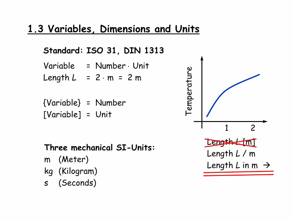
1.3 Variables, Dimensions and Units
Standard: ISO 31, DIN 1313
Variable = Number Unit
Length L = 2 m = 2 m
{Variable} = Number
[Variable] = Unit
Three mechanical SI-Units:
m (Meter)
kg (Kilogram)
s (Seconds)
Length L [m]
Length L / m
Length L in m
21
Tem
pera
ture
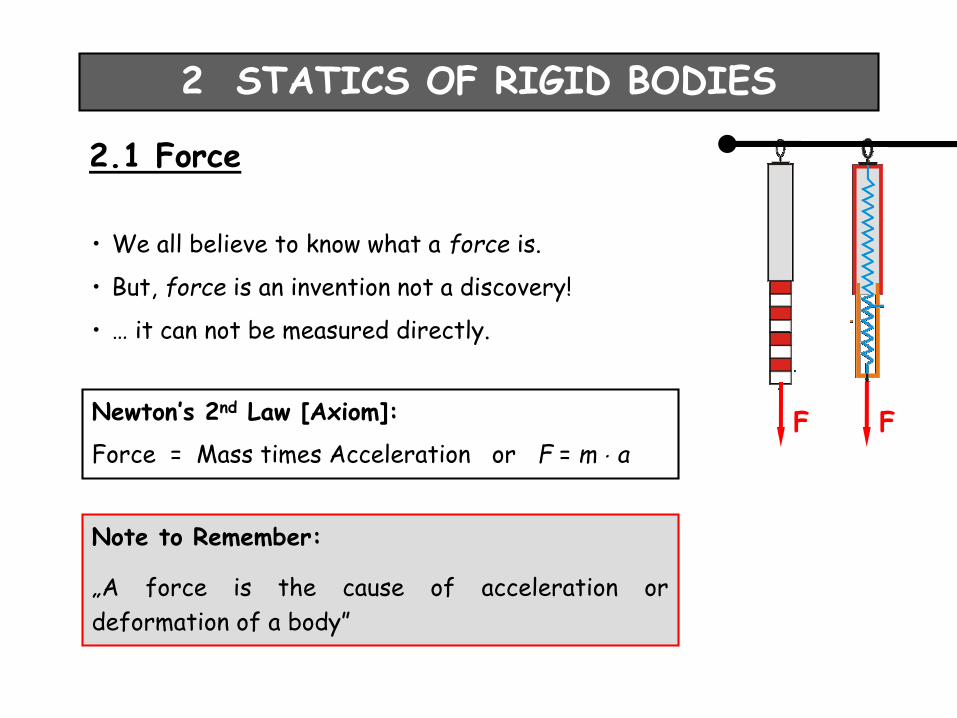
Note to Remember:
„A force is the cause of acceleration or
deformation of a body”
Newton’s 2nd Law [Axiom]:
Force = Mass times Acceleration or F = m a
• We all believe to know what a force is.
• But, force is an invention not a discovery!
• … it can not be measured directly.
2.1 Force
2 STATICS OF RIGID BODIES
F F

... with arrows
Forces are Vectors with
Magnitude
Direction
Sense of Direction
Representation of Forces
5 N
Line of action
Screw

Units of Force
Newton
N = kgm/s2
1 N
Note to Remember:
1 Newton Weight of a bar of chocolate (100 g)
FG = mg = 0,1 kg 9,81 m/s2
= 0,981 kg m/s2
1 N
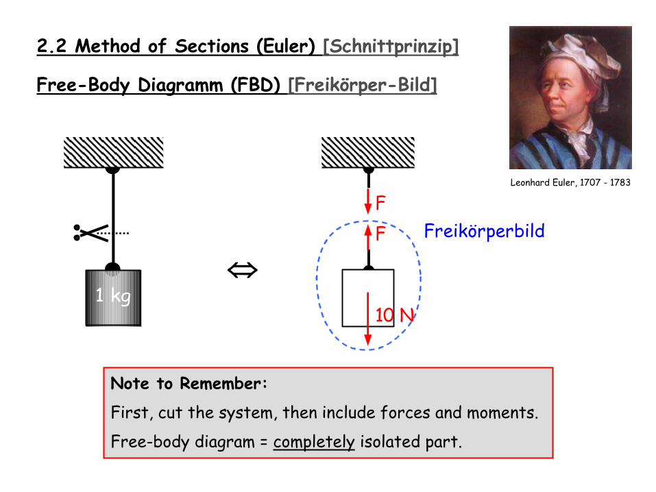
2.2 Method of Sections (Euler) [Schnittprinzip]
Note to Remember:
First, cut the system, then include forces and moments.
Free-body diagram = completely isolated part.
Free-Body Diagramm (FBD) [Freikörper-Bild]
Leonhard Euler, 1707 - 1783
1 kg
F
F
Freikörperbild
10 N
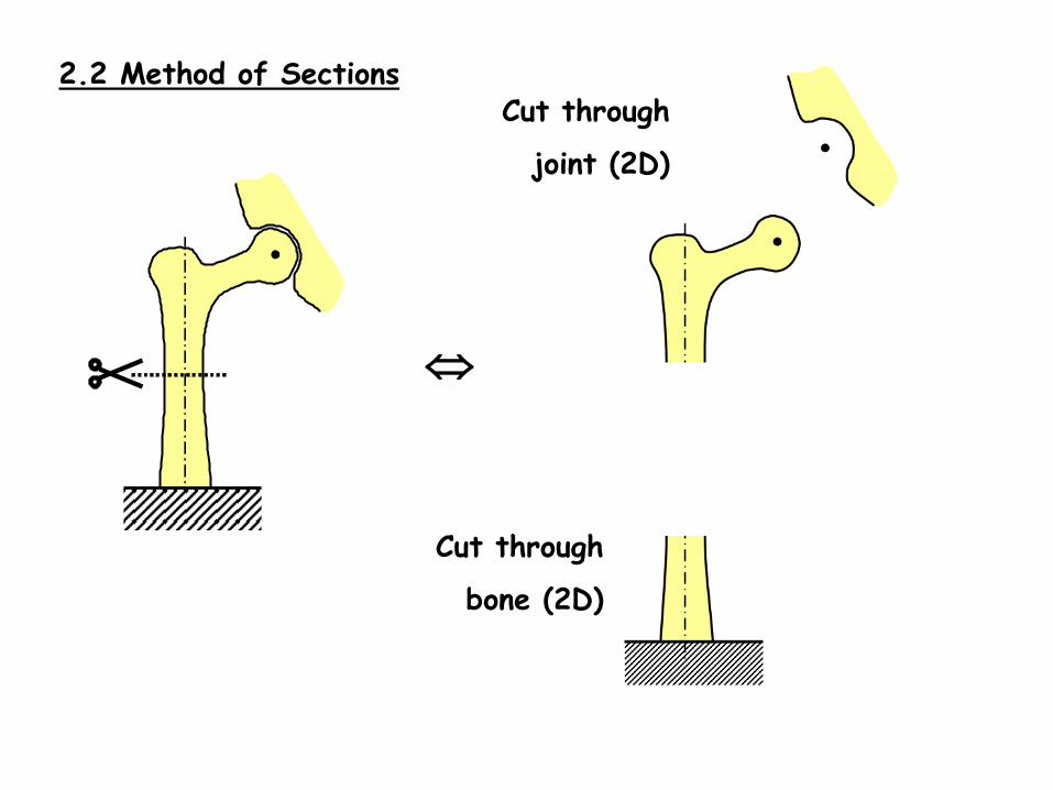
Cut through
bone (2D)
Cut through
joint (2D)
2.2 Method of Sections
Cut through
bone (2D)
Cut through
joint (2D)
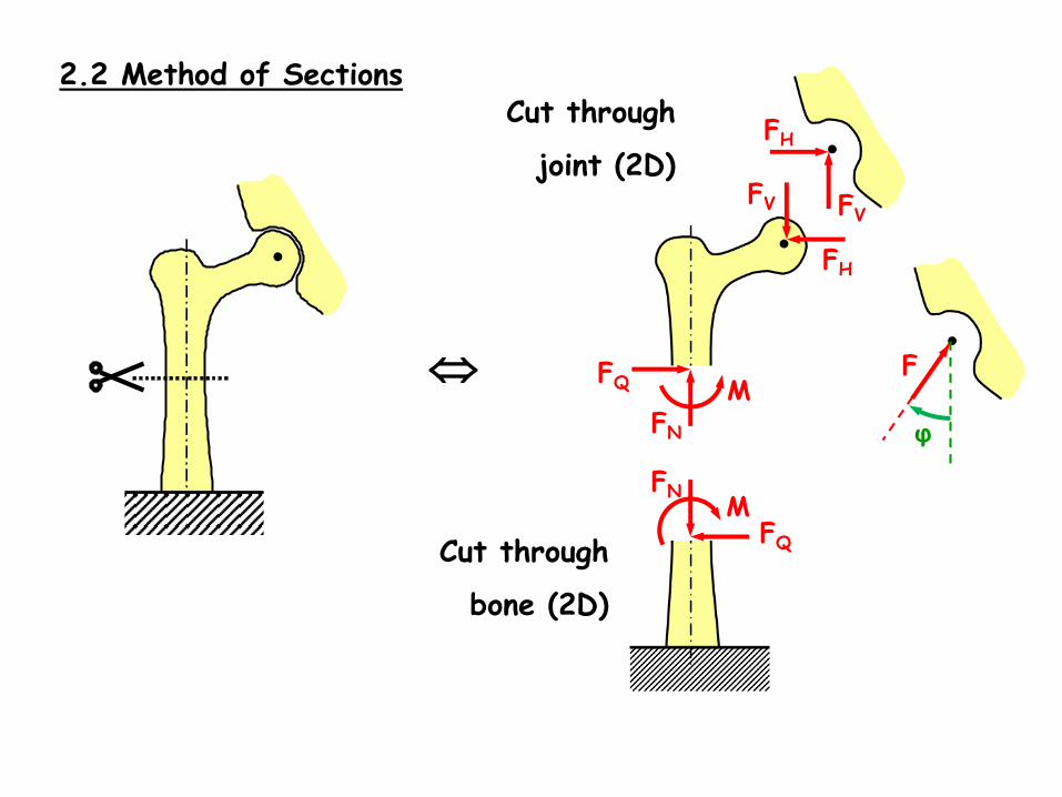
2.2 Method of Sections
FN
FN
FQ
FQ
M
M
FH
FVFV
FH
F
φ
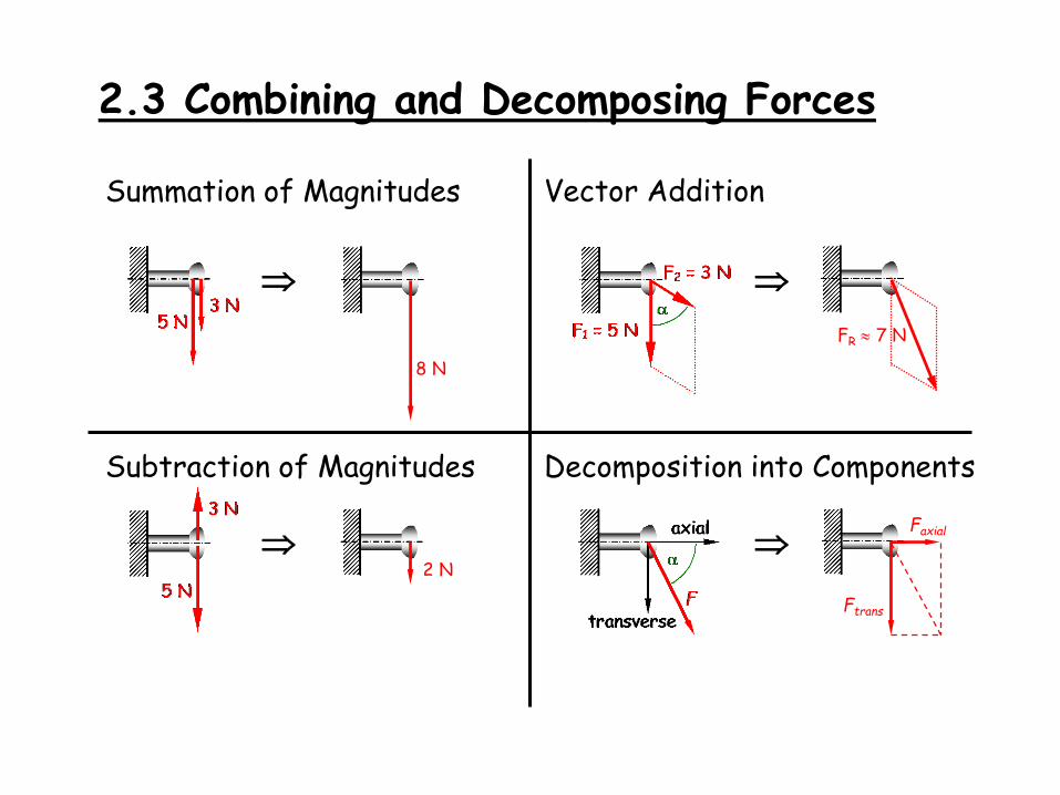
2.3 Combining and Decomposing Forces
Summation of Magnitudes
Subtraction of Magnitudes Decomposition into Components
Vector Addition
8 N
2 N
FR 7 N
Ftrans
Faxial

2.4 The Moment [Das Moment]
Note to remember:
The moment M = F a is equivalent to a force couple (F, a).
A moment is the cause for angular acceleration or angular de-formation (Torsion, Bending) of a body.
Screw Blade
Slotted screw with
screwdriver blade M = Fa
Force Couples (F, a) Moment M
F
F a
F
F
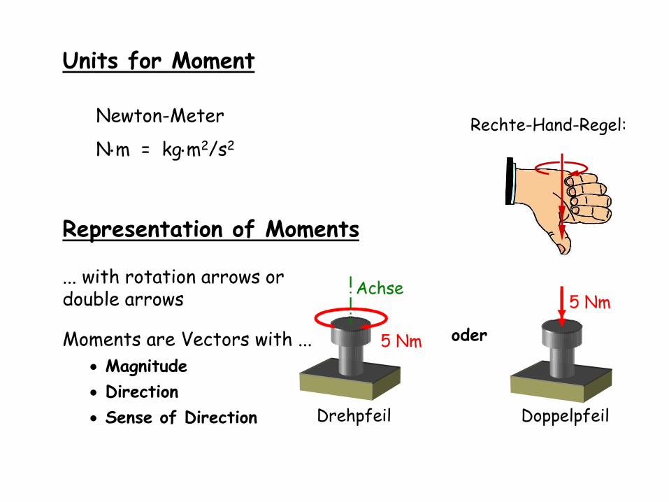
Units for Moment
Newton-Meter
Nm = kgm2/s2
Representation of Moments
... with rotation arrows or double arrows
Moments are Vectors with ...
Magnitude
Direction
Sense of Direction
Rechte-Hand-Regel:
5 Nm
Achse
Drehpfeil
5 Nm
Doppelpfeil
oder
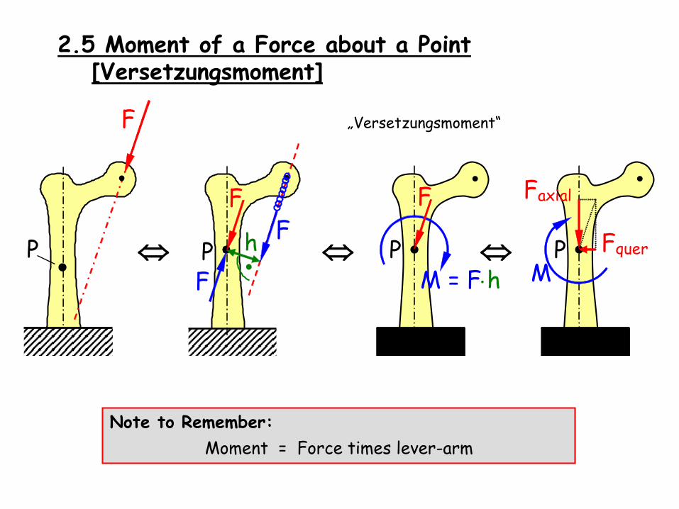
2.5 Moment of a Force about a Point [Versetzungsmoment]
Note to Remember:
Moment = Force times lever-arm
F
P
P M = Fh
F
F
h P
P M
Faxial
Fquer
F
F
„Versetzungsmoment“

2.7 Static Equilibrium
Important:
Free-body diagram (FBD) first, then equilibrium!
For 2D Problems max. 3 equations for each FBD:
(For 3D Problems max. 6 equations for each FBD)
F
F
10 N
Free-body diagram
(FBD)
The sum of all forces in x-direction equals zero:
The sum of all forces in y-direction equals zero:
The sum of Moments with respect to P equals zero:
0...!
,2,1 yy FF
0...!
,2,1 P
z
P
z MM
0...!
,2,1 xx FF

.0...:P toresp. w.moments all of Sum
,0...:direction-yin forces all of Sum
,0...:direction-in x forces all of Sum
!
,2,1
!
,2,1
!
,2,1
P
z
P
z
yy
xx
MM
FF
FF
Force EEs can be substituted by moment EEs
3 moment reference points should not lie on one line
3 equations of equilibrium for each FBD in 2D:
2.7 Static Equilibrium
Important:
Free-body diagram (FBD) first, then equilibrium!
F
F
10 N
Free-body diagram
(FBD)
.0 :RPunkt bezüglich Achse-z um Momentealler Summe
.0 :QPunkt bezüglich Achse-y um Momentealler Summe
.0 :PPunkt bezüglich Achse- xum Momentealler Summe
,0 :Richtung-zin Kräftealler Summe
,0 :Richtung-yin Kräftealler Summe
,0 :Richtung-in x Kräftealler Summe
!
!
!
!
!
!
i
R
iz
i
Q
iy
i
P
ix
i
iz
i
iy
i
ix
M
M
M
F
F
F
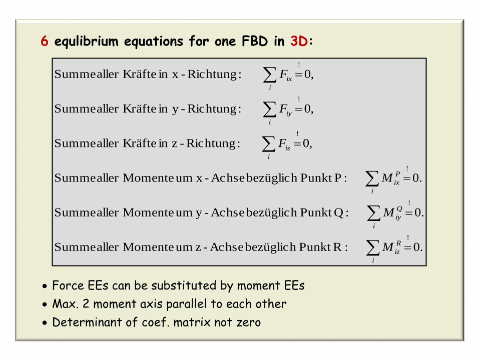
6 equlibrium equations for one FBD in 3D:
Force EEs can be substituted by moment EEs
Max. 2 moment axis parallel to each other
Determinant of coef. matrix not zero
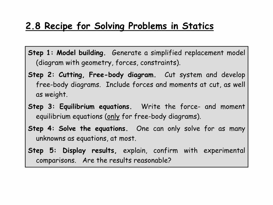
2.8 Recipe for Solving Problems in Statics
Step 1: Model building. Generate a simplified replacement model
(diagram with geometry, forces, constraints).
Step 2: Cutting, Free-body diagram. Cut system and develop
free-body diagrams. Include forces and moments at cut, as well
as weight.
Step 3: Equilibrium equations. Write the force- and moment
equilibrium equations (only for free-body diagrams).
Step 4: Solve the equations. One can only solve for as many
unknowns as equations, at most.
Step 5: Display results, explain, confirm with experimental
comparisons. Are the results reasonable?

2.9 Classical Example: „Biceps Force“
From: „De Motu Animalium“G.A. BORELLI (1608-1679)

Step 1: Model building
Rope (fixed length)
10 kg
Beam
(rigid, massless)
Joint
(frictionless)
Rigid
fixation
g

10 kg
1
2
3
Schritt 2: Schneiden und Freikörperbilder
S1
S1
S2
S2
S3
S3
100 N
A
B
C
4

S2
S3
B
More to Step 2: Cutting and Free-Body Diagrams
Step 3 and 4: Equilibrium and Solving the Equations
Sum of all forces in vertical direction = 0
Sum of all forces in “rope” direction = 0
S1 = 100 N
S2
h2
h1 G
C
Sum of all moments with respect to Point G = 0
S1
100 N
A
N100
0)(N100
1
!
1
S
S
23
!
32 0)(
SS
SS
N700cm5
cm35 N100
0cm5cm35N100
0
2
!
2
!
2211
S
S
hShS
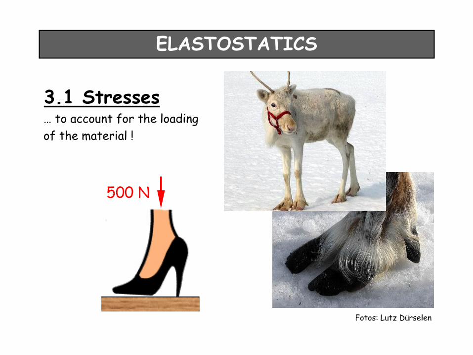
ELASTOSTATICS
500 N
… to account for the loading
of the material !
Fotos: Lutz Dürselen
3.1 Stresses

Note to Remember:
Stress = „smeared“ force
Stress = Force per Area or = F/A
(Analogy: „Nutella bread teast “)
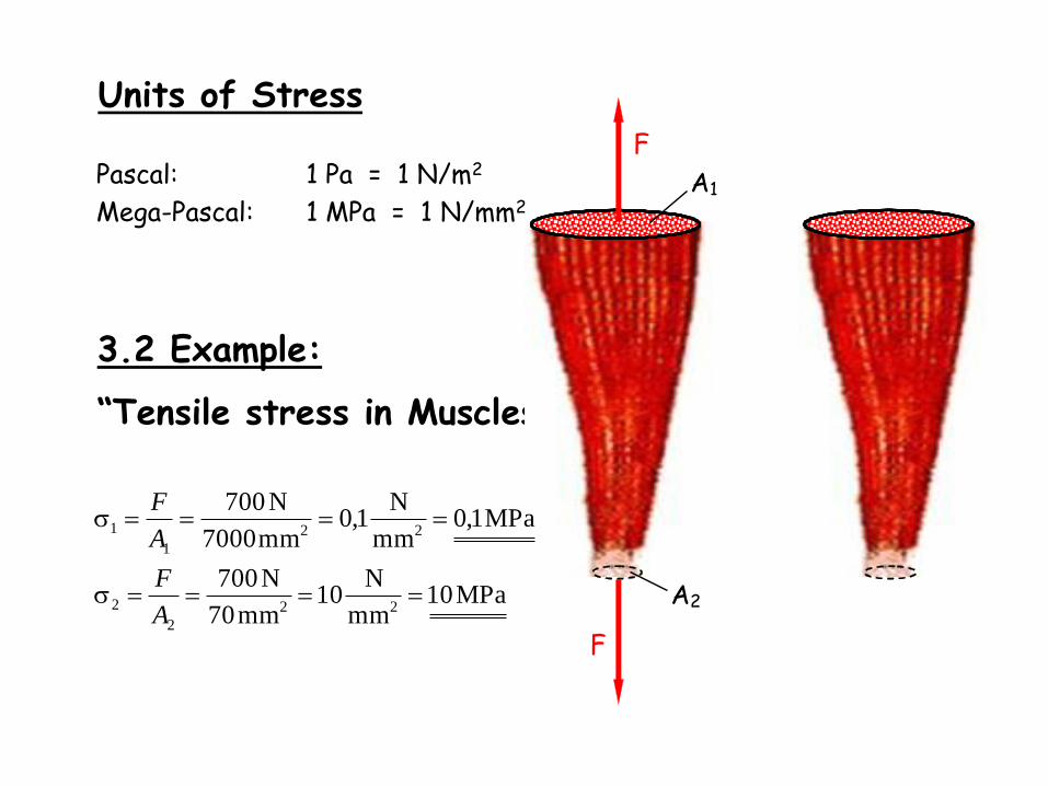
Units of Stress
3.2 Example:
“Tensile stress in Muscles”
Pascal: 1 Pa = 1 N/m2
Mega-Pascal: 1 MPa = 1 N/mm2
F
F
A1
A2 MPa10mm
N10
mm70
N700
MPa1,0mm
N1,0
mm7000
N700
22
2
2
22
1
1
A
F
A
F

F
P
1
P
Cut 1:Normal stress 1
Cut 2:Normal stress 2
Shear stress 2
Tensile bar
1
2
3.3 Normal and Shear Stresses
Note to Remember:
First, you must choose a point and a cut through the point,
then you can specify (type of) stresses at this point in the
body.
Normal stresses (tensile and compressive stress) are
oriented perpendicular to the cut-surface.
Shear stresses lie tangential to the cut-surface.
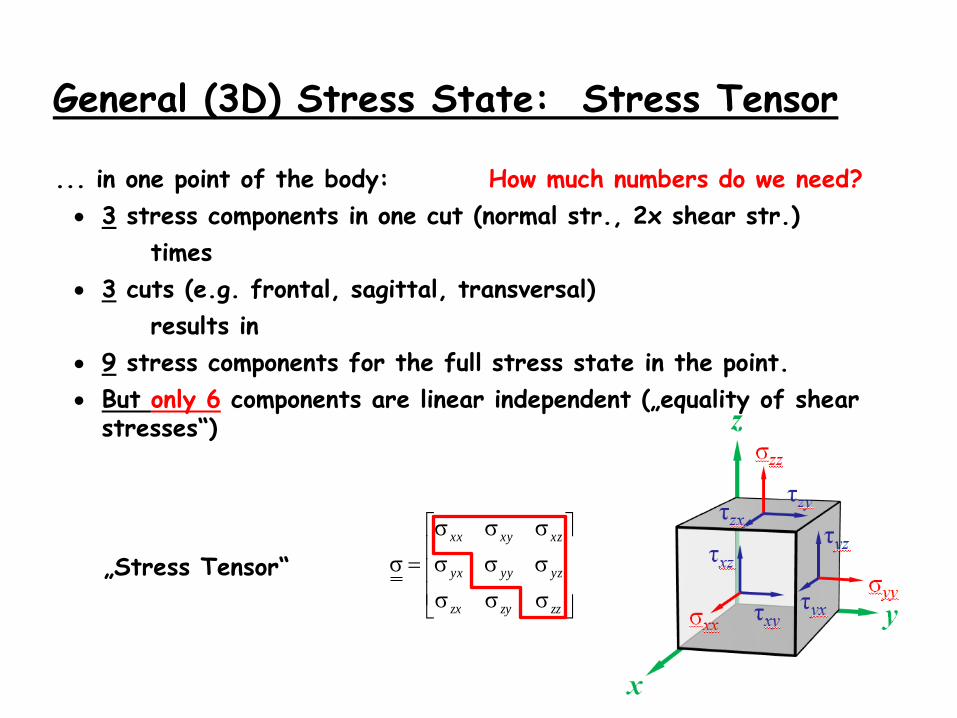
General (3D) Stress State: Stress Tensor
... in one point of the body: How much numbers do we need?
3 stress components in one cut (normal str., 2x shear str.)
times
3 cuts (e.g. frontal, sagittal, transversal)
results in
9 stress components for the full stress state in the point.
But only 6 components are linear independent („equality of shearstresses“)
zzzyzx
yzyyyx
xzxyxx
„Stress Tensor“

Symmetry of the Stress Tensor
Boltzmann Continua: Only volume forces (fx und fy), no volume moments assumed
„Equality of corresponding shear stresses“
zz
yzyy
xzxyxx
.sym
.y
σyy
x
fy
C
τyx
τyx
τxy
τxy
σxxσxx fx
σyy

6 Components 6 Pictures
General 3D Stress State

Problem:
How to produce nice Pictures?
Which component should I use?
Do I need 6 pictures at the same time?
So called „Invariants“ are „smart mixtures“ of the components
Mises xx2 yy
2 zz2 xx yy xx zz yy zz 3 xy
2 3 xz2 3 yz
2

3.4 Strains
• Global, (external) strains
• Local, (internal) strains
Distortional Strain in a fracture callus
Units of Strain
without a unit
1
1/100 = %
1/1.000.000 = με (micro strain)
= 0,1 %
Gap
0lengthOriginal
lengthinChange:
L
L
Finite element model of the fracture callus

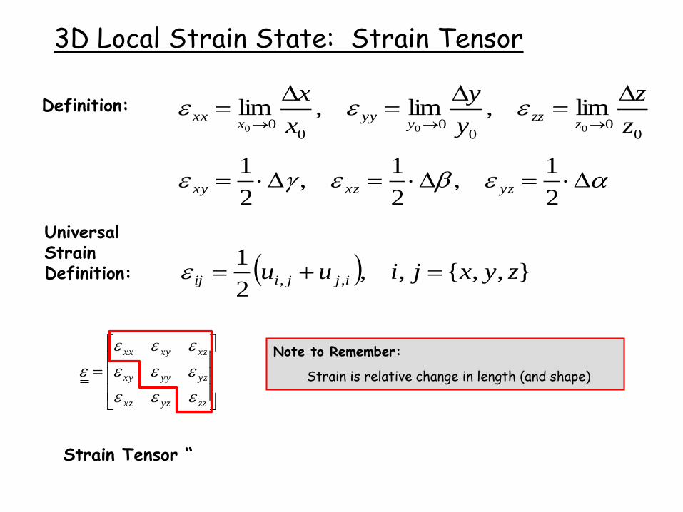
3D Local Strain State: Strain Tensor
undeformed deformed
y+δy
xy +δxy
x+δx
y
xy
xz
Displacements[Verschiebungen]
zzyzxz
yzyyxy
xzxyxx
Strain Tensor “
00
00
00 000
lim,lim,limz
z
y
y
x
x
zzz
yyy
xxx
2
1,
2
1,
2
1yzxzxy
Definition:
},,{,,2
1,, zyxjiuu ijjiij
Universal Strain Definition:
3D Local Strain State: Strain Tensor
Note to Remember:
Strain is relative change in length (and shape)
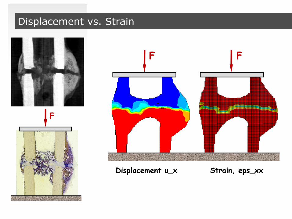
Displacement vs. Strain
Displacement u_x Strain, eps_xx
F F
F

Anisotropic Properties
Material
E Moduli
in MPa
Strength
in MPa
Fracture
strain
in %
Spongy bone
Vertebra 60 (male)
35 (female)
4,6 (male)
2,7 (female)
6
prox. Femur 240 2.7 2.8
Tibia 450 5...10 2
Bovine 200...2000 10 1,7...3,8
Ovine 400...1500 15
Cortical bone
Longitudinal 17000 200 2,5
Transversal 11500 130
Top Related