


Languages
Pages
Legal

11/13/18
1
ECE241–AdvancedProgrammingIFall2018MikeZink
Lecture17DivideandConquer–
FastFourierTransform(FFT)
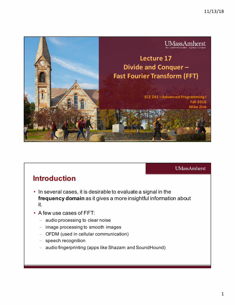
Introduction• In several cases, it is desirable to evaluate a signal in the
frequency domain as it gives a more insightful information about it.
• A few use cases of FFT:– audio processing to clear noise– image processing to smooth images– OFDM (used in cellular communication)– speech recognition– audio fingerprinting (apps like Shazam and SoundHound)

11/13/18
2
• Given the original signal, 𝑓(𝑡), the Fourier transform is denoted by
𝐹 𝑗𝜔 = ) 𝑓(𝑡)𝑒+,-./𝑑𝑡1
+1
• It decomposes the signal in the time domain into the frequency domain. For example:
2
Fourier Transform
Piano note, E4. (Source: Time-Frequency Analysis of Musical Instruments)
• The square wave on the top left is composed of a sum of multiple sine waves.
• Fourier Transform allows us to visualize a signal in the frequency domain, showing all its components, called harmonics.
• The Fourier Transform is also useful to find distortions in a signal (among other applications).
3
Fourier Transform
11/13/18
3
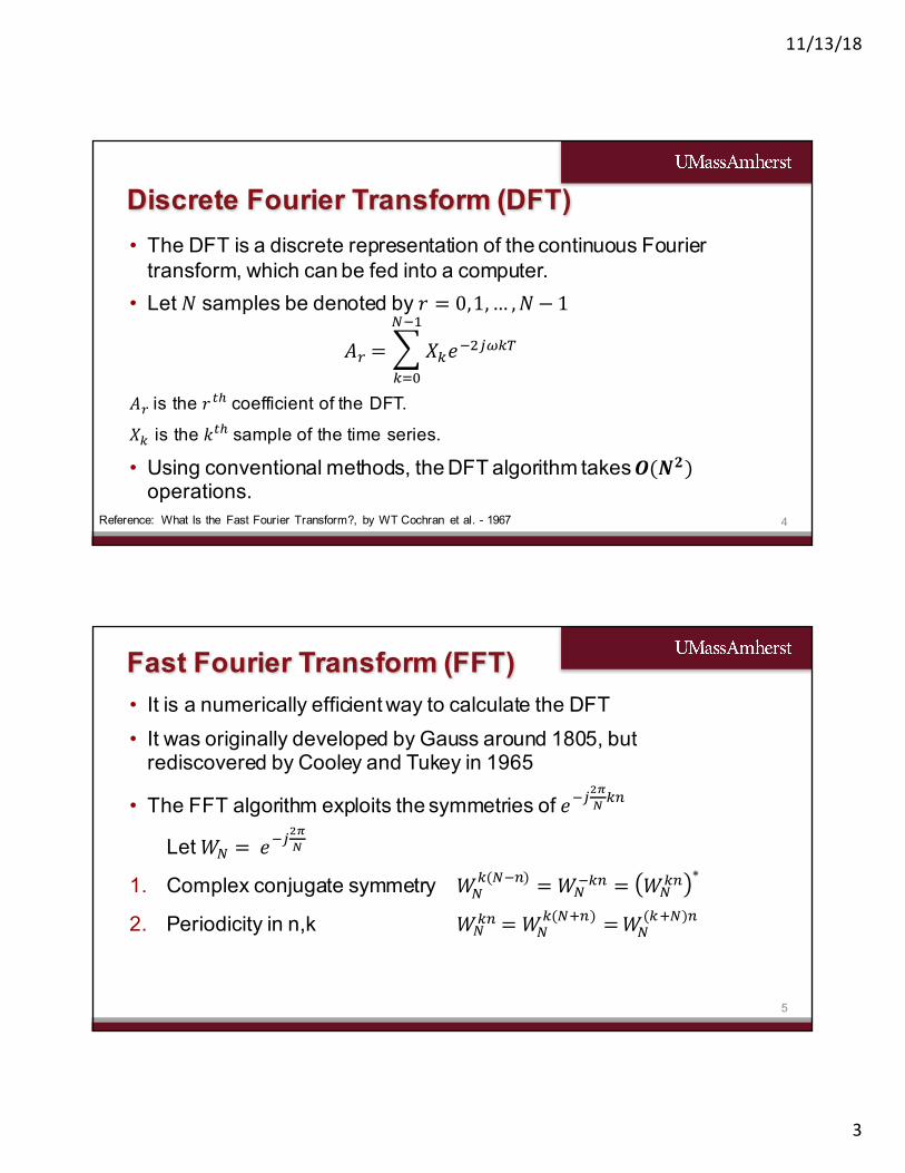
• The DFT is a discrete representation of the continuous Fourier transform, which can be fed into a computer.
• Let 𝑁 samples be denoted by 𝑟 = 0,1,… ,𝑁 − 1
𝐴: = ; 𝑋=𝑒+,-.=>?+@
=AB
𝐴: is the 𝑟/C coefficient of the DFT.
𝑋= is the 𝑘/C sample of the time series.
• Using conventional methods, the DFT algorithm takes 𝑶(𝑵𝟐)operations.
4
Discrete Fourier Transform (DFT)
Reference: What Is the Fast Fourier Transform?, by WT Cochran et al. - 1967
• It is a numerically efficient way to calculate the DFT• It was originally developed by Gauss around 1805, but
rediscovered by Cooley and Tukey in 1965
• The FFT algorithm exploits the symmetries of 𝑒+-HIJ =K
Let 𝑊? =𝑒+-HIJ
1. Complex conjugate symmetry 𝑊?=(?+K) = 𝑊?
+=K = 𝑊?=K ∗
2. Periodicity in n,k 𝑊?=K = 𝑊?
=(?OK) =𝑊?(=O?)K
5
Fast Fourier Transform (FFT)
11/13/18
4
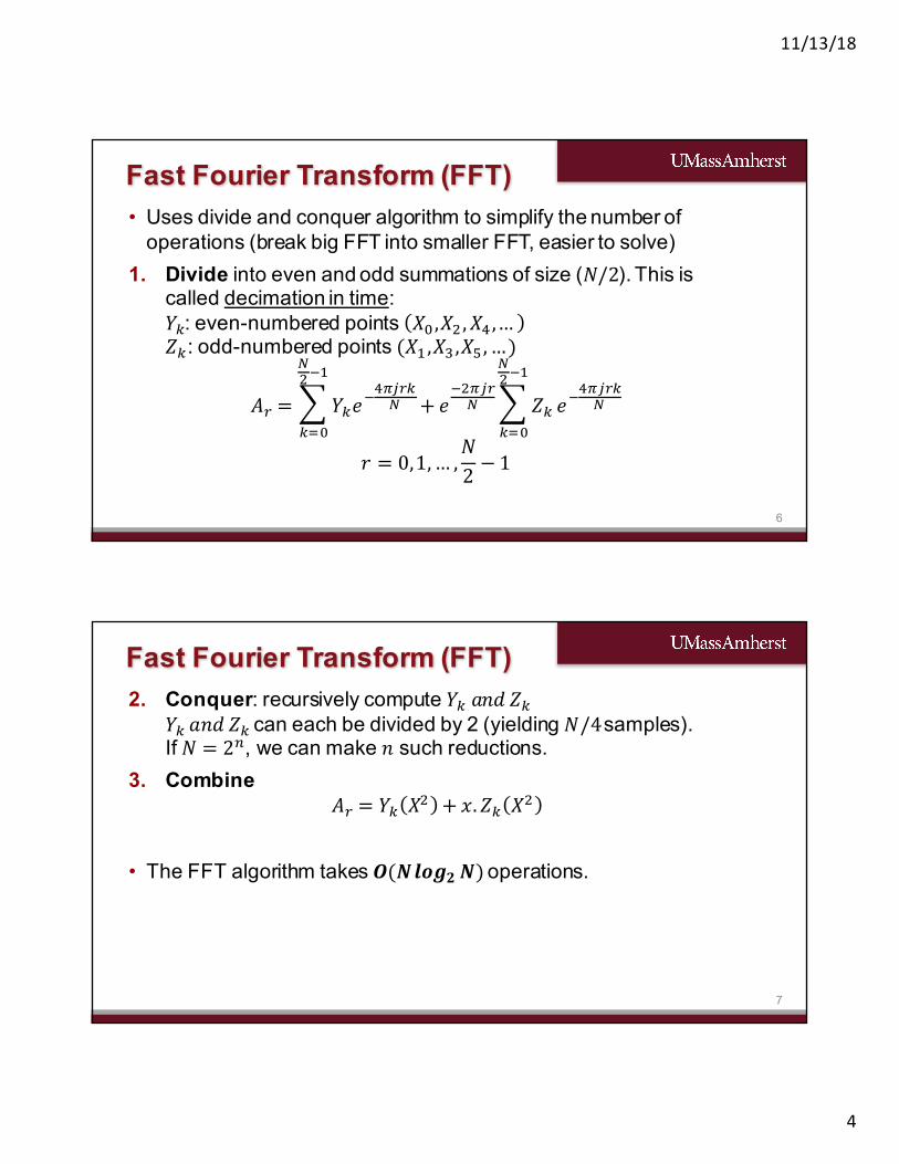
• Uses divide and conquer algorithm to simplify the number of operations (break big FFT into smaller FFT, easier to solve)
1. Divide into even and odd summations of size (𝑁/2). This is called decimation in time:𝑌=: even-numbered points 𝑋B,𝑋,, 𝑋S,…𝑍=: odd-numbered points (𝑋@,𝑋U,𝑋V,…)
𝐴: = ; 𝑌=𝑒+SW-:=?
?,+@
=AB
+ 𝑒+,W-:? ; 𝑍=
?,+@
=AB
𝑒+SW-:=?
𝑟 = 0,1,… ,𝑁2 − 1
6
Fast Fourier Transform (FFT)
2. Conquer: recursively compute𝑌=𝑎𝑛𝑑𝑍=𝑌=𝑎𝑛𝑑𝑍=can each be divided by 2 (yielding 𝑁/4samples). If 𝑁 = 2K, we can make 𝑛 such reductions.
3. Combine𝐴: = 𝑌= 𝑋, + 𝑥. 𝑍= 𝑋,
• The FFT algorithm takes 𝑶(𝑵𝒍𝒐𝒈𝟐 𝑵)operations.
7
Fast Fourier Transform (FFT)

11/13/18
5
8
Example for N=8
Even indexed
terms
Odd indexed
terms
𝑁2
,∗ 2 +𝑁 ≈ ?
,
,+ N
• Keep splitting the terms, i.e., each ?,
= 2 ∗ ?S
DFTs
• We can split log,𝑁 times• As N gets large
≈ 𝑂(𝑁log,𝑁)
9
Example for N=8

11/13/18
6
10
DFT algorithm implementation in Pythonimport numpy as npfrom timeit import Timer
pi2 = np.pi * 2
def DFT(x):N = len(x) FmList = [] for m in range(N):
Fm = 0.0 for n in range(N):
Fm += x[n] * np.exp(- 1j * pi2 * m * n / N) FmList.append(Fm / N)
return FmList
N = 1000x = np.arange(N)t = Timer(lambda: DFT(x))print('Elapsed time: {} s'.format(str(t.timeit(number=1))))
11
DFT Performance
0.10 0.69
605.29
2650.96
0.00
500.00
1000.00
1500.00
2000.00
2500.00
3000.00
128 1024 32768 65536
Tim
e (s
econ
ds)
Number of Samples
DFT Computation Time
DFT
All this and following experiments were run on a virtual machine running Ubuntu 18.04 LTS with one processor (Intel(R) Core(TM) i5-4300U CPU @ 1.90GHz) and 3GB of memory.

11/13/18
7
12
FFT algorithm implementation in Python
13
FFT algorithm implementation in Python# Recursive FFT function
import numpy as np
def FFT(x): N = len(x)
if N <= 1: return x even = FFT(x[0::2]) odd = FFT(x[1::2]) T = [np.exp(-2j * np.pi * k / N) * odd[k] for k in range(N // 2)] return [even[k] + T[k] for k in range(N // 2)] + \ [even[k] - T[k] for k in range(N // 2)] N = 1024x = np.random.random(N)t = Timer(lambda: FFT(x))print('Elapsed time: {} s'.format(str(t.timeit(number=1))))

11/13/18
8
14
FFT Performance
0.08 0.100.40
0.890.10
0.69
605.292650.96
0.01
0.10
1.00
10.00
100.00
1000.00
10000.00
128 1024 32768 65536
Tim
e (s
econ
ds)
Number of Samples
DFT vs. FFT
FFT
DFT
Log Scale
15
Numpy implementations# FFT example using the Numpy fftpack
import numpy as npfrom timeit import Timer
N = 10000x = np.arange(N)t = Timer(lambda: np.fft.fft(x))print('Elapsed time: {} s'.format(str(t.timeit(number=1))))
11/13/18
9
16
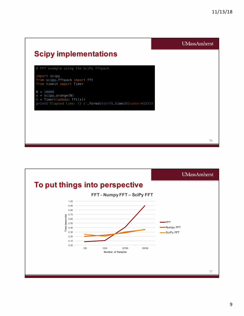
Scipy implementations# FFT example using the SciPy fftpack
import scipyfrom scipy.fftpack import fftfrom timeit import Timer
N = 10000x = scipy.arange(N)t = Timer(lambda: fft(x))print('Elapsed time: {} s'.format(str(t.timeit(number=1))))
17
To put things into perspective
0.00
0.10
0.20
0.30
0.40
0.50
0.60
0.70
0.80
0.90
1.00
128 1024 32768 65536
Tim
e (s
econ
ds)
Number of Samples
FFT - Numpy FFT – SciPy FFT
FFT
Numpy FFT
SciPy FFT

11/13/18
10
• Audio fingerprinting is a signature that summarizes an audio recording
• Also known as Content-Based audio Identification (CBID)• The best known application are apps like Shazam and
SoundHound, that link unlabeled audio recordings to a corresponding metadata (song name and artist, for instance)
18
Application – Audio Fingerprinting
Source: http://willdrevo.com/fingerprinting-and-audio-recognition-with-python/ for all following slides, unless otherwise stated
• Sampling: the standard sampling rate in digital music, such as HIFI, is 44,100 samples per second (from Nyquist theorem – 2 x 20 kHz)
• Quantization: the standard quantization uses 16 bits, or 65,536 levels
• PCM or Pulse Code Modulation: is the representation of the analog signal into zeros and ones
• This means that each second of music will have 44,100 samples per channel (one channel – Mono; two channels – Stereo)E.g.: 3 minutes of stereo song will have 15,876,000 samples
19
Background on Digital Audio
11/13/18
11
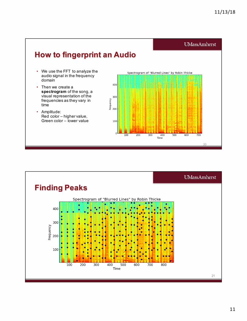
• We use the FFT to analyze the audio signal in the frequency domain
• Then we create a spectrogram of the song, a visual representation of the frequencies as they vary in time
• Amplitude:Red color – higher value, Green color – lower value
20
How to fingerprint an Audio
21
Finding Peaks

11/13/18
12
22
Fingerprint Hashing
• We hash the frequency of peaks and the time difference between them
• The result is a unique fingerprint for the song
• Each app has its own hashing function to uniquely identify a song
23
How Shazam Works in a Nutshell
Source: An Industrial-Strength Audio Search Algorithm, by Avery Li-Chun Wang (Shazam Whitepaper)
Speaker
AmbientNoise
MIC
1. Receive audio and
noise2. Fingerprinting
3. Send to Shazam
Shazam DB
4. Compare with current fingerprinting database
5. Send Title and artist
11/13/18
13
Top Related