


Languages
Pages
Legal

Deep ReinforcementLearning in TensorFlowDanijar Hafner · Stanford CS 20SI · 2017-03-10

Repeat until end of episode:
Most methods also work with partial observation instead of stateNo perfect example output as in supervised learning
Reinforcement Learning
5
Agent Environment
1. State
2. Action
3. Reward
+5

Formalization as Markov Decision ProcessEnvironment:
Markovian states s ϵ S and actions a ϵ AScalar reward function R(rt | st, at)Transition function P(st+1 | st, at)
Agent:Act according to stochastic policy π(at | s0 , …, st)Collects experience tuples (st, at, rt, st+1)
Objective:Maximize expectation of return Rt = ∑i=0, …, ∞ γi rt+i discounted by 0 < γ < 1
6

Overview of Methods
7
Model BasedPolicy BasedValue Based Actor Critic
DQN
NFQ
DDQN
A3C
DPG
DDPGNAF
TRPO
GAE
REINFORCE
Planning
MPC
AlphaGo
Value Based Methods

Value Learning
9
Value function V(st) = E[ Rt ] = E[ ∑i=0, …, ∞ γi rt+i ]
Bellman equation V(s) = r + γ∑s'ϵS{ P(s'|s, π(a|s))V(s') }
Act according to best V(s'), sometimes randomly
Estimate V(s) using learning rate
V'(s) = (1 - α) V(s) + α (r + V(s'))
Converges to true value function and optimal behavior
Problem: Need P(s'|s) to act (as in board games, for example Go)
Andy Zeng (http://www.cs.princeton.edu/~andyz/pacmanRL)

Q Learning (Watkins89)Learn Q function Q(st, at) = E[ Rt ] instead
Bellman equation Q*(s, a) = r + γ maxa'ϵAQ*(s', a')
Act according to best Q(s, a), sometimes randomly
Estimate Q*(s, a) using learning rate
Q'(s, a) = (1 - α) Q(s, a) + α (r + maxa'ϵAQ(s', a'))
Converges to optimal function Q*(s, a) and optimal behavior
Doesn't depend on policy, can learn from demonstrations or old experience10
Andy Zeng (http://www.cs.princeton.edu/~andyz/pacmanRL)

Comparison Value Learning and Q-Learning
11
π(s) = argmaxaϵA Q(s, a)π(s) = argmaxaϵA { ∑s'ϵS P(s'|s, a) V(s') }

Epsilon Greedy ExplorationConvergence and optimality only when visiting each state infinitely often
Exploration is a main challenge in reinforcement learning
Simple approach is acting randomly with probability ε
Will visit each (s, a) infinitely often in the limit
Decay ε exponentially to ensure converge
Right amount of exploration is often critical in practice
12

epsilon = exponential_decay(step, 50000, 1.0, 0.05, rate=0.5)best_action = tf.arg_max(_qvalues([observ])[0], 0)random_action = tf.random_uniform((), 0, num_actions, tf.int64)should_explore = tf.random_uniform((), 0, 1) < epsilonreturn tf.cond(should_explore, lambda: random_action, lambda: best_action)
def exponential_decay(step, total, initial, final, rate=1e-4, stairs=None): if stairs is not None: step = stairs * tf.floor(step / stairs) scale, offset = 1. / (1. - rate), 1. - (1. / (1. - rate)) progress = tf.cast(step, tf.float32) / tf.cast(total, tf.float32) value = (initial - final) * scale * rate ** progress + offset + final lower, upper = tf.minimum(initial, final), tf.maximum(initial, final) return tf.maximum(lower, tf.minimum(value, upper))

Deep Neural Networks

Nonlinear Function ApproximationToo many states for a lookup table
We want to approximate Q(s, a) using a deep neural network
Can capture complex dependencies between s, a and Q(s, a)
Agent can learn sophisticated behavior!
Convolutional networks for reinforcement learning from pixels
Share some tricks from papers of the last two years
Sketch out implementations in TensorFlow15
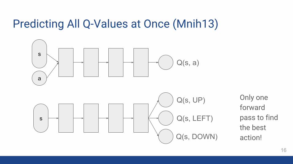
Predicting All Q-Values at Once (Mnih13)
16
s
Q(s, UP)
Q(s, DOWN)
Q(s, LEFT)
a
sQ(s, a)
Only one forward pass to find the best action!

def _qvalues(observ): with tf.variable_scope('qvalues', reuse=True): # Network from DQN (Mnih 2015) h1 = tf.layers.conv2d(observ, 32, 8, 4, tf.nn.relu) h2 = tf.layers.conv2d(h1, 64, 4, 2, tf.nn.relu) h3 = tf.layers.conv2d(h2, 64, 3, 1, tf.nn.relu) h4 = tf.layers.dense(h3, 512, tf.nn.relu) return tf.layers.dense(h4, num_actions, None)
current = tf.gather(_qvalues(observ), action)[:, 0]target = reward + gamma * tf.reduce_max(_qvalues(nextob), 1)target = tf.where(done, tf.zeros_like(target), target)loss = (current - target) ** 2

Trick 1: Experience Replay (Mnih13)Stochastic gradient descent expects independent samples
Agent collects highly correlated experience at a time
Store experience tuples in a large buffer and select random batch for training
Decorrelates training examples!
Even better: Select training examples prioritized by last training cost (Schaul15)
Focuses on rare training examples!
18

def sample(self, amount): positions = tf.random_uniform( (amount,), 0, self.size - 1, tf.int32) return [tf.gather(b, positions) for b in self._buffers]
def _create_buffers(self, template): buffers = [] for tensor in template: shape = tf.TensorShape( [self._capacity]).concatenate( tensor.get_shape()) initial = tf.zeros(shape, tensor.dtype) buffers.append(tf.Variable( initial, trainable=False)) return buffers
class ReplayBuffer:
def __init__(self, template, capacity): self._capacity = capacity self._buffers = self._create_buffers( template) self._index = tf.Variable( 0, dtype=tf.int32, trainable=False)
def size(self): return tf.minimum( self._index, self._capacity)
def append(self, tensors): position = tf.mod( self._index, self._capacity) with tf.control_dependencies([ b[position].assign(t) for b, t in zip(self._buffers, tensors)]): return self._index.assign_add(1)

class PrioritizedReplayBuffer:
def __init__(self, template, capacity): template = (tf.constant(0.0),) + tuple(template) self._buffer = ReplayBuffer(template, capacity)
def size(self): return self._buffer.size
def append(self, priority, tensors): return self._buffer.append((priority,) + tuple(tensors))
def sample(self, amount, temperature=1): priorities = self._buffer._buffers[0].value()[:self._buffer.size()] logprobs = tf.log(priorities / tf.reduce_sum(priorities)) / temperature positions = tf.multinomial(logprobs[None, ...], amount)[0] return [tf.gather(b, positions) for b in self._buffer._buffers[1:]]

Trick 2: Target Network (Mnih15, Lillicrap16, ...)Targets r + γ maxa'ϵAQ(s', a') depend on own current network Q(s, a)
Training towards moving target makes training unstable
Use a moving average QT(s, a) of the network to compute the targets
Update network parameters θTt+1 = (1 - β) θT
t + β θt with β << 1
Get weights using graph editor and apply tf.train.ExponentialMovingAverage
Use graph editor to copy network graph and bind to averaged variables
21

def bind(output, inputs): for key in inputs: if isinstance(inputs[key], tf.Variable): inputs[key] = inputs[key].value() return tf.contrib.graph_editor.graph_replace(output, inputs)
def moving_average( output, decay=0.999, collection=tf.GraphKeys.TRAINABLE_VARIABLES): average = tf.train.ExponentialMovingAverage(decay=decay) variables = set(v.value() for v in output.graph.get_collection(collection)) deps = tf.contrib.graph_editor.get_backward_walk_ops(output) deps = [t for o in deps for t in o.values()] deps = set([t for t in deps if t in variables]) update_op = average.apply(deps) new_output = bind(output, {t: average.average(t) for t in deps}) return new_output, update_op
current = tf.gather(_qvalues(observ), action)[:, 0]target_qvalues = moving_average(_qvalues(nextob), 0.999)target = reward + gamma * tf.reduce_max(target_qvalues, 1)target = tf.where(done, tf.zeros_like(target), target)loss = (current - target) ** 2

Trick 3: Double Q Learning (Hasselt10, Hasselt15)Q Learning tends to overestimate Q values
Same network chooses best action and evaluates it
r + γ maxa'ϵAQ(s', a') = r + γ Q(s', argmaxa'ϵAQ(s', a'))
Learning two Q functions from different experience would be ideal
For efficiency, use target network QT(s, a) to evaluate action
Targets become r + γ QT(s', argmaxa'ϵAQ(s', a'))
23

# Q Learningcurrent = tf.gather(_qvalues(observ), action)[:, 0]target_qvalues = moving_average(_qvalues(nextob), 0.999)target = reward + gamma * tf.reduce_max(target_qvalues, 1)target = tf.where(done, tf.zeros_like(target), target)loss = (current - target) ** 2
# Double Q Learningcurrent = tf.gather(_qvalues(observ), action)[:, 0]target_qvalues = moving_average(_qvalues(nextob), 0.999)future_action = tf.argmax(_qvalues(nextob), 1)target = reward + gamma * tf.gather(target_qvalues, future_action)target = tf.where(done, tf.zeros_like(target), target)loss = (current - target) ** 2

Policy Based Methods

Policy Gradient (Williams92)Instead of learning value functions, learn policy π(at | s0 , …, st) directly
Train network to maximize expected return E[ Rt ]
R(r | s, a) is unknown but gradient of expectation still possible: E[ Rt ∇θ ln π(a|s) ]
Can only train on-policy because returns won't match otherwise
s
π(s, UP)
π(s, DOWN)
π(s, LEFT)
Rt
26

def _policy(observ): with tf.variable_scope('policy', reuse=True): # Network from A3C (Mnih 2016) h1 = tf.layers.conv2d(observ, 16, 8, 4, tf.nn.relu) h2 = tf.layers.conv2d(h1, 32, 4, 2, tf.nn.relu) h3 = tf.layers.dense(h2, 256, tf.nn.relu) cell = tf.contrib.rnn.GRUCell(256) h4, _ = tf.nn.dynamic_rnn(cell, h3[None, ...], dtype=tf.float32) return tf.layers.dense(h4[0], num_actions, None)
action_mask = tf.one_hot(action, num_actions)prob_under_policy = tf.reduce_sum(_policy(observ) * action_mask, 1)loss = -return_ * tf.log(prob_under_policy + 1e-13)

Variance Reduction Via Baseline (Williams92, Sutton98)
Learn the best actions and don't care about other parts of reward
Subtract baseline b(s) from return Rt to reduce variance
Advantage actor critic maximizes advantage function A(s, a) = Rt - V(s)
In practice, actor and critic often share lower layers28
Critic
s
Actor
V(s)
s
Rt
π(s) A(s, a)

def _shared_network(observ): with tf.variable_scope('shared_network', reuse=True): # Network from A3C (Mnih 2016) h1 = tf.layers.conv2d(observ, 16, 8, 4, tf.nn.relu) h2 = tf.layers.conv2d(h1, 32, 4, 2, tf.nn.relu) h3 = tf.layers.dense(h2, 256, tf.nn.relu) cell = tf.contrib.rnn.GRUCell(256) h4, _ = tf.nn.dynamic_rnn(cell, h3[None, ...], dtype=tf.float32) return h4[0]
features = _shared_network(observ)policy = tf.layers.dense(features, num_actions, None)value = tf.layers.dense(features, 1, None)advantage = tf.stop_gradient(return_ - value)action_mask = tf.one_hot(action, num_actions)prob_under_policy = tf.reduce_sum(_policy(observ) * action_mask, 1)policy_loss = -advantage * tf.log(prob_under_policy + 1e-13)value_loss = (return_ - value) ** 2

Continuous Control using Policy GradientsMany control problems are better formulated using continuous actions
For example, control steering angle rather than just left/center/right
Policy gradients don't max over actions as Q Learning does
Well suited for continuous action spaces
Decompose policy into mean and noise π(a | s) = μ(s) + z(s)
Learn mean and add fixed noise source, or learn both
30

Continuous policy gradient algorithm that can learn off-policy
Evaluate actions using a critic network Q(s, a) rather than the environment
On-policy SARSA doesn't need max over actions!
Backpropagate gradient to the action: E[ ∇a Q(s, a) ∇θ ln π(s) ]
Critic
Deterministic Policy Gradient (Silver14, Lillicrap16)
31
as Q(s, a)
Actor

features = _shared_network(observ)action = _policy(features, action_size)qvalue = _qvalue(features, action)
direction = tf.gradients([qvalue], [action])[0]if self._clip_q_grad: direction = tf.clip_by_value(direction, -1, 1)target = tf.stop_gradient(action + direction)policy_loss = tf.reduce_sum((target - action) ** 2, 2)
target_qvalue = _qvalue(_shared_network(nextob))target_qvalue = moving_average(target_qvalue, 0.999)target = reward + gamma * target_qvaluetarget = tf.where(done, tf.zeros_like(target), target)loss = (qvalue - target) ** 2

Further Resources
33
Reading:Richard Sutton (goo.gl/TCPIwx)Andrej Karpathy (goo.gl/UHh7yK)
Lectures:David Silver (youtu.be/2pWv7GOvuf0)John Schulman (youtu.be/oPGVsoBonLM)
Software:Gym (gym.openai.com)RL Lab (github.com/openai/rllab)Modular RL (github.com/joschu/modular_rl)Mindpark (github.com/danijar/mindpark)
Top Related