


Languages
Pages
Legal


LARGE SCALE STRUCTURE
NON-GAUSSIANITIES
WITH MODAL METHODS
Marcel SchmittfullDAMTP, University of Cambridge
Collaborators: Paul Shellard, Donough Regan, James Fergusson
Based on 1108.3813, 1207.5678
LSS13, Ascona, 3 July 2013

PRIMORDIAL MOTIVATION
LSS = most promising window for non-Gaussianity after Planck (3d data; single field inflation can be ruled out with halo bias; BOSS, DES, Euclid, ...)
Local template/linear regime rather well understood
But: Effects beyond local template/linear regime not well studied
Dalal et al. 2008, Jeong/Komatsu 2009, Sefusatti et al. 2009-2012, Baldauf/Seljak/Senatore 2011, ...
Vacuum expectation value of a quantum field perturbation with inflationary Lagrangian
Free theory is Gaussian
Interacting theory is non-Gaussianpossible for all n, k-dependence characterises interactions
➟ Inflationary interactions are mapped to specific types of non-Gaussianity
h⌦|�'k1 · · · �'kn |⌦i =(determined by 2-point function, n even,
0, n odd.
h⌦|�'k1 · · · �'kn |⌦i 6= 0
h⌦|�'k1 · · · �'kn |⌦i =RD[�']�'k1 · · · �'knexp(i
RC L(�'k))R
D[�']exp(iRC L(�'k))
L ⇠ �'2 ) eiRC L
L ⇠ �'3, �'4, . . . ) eiRC L
�' L
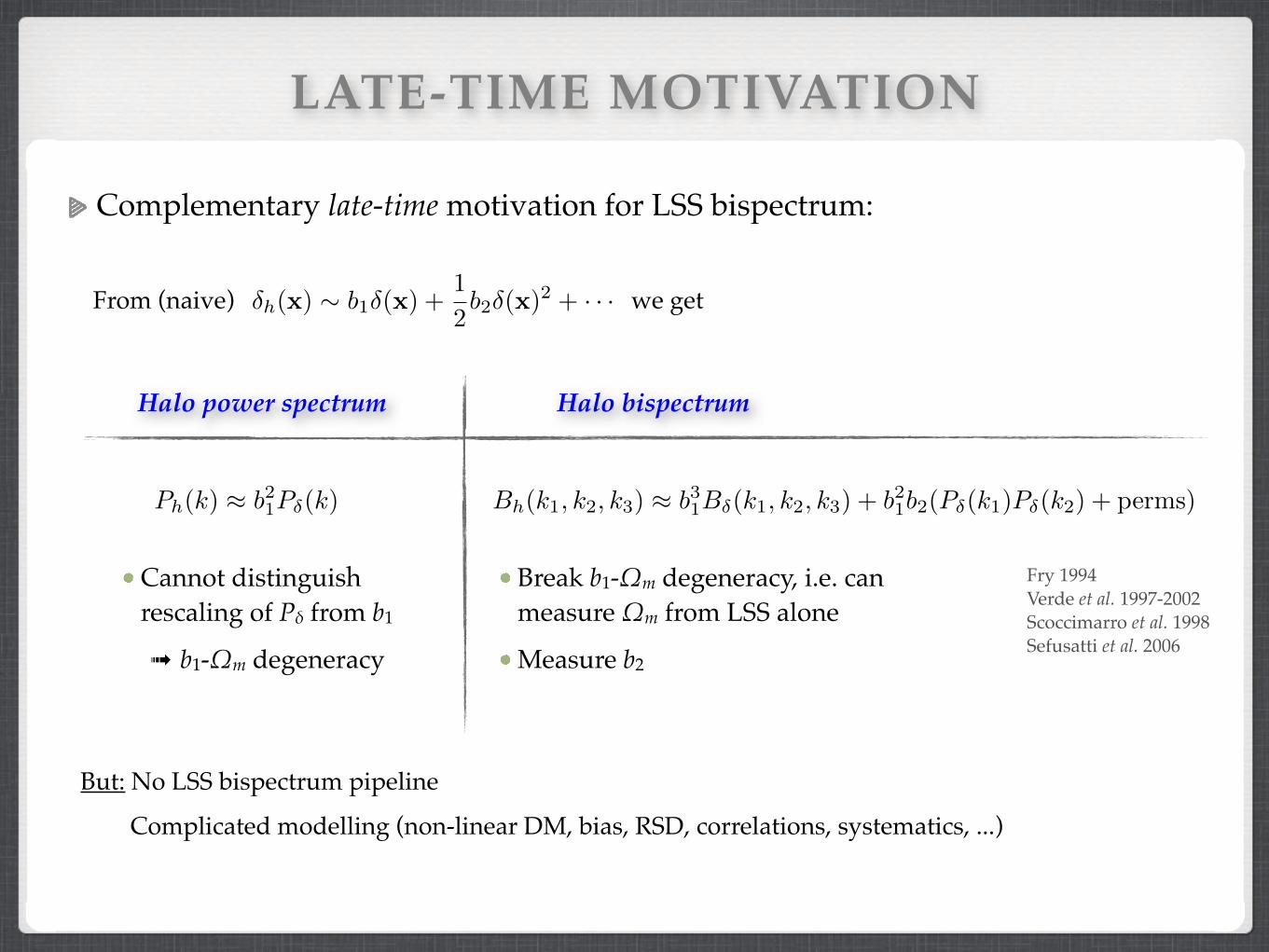
Complementary late-time motivation for LSS bispectrum:
LATE-TIME MOTIVATION
Fry 1994Verde et al. 1997-2002Scoccimarro et al. 1998Sefusatti et al. 2006
But: No LSS bispectrum pipeline
Complicated modelling (non-linear DM, bias, RSD, correlations, systematics, ...)
Ph(k) ⇡ b21P�(k) Bh(k1, k2, k3) ⇡ b31B�(k1, k2, k3) + b21b2(P�(k1)P�(k2) + perms)
Halo power spectrum Halo bispectrum
Break b1-!m degeneracy, i.e. can measure !m from LSS alone
Measure b2
Cannot distinguish rescaling of P" from b1
➟ b1-!m degeneracy
From (naive) we get�h(x) ⇠ b1�(x) +1
2b2�(x)
2 + · · ·

BISPECTRUM
BispectrumPrimary diagnostic for non-Gaussianity because vanishes for Gaussian perturbations
Defined for closed triangles (statistical homogeneity and isotropy)
h�(k1)�(k2)�(k3)i = (2⇡)3�D(k1 + k2 + k3)fNLB�(k1, k2, k3)
non-linear amplitude
bispectrum
k1 k2
k3sum of the two smaller sides ≥ longest side
(every point corresponds to a triangle config.)
)k3
kmax
kmax k1
k2
Bispectrum domain = ‘tetrapyd’(=space of triangle configurations)

BISPECTRUM SHAPES
)
k3
kmax
kmax k1
k2
Squeezed triangles (local shape)
Arises in multifield inflation; detection would rule out all single field models!
Different inflation models induce different momentum dependencies (shapes) of B�(k1, k2, k3)
k2 ⇡ k3 � k1
k1k2
k3
Equilateral triangles
k1 ⇡ k2 ⇡ k3
k3
kmax
kmax k1
k2
k3
kmax
kmax k1
k2
Typically higher derivative kinetic terms, e.g. DBI inflation
Folded triangles
k3 = 2k1 = 2k2
k2
k3
k1
E.g. non-Bunch-Davies vacuum

bispectrum drawn on space of triangle configurations

INITIAL CONDITIONS
Fast and general non-Gaussian initial conditions for N-body simulationsArbitrary (including non-separable) bispectra, diagonal-independent trispectra
This is the only method to simulate structure formation for general inflation models to date
Idea:
↵0= +↵1 +↵2
Note: Actually we plot an orthonormalised version of hereQn
+ · · ·+ ↵nmax
WB
bispectrum drawn on space of triangle configurations
expansion in separable, uncorrelated basis functions(around 100 basis functions represent all investigated
bispectra with high accuracy)
Regan, MS, Shellard, Fergusson PRD 86, 123524 (2012), arXiv:1108.3813
• Generate non-Gaussian density• Convert to initial particle positions and velocities by applying 2LPT to glass
configuration or regular grid (spurious bispectrum at high z decays at low z)• Feed into Gadget3
Application:

Simplest case: local non-Gaussianity
General case: arbitrary bispectrum
Wagner et al 2010
(=2 in local case)WB(k, k0, k00) ⌘ B�(k, k0, k00)
P�(k)P�(k0) + P�(k)P�(k00) + P�(k0)P�(k00)
INITIAL CONDITIONS: MATHS
Aim: Create non-Gaussian field
B�
Fergusson, Regan, Shellard PRD 86, 063511 (2012), arXiv: 1008.1730Regan, MS, Shellard, Fergusson PRD 86, 123524 (2012), arXiv:1108.3813
Requires ~N6 operations in general, but only ~N3 operations if WB was separable:
WB(k, k0, k00) = f1(k)f2(k
0)f3(k00) + perms
full field Gaussian �(x) = �G(x) + �NG(x)
non-Gaussian part
�(x) = �G(x) + fNL(�2G(x)� h�2
Gi)
Expanding WB in separable basis functions gives N3 scaling for any* bispectrum
*Scoccimarro and Verde groups try to rewrite WB analytically in separable form; this works sometimes, but not in general
�NG(k) =fNL
2
Zd3k0d3k00
(2⇡)3�D(k� k0 � k00)WB(k, k
0, k00)�G(k0)�G(k
00)
N =#ptcles
dim⇠ 1000

BISPECTRUM ESTIMATION
Fast and general bispectrum estimator for N-body simulations MS, Regan, Shellard 1207.5678
Measure ~100 fNL amplitudes of separable basis shapes, combine them to reconstruct the full bispectrum
Scales like 100xN3 instead of N6, where N~1000 (speedup by factor ~107)
Can estimate bispectrum whenever power spectrum is typically measured
Validated against PT at high z
Useful compression to ~100 numbers
Automatically includes all triangles
Loss of total S/N due to truncation of basis is only a few percent (could be improved with larger basis; for ~N3 basis functions the estimator would be exact)
Theory
Expansion of theory
N-body
Gravity Excess bispectrum for local NGz=30

BISPECTRUM ESTIMATION: MATHSFergusson, Shellard et al. 2009-2012MS, Regan, Shellard 1207.5678
Likelihood for fNL given a density perturbation δk
Maximise w.r.t. fNL (given a theoretical bispectrum )
Requires ~N6 operations in general, but only ~N3 operations if was separable
➟ Measure amplitudes of separable basis functions
➟ Combine them to reconstruct full bispectrum from the data:
L /Z
d3k1
(2⇡)3d3k2
(2⇡)3d3k3
(2⇡)3
2
641�1
6h�k1�k2�k3i| {z }
/fNLB�
@
@�k1
@
@�k2
@
@�k3
+ · · ·
3
751p
detC
Y
ij
e�12 �
⇤ki
(C�1)ij�kj
/ P�
f̂Btheo
�NL =
1
NfNL
Zd3k
1
(2⇡)3d3k
2
(2⇡)3d3k
3
(2⇡)3(2⇡)3�D(k
1
+ k2
+ k3
)Btheo
� (k1
, k2
, k3
)�k1
�k2
�k3
P�(k1)P�(k2)P�(k3)
Btheo
�
Btheo
�
where , , �Rn ⌘
X
m
�nm�Qm Mr(x) ⌘
Zd3k
(2⇡)3eikx
qr(k)�obskp
kP�(k)�Qm ⌘
Zd3xMr(x)Ms(x)Mt(x)
B̂(k1, k2, k3) =X
n
�Rn
sP�(k1)P�(k2)P�(k3)
k1k2k3Rn(k1, k2, k3)
depends on data

GAUSSIAN
SIMULATIONS
MS, Regan, Shellard 1207.5678
3 realisations of 5123 particles in a L = 1600 Mpc/h box with zinit = 49 and k = 0.004 - 0.5 h/Mpc
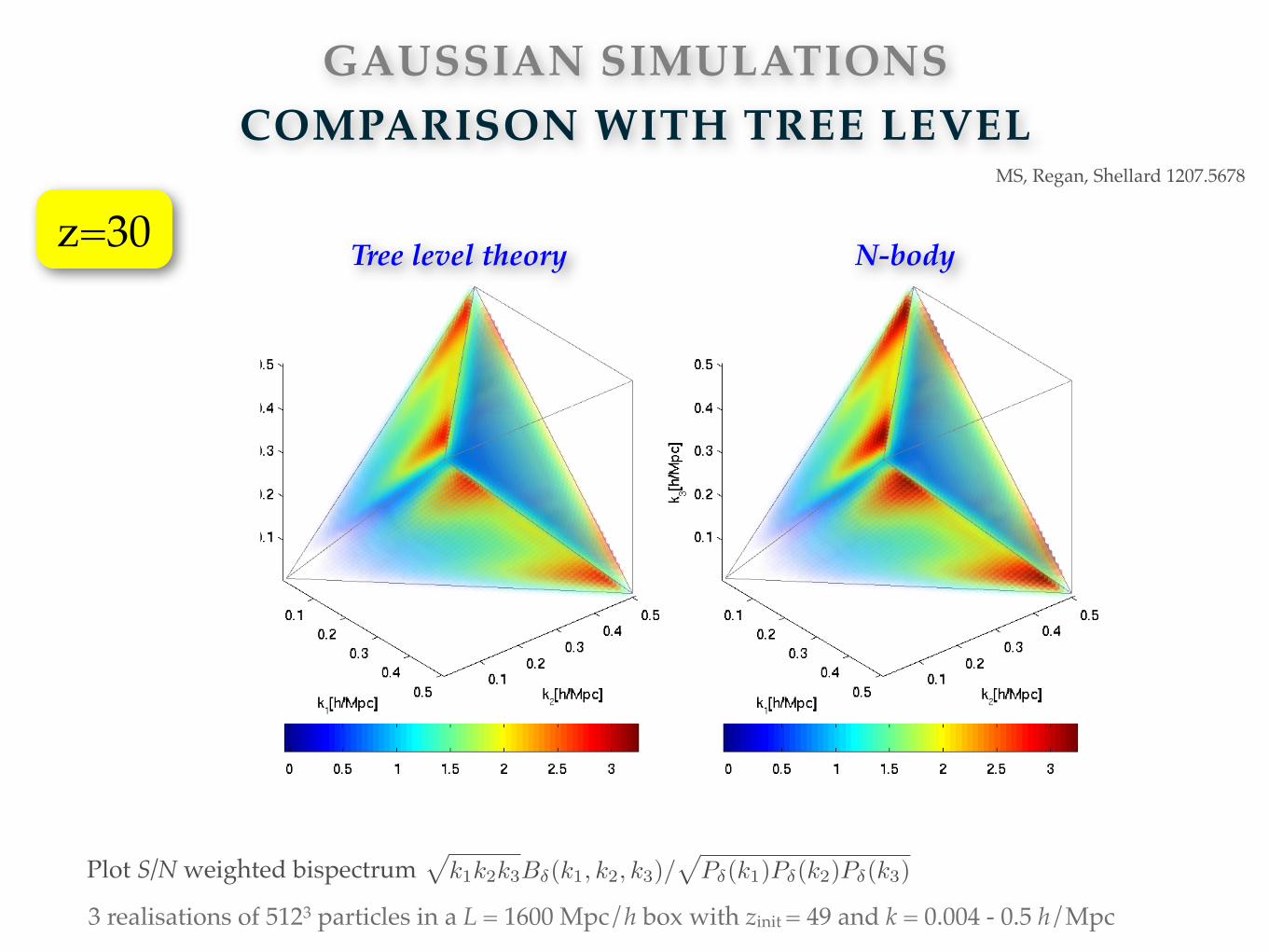
Plot S/N weighted bispectrumpk1k2k3B�(k1, k2, k3)/
pP�(k1)P�(k2)P�(k3)
z=30 Tree level theory N-body
GAUSSIAN SIMULATIONSCOMPARISON WITH TREE LEVEL

MS, Regan, Shellard 1207.5678
3 realisations of 5123 particles in a L = 1600 Mpc/h box with zinit = 49 and k = 0.004 - 0.5 h/Mpc
Plot S/N weighted bispectrumpk1k2k3B�(k1, k2, k3)/
pP�(k1)P�(k2)P�(k3)
Tree level theory N-bodyz=2
GAUSSIAN SIMULATIONSCOMPARISON WITH TREE LEVEL

MS, Regan, Shellard 1207.5678
3 realisations of 5123 particles in a L = 1600 Mpc/h box with zinit = 49 and k = 0.004 - 0.5 h/Mpc
Plot S/N weighted bispectrumpk1k2k3B�(k1, k2, k3)/
pP�(k1)P�(k2)P�(k3)
Tree level theory N-bodyz=0
GAUSSIAN SIMULATIONSCOMPARISON WITH TREE LEVEL
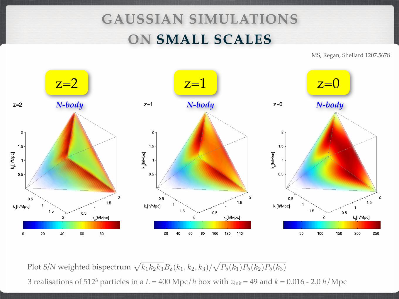
GAUSSIAN SIMULATIONSON SMALL SCALES
MS, Regan, Shellard 1207.5678
3 realisations of 5123 particles in a L = 400 Mpc/h box with zinit = 49 and k = 0.016 - 2.0 h/Mpc
Plot S/N weighted bispectrumpk1k2k3B�(k1, k2, k3)/
pP�(k1)P�(k2)P�(k3)
N-body N-body N-body
z=1 z=0z=2

MS, Regan, Shellard 1207.5678
DM density
GAUSSIAN SIMULATIONSCOMPARISON WITH DARK MATTER
5123 particles in a L = 400 Mpc/h box with zinit = 49 and k = 0.016 - 2 h/Mpc
Plot DM density in (40 Mpc/h)3 subbox and bispectrum signalpk1k2k3B�(k1, k2, k3)/
pP�(k1)P�(k2)P�(k3)
DM bispectrum
22
(a) Dark matter, z = 4 (b) Bispectrum signal, z = 4
(c) Dark matter, z = 2 (d) Bispectrum signal, z = 2
(e) Dark matter, z = 0 (f) Bispectrum signal, z = 0
Figure 10. Left: Dark matter distribution in a (40Mpc/h)3 subbox of one of the G512
400
simulations at redshifts z = 4, 2 and 0, from topto bottom. Right: Measured (signal to noise weighted) bispectrum in the range 0.016h/Mpc k 2h/Mpc, averaged over the simulationon the left and two additional seeds.
40 Mpc/h40
Mpc/h
22
(a) Dark matter, z = 4 (b) Bispectrum signal, z = 4
(c) Dark matter, z = 2 (d) Bispectrum signal, z = 2
(e) Dark matter, z = 0 (f) Bispectrum signal, z = 0
Figure 10. Left: Dark matter distribution in a (40Mpc/h)3 subbox of one of the G512
400
simulations at redshifts z = 4, 2 and 0, from topto bottom. Right: Measured (signal to noise weighted) bispectrum in the range 0.016h/Mpc k 2h/Mpc, averaged over the simulationon the left and two additional seeds.
z=4

MS, Regan, Shellard 1207.5678
DM density
GAUSSIAN SIMULATIONSCOMPARISON WITH DARK MATTER
5123 particles in a L = 400 Mpc/h box with zinit = 49 and k = 0.016 - 2 h/Mpc
Plot DM density in (40 Mpc/h)3 subbox and bispectrum signalpk1k2k3B�(k1, k2, k3)/
pP�(k1)P�(k2)P�(k3)
DM bispectrum
22
(a) Dark matter, z = 4 (b) Bispectrum signal, z = 4
(c) Dark matter, z = 2 (d) Bispectrum signal, z = 2
(e) Dark matter, z = 0 (f) Bispectrum signal, z = 0
Figure 10. Left: Dark matter distribution in a (40Mpc/h)3 subbox of one of the G512
400
simulations at redshifts z = 4, 2 and 0, from topto bottom. Right: Measured (signal to noise weighted) bispectrum in the range 0.016h/Mpc k 2h/Mpc, averaged over the simulationon the left and two additional seeds.
40 Mpc/h40
Mpc/h
22
(a) Dark matter, z = 4 (b) Bispectrum signal, z = 4
(c) Dark matter, z = 2 (d) Bispectrum signal, z = 2
(e) Dark matter, z = 0 (f) Bispectrum signal, z = 0
Figure 10. Left: Dark matter distribution in a (40Mpc/h)3 subbox of one of the G512
400
simulations at redshifts z = 4, 2 and 0, from topto bottom. Right: Measured (signal to noise weighted) bispectrum in the range 0.016h/Mpc k 2h/Mpc, averaged over the simulationon the left and two additional seeds.
z=2

MS, Regan, Shellard 1207.5678
DM density
GAUSSIAN SIMULATIONSCOMPARISON WITH DARK MATTER
5123 particles in a L = 400 Mpc/h box with zinit = 49 and k = 0.016 - 2 h/Mpc
Plot DM density in (40 Mpc/h)3 subbox and bispectrum signalpk1k2k3B�(k1, k2, k3)/
pP�(k1)P�(k2)P�(k3)
22
(a) Dark matter, z = 4 (b) Bispectrum signal, z = 4
(c) Dark matter, z = 2 (d) Bispectrum signal, z = 2
(e) Dark matter, z = 0 (f) Bispectrum signal, z = 0
Figure 10. Left: Dark matter distribution in a (40Mpc/h)3 subbox of one of the G512
400
simulations at redshifts z = 4, 2 and 0, from topto bottom. Right: Measured (signal to noise weighted) bispectrum in the range 0.016h/Mpc k 2h/Mpc, averaged over the simulationon the left and two additional seeds.
40 Mpc/h40
Mpc/h
22
(a) Dark matter, z = 4 (b) Bispectrum signal, z = 4
(c) Dark matter, z = 2 (d) Bispectrum signal, z = 2
(e) Dark matter, z = 0 (f) Bispectrum signal, z = 0
Figure 10. Left: Dark matter distribution in a (40Mpc/h)3 subbox of one of the G512
400
simulations at redshifts z = 4, 2 and 0, from topto bottom. Right: Measured (signal to noise weighted) bispectrum in the range 0.016h/Mpc k 2h/Mpc, averaged over the simulationon the left and two additional seeds.
z=0DM bispectrum

GAUSSIAN SIMULATIONSSUMMARY
Summary Gaussian N-body simulations
z=4
z=0
DM density DM bispectrum signal
pancakes
enhanced equilateral
filaments & clusters
flattened
MS, Regan, Shellard 1207.5678
Measured gravitational DM bispectrum for all triangles down to k=2hMpc-1
Non-linearities mainly enhance ‘constant’ 1-halo bispectrum
Bispectrum characterises 3d DM structures like pancakes, filaments, clusters
Self-similarity(constant contribution appears towards late times at fixed length scale, and towards small scales at fixed time)

NON-GAUSSIAN
SIMULATIONS

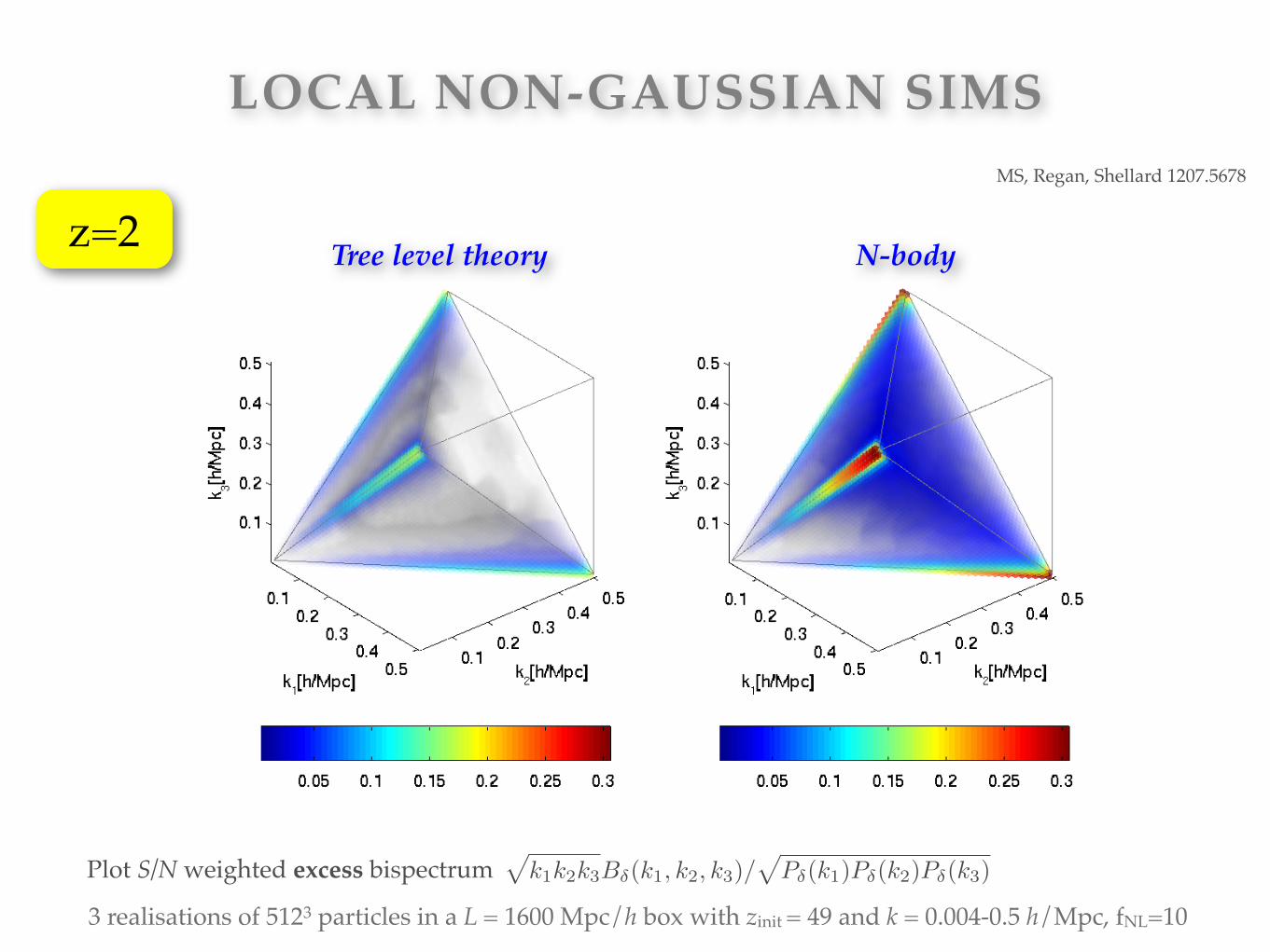
Tree level theory N-body
3 realisations of 5123 particles in a L = 1600 Mpc/h box with zinit = 49 and k = 0.004-0.5 h/Mpc, fNL=10
Plot S/N weighted excess bispectrumpk1k2k3B�(k1, k2, k3)/
pP�(k1)P�(k2)P�(k3)
z=30
LOCAL NON-GAUSSIAN SIMSMS, Regan, Shellard 1207.5678
Tree level theory N-body
3 realisations of 5123 particles in a L = 1600 Mpc/h box with zinit = 49 and k = 0.004-0.5 h/Mpc, fNL=10
Plot S/N weighted excess bispectrumpk1k2k3B�(k1, k2, k3)/
pP�(k1)P�(k2)P�(k3)
z=2
LOCAL NON-GAUSSIAN SIMSMS, Regan, Shellard 1207.5678

Tree level theory N-body
3 realisations of 5123 particles in a L = 1600 Mpc/h box with zinit = 49 and k = 0.004-0.5 h/Mpc, fNL=10
Plot S/N weighted excess bispectrumpk1k2k3B�(k1, k2, k3)/
pP�(k1)P�(k2)P�(k3)
z=0
LOCAL NON-GAUSSIAN SIMSMS, Regan, Shellard 1207.5678

OTHER SHAPES
Excess DM bispectra for other non-Gaussian initial conditions
multiple fields higher derivative operators non-standard vacuum
MS, Regan, Shellard 1207.5678
z=0, kmax=0.5hMpc-1, 5123 particlesNon-linear regime:
Tree level shape is enhanced by non-linear power spectrum
Additional ~constant contribution to bispectrum signal
Quantitative characterisation with cumulative S/N and 3d shape correlations in 1207.5678
multiple fields(local)
higher derivatives(equilateral)
non-standard vacuum(flattened)

Introduce scalar product , shape correlation and norm C
hBi, Bjiest ⌘V
⇡
Z
VB
dk1dk2dk3k1k2k3Bi(k1, k2, k3)Bj(k1, k2, k3)
P�(k1)P�(k2)P�(k3)
h·, ·iest
C(Bi, Bj) ⌘hBi, Bjiestp
hBi, BiiesthBj , Bjiest2 [�1, 1]
if then estimator for cannot find any and vice versa
Babich et al. 2004, Fergusson, Regan, Shellard 2010
||B|| ⌘phB,Biest
||B||
total integrated S/N
|C(B1, B2)| ⌧ 1B1
B2
) hf̂Btheo
NL
i = C(Bdata
� , Btheo
� )||Bdata
� ||||Btheo
� ||projection of data on theory
SIMILARITY OF SHAPES
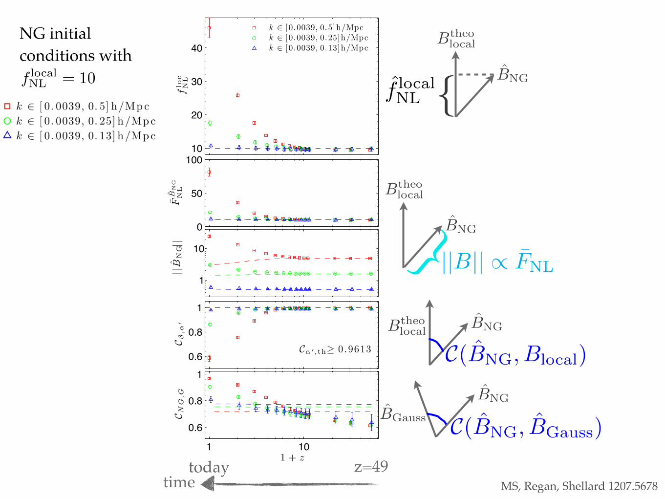
f local
NL
= 10
Btheo
local
B̂NG{NG initial conditions with
10
20
30
40
flo
cN
L
k ! [ 0.0039, 0.5]h/Mpck ! [ 0.0039, 0.25]h/Mpck ! [ 0.0039, 0.13]h/Mpc
0
50
100F̄
B̂N
GN
L
1
10
||B̂
NG||
0.6
0.8
1
C! !, th" 0 .9613
C ",!
!
1 10
0.6
0.8
1
C NG
,G
1 + z
f̂ local
NL
timez=49today
C(B̂NG
, Blocal
)
Btheo
local
B̂NG
Btheo
local
B̂NG}
C(B̂NG, B̂Gauss)
B̂NG
B̂Gauss
||B|| / F̄NL
MS, Regan, Shellard 1207.5678
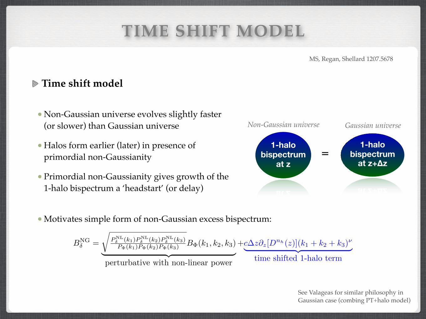
TIME SHIFT MODEL
Time shift model
Non-Gaussian universe evolves slightly faster (or slower) than Gaussian universe
Halos form earlier (later) in presence of primordial non-Gaussianity
Primordial non-Gaussianity gives growth of the 1-halo bispectrum a ‘headstart’ (or delay)
1-halobispectrum
at z
1-halobispectrum
at z+Δz
Gaussian universeNon-Gaussian universe
=
MS, Regan, Shellard 1207.5678
Motivates simple form of non-Gaussian excess bispectrum:
BNG� =
rPNL
� (k1)PNL� (k2)P
NL� (k3)
P�(k1)P�(k2)P�(k3)B�(k1, k2, k3)
| {z }perturbative with non-linear power
+c�z@z[Dnh
(z)](k1 + k2 + k3)⌫
| {z }time shifted 1-halo term
See Valageas for similar philosophy in Gaussian case (combing PT+halo model)

FITTING FORMULAE
Simple fitting formulae for grav. and primordial DM bispectrum shapesValid at 0 ≤ z ≤ 20, k ≤ 2hMpc-1 3d shape correlation with measured shapes is ≥ 94.4% at 0 ≤ z ≤ 20 and ≥ 98 % at z=0 (≥ 99.8% for gravity at 0 ≤ z ≤ 20)
Only ~3 free parameters per inflation model (local, equilateral, flattened, [orthogonal])
MS, Regan, Shellard 1207.5678
Overall amplitude needs to be rescaled by (poorly understood) time-dependent prefactor;extends Gil-Marin et al formula to smaller scales and NG ICs
⌫ ⇡ �1.7
BNG� =
rPNL
� (k1)PNL� (k2)P
NL� (k3)
P�(k1)P�(k2)P�(k3)B�(k1, k2, k3)
| {z }perturbative with non-linear power
+c�z@z[Dnh
(z)](k1 + k2 + k3)⌫
| {z }time shifted 1-halo term
26
100
101
101
102
103
104
1 + z
kBk
(a) Gaussian, kmax
= 0.5h/Mpc
100
101
102
103
104
105
1 + z
kBk
(b) Gaussian, kmax
= 2h/Mpc
Figure 15. Motivation for using the growth function D̄ in the simple fitting formula (64). The arbitrary weight w(z) in Bopt
� =
Bgrav
�,NL
+w(z)(k1
+ k2
+ k3
)⌫ is determined analytically such that C(B̂� , Bopt
� ) is maximal (for ⌫ = �1.7). We plot kBgrav
�,NL
k (black dotted),
kw(z)(k1
+ k2
+ k3
)⌫k (green) and Bgrav
�,const (black dashed) as defined in (14) with fitting parameters given in Table IV, illustrating that
w(z) = c1
D̄nh (z) is a good approximation. The continuous black and red curves show kBfit
� k from (64) and the estimated bispectrum size
kB̂�k, respectively. The overall normalisation can be adjusted with Nfit
as explained in the main text.
Simulation L[Mpc
h
] c1,2 n(prim)
h minz20
C�,↵ C�,↵(z=0)
G512g 1600 4.1⇥ 106 7 99.8% 99.8%
Loc10 1600 2⇥ 103 6 99.7% 99.8%
Eq100 1600 8.6⇥ 102 6 97.9% 99.4%
Flat10 1600 1.2⇥ 104 6 98.8% 98.9%
Orth100 1600 �3.1⇥ 102 5.5 91.0% 91.0%
G512
400
400 1.0⇥ 107 8 99.8% 99.8%
Loc10512400
400 2⇥ 103dD/da 7 98.2% 99.0%
Eq100512400
400 8.6⇥102dD/da 7 94.4% 97.9%
Flat10512400
400 1.2⇥104dD/da 7 97.7% 99.1%
Orth100512400
400 �2.6⇥ 102 6.5 97.3% 98.9%
Table IV. Fitting parameters c1
and nh for the fit (64) ofthe matter bispectrum for Gaussian initial conditions (sim-ulations G512g and G512
400
) and c2
and nprim
h for the fit (69)of the primordial bispectrum (58). The two columns on theright show the minimum shape correlation with the mea-sured (excess) bispectrum in N -body simulations, which wasmeasured at redshifts z = 49, 30, 20, 10, 9, 8, . . . , 0, and theshape correlation at z = 0. For the equilateral case the mini-mum shape correlation can be improved to 99.4% if the term4.6 ⇥ 10�5f
NL
D̄(z)0.5⇥2P�(k1)P�(k2)F
(s)2
(k1
,k2
) + 2 perms⇤
is added to (69).
information. All we require is the time dependence orgrowth rate of the bispectrum amplitude. As a first step,the fitting formula (65) can be normalised to the mea-sured bispectrum size by multiplying it with the normal-isation factor
Nfit ⌘ kB̂kkBfit
� k , (66)
which is shown by the dotted line in the lower panels ofFig. 16. While it varies with redshift between 0.7 and1.4 for kmax = 2h/Mpc, it deviates by at most 8% fromunity for kmax = 0.5h/Mpc. The lower panels also showthe measured integrated bispectrum size kB̂k and thetwo individual contributions to (64) when the normalisa-tion factor Nfit is included. These quantities are dividedby kBgrav
�,NLk for convenience. At high redshifts the totalbispectrum size is essentially given by the contributionfrom Bgrav
�,NL, which equals the tree level prediction for thegravitational bispectrum in this regime. The contribu-tion from Bconst
� dominates at z 2 for kmax = 2h/Mpcwhen filamentary and spherical nonlinear structures areapparent. A similar transition can be seen at later timeson larger scales in Fig. 16a, indicating self-similar be-haviour.
It is worth noting that the high integrated corre-lation between the simple fit (64) and measurementsdoes not imply that all triangle configurations agree per-fectly and sub-percent level di↵erences between shapecorrelations can in principle contain important informa-tion, e.g. about the observationally relevant squeezedlimit which only makes a small contribution to the to-tal tetrapyd integral over the signal-to-noise weighteddark matter bispectrum. However, if we observed thedark matter bispectrum directly, these shapes would behard to distinguish because the shape correlation con-tains the signal-to-noise weighting. Modified shape cor-relation weights and additional basis functions have beenused for better quantitative comparison of the squeezedlimit of dark matter bispectra, but this is left for a futurepublication.
Quality of fit:all z z=0
26
100
101
101
102
103
104
1 + z
kBk
(a) Gaussian, kmax
= 0.5h/Mpc
100
101
102
103
104
105
1 + z
kBk
(b) Gaussian, kmax
= 2h/Mpc
Figure 15. Motivation for using the growth function D̄ in the simple fitting formula (64). The arbitrary weight w(z) in Bopt
� =
Bgrav
�,NL
+w(z)(k1
+ k2
+ k3
)⌫ is determined analytically such that C(B̂� , Bopt
� ) is maximal (for ⌫ = �1.7). We plot kBgrav
�,NL
k (black dotted),
kw(z)(k1
+ k2
+ k3
)⌫k (green) and Bgrav
�,const (black dashed) as defined in (14) with fitting parameters given in Table IV, illustrating that
w(z) = c1
D̄nh (z) is a good approximation. The continuous black and red curves show kBfit
� k from (64) and the estimated bispectrum size
kB̂�k, respectively. The overall normalisation can be adjusted with Nfit
as explained in the main text.
Simulation L[Mpc
h
] c1,2 n(prim)
h minz20
C�,↵ C�,↵(z=0)
G512g 1600 4.1⇥ 106 7 99.8% 99.8%
Loc10 1600 2⇥ 103 6 99.7% 99.8%
Eq100 1600 8.6⇥ 102 6 97.9% 99.4%
Flat10 1600 1.2⇥ 104 6 98.8% 98.9%
Orth100 1600 �3.1⇥ 102 5.5 91.0% 91.0%
G512
400
400 1.0⇥ 107 8 99.8% 99.8%
Loc10512400
400 2⇥ 103dD/da 7 98.2% 99.0%
Eq100512400
400 8.6⇥102dD/da 7 94.4% 97.9%
Flat10512400
400 1.2⇥104dD/da 7 97.7% 99.1%
Orth100512400
400 �2.6⇥ 102 6.5 97.3% 98.9%
Table IV. Fitting parameters c1
and nh for the fit (64) ofthe matter bispectrum for Gaussian initial conditions (sim-ulations G512g and G512
400
) and c2
and nprim
h for the fit (69)of the primordial bispectrum (58). The two columns on theright show the minimum shape correlation with the mea-sured (excess) bispectrum in N -body simulations, which wasmeasured at redshifts z = 49, 30, 20, 10, 9, 8, . . . , 0, and theshape correlation at z = 0. For the equilateral case the mini-mum shape correlation can be improved to 99.4% if the term4.6 ⇥ 10�5f
NL
D̄(z)0.5⇥2P�(k1)P�(k2)F
(s)2
(k1
,k2
) + 2 perms⇤
is added to (69).
information. All we require is the time dependence orgrowth rate of the bispectrum amplitude. As a first step,the fitting formula (65) can be normalised to the mea-sured bispectrum size by multiplying it with the normal-isation factor
Nfit ⌘ kB̂kkBfit
� k , (66)
which is shown by the dotted line in the lower panels ofFig. 16. While it varies with redshift between 0.7 and1.4 for kmax = 2h/Mpc, it deviates by at most 8% fromunity for kmax = 0.5h/Mpc. The lower panels also showthe measured integrated bispectrum size kB̂k and thetwo individual contributions to (64) when the normalisa-tion factor Nfit is included. These quantities are dividedby kBgrav
�,NLk for convenience. At high redshifts the totalbispectrum size is essentially given by the contributionfrom Bgrav
�,NL, which equals the tree level prediction for thegravitational bispectrum in this regime. The contribu-tion from Bconst
� dominates at z 2 for kmax = 2h/Mpcwhen filamentary and spherical nonlinear structures areapparent. A similar transition can be seen at later timeson larger scales in Fig. 16a, indicating self-similar be-haviour.
It is worth noting that the high integrated corre-lation between the simple fit (64) and measurementsdoes not imply that all triangle configurations agree per-fectly and sub-percent level di↵erences between shapecorrelations can in principle contain important informa-tion, e.g. about the observationally relevant squeezedlimit which only makes a small contribution to the to-tal tetrapyd integral over the signal-to-noise weighteddark matter bispectrum. However, if we observed thedark matter bispectrum directly, these shapes would behard to distinguish because the shape correlation con-tains the signal-to-noise weighting. Modified shape cor-relation weights and additional basis functions have beenused for better quantitative comparison of the squeezedlimit of dark matter bispectra, but this is left for a futurepublication.

CONCLUSIONSConclusions
Efficient and general non-Gaussian N-body initial conditions
Fast estimation of full bispectrum
new standard diagnostic alongside power spectrum
Tracked time evolution of the DM bispectrum in a large suite of non-Gaussian N-body simulations
Time shift model for effect of primordial non-Gaussianity
New fitting formulae for gravitational and primordial DM bispectra
See 1108.3813 (initial conditions) 1207.5678 (rest)

COMPARISON WITH OTHER ESTIMATORS
Brute force bispectrum estimator
➟ Slow (107 times slower for 10003 simulation)
Taking only subset of triangle configurations/orientations
➟ Non-optimal estimator: Throw away data (instead, we compress theory domain, not data domain; and we quantify lost S/N~few %)
Binning
➟ Same as our estimator if basis functions are taken as top-hats
➟ But: Not known how much signal is lost with binning (our monomial basis looses few %)
Correlations between triangles and with power spectrum
➟ Potentially easier to get correlations for 100 than for full 3d bispectrum shape
Comparison with theory
➟ Easier with 100 than for full 3d bispectrum shape
Experimental realism:
➟ Need to try... (Planck started with ~7 bispectrum estimators, 3 survived)
�Rn
�Rn
Top Related