


Languages
Pages
Legal


Language Modeling,
N-Gram Models
using examples from the text Jurafsky and Martin, and from slides by Dan Jurafsky

Language Models
• The goal of a Language Model is to assign a probability that a sentence will occur
• Why? • Machine Translation:
– P(high winds tonite) > P(large winds tonite)
• Spell Correction – The office is about fifteen minuets from my house
» P(about fifteen minutes from) > P(about fifteen minuets from)
• Speech Recognition – P(I saw a van) >> P(eyes awe of an)
• + Summarization, question-answering, and many other NLP applications

Language Models
• Goal: compute the probability of a sentence or sequence of words: P(W) = P(w1,w2,w3,w4,w5…wn)
• Related task: probability of an upcoming word: P(w5|w1,w2,w3,w4) condiIonal probability that w5 occurs, given that we know that w1,w2,w3,w4 already occurred.
• A model that computes either of these: P(W) or P(wn|w1,w2…wn-‐1) is called a language model.
• We might call this a grammar because it predicts the structure of the language, but language model is the standard terminology.
3

Chain rule applied Compute the probability of a sentence by computing the joint
probability of all the words conditioned by the previous words P(“its water is so transparent”) = P(its) × P(water|its) × P(is|its water)
× P(so|its water is) × P(transparent|its water is so)
4
€
P(w1w2…wn ) = P(wi |w1w2…wi−1)i∏

Computing Probabilities
• Normally, we just compute the probability that something occurred by counting its occurrences and dividing by the total number
• But there are way too many English sentences in any realistic corpus for this to work! – We’ll never see enough data
5 €
P(the | its water is so transparent that) =
Count(its water is so transparent that the)Count(its water is so transparent that)

Markov Assumption
• Instead we make the simplifying Markov assumption that we can predict the next word based on only one word previous:
• Or perhaps two words previous:
6
Andrei Markov
€
P(the | its water is so transparent that) ≈ P(the | that)
€
P(the | its water is so transparent that) ≈ P(the | transparent that)

N-gram models
• Unigram Model: The simplest case is that we predict a sentence probability just base on the probabilities of the words with no preceding words
• Bigram Model: Prediction based on one previous word:
7
€
P(w1w2…wn ) ≈ P(wi)i∏
€
P(wi |w1w2…wi−1) ≈ P(wi |wi−1)

Bigrams
• Examples of bigrams are any two words that occur together
• In the text: “two great and powerful groups of nations”, the bigrams are “two great”, “great and”, “and powerful”, etc.
• The frequency of an n-gram is the percentage of times the n-gram occurs in all the n-grams of the corpus and could be useful in corpus statistics – For bigram xy:
• Count of bigram xy / Count of all bigrams in corpus
• But in bigram language models, we use the bigram probability to predict how likely it is that the second word follows the first
8

N-gram Models
• We can extend to trigrams, 4-grams, 5-grams – Each higher number will get a more accurate model, but
will be harder to find examples of the longer word sequences in the corpus
• In general this is an insufficient model of language – because language has long-distance dependencies:
“The computer which I had just put into the machine room on the fifth floor crashed.” - the last word crashed is not very likely to follow the word floor, but
it is likely to be the main verb of the word computer
- But we can often get away with N-gram models 9

N-Gram probabilities • For N-Grams, we need the conditional probability:
P(<next word> | <preceding word sequence of length n>) e.g. P ( the | They picnicked by )
• We define this as – the observed frequency (count) of the whole sequence divided by – the observed frequency of the preceding, or initial, sequence
(sometimes called the maximum likelihood estimation (MLE): P(<next word> | <preceding word sequence of length n>) = Count ( <preceding word sequence> <next word>) / Count (<preceding word sequence>)
– Example: Count (They picnicked by the) / Count (They picnicked by)
10

Bigram probabilities
• For bigrams, the MLE estimate is: – The count of the occurrences of the sequence wi-1 wi
divided by the count of the first word wi-1
11
€
P(wi |wi−1) =count(wi−1,wi)count(wi−1)

Example of Bigram probabilities
• Example mini-corpus of three sentences, where we have sentence detection and we include the sentence tags in order to represent the beginning and end of the sentence.
<S> I am Sam </S> <S> Sam I am </S> <S> I do not like green eggs and ham </S>
• Bigram probabilities: P ( I | <S> ) = 2/3 = .67 (probability that I follows <S>) P ( </S> | Sam ) = ½ = .5 P ( Sam | <S> ) = 1/3 = .33 P ( Sam | am ) = ½ = .5 P ( am | I ) = 2/3 = .67
12

More Examples:
• Berkeley Restaurant Project sentences – can you tell me about any good cantonese restaurants close by
– mid priced thai food is what i’m looking for – tell me about chez panisse – can you give me a lisIng of the kinds of food that are available
– i’m looking for a good place to eat breakfast – when is caffe venezia open during the day
13

Raw Bigram Counts from the corpus
• Out of 9222 sentences, showing counts that the word on the leX is followed by the word on the top
14

Bigram probabilities
• Divide/normalize by unigram probabilities:
• Result:
15

Using N-Grams for sentences
( )∏=
−
n
kkk wwP
11|• For a bigram grammar
– P(sentence) can be approximated by multiplying all the bigram probabilities in the sequence
• Example: P(I want to eat Chinese food) =
P(I | <S>) P(want | I) P(to | want) P(eat | to) P(Chinese | eat) P(food | Chinese)

More Bigrams from the restaurant corpus Eat on .16 Eat Thai .03
Eat some .06 Eat breakfast .03
Eat lunch .06 Eat in .02
Eat dinner .05 Eat Chinese .02
Eat at .04 Eat Mexican .02
Eat a .04 Eat tomorrow .01
Eat Indian .04 Eat dessert .007
Eat today .03 Eat British .001
Examples due to Rada Mihalcea

Additional Bigrams
<S> I .25 Want some .04
<S> I’d .06 Want Thai .01
<S> Tell .04 To eat .26
<S> I’m .02 To have .14
I want .32 To spend .09
I would .29 To be .02
I don’t .08 British food .60
I have .04 British restaurant .15
Want to .65 British cuisine .01
Want a .05 British lunch .01

Computing Sentence Probabilities
• P(I want to eat British food) = P(I|<S>) P(want|I) P(to|want) P(eat|to) P(British|eat) P(food|British) = .25×.32×.65×.26×.001×.60 = .000080
• vs. • P(I want to eat Chinese food) = .00015
• Probabilities seem to capture “syntactic'' facts, “world knowledge'' – eat is often followed by a NP – British food is not too popular
• N-gram models can be trained by counting and normalization

In-Class Exercise
20

Why do we need smoothing?
• Every N-gram training matrix is sparse, even for very large corpora ( remember Zipf’s law) – There are words that don’t occur in the training corpus
that may occur in future text – These are known as the unseen words
• Whenever a probability is 0, it will multiply the entire sequence to be 0
• Solution: estimate the likelihood of unseen N-grams and include a small probability for unseen words

Intuition of smoothing (from Dan Klein) • When we have sparse staIsIcs:
• Steal probability mass to generalize beZer
22
P(w | denied the) 3 allegaIons 2 reports 1 claims 1 request
7 total
P(w | denied the) 2.5 allegaIons 1.5 reports 0.5 claims 0.5 request 2 other
7 total
alle
gatio
ns
repo
rts
clai
ms
atta
ck
requ
est
man
outc
ome
…
alle
gatio
ns
atta
ck
man
outc
ome
…alle
gatio
ns
repo
rts
clai
ms
requ
est

Smoothing • Add-one smoothing
– Given: P(wn|wn-1) = C(wn-1wn)/C(wn-1)
– Add 1 to each count: P(wn|wn-1) = [C(wn-1wn) + 1] / [C(wn-1) + V]
• Backoff Smoothing for higher-order N-grams – Notice that:
• N-grams are more precise than (N-1)grams • But also, N-grams are more sparse than (N-1) grams
– How to combine things? • Attempt N-grams and back-off to (N-1) if counts are not available • E.g. attempt prediction using 4-grams, and back-off to trigrams (or
bigrams, or unigrams) if counts are not available
• More complicated techniques exist: in practice, NLP LM use Knesser-Ney smoothing 23

N-gram Model Application - Spell Correction
• Frequency of spelling errors in human typed text varies – 0.05% of the words in carefully edited journals – 38% in difficult applications like telephone directory lookup
• Word-based spell correction checks each word in a dictionary/lexicon – Detecting spelling errors that result in non-words – mesage -> message by looking only at the word in isolation – May fail to recognize an error (real-word errors)
• Typographical errors e.g. there for three • Homonym or near-homonym e.g. dessert for desert, or piece for peace
• Use context of preceding word and language model to choose correct word – Japanese Empirical Navy -> Japanese Imperial Navy

N-gram Model Analysis of Handwritten Sentence
• Optical character recognition has higher error rates than human typists
• Lists of up to top 5 choices of the handwritten word recognizer, with correct choice highlighted
• Using language models with collocational (alarm clock) & syntactic (POS) information, correct sentence is extracted:

Language Modeling Toolkit
• SRI Language Modeling: – hZp://www.speech.sri.com/projects/srilm/
26

More on Corpus Statistics
27
9/9/13 28
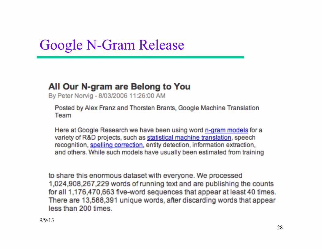
Google N-Gram Release

Example Data
• Examples of 4-gram frequencies from the Google N-gram release – serve as the incoming 92!– serve as the incubator 99!– serve as the independent 794!– serve as the index 223!– serve as the indication 72!– serve as the indicator 120!– serve as the indicators 45!– serve as the indispensable 111!– serve as the indispensible 40!– serve as the individual 234!
29

Google n-gram viewer
• In 2010, Google placed on on-line n-gram viewer that would display graphs of n-gram frequencies of one or more n-grams, based on a corpus defined from Google Books – http://ngrams.googlelabs.com/ – And see also the “About Google Books NGram Viewer”
link
30
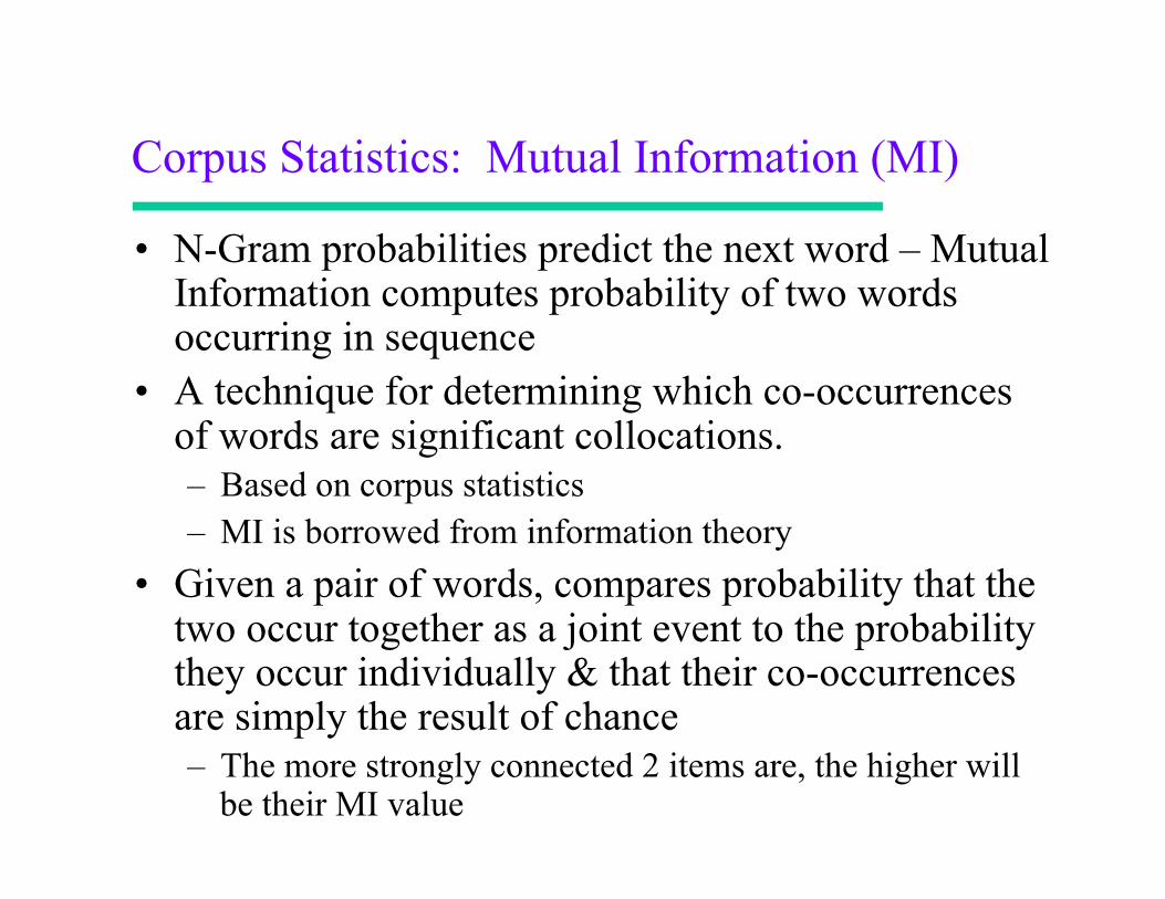
Corpus Statistics: Mutual Information (MI)
• N-Gram probabilities predict the next word – Mutual Information computes probability of two words occurring in sequence
• A technique for determining which co-occurrences of words are significant collocations. – Based on corpus statistics – MI is borrowed from information theory
• Given a pair of words, compares probability that the two occur together as a joint event to the probability they occur individually & that their co-occurrences are simply the result of chance – The more strongly connected 2 items are, the higher will
be their MI value

Mutual Information
• Based on work of Church & Hanks (1990), generalizing MI to apply to words in sequence – They used terminology Association Ratio
• P(x) and P(y) are estimated by the number of observations of x and y in a corpus and normalized by N, the size of the corpus
• P(x,y) is estimated by the number of times that x is followed by y in a window of w words
• Mutual Information: I (x,y) = log2 ( P(x,y) / P(x) P(y) )

MI values based on 145 WSJ articles
x freq (x) y freq (y) freq (x,y) MI Gaza 3 Strip 3 3 14.42 joint 8 venture 4 4 13.00 Chapter 3 11 14 3 12.20 credit 15 card 11 7 11.44 average 22 yield 7 5 11.06 appeals 4 court 47 4 10.45 ….. said 444 it 346 76 5.02
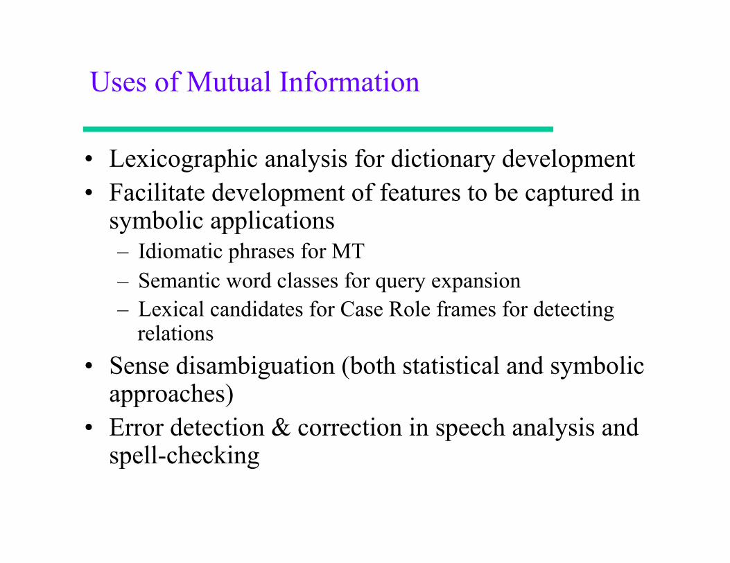
Uses of Mutual Information
• Lexicographic analysis for dictionary development • Facilitate development of features to be captured in
symbolic applications – Idiomatic phrases for MT – Semantic word classes for query expansion – Lexical candidates for Case Role frames for detecting
relations • Sense disambiguation (both statistical and symbolic
approaches) • Error detection & correction in speech analysis and
spell-checking
Top Related
