


Languages
Pages
Legal

2/20/12
1
6.02 Spring 2012 Lecture 3, Slide #1
6.02 Spring 2012 Lecture #3
• Errors in communication • Redundancy with coding (intro)
6.02 Spring 2012 Lecture 3, Slide #2
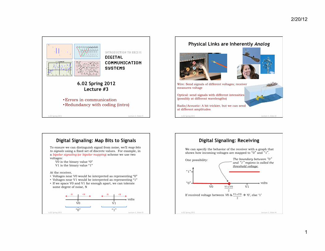
Physical Links are Inherently Analog
Wire: Send signals of different voltages; receiver measures voltage Optical: send signals with different intensities (possibly at different wavelengths) Radio/Acoustic: A bit trickier, but we can send at different amplitudes
6.02 Spring 2012 Lecture 3, Slide #3
Digital Signaling: Map Bits to Signals To ensure we can distinguish signal from noise, we’ll map bits to signals using a fixed set of discrete values. For example, in a bipolar signaling (or bipolar mapping) scheme we use two voltages:
V0 is the binary value “0” V1 is the binary value “1”
At the receiver, • Voltages near V0 would be interpreted as representing “0” • Voltages near V1 would be interpreted as representing “1” • If we space V0 and V1 far enough apart, we can tolerate
some degree of noise, N
V0
+N -N
volts V1
+N -N
“0” “1” 6.02 Spring 2012 Lecture 3, Slide #4
Digital Signaling: Receiving
We can specify the behavior of the receiver with a graph that shows how incoming voltages are mapped to “0” and “1”. One possibility:
V0 volts
V1
“1”
“0” V1+V02
The boundary between “0” and “1” regions is called the threshold voltage.
If received voltage between V0 & à ‘0’, else ‘1’
V1+V02
2/20/12
2
6.02 Spring 2012 Lecture 3, Slide #5
Packaging Messages for Transmission and Reception
Digitize (if needed)
Original source
Source coding
Source binary digits (“message bits”)
Bit stream
COMMUNICATION NETWORK
Render/display, etc.
Receiving app/user
Source decoding
Bit stream
The rest of 6.02 is about the colored oval Simplest network is a single physical comm link We’ll start with that, then get to networks with many links
6.02 Spring 2012 Lecture 3, Slide #6
Single Link Communication Model
Digitize (if needed)
Original source
Source coding
Source binary digits (“message bits”)
Bit stream
Render/display, etc.
Receiving app/user
Source decoding
Bit stream
Channel Coding
(bit error correction)
Recv samples
+ Demapper
Mapper +
Xmit samples
Bits Signals (Voltages)
over physical link
Channel Decoding
(reducing or removing bit errors)
End-host computers
Bits
6.02 Spring 2012 Lecture 3, Slide #7
Network Communication Model Three Abstraction Layers: Packets, Bits, Signals
Digitize (if needed)
Original source
Source coding
Source binary digits (“message bits”)
Packets
Render/display, etc.
Receiving app/user
Source decoding
Bit stream
End-host computers
Packetize
Switch Switch Switch
Switch
Buffer + stream
LINK LINK LINK
LINK
Packets à Bits à Signals à Bits à Packets
Bit stream
6.02 Spring 2012 Lecture 3, Slide #8
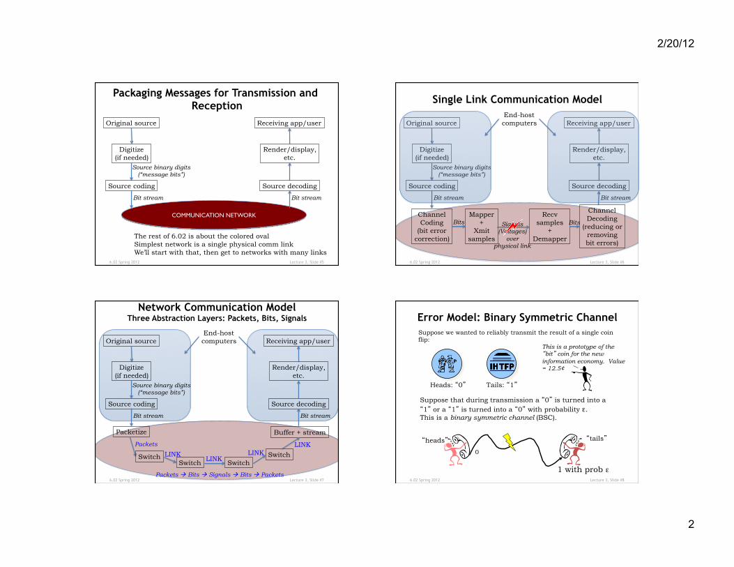
Error Model: Binary Symmetric Channel Suppose we wanted to reliably transmit the result of a single coin flip:
Suppose that during transmission a “0” is turned into a “1” or a “1” is turned into a “0” with probability ε. This is a binary symmetric channel (BSC).
0
1 with prob ε
“heads” “tails”
Heads: “0” Tails: “1”
This is a prototype of the “bit” coin for the new information economy. Value = 12.5¢
2/20/12
3
6.02 Spring 2012 Lecture 3, Slide #9
Performance of Replication Code
Replication factor, n (1/code_rate)
Prob(decoding error) over BSC w/ p=0.01
Code: Bit b coded as bb…b (n times) Exponential fall-off (note log scale) But huge overhead (low code rate)
We can do a lot better!
6.02 Spring 2012 Lecture 3, Slide #10
Hamming Distance
The number of bit positions in which the corresponding bits of two encodings of the same length are different
The Hamming Distance (HD) between a valid binary code word and the same code word with e errors is e. The problem with no coding is that the two valid code words (“0” and “1”) also have a Hamming distance of 1. So a single-bit error changes a valid code word into another valid code word… What is the Hamming Distance of the replication code?
1 0 “heads” “tails”
single-bit error
I wish he’d increase his hamming distance
6.02 Spring 2012 Lecture 3, Slide #11
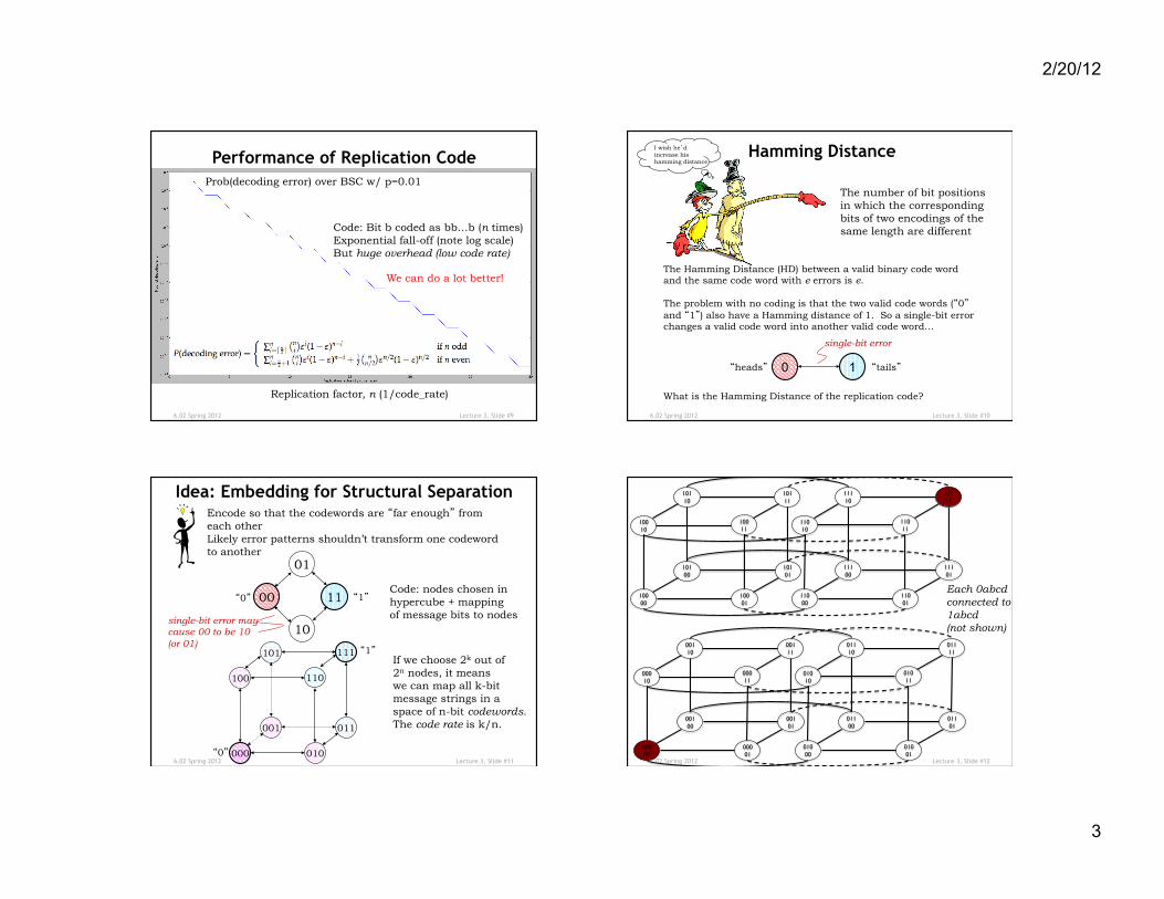
Idea: Embedding for Structural Separation Encode so that the codewords are “far enough” from each other Likely error patterns shouldn’t transform one codeword to another
11 00 “0” “1”
01
10 single-bit error may cause 00 to be 10 (or 01)
110
000 “0”
“1”
100
010
111
001
101
011
Code: nodes chosen in hypercube + mapping of message bits to nodes
If we choose 2k out of 2n nodes, it means we can map all k-bit message strings in a space of n-bit codewords. The code rate is k/n.
6.02 Spring 2012 Lecture 3, Slide #12
01000
01011
01001
01110
01100
01111
01101
01010
00000
00011
00001
00110
00100
00111
00101
00010
11000
11011
11001
11110
11100
11111
11101
11010
10000
10011
10001
10110
10100
10111
10101
10010
Each 0abcd connected to 1abcd (not shown)
2/20/12
4
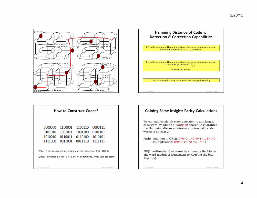
6.02 Spring 2012 Lecture 3, Slide #13
010110
000000
110011
111000
011101
001011
101110
100101
6.02 Spring 2012 Lecture 3, Slide #14
Hamming Distance of Code v. Detection & Correction Capabilities
If D is the minimum Hamming distance between codewords, we can detect all patterns of <= (D-1) bit errors
If D is the minimum Hamming distance between codewords, we can correct all patterns of
or fewer bit errors
!"
!#$
# %
21D
The Hamming distance is satisfies the triangle inequality.
6.02 Spring 2012 Lecture 3, Slide #15
How to Construct Codes?
Want: 4-bit messages with single error correction (min HD=3) Quick, produce a code, i.e., a set of codewords, with this property!
6.02 Spring 2012 Lecture 3, Slide #16
Gaining Some Insight: Parity Calculations
We can add single-bit error detection to any length code word by adding a parity bit chosen to guarantee the Hamming distance between any two valid code words is at least 2. Parity: addition in GF(2): 0+0=0, 1+0=0+1=1, 1+1=0
multiplication: 0*0=0*1=1*0 =0, 1*1=1
GF(2) arithmetic: Can count by summing the bits in the word modulo 2 (equivalent to XOR’ing the bits together).
2/20/12
5
6.02 Spring 2012 Lecture 3, Slide #17
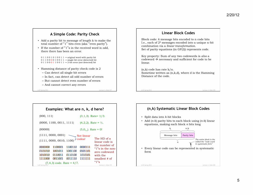
A Simple Code: Parity Check
• Add a parity bit to message of length k to make the total number of “1” bits even (aka “even parity”).
• If the number of “1”s in the received word is odd, there there has been an error. 0 1 1 0 0 1 0 1 0 0 1 1 → original word with parity bit 0 1 1 0 0 0 0 1 0 0 1 1 → single-bit error (detected) bit 0 1 1 0 0 0 1 1 0 0 1 1 → 2-bit error (not detected) bit
• Hamming distance of parity check code is 2 – Can detect all single-bit errors
– In fact, can detect all odd number of errors – But cannot detect even number of errors
– And cannot correct any errors
6.02 Spring 2012 Lecture 3, Slide #18
Linear Block Codes
Block code: k message bits encoded to n code bits I.e., each of 2k messages encoded into a unique n-bit combination via a linear transformation. Set of parity equations (in GF(2)) represents code. Key property: Sum of any two codewords is also a codeword à necessary and sufficient for code to be linear. (n,k) code has rate k/n. Sometime written as (n,k,d), where d is the Hamming Distance of the code.
6.02 Spring 2012 Lecture 3, Slide #19
Examples: What are n, k, d here?
{000, 111} {0000, 1100, 0011, 1111} {00000}
{1111, 0000, 0001}
{1111, 0000, 0010, 1100}
Not linear codes! The HD of a
linear code is the number of “1”s in the non-zero codeword with the smallest # of “1”s
(3,1,3). Rate= 1/3. (4,2,2). Rate = ½. {5,0,_). Rate = 0!
(7,4,3) code. Rate = 4/7. 6.02 Spring 2012 Lecture 3, Slide #20
(n,k) Systematic Linear Block Codes
• Split data into k-bit blocks • Add (n-k) parity bits to each block using (n-k) linear
equations, making each block n bits long
• Every linear code can be represented in systematic form
Message bits Parity bits
k
n The entire block is the called the “code word in systematic form”
n-k
Top Related