


Languages
Pages
Legal


8/3/2019 Kohji Tomita, Haruhisa Kurokawa and Satoshi Murata- Graph automata: natural expression of self-reproduction
http://slidepdf.com/reader/full/kohji-tomita-haruhisa-kurokawa-and-satoshi-murata-graph-automata-natural 1/14
Physica D 171 (2002) 197–210
Graph automata: natural expression of self-reproduction
Kohji Tomita a,∗, Haruhisa Kurokawa a, Satoshi Murata b,1
a National Institute of Advanced Industrial Science and Technology (AIST), 1-2 Namiki, Tsukuba 305-8564, Japanb Department of Computational Intelligence and Systems Science, Interdisciplinary Graduate School of Science and Technology, Tokyo
Institute of Technology, 4259 Nagatsuda, Midori-ku, Yokohama 226-8502, Japan
Received 6 March 2002; received in revised form 14 May 2002; accepted 16 July 2002
Communicated by A. Doelman
Abstract
A variety of models of self-reproduction process have been proposed since von Neumann initiated this field with his
self-reproducing automata. Almost all of them are described within the framework of two-dimensional cellular automata.
They are heavily dependent on or limited by the peculiar properties of the two-dimensional lattice spaces. But such properties
are irrelevant to the essential nature of self-replication. In this paper, we introduce a new framework called “graph automata”
to obtain a natural description of complicated spatio-temporal developmental processes such as self-reproduction. The most
advantageous point of this methodology is that it is not restricted to particular lattice space. As an illustrative example, a
self-reproduction of Turing machine, which requires very long description by conventional cellular automata, is shown in a
simple and straightforward formulation. Graph automata provide a new tool to approach important scientific problems such
as evolution of morphology, and also to give the basis of self-reproducing and self-repairing artifacts.
© 2002 Elsevier Science B.V. All rights reserved.
PACS: 87.10.+e
Keywords: Self-reproduction; Cellular automata; Self-organization; Emergence; Turing machine
1. Introduction
Self-reproduction, one of the most mysterious prop-
erties of life, has attracted many researchers for a long
time. After von Neumann had become interested in
logical representation of self-reproduction processes
about a half-century ago [1], it has been an object
of theoretical studies [2,3]. The motivation of those
works is no doubt desire to understand the founda-
∗ Corresponding author. Tel.: +81-298-617126;
fax: +81-298-617091.
E-mail addresses: [email protected] (K. Tomita), kurokawa-
[email protected] (H. Kurokawa), [email protected] (S. Murata).1 The work of this author was partly supported by the Sumitomo
Foundation (No. 010145).
tion of self-reproduction process in terms of systems
science. But it is also believed that understanding the
logic of self-replication is necessary to realize molec-
ular or nano-scale machines, because conventional se-
rial production methodology is no longer useful, and
massive parallelism of them requires auto-catalytic
production of machines [4]. Self-replication principle
is also applicable to other fields such as architecture
for self-repairable computers [5,6].
von Neumann designed a self-reproducing machine
within the framework of two-dimensional cellular au-
tomata. It is built on two-dimensional regular lattice,
where each cell has 29 states. The state of each cell
is rewritten according to the state transition rules,
which refers to five neighborhoods including itself.
0167-2789/02/$ – see front matter © 2002 Elsevier Science B.V. All rights reserved.
P I I : S 0 1 6 7 - 2 7 8 9 ( 0 2 ) 0 0 6 0 1 - 2

8/3/2019 Kohji Tomita, Haruhisa Kurokawa and Satoshi Murata- Graph automata: natural expression of self-reproduction
http://slidepdf.com/reader/full/kohji-tomita-haruhisa-kurokawa-and-satoshi-murata-graph-automata-natural 2/14
198 K. Tomita et al. / Physica D 171 (2002) 197–210
The machine consists of a universal constructor, and
a tape that contains all the necessary information to
rebuild the whole structure. The constructor interprets
instructions on the tape and builds a new machineat another place by extending a component called a
constructing arm. Indeed von Neumann’s purpose to
investigate the possible formal framework for evolv-
able machines was achieved, but the machine was too
complicated. It requires 200,000 cells, and even now,
the complete simulation of the machine has not been
conducted. (Recently, an implementation was given
by Pesavento [7] based on an extension of the state
transition rules.) Codd [8] succeeded to reduce the
necessary number of states per cell to 8, but the total
number of cells even increased to 100,000,000. Later,
Takahashi and Hayasako [9] obtained a solution of
41-state, 20,000-cell composition, by introducing a
two-layer lattice system.
In 1984, Langton designed a new type of self-
replicating machine. He obtained much simpler com-
position of self-replicating system (7-state, 86-cell)
by giving up universal construction capability of pre-
vious models [10]. His self-replicating loop is based
on Codd’s sheathed path for signal propagation. He
designed a special instruction sequence to replicatethe whole structure and contained it in the sheath.
Reggia et al. [11] considered symmetry requirements
for the rules and found an unsheathed self-replicating
loop with 6-state, 5-cell, believed to be the smallest
at this moment. Chou and Reggia [12] also showed
that self-replicating structures could emerge from
randomly distributed initial patterns.
On the other hand, Perrier et al. [13] rearrange the
Langton-type self-replication loop to regain the com-
putation capability. They attached two strands to the
loop storing program and data, and succeeded to em-
bed universal Turing machine in very small cell space
proportional to program and data length. However,
it still requires 63 states and 8503 rules. Meanwhile,
Chou and Reggia solved an NP-complete problem,
the satisfiability problem, by introducing competition
among simple self-replicating loops, each of them
carrying different candidates for the solution [14].
Other than these, various formulations of cellular
automata such as asynchronous, heterogeneous and
stochastic cellular automata have been proposed but
are omitted here.
All of the above models are built within the two-
dimensional cellular automata. The simple formalismof cellular automata is quite suitable for both anal-
ysis and synthesis. It brings its ability into full play
when it is applied to field dynamics problems like
fluid flow or reaction–diffusion. However, we think it
is not necessarily the best framework to describe the
self-reproduction processes.
Particular properties of two-dimensional lattice
space obstruct natural expression of self-reproduction
processes. Following are two general restrictions ((1)
and (2)) and two technical disadvantages ((3) and (4))
of the lattice spaces.
(1) Fixed topology. Connection topology among the
cells is restricted to predetermined homogeneous
lattice. Variable resolution is impossible on a reg-
ular lattice.
(2) Difficulty of representing closed space. Biologi-
cal phenomena like embryonic development oc-
cur in finite closed space. Such phenomena cannot
be expressed by many cellular automata, because
they need endless space. We can define cellularautomata on a sphere or a torus, however, the size
of the space cannot be changed.
(3) It is difficult to synchronize between remote com-
ponents. Connecting parts by wires is quite easy
in ordinary space, but very difficult in cellular
space. Since the speed of signal propagation is not
more than one cell per one time step, elaborate
design of relative locations of components and
path lengths is required. For example, von Neu-
mann built a special component just for crossing
independent signals.
(4) It requires room for replicated object . The third
requirement imposes a lot of work to avoid an
overlap between the original and daughter pat-
terns. von Neumann devised the construction arm
for this purpose. In Langton’s self-replication,
the loops leave empty sheaths like coral polyp.
Reggia’s smallest self-replicating pattern cannot
repeat the process more than three times because
of the overlap.

8/3/2019 Kohji Tomita, Haruhisa Kurokawa and Satoshi Murata- Graph automata: natural expression of self-reproduction
http://slidepdf.com/reader/full/kohji-tomita-haruhisa-kurokawa-and-satoshi-murata-graph-automata-natural 3/14
K. Tomita et al. / Physica D 171 (2002) 197–210 199
A method called L-system gives a clue to resolve
these difficulties of cellular automata. L-system is a
method based on the term-rewriting grammar, which
can capture developmental processes of various plantshapes [15,16]. Although it is suitable for describing
tree structures, graphs including closed loops are dif-
ficult to describe. Map L-system has been proposed to
overcome this problem [17]. Although it can describe
a planar cell division process, it requires elaborate rule
design. Doi [18] proposed another formulation called
graph development system. In this system, an inci-
dence matrix represents objective topological struc-
ture, and a submatrix in the whole matrix is rewritten
by the grammar corresponding to local topological
change among the elements. In the sense that these
methods can describe not only state transitions, but
also topological changes of the structure, they have
stronger power of expression than cellular automata.
Although L-system and its variants allow various
patterns of topological change, the regularity of for-
mulation is sacrificed. Namely, the number of related
elements and premised connectivity pattern for a
rewriting rule varies case by case. It is very difficult
to apply L-system and its variants to a systematic
design problem of complex systems.In this paper, we propose a new framework called
“graph automata”, which is both flexible in topology
and regular in formulation. The idea was first pre-
sented in [19]. Graph automata is a class of automata
including formal rules for cell division, cell commu-
tation and cell annihilation in addition to ordinary
state transition rules. Since the graph automata are not
constrained to a particular lattice system, it is able to
describe processes with changing number of elements
and topology among them like the L-system. On the
other hand, its formulation is homogeneous similar to
cellular automata, thus suitable to systematic design.
In terms of rewriting of graphs, there has been lots
of research in the area of graph grammars [20]. But
many of them focus mainly on general properties or
computational aspects of the systems, and realization
of self-replicating systems has not been considered so
far.
The rest of this paper is organized as follows. In
Section 2, we give the formulation of graph automata
with some illustrative examples. In Section 3, we
demonstrate its power of expression by showing a
simple composition of self-reproducing Turing ma-
chine, which requires lengthy description by usingconventional cellular automata. Simulation result of
the self-reproducing process is also shown. Section 4
concludes the paper.
2. Formulation of graph automata
In the cellular automata, cells with discrete states
form a lattice and transition of each cell state is deter-
mined by the states of neighbors. For this transition,
lattice structure is not necessary, but each cell needs
to have a certain constant number of neighbors. In
graph automata, all cells (we call them nodes here-
after) have three neighbors. Multiple links between
the same two nodes are allowed. In this paper, we
consider a class of graphs that can be projected onto
a planar graph. This constraint of three neighbors is
satisfied by many structures such as endless planar
honeycomb, tetrahedron, cube, dodecahedron and
fullerene.
Nodes are connected to neighbors via links, andvarious rules to change their states and topology are
applied. We define finite states on nodes, which is
taken from an arbitrary finite set of symbols. At each
node, a cyclic order of links is defined, and all the
nodes are assumed to have the same rotational di-
rection of the cyclic order on the planar graph. The
graph rewriting rules are designed so that the graph
is always kept planar and the directions of the cyclic
orders are conserved.
The constant number of neighbors enables us to
write rules in a regular form, i.e., each rule is described
by a rule name and at most five symbols as its argu-
ments. This gives great advantage when we design a
large complex system. For instance, we can reuse the
same rule in different situations. It is possible to stack
rules as a subroutine where firing of a rule triggers
cascade of other rules. Three-neighbor connectivity is
the minimum that can generate nontrivial graphs, and
more importantly, it is invariant under the following
graph rewriting operations.
8/3/2019 Kohji Tomita, Haruhisa Kurokawa and Satoshi Murata- Graph automata: natural expression of self-reproduction
http://slidepdf.com/reader/full/kohji-tomita-haruhisa-kurokawa-and-satoshi-murata-graph-automata-natural 4/14
200 K. Tomita et al. / Physica D 171 (2002) 197–210
2.1. Rules of graph automata
At first, we give rules of graph automata and
describe the effect of each rule. There are four kindsof rules: one state transition rule and three graph
rewriting rules (Fig. 1). The state transition rule
changes the state of nodes, and the graph rewriting
rules change the structure of the graph. We represent
these rules as follows:
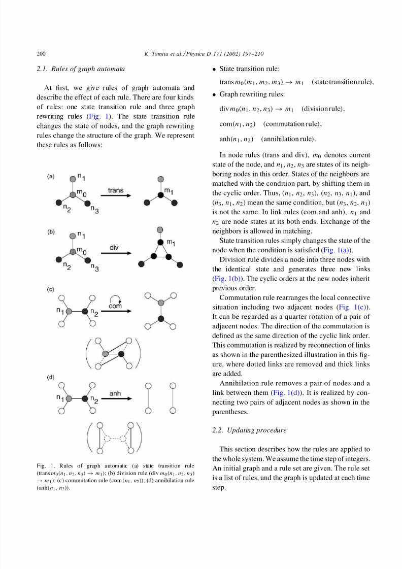
Fig. 1. Rules of graph automata: (a) state transition rule
(trans m0(n1, n2, n3) → m1); (b) division rule (div m0(n1, n2, n3)
→ m1); (c) commutation rule (com (n1, n2)); (d) annihilation rule
(anh(n1, n2)).
• State transition rule:
trans m0(m1, m2, m3) → m1 (state transition rule),
• Graph rewriting rules:
div m0(n1, n2, n3) → m1 (division rule),
com(n1, n2) (commutation rule),
anh(n1, n2) (annihilation rule).
In node rules (trans and div), m0 denotes current
state of the node, and n1, n2, n3 are states of its neigh-
boring nodes in this order. States of the neighbors are
matched with the condition part, by shifting them in
the cyclic order. Thus, (n1, n2, n3), (n2, n3, n1), and
(n3, n1, n2) mean the same condition, but (n3, n2, n1)
is not the same. In link rules (com and anh), n1 and
n2 are node states at its both ends. Exchange of the
neighbors is allowed in matching.
State transition rules simply changes the state of the
node when the condition is satisfied (Fig. 1(a)).
Division rule divides a node into three nodes with
the identical state and generates three new links
(Fig. 1(b)). The cyclic orders at the new nodes inherit
previous order.
Commutation rule rearranges the local connectivesituation including two adjacent nodes (Fig. 1(c)).
It can be regarded as a quarter rotation of a pair of
adjacent nodes. The direction of the commutation is
defined as the same direction of the cyclic link order.
This commutation is realized by reconnection of links
as shown in the parenthesized illustration in this fig-
ure, where dotted links are removed and thick links
are added.
Annihilation rule removes a pair of nodes and a
link between them (Fig. 1(d)). It is realized by con-
necting two pairs of adjacent nodes as shown in the
parentheses.
2.2. Updating procedure
This section describes how the rules are applied to
the whole system. We assume the time step of integers.
An initial graph and a rule set are given. The rule set
is a list of rules, and the graph is updated at each time
step.

8/3/2019 Kohji Tomita, Haruhisa Kurokawa and Satoshi Murata- Graph automata: natural expression of self-reproduction
http://slidepdf.com/reader/full/kohji-tomita-haruhisa-kurokawa-and-satoshi-murata-graph-automata-natural 5/14
K. Tomita et al. / Physica D 171 (2002) 197–210 201
To update the graph automata, we apply only node
rules (trans and div) at even time steps, and link rules
(com and anh) at odd time steps. Rules are executed
synchronously for all the nodes or links. If severalrules are applicable to the same node, i.e., if the left-
hand side of several rules matches, predetermined pri-
ority (listing order in the rule table) determines which
rule to fire. Because applying either commutation or
annihilation to adjacent links causes inconsistency,
all such applications are suppressed. This lateral in-
hibition is realized in several ways in a local manner.
One is to see a wider area covering the next neigh-
bors to confirm that neighboring links do not satisfy
the condition of any rule. Another is to execute the
Fig. 2. Flexible resolution. Uniform honeycomb lattice with arbitrary resolution is obtained when division and commutation rules are
alternately applied.
process in two steps. First, each link raises a flag if
a rule condition is satisfied, and then, if any of the
four neighboring links does not raise the flag, the
link actually execute the rule. We adopt the latter inthe following simulation. By these restrictions, the
updating process becomes completely deterministic.
2.3. Simulation of graph automata
When we are to design the elaborate graph struc-
ture and rule set, the development process becomes
complicated and some mechanical aid is necessary
to visualize the process. For this purpose, we devel-
oped a simulator of the development process of graph

8/3/2019 Kohji Tomita, Haruhisa Kurokawa and Satoshi Murata- Graph automata: natural expression of self-reproduction
http://slidepdf.com/reader/full/kohji-tomita-haruhisa-kurokawa-and-satoshi-murata-graph-automata-natural 6/14
202 K. Tomita et al. / Physica D 171 (2002) 197–210
automata. Such a simulator is useful also to verify the
designed rule sets.
In this simulator, the method to display graphs
is important to grasp the graph structure. Becausegraphs used in this paper are planer, there are many
ways to show them on a plane. But it is not easy to
draw the graphs on a plane without overlapping of the
links. Thus we take a different approach to simplify
the procedure.
The graphs are embedded in the three-dimensional
Euclidean space, and drawn by wireframes on the sur-
face of a sphere (or a balloon). For simplicity, a link
is assumed to be a spring with a damping characteris-
tic. By applying appropriate pressure force inside the
balloon, natural wireframe shapes can be generated
according to the development process, as shown later
in Figs. 3(a) and 6.
2.4. Illustrative examples
Here, simple examples are shown to explain the
potential of graph automata.
Fig. 3. Generation of repetitive structure. Initial state is a heterogeneous tetrahedron: (a) structure; (b) rule.
(a) Flexible resolution. Uniform honeycomb lattice
with arbitrary resolution is obtained when di-
vision and commutation are alternately applied
(Fig. 2).(b) Generation of repetitive structure. From a het-
erogeneous tetrahedron (where all the nodes have
different states), a spherical graph is generated
by a rule set similar to (a). Then it continues
to extend four arms with repetitive structure
(Fig. 3(a)). The process is described by 22 rules
(Fig. 3(b)).
(c) Minimal self-replication. Self-replication seque-
nce for heterogeneous tetrahedron (where all the
nodes have different states) is designed (Fig. 4(a)).
It requires two additional intermediate states and
19 rules (Fig. 4(b)). The whole structure and infor-
mation on the nodes is replicated after the eighth
step. (No rules were applied at time steps 0, 3 and
5.) Note that this replicating process is repeated
arbitrarily many times. Although frameworks are
different, this 4-cell solution is even smaller than
Reggia’s 5-cell record.

8/3/2019 Kohji Tomita, Haruhisa Kurokawa and Satoshi Murata- Graph automata: natural expression of self-reproduction
http://slidepdf.com/reader/full/kohji-tomita-haruhisa-kurokawa-and-satoshi-murata-graph-automata-natural 7/14
K. Tomita et al. / Physica D 171 (2002) 197–210 203
Fig. 4. Minimal self-replication: (a) process of minimal self-replication. ‘ex’ denotes state exchange between neighboring nodes that is
done by simultaneous execution of state transition at adjacent nodes. Commutation rules and annihilation rules in step 7 are executed
simultaneously; (b) rule.
3. Design of self-reproducing Turing machine
A Turing machine is a mathematical model of com-
putation [21], which is composed of one-dimensional
tape of infinite length and a moving head. The tape is
divided into squares and each square contains a sym-
bol from a finite set. At any time, the head is located
at one of the squares, and it can read/write only on
the square. The Turing machine has an internal state
chosen from a finite set. From its internal state and a
symbol on the head location, it decides its operation
to write a new symbol, move the head to the left or
right for one square, and change its internal state.
This rewriting process corresponds to computation. It
is a very simple model, but it can compute any com-
putable function according to Church’s thesis [22].
In graph automata, the Turing machine can be mod-
eled by a simple ladder structure (Fig. 5(a)). The upper
nodes of the ladder correspond to squares of the tape,
and one node in the lower ladder plays the role of the
head. To keep the three-neighbor constraint, both ends
of the ladder (called EOTs (end of tape)) are connected
to form a loop. Although the tape is finite, the struc-
ture can be extended for arbitrary length by division of
EOT if necessary. Each operation of a Turing machine
is realized by several rules in graph automata. Writing

8/3/2019 Kohji Tomita, Haruhisa Kurokawa and Satoshi Murata- Graph automata: natural expression of self-reproduction
http://slidepdf.com/reader/full/kohji-tomita-haruhisa-kurokawa-and-satoshi-murata-graph-automata-natural 8/14
204 K. Tomita et al. / Physica D 171 (2002) 197–210
Fig. 5. Reproduction process of Turing machine.
operation of a new symbol on the tape is realized eas-
ily by state transition because the node is adjacent to
the head node. Head moving operation is realized by
two consecutive steps as follows since the node at the
new location cannot refer to the symbol on the head.
First, the head node becomes a state that represents
the new internal state and the moving direction. Then,
one adjacent node changes its state to the new internal
state. Precise steps and rule construction are given in
Appendix A.
Self-reproduction process of the Turing machine
can be naturally expressed within the framework of
graph automata (Fig. 5). Activation begins at the
location of the head, which causes a chain reaction of
activation, and the activated region is controlled to be
only part of the system. After the propagation of the
activated region from the head position to both EOTs,
the structure is duplicated and separated into two lad-
ders. In the design of the reproduction process, we as-
sume that the process begins when the head becomes

8/3/2019 Kohji Tomita, Haruhisa Kurokawa and Satoshi Murata- Graph automata: natural expression of self-reproduction
http://slidepdf.com/reader/full/kohji-tomita-haruhisa-kurokawa-and-satoshi-murata-graph-automata-natural 9/14
K. Tomita et al. / Physica D 171 (2002) 197–210 205
a special internal state. The outline is as follows, and
the detailed set of rules are given in Appendix B.
Step 1. When the head becomes a special state, the
whole self-reproduction process is triggered.At first, the head node and the corresponding
tape node divide (Fig. 5(a) and (b)).
Step 2. If a neighboring head node or tape node is di-
vided, the neighboring nodes are also divided
(Fig. 5(b) and (c)).
Step 3. By commuting the links, a new ladder struc-
ture is constructed (Fig. 5(c) and (d)).
Step 4. By exchanging the information, tape and
node information is placed in appropriate
positions. Then, unnecessary nodes and linksare annihilated to separate the two ladders
(Fig. 5(c)–(f)).
Step 5. The above steps 2–4 are repeated from the
head position to both EOTs. Some rules are
provided to cope with the special conditions
around the EOTs (Fig. 5(e)–(j)).
Step 6. When the processes in both directions are
finished, the EOTs are commuted and then
annihilated. This makes two identical ladder
structures (Fig. 5(j) and (k)).
Step 7. The original state is restored (Fig. 5(k) and(l)), and the whole replication process can be
repeated again.
Both the necessary number of states and rules
depend on the original Turing machine. For two sym-
bol Turing machines, the process requires 20 states
(including five in the initial state) and 257 rules. The
whole process of this case is verified by computer
simulation (Fig. 6). (In this simulation, only repro-
duction is conducted. To execute it also as a Turing
machine, it suffices to merge the rules.) To our knowl-
edge, this is the smallest model of self-reproducing
system with computational capability.
There are no restrictions on the tape length, and the
same rule set is applicable for any sequence of sym-
bols. This compact description is achieved because
graph automata are free from various restrictions of
cellular automata as mentioned above.
It is also possible to realize self-reproduction of
universal Turing machine. For instance, we can embed
Fig. 6. Simulation.
Minsky’s “small” universal Turing machine [23]. In
this case, 30 states and 955 rules are necessary for the
reproduction process, and 23 states and 745 rules in
addition are required for computation as a universal
Turing machine.
4. Discussion and conclusion
In this paper, we proposed a new framework calledgraph automata for natural description of compli-
cated development processes. It has the following
advantages:
• It is not restricted to a homogeneous lattice space.
• It can express processes that include dynamic
changes in the number and topology of the ele-
ments.
• It can naturally deal with processes in the closed
space.

8/3/2019 Kohji Tomita, Haruhisa Kurokawa and Satoshi Murata- Graph automata: natural expression of self-reproduction
http://slidepdf.com/reader/full/kohji-tomita-haruhisa-kurokawa-and-satoshi-murata-graph-automata-natural 10/14
206 K. Tomita et al. / Physica D 171 (2002) 197–210
• The rules are described in a uniform manner.
In addition to showing that it is Turing complete,
we gave a self-reproducing process of a Turing ma-chine. Such process requires lengthy and complicated
description using cellular automata, but we showed
that natural and compact expression is possible by us-
ing graph automata. Graph automata’s strong power
of expression will provide a new tool to describe vari-
ous complex processes. It is especially suitable to de-
scribe a development process in a closed space, where
the process itself determines its boundary conditions.
In our system, there are two restrictions for simpli-
fication as follows. They were introduced to make the
structure and development process simple at least inthis first stage.
One is the structural restriction. In this paper we
considered planer graphs with three link nodes. Planer
restriction is relaxed by permitting nonplanar initial
states, or introducing new rewriting rules. By four link
model, we can extend our system to the 3D space. We
can consider many ways to extend the structure, but it
will depend on the objects to be modeled in the graph
automata.
The other is in updating process. Lateral inhibitionof link rules and separate updating steps for node and
link rules were assumed. These come mainly from the
requirement to make the updating process determinis-
tic. If we permit the stochastic development, we can
exclude such exceptions by, e.g., local application of
rules instead of synchronous application to the whole
system.
We have the following future work to extend the
framework. First one is the introduction of physical
properties such as the distance between nodes or
physical environment. In this paper we have concen-trated only on the logical relation among elements.
Interaction with the external environment or among
the elements that are not linked together will enable to
express more flexible development processes. Second
is the application of evolutionary computation such
as genetic algorithm. We can evolve the system to
achieve some desired property, since the rule descrip-
tion of graph automata is uniform and it is suitable to
these methods.
Inheriting accumulated knowledge in cellular auto-
mata, graph automata will open a new dimension by
introducing topological freedom to system descrip-
tion. It will throw new light in various subjects inscience and technology, such as morphogenesis of
living systems, artificial life, self-assembling molec-
ular systems, and innovative production method in
nano-scale.
Appendix A. Expression of Turing machine
In order to embed a Turing machine in the graph
automata, it is enough to realize the following three as
rules of graph automata: (1) rules to rewrite symbols of the tape and internal state transition rules in the Turing
machine; (2) rules to move the head; (3) rules to extend
the ladder. We assume that the initial structure that
corresponds to the initial state of the Turing machine
is given. Hereafter, we use the following states of the
nodes:
• EOT: end of the tape.
• NH: nonexistence of the head.
• qi , 0, qi , L, qi , R (for each internal TM state
qi ): existence of the head of internal state qi . L andR indicate the moving direction.
• si (for each TM symbol si ): the tape symbol of
the node.
We assume s0 denotes the blank symbol. Each tape
node at both ends are kept to be of this state.
(1) Tape rewriting and internal state transition. Sup-
pose an instruction quintuple of TM (qi , sj , qk , sl ,
dir), which means ‘if the current state is qi and the
current symbol is sj
, then change to state qk
, write
symbol sl and move to dir’, where dir ∈ {L, R}.
Each instruction is realized by the following
rules.
Rewriting the tape symbols is executed by the
following state transition rule:
transsj (sx , qi , 0, sy ) → sk
where sx and sy denote any tape symbol of the
TM.

8/3/2019 Kohji Tomita, Haruhisa Kurokawa and Satoshi Murata- Graph automata: natural expression of self-reproduction
http://slidepdf.com/reader/full/kohji-tomita-haruhisa-kurokawa-and-satoshi-murata-graph-automata-natural 11/14
K. Tomita et al. / Physica D 171 (2002) 197–210 207
In terms of the head action, at first, we change
the head state to a new one that represents the new
internal state and the moving direction. (The head
motion is explained in the next section.)
transqi , 0(NH, sj , NH) → ql , dir
(2) Head motion. Because the new head state above
includes moving direction, the motion is realized
by two simultaneous state changes by the head
node itself and a adjacent node at the new head
location. It is denoted by the following rules de-
pending only on the set of states and symbols.
(qx and qy denote any internal TM state.)
• Moving rightward:
transqx , R(NH, sy , NH) → NH
trans NH(NH, sx , qy , R) → qy , 0
trans NH(EOT, sx , qy , R) → qy , 0
• Moving leftward:
transqx , L(NH, sy , NH) → NH
trans NH(qx , L, sy , NH) → qx , 0
trans NH(qx , L, sy , EOT) → qx , 0
(3) Tape extension. When the head is adjacent to an
EOT, the ladder is extended by one base by di-
viding the EOT and setting up the initial states to
the two new nodes:
div EOT(sx , EOT, qy , 0) → EOT
div EOT(qx , 0, EOT, sy ) → EOT
trans EOT(EOT, EOT, sx ) → s0
trans EOT(qx , 0, EOT, EOT) → NH
A sequence of rule applications is shown in Fig. 7. By
executing a TM command (qi , sj , qk , sl , R) near the
right EOT, tape rewriting ((a) and (b)), internal state
transition ((a) and (b)), and head motion ((b) and (c))
take place, and then the tape is extended ((c)–(e)) in
succession.
Fig. 7. Embedding of a Turing machine. A Turing machine com-
mand (qi , sj , qk , sl , R) is executed by several steps.
Appendix B. Rule set for self-reproducing Turing
machine
Here we give a complete set of rule schemes for
self-reproduction of a Turing machine. Suppose it
starts self-reproduction when the head becomes a
special state H. Rule schemes according to steps 1–7
in Section 3 are denoted by (1)–(7) in Fig. 8, respec-
tively. si , sj , . . . denotes any tape symbol (we simply

8/3/2019 Kohji Tomita, Haruhisa Kurokawa and Satoshi Murata- Graph automata: natural expression of self-reproduction
http://slidepdf.com/reader/full/kohji-tomita-haruhisa-kurokawa-and-satoshi-murata-graph-automata-natural 12/14
208 K. Tomita et al. / Physica D 171 (2002) 197–210
Fig. 8. Rule set for self-reproduction.

8/3/2019 Kohji Tomita, Haruhisa Kurokawa and Satoshi Murata- Graph automata: natural expression of self-reproduction
http://slidepdf.com/reader/full/kohji-tomita-haruhisa-kurokawa-and-satoshi-murata-graph-automata-natural 13/14
K. Tomita et al. / Physica D 171 (2002) 197–210 209
denote si , sj , . . . by si , sj , . . . ). In addition to
the original states (si , H, NH, EOT), the following
intermediate states are used: EOT, EOT, EOT,
EOT(4)
, EOT(5)
, s
i , s
i , H
, H
, H
, NH
, NH
, ERA.Here, , , etc. are used to generate distinct states
from the original, and ERA denotes a state to be an-
nihilated. Particularly, is used to indicate the states
after the division. The number of states is 20 if the
original Turing machine has two symbols. In the rule
description, Q indicates NH or H. Using these states,
each step of self-reproduction can be described in the
following:
Step 1. When the head becomes a special state H, the
whole self-reproduction process is triggered.
At first, the head node H and the correspond-
ing tape node sj divide into nodes in state H
and sj , respectively (Fig. 5(a) and (b)).
Step 2. If a neighboring head node or tape node is
divided into state si or Q
i , nodes sj and NH
are also divided into s j and NH, respectively.
At the same time, the si and Q
i change its
state to si and Q
i , respectively. Information
of the si and Q
i is exchanged (Fig. 5(b) and
(c)).Step 3. When s
i and sj or Q
i and Qi are adjacent, the
link between them are commuted (Fig. 5(c)
and (d)). This commutation builds a new lad-
der structure.
Step 4. By exchanging the information, tape and node
information is placed in appropriate positions.
More precisely, information from the lower
ladder (H or NH) is copied to the right node,
and information from the upper ladder (si ) is
copied to the left node. At the same time, un-
necessary nodes become ERA in preparation
of the future annihilation (Fig. 5(c) and (d)).
Then, the unnecessary nodes and links are an-
nihilated to separate the two ladders (Fig. 5(e)
and (f)).
Step 5. The above steps 2–4 are repeated until it
reaches both EOTs. Some rules are provided
to cope with the cases around the EOTs. The
left and right EOTs are divided into EOT
and EOT, respectively, and then the upper
EOT and lower EOT are divided again into
EOT (Fig. 5(e)–(j)).
Step 6. When the processes in both directions are fin-
ished, EOT
and EOT
are connected with twoEOT(4). They are commuted and then annihi-
lated (Fig. 5(j) and (k)). (EOT(5) is used as
an intermediate state here.) This makes two
identical ladder structures.
Step 7. The original state is restored (Fig. 5(k) and
(l)), and the whole replication process can be
repeated again.
References
[1] J. von Neumann, The Theory of Self-reproducing Automata,
University of Illinois Press, Urbana, IL, 1966.
[2] M. Sipper, Fifty years of research on self-replication: an
overview, Artif. Life 4 (3) (1998) 237–257.
[3] M. Sipper, J.A. Reggia, Go forth and replicate, Sci. Am.
285 (2) (2001) 26–35.
[4] L.S. Penrose, Self-reproducing machines, Sci. Am. 200 (6)
(1959) 105–114.
[5] D. Mange, D. Madon, A. Stauffer, G. Tempesti, von Neumann
revisited: a Turing machine with self-repair and self-repro-
duction properties, Robot. Auton. Syst. 22 (1) (1997) 35–58.
[6] D. Mange, M. Sipper, A. Stauffer, G. Tempesti, Toward
robust integrated circuits: the embryonics approach, Proc.
IEEE 88 (4) (2000) 516–541.
[7] U. Pesavento, An implementation of von Neumann’s
self-reproducing machine, Artif. Life 2 (4) (1995) 337–354.
[8] E.F. Codd, Cellular Automata, Academic Press, New York,
1968.
[9] I. Takahashi, R. Hayasako, Design and implementation of
self-reproducing automata: mathematical model of life, Trans.
Inform. Process. Soc. Jpn. 31 (2) (1990) 238–248. (in
Japanese).
[10] C.G. Langton, Self-reproduction in cellular automata, Physica
D 10 (1–2) (1984) 135–144.
[11] J.A. Reggia, S.L. Armentrout, H.-H. Chou, Y. Peng, Simple
system that exhibit self-directed replication, Science 259
(1993) 1282–1287.[12] H.-H. Chou, J.A. Reggia, Emergence of self-replicating
structures in a cellular automata space, Physica D 110 (3–4)
(1997) 252–276.
[13] J.-Y. Perrier, M. Sipper, J. Zahnd, Toward a viable,
self-reproducing universal computer, Physica D 97 (4) (1996)
335–352.
[14] H.-H. Chou, J.A. Reggia, Problem solving during artificial
selection of self-replicating loops, Physica D 115 (3–4) (1998)
293–312.
[15] A. Lindenmayer, Mathematical models for cellular interaction
in development. Parts I and II, J. Theoret. Biol. 18 (1968)
280–315.
8/3/2019 Kohji Tomita, Haruhisa Kurokawa and Satoshi Murata- Graph automata: natural expression of self-reproduction
http://slidepdf.com/reader/full/kohji-tomita-haruhisa-kurokawa-and-satoshi-murata-graph-automata-natural 14/14
210 K. Tomita et al. / Physica D 171 (2002) 197–210
[16] P. Prusinkiewicz, A. Lindenmayer, The Algorithmic Beauty
of Plants, Springer, New York, 1990.
[17] A. Nakamura, A. Lindenmayer, K. Aizawa, Some systems
for map generation, in: G. Rozenberg, A. Salomaa (Eds.),
The Book of L, Springer, Berlin, 1986, pp. 323–332.[18] H. Doi, Graph-theoretical analysis of cleavage pattern: graph
developmental system and its application to cleavage pattern
of ascidian egg, Dev. Growth Diff. 26 (1) (1984) 49–60.
[19] S. Murata, K. Tomita, H. Kurokawa, Toward emergent system
synthesis by graph automata, in: Proceedings of the 13th
SICE Symposium on Decentralized Autonomous Systems,
2001, pp. 187–192 (in Japanese).
[20] G. Rozenberg (Ed.), Handbook of Graph Grammars and
Computing by Graph Transformation, Foundations, vol. 1,
World Scientific, Singapore, 1997.
[21] A.M. Turing, On computable numbers, with an application
to the Entscheidungsproblem, Proc. London Math. Soc. Ser.2 42 (2) (1936) 230–265.
[22] A. Church, An unsolvable problem of elementary number
theory, Am. J. Math. 58 (2) (1936) 345–363.
[23] M. Minsky, Computation: Finite and Infinite Machines,
Prentice-Hall, Englewood Cliffs, NJ, 1967.
Top Related