


Languages
Pages
Legal


1
AERODYNAMIC SHAPE OPTIMIZATION OF GUIDED MISSILE BASED ON WIND
TUNNEL TESTING AND CFD SIMULATION
by
Goran J. Ocokoljića, Boško P. Rašuob*, and Aleksandar Benginb a Military Technical Institute, Belgrade, Serbia
b University of Belgrade, Faculty of Mechanical Engineering, Belgrade, Serbia
This paper presents modification of the existing guided missile which was
done by replacing the existing front part with the new five, while the rear
part of the missile with rocket motor and missile thrust vector control system
remains the same. The shape of all improved front parts is completely
different from the original one. Modification was performed based on
required aerodynamic coefficients for the existing guided missile. The
preliminary aerodynamic configurations of the improved missile front parts
were designed based on theoretical and Computational Fluid Dynamics
simulations. All aerodynamic configurations were tested in the T-35 wind
tunnel at the Military Technical Institute (VTI) in order to determine the
final geometry of the new front parts. Three-dimensional Reynolds Averaged
Navier–Stokes numerical simulations were carried out to predict
the aerodynamic loads of the missile based on the finite volume method.
Experimental results of the axial force, normal force and pitching moment
coefficients are presented. The computational results of
the aerodynamic loads of a guided missile model are also given, and agreed
well with.
Key words: experimental aerodynamics, wind tunnel testing, CFD,
aerodynamic coefficients, missile model
1. Introduction
Modern missile configuration designs tend to reduce the area of control surfaces, such as fins and
tails, in order to achieve better aerodynamic performance characteristics in flight. As a result of these
design requirements, stability problems could appear at the speed in the low subsonic regime. For this
case, the wing-store interference and low controllability may cause serious safety problems. Therefore,
investigations of the flow field over missile configurations at the subsonic flow and understanding of
the effect that control surfaces have on the stability characteristics and the development of flow
asymmetries are crucial to efforts in improving the design of future-generation missiles. In all phases
of a missile design it is necessary to know the aerodynamic coefficients as a function of the angle of
attack for different Mach numbers and control deflections. In the preliminary design, an accurate
prediction of the aerodynamic coefficients is necessary for the choice of aerodynamic configuration.
The process of missile design requires the use of a variety of theoretical, experimental and
numerical methods [1],[2]. The experiment comprises the measurement of aerodynamic forces and
moments on the model in the wind tunnel. The Computational Fluid Dynamics (CFD) simulations
play an important role in eliminating preliminary models at the beginning of the design process and
leaving expensive wind tunnel testing for detailed models that are close to the final design.
* Corresponding author, e-mail address: [email protected] Tel: +381638676773

2
This paper presents such a combined experimental and numerical approach to a modification of an
existing guided missile. The original configuration of the missile comprised a shaped-charge warhead
that was to be replaced by a choice of five new, more effective, warheads, while the rear part of the
missile with the rocket motor and missile thrust vector control system were to remain unchanged. As
the aerodynamic shapes, masses and the positions of the centers of gravity of the new warheads
differed significantly from the shape of the original one, substitutions of the warhead would have
resulted in the changes of the aerodynamic characteristics of the missile. There was a requirement,
however, to retain the existing semiautomatic command guidance and missile control system, which
required that the aerodynamic characteristics of the modified missiles had to remain similar to the
original one. This was to be achieved by placing additional aerodynamic surfaces on the front part of
the missiles (i.e. on the new warheads). The new aerodynamic surfaces were to be sized and posi-
tioned so as to return N
C
andm
C
close to the original ones in order that the modified configurations
have the same (or slightly better) maneuverability as the original missile, with a minimum penalty of
drag increase. Several variants of these additional surfaces were designed for each of the new
warheads, and the designs analyzed in CFD simulations. Optimization and selection of the final
geometries of the five new front parts of the missile on the basis of the lift-curve and pitching-
moment-curve slopes and lift/drag ratio decrease were then performed in the wind tunnel testing.
2. Experiment
The data for this investigation was obtained in the T-35 subsonic wind tunnel of VTI. The wind
tunnel is of continual type, closed-circuit facility and capable of operation at a Mach number range of
0.1<M<0.5 at atmospheric pressure, Error! Reference source not found.,[3],[4]. The wind tunnel is
equipped Error! Reference source not found.,[5],[5] with two removable solid wall test sections,
first, a general purpose test section with an external six-component balance/model support and,
second, a test section with a tail sting support system. Each test section has an octagonal cross-section,
with a larger axis of 4.4m and a smaller axis of 3.2m. Cross- sectional area is 11.93m2. The length of
each test section is 5.5m.
Figure 1. Two parts of the original model: Figure 2. The 2M Model.
the rocket body and the front part.
The Mach number regulation is achieved by changing the fan rotation rate and the angle of fan
blades. The value of Reynolds number is up to 12 million/m with a fan. The value of the total pressure
in the test section is 1 bar. Theoretically, the duration of the test is unlimited. The facility is used for
research projects as well as for educational experiments and demonstrations. The GM model shown in
this paper is composed of the front part located in the front part and the rocket motor with the thrust
vector control systems located in the rear part of the missile. Figure 1 presents the Original GM model
3
parts. The original model and the modified versions, named 2M, 2T, 2F, 2ТТ and 2FF model, were
designed and tested in the T-35 wind tunnel. Figure 2 shows the 2M model in the T-35.
Figure 3. The 2T Model. Figure 4. The 2F Model.
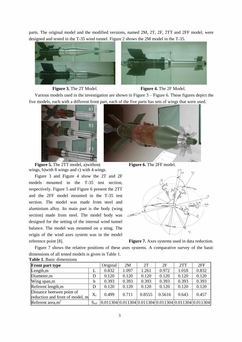
Various models used in the investigation are shown in Figure 3 – Figure 6. These figures depict the
five models, each with a different front part, each of the five parts has sets of wings that were used.
Figure 5. The 2TT model, a)without Figure 6. The 2FF model.
wings, b)with 8 wings and c) with 4 wings.
Figure 3 and Figure 4 show the 2T and 2F
models mounted in the T-35 test section,
respectively. Figure 5 and Figure 6 present the 2TT
and the 2FF model mounted in the T-35 test
section. The model was made from steel and
aluminium alloy. Its main part is the body (wing
section) made from steel. The model body was
designed for the setting of the internal wind tunnel
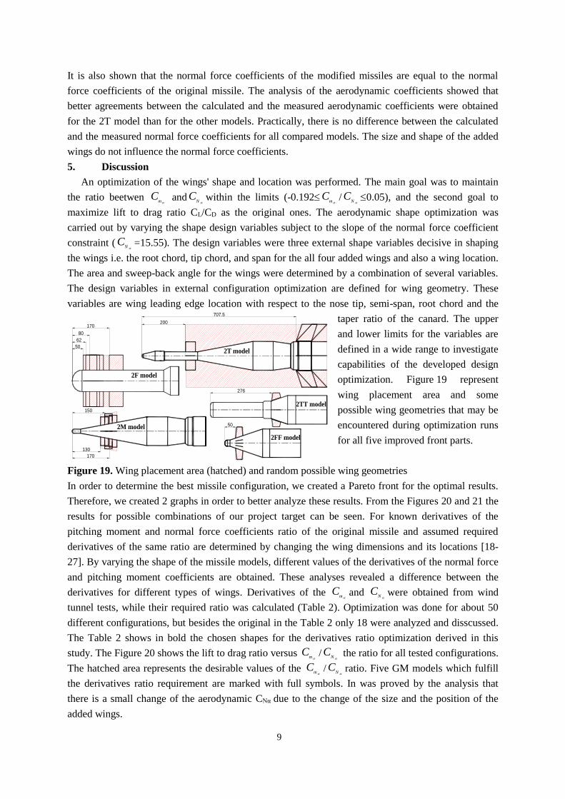
balance. The model was mounted on a sting. The
origin of the wind axes system was in the model
reference point [8]. Figure 7. Axes systems used in data reduction.
Figure 7 shows the relative positions of these axes systems. A comparative survey of the basic
dimensions of all tested models is given in Table 1.
Table 1. Basic dimensions
Front part type Original 2M 2T 2F 2TT 2FF
Length,m L 0.832 1.097 1.261 0.972 1.018 0.832
Diameter,m D 0.120 0.120 0.120 0.120 0.120 0.120
Wing span,m b 0.393 0.393 0.393 0.393 0.393 0.393
Referent length,m D 0.120 0.120 0.120 0.120 0.120 0.120
Distance beetwen point of
reduction and front of model, m Xr 0.499 0.711 0.8555 0.5616 0.643 0.457
Referent area,m2 Sref 0.011304 0.011304 0.011304 0.011304 0.011304 0.011304

4
3. CFD Simulation
The numerical calculations of aerodynamic characteristics of the Original, 2M, 2T and 2F models,
performed using the CFD methods prior to the wind tunnel test campaign, were necessary in order to
estimate the expected loads on the wind tunnel model. The numerical calculation was done in the
FLUENT package, as it allows calculation of the aerodynamic characteristics of complex aerodynamic
shapes [9]-[19]. The solid model of the missile is done in INVENTOR software. Small details like a
gap in the wings, attachments, which do not have a significant effect on aerodynamics, were
removed/approximated for the CFD simulation. Nozzles and tracer that have had significant effect on
the drag calculations are present. Control volume in the shape of an ellipsoid with a major axis three
times greater than the length of the missile (3.8m) and a minor axis sixteen times greater than the
missile diameter (1.9m) and length 5.5m was done by software GAMBIT with the boundary surface
type ’’pressure far field’’. The computational domain inlet is located 15 model body diameter
upstream from the tip of the model nose and the computational domain outlet is located 17 model
body diameter downstream from the model base. Boundary conditions are Mach number, total
pressure, total temperature and turbulence parameters corresponding to the values measured in the
wind tunnel. All model body surfaces are of the ’’wall’’ type. The unstructured mesh composed of
tetrahedral elements is generated in the control volume. The density-based, explicit, compressible,
unstructured-mesh solver was used. A modified form of the k- ε two-equation turbulence model
(realizable k- ε) was used in this study. This turbulence model solves transport equations for the
turbulence kinetic energy, k, and its dissipation rate, ε. In most cases, the computation was initially
done on a coarse mesh with a non-dimensional distance from the model of y+≈30 in order to obtain
the flow field that presented a basis for the grid adaptation. Mesh was generated with respect to
selected mesh growth rate of 1.08, but mentioned growth rate parameter was chosen to vary up to the
value of 1.2. Selection of appropriate growth rate parameter value directly affects total grid size. The
finest grid was defined with total cells number of 2.6 million elements, which corresponds to the
growth rate parameter of 1.08 and with the first wall node placed at y+≈1 in the whole domain for the
angles of attack. This density of the mesh was selected with respect to the sufficient amount of
computer memory and convergence criteria of the calculated aerodynamic coefficients and residuals. It
should be noted that a grid with the total number of cells of about 2.6 million was found to be
sufficient to obtain a good agreement with test results and to ensure convergence of the calculated
aerodynamic coefficients and residuals. Finer grids, between 2.6 million and 4 million elements,
ensured a grid-independent solution. The near-wall region was discretized with 23 layers of prismatic
cells, while the rest of the flow domain consisted of tetrahedral cells. In the regions where y+≈1, the
viscous sub-layer was resolved using a two-layer model for enhanced wall treatment, while the
enhanced wall treatment through the blending of linear and logarithmic laws in the near-wall region
was used in the regions with a higher y+. The cross-sections of the mesh in the computational domain
for the 2M model is given in Figure 8.
The FLUENT commercial flow solver was used to compute the axial and normal force and
pitching moment coefficients and flow-field around the missile model. The viscous computational
fluid dynamic simulations were used to calculate the flow-field around the projectile model in
subsonic flows. The FLUENT (v6.2.16) commercial flow solver is used to compute the base pressure
values and the flow-field around the ATM model. The implicit, compressible, unstructured-mesh

5
solver is used. The three-dimensional, time-dependent, Reynolds-Average Navier-Stokes (RANS)
equations are solved using the finite volume
method (1) and (2):
Figure 8. Cross-section of the mesh in the 2M model vicinity.
The inviscid flux vector F is evaluated by a standard upwind flux-difference splitting. In the implicit
solver, each equation in the coupled set of governing equations is linearized implicitly with respect to
all dependent variables in the set, resulting in a block system of equations. A block Gauss-Seidel point
implicit linear equation solver is used with an algebraic multigrid method to solve the resultant block
system of equations. The computations were performed for the Mach number 0.35 at and the angle of
attack from –10º to 10º. Convergence was determined by tracking the change in the flow residuals and
the aerodynamic coefficients during the solution. The solution was deemed converged when the flow
residuals were reduced at least 2 orders of magnitude and the aerodynamic coefficients changed less
than about 2% over the last 100 iterations.
4. Results
In order to fulfill the requested ratio between the pitching moment and the normal force coefficients,
the wings are added on the forward part of the missile where the front part is located. The aim of the
experiment was to determine the configurations of the wings such that for the same normal force
coefficients as the Original GM get the appropriate coefficient of pitching moment. During the testing,
the shape and position of the wings was changed in order to obtain sufficiently stable model
configurations while being manageable.
Results were obtained by testing at M=0.35
in the T-35 wind tunnel, at the model rolling
angle of `=0˚, and by CFD simulation at
the same conditions. Results are presented
by axial force CA, normal force CN and
pitching moment coefficients Cm. Test
results are given for the model aerodynamic
center, located at the distance of Xr
upstream of the reference plane. The model
reference length for the Reynolds number
calculation is the diameter of the model.
Figure 9. Aerodynamic coefficients of the Original model.
-12 -8 -4 0 4 8 12
-4
-2
0
2
4
CA
Angle of attack [ O
]
CN
T-35 Fluent
CN
Cm
CA
-1.00
-0.75
-0.50
-0.25
0.00
0.25
0.50
0.75
1.00
Cm
0.1
0.2
0.3
0.4
0.5
[ ]V V
WdV F G dA HdVt
(1)
where are
0
, ,
xi
yi
zi
ij
v
u u pi
W F Gv v pj
w w pk
qE E pv
(2)

6
The Original missile model test was used for the aerodynamic coefficient determination, and also
for the determination of the aerodynamic characteristics of the common parts for all configurations of
the rocket motor section. The relation
between the derivatives of the normal
force and the pitching moment
coefficients was adopted for all new
versions of the missile front parts. In the
Figure 9 the diagrams of aerodynamic
coefficients of the Original model are
shown. Having obtained an agreement
between the experimental and the
numerical results on the Original model
configuration, the numerical method was
used in the development of the guided
missile project with improved front parts.
Figure 10. Aerodynamic coeff. of the 2M model.
The results of CFD analysis of the original model
was used to adjust the density of the mesh and the
layout and setting boundary conditions for models
with improved front part. In the Figure 10 the
diagrams of aerodynamic coefficients for the 2M
model are shown.
During the testing of the 2M model two types of
wings were used that were positioned at three
locations.
Figure 11. CFD results of the 2M model.
Configuration of the 2M front part with the type B wings at the location C=150mm from the front of
the model fulfilled all requirements
regarding the relationship between the
normal force and the pitching moment
coeficient. In the diagrams full symbols
mark the final version of the model. The
experimentally and numerically obtained
results for the 2M model with the type B
wings at the location C=150mm were
compared, and the comparisons of the
coefficients as a function of the model
angle of attack are given in graphs in
Figure 11. The maximum difference
between the calculated and the measured
axial force coefficients is about 7.1%. Figure 12. Aerodynamic coeff. of the 2T model.
-12 -8 -4 0 4 8 12
-4
-2
0
2
4
Angel of attack - [ o ]
-1.0
-0.5
0.0
0.5
1.0
2M model T-35 CFD
CN
Cm
CA
CmC
AC
N
0.1
0.2
0.3
0.4
0.5
-12 -8 -4 0 4 8 12
-4
-2
0
2
4
CmCA
wing A, 200mm
wing D, 707,5mm
wing C, 707,5mm
wing B, 200mm
CN 2T model
Angle of attack [ O
]
-1.5
-1.0
-0.5
0.0
0.5
1.0
1.5
0.1
0.2
0.3
0.4
0.5
70
2
70
Wing C45°
R1
3545
2 0.6
55
Wing B
2
0.6
Wing A
45
3545
20°
Wing DR1
2
70
70
-12 -8 -4 0 4 8 12
-4
-2
0
2
4
Angel of attack - [ o ]
-1.0
-0.5
0.0
0.5
1.0
2M model T-35 CFD
CN
Cm
CA
CmC
AC
N
0.1
0.2
0.3
0.4
0.5

7
The maximum difference of the calculated and measured pitching moment coefficients is about
18%. In the Figure 12 the diagrams of aerodynamic coefficients for the 2T model are shown. During
the test four types of wings were used that were positioned at two locations. In the Figure 12 the
sketch of the four tested wings is also shown. Wings A and B are rectangular 45x45(55) with a
diamond cross-sections 2mm thick. Wings C and D are rhombus with sweep angles 45and 20,
respectively. Cross-section of the wings C and D are rectangular with rounded edges of 0.5mm.
Configuration of the 2T front part with the type B wings at the location C=200mm from the front of
the model was adopted. The wind tunnel test results and CFD simulation of the 2T model with the
type B wings at the location C=200mm
were compared in graphs in Figure 13. The
maximum difference between the calculated
and the measured axial force, normal force
and pitching moment coefficients are 10, 2.5
and 4.2%, respectively. In the Figure 14 the
diagrams of aerodynamic coefficients for
the 2F model are shown. During the test one
type of wings was used that was positioned
at four locations.
Figure 13. CFD results of the 2T model.
Configuration of the 2F front part with the type A wings at the location C=170mm from the front of
the model was adopted. The normal force, pitching moment and axial force coefficients calculated by
FLUENT and measured in wind tunnel as a function of the angle of attack for 2F model with the type
A wings at the location C=170mm from the
front of the model are given in Figure 15.
Figure 14. Aerodynamic coeff. of the 2F model. Figure 15. CFD results of the 2F model.
The maximum difference between the calculated and the measured normal force, pitching moment
and axial force, coefficients are 1.8, 12, and 4.8%, respectively. In the Figure 16 and Figure 17 the
diagrams of normal force, pitching moment and axial force coefficients for the 2TT and the 2FF model
are shown. During the 2TT model test one wing type at one positioned location was used. The number
of wings was changed; eight or four wings were used. Configuration of the 2TT front part with
-12 -8 -4 0 4 8 12
-4
-2
0
2
4
CA Cm
Angle of attack - [ o ]
CN
2T model
CFD T-35
CN
Cm
CA
-1,0
-0,5
0,0
0,5
1,0
0,1
0,2
0,3
0,4
0,5
-12 -8 -4 0 4 8 12
-4
-2
0
2
4
63
0.6 2
Wing A
5363
CmCA CN
2F model
Angle of attack [
O ]
wing A, 62mm
wing A, 50mm
wing A, 80mm
without wings
wing A, 170mm
-3
-2
-1
0
1
2
3
0.1
0.2
0.3
0.4
0.5
-12 -8 -4 0 4 8 12
-4
-2
0
2
4
CA CmCN
Angle of attack-[ o ]
2F model
T-35 CFD
CN
Cm
CA
-1,0
-0,5
0,0
0,5
1,0
0,1
0,2
0,3
0,4
0,5

8
8(eight) wings at the location C=276mm from the front of the model was adopted. During the 2FF
model test one wing type positioned at one location C=50mm was used.
-12 -8 -4 0 4 8 12
-4
-2
0
2
4
16°
25
32
0.6
Wing
30
17°
2
2TT model CmCN with 4 wings
without wings
with 8 wings
CA
Angle of attack [ o ]
-2,0
-1,5
-1,0
-0,5
0,0
0,5
1,0
1,5
2,0
0,1
0,2
0,3
0,4
0,5
-12 -8 -4 0 4 8 12
-4
-2
0
2
4
0,2
0,3
0,4
0,5
-1,0
-0,5
0,0
0,5
1,0
2FF model with 8 wings CmCN
CA
Angle of attack [ o ]
CN
Cm
CA
12°
17°
15
50
20
.6Wing
25
Figure 16. Aerodynamic coeff. of the 2TT model. Figure 17. Aerodynamic coeff. of the 2FF model.
Figure 18 shows the dynamic pressure distribution on the GM models body. It can be observed that
the dynamic pressure profiles are symmetric in the pitching and yawing plane when AoA=0O.
Figure 18. Dynamic pressure distribution on the GM models surface.
In the pressure contour, it can be easily found that there are least dynamic pressure areas at the front
of the body, especially in the connecton region of the front part and the rear part of the model and the
base of the model. However, the minimum pressure area is also found at the leading edges of the tails.
The increase in dynamic pressure can be attributed to the increasing velocity as it moves over the
model surface, because the dynamic pressure is a function of the square of velocity. As a result of
increase in dynamic pressure, a simultaneous decrease in static pressure results from Bernoulli’s
theorem or which can also be understood as conservation of the total pressure where,
P0=constant=dynamic+static pressure. The dynamic pressure on the nose is decreasing with increasing
angle of attack and the static pressure is increasing with increasing angle of attack. The dynamic
pressure on the lower surface is decreasing with increasing angle of attack whereas, the static pressure
is increasing on the lower surface. The results of the CFD calculations show good agreement with the
results of the wind tunnel experiments for five versions of the GM models and for the original model.
9
It is also shown that the normal force coefficients of the modified missiles are equal to the normal
force coefficients of the original missile. The analysis of the aerodynamic coefficients showed that
better agreements between the calculated and the measured aerodynamic coefficients were obtained
for the 2T model than for the other models. Practically, there is no difference between the calculated
and the measured normal force coefficients for all compared models. The size and shape of the added
wings do not influence the normal force coefficients.
5. Discussion
An optimization of the wings' shape and location was performed. The main goal was to maintain
the ratio beetwen m
C
andN
C
within the limits (-0.192m
C
/N
C0.05), and the second goal to
maximize lift to drag ratio CL/CD as the original ones. The aerodynamic shape optimization was
carried out by varying the shape design variables subject to the slope of the normal force coefficient
constraint (N
C
=15.55). The design variables were three external shape variables decisive in shaping
the wings i.e. the root chord, tip chord, and span for the all four added wings and also a wing location.
The area and sweep-back angle for the wings were determined by a combination of several variables.
The design variables in external configuration optimization are defined for wing geometry. These
variables are wing leading edge location with respect to the nose tip, semi-span, root chord and the
taper ratio of the canard. The upper
and lower limits for the variables are
defined in a wide range to investigate
capabilities of the developed design
optimization. Figure 19 represent
wing placement area and some
possible wing geometries that may be
encountered during optimization runs
for all five improved front parts.
Figure 19. Wing placement area (hatched) and random possible wing geometries
In order to determine the best missile configuration, we created a Pareto front for the optimal results.
Therefore, we created 2 graphs in order to better analyze these results. From the Figures 20 and 21 the
results for possible combinations of our project target can be seen. For known derivatives of the
pitching moment and normal force coefficients ratio of the original missile and assumed required
derivatives of the same ratio are determined by changing the wing dimensions and its locations [18-
27]. By varying the shape of the missile models, different values of the derivatives of the normal force
and pitching moment coefficients are obtained. These analyses revealed a difference between the
derivatives for different types of wings. Derivatives of the mC
and N
C
were obtained from wind
tunnel tests, while their required ratio was calculated (Table 2). Optimization was done for about 50
different configurations, but besides the original in the Table 2 only 18 were analyzed and disscussed.
The Table 2 shows in bold the chosen shapes for the derivatives ratio optimization derived in this
study. The Figure 20 shows the lift to drag ratio versus mC
/ NC
the ratio for all tested configurations.
The hatched area represents the desirable values of the mC
/ NC
ratio. Five GM models which fulfill
the derivatives ratio requirement are marked with full symbols. In was proved by the analysis that
there is a small change of the aerodynamic CNα due to the change of the size and the position of the
added wings.
276
50
62
80
170
50
2F model
2M model
2FF model
2TT model
2T model
130
170
150
200
707.5

10
Table 2. Estimated aerodynamic characteristics for analyzed model configurations
Mark Config. mC
NC
m
C
/N
C
CL CD CL/CD
O Original -2.98 15.55 -0.192 2.82 0.73 3.86
2M
A 150 -4.509 15.88 -0.284 2.78 0.77 3.61
A 130 -4.592 15.812 -0.290 2.80 0.79 3.54
A 170 -4.301 16.001 -0.269 2.80 0.78 3.58
body -8.797 15.518 -0.567 2.76 0.76 3.60
B 150 -1.644 17.101 -0.096 2.80 0.81 3.47
2T
A 200 -2.260 15.662 -0.144 2.84 0.84 3.38
C 707.5 -0.660 16.347 -0.040 3.12 0.90 3.46
D 707.5 -0.239 17.94 -0.013 3.13 0.92 3.41
B 200 -1.165 15.931 -0.073 2.88 0.85 3.39
2F
A 62 -4.977 16.392 0.304 3.08 0.88 3.49
A 50 -5.462 16.428 0.333 3.10 0.88 3.51
A 80 -4.592 16.221 0.283 3.10 0.88 3.51
body -11.29 15.137 -0.746 2.74 0.77 3.54
A 170 0.68 17.743 0.038 3.10 0.884 3.50
2TT
body -7.047 14.955 -0.471 2.21 0.63 3.52
4 wings -4.474 15.037 -0.298 2.81 0.83 3.38
8 wings -2.998 15.501 -0.193 2.84 0.85 3.35 2FF 8 wings -2.823 15.604 -0.181 2.89 0.78 3.71
Figure 20. CL/CD versus mC
/ NC
ratio Figure 21. Optimized results for CL and CD at fixed α
Figure 21 shows the result of optimization where each point represents a unique shape of the
missile. It seems that the pairs of the lift and drag force coefficients were obtained for the same angle
of attack for all the configurations considered. The values given for the original (full square) are
shown in these graphs to see the relative position between the original and the other configurations.
The Figure 21 shows the results for the 2F model as a maximum CL and CD configuration, 2M as a
minimum CL and 2FF as a minimum CD configuration, as well. In terms of the maximum lift to drag
ratio the 2FF model is the optimal configuration. In the diagrams full symbols mark the final versions
of the model and also the original. Selected configurations have almost the same or slightly better
characteristics in terms of maneuverability.
6. Conclusion
The typical conceptual design process for missiles is an iterative process, requiring a number of
design iterations to achieve balanced emphasis from the diverse inputs and outputs. Based on
requirements, an initial baseline from the existing missiles with a similar mission is established. This
baseline is used as a starting point to expedite the missile design convergence. The new conceptual
design is evaluated against its flight performance requirements. If the design does not meet the
requirements, it is changed and resized for the next iteration and evaluation. If the new missile design

11
meets the requirements, the design is finalized. Approximately 50 missile shapes were analysed by
varying the geometric parameters. Unfortunately, due to wind tunnel testing costs and limited
computer resources, we were forced to use only four parameters which describe the wings. These
parameters represent the root and tip chord, span and also a wing location.
Results showed that the 2FF configuration is more effective than other configurations. The
Pareto optimized configuration was shown to have better aerodynamic features over a range of
aerodynamic angles of attack. That is consistently lower drag, while having consistently higher lift and
lift-to-drag ratio. The experimentally and numerically obtained results of the aerodynamic coefficients
were compared and good agreement was found, so that the designers of the missile projectile had
correct guidelines. The existing old generation guided missiles with single shaped-charge warheads
have limited applications against modern tanks with reactive armor. In order to overcome this
problem, a new range of improved warheads is developed. Partial modernization of the existing GM
were done by replacing the existing warheads with new five, more effective, of about 50% greater
penetration than the original and slightly greater range. The flight test of the modified versions of the
missile proved the validity of the optimization design method given in the paper.
Nomenclature
CA = axial force coefficient
CN = normal force coefficient
Cm = pitching moment coefficient
CL = lift force coefficent
CD = drag force coefficent
CL/CD= lift to drag ratio
mC
= derivative of pitching moment coeff.
NC
= derivative of normal force coeff.
L = length of model, m
D = referent length of model, m
Sref = referent area of model, m2
М = Mach number
pst = static pressure, bar
p0 = total pressure, bar
q = dynamic pressure, bar
Rе = Reynolds number
Т0 = total temperature, К
Xref = distance beetwen point of reduction
and virtual center of balance, m
Xr = distance beetwen point of reduction
and front of model,m
Greek symbols
α = angle of attack, º
β = sideslip angle, º
= roll angle, º
Acronyms
F.S. = Transducer full scale
VTI35C= Internal balance 35mm by VTI
VTI = Military Technical Institute
GM = Guided Missile
CFD = Computational Fluid Dynamics
References
[1] Auman, M.L., et al, Aerodynamic characteristics of a guided anti-tank missile utilizing a ram air
powered control actuation system, AIAA, Reno, USA, 1996.
[2] Anderson, J.,D.,Jr, Fundamentals of Aerodynamics, McGraw-Hill, USA, 1991.
[3] Barlow, Jewel, B., et al, Low Speed Wind Tunnel Testing, Wiley, New York, 1999.
[4] Katz, J., Plotkin, A., Low-Speed Aerodynamics, McGraw-Hill, Singapore, 1991.
[5] Tropea, C., et al, Springer Handbook of Experimental Fluid Mechanics, Berlin, 2007.
[6] AIAA Recommended Practice for Wind Tunnel Testing — Part 1, R-092-1-2003e; Part 2, R-092-
2-2003e, AIAA Standards, 2003.
[7] AIAA Recommended Practice for Calibration and Use of Internal Strain-Gage Balances with
Application to Wind Tunnel Testing, R-091-2003, AIAA Standards, 2003.

12
[8] Nomenclature and Axis Systems for Aerodynamic Wind Tunnel Testing AIAA G-129-2011,
Reston, USA, 2011.
[9] Tuncer, I.,H., et al, Navier–Stokes Analysis of Subsonic Flowfields over a Missile Configuration,
Journal of Spacecraft and Rockets, Vol.35 No.2, pp 127-131, 1998.
[10] Omar, H. and Abido, M., Multiobjective Evolutionary Algorithm for Designing Fuzzy-Based
Missile Guidance Laws.” J. Aerosp. Eng., 24(1), pp 89–94, 2011.
[11] Blair, A.B.JR, et al, Experimental study of tail-span effects on a canard-controlled missile,
Journal of Spacecraft and Rockets, Vol.30 No.5, pp 635-640, 1993.
[12] Jong-Eun Kim, et al, Development of an efficient aerodynamic shape optimization framework,
Mathematics and Computers in Simulation, Vol.79, No.8, pp 2373-2384, 2009.
[13] Spirito,J.,D., et al,Numerical Investigation of Canard-Controlled Missile with Planar and Grid
Fins, Journal of Spacecraft and Rockets,Vol.40,No.3,pp363-370, 2003.
[14] Sooy,T.,J., et al, Aerodynamic Predictions, Comparisons, and Validations Using Missile
DATCOM(97) and Aeroprediction, Journal of Space and Rockets,Vol.42,No.2, pp257-265, 2005.
[15] Doyle,J.,B., Rosema, C.,C., Improved Validation Methodology for Missile Datcom Development,
AIAA, Orlando, Florida, 2011.
[16] Videnović,N., et al, Validation of the CFD code used for determination of aerodynamic
characteristics of non-standard AGARD-B calibration model, Thermal Science, Vol.18, No.4, pp
1223-1233, 2014.
[17] Jahangirian, A., Shahrokhi, A., Aerodynamic shape optimization using efficient evolutionary
algorithms and unstructured CFD solver, Computers & Fluids, Vol.46, No.1, pp 270-276, 2011.
[18] Wei, C., Guo, et al, IFF Optimal Control for Missile Formation Reconfiguration in Cooperative
Engagement." J. Aerosp. Eng., 10.1061/(ASCE)AS.1943-5525.0000359, 04014087, 2013.
[19] Mao, X. and Yang, S. Optimal Control of Coning Motion of Spinning Missiles, J. Aerosp. Eng.,
28(2), 04014068, 2015,
[20] B. Rasuo, Scaling between Wind Tunnels-Results Accuracy in Two-Dimensional Testing, Japan
Society of Aeronautical Space Sciences Transactions, 55, pp 109-115, 2012.
[21] Damljanović, D., et al, T-38 Wind-Tunnel Data Quality Assurance Based on Testing of a
Standard Model, Journal of Aircraft, Vol.50, No.4, AIAA, pp 1141-1149, 2013.
[22] Ocokoljić, G., Rašuo, B., Testing of the Anti Tank Missile Model with Jets Simulation in the T-35
Subsonic Wind Tunnel, Scientific Technical Review, Vol.62, No.3-4, pp 14-20, 2012.
[23] Reuther, J., Jameson, A., Aerodynamic Shape Optimization of Wing and Wing-Body
Configurations Using Control Theory, AIAA paper, 33rd Aerospace Sciences Meeting and
Exhibit, Reno, Nevada, January 9-12, 1995.
[24] Baysal, O., Eleshaky, M. E., Aerodynamic design optimization using sensitivity anaysis and
computational fluid dynamics, AIAA Journal,Vol.30,No.3 pp.718-725,doi:10.2514/3.10977, 1992.
[25] Young R. Yang, et al, Aerodynamic Shape Optimization System of a Canard-Controlled Missile
Using Trajectory-Dependent Aerodynamic Coefficients, Journal of Spacecraft and Rockets, Vol.
49, No. 2, March–April 2012.
[26] Gavrilović, N., et al, Commercial Aircraft Performance Improvement Using Winglets, FME
Transactions, Vol. 43, No1, pp 1-8, 2015.
[27] Dulikravich, S., G., et al, Automatic Switching Algorithms in Hybrid Single-Objective
Optimization, FME Transactions, Vol. 41, No3, pp 167-179, 2013.
Top Related