


Languages
Pages
Legal

Journey to New Areas of OptimizationTrends in Modern Optimization
Feb., 2007
Kyungchul Park

2Journey to New Areas of Optimization
Contents
Modern Convex Optimization
From LP to Linear Cone Programming
Robust Optimization
Handling Uncertainty on Data
Q&A

3Journey to New Areas of Optimization
Journey I
Modern Convex Optimization
4Journey to New Areas of Optimization
Optimization as a Tool
Optimization as a Tool of Problem Solving Sufficient expressive power: To model real world problems
• Modeling essential feature of real world applications Efficient solution algorithm (package): To solve the model
• Hopefully, a polynomial time algorithm
Optimization Models As Tools Of course, LP ! To some extent, IP.
Note these models are linear.
Probably, you heard that linearization is one of the best friend of engineers. And what others ?
Nonlinear models except some very special cases are usually treated as intractable.
5Journey to New Areas of Optimization
Convex Optimization
Convex Optimization in General As Rackafellar said:
• “In fact, the great watershed in optimization isn’t between linearity and nonlinearity, but
convexity and non-convexity.” Convex optimization seeks to minimize a convex function on the (closed) convex set.
Local optima is a Global optima. Theoretically, the ellipsoid method (Nemirovskii & Yudin 1979) can solve the problem
in a polynomial time.
Very slow in practice Breakthrough: Nesterov and Nemirovskii (1994), Interior Point Algorithm
Good performance in practice Also, nice convex optimization packages are now available
• To name a few, LOQO and Mosek

6Journey to New Areas of Optimization
Convex Optimization
Convex Optimization in Practice If you model a problem as a convex optimization model, it can be readily solved. However, the problem lies in the modeling stage.
• How can you determine a given problem can be formulated as a convex optimization
problem ?
In practice, very difficult problem! Good News
• There is a sub-class of convex optimization models that can be viewed as a tool.
Good deal of expressive power and very efficient algorithm
• Called cone programming.
Have special structure and share many nice features of LP!
• Especially, SOCP (Second Order Cone Programming) and SDP (Semi-Definite
Programming) are very excellent tools.

7Journey to New Areas of Optimization
LP Revisited
Basic Question: Why is LP easy? The most usual answer may be: All is Linear! Less usual but better one: Strong duality holds.
Duality in LP Most important result both theoretically and algorithmically. Origin of LP Duality
• Systematic method to find lower bound on the objective function
}|min{ bAxxcT
}0,|max{ ycyAyb TT
• Excellent feature of LP duality is that “Strong Duality Holds”
You can solve one problem by solving the other.
• One of the direct consequence is the “Complementary Slackness”.
Remark: You can prove this by using Farkas’ Lemma.
This is an example of Lagrange Duality.
mTT RybyAxy ,
cyAT xcyb TT If
So, best possible bound can be found by solving

8Journey to New Areas of Optimization
From LP to Cone Programming
How can You Get a Nonlinear Model from LP ? The most usual answer may be: Introduce some nonlinear function. Another way: Introduce new “Inequality” Careful examination of the duality theorem
mTT RybyAxy ,
bAx
• Note the first inequality is a “Vector Inequality” on the vector space Rm,
while the second one is a usual inequality on the real numbers R.
• Vector inequality defines a partial ordering on Rm.
• The second one is a consequence of the vector inequality obtained by multiplying
a non-negative number into each inequality and sum them.
• In fact, most of the strong duality comes from the above property of the inequality .
Can we generalize the inequality while preserving most of the nice properties of LP?

9Journey to New Areas of Optimization
Generalized Inequality
Generalized Inequality An inequality on Rm satisfy the following properties:
• Reflexive: a a
• Anti-Symmetric: if a b and b a, then a = b.
• Transitive: if a b and b c, then a c.
• Compatible with Linear Operations
(a) Homogeneous: if a b and λ is a non-negative real number, λ a λ b.
(b) Additive: if a b and c d, then a+c b+d.
Note the inequality is defined by a cone: non-negative orthant in Rm. So we can define a generalized inequality implied by a convex pointed cone in a general
Euclidean space E.
• Let K be a pointed convex cone in E. Define an inequality K as follows:
a K b if and only if a – b K.
• Alternatively, for a given inequality satisfying the above properties, we can define a
cone K = {a | a 0}.
Remark. You can easily show that the cone K should be convex and pointed.
10Journey to New Areas of Optimization
Generalized Inequality (cont.)
Generalized Inequality (cont.)
Hence, defining an inequality (partial ordering) in E is equivalent to defining a pointed
convex cone. More conditions on K will be useful.
• Closedness: A convergent sequence in the cone K has its limit in the cone K.
ai K bi, for all i, ai a and bi b, then a K b.
• Non-empty Interior: K is full-dimensional.
So we can also define strict inequality >K.
Remark: The above two properties hold for cone defined by non-negative orthant.
Summary: Generalized Inequality K is defined by a convex cone K that is
• Pointed
• Closed
• Has Non-empty Interior.
11Journey to New Areas of Optimization
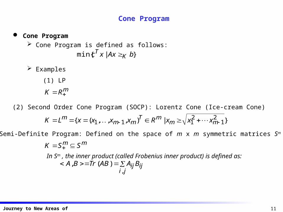
Cone Program
Cone Program Cone Program is defined as follows:
}|min{ bAxxc KT
Examples
}|),,,({ 21
2111 mm
mTmm
m xxxRxxxxLK
(2) Second Order Cone Program (SOCP): Lorentz Cone (Ice-cream Cone)
(1) LP
mRK
(3) Semi-Definite Program: Defined on the space of m x m symmetric matrices Sm
mm SSK In Sm , the inner product (called Frobenius inner product) is defined as:
ji
ijijBAABTrBA,
)(,

12Journey to New Areas of Optimization
Dual Cone Program
Dual Cone Program We want to derive dual cone program by using the same approach as LP. Since we use a generalized inequality, the problem is what numbers to be used.
bAx K bAx ,,
Note Inequalities are different!Conditions on λ?
0, bAx
Define dual cone K* as follows:
},0,|{* KaaEK Then we have:
*, KbAx K bAx ,,
So dual cone program can be defined as:
}0,*|,max{ *KcAb
Remark: A* is a conjugate operator defined as:
),(,*, EyRxxyAAxy n If we use orthogonal bases in both spaces, A* = AT.
13Journey to New Areas of Optimization
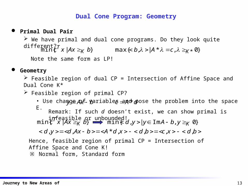
Dual Cone Program: Geometry
Primal Dual Pair We have primal and dual cone programs. Do they look quite different?
}|min{ bAxxc KT }0,*|,max{ *KcAb
Note the same form as LP!
Geometry Feasible region of dual CP = Intersection of Affine Space and Dual Cone K* Feasible region of primal CP?
• Use change of variables and pose the problem into the space E.
bAxy dAc *
}|min{ bAxxc KT }0,Im|,min{ KybAyyd
bdxcbdxdAbAxdyd ,,,,*,,
Remark: If such d doesn’t exist, we can show primal is infeasible or unbounded!
Hence, feasible region of primal CP = Intersection of Affine Space and Cone K! ※ Normal form, Standard form
14Journey to New Areas of Optimization
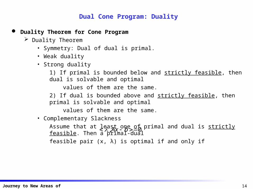
Dual Cone Program: Duality
Duality Theorem for Cone Program Duality Theorem
• Symmetry: Dual of dual is primal.
• Weak duality
• Strong duality
1) If primal is bounded below and strictly feasible, then dual is solvable and optimal
values of them are the same.
2) If dual is bounded above and strictly feasible, then primal is solvable and optimal
values of them are the same.
• Complementary Slackness
Assume that at least one of primal and dual is strictly feasible. Then a primal-dual
feasible pair (x, λ) is optimal if and only if
0, bAx

15Journey to New Areas of Optimization
Dual Cone Program: Duality (cont.)
Duality Theorem for Cone Program: Discussion Most of LP duality results hold, but we need strict feasibility…….. Why? Note that the feasible region of CP is the intersection of affine space and a cone. The cone in general is not polyhedral! So if there is very small change on the data (perturbation), the status can change!
You are now handling with non-polyhedral cones! Robustness is needed in practice. So strict feasibility requirement is not a problem.
16Journey to New Areas of Optimization
Cone Program: SOCP and SDP
First Observation on SOCP and SDP: They are self-dual! Dual cone of Lorentz cone is also Lorentz cone. Dual cone of Semi-definite cone is also Semi-definite cone.
From now on, we will study SOCP and SDP in detail.
17Journey to New Areas of Optimization
SOCP: Introduction
SOCP: Standard Form (Primal)
}|),,,({ 21
2111 mmmm
m xxxxxxxL
kmm LLK 1
},1,|min{}|min{ kibxAxcbAxxc iLiT
KT
im
iTi
iiii qp
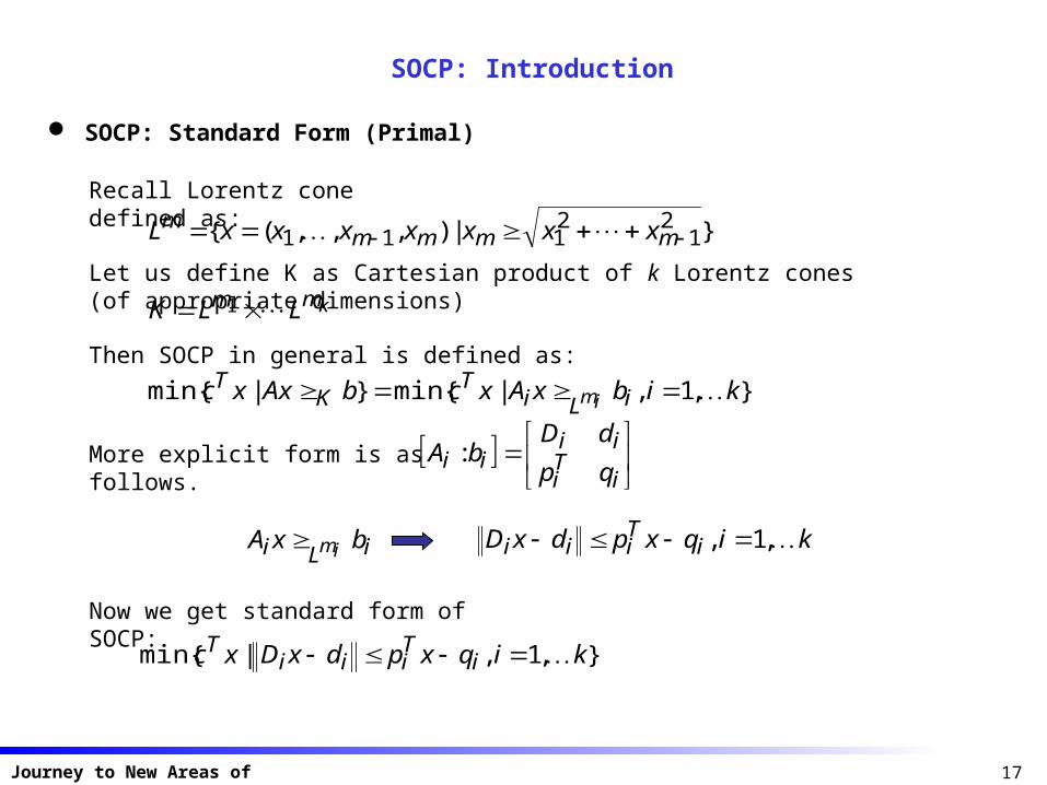
dDbA :
kiqxpdxD iTiii ,1,
},1,|min{ kiqxpdxDxc iTiii
T
Recall Lorentz cone defined as:
Let us define K as Cartesian product of k Lorentz cones (of appropriate dimensions)
Then SOCP in general is defined as:
More explicit form is as follows.
iLi bxA im
Now we get standard form of SOCP:

18Journey to New Areas of Optimization
SOCP: Introduction
SOCP: Some Observations
qxpdDx T
},1,|min{ kiqxpdxDxc iTiii
T SOCP:
Consider a single constraint:
• Note that the inequality is of quadratic form.• Easy to note that LP is a special case of SOCP (why?).• One more less easy observation: Quadratic program is a special case of SOCP.
Use Epigraph form (more on this later).• The left-hand side is a (square root of) sum of quadratic of linear function. Recall standard deviation from statistics!
Any idea on which problems to SOCP can be applied?
19Journey to New Areas of Optimization
SOCP: Introduction
SOCP: Standard From (Dual)
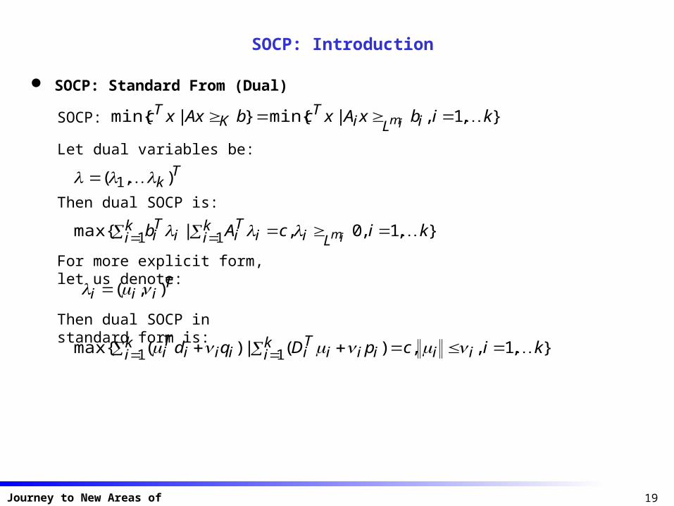
SOCP: },1,|min{}|min{ kibxAxcbAxxc iLiT
KT
im
Let dual variables be:
Tk ),( 1
Then dual SOCP is:
},1,0,|max{ 11 kicAb imLiki i
Ti
ki i
Ti
For more explicit form, let us denote:
Tiii ),(
Then dual SOCP in standard form is:
},1,,)(|)(max{ 11 kicpDqd iiki iii
Ti
ki iii
Ti
20Journey to New Areas of Optimization
SOCP: Expressive Power
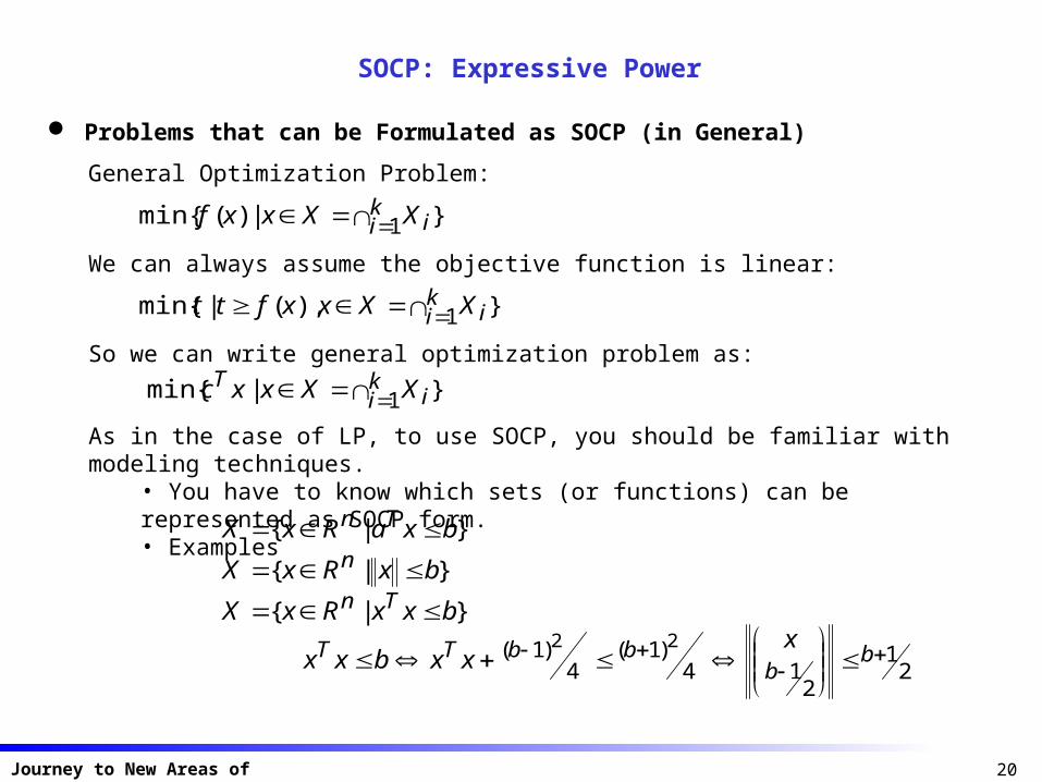
Problems that can be Formulated as SOCP (in General)
General Optimization Problem:
}|)(min{ 1ki iXXxxf
We can always assume the objective function is linear:
}),(|min{ 1ki iXXxxftt
So we can write general optimization problem as:
}|min{ 1ki i
T XXxxc
As in the case of LP, to use SOCP, you should be familiar with modeling techniques.• You have to know which sets (or functions) can be represented as SOCP form.• Examples
}|{ bxaRxX Tn
}|{ bxRxX n
}|{ bxxRxX Tn
21
214
)1(4
)1( 22
b
bbbTT x
xxbxx

21Journey to New Areas of Optimization
SOCP: Expressive Power
Problems that can be Formulated as SOCP (cont.)
Many sets can be represented in SOCP form.Usually, you start with basic sets (e.g., sets in the previous slide) and take some operations on the sets that preserve the representability.
• For example, affine image of a set is also SOCP representable.
Not easy, but if you become familiar, very useful.
22Journey to New Areas of Optimization
SOCP: Robust LP
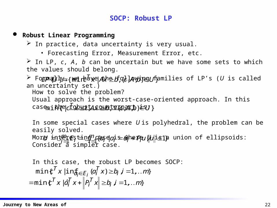
Robust Linear Programming In practice, data uncertainty is very usual.
• Forecasting Error, Measurement Error, etc. In LP, c, A, b can be uncertain but we have some sets to which the values should belong. Formally, we have the following families of LP’s (U is called an uncertainty set.)
}),,(,|{min)( UbAcbAxxcULP T
How to solve the problem?Usual approach is the worst-case-oriented approach. In this case, the robust counterpart is:
}),,(,,|min{ UbAcbAxtxct T
In some special cases where U is polyhedral, the problem can be easily solved.More interesting case is where U is a union of ellipsoids: Consider a simpler case.
mi iiii
mi i uuPaaaEU 11 }1,ˆ|{
In this case, the robust LP becomes SOCP:
},1,)(inf|min{ mibxaxc iTiEa
Tii
},1,ˆ|min{ mibxPxaxc iTi
Ti
T

23Journey to New Areas of Optimization
SOCP: Stochastic LP
Stochastic Linear Programming Chance-Constrained Programming
},,1,)Pr(|min{ mibxaxc iTi
T
Let us assume (multivariate) Gaussian distribution:
),ˆ(~ iii VaNa
Then the problem becomes:
},,1,)(ˆ|min{ 2/11 mibxVxaxc iiTi
T where is a Gaussian CDF.
24Journey to New Areas of Optimization
SOCP: Concluding Remarks
Applications of SOCP Usual sources of applications of SOCP come from
• Engineering Design Problems: Mechanics, etc
• Robust Linear Model: Finance, Inventory Management, SCM
For OR people, SOCP can be viewed as a tool to handle data uncertainty on linear model.
Research Topics on SOCP Mainly modeling issues.
• What applications can be modeled by SOCP ?
For e.g., Goldfarb and Iyenger (2003) showed that robust portfolio optimization problem
can be formulated as SOCP.
• Potentially huge applications in other areas such as problems with demand uncertainty. Theoretical and Algorithmic issues
25Journey to New Areas of Optimization
SDP: Introduction
SDP: Standard Form (Primal)
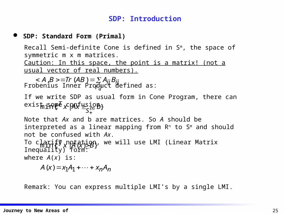
Recall Semi-definite Cone is defined in Sm, the space of symmetric m x m matrices.Caution: In this space, the point is a matrix! (not a usual vector of real numbers).
Frobenius Inner Product defined as:
ji
ijijBAABTrBA,
)(,
If we write SDP as usual form in Cone Program, there can exist some confusion.
}|min{ bAxxc mST
Note that Ax and b are matrices. So A should be interpreted as a linear mapping from Rn to Sm and should not be confused with Ax. To clarify notation, we will use LMI (Linear Matrix Inequality) form:
})(|min{ BxAxcT
where A(x) is:
nn AxAxxA 11)(
Remark: You can express multiple LMI’s by a single LMI.
26Journey to New Areas of Optimization
SDP: Introduction
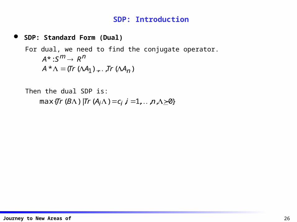
SDP: Standard Form (Dual)
For dual, we need to find the conjugate operator. nm RSA :*
))(,),((* 1 nATrATrA
Then the dual SDP is:
}0,,,1,)(|)(max{ nicATrBTr ii

27Journey to New Areas of Optimization
SDP: Modeling Power
SDP: Expressive Power Many important applications of SDP uses the fact that functions of eigenvalues of a matrix
can be represented as SDP. Simple example: The largest eigenvalue
Note the above is the subset of m x m symmetric matrices with the largest eigenvalue t. You can express the set as LMI as follows:
})(|{ max tXSX m
}0|{ XtISX mm
Other examples- Sum of k largest eigenvalues- Spectral norm of a symmetric m x m matrix X- Negative powers of determinants, e.g., 1/Det(X)
Also you can show SOCP is a special case of SDP. Usual engineering application of SDP involves the stability of linear system.
• Important application contains Liapunov Stability Theory for uncertain linear system.

28Journey to New Areas of Optimization
SDP: Combinatorial Optimization Application
General SDP Relaxation Scheme: Shor’s Relaxation We can formulate (0,1) IP problem as the form:
0000 2)(min cxbxAxxf TT
micxbxAxxf iTii
Ti ,,1,02)(
Note that any Boolean variable can be represented as: .02 jj xx
General relaxation scheme comes from Lagrange relaxation constructed as: .
)()(2)()( cxbxAxxf T where . i
mi i AAA 10)(
Note from the above construction, if .nRxxf ,0)(
Then ζ is a lower bound on the original problem. .
29Journey to New Areas of Optimization
SDP: Combinatorial Optimization Application
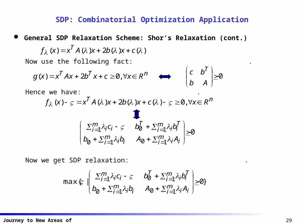
General SDP Relaxation Scheme: Shor’s Relaxation (cont.)
)()(2)()( cxbxAxxf T Now use the following fact: .
nTT RxcxbAxxxg ,02)( 0
Ab
bc T
Hence we have: .nT RxcxbxAxxf ,0)()(2)()(
01010
101
mi ii
mi ii
mi
Tii
Tmi ii
AAbb
bbc
Now we get SDP relaxation: .
}0|max{1010
101
mi ii
mi ii
mi
Tii
Tmi ii
AAbb
bbc
30Journey to New Areas of Optimization
SDP: Combinatorial Optimization Application
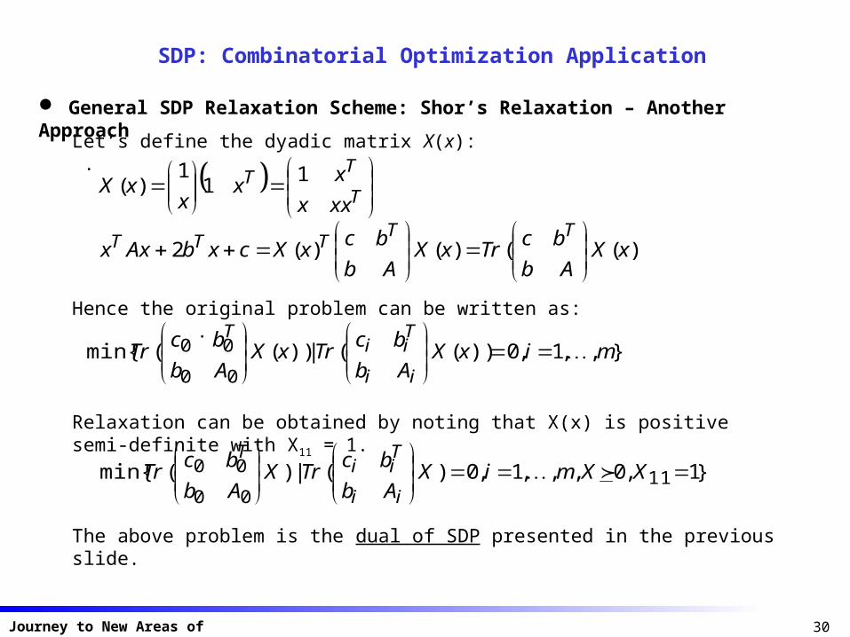
General SDP Relaxation Scheme: Shor’s Relaxation – Another Approach
Let’s define the dyadic matrix X(x): .
T
TT
xxx
xx
xxX
11
1)(
))(()()(2 xXAb
bcTrxX
Ab
bcxXcxbAxx
TTTTT
Hence the original problem can be written as: .
},,1,0))((|))((min{00
00 mixXAb
bcTrxX
Ab
bcTr
ii
Tii
T
Relaxation can be obtained by noting that X(x) is positive semi-definite with X11 = 1.
}1,0,,,1,0)(|)(min{ 1100
00
XXmiX
Ab
bcTrX
Ab
bcTr
ii
Tii
T
The above problem is the dual of SDP presented in the previous slide.
31Journey to New Areas of Optimization
SDP: Combinatorial Optimization Application
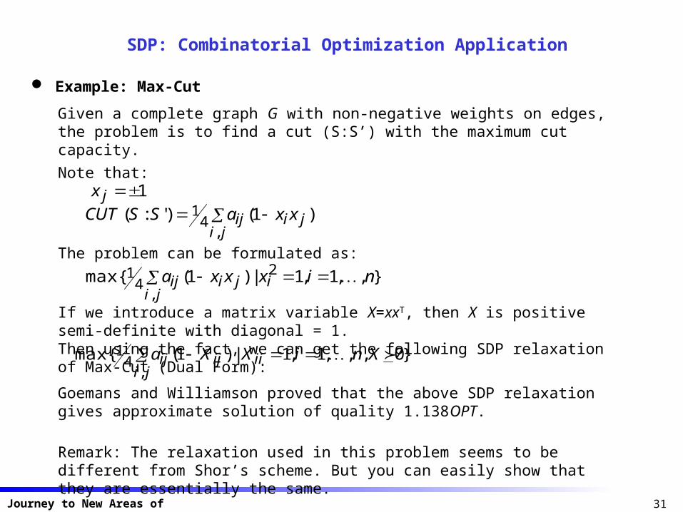
Example: Max-Cut
Given a complete graph G with non-negative weights on edges, the problem is to find a cut (S:S’) with the maximum cut capacity.
Note that:1jx
ji
jiij xxaSSCUT,
41 )1()':(
The problem can be formulated as:
},,1,1|)1(max{ 2
,4
1 nixxxa iji
jiij
If we introduce a matrix variable X=xxT, then X is positive semi-definite with diagonal = 1.Then using the fact, we can get the following SDP relaxation of Max-Cut (Dual Form):
}0,,,1,1|)1(max{,
41 XniXXa ii
jiijij
Goemans and Williamson proved that the above SDP relaxation gives approximate solution of quality 1.138OPT.
Remark: The relaxation used in this problem seems to be different from Shor’s scheme. But you can easily show that they are essentially the same.
32Journey to New Areas of Optimization
SDP: Concluding Remarks
SDP: General Advice SDP is a powerful tool to model many engineering design problems, especially those involving
linear system design. The major difficulty when studying SDP comes from the fact that you should deal with matrix
variables and extensive knowledge on matrix analysis is necessary. However, if you master SDP, there will be very interesting problems waiting for you!
Research Topics As in the case of SOCP, most of the research focuses on the applicability of SDP. Besides engineering applications, combinatorial optimization is one of the most promising
area of application. For e.g., comparing the quality of relaxation using SDP with others. In finance applications, asset pricing problems and robust portfolio optimization problems
can be handled with SDP, e.g., El Ghaoui (1999) when only partial information on the
covariance matrix is given. Of particular interest, the moment problem is to deal with uncertainty when only partial
moment information on the random variables is given. This model is robust in that it does not
assume any particular distribution function. Applications include finance, combinatorial
optimization (probabilistic analysis of heuristics) and others, see Bertsimas (2000).

33Journey to New Areas of Optimization
Algorithms for Cone Program
Interior Point Algorithm in General Newton Method for Unconstrained Convex Optimization
• Use second-order (quadratic) approximation
• Two phases
1) Damped Phase: When current iterate is far from optimal Linear Convergence
2) Pure Newton Phase: When current iterate is near optimal Quadratic Convergence Generic Scheme
• Use barrier function to represent the interior of feasible region
• Convert the problem into unconstrained one by summing the objective and barrier
functions
• Sequentially solve the problem by Newton method.

34Journey to New Areas of Optimization
Algorithms for Cone Program
Interior Point Algorithm in General Classical Interior Penalty Scheme
Given an optimization problem (recall we can assume the objective is linear):
}|min{ XxxcT
Choose a barrier function (interior penalty function) F(x) satisfying:
ixFXbdxxXx iii ,)()(,int
Transform the problem into optimization of parametric family of functions:
RXxFxtcxF Tt int:)()(min
Under some mild conditions, we can show that:1) Ft(x) has its minimum in the interior of X and the minimizer x*(t) is unique.2) The central path x*(t) is smooth curve and as t , the point approaches an optimal solution of the original problem.
The method: Solve an initial problem and get x*(0)1) Increase t a bit (Small increase of t will make the current iterate x*(t i) close to x*(ti+1)).2) Solve new problem to get a solution x*(ti+1).
35Journey to New Areas of Optimization
Algorithms for Cone Program
Problems in Classical Interior Penalty Scheme The method is straightforward and very intuitive, but There is too much freedom (ambiguity) including
• How to update t.
• How to check whether the current iterate is sufficiently close to central path
• How to ensure fast convergence of Newton method The result is: We don’t know when the algorithm terminates…….
Cure: Self-Concordant Barrier Functions There exists good barrier functions with property called self-concordance. With self-concordant barrier functions, we can
• Specify how close the current iterate to central path.
• Updating t is quite simple: Use self-concordance parameter.
• Show the step needed to obtain ε-optimal solution is polynomial. The result is: We can make a polynomial time algorithm to obtain ε-optimal solution.
Remark: Self-concordance barrier function is three times continuously differentiable and
satisfies two conditions relating first and second derivatives, and second and 3 rd derivatives.

36Journey to New Areas of Optimization
Algorithms for Cone Program
Self-Concordance Barrier Function for SOCP and SDP
)ln()( 21
21
2 kkk xxxxL
SOCP case:
)(ln)( XDetXSk SDP case:
Remark 1: For these functions, the calculation of gradient and Hessian is very simple.Remark 2: The algorithm is called a central path following method.
37Journey to New Areas of Optimization
Cone Program: Concluding Remarks
Cone Program as a Tool of Problem Solving Now, CP can be treated as a tool.
• For SOCP, MOSEK can solve very large problem instances very efficiently.
• For SDP, some refinement is needed, but problems with around 2,000 variables can be
solved in a reasonable time. To fully make use of SOCP and SDP,
• Much work remains in the modeling issues.
• Study the full expressive power of SOCP and SDP
Research Suggestions Analyze the expressive power of SOCP and SDP in various fields of applications. Research on SDP relaxations for Discrete Optimization Problems (and approximation scheme) Study other class of useful cone programs.
38Journey to New Areas of Optimization
Journey II
Robust Optimization

39Journey to New Areas of Optimization
Robust Optimization: Introduction
Uncertainty We live in a dynamic and uncertain world!
• Speed of change accelerates itself!
• Even worse, the cycle of change gets shorter and shorter…. But anyway, you plan and act now and see the result in the future. How can we handle uncertainty?
Sources of Uncertainty Forecasting Error
• Future demand/price/interest rate/weather/etc….
• Any forecasting model has an error term.
• Even worse for long term forecasting Measurement Error
• In engineering applications, though there would exist accurate value for an object to be
measured, error is very usual.
• Precision of measurement, Human error, Computer error, etc
40Journey to New Areas of Optimization
Robust Optimization: Introduction
Modeling Uncertainty Of course, the first way of modeling uncertainty is to use probability distributions.
• E.g., probability distribution for future demand
• Two main difficulties
1) Very difficult to estimate the probability distribution
2) Very difficult to solve the optimization problem (stochastic program)
• One more less apparent drawback
The probability distribution itself can be very sensitive to forecasting error.
To overcome the problem, non-parametric approach (usually based on order statistics) can be used, but the optimization becomes more difficult.
Uncertainty Set
• Though we cannot exactly specify the value of a parameter, it is reasonably easy to define
a set in which the parameter takes its value.
E.g., You can define an interval for next year’s demand for oil.
• Using properly defined uncertainty set makes optimization a tractable one.
• One major drawback is that the solution can be too conservative since we don’t assume
any probability on the data in the set. (Can take a solution that reflects very rare and worst
case)
41Journey to New Areas of Optimization
Robust Optimization: Introduction
Robust Optimization Uncertainty Set Approach
• Rather than assuming any particular pdf, use uncertainty set to model data uncertainty. Worst-case Oriented Approach
• The solution should be feasible for all possible cases that come from the uncertainty set.
• Maximize/Minimize the worst-case revenue/cost. Usually, there is a method to control the conservatism of the solution, so some possibility of
infeasibility can be permitted.
Main Topics in Robust Optimization Uncertainty Set: Good uncertainty set has the following properties.
• It should be able to model the data uncertainty effectively.
• The optimization problem (called robust counterpart) should be tractable. So the major issue in RO is to develop effective uncertainty set model where its robust
counterpart should be tractable.

42Journey to New Areas of Optimization
Robust Optimization: Uncertainty Set
Popular Uncertainty Set Models Ellipsoid
• To model multiple parameter values.
• Defined by nominal values of parameters and a symmetric positive definite matrix
}1|{}1)()(|{ 2/11 uuPaaaPaaaE T
Remark 1: Ellipsoid uncertainty set is very useful to model forecasting errors from regression.Remark 2: LP with ellipsoidal uncertainty set becomes SOCP.
Interval Set
• To model independent parameter values.
• Defined by a nominal value with its maximum possible deviation
]ˆ,ˆ[ aaaaU
Remark 1: Interval uncertainty set is very easy to estimate. But also independency may matter.Remark 2: Linear model with interval uncertainty set will be linear model (more on this later)Remark 3: Generalization to polyhedral uncertainty set is possible.
43Journey to New Areas of Optimization
Bertsimas and Sim Model
Bertsimas and Sim Model Uses Interval Uncertainty Set
• Robust counterpart of linear model remains linear.
LP, IP: Broad applicability
• Robust counterpart of discrete optimization problem with polynomial time solvability can
also be solved in a polynomial time. Method to control conservatism: The probability of constraint violation can be controlled by a
single parameter.
44Journey to New Areas of Optimization
Bertsimas and Sim Model
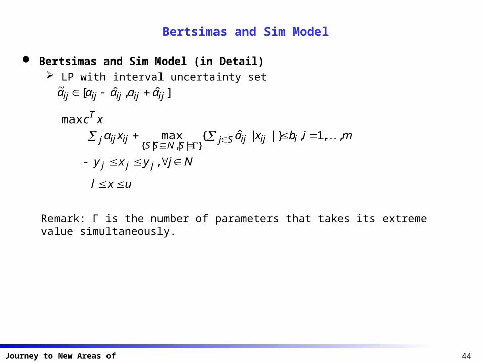
Bertsimas and Sim Model (in Detail) LP with interval uncertainty set
]ˆ,ˆ[~ijijijijij aaaaa
xcTmax
mibxaxa Sj iijijSNSS
j ijij ,,1,|}|ˆ{max}||,|{
Njyxy jjj ,
uxl
Remark: Γ is the number of parameters that takes its extreme value simultaneously.

45Journey to New Areas of Optimization
Bertsimas and Sim Model
Bertsimas and Sim Model (in Detail)
Note the following fact (LP duality)
}10,||ˆ|ˆmax{ ijSj Nj ijijijij zzzxa
}0,0|,ˆ|ˆ|min{ Nj iijijijijiiij zpxapzzp
So the problem becomes:
xcTmax Nj iijiNj jij mibpzxa ,,1,
jiyapz jijiji ,,ˆ
jyxy jjj ,
uxl jizyp ijij ,,0,,
Remark 1: Still LP with moderately larger sizeRemark 2: In case of IP, still IP with moderately larger sizeRemark 3: Γ can be chosen to reflect the probability of constraint violation.

46Journey to New Areas of Optimization
Example of Robust Optimization Application
Robust Portfolio Selection (Goldfarb and Iyenger 2003)
Use multi-factor model for asset return:
fVr T
Uncertainty Set• Mean return: Interval (min and max is given.)• Columns of factor loading matrix: Ellipsoid• Variance of residual: Interval
Result: Robust counterpart is SOCP. (Note the original portfolio optimization problem is a quadratic programming model.)

47Journey to New Areas of Optimization
Robust Optimization: Concluding Remarks
Robust Optimization as a Tractable Method to Handle Data Uncertainty Much more practical applicability than stochastic programming approach The key to success is how to model U:
• Effective to capture the uncertainty and also easy to define
• Tractable robust counterpart e.g., LP, IP, SOCP, SDP
Research Suggestions Research on Uncertainty Set Modeling
• For example, to which uncertainty sets, SOCP can handle?
• Develop specific uncertainty set modeling for particular field of application Extension of IP
• Apply Bertsimas and Sim framework to various IP models. Theoretical Issues
• Linking Stochastic Programming (especially, chance-constrained program) and RO

48Journey to New Areas of Optimization
Discussion and Q&A
Top Related