


Languages
Pages
Legal

Job Location, Neighborhood Change, and Gentrification
Jed Kolko Public Policy Institute of California
June 2009
ABSTRACT
This paper assesses the contribution of employment location to neighborhood
change and to gentrification. At the tract level, average household income change is positively correlated both with the change in average pay for nearby jobs and with the start-year average pay for nearby jobs. The relationship between employment location and neighborhood change is stronger for tracts closer to downtown and for tracts in larger metropolitan areas. Change in job pay helps explain metropolitan gentrification within 2 miles of the CBD.
The analysis combines Census tract household data for 1990-2000 from the Neighborhood Change Database and zip-code-level employment data for 1992-2000 from the National Establishment Time-Series database. I develop an algorithm for identifying changes in zip codes over time and for matching non-standard zip codes to Census tracts. Because causality between employment location and household location could run in both directions, I instrument for the tract-level change in average job pay with national-level industry growth and average pay. Contact information: [email protected]. Thanks to Jan Brueckner, Shihe Fu, Edward Glaeser, Claudia Goldin, Rucker Johnson, Larry Katz, Jeffrey Lin, Stuart Rosenthal, Tara Watson, anonymous referees, and APPAM conference participants for helpful feedback, and thanks to Davin Reed for research assistance.

1
In most American metropolitan areas, average household income rises with
distance from the central business district (CBD). Over the last two decades, though,
household incomes near the CBD have grown, relative to metropolitan average income,
for larger metropolitan areas. Gentrification refers to this increase in relative income in
downtown neighborhoods. Because gentrification represents a deviation from the
traditional income-distance relationship in American cities, understanding gentrification
can shed light on the causes of neighborhood change in general.
In this paper, I test whether changes in employment location and composition –
summarized using average job pay -- affect average neighborhood income; to handle
the endogeneity of employment location and composition with respect to household
location, I instrument for tract-level employment changes using national-level
employment changes by industry. I generate average neighborhood pay per job from
employment counts by zipcode and industry and average industry pay nationally; I
combine these measures of average neighborhood pay per job with data on average
household income by Census tract.
Both the 1992 level and 1992-2000 change in average neighborhood job pay
have a positive, statistically significant effect on 1990-2000 change in tract-average
household income. The positive effect of the level of neighborhood job pay on average
neighborhood income suggests that tastes or commuting costs changed in a way that
caused workers to want to live closer to their jobs; the positive effect of the change in
neighborhood job pay on average neighborhood income suggests that, to some extent,
households follow jobs. The metropolitan-area-level analysis shows that changes in
2
average downtown pay have a positive effect on changes in average incomes within 2
miles of the CBD, relative to metropolitan-wide changes in pay and income, though this
result does not hold for changes within 5 miles of the CBD. Changes in employment
location, therefore, contributed to neighborhood change and gentrification in the
1990’s.
EXISTING RESEARCH
The primary contribution of this paper is to take employment location into
account and to show that employment location affects neighborhood change. Existing
research on neighborhood change and gentrification often relies on the monocentric
city model and dynamic housing filtering models, which assume all employment is at the
CBD, or dynamic tipping models, which do not incorporate employment. Dynamics in
these models arise from changing household tastes, changing commuting costs, and real
estate depreciation and re-investment. Accordingly, the literature has explained
gentrification and neighborhood change using factors like the age of the housing stock,
characteristics of one’s neighbors, and transportation availability, but not factors like
changes in employment location or composition.
In the monocentric city model, households maximize utility over commuting
costs, which are lower nearer the city center, and housing costs, which are higher nearer
the city center.1 All employment is assumed to be at the city center, from which
commuting costs rise with distance. Theoretically, the relationship between income and
1 Brueckner (1987) presents the model.

3
proximity to the city center is ambiguous and depends on the income elasticities of
housing demand and commuting costs (Muth, 1969; Wheaton, 1977). Empirically,
income rises with distance from city center, though the relationship is more U-shaped in
older cities and closer to monotonically increasing in Sunbelt cities; Glaeser, Kahn, and
Rappaport (2007) show that the greater availability of public transit in central cities
accounts for more of the income-distance relationship than other factors like the
income elasticity of demand for housing. Gentrification can arise if income elasticities of
commuting costs or housing demand change, which could arise from a shift in tastes for
housing, changes in transportation technology, or changes in the composition of
households with different elasticities. High-income groups with lower demand for
housing include young childless couples (Kern, 1984; Myers, 1990) and gay people
(Knopp, 1997; Fu, 2006; Black et al, 2002); their growth could contribute to
gentrification, especially if they also have higher demand for centrally-located
amenities. General increasing demand for urban consumption opportunities and other
amenities could also lead to gentrification and inner-city growth (Glaeser, Kolko, and
Saiz, 2001). The development of new transit centers or the increasing demand for
proximity to existing transit centers can lead to gentrification (Lin, 2002, and Kahn,
2007). The monocentric model, therefore, yields predictions that changes in
demographics, tastes, or commuting costs could contribute to gentrification.
Dynamic housing models also can predict gentrification and neighborhood
change. Filtering models assume a monocentric city with all employment in the center.
The oldest housing is initially nearest the city center, and housing age (in the absence of

4
renovation) declines with distance from the center. Housing units deteriorate over time
and are occupied by successively poorer households while new housing is constructed at
the edge of the city, so income rises with distance from the city center (Muth, 1973).
Rehabilitation of deteriorated housing stock can constitute reverse filtering, or “filtering
up,” when deterioration is sufficient to warrant the rehabilitation cost (Bond and
Coulson, 1989; Bourne, 1981). Empirically, older buildings are indeed more likely to
gentrify (Helms, 2003). Brueckner and Rosenthal (2009) show that, controlling for age of
neighborhood housing stock, neighborhood income declines with distance from the city
center, and predict that the redevelopment of older housing stock near city centers will
lead to further gentrification.
Tipping models, often used in the racial segregation literature, provide additional
possible reasons for gentrification (Schelling 1978; Bailey, 1959). In these models,
household decisions depend on their neighbors’ characteristics: these externalities or
spillovers might occur between households in a neighborhood or between proximate
neighborhoods. Empirically, changes in neighborhood income or racial composition are
affected by adjacent neighborhood characteristics (Aaronson, 2001; Galster, 1990) as
well as own-neighborhood initial conditions (Galster et al., 2003; Rosenthal, 2008; and
many others).
The above studies do not consider employment growth or changes in
employment composition as explanations for gentrification. This question of whether
people follow jobs is central, however, to the related literature on spatial mismatch.
Ihlanfeldt and Sjoquist (1998) define the spatial mismatch hypothesis as fewer jobs per
5
worker in black neighborhoods relative to white neighborhoods; spatial mismatch is
caused by employment suburbanization combined with limited black residential
mobility and high commuting costs, resulting in worse labor market outcomes for
blacks. Their review of the literature generally supports the spatial mismatch
hypothesis, which implies that blacks (or other disadvantaged workers) do not follow
jobs fully. But even if people don’t follow jobs fully, employment location could affect
neighborhood change so long as people follow jobs to some extent. Martin (2001) finds
that black population shifts offset 57% of the effect of employment shifts, which
supports the spatial mismatch hypothesis yet is evidence that people follow jobs
somewhat. Since spatial mismatch focuses on the movement of blacks or other
disadvantaged groups with tighter constraints on mobility, the responsiveness of
residential location to employment shifts for the overall population might be greater
than estimated in the spatial mismatch literature.
A challenge in the spatial mismatch literature is the simultaneous determination
of residential location and employment location. Research has long demonstrated that
not only do people follow jobs, but jobs follow people (Steinnes, 1977; Cooke, 1978;
Steinnes, 1982; Boarnet, 1994). In their literature review, Ihlanfeldt and Sjoquist (1998)
say that the most common approach to handling this simultaneity in the spatial
mismatch literature is to focus on youth, assuming that their residential location is
exogenously determined (from the youths’ perspective) by their parents or guardians.
An alternative approach is to instrument for levels or changes in employment location
using shift-share measures. Weinberg (2004) instruments for central-city share of

6
metropolitan-area employment using metropolitan-area industry composition and
national shares of central-city employment by industry. He finds that, in cross-section,
higher central-city labor demand raises wages for central-city residents and the
likelihood of employment for blacks. Dworak-Fisher (2004) instruments for regional
employment growth using regional industry composition and changes in national
industry growth.2 He finds that average wages and likelihood of employment rise when
employment demand rises, at the county-group level, especially for demographic
groups with less education or less experience.
This paper advances research on gentrification and neighborhood change by
considering job growth and changes in job composition. Furthermore, it advances the
spatial mismatch literature by looking at job location and residential characteristics at
the Census tract level, rather than at the metropolitan area or multi-county levels, as
Weinberg (2004) and Dworak-Fisher (2004) do.3
DATA AND DESCRIPTIVES
Average household income
Data for this paper come from two sources: household data from the
Neighborhood Change Database (NCDB), and employment data from the National
Establishment Time-Series (NETS).
2 Regions, in his paper, are “county groups” of one or more counties within a metropolitan area. Each metropolitan area contains at least two county groups. 3 Most of the gentrification and neighborhood change research cited above uses Census tracts as the unit of observation.

7
The NCDB compiles tract-level data from the 1970, 1980, 1990, and 2000
decennial Censuses, recalculated using a consistent definition of tract boundaries in
order to facilitate comparison over time. The NCDB covers all Census tracts in the U.S.
The NCDB was originally created by the Urban Institute and is now distributed by
Geolytics, Inc.4 My measure of neighborhood change at the tract level is growth in tract
average household income.
Gentrification in a metropolitan area refers to an increase over time in
household income in tracts near the CBD relative to the metropolitan average.5 To
identify the tract that best represents a metropolitan area’s CBD, I use the Census’s
1982 Geographic Reference Manual list of CBD’s.6 For metropolitan areas with multiple
CBD tracts identified in 1982 by the Census, I chose the tract with the highest
employment density in the immediate area.7 For metropolitan areas where the Census
identified no CBD tract, I use the coordinates of City Hall of the largest city in the
metropolitan area, as given by Google Maps. For each tract, I calculate the distance
from its centroid to the centroid of the metropolitan area’s CBD tract.8
4 Documentation is available at http://www.geolytics.com/Pages/NCDB/NCDB_Variables/NCDBDataUsersGuide.pdf . 5 Hammel and Wyly (1996) consider several quantitative indicators of gentrification, such as income, housing variables, and other economic and demographic data, and they determine that tract income change is the quantitative measure that best fits field-survey classifications of gentrifying neighborhoods. 6 The 1982 Economic Census identified the central-business-district (CBD) census tracts for all metropolitan areas by surveying officials in each city. CBD tracts were published in the 1982 Geographic Reference Manual, available at http://www.census.gov/geo/tiger/cbdct.pdf. CBD census tracts were not identified in any other year. 7 Specifically, I used the average employment density of the nearest five zipcodes, weighted by the inverse of distance between zip codes’ centroids and the CBD tract centroid. 8 Tract centroids for CBD tracts were generated using the MABLE/Geocorr engine at http://mcdc2.missouri.edu/websas/geocorr2k.html .
8
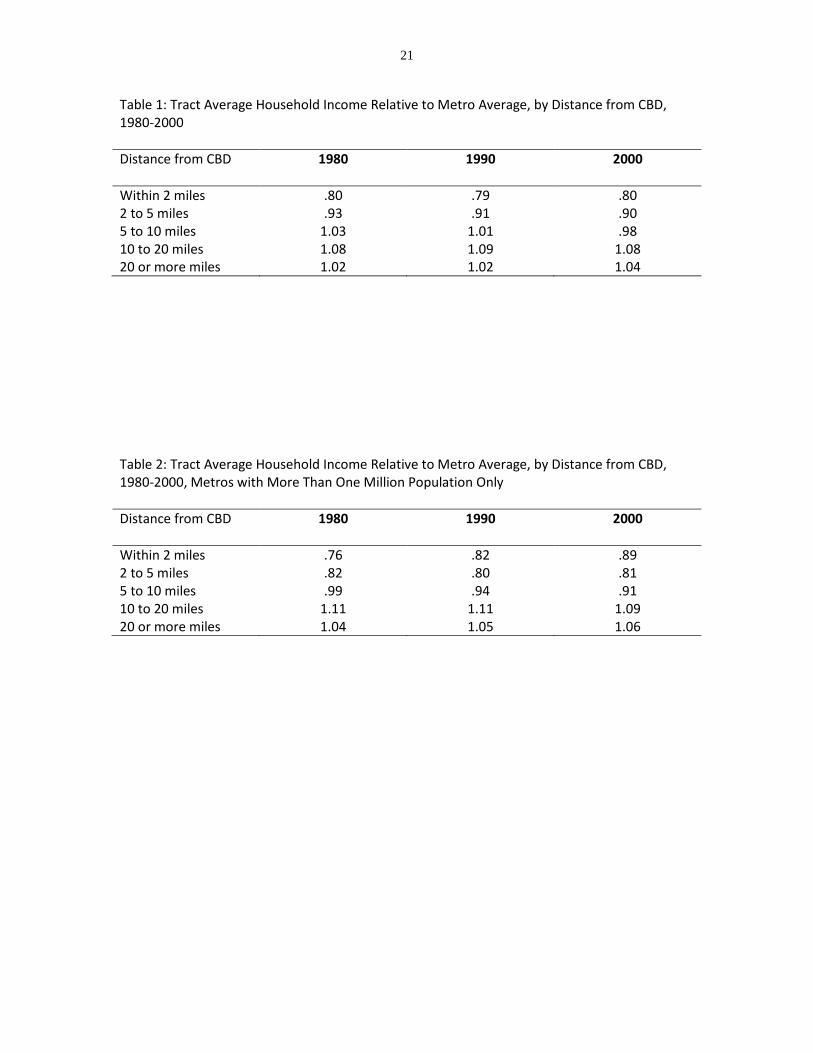
Tract average household income generally increases with distance from the CBD,
as shown in Table 1. In 2000, the ratio of average household income within 2 miles of
the CBD relative to the metropolitan area average was .80, rising with distance to 1.08
at 10-20 miles from the CBD, and falling a bit to 1.04 beyond 20 miles from the CBD.
Table 1 shows no change in relative household income over the period within 2 miles for
either the 1980’s or the 1990’s, and a slight decline in the ring 2-5 miles from the CBD.
For metropolitan areas with one million population or more (in 2000), relative
household income within 2 miles of the CBD rose from .76 in 1980 to .82 in 1990 and to
.89 in 2000. For these larger metropolitan areas, relative tract income changed little in
the 2-5 mile ring and declined in the 5-10 mile ring. Gentrification, therefore, appears to
be a general trend only for the area closest to downtown and only for larger
metropolitan areas. Of course, average household income can rise in a downtown tract
even if that tract’s metropolitan area is not gentrifying: within metropolitan areas, even
at a given distance from the CBD, tract income growth can vary.
Average job pay
Calculating average tract job pay, and the relationship between job pay and
distance from CBD, is more complicated. I rely on the National Establishment Time-
Series (NETS) database, a national, longitudinal file of the universe of business
establishments created by Walls & Associates using establishment-level data from Dun
& Bradstreet, a leading provider of business credit information and credit reports. The
NETS database does not contain a rich set of information about each establishment, but
9
it does include the business name, a unique D&B establishment identifier (the DUNS
number), the establishment’s street address, both SIC and NAICS industrial codes in
each year, the identifier of the firm’s headquarters, and employment in each year. My
extract of the NETS covers the entire U.S. over the period 1992-2006.9
I estimate tract level employment by industry using the establishment’s zip code
provided in the NETS and convert zip code employment to Census tracts. The
MABLE/Geocorr engine provides a correspondence between Zip Code Tabulation Areas
(ZCTA’s) and Census tracts in 2000. ZCTA’s are a close approximation to zip codes; like
Census tracts, ZCTA’s represent geographic areas with boundaries that can be mapped
and overlaid with other geographies.10 The NETS reports zip code for each business
establishment, and while most zip codes have a corresponding ZCTA, many do not, for
two reasons. First, many zip codes are unique to a building or large institution, or they
refer to P.O. boxes instead of a physical business location; these non-standard zip codes
typically have no residential addresses and represent a geographic point (or, in the case
of P.O. boxes, only a virtual location) rather than a geographic area (or “polygon” in GIS-
speak). Non-standard zip codes typically have no ZCTA equivalent. Second, zip codes
regularly change, and the U.S. Postal Service does not make public a comprehensive list
of historical zip code changes; ZCTA’s are defined decennially and are not updated every
time the U.S. Postal Service changes a zip code. These are two important reasons why
9 For more information on the NETS, including assessment of the data quality, see Kolko and Neumark (2007), Appendix A. Unfortunately NETS data are not available for earlier years, so I cannot use NETS data that line up exactly with the 1990 Census data. 10 See http://www.census.gov/geo/ZCTA/zcta.html for the Census’s explanation of ZCTA’s and http://mcdc2.missouri.edu/webrepts/geography/ZIP.resources.html for a detailed explanation of numerous issues affecting zip-code-level analysis.
10
some businesses in the NETS have zip codes that lack corresponding ZCTA’s and
therefore cannot be straightforwardly converted to Census tracts.
I handle these two zip code challenges in the following ways. First, to assign non-
standard zip codes to ZCTA’s, we use the ESRI StreetMaps in ArcGIS to overlay a map of
standard zip-code polygons, which usually correspond to ZCTA’s, with a map of the non-
standard zip-code points, thereby assigning many of the non-standard zip codes to the
standard zip code containing it. For non-standard zip codes that could not be mapped
this way, I associate each non-standard zip code for which geographic coordinates were
available to the ZCTA with the closest centroid. Second, to deal with zip code changes
over time, I take advantage of the NETS database’s longitudinal structure to infer zip
code changes. I look at all establishments that exist in both 1992 and 2000. If the
majority of establishments in a 1992 zip code have a different zip code in 2000 (or vice
versa), I assume that the zip code boundary or number changed. Zip code boundary
changes, of course, are not the only reason why an establishment’s zip code could
change: the establishment could have relocated to a new zip code. However, it is highly
unlikely that the majority of establishments in a given zip code would all relocate
together to a single different zip code. Using this method, I create a file showing major
zip code changes between 1992 and 2000 and am able to assign businesses that had a
1992 zip code that ceased to exist to the correct zip code in 2000, and therefore to a
2000 ZCTA.11 Roughly 5% of NETS employment in 1992 and 2000 was located in zip
11 Two examples of major changes are the renumbering of many 021XX zip codes to 024XX in Boston’s western suburbs, and of many 926XX zip codes to 928XX zip codes in Orange County, California.

11
codes that did not correspond to a 2000 ZCTA and was converted to a 2000 ZCTA using
the above methods.12
After converting 1992 zip codes and 2000 zip codes to 2000 ZCTA’s, I estimate
tract-level employment by apportioning ZCTA employment to tracts in proportion to the
share of ZCTA households in each tract (from the Mable/GEOCORR engine). To estimate
the levels and change in average job pay, I use national average pay by 3-digit NAICS
industry, reported in the Quarterly Census of Earnings and Wages, for 1992 and 2000.
Aggregate pay in a tract is equal to the sum, across 3-digit industries, of tract
employment in an industry multiplied by national average pay in that industry; tract
average job pay equals tract aggregate pay divided by tract employment.13
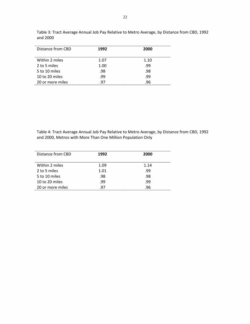
Tract average job pay – unlike tract average household income – declines with
distance from the CBD. The ratio of tract average pay in the 2-mile circle around the CBD
relative to the metropolitan area was 1.07 in 1992 and 1.10 in 2000, as shown in Table
3. Beyond 2 miles from the CBD, tract average job pay is fairly constant. In the largest
metropolitan areas, tract average pay in the 2-mile circle around the CBD is even higher
relative to the metro average – 1.09 in 1992 and 1.14 in 2000. The 1992 industry-level
correlation between distance of the average job from the CBD and average pay is -.33 (-
.30 when weighted by national industry employment). The NAICS 3-digit-level industries
12 Of 1992 employment, 94% was in zip codes that corresponded to 2000 ZCTA’s; 1.5% was in zip codes that changed over time and could be linked to a 2000 ZCTA; and 4.4% was in non-standard zip codes that could be linked to a 2000 ZCTA. Only .03% of 1992 employment could not be linked to a 2000 ZCTA. Of 2000 employment, 95% was in zip codes that corresponded to 2000 ZCTA’s; .36% was in zip codes that changed over time and could be linked to a 2000 ZCTA; and 4.2% was in non-standard zip codes that could be linked to a 2000 ZCTA. Less than .005% of 1992 employment could not be linked to a 2000 ZCTA. 13 Because my measure of tract average pay is based on tract-level industry employment and national-level pay by industry, I do not observe differences across tracts or metropolitan areas in pay within a given industry.
12
most concentrated in downtowns include several financial sector industries – funds and
trusts, securities and commodities, credit intermediation, and insurance – which also
are high-pay industries (see Table 5). The industries with the smallest share of
employment in downtowns involve the manufacturing or distribution of goods. Only
one of the least-downtown-concentrated industries, computers and electronic product
manufacturing, had average pay in 1992 over $30,000 – whereas eight of the ten most-
downtown-concentrated did.14
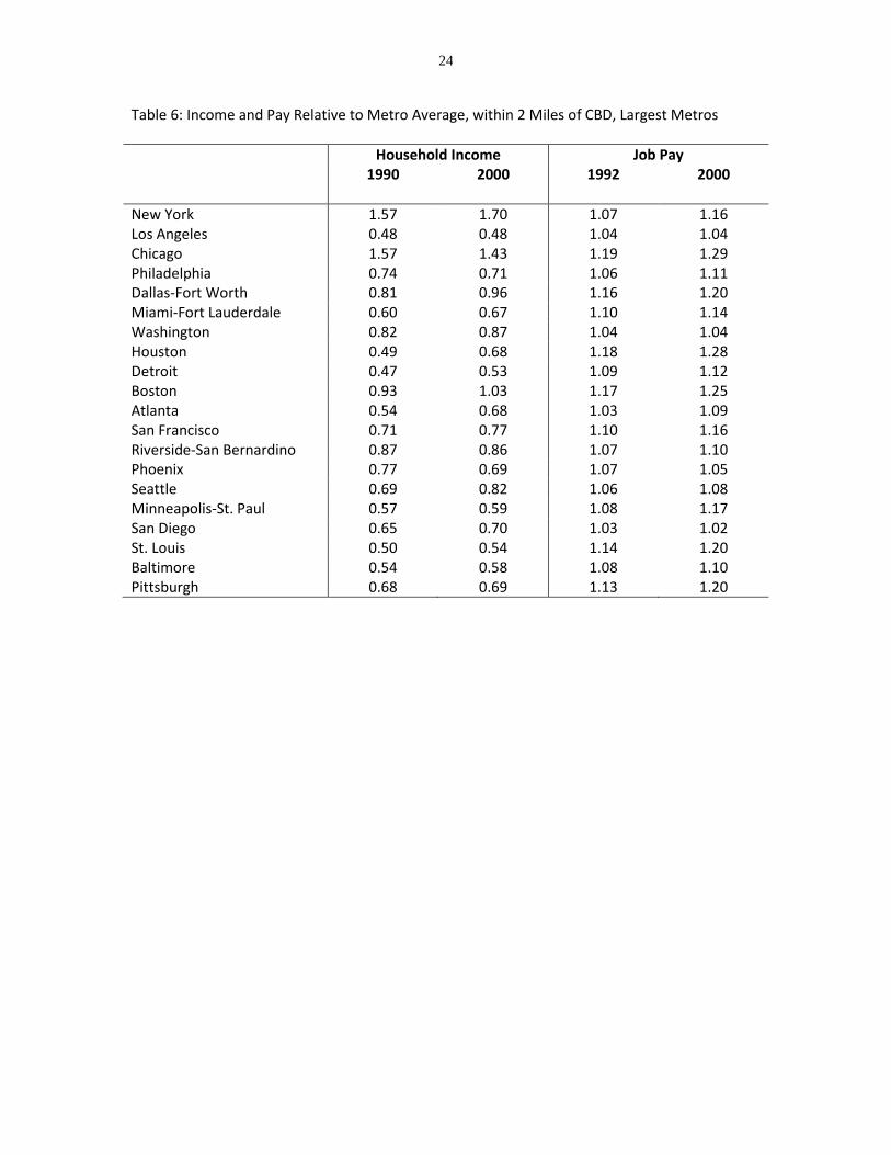
Higher-pay industries locate closer to downtowns in all of the largest
metropolitan areas, even though these areas vary considerably in the relative income of
downtown residents. Table 6 shows that the ratio of household income within 2 miles of
the CBD relative to the metropolitan average in 1990 was over 1.5 in New York and
Chicago and under 0.5 in Los Angeles, Houston, and Detroit. Yet the ratio of downtown
job pay relative to the metro average in 1992 ranged only from 1.03 (San Diego and
Atlanta) to 1.19 (Chicago).
EMPIRICAL METHODOLOGY AND RESULTS
The key empirical question is whether changes in neighborhood employment
composition – measured by average job pay – affects residential composition –
measured by average household income. I first look at the tract level. Then, to assess
whether the tract-level relationship between changes in job pay and changes in
14 Table 5 includes only non-farm, non-government industries with national employment over 100,000, but the analysis elsewhere in the paper includes all industries in calculating job pay.
13
household income helps explain gentrification, I look across metropolitan areas to see
what affects the change in relative downtown household income.
Neighborhood change: tract-level analysis
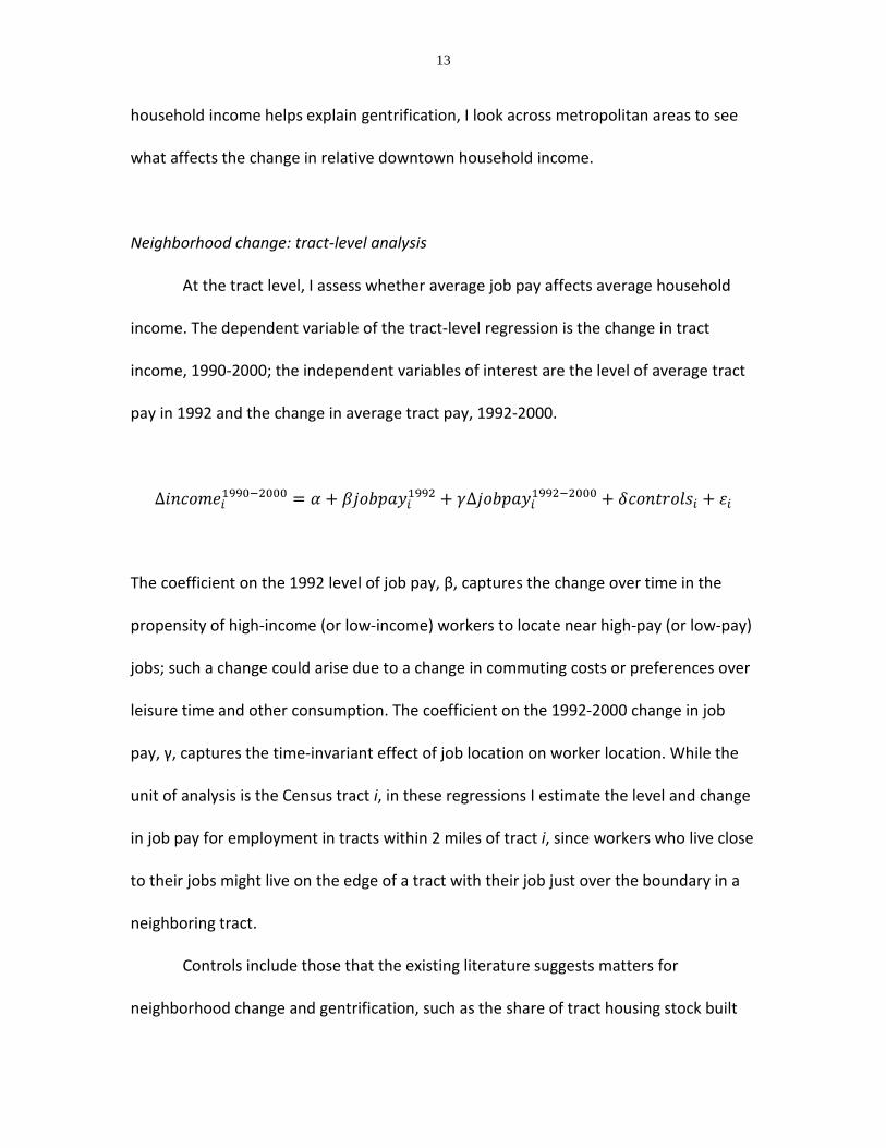
At the tract level, I assess whether average job pay affects average household
income. The dependent variable of the tract-level regression is the change in tract
income, 1990-2000; the independent variables of interest are the level of average tract
pay in 1992 and the change in average tract pay, 1992-2000.
The coefficient on the 1992 level of job pay, β, captures the change over time in the
propensity of high-income (or low-income) workers to locate near high-pay (or low-pay)
jobs; such a change could arise due to a change in commuting costs or preferences over
leisure time and other consumption. The coefficient on the 1992-2000 change in job
pay, γ, captures the time-invariant effect of job location on worker location. While the
unit of analysis is the Census tract i, in these regressions I estimate the level and change
in job pay for employment in tracts within 2 miles of tract i, since workers who live close
to their jobs might live on the edge of a tract with their job just over the boundary in a
neighboring tract.
Controls include those that the existing literature suggests matters for
neighborhood change and gentrification, such as the share of tract housing stock built

14
prior to 1940 (from housing filtering models), income in households of surrounding
tracts (tipping models), and tract household demographics, all in 1990 levels, as well as
average tract income in 1990 and 1980.15 Regressions are weighted by number of
households, include metropolitan-area fixed effects unless otherwise noted, and report
standard errors clustered by metropolitan area.
I estimate this model with OLS and, to handle potential endogeneity, I use two-
stage least squares. The potential endogeneity arises because people might follow jobs
and jobs might follow people; either one could account for a positive correlation
between the change in tract average income and the change in tract average job pay. An
appropriate instrument for the change in job pay would be (1) correlated with the
change in job pay and (2) have no independent effect on the change in average income.
In the 2SLS estimation, I instrument for the change in job pay with the predicted change
in job pay based on initial tract industry mix and national industry growth rates.16 In the
OLS estimation, the growth in average job pay in tract i equals (where j indexes
industries):
To instrument for this expression, I replace 2000 employment in the tract-industry cell
with predicted 2000 employment in the tract-industry cell:
15 Income in surrounding tracts is measured as the average income of the ten closest tracts, weighted by tract population and the inverse of the distance from the tract. 16 Dworak-Fisher (2004) instruments for regional employment growth in a similar way.
15
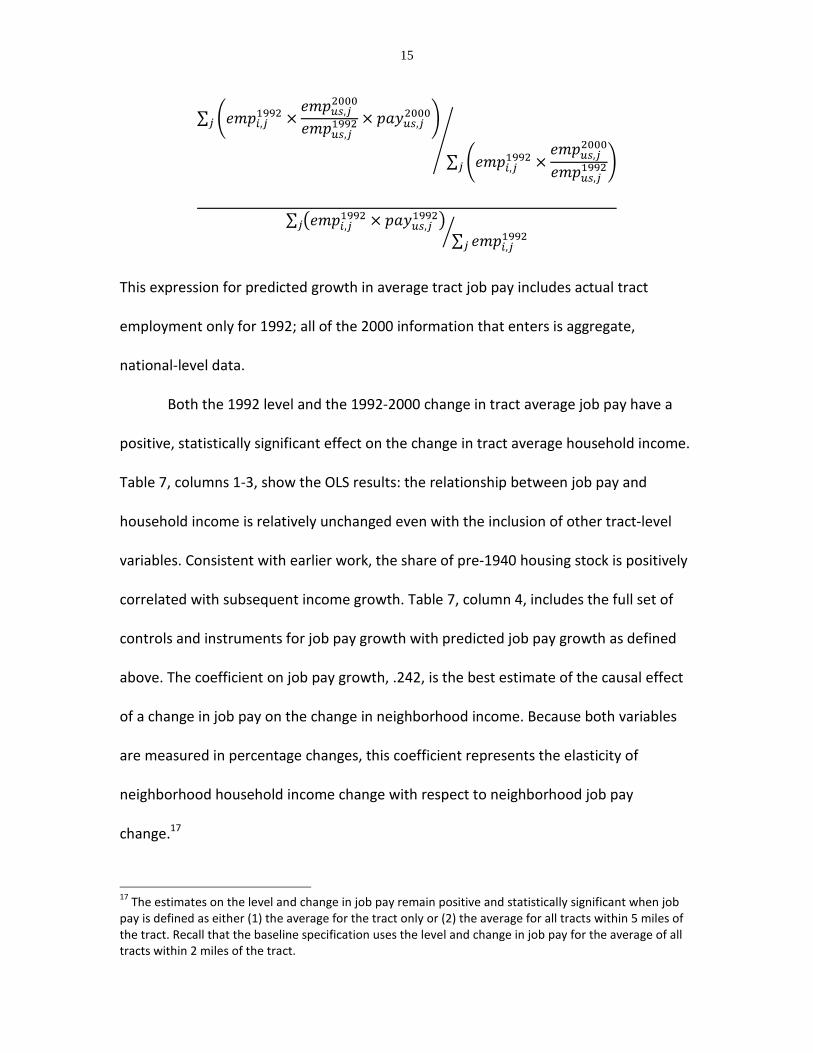
This expression for predicted growth in average tract job pay includes actual tract
employment only for 1992; all of the 2000 information that enters is aggregate,
national-level data.
Both the 1992 level and the 1992-2000 change in tract average job pay have a
positive, statistically significant effect on the change in tract average household income.
Table 7, columns 1-3, show the OLS results: the relationship between job pay and
household income is relatively unchanged even with the inclusion of other tract-level
variables. Consistent with earlier work, the share of pre-1940 housing stock is positively
correlated with subsequent income growth. Table 7, column 4, includes the full set of
controls and instruments for job pay growth with predicted job pay growth as defined
above. The coefficient on job pay growth, .242, is the best estimate of the causal effect
of a change in job pay on the change in neighborhood income. Because both variables
are measured in percentage changes, this coefficient represents the elasticity of
neighborhood household income change with respect to neighborhood job pay
change.17
17 The estimates on the level and change in job pay remain positive and statistically significant when job pay is defined as either (1) the average for the tract only or (2) the average for all tracts within 5 miles of the tract. Recall that the baseline specification uses the level and change in job pay for the average of all tracts within 2 miles of the tract.

16
The level and growth of job pay have a similarly strong, positive effect on income
growth without fixed effects. Table 7, column 5, shows that the results on job pay – and
on most other variables – are largely unchanged when omitting metropolitan-area fixed
effects. One notable exception is that the college-educated share now helps explain
neighborhood income growth – consistent with the established finding that education
and growth are correlated at the metropolitan-area level – even though the relationship
is much weaker at the tract level within metropolitan areas.
Different factors could affect neighborhood change in larger and smaller cities,
as well as in central and more suburban or exurban tracts. Table 8 repeats the 2SLS
regression, with metropolitan-area fixed effects, for two divisions of tracts. The first
column presents the model for each metropolitan area’s quartile of tracts (weighted by
households) closest to the CBD; the second column includes the second, third, and
fourth quartile of tracts from the CBD. The third column includes all tracts in
metropolitan areas larger than one million population; the fourth column includes all
tracts in metropolitan areas smaller than one million population. Comparing columns
one and two, both the level and growth of job pay have a much larger effect on
neighborhood income in central tracts than in tracts farther from the CBD. The
magnitude of the job pay level coefficient is only one-third the size in farther-out tracts
(column 2) as in central tracts (column 1), and the job pay change coefficient is not
statistically significant for the farther-out tracts. Comparing columns three and four,
both the level and growth of job pay are positive and statistically significant in

17
metropolitan areas larger than one million population; these coefficients are smaller
and statistically insignificant for tracts in smaller metropolitan areas.
Gentrification: metropolitan-level analysis
The second part of the empirical approach is a metropolitan-level analysis that
parallels the tract-level analysis. The metropolitan-level analysis helps us understand the
causes of gentrification. Gentrification is one possible manifestation of neighborhood
change, which occurs when tracts closer to the CBD exhibit faster income growth than
tracts farther from the CBD. Income growth in individual tracts near the CBD does not,
by itself, imply metropolitan-level gentrification, unless it results in a shift in the overall
relationship between average income and distance from the CBD. As Tables 1 and 2
show, gentrification has occurred only in larger metropolitan areas and only in the area
within 2 miles of the CBD. Table 6 shows that notable gentrification during the 1990’s
occurred in Dallas, Houston, Atlanta, and other places – where relative income within 2
miles of the CBD rose between 1990 and 2000.
In the metropolitan-level analysis, this change in relative “downtown” income is
the dependent variable. I use two different definitions of gentrification, corresponding
to how “downtown” is defined: relative income growth within 2 miles of the CBD, and
relative income growth within 5 miles of the CBD, to assess the sensitivity of the results.
The empirical specification is the same as in the previous section, but the unit of analysis
is the metropolitan area instead of the tract. The dependent and explanatory variables
are all expressed in terms of the downtown value – within 2 miles or within 5 miles of
the CBD -- relative to the metropolitan area value. Thus, the job pay growth variable

18
equals the ratio of job pay growth downtown to job pay growth in the metropolitan
area. Once again, I include both the level and growth of job pay, as well as pre-1940
housing stock and demographic variables.18 As before, I instrument for job pay growth
using national industry growth over 1992-2000 and national industry pay in 1992 and
2000, all applied to the 1992 industry mix.
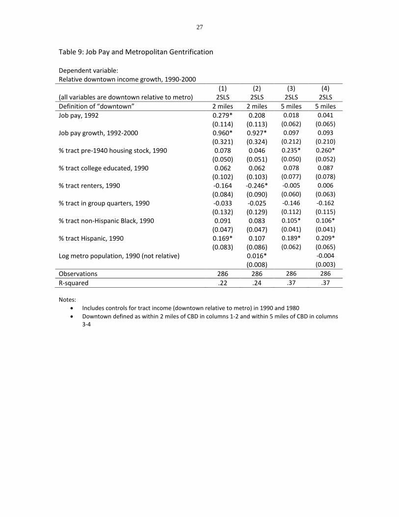
Table 9 shows that faster job pay growth in downtown areas does contribute to
gentrification within 2 miles of the CBD but not within 5 miles of the CBD. The
coefficient on job pay growth is positive and statistically significant in the 2SLS model,
including when log metropolitan population is added to the regression (column 2).
Because this coefficient and the dependent variable are percentage changes, the
coefficient represents an elasticity near one – a large effect. The coefficient on the level
of job pay is statistically significant only at the 10% level when log metropolitan
population is included but significant at the 5% level when population is excluded.
Defining gentrification as relative growth within 5 miles of the CBD, neither the level nor
growth of job pay has an effect (columns 3 and 4). An alternative explanation for
gentrification, older housing stock, does not explain gentrification within 2 miles of the
CBD but has a positive and statistically significant effect on metropolitan gentrification
using the 5-mile definition. The factors explaining gentrification, therefore, are sensitive
to how metropolitan gentrification is defined.
DISCUSSION AND CONCLUSION
18 I omit the neighboring tract income variable since a tract’s neighbors are in the same metropolitan area and therefore are included in the same observation.

19
Changes in average neighborhood job pay affect tract income growth, suggesting
that people follow jobs to some extent. The level of neighborhood job pay also affects
subsequent tract income growth, consistent with a changing preference for workers to
live closer to their jobs, which could arise from changes in the demand for housing or in
commuting costs. Because I do not observe micro-data on individual workers’ pay,
residential address, and job location, I cannot tell whether people locate near their own
jobs or whether higher-income households locate near jobs in higher-paying industries
for other reasons – such as proximity to jobs in order to minimize job search costs or
proximity to neighborhood amenities consumed by both higher-income households and
employees in higher-pay industries. Regardless, the findings show that higher-income
people follow jobs in higher-paying industries.
The relationship between job pay and household income is stronger in tracts
nearer the CBD and in tracts in large metros; in these tracts, commuting costs per mile
traveled are higher than tracts elsewhere. Downtowns have more expensive parking
and slower driving speeds, both of which raise the value to downtown employees to live
near work relative to employees whose jobs are elsewhere. Larger metros are more
congested (Schrank and Lomax, 2007), raising the value of large-metro residents to live
near work relative to small-metro residents. In places where commuting costs increase
less with respect to distance – outside central parts of cities and in smaller metropolitan
areas -- living near work is worth less.19 The weakening of the relationship between job
19 Many of the other explanations for neighborhood change – such as the share pre-1940 housing stock and average income of surrounding tracts – have roughly the same effect on tract income growth regardless of distance from the CBD and metropolitan area population; not surprisingly, these other explanations are independent of congestion or commuting costs.
20
pay and household income farther from the CBD is consistent with the mixed results for
metropolitan-area gentrification. Changes in relative downtown pay affect changes in
relative downtown income only when “downtown” includes tracts within 2 miles of the
CBD. Within 2 miles of the CBD, the relationship between job pay and tract income is
strong. The area within 5 miles of the CBD, however, includes tracts where the
relationship between job pay and tract income is weaker. The effect of job pay levels
and growth on relative downtown income is very sensitive to whether “downtown”
includes tracts within 2 miles or within 5 miles of the CBD.
An important implication of this paper is that national or global structural
changes – like the rise of finance or the decline of manufacturing – can trigger
neighborhood change. Neighborhood fortunes are tied to broader economic shifts.
Filtering models, in contrast, imply that gentrification is part of a natural process of
capital deterioration and re-investment; commuting-cost explanations imply that local
investments, like new transit nodes, can affect gentrification. There is, however, nothing
inevitable or locally-determined about neighborhood change induced by sectoral shifts.
For example, in the current recession, the shrinking finance sector – which is high-pay
and centrally located -- might reverse income growth in many downtown
neighborhoods and could retard or reverse gentrification in finance-heavy areas like
New York, Chicago, and Boston. The future of neighborhoods and of gentrification
depends, in part, on where industries locate and grow.
21
Table 1: Tract Average Household Income Relative to Metro Average, by Distance from CBD, 1980-2000 Distance from CBD 1980 1990 2000
Within 2 miles .80 .79 .80 2 to 5 miles .93 .91 .90 5 to 10 miles 1.03 1.01 .98 10 to 20 miles 1.08 1.09 1.08 20 or more miles 1.02 1.02 1.04 Table 2: Tract Average Household Income Relative to Metro Average, by Distance from CBD, 1980-2000, Metros with More Than One Million Population Only Distance from CBD 1980 1990 2000
Within 2 miles .76 .82 .89 2 to 5 miles .82 .80 .81 5 to 10 miles .99 .94 .91 10 to 20 miles 1.11 1.11 1.09 20 or more miles 1.04 1.05 1.06
22
Table 3: Tract Average Annual Job Pay Relative to Metro Average, by Distance from CBD, 1992 and 2000 Distance from CBD 1992 2000
Within 2 miles 1.07 1.10 2 to 5 miles 1.00 .99 5 to 10 miles .98 .98 10 to 20 miles .99 .99 20 or more miles .97 .96 Table 4: Tract Average Annual Job Pay Relative to Metro Average, by Distance from CBD, 1992 and 2000, Metros with More Than One Million Population Only Distance from CBD 1992 2000
Within 2 miles 1.09 1.14 2 to 5 miles 1.01 .99 5 to 10 miles .98 .98 10 to 20 miles .99 .99 20 or more miles .97 .96

23
Table 5: Industries with Highest and Lowest Share of Employment in Downtowns Industry Share within 2 miles
of CBD, 1992 Average pay, 1992
Highest share in downtowns Funds and trusts 38.3% 37544 Rail transportation 37.4% 25987 Securities and commodities 37.0% 85726 Credit Intermediation 31.7% 30033 Management of companies and enterprises 31.2% 43709 Publishing industries 29.3% 33051 Oil and gas extraction 28.9% 53565 Utilities 28.0% 41282 Insurance 27.3% 34521 Museums and historical sites 26.7% 19982 Lowest share in downtowns Fabricated metal product manufacturing 7.6% 29143 Specialty trade contractors 7.3% 25986 Truck transportation 7.1% 26390 Food and beverage stores 7.1% 14582 Gasoline stations 7.1% 12079 Furniture manufacturing 7.0% 21640 Wood product manufacturing 6.8% 22563 Building material and garden equipment dealers 6.6% 19758 Plastics and rubber product manufacturing 6.4% 27485 Computers and electronic product manufacturing 5.1% 39607 NAICS 3-digit industries, ranked by share within 2 miles of CBD. Industries with fewer than 100,000 employees nationally, agricultural industries, and public-sector industries are excluded from this table but included in the analysis.
24
Table 6: Income and Pay Relative to Metro Average, within 2 Miles of CBD, Largest Metros Household Income Job Pay 1990 2000
1992 2000
New York 1.57 1.70 1.07 1.16 Los Angeles 0.48 0.48 1.04 1.04 Chicago 1.57 1.43 1.19 1.29 Philadelphia 0.74 0.71 1.06 1.11 Dallas-Fort Worth 0.81 0.96 1.16 1.20 Miami-Fort Lauderdale 0.60 0.67 1.10 1.14 Washington 0.82 0.87 1.04 1.04 Houston 0.49 0.68 1.18 1.28 Detroit 0.47 0.53 1.09 1.12 Boston 0.93 1.03 1.17 1.25 Atlanta 0.54 0.68 1.03 1.09 San Francisco 0.71 0.77 1.10 1.16 Riverside-San Bernardino 0.87 0.86 1.07 1.10 Phoenix 0.77 0.69 1.07 1.05 Seattle 0.69 0.82 1.06 1.08 Minneapolis-St. Paul 0.57 0.59 1.08 1.17 San Diego 0.65 0.70 1.03 1.02 St. Louis 0.50 0.54 1.14 1.20 Baltimore 0.54 0.58 1.08 1.10 Pittsburgh 0.68 0.69 1.13 1.20

25
Table 7: Job Pay and Neighborhood Change Dependent variable: tract income growth, 1990-2000
(1) (2) (3) (4) (5) OLS OLS OLS 2SLS 2SLS Job pay, 1992, 2-mile circle 0.382* 0.286* 0.339* 0.360* 0.397* (0.123) (0.119) (0.084) (0.087) (0.107) Job pay growth, 1992-2000, 2-mile circle 0.162* 0.158* 0.140* 0.242* 0.282* (0.032) (0.032) (0.025) (0.099) (0.104) % tract pre-1940 housing stock, 1990 0.106* 0.152* 0.152* 0.108* (0.016) (0.019) (0.019) (0.023) Neighboring tract income, 1990 0.287* 0.280* 0.200* (0.021) (0.025) (0.032) % tract college educated, 1990 0.040 0.036 0.122* (0.027) (0.025) (0.023) % tract renters, 1990 -0.111* -0.114* -0.134* (0.013) (0.013) (0.017) % tract in group quarters, 1990 0.047* 0.047* 0.030 (0.022) (0.022) (0.024) % tract non-Hispanic Black, 1990 0.034* 0.034* 0.028 (0.011) (0.010) (0.015) % tract Hispanic, 1990 0.074* 0.075* 0.015 (0.012) (0.013) (0.026) Metro area fixed effects? Yes Yes Yes Yes No Observations 49199 49199 49199 49199 49199 R-squared .03 .04 .08 .08 .08 Notes:
• Weighted by 1990 households • Standard errors clustered by metro area • Includes controls for tract income in 1990 and 1980 • Centered R-squared reported even when excluding fixed effects

26
Table 8: Job Pay, Neighborhood Change, and Tract Characteristics Dependent variable: tract income growth, 1990-2000
(1) (2) (3) (4) 2SLS 2SLS 2SLS 2SLS Nearest
quartile of tracts to CBD
Farthest three
quartiles of tracts
from CBD
Metros larger than 1 million
Metros smaller than 1 million
Job pay, 1992, 2-mile circle 0.545* 0.180* 0.411* 0.087 (0.151) (0.069) (0.084) (0.079) Job pay growth, 1992-2000, 2-mile circle 0.456* 0.054 0.244* 0.128 (0.154) (0.081) (0.121) (0.082) % tract pre-1940 housing stock, 1990 0.142* 0.146* 0.155* 0.121* (0.013) (0.022) (0.026) (0.015) Neighboring tract income, 1990 0.271* 0.309* 0.249* 0.346* (0.026) (0.029) (0.030) (0.024) % tract college educated, 1990 0.074 -0.003 0.063 -0.023 (0.042) (0.020) (0.034) (0.039) % tract renters, 1990 -0.038* -0.151* -0.096* -0.177* (0.016) (0.011) (0.015) (0.021) % tract in group quarters, 1990 -0.006 0.080* 0.089* 0.031 (0.028) (0.026) (0.033) (0.023) % tract non-Hispanic Black, 1990 0.076* -0.011 0.024* 0.077* (0.010) (0.012) (0.011) (0.013) % tract Hispanic, 1990 0.100* 0.020 0.068* 0.074* (0.024) (0.017) (0.015) (0.026) Observations 13434 35764 32865 16334
R-squared .10 .09 .08 .10 Notes:
• Weighted by 1990 households • Includes metro area fixed effects • Standard errors clustered by metro area • Includes controls for tract income in 1990 and 1980
27
Table 9: Job Pay and Metropolitan Gentrification Dependent variable: Relative downtown income growth, 1990-2000
(1) (2) (3) (4) (all variables are downtown relative to metro) 2SLS 2SLS 2SLS 2SLS Definition of “downtown” 2 miles 2 miles 5 miles 5 miles Job pay, 1992 0.279* 0.208 0.018 0.041 (0.114) (0.113) (0.062) (0.065) Job pay growth, 1992-2000 0.960* 0.927* 0.097 0.093 (0.321) (0.324) (0.212) (0.210) % tract pre-1940 housing stock, 1990 0.078 0.046 0.235* 0.260* (0.050) (0.051) (0.050) (0.052) % tract college educated, 1990 0.062 0.062 0.078 0.087 (0.102) (0.103) (0.077) (0.078) % tract renters, 1990 -0.164 -0.246* -0.005 0.006 (0.084) (0.090) (0.060) (0.063) % tract in group quarters, 1990 -0.033 -0.025 -0.146 -0.162 (0.132) (0.129) (0.112) (0.115) % tract non-Hispanic Black, 1990 0.091 0.083 0.105* 0.106* (0.047) (0.047) (0.041) (0.041) % tract Hispanic, 1990 0.169* 0.107 0.189* 0.209* (0.083) (0.086) (0.062) (0.065) Log metro population, 1990 (not relative) 0.016* -0.004 (0.008) (0.003) Observations 286 286 286 286
R-squared .22 .24 .37 .37 Notes:
• Includes controls for tract income (downtown relative to metro) in 1990 and 1980 • Downtown defined as within 2 miles of CBD in columns 1-2 and within 5 miles of CBD in columns
3-4
28
REFERENCES
Aaronson, Daniel. 2001. “Neighborhood Dynamics.” Journal of Urban Economics 39: 1-
31. Bailey, Martin. 1959. “Note on the Economics of Residential Zoning and Urban
Renewal.” Land Economics 35: 288-292. Black, Dan, et al. 2002. “Why Do Gay Men Live in San Francisco?” Journal of Urban
Economics 51: 54-76. Boarnet, Marlon. 1994. “The Monocentric Model and Employment Location.” Journal of
Urban Economics 36: 79-97. Bond, Eric W., and N. Edward Coulson. 1989. “Externalities, Filtering, and Neighborhood
Change.” Journal of Urban Economics 26: 231-249. Bourne, Larry S. 1981. The Geography of Housing. New York: John Wiley and Sons. Brueckner, Jan. 1987. “The Structure of Urban Equilibria: A Unified Treatment of the
Muth-Mills Model.” Handbook of Regional and Urban Economics, Vol. II. Ed. E.S. Mills. Elsevier.
Brueckner, Jan, and Stuart Rosenthal. 2009. “Gentrification and Neighborhood Cycles:
Will America’s Future Downtowns Be Rich?” Review of Economics and Statistics, forthcoming.
Cooke, Timothy. 1978. “Causality Reconsidered: A Note.” Journal of Urban Economics 5:
538-542. Dworak-Fisher, Keenan. 2004. “Intra-Metropolitan Shifts in Labor Demand and the
Adjustment of Local Markets.” Journal of Urban Economics 55: 514-533. Fu, Shihe. 2006. “Sexual Orientation and Neighborhood Quality: Do Same-Sex Couples
Make Better Communities?” Unpublished working paper. Galster, George C. 1990. “Neighborhood Racial Change, Segregationist Sentiments, and
Affirmative Marketing Policies.” Journal of Urban Economics 27: 334-361. Galster, George, Roberto Quercia, Alvaro Cortes, and Ron Malega. 2003. “The Fortunes
of Poor Neighborhoods.” Urban Affairs Quarterly 39: 205-227.
29
Glaeser, Ed, Matthew Kahn, and Jordan Rappaport. 2008. “Why Do the Poor Live in Cities? The Role of Public Transportation.” Journal of Urban Economics 63: 1-24.
Glaeser, Ed, Jed Kolko, and Albert Saiz. 2001. “Consumer City.” Journal of Economic
Geography 1: 27-50. Hammel, Daniel, and Elvin Wyly. 1996. “A Model for Identifying Gentrified Areas with
Census Data.” Urban Geography 17(3): 248-268. Helms, Andrew. 2003. “Understanding Gentrification: An Empirical Analysis of the
Determinants of Urban Housing Renovation.” Journal of Urban Economics 54: 474-498.
Ihlanfeldt, Keith, and David Sjoquist. 1998. “The Spatial Mismatch Hypothesis: A Review
of Recent Studies and Their Implications for Welfare Reform.” Housing Policy Debate 9(4): 849-892.
Kahn, Matthew. 2007. “Gentrification Trends in New Transit-Oriented Communities:
Evidence from 14 Cities That Expanded and Built Rail Transit Systems.” Real Estate Economics 35: 155-182.
Kern, Clifford. 1984. “Upper Income Residential Revival in the City: Some Lessons from
the 1960s and 1970s for the 1980s.” Research in Urban Economics, Vol. 4. JAI Press. 79-96.
Knopp, Lawrence. 1997. “Gentrification and Gay Neighborhood Formation in New
Orleans: A Case Study.” Homo Economics. Eds. Amy Gluckman and Betsy Reed. New York: Routledge, 45-64.
Kolko, Jed, and David Neumark. 2007. Business Location Decisions and Employment
Dynamics in California. San Francisco: Public Policy Institute of California. Lin, Jeffrey. 2002. “Gentrification and Transit in Northwest Chicago.” Journal of the
Transportation Research Forum 56: 175-191. Martin, Richard. 2001. “The Adjustment of Black Residents to Metropolitan Employment
Shifts: How Persistent is Spatial Mismatch?” Journal of Urban Economics 50: 52-76.
Muth, Richard. 1969. Cities and Housing. Chicago: University of Chicago Press. Muth, Richard. 1973. “A Vintage Model of the Housing Stock.” Papers of the Regional
Science Association 30: 141-156.
30
Myers, Dowell. 1990. “Filtering in Time: Rethinking the Longitudinal Behavior of Neighborhood Housing Markets.” Housing Demography: Linking Demographic Structure and Housing Markets. Ed. Myers. Madison, Wisconsin: University of Wisconsin Press. 274-296.
Rosenthal, Stuart. 2008. “Old Homes, Externalities, and Poor Neighborhoods: A Model
of Urban Decline and Renewal.” Journal of Urban Economics 63: 816-840. Schelling, Thomas. 1978. Micromotives and Macrobehavior. New York: W. W. Norton. Schrank, David, and Tim Lomax. 2007. “The 2007 Urban Mobility Report.” Texas
Transportation Institute. Steinnes, Donald. 1977. “Causality and Intraurban Location.” Journal of Urban
Economics 4: 69-79. Steinnes, Donald. 1982. “Do ‘People Follow Jobs’ or Do ‘Jobs Follow People’? A Causality
Issue in Urban Economics.” Urban Studies 19: 187-192. Weinberg, Bruce. 2004. “Testing the Spatial Mismatch Hypothesis Using Inter-City
Variations in Industrial Composition.” Regional Science and Urban Economics 34: 505-532.
Wheaton, William. 1977. “Income and Urban Residence: An Analysis of Consumer
Demand for Location.” American Economic Review 67: 620-631.
Top Related