


Languages
Pages
Legal


THE TI-NSPIRE PROGRAMS
JAMES KEESLING
The purpose of this document is to list and document the programs that will be used inthis class. For each program there is a screen shot containing an example and a listing ofthe TN-Nspire CX CAS program. The student is responsible to enter each program andbe familiar with its use.
1. Solving f(x) = 0
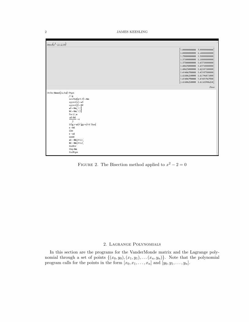
In this section are the Newton-Raphson method and the Bisection method.
Figure 1. The Newton-Raphson method applied to x2 − 2 = 0
1
2 JAMES KEESLING
Figure 2. The Bisection method applied to x2 − 2 = 0
2. Lagrange Polynomials
In this section are the programs for the VanderMonde matrix and the Lagrange poly-nomial through a set of points {(x0, y0), (x1, y1), . . . (xn, yn)}. Note that the polynomialprogram calls for the points in the form [x0, x1, . . . , xn] and [y0, y1, . . . , yn].

THE TI-NSPIRE PROGRAMS 3
Figure 3. Program for the VanderMonde matrix for the points {1, 2, 3}
Figure 4. The Lagrange polynomial through the points {(0, 1), (1, 0), (3, 2)}
4 JAMES KEESLING
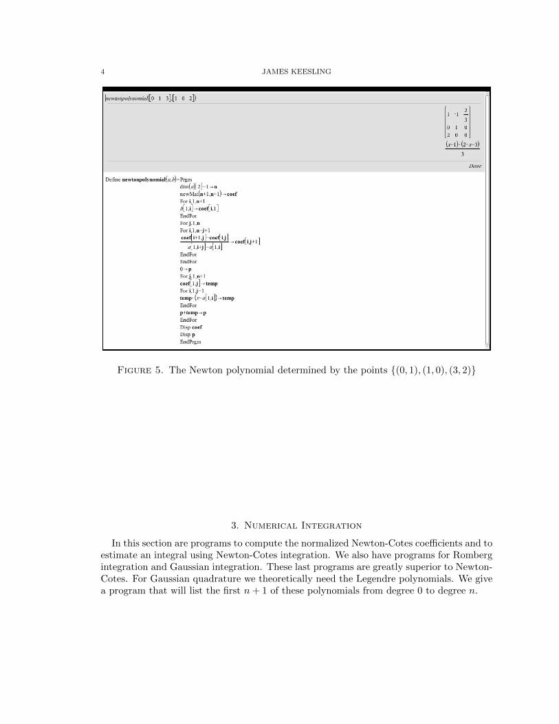
Figure 5. The Newton polynomial determined by the points {(0, 1), (1, 0), (3, 2)}
3. Numerical Integration
In this section are programs to compute the normalized Newton-Cotes coefficients and toestimate an integral using Newton-Cotes integration. We also have programs for Rombergintegration and Gaussian integration. These last programs are greatly superior to Newton-Cotes. For Gaussian quadrature we theoretically need the Legendre polynomials. We givea program that will list the first n + 1 of these polynomials from degree 0 to degree n.
THE TI-NSPIRE PROGRAMS 5
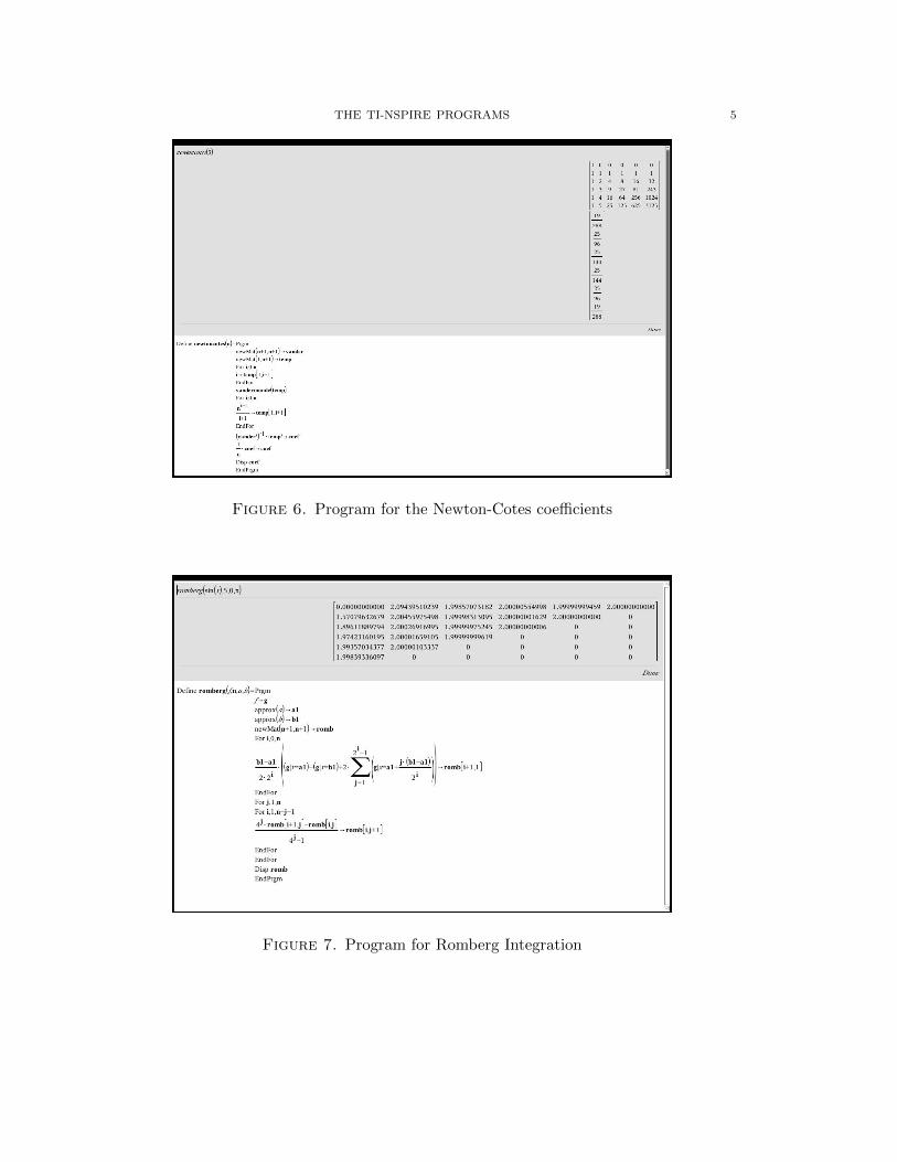
Figure 6. Program for the Newton-Cotes coefficients
Figure 7. Program for Romberg Integration

6 JAMES KEESLING
Figure 8. Program for Gaussian quadrature
Figure 9. Program for the Legendre polynomials up to degree n

THE TI-NSPIRE PROGRAMS 7
Figure 10. Program for n points and n coefficients for Gaussian quadrature
4. Numerical Differentiation
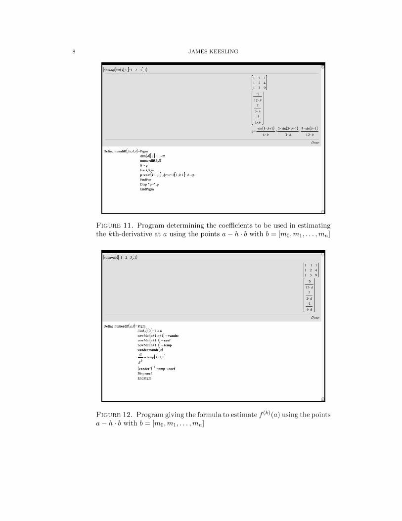
In this section we give the programs needed for numerical differentiation of a functionf(x). There are two of these programs. The first program determines the coefficients to
be used in estimating f (k)(a) using the n+ 1 points {a−m0 ·h, a−m1 ·h, · · · , a−mn ·h}.In the programs b = [m0,m1, . . . ,mn]
8 JAMES KEESLING
Figure 11. Program determining the coefficients to be used in estimatingthe kth-derivative at a using the points a− h · b with b = [m0,m1, . . . ,mn]
Figure 12. Program giving the formula to estimate f (k)(a) using the pointsa− h · b with b = [m0,m1, . . . ,mn]

THE TI-NSPIRE PROGRAMS 9
5. Differential Equations
In this section we give some programs useful for solving ordinary differential equations.We give a theoretical solution based on Picard iteration and numerical methods based somemethod of integration. We also give a program for the Taylor method.
Figure 13. Program giving the Picard iteration method

10 JAMES KEESLING
Figure 14. Example using the Taylor method
Figure 15. Program for the Taylor method
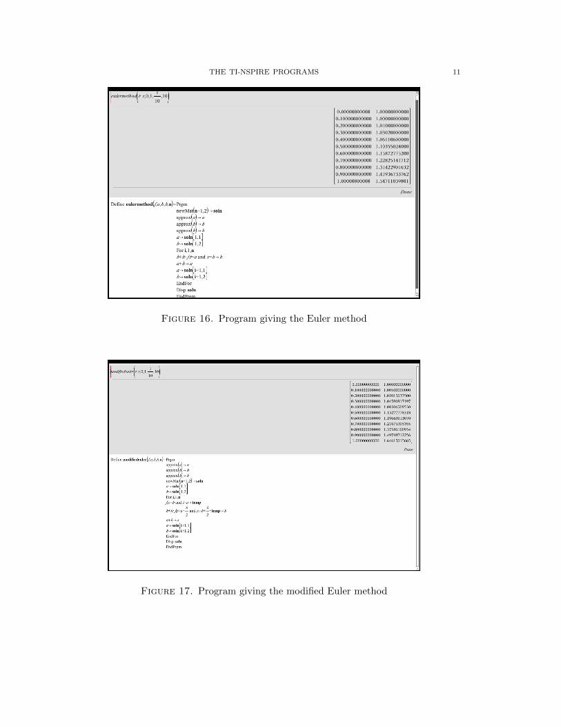
THE TI-NSPIRE PROGRAMS 11
Figure 16. Program giving the Euler method
Figure 17. Program giving the modified Euler method

12 JAMES KEESLING
Figure 18. Program giving the Heun method
Figure 19. Program giving the Runge-Kutta method

THE TI-NSPIRE PROGRAMS 13
6. Stochastic Simulation
In this section we do not show copies of the programs. They can now be downloaded.So, there is no need for them to be given to be copied into your calculator. However, wedo give examples of how the data is to be entered when the programs are run and whatthe typical output will look like and how it should be interpreted.
Figure 20. Program giving an example of the Bowling program. Theoutput is a sequence of scores for a bowler whose probability of a strike,spare, and open frame are the numbers entered in that order.

14 JAMES KEESLING
Figure 21. Program giving an example of the Queue simulation program.The output gives the time spent in each state given the arrival rate, theservice rate, and the number of servers.

THE TI-NSPIRE PROGRAMS 15
Figure 22. This program estimates the integral∫ ba dx by the Monte Carlo
method using n random points in the interval [a, b]. It gives k estimates ofthe integral.
Top Related