


Languages
Pages
Legal


INSTITUTE OF AERONAUTICAL ENGINEERING
IV B. Tech I semester (JNTUH-R15)Experimental Aerodynamics
Elective II
(Autonomous)
Dundigal, Hyderabad -500 043
AERONAUTICAL ENGINEERING
Prepared by
Shiva Prasad U,Assistant Professor, AE
iare 1

iare 2

Wind Tunnels
• Objective
• Accurately simulate the fluid flow aboutatmospheric vehicles
• Measure -Forces, moments, pressure, shearstress, heat transfer, flowfield (velocity, pressure,vorticity, temperature)
iare 3

Low Speed Vehicles - M<.3
U
Gallilean Transformation
Flight in atmosphereScale =L
Wind Tunnel - Model Scale =
IssuesFlow Quality - Uniformity and
Turbulence LevelWind Tunnel Wall InterferenceReynolds Number Simulation
U
ULU
Re
Stationary Walls
iare 4

Transonic Regime .7<M<1.2
• Must Match Reynolds Number and Mach Number
c
UM
LU
Re
Must change fluid density and viscosity to match Re and M
Cryogenic Wind Tunnels are designed for this reason
iare 5

History
Whirling Arm
iare 6
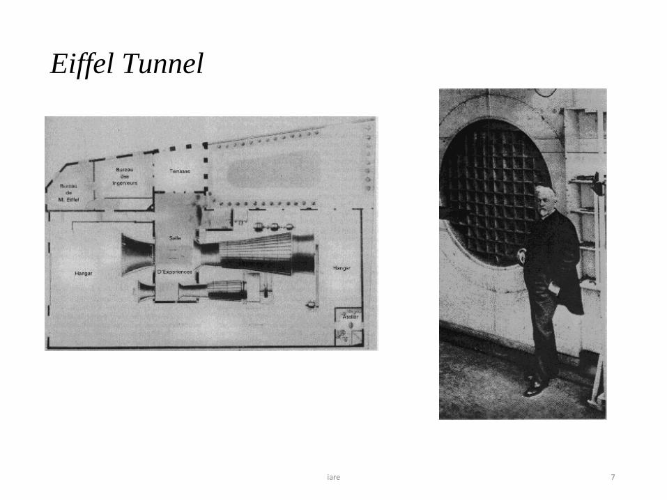
Eiffel Tunnel
iare 7

Wright Brothers
iare 8

iare 9

Wind Tunnel Layout
• Closed Return
• Open Return
• Double Return
• Annular Return
iare 10
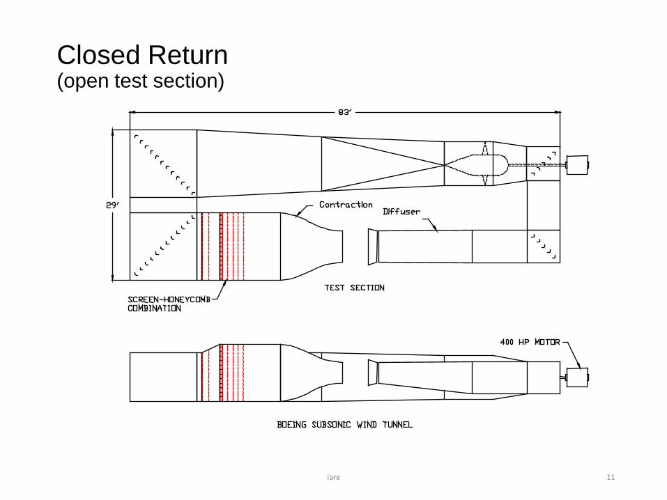
Closed Return(open test section)
iare 11

Open ReturnClosed Test Section
1 5 H p . D u a l
C e n trifu g a l B lo w e r
E xhaus t
E xhaus t
L o uvers
fo r S p eed
A d jus tm en t
T e s t S e c tio n
1 8 in c h D ia m e te r
2 5 to 1 C o n tra c tio n
S c re e n s H ig h C o n tr a c tio n W in d T u n n e l
T o p V ie w
D iffu s e r
iare 12

Double Return
U N I V E R S I T Y OF W A S H I N G T O NA E R O N A U T I C A L L A B O R A T O R Y
Kirsten Wind Tunnel
iare 13

Annular WindTunnel
iare 14

Types of Wind Tunnels
• Subsonic
• Transonic
• Supersonic
• Hypersonic
• Cryogenic
• Specialty• Automobiles• Environmental- Icing, Buildings, etc.
iare 15

Subsonic Wind Tunnels
iare 16

40’ x 80’ and 80’ x 120’NASA Ames
iare 17
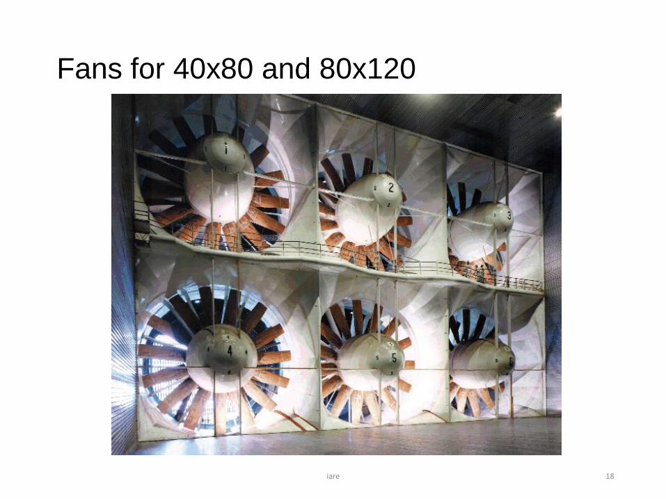
Fans for 40x80 and 80x120
iare 18

40’x80’ 80’x120;
iare 19

12 foot Pressure Tunnel
iare 20

iare 21

12-Foot Pressure Wind Tunnel: Specifications
Primary Use:The facility is used primarily for high Reynolds number testing, including the development of high-lift systems for commercial transports and military aircraft, high angle-of-attack testing of maneuvering aircraft, and high Reynolds number research.
Capability:Mach Number: 0-0.52 Reynolds Number per foot: 0.1 - 12X106 Stagnation Pressure, PSIA: 2.0 - 90 Temperature Range: 540 ° - 610 ° R
iare 22

TransonicWind Tunnels
iare 23

Transonic Wind Tunnels
Wall interference is a severe problem for transonicwind tunnels.Flow can “choke”
Shock wave across the tunnel test section
Two SolutionsPorous WallsMovable Adaptive Walls
iare 24

iare 25

iare 26

iare 27

Principle Operation Detonation Driven Shock TunnelSet- up and wave plan:
Initial conditions:• low pressure section: test gas air, about 25 kPa for tailored cond.• deton. section: oxyhydrogen- helium/ argon mixtures, max. 7 MPa• damping section: expansion volume; low initial pressures
iare 28

iare 29

iare 30

CryogenicWind Tunnels
iare 31

iare 32

NATIONAL TRANSONIC FACILITY
iare 33
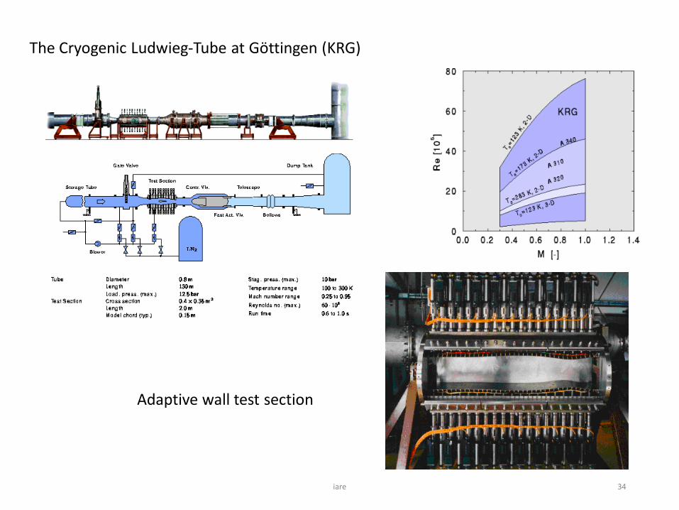
The Cryogenic Ludwieg-Tube at Göttingen (KRG)
Adaptive wall test section
iare 34

AutomobileWind Tunnels
iare 35

iare 36

Energy Ratio
P
AUqAURE
t
Losses
2/1
LossesCircuit
EnergyJet .).(
0000
3
00
Subscript 0 refers to the test sectionP is the motor power
is the fan efficiency
Wind Tunnel Power Requirements
iare 37

Wind Tunnel Circuit Elements
iare 38

Losses
q
ppK
tt 21
Local Pressure Loss Coefficient
00
21
0
q
qK
q
ppK
tt
Pressure Loss Referred to Test Section
0
3
0002/1 AUKE Section Energy Loss
00
3
000
0
3
001
2/1K
2/1
LossesCircuit
EnergyJet .).(
KAU
AURE
t
iare 39

Closed Return Tunnel
iare 40

Example - Closed Return Tunnel
S e c tio n K o % T o ta l L o s s
1 T e s t S e c tio n .0 0 9 3 5 .1
2 D if fu se r .0 3 9 1 2 1 .3
3 C o rn e r # 1 .0 4 6 0 2 5 .0
4 S tra ig h t S e c tio n .0 0 2 6 1 .4
5 C o rn e r # 2 .0 4 6 0 2 5 .0
6 S tra ig h t S e c tio n .0 0 2 0 1 .1
7 D if fu se r .0 1 6 0 8 .9
8 C o rn e r # 3 .0 0 8 7 4 .7
9 C o rn e r # 4 .0 0 8 7 4 .7
1 0 S tra ig h t S e c tio n .0 0 0 2 .1
1 1 C o n tra c tio n .0 0 4 8 2 .7
T o ta l .1 8 3 4 1 0 0 .0
45.51834.
11.).(
0
KRE
t
iare 41

Example - Open Return Tunnel
S e c t io n K o % T o t a l L o ss
1 In le t In c lu d in g S c re e n s .0 2 1 1 4 .0
2 C o n tra c tio n a n d T e s t S e c tio n .0 1 3 8 .6
3 D if fu se r .0 8 0 5 3 .4
4 D isc h a rg e a t O u tle t .0 3 6 2 4 .0
T o ta l .1 5 0 1 0 0 .0
67.6150.
11.).(
0
KRE
t
iare 42

Turbulence Management System
Stilling Section - Low speed and uniform flow
Screens - Reduce Turbulence [Reduces Eddy size for Faster Decay]- Used to obtain a uniform test section profile- Provide a flow resistance for more stable fan operation
Honeycomb - Reduces Large Swirl Component of Incoming Flow
iare 43

Test Section
Test Section - Design criteria of Test Section Size and Speed Determine Rest of Tunnel Design
Test Section Reynolds NumberLarger JET - Lower Speed - Less Power - More Expensive
Section Shape - Round-Elliptical, Square, Rectangular-Octagonal with flats for windows-mounting platformsRectangular with filled cornersNot usable but requies power
For Aerodynamics Testing 7x10 Height/Width Ratio
Test Section Length - L = (1 to 2)w
iare 44

Corners
Abrupt Corner without Vanes 0.1
iare 45

Low Speed Wind Tunnels-Detailed Design
Unit 2
iare 46

Wind Tunnel Design
• Open-circuit or Straight through type.• Wright Brother’s tunnel
• simple & very efficient
• small open-circuit tunnels are usually inside a building• large tunnels must be open to outside are susceptible to
dust ect.• Open-circuit tunnels are very noisy & surrounded by high
wind current
iare 47

Wind Tunnel Design
• Closed-Circuit or Return Type• Air is accelerated by the fan and flows through the tunnel
• Turning vanes are installed to guide flow around the corner
• The tunnel widens into a large settling chamber to decelerate the air; preventing a large build up of large boundary layer along the wall
iare 48
Wind Tunnel Design
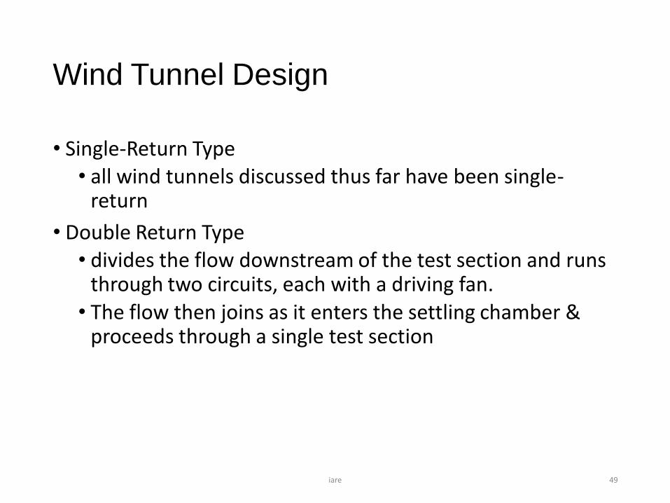
• Single-Return Type• all wind tunnels discussed thus far have been single-
return
• Double Return Type • divides the flow downstream of the test section and runs
through two circuits, each with a driving fan.• The flow then joins as it enters the settling chamber &
proceeds through a single test section
iare 49

Wind Tunnel Design
• Annular• An extension of the double-return concept
• A return passage is located around the entire circumference of the wind tunnel outside the test section
• This design was employed in the NACA variable density tunnel
iare 50

Wind Tunnel Design
• Spin Tunnel• Special type of annular tunnel employed at Langley
Research Center for spin research.• Is mounted vertically with the fan drawing air upward
• Models are introduced into free-flight conditions then vertical flow adjusted
iare 51

Types of Wind Tunnel Tests
• Original testing in wind tunnels was to a provide a means to determine lift & drag on airfoil shapes.
• Force Test• Force measurement requires a force to be exerted (lift &
drag forces so termed force test)• The balance can measure only two forces: lift & drag
iare 52

Six-Component Balance
• A more complete balance that can measure all six measures& moments about all three axes of the airplane
• Six component wind tunnel balance• this balance measures forces by use of strain gauges
iare 53
Types of Wind Tunnel Tests
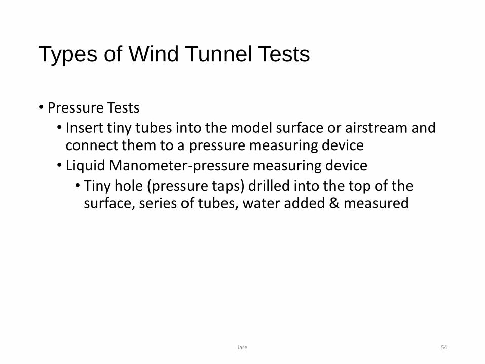
• Pressure Tests• Insert tiny tubes into the model surface or airstream and
connect them to a pressure measuring device• Liquid Manometer-pressure measuring device
• Tiny hole (pressure taps) drilled into the top of the surface, series of tubes, water added & measured
iare 54

Types of Wind Tunnel Tests
• Lowered pressure over the wing surface reduced the pressure in the manometer tubes and draws the water level up to a high level
• The lower the pressure, the higher the water level goes
• Measuring the difference in water level will show the relative pressure difference
iare 55

Types of Wind Tunnel Tests
• Flow Patterns• Allow the streamlines of air flow to look at the body’s
aerodynamic properties• Tufting allows for the flow pattern visualization
• Tufting –the attachment of small tufts of yarn to the surface
• The tufts will show if flow is attached or separated to form a wake.
iare 56

Types of Wind Tunnel Tests
• Flow pattern• visualized by the use of smoke at the Embry-Riddle
smoke tunnel• Smoke is generated by burning oil; then injected into into
the airstream
• Oil flow techniques can also be used to study flow patterns
iare 57

High Speed Wind Tunnels
• Supersonic tunnels-1st developed in Germany, Busemannwho also developed the swept-wing concept
• Early supersonic tunnels were the blow down type at Mach 1
• One of the most difficult conditions to create the flow atexactly Mach 1
iare 58

Wind Tunnel Testing Problems
• Wall Effect• Walls are artificial boundaries that airplanes do not have
• Upwash/downwash from walls, floors, ceiling
• Scale Effect• Small models have small forces making measurements
inaccurate• Differences in Reynolds number between model and the
full-scale model
iare 59

Flight Testing
• Shakedown Tests• Basic flight qualities are determined
• Airplane’s Performance• An exact determination of top speed, cruise speed, range,
rate of climb, takeoff & landing distance
• Stability & Controllability• Exact degree of stability, handling qualities
iare 60

Flight Testing
• Performance• Special instruments take measurements in test flights
• Pressure Measurements• Attaching pressure measuring devices to taps on the
aircraft surface
• Flow visualization• Tufts similar to wind tunnel testing• Reveal poor aerodynamic characteristics
iare 61

Unit 3High Speed Tunnels and
Low speed Balances
iare 62

• DH bearing pedestals are designed for the following applications:Low speed balancing
• Checking of rotor balance at high speeds (operational speed)
• Dynamic straightening of flexible rotors
• Testing of material strength by operating rotors at over speed
• Rotor investigation in operational bearings.
• All these tasks can be performed in a single rotor set up. The most important features of these high-speed balancing systems are shown on the next page.
iare 63

iare 64

• Rigid bearing supports – Additional stiffness
Rigid bearing supports provide for greater stability, particularly at high speeds. A supplementary, remote controlled change-over facility enables the stiffness of the bearing pedestals to be varied, thus enabling rotor resonance frequencies to be passed through safely, and minimizing the risk of damaging the rotor orthe balancing facility.
Balancing and overspeed testing under vacuumDue to the high windage effect of bladed rotors at high speeds and the associated power and temperatureproblems, balancing and overspeed testing takes place under vacuum conditions with a residual pressure of approx. 0.5 - 2 mbar.
iare 65
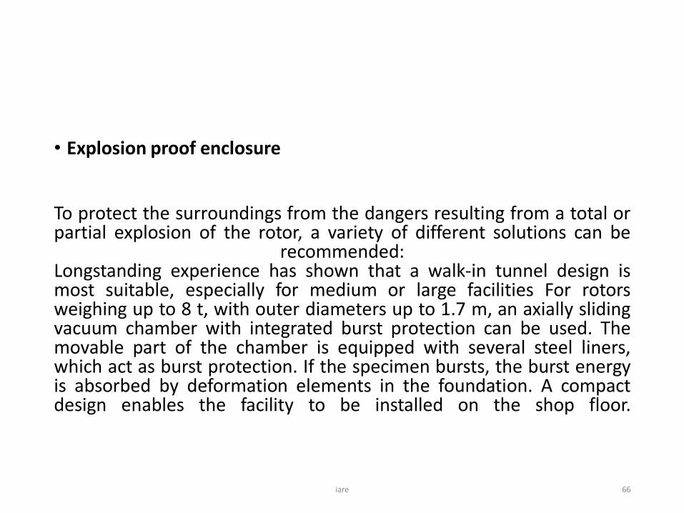
• Explosion proof enclosure
To protect the surroundings from the dangers resulting from a total orpartial explosion of the rotor, a variety of different solutions can be
recommended:Longstanding experience has shown that a walk-in tunnel design ismost suitable, especially for medium or large facilities For rotorsweighing up to 8 t, with outer diameters up to 1.7 m, an axially slidingvacuum chamber with integrated burst protection can be used. Themovable part of the chamber is equipped with several steel liners,which act as burst protection. If the specimen bursts, the burst energyis absorbed by deformation elements in the foundation. A compactdesign enables the facility to be installed on the shop floor.
iare 66

• Drive system
For high-speed balancing, overspeed testing and dynamicstraightening of flexible rotors, either a three-phase servomotor with frequency converter or an infinitely variable DCmotor with thyristor control can be used .Depending on the required speed range, a suitabletransmission gear has to be installed. A so-called intermediateshaft constitutes the connection between the gear and theover-speed testing chamber. Rotors are coupled to thisintermediate shaft by means of precision drive shafts.
iare 67

Automatic Balance Calibration System
• Complete calibration (including installation, preparation of loadschedule, load phase, full data reduction & balance removal)with 1000 loading points completed in about 3.5 hours.
• >0.1% accuracy preserved in any force combinations.
• Four safety loops ensure balance and machine integritythroughout the calibration.
• Calibration loads are applied exactly as in the wind tunnel formaximum calibration accuracy and reliability.
• Back-calculated errors can be displayed graphically in real timefor quick evaluation.
• Inherent reliability and long term accuracy.
• Calibration of single piece and two shell balances up to 2.5"diameter.
iare 68

Balances
• The balances are defined using aircraft design software (UGNX) and finite element software. The design is optimized according to customer-specified parameters (dimensions, loading and interfaces) and with respect to measurement requirements for sensitivity and stiffness.
• Balance Types:
• 6 component sting balance
• 1-5 component hinge moments balance
• 4-6 component fin balance
• Wing tip balance
• Half-model balance
iare 69

Balances
iare 70

General arrangement of A.R. g jet-flap model
• To illustrate various aspects of the test arrangement devised, it isconvenient to discuss the specific model details, the air-bearing rigassembly, and the recording system, in turn.
iare 71

Manual Procedure
• The normal running procedure was as follows.
• (a) The blowing pressure corresponding to the desired value of C, was set.
• (b) The wind-tunnel speed was set at the prescribed value, and the spring attachment bolts were adjusted to remove any yaw on the model-t due to asymmetric thrust or aerodynamic moment.
• (c) With positive damping, the model was manually forced by pulling cyclically on one of the wire/spring junctions until the amplitude was greater than + 6”, when the model was carefully released and the recorder started.1 The run was continued until the oscillations had damped out completely or had reached a small, steady, residual amplitude.
iare 72

Mechanical Design system balance
• Naturally, the problem of separating out the aerodynamiccomponents of the yawing moment is eased if the inertia componentcan be cancelled, or very much reduced, and a simple angularaccelerometer has been incorporated for this purpose.
• Strain-gauges on the leaf-springs are connected to give an outputcancelling that obtained from the model yawing-moment balancedue to the model inertia.
• The weights are adjusted wind-off to give approximate cancellation,leaving a small tare value which is measured at intervals to allow fordrift due mainly to temperature.
iare 73
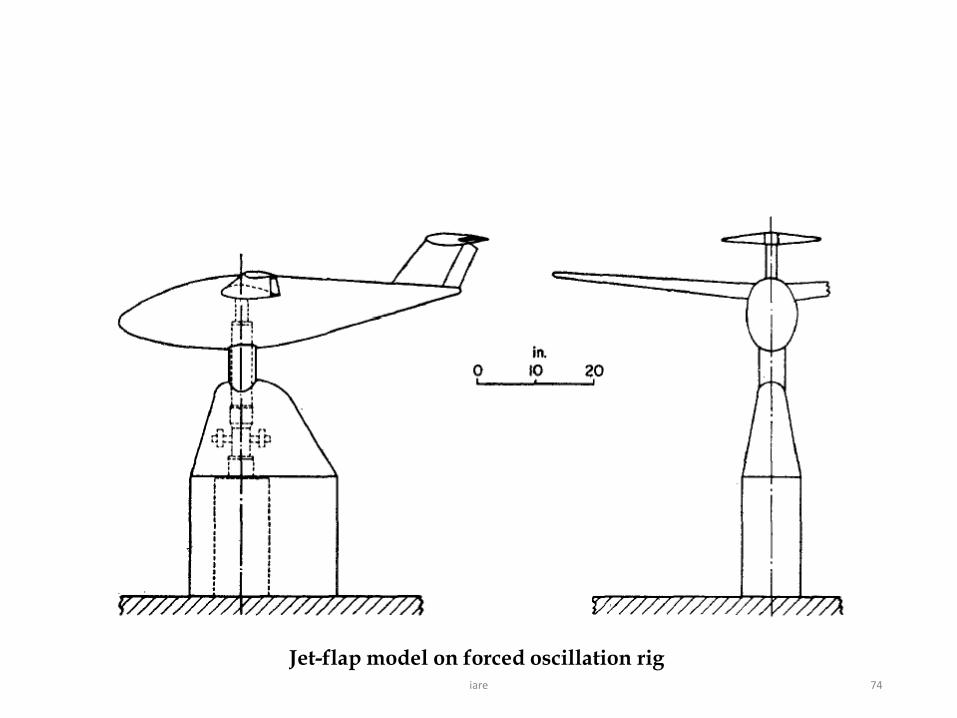
Jet-flap model on forced oscillation rigiare 74

Measurement of Pressure, Velocity and
TemperatureUnit 4
iare 75

Introduction
• Pressure measurement is important in many fluid mechanics relatedapplications.
• From appropriate pressure measurements velocity, aerodynamicforces and moments can be determined. Pressure is measured by theforce acting on unit area.
• Measuring devices usually indicate differential pressure i.e. inrelation with atmospheric pressure. This is called gauge pressure.
• The measured pressure may be positive or negative with reference tothe atmospheric pressure .A negative gauge pressure is referred to asvacuum.
iare 76

Pressure
iare 77
Pressure measuring devices
• Liquid column manometers
• Pressure gauges with elastic sensing elements
• Pressure transducers
• Manometers for low absolute pressures
• Manometers for very high absolute pressures
iare 78

Liquid column manometers
iare 79

Inclined manometer
Inclined manometer
iare 80

Mercury barometer
• Barometer is the device used to measure the atmosphericpressure.
• Mercury barometer consists essentially of a glass tubesealed at one end and mounted vertically in a bowl orcistern of mercury so that the open end of the tube issubmerged below the surface of mercury in the cistern.
iare 81

Principle of mercury barometer
iare 82

Micro manometer
iare 83

Mechanical manometers
• Bourdon tube
• Elastic diaphragms
• Corrugated diaphragms
• Capsules, Bellows
iare 84

Lag in manometric systems
Wind tunnel model with the manometric system
iare 85

Flow VisualizationUNIT- V
iare 86

Introduction
• The visualization of complex flows has played a uniquely importantrole in the improvement of our understanding of fluid dynamicphenomena.
• Flow visualization has been used to verify existing physical principlesand has led to the discovery of numerous flow phenomena.
• In addition to obtaining qualitative global pictures of the flow thepossibility of acquiring quantitative measurements withoutintroducing probes that invariably disturb the flow has provided thenecessary incentive for development of a large number ofvisualization techniques.
• The role of flow visualization in experimental fluid-mechanicalresearch has been appraised many times, and a number of reviews orcomprehensive descriptions, either of the whole field or particularapplications, are available.
iare 87
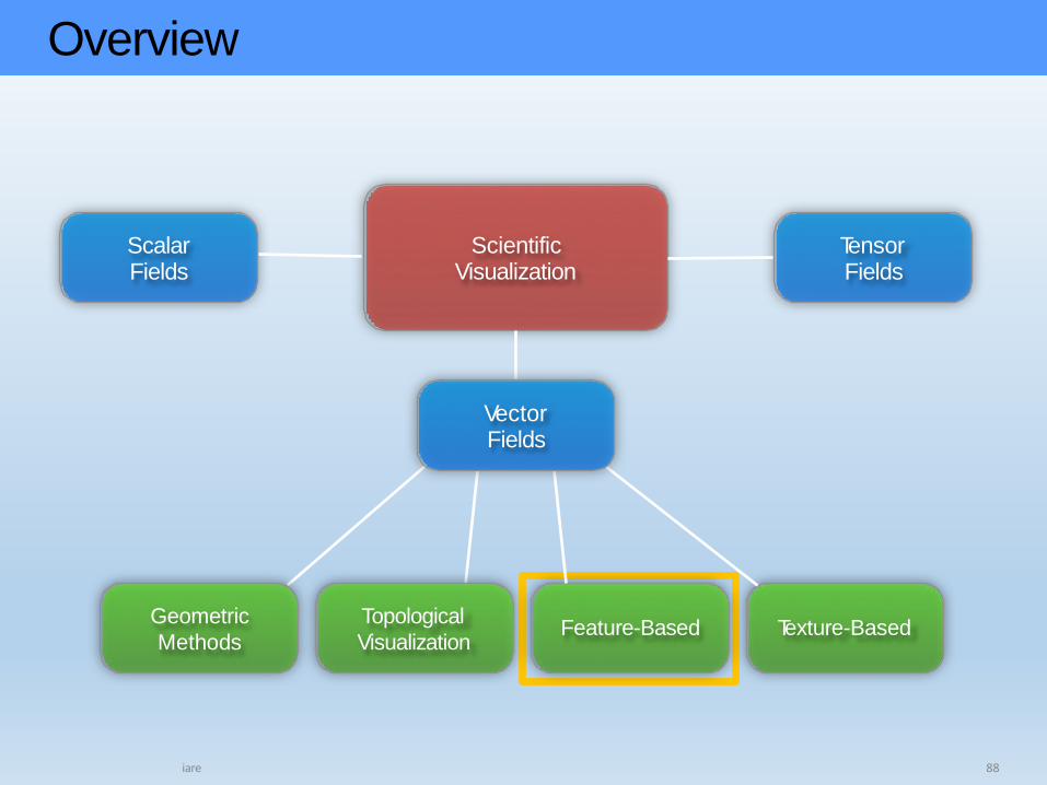
Overview
iare 88
Scientific Visualization
Tensor Fields
Scalar Fields
Geometric
Methods
Topological
VisualizationFeature-Based Texture-Based
Vector Fields

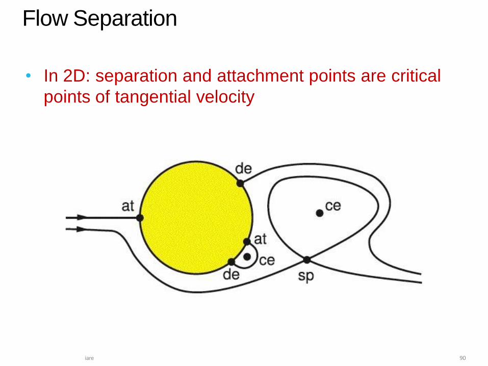
Flow Separation
iare 89
• Flow abruptly leaves or returns to solid body
(2D/3D phenomenon)
• Occurs along separation / attachment lines
Flow Separation
iare 90
• In 2D: separation and attachment points are critical
points of tangential velocity

Topological Approach
iare 91
• Work by Surana, Haller and others argue that flow
separation is indeed a topological structure

Flow Separation
iare 92

• Superimposition of wall streamlines
on oil flow patterns from experiment
Flow Separation
iare 93

• Kenwright̓s method: cell-wise pattern matching
• Basic observation: separation / attachment lines
present in two linear flow patterns
Flow Separation
iare 94
saddle node

• Kenwright̓s method: cell-wise patternmatching
• Idea: extract intersection of those lines with each cell in
piecewise linear flow
saddle
Flow Separation
iare 95
node

Flow Separation
96
FTLE over the Delta wing
iare
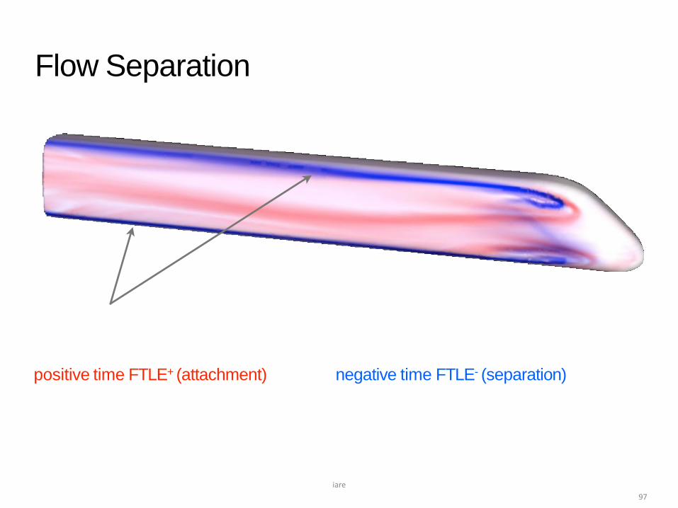
Flow Separation
97
positive time FTLE+ (attachment) negative time FTLE- (separation)
ICE trainvortex shedding
iare

Flow Separation
98
neighboring attachment/separation –
volume flow?
→ vortex
iare

Overview
iare 99
Scientific Visualization
Tensor Fields
Scalar Fields
Geometric
Methods
Topological
VisualizationFeature-Based Texture-Based
Vector Fields

• Spots of random intensity drawn and blended at random positions
Spot Noise
• General technique for synthesis of stochastic textures
• Texture is characterized by function f
iare 100
Scaling factor (random)
Spot function with local support
Random position
i
i if (x) = a h(x − x )
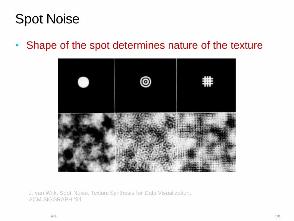
• Shape of the spot determines nature of the texture
J. van Wijk, Spot Noise, Texture Synthesis for Data Visualization, ACM SIGGRAPH ‘91
Spot Noise
iare 101

Spot Noise
iare 102
• Spot function allows for local control over texture:
maps data value (vector) to spot
J. van Wijk, Spot Noise, Texture Synthesis for Data Visualization, ACM SIGGRAPH ‘91

• Spot blending assumes local smoothness of underlying flow
field
Spot Noise
iare 103
• Elliptical spots for visualizing 2D flows
• Aligned with local flow direction
• Long axis proportional to v(x)
• Small axis proportional to 1/|v(x)
• Orthogonal to flow direction (waves)

• Animated Spot Noise for steady flow visualization:
• Spots as moving particles
• Over (fixed) lifetime
• Appears
• Moves along flow
• Decays
• Insertion position
• Insertion time
• Max intensity
Spot Noise
iare 104
random

• Spot bending (high flow curvature)
• Account for convergence divergence
• Ensure constant surface for each spot
• Solution: locally integrate stream surface
Enhanced Spot Noise
iare 105
W. de Leeuw, J. van Wijk, Enhanced Spot Noise for Vector Visualization, IEEE Visualization ‘95

Enhanced Spot Noise
iare 106
• Further improvements
• High-pass spot filtering to increase texture
homogeneity (avoid large light/dark regions)
W. de Leeuw, J. van Wijk, Enhanced Spot Noise for Vector Visualization, IEEE Visualization ‘95

Enhanced Spot Noise
iare 107
• Results
W. de Leeuw, J. van Wijk, Enhanced Spot Noise for Vector Visualization, IEEE Visualization ‘95

Line Integral Convolution
iare 108

Line Integral Convolution
iare 109
• Aliasing problems induced by white noise input texture can be solved by applying low pass filter (blurring) in pre-processing
• Simple convolution kernel: box
• Special convolution kernels can be used to show flow direction (periodic motion)
• Normalization applied after convolution to preserve brightness and contrast

Line Integral Convolution
iare 110
• Correlation of pixels along the flow
• No correlation orthogonal to the flow
• Resulting pictures are similar to visualizations
achieved with oil film applied onto surface of
embedded body in wind tunnel experiments
B. Cabral, C. Leedom, Imaging Vector Fields Using Line Integral Convolution, ACM SIGGRAPH ‘93

Line Integral Convolution
111
• Results
Standard LIC
iare

LIC
iare 112
• Results
LIC + color coded
flow magnitude

• Results
LIC
iare 113
LIC +
histogram equilization

• Results
LIC
iare 114
LIC +
high pass filter
FastLI
C
iare 115
• Exploit redundancy of streamlines covering many pixels
• # streamlines is 2% of # pixels
• Use correlation between convolution coefficients
• Integrate flow using RK 45 + cubic interpolation
• 10x faster than standard LIC
D. Stalling, H.-C. Hege, Fast and Resolution Independent Line Integral Convolution, ACM SIGGRAPH ‘95

• Improve contrast by iteratively taking last computed
LIC texture as input for next iteration
• Combined with final high-pass filtering
Enhanced LIC
iare 116
A. Okada, D. L. Kao, Enhanced Line Integral Convolution and Feature Detection, IS & T / SPIE Electronics Imaging ‘97

Oriented LIC
iare 117

Multifrequency LIC
iare 118
Kiu & Banks, Vis96
• Change frequency of noise texture
image based on flow properties (e.g
speed)

Moving Textures
iare 119
N. Max, B. Becker, Flow Visualization Using Moving Textures, Data Visualization Techniques, John Wiley & Sons, 1999
Vertices forward advection Backward texture advection Inverse flow

LEA
iare 120
B. Jobard, G. Erlebacher, M. Y. Hussaini, Lagrangian-Eulerian Advection of Noise and Dye Textures for Unsteady Flow Visualization, IEEE TVCG 8(3), 2002
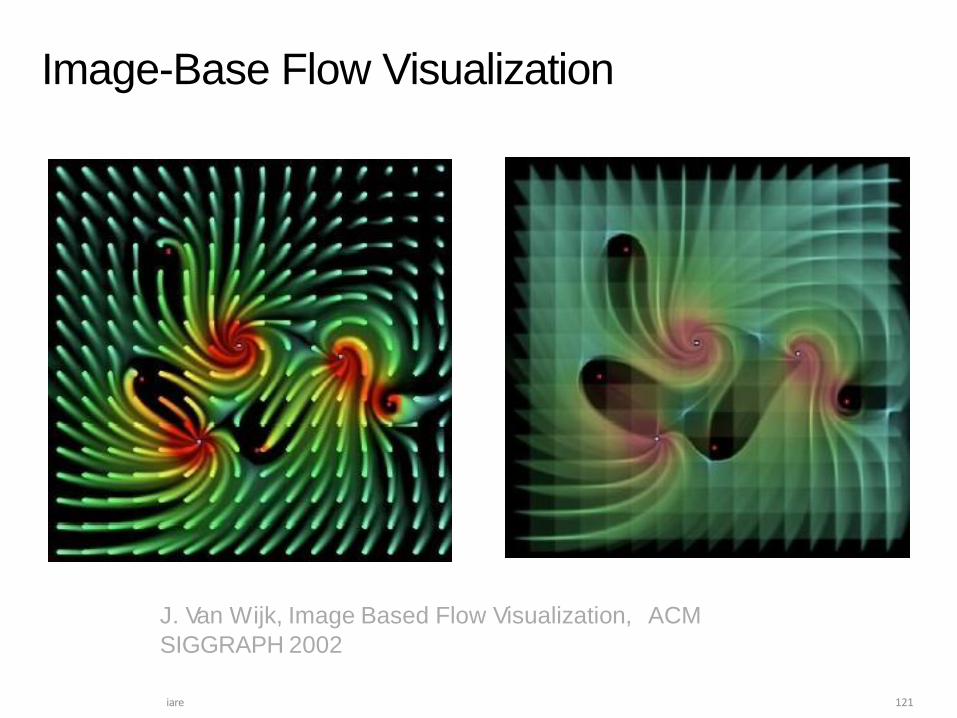
Image-Base Flow Visualization
iare 121
J. Van Wijk, Image Based Flow Visualization, ACM
SIGGRAPH 2002

IBFV
iare 122
J. Van Wijk, Image Based Flow Visualization, ACM
SIGGRAPH 2002

Unsteady LIC
iare 123
H.-W. Shen, D. Kao, A New Line Integral Convolution Algorithm for Visualizing Time-Varying Flow Fields, IEEE TVCG 4(2), 1998

iare 124
Top Related