


Languages
Pages
Legal


0
Asymmetric Volatility and the Cross-Section of Returns: Is Implied
Market Volatility a Risk Factor?
R. Jared Delisle
James S. Doran
David R. Peterson
Florida State University
Draft: June 6, 2009
Acknowledgements: The authors acknowledge the helpful comments and suggestions of Robert
Battalio, David Denis, Dirk Hackbarth, Chris Stivers, Ilya Strebulaev, Anand Vijh, Keith
Vorkink, David Yermack, and Jialin Yu. All remaining errors are our own.
Corresponding author: Jared Delisle
Department of Finance
College of Business
Florida State University
821 Academic Way, PO Box 3061110
Tallahassee, FL 32306
Email: [email protected]
0
Asymmetric Volatility and the Cross-Section of Returns: Is Implied Market Volatility a Risk
Factor?
ABSTRACT
Several versions of the Intertemporal Capital Asset Pricing Model predict that
changes in aggregate volatility are priced into the cross-section of stock returns.
Literature confirms this prediction and suggests that it is a risk factor. However,
prior studies do not test whether asymmetric volatility affects if firm sensitivity to
innovations in aggregate volatility is related to risk, or is just a characteristic
uniformly affecting all firms. We find that sensitivity to VIX innovations affects
returns when volatility is rising, but not when it is falling. When VIX rises this
sensitivity is a priced risk factor, but when it falls there is a positive impact on all
stocks irrespective of VIX loadings.

1
Introduction
Merton’s (1973) Intertemporal Capital Asset Pricing Model (ICAPM) implies that the
cross-section of stock returns should be affected by systematic volatility. Using a time-varying
model, Chen (2003) demonstrates that changes in the expectation of future market volatility are a
source of risk. Verifying this prediction, Ang, Hodrick, Xing, and Zhang (2006) find that
sensitivities to changes in implied market volatility have a cross-sectional effect on firm-level
returns. While Ang et al. show that the cross-sectional pricing of sensitivity to innovations in
implied market volatility is robust, it remains unclear if this sensitivity is a risk factor, or merely
a firm characteristic where there is a premium related to volatility risk just for being a stock. In
particular, Ang et al. do not account for the asymmetric return responses to positive and negative
changes in expected systematic volatility, as found by Dennis, Mayhew, and Stivers (2006).
Thus, the cross-sectional relation between sensitivity to market volatility innovations and firm
returns may not yet be fully understood. We extend prior studies by more fully documenting this
relation and testing for the presence of risk versus firm characteristics following procedures
developed by Daniel and Titman (1997), while allowing for asymmetric volatility responses. We
find that the asymmetric volatility phenomenon is an important element in the return process and
that firm sensitivity to innovations in implied market volatility is a priced risk factor when
implied market volatility rises, but not necessarily when it falls.
Identification of priced risk factors is at the core of asset pricing literature. However, the
identification of risks versus characteristics has proven to be a daunting task. The debate about
risk factors versus characteristics is important because it addresses the risk-return relation of
securities. Investors should be compensated for assuming higher systematic risk, but
characteristics are diversifiable and therefore should not be priced. In an efficient market,

2
loadings on risk factors should explain the cross-sectional variation in returns, and not
characteristics.
The ratio of book-to-market equity (B/M), size, and market beta are firm traits at the
center of the risk versus characteristic debate. Fama and French (1993) parse some
characteristics commonly used to explain stock returns and find that B/M proxies for common
risk factors. Davis, Fama, and French (2000) reach a similar conclusion, whereas Daniel and
Titman (1997) and Daniel, Titman, and Wei (2001), instead, find that B/M is a characteristic.
Lakonishok, Shleifer, and Vishney (1994) argue that the return premium for the B/M factor is
too high for it to be a measure of systematic risk. The size premium has also not been
definitively identified as a risk or characteristic. In fact, the formal tests on size performed by
Daniel and Titman and Davis, Fama, and French find evidence that supports both risk-based and
characteristic-based pricing processes. Additionally, there is little support for market beta as a
measure of risk. Fama and French (1992, 1993) and Daniel and Titman find that there is a
premium over the risk-free rate for being a stock, but the covariance of a stock’s return with the
market is irrelevant.
Another aspect of the returns process that has been examined, but is also subject to
individual interpretation, is the sensitivity of stock returns to aggregate volatility. Through their
variations of Merton’s (1973) ICAPM, Campbell (1993, 1996) and Chen (2003) demonstrate that
investors can interpret a market volatility increase as a decrease in their set of investment
opportunities. Chen’s model shows that a decrease in expectation of future market volatility
allows investors to decrease precautionary savings and increase consumption. Conversely, an
increase in expected future market volatility produces a decrease in consumption and an increase
in precautionary savings, resulting in price declines. Thus, risk-averse investors should hedge

3
against changes in future volatility by acquiring stocks that are positively correlated with
aggregate volatility innovations. Investors choose the stocks that are positively correlated with
changes in market volatility because market returns and market volatility are negatively
correlated. Bakshi and Kapadia (2003) note that due to the negative correlation between returns
and volatility, stocks that load heavily on market volatility provide insurance against downward
market movements. The demand for such stocks drives up their prices contemporaneously, and
thus lowers their future returns. This reasoning suggests that the pricing of sensitivity to market
volatility is risk-based.1
Prompted by these implications that exposure to market volatility changes can result in
cross-sectional differences in returns, Ang, Hodrick, Xing, and Zhang (2006) investigate if
sensitivity to systematic volatility is cross-sectionally priced. They employ the VIX index and a
factor portfolio that mimics innovations in the VIX index. They first difference the VIX index
since, as Chen points out, investors react to the changes in expected market volatility, as well as
to avoid any serial correlation in the index.2 Ang et al. obtain loadings on changes in VIX,
henceforth denoted VIX, sort the stocks into quintile portfolios monthly based on their
loadings, and examine the portfolio returns in the following month.
The quintile portfolios show a monotonic decrease in future value-weighted returns as the
loadings increase, and the difference in the returns of the extreme quintile portfolios are
significantly different from each other. In concordance with the predictions of Merton (1973),
Campbell (1993, 1996), and Chen (2003), these empirical findings indicate that there is a
1 However, studies of the time-series relation between market volatility and market returns by French, Schwert, and
Stambaugh (1987), Campbell and Hentschel (1992), Glosten, Jagannathan, and Runkle (1993), and Wu (2001) are
ambiguous about if market volatility is a priced risk factor in the cross-section of stock returns. 2 Ang et al. find that their results are robust to measuring volatility innovations in an AR(1) model of VIX, as well as
a model using an optimal number of autoregressive lags as specified by the Bayesian Information Criteria (BIC).

4
negative premium associated with the sensitivity to innovations in market volatility. Investors
appear to pay more for securities that do well when volatility risk increases; thus, the high-
loading firms have lower future returns than the low-loading firms. Ang et al. conclude that the
sensitivity to innovations in implied market volatility is a priced risk factor after showing the
results are robust to matching firm returns from one of the Fama and French (1993) 25 size and
B/M portfolio returns and after controlling for liquidity, volume, and momentum.
Ang et al. provide preliminary evidence that aggregate volatility sensitivity is cross-
sectionally priced; however, their tests are incomplete for three reasons. First, they present
incomplete results about whether the pricing of sensitivity is actually risk-based or characteristic-
based. All reported zero-cost portfolio returns have both means and Fama and French (1993)
three-factor alphas that are significantly different from zero, which suggests a risk-based pricing
kernel. But if expected market volatility is a priced risk factor and the sole explanation for
returns of portfolios differing only in loadings, then the incorporation of volatility innovations as
an additional explanatory variable into an augmented factor model should produce alphas
indistinguishable from zero. While Ang et al.’s focus is not on this issue, the implications of
their findings lead us to test a broader, more robust specification.
Second, more powerful tests can be made by grouping stocks into portfolios of like
characteristics prior to examining the sensitivities to volatility changes. The portfolios formed in
Ang et al. are not initially size and B/M characteristic-balanced, possibly confounding tests of a
risk versus characteristic pricing process. Additionally, alphas from the size and B/M matching
analysis performed by Ang et al. are unreported, so it is not clear if loadings matter after
controlling for the Fama and French factors.
5
Third, and most important, the model used by Ang et al. to obtain loadings on volatility
changes assumes a symmetric relation between returns and innovations in implied market
volatility. Significant literature, however, shows there is an asymmetric volatility phenomenon
where positive returns are associated with smaller changes in implied volatilities than negative
returns of the same magnitude.3 Specifically, Dennis, Mayhew, and Stivers (2006) examine the
relation between stock returns and VIX allowing for stock returns to react asymmetrically to
volatility shocks.4 Their goal is to determine if the asymmetric volatility phenomenon stems
from systematic or idiosyncratic effects. While not directly testing for a risk-return relation, they
find that firm-level returns have a much stronger relation with changes in market-level implied
volatility than with innovations in implied idiosyncratic volatility. Their findings suggest that
the asymmetric volatility phenomenon at the firm level is very much related to systematic
effects. The relation to systematic effects means that sensitivities to VIX innovations may be
cross-sectionally priced with different relations for upward and downward innovations; firm-
level returns should react differently in magnitude to a positive innovation in VIX than to a
negative innovation in VIX.
Consequently, the specification used by Ang et al. may only capture a mean loading that
is not sensitive to the state of VIX. This can be an important omission, since the degree of
asymmetry of the loading can place a stock into an incorrect quintile ranking if the asymmetry is
ignored. The asymmetric volatility phenomenon may be why Ang et al. find that the average
turnover in their monthly quintile portfolios is above 70%; the mean-reversion property of VIX
suggests that a period of upward movements will be followed by downward movements and
3 See Bekaert and Wu (2000) and Wu (2001) for asymmetric volatility models and literature review. 4 Adrian and Rosenberg (2008) employ an asymmetric volatility model to examine short- and long-run effects of
market volatility on the cross-section of stock returns, but use historic volatility rather than the VIX index.

6
stocks with asymmetric relations to changes in VIX may migrate to different portfolios
depending on the degree of asymmetric relations. Ang et al. find that the longer their formation
window, the smaller the spread in pre-formation loadings on VIX. Ignoring the asymmetric
relation could cause this outcome because as more observations enter the window, the more
equal are the number of positive and negative innovations in VIX. Thus, the loadings on VIX
changes would move toward an average of loadings on positive innovations and loadings on
negative innovations.
We build on the findings of Ang et al. (2006) and Dennis et al. (2006). We examine the
effect of sensitivities to implied market volatility on portfolio returns by modeling the return
process as a function of the innovations in the VIX index, allowing for asymmetric reaction to
implied market volatility. Portfolios are formed by sorting the sample into nine size and B/M
portfolio bins. We then use a Daniel and Titman (1997) approach to discern if the
contemporaneous relation is risk or characteristic based. The stocks in each size and B/M bin are
sorted according to their loadings on VIX and characteristic-balanced, zero-cost portfolios are
created by buying stocks that load high on VIX and selling stocks that load low on VIX. The
portfolios are considered characteristic-balanced since all stocks in a portfolio have the same size
and B/M characteristics, and any contemporaneous differences in the returns in the long-short
portfolios can be attributed to their different loadings on VIX. Therefore, if the mean returns of
the zero-cost portfolios and alphas from the traditional three-factor model (without volatility
innovations included) are significantly different from zero, and the alphas from the Fama and
French (1993) three-factor model augmented with VIX are not significantly different from
zero, then the risk-based process is accepted as the correct pricing model. If the characteristic
model is correct, then mean returns for the zero-cost portfolios will be zero.
7
For each security we estimate two different loadings on monthly VIX innovations,
conditional on whether the innovations are positive or negative. We apply the appropriate
loading to a given future month conditional on whether that month has a positive or negative
VIX innovation, and form five portfolios in that month based on ranked loadings. We examine
portfolio returns in the same month and, thus, returns are examined in a contemporaneous setting
with VIX innovations. Our framework is not intended to be predictive, but merely to illustrate
the contemporaneous risk-return relation, where that relation is allowed to conditionally change
depending on whether VIX increases or decreases.
Our analysis can be directly related to the risk-based hypotheses in Ang et al (2006).
They argue that the inverse relation between market volatility change loadings and the next
period’s returns reflects investors paying a premium (resulting in lower expected returns) for
stocks with high sensitivities to market volatility changes because they like stocks with relatively
high payoffs when volatility increases. In our model this will lead to an increase in market
volatility contemporaneously associating with high volatility loading stocks outperforming low
volatility loading stocks. When VIX declines, however, our model suggests that low volatility
loading stocks outperform high volatility loading stocks. Thus, our predicted risk-return relation
will be conditional on whether VIX rises or falls. By analyzing markets when VIX increases
separately from when it decreases, we are also able to explicitly incorporate asymmetric
volatility effects.
For the size and B/M characteristic-balanced portfolios, when there are positive
innovations in VIX, contemporaneous returns across the nine portfolios are negative, as
8
expected. They also have significantly negative three-factor alphas.5 When there are negative
innovations in VIX, contemporaneous returns across the nine portfolios are strongly positive and
three-factor alphas are significantly positive. These results suggest that VIX innovations affect
returns and the relation differs depending on whether VIX increases or decreases.
For the characteristic-balanced zero-cost portfolio returns, when there are positive
innovations in VIX, firms with high loadings on VIX significantly outperform those with low
loadings. Three-factor alphas are significantly positive, while alphas for a three-factor model
augmented with VIX are generally indistinguishable from zero. Since there are a few
significant alphas, however, hints of some unexplained effects in the augmented model remain.
Overall, these results tend to favor a risk-based explanation over a characteristic-based
explanation; they are also consistent with the results in Ang et al. When there are negative
innovations in VIX, firms with high loadings on VIX perform similarly to firms with low
loadings. Three-factor and augmented three-factor alphas are indistinguishable from zero. For
negative innovations in VIX, these results are not consistent with a risk story. Instead, as VIX
falls there is a contemporaneous strong positive effect on stock returns that influences different
stocks about the same. In other words, there is a premium just for being a stock. If a risk
explanation existed when VIX declines, the low-loading portfolio should contemporaneously
outperform the high-loading portfolio. Our above results are robust to liquidity, momentum,
price, volume, and leverage. They are also robust to cross-sectional firm-level Fama and
MacBeth (1973) regressions. Ultimately, our findings show that investors only care about
loadings when there are increases in implied market volatility.
5 As developed in the methodology section, in our three-factor model the traditional market factor is replaced by a
market factor orthogonalized to changes in VIX.
9
Our primary focus is on VIX since the VIX index is used for many purposes in finance,
is readily observable, and is a tradable asset. Also, Dennis et al.’s finding that innovations in the
VIX index are significant in predicting future realized index volatility make VIX a useful and
prudent proxy for changes in expected future market volatility. However, we repeat our analyses
using Ang et al.’s factor mimicking portfolio, FVIX, as the proxy for changes in aggregate
volatility in place of VIX.6 Our results are generally similar as to when we use VIX, with a
small difference for the zero-cost portfolios when FVIX is negative. Then, unlike with VIX,
zero-cost low-loading portfolios significantly outperform high-loading portfolios and two of nine
three-factor alphas are significantly different from zero. These results when FVIX is negative
may suggest a minor role for a risk-based explanation, whereas there is none when VIX is
negative.
The paper is developed in the following sections. Section I describes the data. Section II
explains the methodology and models. Section III presents the empirical results for VIX.
Section IV provides robustness results using FVIX. Section V concludes the paper.
I. Data
The sample is from January 1986 through December 2007. Monthly VIX index levels
are from the Chicago Board Options Exchange (CBOE) website, from which VIX is calculated.
The VIX index represents the implied volatility of a synthetic, at-the-money option on the S&P
6 We construct FVIX similar to Ang et al (2006).
10
100 index with 30 days to expiration.7 The VXO index (the predecessor to VIX that uses a
slightly different computational methodology) is used in place of VIX from 1986 through 1989.
Stock prices, monthly returns, and share volume are from the Center for Research in Security
Prices (CRSP), as are the value-weighted CRSP index returns. Only stocks with CRSP share
codes 10, 11, and 12 are kept in the sample. The share volumes for NASDAQ stocks are divided
by two to adjust for double-counting trades. The market risk premium (MKT), Fama and French
(1993) size and book-to-market factors (SMB and HML), risk-free rate, and NYSE size
breakpoints are provided by Ken French’s website.8
COMPUSTAT provides data for book equity and leverage. Book equity is the value of
stockholders’ equity plus all deferred taxes and investment tax credit, minus the value of any
preferred stock. The book-to-market equity ratio assigned to a firm from July of year to June
of year +1 is the book equity at the end of the fiscal year in calendar year -1 divided by the
market capitalization at the end of December of year -1. Similarly, leverage in year is defined
as the value of the total assets of the firm divided by the book equity, where both total assets and
book value of equity are calculated at the end of the fiscal year in calendar year -1. Only firms
with positive book equity are kept in the sample. In order to avoid any COMPUSTAT firm bias,
firms with less than two years of data on COMPUSTAT are removed from the sample. Pastor
and Stambaugh (2003) liquidity factors are from Wharton Research Data Services (WRDS).
Panel A in Table I shows the simple correlations between MKT, SMB, HML, VIX, and
the factor-mimicking portfolio FVIX, similar to that employed by Ang et al. (2006).9 MKT is
7 The construction of the VIX index is detailed by Whaley (2000) and also in a white paper available at the CBOE’s
website: http://www.cboe.com/micro/vix/vixwhite.pdf. 8 Ken French’s website is located at http://www.dartmouth.edu/~kfrench/. 9 The construction of FVIX and results from its use are discussed later.
11
highly negatively correlated with VIX and FVIX. Panels B and C report the correlations
conditional on whether MKT is positive or negative. These two panels demonstrate the nature of
the asymmetric volatility phenomenon. The negative correlations of VIX and FVIX with
market returns are substantially larger in magnitude when MKT is negative (-0.6981 and -
0.7197, respectively) than when it is positive (-0.1808 and -0.2681, respectively). These
correlations, however, are just simple correlations, and there are occasions when market returns
and VIX are positively correlated. In 31 percent of the observations MKT has the same sign as
VIX; in two-thirds of these observations MKT and VIX are both positive and in the remaining
one-third they are both negative.
II. Methodology
A. Construction of Adjusted Factor Loadings on VIX
The first step to empirically obtain adjusted factor loadings is to regress individual
monthly stock returns, in excess of the risk-free rate, on VIX and an interaction term composed
of VIX times a dummy variable reflecting if VIX is positive or not. The interaction term
allows for an asymmetric relation between returns and changes in implied market volatility,
allowing for a different response to positive and negative innovations in VIX. This regression is:
𝑟𝑖,𝑡 = 𝛼𝑖 + 𝛽∆𝑉𝐼𝑋 ,𝑖∆𝑉𝐼𝑋𝑡 + 𝜃𝑖𝑃𝑂𝑆𝑡∗∆𝑉𝐼𝑋𝑡 + 𝜀𝑖,𝑡 (1)
where ri,t is the excess return for firm i in month t, VIXt is the innovation in VIX from the end
of month t-1 to the end of month t, POSt is a dummy variable that equals one in months when
VIX is positive and zero otherwise, and i,t is an error term. This regression is estimated for
12
each firm for June of year over 54 months ending in December of year -1. We require at least
36 months of data and, thus, the earliest regressions end in December, 1988. The beta and theta
estimates for each June of year are assigned to July of year through June of year +1.
Although each firm’s parameter estimates are held constant for twelve-month periods,
they are used to create adjusted factor loadings (AFL’s) for VIX innovations each month using
the realized value of POSt for each respective month from July of year through June of year
+1. The computation of AFL’s is:
𝐴𝐹𝐿∆𝑉𝐼𝑋 ,𝑖 ,𝑡 = 𝛽 ∆𝑉𝐼𝑋 ,𝑖 + 𝜃 𝑖𝑃𝑂𝑆𝑡 (2)
where AFLVIX,i,t is the AFL representing the marginal effect of VIX for the returns of stock i
for month t. For example, the regression may be estimated for one firm over 54 months from
June, 2001, to December, 2005, and the resulting parameter estimates (𝛽 ∆𝑉𝐼𝑋 and 𝜃 ) for June,
2006, are assigned to the firm from July, 2006, through June, 2007. The AFL for July, 2006,
uses the assigned parameter estimates and the POS dummy value (0 or 1) corresponding to the
sign of VIX that is realized for July, 2006. The AFL’s for August, 2006, through June, 2007,
are similarly calculated, using the same 𝛽 ∆𝑉𝐼𝑋 and 𝜃 used for the AFL computation in July, 2006,
but using the respective POSt for each month. The analysis begins with July, 1988.
B. Portfolio Formation
Each month we sort the stocks into quintiles based on the VIX AFL’s. This method of
portfolio formation is common to the size and book-to-market sorts of Fama and French (1993)
and Daniel and Titman (1997). The important difference comes from the inclusion of the
13
interaction term in the regression, which allows each firm to have an asymmetric relation with
VIX, and ensures that the firms are placed into quintile portfolios subject to the realization of
the direction of VIX. If the asymmetric relation is large enough, the stock may change quintile
portfolios depending on whether VIX is positive or negative. If this is the case for a given
stock, then the stock can be in one of two portfolios during the 12-month period that the
parameters estimates are held constant, one portfolio when VIX is negative and another when
VIX is positive. Ang et al.’s (2006) average VIX loadings of the post-formation portfolios
are not well dispersed and this could be due to the lack of accounting for the asymmetric
volatility phenomenon. Much of our analysis is based on zero-cost portfolios formed from
differences in returns between the fifth and first quintiles.
Similar to Daniel and Titman (1997), we initiate our pricing model tests by sorting the
sample into size terciles based on NYSE breakpoints, and then sequentially sorting into book-to-
market equity (B/M) terciles. The sorts are performed sequentially in order to guarantee that the
number of stocks in each size-B/M bin is sufficiently large. The size of the firm is determined in
June of calendar year and assigned to the firm from July of calendar year to June of year +1.
The B/M of each firm is determined by the book value at the fiscal year-end in calendar year -1
divided by the market capitalization of the firm at the end December of year -1 and assigning it
to the firm from July of calendar year to June of calendar year +1. This sorting procedure
leads to nine separate size and B/M portfolio bins and in each bin the stocks have similar size
and B/M characteristics, or are characteristic balanced. We analyze the returns of these
portfolios both when VIX rises and when it falls.
14
Next, in each portfolio bin the stocks are divided into equal quintiles based on the pre-
formation AFL’s. Following Daniel and Titman (1997), we construct zero-cost characteristic-
balanced portfolios, that differ only in AFL’s, by buying stocks in the fifth quintile (loading the
highest on VIX) and selling the stocks in the first quintile (loading the lowest on VIX) in each
size-B/M bin. This procedure is done both for months when VIX rises and when it falls.
A characteristic-based returns model predicts that the returns of the five portfolios in each
size-B/M bin will not be significantly different from each other, since they all share the same
characteristics and loadings on VIX do not matter. Conversely, a risk-based model predicts
that in each size-B/M bin the stocks with high loadings on VIX will have different mean returns
than the low-loading stocks. This prediction reflects that, among stocks that have similar
characteristics, it is the AFL’s that generate cross-sectional differences in returns. Also, if cross-
sectional differences in returns due to AFL’s are risk-based with no residual unexplained
components, then the alphas from the Fama and French (1993) three-factor model, augmented
with VIX, should be zero since the model explains all the risk components of portfolio returns.
We use two variations of the Fama and French (1993) three-factor model to estimate
abnormal returns, or alphas. The difference between the two models is if VIX is included as an
independent variable. Expectations of market volatility may substantially affect market returns
and MKT in the traditional three-factor model. To isolate the effect of VIX on portfolio
returns, we orthogonalize MKT to VIX. We consider this essential to remove the effect of
volatility from MKT. As seen in Heston (1993) and others, volatility follows a stochastic, mean-
reverting process. The form of the discrete price and volatility processes are:
∆𝑆𝑡
𝑆𝑡= 𝜇∆𝑡 + 𝑉𝑡∆𝑊𝑠 (3)
15
∆𝑉𝑡 = 𝑘 𝜃 − 𝑉𝑡 ∆𝑡 + 𝜎 𝑉𝑡∆𝑊𝑣 (4)
where St is the equity spot price at time t, Vt is the variance of equity spot price at time t, is the
rate of drift of the equity spot price, k is the rate of mean reversion of the variance, is the long
run mean of the variance, is the volatility of the variance, and Ws and Wv are standard Wiener
processes that are correlated by such that
∆𝑊𝑠 ∙ ∆𝑊𝑣 = 𝜌∆𝑡 (5)
Note that the returns process (equation (3)) is explicitly a function of the variance (Vt) as well as
implicitly a function of the variance through the correlation of the two Wiener processes
(equation (5)). The variance process (equation (4)), however, is only influenced by the returns
process through correlation of the Wiener processes. This is the motivation for orthogonalizing
MKT to VIX, and not vice versa.
We orthogonalize the traditional market factor to changes in VIX by regressing MKT on
VIX and using the residual in month t plus the intercept to form MKT⊥. By orthogonalizing
MKT to VIX, we remove the expected market variance component from the market returns and
isolate it in VIX. MKT is decomposed into two parts, that due to market volatility innovations
and an uncorrelated residual plus intercept component. We also orthogonalize MKT because it
is highly negatively correlated with VIX, as shown in Table I. The coefficient on MKT⊥ thus
measures the effect on returns from the portion of the market factor unrelated to VIX.
We then estimate the two variations of the traditional Fama and French (1993) three-
factor model as:
16
𝑟𝑝 ,𝑡 = 𝑎𝑝 + 𝛽𝑀𝐾𝑇 ,𝑝𝑀𝐾𝑇𝑡⊥ + 𝑠𝑝𝑆𝑀𝐵𝑡 + ℎ𝑝𝐻𝑀𝐿𝑡 + 𝜀𝑝 ,𝑡 (6)
and 𝑟𝑝 ,𝑡 = 𝑎𝑝 + 𝛽𝑀𝐾𝑇 ,𝑝𝑀𝐾𝑇𝑡⊥ + 𝑠𝑝𝑆𝑀𝐵𝑡 + ℎ𝑝𝐻𝑀𝐿𝑡 + 𝛽∆𝑉𝐼𝑋 ,𝑝∆𝑉𝐼𝑋𝑡 + 𝜀𝑝 ,𝑡 (7)
III. VIX Results
A. Cross-Sectional Portfolio Returns and VIX
The characteristics of the quintile portfolios single-sorted by AFL’s on VIX are reported
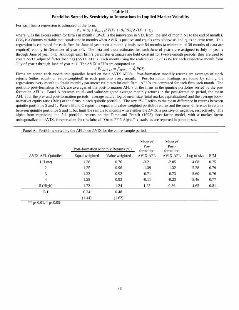
in Panel A of Table II. The sort produces smaller firms in the lowest and highest quintiles. The
lowest quintile portfolio based on VIX AFL’s sorts has a slightly lower B/M than the other
portfolios. Overall, the B/M ratios for the five portfolios are very similar.
The pre-formation loadings are used to predict post-formation loadings. If the loadings
are not stable through time, then tests are not reliable since the post-formation portfolios will not
be ranked correctly. Post-formation loadings are obtained by performing the regression
described in equation (1) for each firm, and rolling the regressions forward every month to obtain
monthly parameter estimates for each firm in each month. Equation (2) is used to form the
AFL’s for each firm each month. The portfolio post-formation AFL’s are averages of the post-
formation AFL’s of the firms in the quintile portfolios sorted by the pre-formation AFL’s. After
the single-sort quintile portfolios are formed, the post-formation loadings are examined to see if
the loadings are stable through time. As shown in Panel A of Table II, the portfolios sorted on
AFL’s maintain a good dispersion in the mean post-formation AFL’s that is very similar to the
mean pre-formation AFL’s. Ang et al. (2006) find poor dispersion in the mean post-formation
loadings when sorting on pre-formation loadings on VIX. However, their study focuses on the
17
portfolio returns in the month following portfolio formation, while our study focuses on the
contemporaneous returns with asymmetric volatility.
Concerned that VIX may include components other than diffusion risk (such as jump
risk and/or a stochastic volatility risk premium), Ang et al. (2006) create the factor-mimicking
portfolio FVIX, replace VIX with FVIX in their original regression relating returns to changes
in implied market volatility, and find that the average FVIX loadings of portfolios sorted by
VIX loadings are well-dispersed. We repeat all analyses with FVIX, calculated as in Ang et al.,
and present these results in our robustness section.
In a manner similar to Ang et al., we first present results before forming size and B/M
sorted portfolios. Equal and value-weighted returns are computed for the five quintiles of VIX
AFL’s and reported in Panel A of Table II. There are slight increases in returns from the low to
the high quintiles of AFL’s. As discussed in the introduction, this is not contradictory to Ang et
al.’s results since our table presents returns that are contemporaneous to the formation of AFL
quintile portfolios and incorporate asymmetric volatility in the formation of the AFL’s. Note
that only the stocks in the highest AFL quintile have positive average AFL's. Since VIX and
market returns are negatively correlated, as seen in Table I, this is an expected result.10
A
positive loading on VIX is akin to a negative loading on the market risk premium, which is
unusual. This property of the stocks in the fifth quintile makes them attractive as hedging
10 The negative correlation between market returns and volatility is documented by French, Schwert, and Stambaugh
(1987) and Campbell and Hentschel (1992).
18
instruments.11
The AFL’s indicate that returns on this quintile of stocks increases as market
volatility increases. It is likely that only a small percentage of stocks would exhibit this property.
Panel A of Table II shows that a zero-cost portfolio of going long quintile five stocks and
shorting quintile one stocks (hereafter such a portfolio is called a 5-1 portfolio) yields returns
insignificantly different than zero. This result is expected. VIX has a mean close zero, with
about an equal number of positive and negative realizations. Because the average AFL in
quintile one is negative and the average AFL in quintile five is positive, we expect that a 5-1
portfolio return will be positive when VIX is positive and negative when VIX is negative.
Thus, a simple t-test of mean returns on a 5-1 portfolio can be inconclusive due to the
aggregation of the positive and negative portfolio returns resulting in a mean return close to zero.
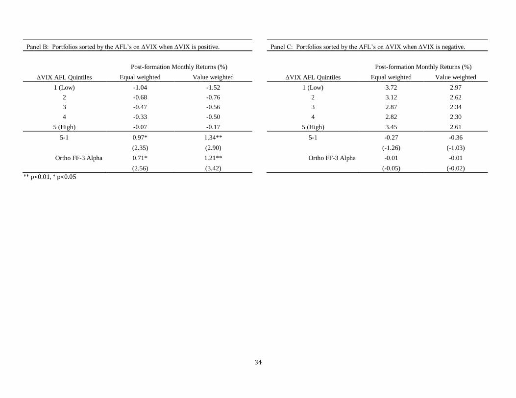
In Panels B and C of Table II, the equal- and value-weighted returns of the 5-1 portfolios
are tabulated conditional on the contemporaneous VIX. When VIX is positive, the ten sorted
portfolios have monthly negative returns that are close to zero for high-loading firms and range
to -1.52% for low-loading firms. The 5-1 portfolios have statistically significant positive returns
and the three-factor model with MKT⊥, SMB, and HML has significant alphas, suggesting that
loadings matter and that a risk explanation may apply when VIX rises. When VIX is negative,
all ten sorted portfolios have monthly returns of at least 2.30%. There is little return discrepancy
across the portfolios and the 5-1 returns and alphas are statistically insignificant. These results
are not conducive to a risk explanation as loadings do not matter. Instead, there is a strong
positive return to all stocks, irrespective of loadings, when VIX falls. The results in Panels B
and C highlight the importance of asymmetric volatility.
11 This point is also made by Bakshi and Kapadia (2003), Ang et al. (2006), Dennis et al. (2006), and Adrian and
Rosenberg (2008).
19
The results thus far show that there is a relation between VIX loadings and the cross-
section of stock returns. In order to establish that the AFL’s on VIX are stable through time
within the nine size and B/M bins from tercile sorting, we examine the pre- and post-formation
AFL’s for the entire sample and conditional on the direction of VIX. These results are reported
in Table III. The pre-formation AFL’s on VIX are well dispersed, and the rankings and
dispersion hold for post-formation AFL’s. The average pre-formation (post-formation) AFL’s
are -1.00 and -0.96 (-1.04 and -0.99) for small and medium-size growth firms, respectively,
which are more negative than those of the other size and B/M bins, which range from -0.67 to -
0.79 (-0.69 to -0.80).
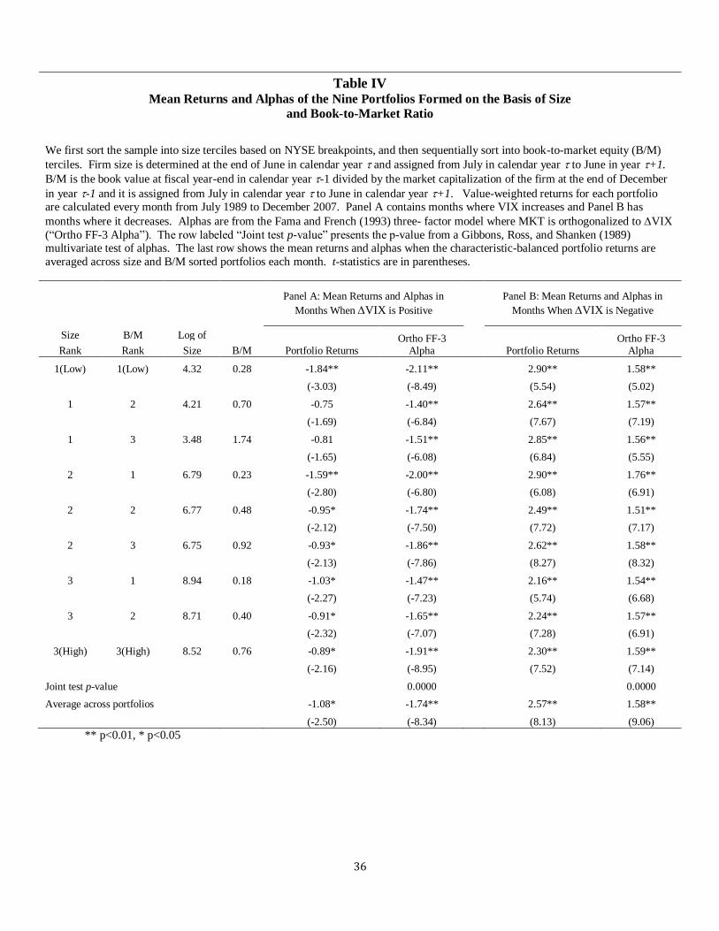
Panels A and B of Table IV present value-weighted returns for the nine size and B/M
sorted portfolios from periods when VIX is positive and negative, respectively.12
When VIX
increases, all nine portfolios have significantly negative returns and three-factor alphas. A
Gibbons, Ross, and Shanken (1989) multivariate test of the alphas shows that they are jointly
highly significant. For characteristic-balanced portfolios, VIX increases negatively impact
returns and this effect is not reduced in a factor model with MKT⊥, SMB, and HML included.
The three-factor alphas are more negative and strongly significant than the raw returns. When
VIX decreases, all nine portfolios have positive and highly significant returns and three-factor
alphas. The multivariate test of the alphas shows that they are jointly highly significant. The
absolute values of returns are larger than when VIX increases, although the three-factor alphas
are not. Thus, for characteristic-balanced portfolios, VIX decreases positively impact returns in
12 Unreported results show that across all subsequent analyses, equal-weighted returns provide quantitatively and
qualitatively similar findings to that of the value-weighted returns.
20
a strong manner, though a little less than half the impact is eliminated in a factor model with
MKT⊥, SMB, and HML included.
B. The Impact of Asymmetric Volatility on VIX as a Risk Factor
We next examine returns for the nine portfolios, where each is divided into five portfolios
based on AFL’s. Panel A of Table V presents results for months when VIX rises and Panel B
has results for months when VIX falls. When VIX rises, all nine 5-1 returns are positive and five
of the nine are significantly different from zero at the 5% level or better. All alphas from the
three-factor model with MKT⊥, SMB, and HML are positive, with eight significant at the 5%
level or better. They are similar in size to the 5-1 returns, and the joint alpha test is significant at
the 1% level. Significant three-factor alphas show the inability of the model to capture all the
risk contained in the portfolios and, in an efficient market, suggest there is risk present other than
that captured by MKT⊥, SMB, and HML. The average 5-1 return and alpha effects across
portfolios are 25%-35% below the corresponding value-weighted numbers in Table II, Panel B.
This highlights the importance of forming characteristic controlled portfolios. The three-factor
model augmented with VIX innovations has eight of nine individual alphas insignificantly
different than zero, and the joint test of significance cannot reject the null hypothesis of alphas
equal to zero. Although only one is significant, typical augmented model alphas retain about
one-half the value of the three-factor alphas and raw returns.
All of these results suggest that when VIX rises, factor loadings matter, consistent with
the conclusion that VIX innovations represent a priced risk factor. Zero-cost characteristic-
balanced portfolios can be constructed, albeit based on ex-post information, that generate both
21
statistically and economically significant mean returns. But since these returns can be explained
by a model that includes VIX innovations, VIX appears to be a risk factor. The sensitivity to
changes in implied market volatility has a cross-sectional effect on stock returns that follows a
risk-based returns process, and this risk is not captured by the three-factor model. However, an
augmented model that incorporates VIX seems to explain most of the return. There is, perhaps,
a hint of some residual return left over that is captured in the augmented model alphas, which
may suggest part of the 5-1 returns cannot be explained by the four factors in the model.
When VIX falls, all nine 5-1 returns are negative, but none are significant. None of the
alphas are significant either. These results are not consistent with a risk story; loadings do not
matter. Instead, all portfolios have similar returns that are quite high, ranging from 2.14% to
3.55% per month. These results, consistent with those in Table II, suggest that when VIX falls,
there is a large positive premium for the characteristic of being a stock, with no differentiation
based on loadings. All stocks rise substantially and similarly when VIX falls.
C. Effects of Other Firm Characteristics on the Role of VIX
We next examine if the previous results are robust to liquidity, momentum, price,
volume, and leverage. In order to get loadings on the Pastor and Stambaugh (2003) liquidity
factor (LIQ), a rolling regression is estimated (in a similar manner to equation (1)) as:
𝑟𝑖,𝑡 = 𝛼𝑖 + 𝛽𝑖𝑀𝐾𝑇𝑡 + 𝑠𝑖𝑆𝑀𝐵𝑡 + ℎ𝑖𝐻𝑀𝐿𝑡 + 𝑙𝑖𝐿𝐼𝑄𝑡 + 𝜀𝑖 ,𝑡 (8)
The regression is estimated over 54 months ending in December of year -1 with at least 36
months of data required. The loadings are assigned to stock i from July of year to June of year
22
+1. The stocks are sorted into quintile portfolios based on their loadings on LIQ. Six (twelve)
month momentum is constructed for each firm in June of year by accumulating the monthly
returns from December (June) of year -1 to April of year .13
The accumulated returns are
assigned to stock i from July of year to June of year +1, and the stocks are sorted into quintile
portfolios based on their six (twelve) month momentum. The quintile portfolios based on stock
price are created by sorting at the end of June of year and assigning the rankings from July of
year to June of year +1. To control for volume effects, firms are sorted into quintiles based on
the dollar trading volume over June of year and the rankings are assigned from July of year to
June of year +1. We define leverage as the ratio of the total book value of assets to the total
book value of equity at the fiscal year end occurring in calendar year -1. Firm leverage ratios
are sorted into quintiles and the rankings assigned from July of year to June of year +1.
In a manner similar to our original sorting procedure, a 3x3x3 triple sort is performed
every 12 months involving each of the robustness characteristics. The first sort is on size, the
second on B/M, and the third on the respective characteristic. Thus, we form 27 characteristic-
balanced portfolios. Next, in each portfolio bin the stocks are divided into equal quintiles based
on the pre-formation AFL’s. As before, we construct zero-cost characteristic-balanced portfolios
in each bin, differing only in AFL’s, by buying stocks in the fifth quintile and selling the stocks
in the first quintile. This is done both for months when VIX rises and when it falls. Each month
the value-weighted returns of the zero-cost portfolios are computed and averaged across the 27
bins.14
This average return is used in the regressions.
13 Jegadeesh and Titman (1993) document the momentum effect. 14 Equal-weighted returns (unreported) provide similar results.
23
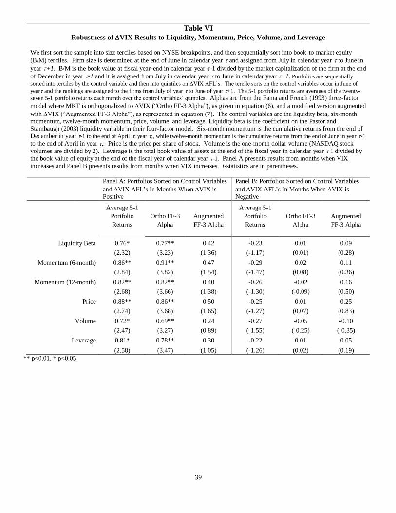
Results for months when VIX increases are in Table VI, Panel A, and findings for
months when VIX decreases are in Table VI, Panel B. When VIX is positive, all 5-1 returns
and three-factor alphas are positive and significant at the 5% level or better, while in the
augmented model all alphas are insignificant. When VIX is negative, all 5-1 returns and alphas
are insignificant. All of these results are very similar to those in Table V and suggest that when
VIX rises there is substantial evidence indicating it is a risk factor, while when VIX falls there is
very little evidence that VIX innovations are a priced risk factor. These results confirm that
liquidity, momentum, price, volume, and leverage are not driving the results from the size and
B/M characteristic-balanced portfolio tests.
Finally, we estimate Fama and MacBeth (1973) cross-sectional regressions with firm-
level data. Consistent with the earlier portfolio analysis, the first monthly cross-sectional
regression is for July, 1989, and independent variables include the AFL on VIX, log of size,
B/M, six-month momentum, beta on MKT⊥, and liquidity beta. The construction of all variables
is as defined earlier. Separate estimations are performed for months when VIX is positive and
for months when it is negative. We employ Newey and West (1987) standard errors in the
construction of t-statistics.
Table VII, Panel A, has results when VIX rises and Panel B has results for when VIX
falls. When VIX rises, the coefficient on VIX loadings is positive and significant at the 5%
level. This is consistent with prior results indicating that when VIX rises, loadings on VIX
matter. When VIX falls, the coefficient on VIX loadings is negative and insignificant. The
absolute value of the coefficient is more than four times higher when VIX rises than when it
24
falls. These results are consistent with prior results and suggest a lesser role for loadings when
VIX is negative.
IV. Results with FVIX
Ang et al. (2006) suggest that using VIX at the monthly level is a poor approximation
for changes in aggregate volatility due to the role that the conditional mean of VIX plays in the
determination of the unanticipated change in VIX, as well as the possibility that jump risk and
the stochastic volatility risk premium may be incorporated in VIX. This inspires them to create a
factor mimicking portfolio, FVIX, that proxies for innovations in aggregate volatility and can be
used at any frequency. In order to ensure that our results are not due to an inappropriate proxy
for innovations in aggregate volatility, we create FVIX as detailed by Ang et al., and perform the
same analysis as in the previous section, replacing VIX with FVIX. All steps in the analysis
are identical, except that FVIX replaces VIX in the models and equations.
Panel A of Table VIII shows the equal- and value-weighted returns, the pre-formation
and post-formation AFL’s, and the size and B/M of the quintile portfolios single-sorted by
AFL’s on FVIX. The FVIX AFL’s are slightly less dispersed than those based on VIX. The
size and B/M characteristics of the quintiles portfolios are similar between the quintile portfolios
based on the FVIX AFL’s and those based on VIX AFL’s. The 5-1 portfolio returns are not
significantly different from zero and similar in magnitude to VIX results in Table II.
In Panels B and C of Table VIII, the equal- and value-weighted returns of the 5-1
portfolios are given conditional on the contemporaneous sign of FVIX. When FVIX is positive,
25
the 5-1 returns and three-factor alphas are positive and significant at the 1% level. Their
magnitudes are about twice the corresponding measures for VIX in Table II. When FVIX is
negative, the 5-1 returns are negative and significant. The three-factor alphas are negative, but
only the value-weighted alpha is significant, and the alphas are about half the 5-1 returns. These
results are different from the VIX results in Table II where there was no significance.15
The story is somewhat different when FVIX is negative than when VIX declines. With
FVIX, a partial risk explanation is warranted because loadings seem to matter. However, two
things should be noted. First, the 5-1 returns and alphas are much smaller when FVIX is
negative than when it is positive; thus, the risk explanation is stronger in the latter than the
former. Second, when FVIX is negative there is still a strong positive effect on returns
irrespective of loadings; the smallest return of the ten portfolios is 2.68%, which is actually
slightly larger than the smaller corresponding returns in Table II for a negative VIX. Our prior
conclusion, that when implied volatility falls there is a substantial positive return effect just for
being a stock and irrespective of loadings, remains; however, risk matters too. The asymmetric
volatility phenomenon remains intact when substituting FVIX for VIX as the proxy for
innovations in aggregate volatility.
As with VIX, we examine the stability of the FVIX AFL’s from the pre-formation
period to the post-formation period. The methodology is the same and results are in Table IX.
The pre-formation AFL’s on FVIX are well dispersed, and the rankings and dispersion generally
hold for post-formation AFL’s. The dispersion is not as great, however, as it was for VIX.
15 FVIX has a greater mean, standard deviation, and range than VIX. This may lead to greater dispersion in returns
with FVIX than VIX.
26
This is the same conclusion as when the VIX loadings in Table II, Panel A, are compared with
the FVIX loadings in Table VI, Panel A.
Panels A and B of Table X present value-weighted returns for the nine size and B/M
sorted portfolios from periods when FVIX is positive and negative, respectively.16
Results are
very similar to those for VIX in Table IV. When FVIX is positive (negative), portfolio returns
and three-factor alphas are negative (positive) and highly significant. Magnitudes of returns and
alphas are slightly greater with FVIX. FVIX strongly affects portfolio returns in a similar way
that VIX does.
We now look at returns for the nine portfolios where each is divided into five portfolios
based on AFL’s. Panel A of Table XI presents results for months when FVIX is positive and
Panel B has results for months when FVIX is negative. When FVIX is positive, all nine 5-1
returns and alphas from the three-factor model with MKT⊥ (the MKT factor orthogonalized to
FVIX), SMB, and HML are positive and significant at the 1% level, except for two alphas that
are significant at 5%. The joint alpha test is significant at the 1% level. The three-factor model
augmented with FVIX has six of nine alphas insignificantly different from zero and the joint
alpha test is insignificant. Typical augmented model alphas keep about one-half the value of the
three-factor alphas, even though only three are significant. These results are very similar to
those with VIX, indicating a strong market volatility risk component and a possible residual
unexplained effect too.
When FVIX is negative, eight of nine 5-1 returns are negative and significant at the 5%
level or better. This is different from results with VIX where all 5-1 returns are insignificant.
16 As with VIX, unreported results with equal-weighted returns for FVIX are similar to value-weighted returns.
27
Two of nine alphas from the three-factor model with MKT⊥, SMB, and HML are significant, one
each at the 1% and 5% levels, respectively. The joint test alpha is insignificant. Thus, much of
the 5-1 return differences are explained by the three-factor model, reducing the chances that the
5-1 differences are due to FVIX loadings. However, the typical three-factor alpha is about 40%
of the typical 5-1 return difference. This, coupled with two significant alphas, suggests that there
may be a minor risk-based explanation for 5-1 return differences. This conclusion is slightly
different than with VIX, where there is no significance and no risk story. Like with VIX,
alphas from the augmented three-factor model with FVIX are insignificant. Finally, all 45
portfolio returns are strongly positive, even more so than they are with VIX. Thus, the message
when FVIX is negative is fairly similar to that when VIX is negative. There are strong positive
returns across all portfolios, suggesting a positive effect on the returns of all stocks, irrespective
of loadings, when FVIX or VIX is negative. When expected market volatility changes are
measured by FVIX, there may be a minor risk aspect to the explanation.
V. Conclusion
We examine the effect of innovations in implied volatility on stock returns and whether
the relation is best described as due to risk or characteristics. Importantly, we address these
relations in the context of asymmetric volatility. We use returns contemporaneous to the
portfolio formation and account for the asymmetric volatility phenomenon by using a model that
allows different loadings for positive and negative innovations in implied market volatility. We
apply a test from Daniel and Titman (1997) to distinguish risk from characteristics. We find that
a firm’s sensitivity to changes in market volatility is a cross-sectionally priced risk factor when

28
volatility increases, but not when it decreases. Loadings matter when volatility rises, but when
volatility falls there is a positive uniform effect on all stock returns.
Monthly loadings of stock returns on VIX are obtained via rolling regressions from
January 1986 through December 2007. Portfolios are constructed based on their past loadings
and then examined to see if there is a difference in returns among them. Sensitivities to VIX
are found to have a cross-sectional effect on returns. Next, stocks are sorted into portfolios with
like size and B/M characteristics, and then sorted into portfolios based on their adjusted factor
loadings on VIX. Inside of each size and B/M bin, a characteristic-balanced zero-cost portfolio
is formed that is long in stocks that load high on VIX and short stocks that load low on VIX.
We examine results separately for months when VIX is positive and for months when it is
negative.
When VIX is positive the zero-cost portfolios have significantly positive returns, alphas
from a three-factor model, including an orthogonalized market factor, that are also positive and
significant, and alphas from a three-factor model augmented with VIX innovations that are
generally positive and insignificant. These results suggest that VIX loadings are a priced risk
factor. There are some minor positive abnormal returns that tend to remain in the augmented
model alphas, however. When VIX is negative, zero-cost returns and all alphas are
insignificant. Further, all characteristically balanced non-zero cost portfolios have strongly
positive returns that are roughly equivalent. These results suggest that when VIX is negative,
risk related to VIX innovations does not matter, with positive returns just for being a stock. Our
results are robust to liquidity, momentum, price, volume, and leverage.
29
We examine results from Fama and MacBeth (1973) firm-level regressions and reach
similar conclusions to our portfolio analysis. We then examine portfolio results based on the
FVIX measure derived by Ang et al. (2006). For increasing volatility, results are similar to those
with VIX. When volatility decreases, a minor risk component appears with FVIX that was not
present with VIX. However, there is an even stronger positive effect on returns, fairly uniform
across portfolios, just for being a stock, than there was with VIX. Overall, the pricing of
volatility risk is more complex than previously thought and warrants further study.
30
References
Adrian, Tobias, and Joshua Rosenberg, 2008, Stock returns and volatility: pricing the short-
run and long-run components of market risk, Journal of Finance 63, 2997-3030.
Ang, Andrew, Robert Hodrick, Yuhang Xing, and Xiaoyan Zhang, 2006, The cross section of
volatility and expected returns, Journal of Finance 51, 259–299.
Bekaert, Geert, and Guojun Wu, 2000, Asymmetric volatility and risk in equity markets,
Review of Financial Studies 13, 1-42.
Bakshi, Gurdip, and Nikunj Kapadia, 2003, Delta-hedged gains and the negative market
volatility risk premium, Review of Financial Studies 16, 527–566.
Campbell, John Y., 1993, Intertemporal asset pricing without consumption data, American
Economic Review 83, 487–512.
Campbell, John Y., 1996, Understanding risk and return, Journal of Political Economy 104,
298–345.
Campbell, John Y., and Ludger Hentschel, 1992, No news is good news: An asymmetric
model of changing volatility in stock returns, Journal of Financial Economics 31, 281–
318.
Chen, Joseph, 2003, Intertemporal CAPM and the cross-section of stock returns, Working
paper, University of Southern California.
Daniel, Kent, and Sheridan Titman, 1997, Evidence on the characteristics of cross-sectional
variation in stock returns, Journal of Finance 52, 1-33.
Daniel, Kent, Sheridan Titman, K. C. John Wei, 2001, Explaining the cross-section of stock
returns in Japan: Factors or Characteristics?, Journal of Finance 56, 743-766 .
Davis, James, Eugene F. Fama, and Kenneth R. French, 2000, Characteristics, covariances,
and average returns: 1929-1997, Journal of Finance 55, 389-406.
Dennis, Patrick, Stewart Mayhew, and Chris Stivers, 2006, Stock returns, implied volatility
innovations, and the asymmetric volatility phenomenon, Journal of Financial and
Quantitative Analysis 41, 381-406.
Fama, Eugene F., and Kenneth R. French, 1992, The cross-section of expected stock returns,
Journal of Finance 47, 427-465.
Fama, Eugene F., and Kenneth R. French, 1993, Common risk factors in the returns on
stocks and bonds, Journal of Financial Economics 33, 3–56.
31
Fama, Eugene F., and James MacBeth, 1973, Risk, return, and equilibrium: empirical tests,
Journal of Political Economy 71, 607-636.
French, Kenneth R., G. William Schwert, and Robert F. Stambaugh, 1987, Expected stock
returns and volatility, Journal of Financial Economics 19, 3–30.
Gibbons, Michael R., Steven A. Ross, and Jay Shanken, 1989, A test of the efficiency of a
given portfolio, Econometrica 57, 1121–1152.
Glosten, Lawrence R., Ravi Jagannathan, and David E. Runkle, 1993, On the relation
between expected value and the volatility of the nominal excess return on stocks, Journal
of Finance 47, 1779–1801.
Heston, Steven L., 1993, A closed-form solution for options with stochastic volatility with
applications to bond and currency options, Review of Financial Studies 6, 327-343.
Jegadeesh, Narasimhan, and Sheridan Titman, 1993, Returns to buying winners and selling
losers: Implications for stock market efficiency, Journal of Finance 48, 65–92.
Lakonishok, Josef, Andrei Shleifer, and Robert W. Vishny, 1994, Contrarian investment,
extrapolation, and risk, Journal of Finance 49, 1541-1578.
Merton, Robert C., 1973, An intertemporal asset pricing model, Econometrica 41, 867–887.
Newey, W., and Kenneth D. West, 1987, A simple, positive semi-definite, heteroskedasticity and
autocorrelation consistent covariance matrix, Econometrica 55, 703-708.
Pastor, Lubos, and Robert F. Stambaugh, 2003, Liquidity risk and expected stock
returns, Journal of Political Economy 111, 642–685.
Whaley, Robert, 2000, The investor fear gauge, Journal of Portfolio Management 26, 12–17.
Wu, Guojun, 2001, The determinants of asymmetric volatility, Review of Financial Studies 14, 837-859.

32
Table I Monthly Factor Correlations
The table reports the correlations between the Fama and French (1993) factors MKT, SMB, and HML, the first
differences in VIX (VIX), and the factor mimicking portfolio FVIX (constructed similar to Ang et al. (2006)).
Panel A reports the correlations over the entire sample period of January 1986 to December 2007. Panel B
reports the correlations during the months when MKT is positive. Panel C reports the correlations during the
sample period when MKT is negative.
Panel A: Monthly Correlations for the Entire Sample Period
MKT SMB HML VIX FVIX
MKT 1.0000
SMB 0.1926 1.0000
HML -0.5013 -0.3152 1.0000
VIX -0.5558 -0.2864 0.1274 1.0000
FVIX -0.5961 -0.1937 0.2358 0.6510 1.0000
Panel B: Monthly Correlations When Excess Market Returns Are Positive
MKT SMB HML VIX FVIX
MKT 1.0000
SMB -0.0060 1.0000
HML -0.4186 -0.4213 1.0000
VIX -0.1808 -0.1364 0.0101 1.0000
FVIX -0.2681 0.0544 0.2952 -0.0287 1.0000
Panel C: Monthly Correlations When Excess Market Returns Are Negative
MKT SMB HML VIX FVIX
MKT 1.0000
SMB 0.2531 1.0000
HML -0.3692 -0.1014 1.0000
VIX -0.6981 -0.3620 0.0175 1.0000
FVIX
-0.7197 -0.2688 0.1095 0.7924 1.0000
33
Panel A: Portfolios sorted by the AFL’s on VIX for the entire sample period.
Post-formation Monthly Returns (%)
Mean of
Pre-
formation
VIX AFL
Mean of
Post-
formation
VIX AFL
VIX AFL Quintiles Equal weighted Value weighted Log of size B/M
1 (Low) 1.38 0.76 -3.21 -2.85 4.68 0.75
2 1.25 0.96 -1.39 -1.32 5.38 0.79
3 1.23 0.92 -0.71 -0.73 5.60 0.76
4 1.28 0.93 -0.11 -0.23 5.46 0.77
5 (High) 1.72 1.24 1.25 0.86 4.65 0.81
5-1 0.34 0.48
(1.44) (1.62) ** p<0.01, * p<0.05
Table II Portfolios Sorted by Sensitivity to Innovations in Implied Market Volatility
For each firm a regression is estimated of the form:
𝑟𝑖 ,𝑡 = 𝛼𝑖 + 𝛽∆𝑉𝐼𝑋 ,𝑖∆𝑉𝐼𝑋𝑡 + 𝜃𝑖𝑃𝑂𝑆𝑡∗∆𝑉𝐼𝑋𝑡 + 𝜀𝑖 ,𝑡
where ri,t is the excess return for firm i in month t, VIXt is the innovation in VIX from the end of month t-1 to the end of month t, POSt is a dummy variable that equals one in months when VIX is positive and equals zero otherwise, and i,t is an error term. This
regression is estimated for each firm for June of year on a monthly basis over 54 months (a minimum of 36 months of data are
required) ending in December of year -1. The beta and theta estimates for each June of year are assigned to July of year
through June of year +1. Although each firm’s parameter estimates are held constant for twelve-month periods, they are used to
create VIX adjusted factor loadings (VIX AFL’s) each month using the realized value of POSt for each respective month from
July of year through June of year +1. The VIX AFL’s are computed as:
𝐴𝐹𝐿∆𝑉𝐼𝑋 ,𝑖 ,𝑡 = 𝛽 ∆𝑉𝐼𝑋 ,𝑖 + 𝜃 𝑖𝑃𝑂𝑆𝑡
Firms are sorted each month into quintiles based on their VIX AFL’s. Post-formation monthly returns are averages of stock returns (either equal- or value-weighted) in each portfolio every month. Post-formation loadings are found by rolling the
regressions every month to obtain monthly parameter estimates for each firm. AFL’s are computed for each firm each month. The
portfolio post-formation AFL’s are averages of the post-formation AFL’s of the firms in the quintile portfolios sorted by the pre-
formation AFL’s. Panel A presents equal- and value-weighted average monthly returns in the post-formation period, the mean
AFL’s for the pre- and post-formation periods, average natural log of mean size (total market capitalization) and the average book-
to-market equity ratio (B/M) of the firms in each quintile portfolio. The row “5-1” refers to the mean difference in returns between
quintile portfolios 5 and 1. Panels B and C report the equal and value-weighted portfolio returns and the mean difference in returns
between quintile portfolios 5 and 1, but limit the sample to months where either the VIX is positive or negative, respectively. The alpha from regressing the 5-1 portfolio returns on the Fama and French (1993) three-factor model, with a market factor
orthogonalized to VIX, is reported in the row labeled “Ortho FF-3 Alpha.” t-statistics are reported in parentheses.
34
Panel B: Portfolios sorted by the AFL’s on VIX when VIX is positive. Panel C: Portfolios sorted by the AFL’s on VIX when VIX is negative.
Post-formation Monthly Returns (%) Post-formation Monthly Returns (%)
VIX AFL Quintiles Equal weighted Value weighted VIX AFL Quintiles Equal weighted Value weighted
1 (Low) -1.04 -1.52 1 (Low) 3.72 2.97
2 -0.68 -0.76 2 3.12 2.62
3 -0.47 -0.56 3 2.87 2.34
4 -0.33 -0.50 4 2.82 2.30
5 (High) -0.07 -0.17 5 (High) 3.45 2.61
5-1 0.97* 1.34** 5-1 -0.27 -0.36
(2.35) (2.90) (-1.26) (-1.03)
Ortho FF-3 Alpha 0.71* 1.21** Ortho FF-3 Alpha -0.01 -0.01
(2.56) (3.42) (-0.05) (-0.02)
** p<0.01, * p<0.05

35
Table III
Stability of VIX Adjusted Factor Loadings
This table reports the pre- and post-formation mean VIX AFL's in each portfolio that is sequentially sorted by size, book-to-market equity ratio (B/M), and VIX AFL’s. We first sort the sample into size terciles based on NYSE breakpoints, and then sequentially sort into book-to-market equity (B/M) terciles. The size of the
firm is determined at the end of June in calendar year and assigned to the firm from July in calendar year to June in year +1. B/M is the book value at fiscal
year-end in calendar year -1 divided by the market capitalization of the firm at the end of December in year -1 and it is assigned to the firm from July in calendar
year to June in +1. In each size and B/M portfolio bin the stocks are divided into equal quintiles based on their pre-formation VIX AFL's formed from
estimated parameters in June of year . Post-formation loadings are obtained by estimating equation (1) for each firm and rolling the regressions every month to obtain monthly parameter estimates. AFL’s are computed for each firm each month using equation (2). The portfolio post-formation AFL’s are averages of post-
formation AFL’s of the firms in the quintile portfolios sorted by the pre-formation AFL’s.
Pre-formation Mean VIX AFL Post-formation Mean VIX AFL
Size B/M VIX AFL Quintiles VIX AFL Quintiles
Rank Rank 1 (Low) 2 3 4 5 (High) Average 1 (Low) 2 3 4 5 (High) Average
1 (Low) 1 (Low) -4.20 -1.84 -0.87 0.01 1.88 -1.00 -3.70 -1.74 -0.92 -0.17 1.32 -1.04
1 2 -3.11 -1.34 -0.65 -0.05 1.22 -0.79 -2.75 -1.27 -0.67 -0.17 0.86 -0.80
1 3 -3.16 -1.39 -0.66 0.00 1.34 -0.77 -2.77 -1.29 -0.66 -0.12 0.97 -0.77
2 1 -3.12 -1.51 -0.85 -0.25 0.94 -0.96 -2.78 -1.45 -0.89 -0.34 0.52 -0.99
2 2 -2.39 -1.24 -0.70 -0.23 0.68 -0.78 -2.16 -1.16 -0.70 -0.31 0.42 -0.78
2 3 -2.26 -1.18 -0.68 -0.25 0.55 -0.76 -2.05 -1.13 -0.72 -0.36 0.30 -0.79
3 1 -2.31 -1.14 -0.66 -0.22 0.64 -0.74 -2.06 -1.12 -0.70 -0.33 0.35 -0.77
3 2 -2.00 -1.08 -0.65 -0.26 0.48 -0.70 -1.83 -1.04 -0.66 -0.33 0.24 -0.72
3 (High) 3 (High) -1.88 -1.03 -0.63 -0.24 0.45 -0.67 -1.71 -0.98 -0.66 -0.35 0.23 -0.69
36
Table IV Mean Returns and Alphas of the Nine Portfolios Formed on the Basis of Size
and Book-to-Market Ratio
We first sort the sample into size terciles based on NYSE breakpoints, and then sequentially sort into book-to-market equity (B/M)
terciles. Firm size is determined at the end of June in calendar year and assigned from July in calendar year to June in year +1.
B/M is the book value at fiscal year-end in calendar year -1 divided by the market capitalization of the firm at the end of December
in year -1 and it is assigned from July in calendar year to June in calendar year +1. Value-weighted returns for each portfolio are calculated every month from July 1989 to December 2007. Panel A contains months where VIX increases and Panel B has
months where it decreases. Alphas are from the Fama and French (1993) three- factor model where MKT is orthogonalized to VIX
(“Ortho FF-3 Alpha”). The row labeled “Joint test p-value” presents the p-value from a Gibbons, Ross, and Shanken (1989) multivariate test of alphas. The last row shows the mean returns and alphas when the characteristic-balanced portfolio returns are
averaged across size and B/M sorted portfolios each month. t-statistics are in parentheses.
Panel A: Mean Returns and Alphas in
Months When VIX is Positive
Panel B: Mean Returns and Alphas in
Months When VIX is Negative
Size B/M Log of
B/M Portfolio Returns Ortho FF-3
Alpha Portfolio Returns Ortho FF-3
Alpha Rank Rank Size
1(Low) 1(Low) 4.32 0.28 -1.84** -2.11** 2.90** 1.58**
(-3.03) (-8.49) (5.54) (5.02)
1 2 4.21 0.70 -0.75 -1.40** 2.64** 1.57**
(-1.69) (-6.84) (7.67) (7.19)
1 3 3.48 1.74 -0.81 -1.51** 2.85** 1.56**
(-1.65) (-6.08) (6.84) (5.55)
2 1 6.79 0.23 -1.59** -2.00** 2.90** 1.76**
(-2.80) (-6.80) (6.08) (6.91)
2 2 6.77 0.48 -0.95* -1.74** 2.49** 1.51**
(-2.12) (-7.50) (7.72) (7.17)
2 3 6.75 0.92 -0.93* -1.86** 2.62** 1.58**
(-2.13) (-7.86) (8.27) (8.32)
3 1 8.94 0.18 -1.03* -1.47** 2.16** 1.54**
(-2.27) (-7.23) (5.74) (6.68)
3 2 8.71 0.40 -0.91* -1.65** 2.24** 1.57**
(-2.32) (-7.07) (7.28) (6.91)
3(High) 3(High) 8.52 0.76 -0.89* -1.91** 2.30** 1.59**
(-2.16) (-8.95) (7.52) (7.14)
Joint test p-value 0.0000 0.0000
Average across portfolios -1.08* -1.74** 2.57** 1.58**
(-2.50) (-8.34) (8.13) (9.06)
** p<0.01, * p<0.05

37
Table V Mean Returns and Alphas of Portfolios Formed on the Basis of Size,
Book-to-Market, and VIX Adjusted Factor Loadings
We first sort the sample into size terciles based on NYSE breakpoints, and then sequentially sort into book-to-market equity (B/M)
terciles. Firm size is determined at the end of June in calendar year and assigned from July in calendar year to June in year +1.
B/M is the book value at fiscal year-end in calendar year -1 divided by the market capitalization of the firm at the end of December
in year -1 and it is assigned from July in calendar year to June in calendar year +1. In each size and B/M portfolio bin the stocks
are divided into equal quintiles each month based on the pre-formation VIX AFL’s. Value-weighted returns are calculated for each portfolio every month from July 1989 to December 2007. Mean returns for each triple-sorted portfolio and the 5-1 characteristic-
balanced portfolios are presented. Alphas are from the Fama and French (1993) three-factor model where MKT is orthogonalized to
VIX (“Ortho FF-3 Alpha”), as given in equation (6), and a modified version augmented with VIX (“Augmented FF-3 Alpha”), as represented in equation (7). The row labeled “Joint test p-value” presents the p-value from a Gibbons, Ross, and Shanken (1989)
multivariate test of alphas. The last row shows the mean returns and alphas when the characteristic-balanced portfolio returns are
averaged across size and B/M sorted portfolios each month. Panels A and B report portfolio returns for months when VIX is positive or negative, respectively. t-statistics are in parentheses.
Panel A: Mean Returns of Portfolios Sorted on Size, B/M, and VIX AFL’s In Months When VIX is Positive
Average Post-formation Monthly Returns (%)
Size Rank B/M Rank
VIX AFL Quintiles
5-1
Ortho FF-3
Alpha
Augmented FF-3
Alpha 1 (Low) 2 3 4 5 (High)
1 (Low) 1 (Low) -2.16 -1.61 -1.11 -1.00 -0.80 1.36** 1.13** 0.45
(3.21) (3.18) (1.00)
1 2 -0.78 -0.22 -0.29 -0.17 -0.02 0.75 0.67 -0.17
(1.59) (1.89) (-0.39)
1 3 -0.44 -0.58 -0.43 -0.33 0.57 1.01** 1.25** 0.83
(2.81) (3.43) (1.75)
2 1 -1.53 -1.13 -1.44 -0.54 -0.57 0.96* 0.90* 0.62
(1.98) (2.25) (1.20)
2 2 -1.03 -0.21 -0.47 -0.56 -0.23 0.80 0.82* 0.42
(1.69) (2.15) (0.85)
2 3 -0.70 -0.48 -0.61 -0.38 -0.14 0.56 0.64* 0.10
(1.50) (2.04) (0.26)
3 1 -1.75 -0.53 -0.64 -0.52 -0.09 1.66** 1.52** 1.52*
(3.19) (3.34) (2.56)
3 2 -0.91 -0.80 -0.68 -0.32 -0.16 0.75 0.71* 0.08
(1.92) (2.08) (0.19)
3 (High) 3 (High) -0.66 -0.49 -0.64 -0.42 0.32 0.98* 1.09** 0.62
(2.03) (2.83) (1.23)
Joint test p-value 0.0031 0.1289
Average across portfolios 0.98** 0.97** 0.50
(2.86) (3.92) (1.58)
** p<0.01, * p<0.05

38
Panel B: Mean Returns of Portfolios Sorted on Size, B/M, and VIX AFL’s In Months When VIX is Negative
Average Post-formation Monthly Returns (%)
Size Rank B/M Rank
VIX AFL Quintiles
5-1
Ortho FF-3
Alpha
Augmented FF-3
Alpha 1 (Low) 2 3 4 5 (High)
1 (Low) 1 (Low) 3.45 3.16 2.62 2.90 3.03 -0.41 -0.38 -0.43
(-1.30) (-1.09) (-0.83)
1 2 3.29 2.96 2.56 2.69 3.20 -0.09 -0.09 0.11
(-0.32) (-0.27) (0.22)
1 3 3.19 2.97 2.90 2.82 3.55 0.36 0.58 0.19
(1.06) (1.60) (0.36)
2 1 3.20 2.80 2.68 2.84 3.09 -0.12 0.16 -0.38
(-0.37) (0.47) (-0.78)
2 2 2.98 2.70 2.59 2.49 2.63 -0.35 -0.10 0.25
(-1.23) (-0.34) (0.57)
2 3 3.01 2.99 2.70 2.80 2.61 -0.40 -0.03 -0.09
(-1.47) (-0.11) (-0.21)
3 1 2.73 2.44 2.44 2.14 2.31 -0.41 0.16 0.36
(-0.98) (0.37) (0.55)
3 2 2.81 2.78 2.16 2.52 2.34 -0.46 0.08 0.66
(1.27) (0.22) (1.17)
3 (High) 3 (High) 2.94 2.87 2.36 2.22 2.51 -0.42 -0.04 -0.17
(-1.30) (-0.10) (-0.34)
Joint test p-value 0.6906 0.6998
Average across portfolios -0.26 0.04 0.05
(-1.20) (0.17) (0.16)
** p<0.01, * p<0.05
39
Table VI
Robustness of VIX Results to Liquidity, Momentum, Price, Volume, and Leverage
We first sort the sample into size terciles based on NYSE breakpoints, and then sequentially sort into book-to-market equity
(B/M) terciles. Firm size is determined at the end of June in calendar year and assigned from July in calendar year to June in
year +1. B/M is the book value at fiscal year-end in calendar year -1 divided by the market capitalization of the firm at the end
of December in year -1 and it is assigned from July in calendar year to June in calendar year +1. Portfolios are sequentially
sorted into terciles by the control variable and then into quintiles on VIX AFL’s. The tercile sorts on the control variables occur in June of
year and the rankings are assigned to the firms from July of year to June of year +1. The 5-1 portfolio returns are averages of the twenty-
seven 5-1 portfolio returns each month over the control variables’ quintiles. Alphas are from the Fama and French (1993) three-factor
model where MKT is orthogonalized to VIX (“Ortho FF-3 Alpha”), as given in equation (6), and a modified version augmented
with VIX (“Augmented FF-3 Alpha”), as represented in equation (7). The control variables are the liquidity beta, six-month momentum, twelve-month momentum, price, volume, and leverage. Liquidity beta is the coefficient on the Pastor and Stambaugh (2003) liquidity variable in their four-factor model. Six-month momentum is the cumulative returns from the end of
December in year -1 to the end of April in year ,, while twelve-month momentum is the cumulative returns from the end of June in year -1
to the end of April in year ,. Price is the price per share of stock. Volume is the one-month dollar volume (NASDAQ stock
volumes are divided by 2). Leverage is the total book value of assets at the end of the fiscal year in calendar year -1 divided by
the book value of equity at the end of the fiscal year of calendar year -1. Panel A presents results from months when VIX
increases and Panel B presents results from months when VIX increases. t-statistics are in parentheses.
Panel A: Portfolios Sorted on Control Variables
and VIX AFL’s In Months When VIX is Positive
Panel B: Portfolios Sorted on Control Variables
and VIX AFL’s In Months When VIX is Negative
Average 5-1
Portfolio
Returns
Ortho FF-3
Alpha
Augmented
FF-3 Alpha
Average 5-1
Portfolio
Returns
Ortho FF-3
Alpha
Augmented
FF-3 Alpha
Liquidity Beta 0.76* 0.77** 0.42 -0.23 0.01 0.09
(2.32) (3.23) (1.36) (-1.17) (0.01) (0.28)
Momentum (6-month) 0.86** 0.91** 0.47 -0.29 0.02 0.11
(2.84) (3.82) (1.54) (-1.47) (0.08) (0.36)
Momentum (12-month) 0.82** 0.82** 0.40 -0.26 -0.02 0.16
(2.68) (3.66) (1.38) (-1.30) (-0.09) (0.50)
Price 0.88** 0.86** 0.50 -0.25 0.01 0.25
(2.74) (3.68) (1.65) (-1.27) (0.07) (0.83)
Volume 0.72* 0.69** 0.24 -0.27 -0.05 -0.10
(2.47) (3.27) (0.89) (-1.55) (-0.25) (-0.35)
Leverage 0.81* 0.78** 0.30 -0.22 0.01 0.05
(2.58) (3.47) (1.05) (-1.26) (0.02) (0.19)
** p<0.01, * p<0.05

40
Table VII
Fama-MacBeth Regressions with VIX AFL’s, Size, B/M, Momentum, Orthogonalized Market Betas, and
Liquidity Betas
This table reports the Fama and MacBeth (1973) estimated premiums associated with the VIX AFL’s, natural log of size, B/M,
6-month momentum, beta on MKT⊥ (where MKT⊥ is the MKT factor orthogonalized to VIX), and the beta on liquidity (the
coefficient on the Pastor and Stambaugh (2003) liquidity variable in their four-factor model). Firm size is determined at the end
of June in calendar year and assigned from July in calendar year to June in year +1. B/M is the book value at fiscal year-end
in calendar year -1 divided by the market capitalization of the firm at the end of December in year -1 and it is assigned from
July in calendar year to June in calendar year +1. Six-month momentum is the cumulative returns from the end of month t-6 to the end of month t-2. The beta on MKT⊥ is estimated by using the regression:
𝑟𝑖 ,𝑡 = 𝑎𝑖 + 𝛽𝑖𝑀𝐾𝑇𝑡⊥ + 𝜀𝑖 ,𝑡
where ri,t is the return of stock i in month t, MKTt⊥
is market factor in month t that is orthogonalized to VIX, and εi,t is an error
term. This regression is estimated for each firm for June of year on a monthly basis over 54 months (a minimum of 36 months
of data are required) ending in December of year -1. The beta estimates for each June of year are assigned to July of year
through June of year +1. The liquidity betas are estimated using the regression:
𝑟𝑖 ,𝑡 = 𝛼𝑖 + 𝛽𝑖𝑀𝐾𝑇𝑡 + 𝑠𝑖𝑆𝑀𝐵𝑡 + ℎ𝑖𝐻𝑀𝐿𝑡 + 𝑙𝑖𝐿𝐼𝑄𝑡 + 𝜀𝑖 ,𝑡
where MKT, SMB, and HML are the Fama-French (1993) factors and LIQ is the Pastor and Stambaugh liquidity factor. The
sample is from July 1989 to December 2007. Panel A reports the results when VIX increases. Panel B reports the results when
VIX decreases. Robust Newey-West (1987) t-statistics are in parentheses.
Panel A: Months When VIX is Positive Panel B: Months When VIX is Negative
VIX AFL 0.25* -0.06
(2.13) (-1.57)
Log of Size -0.16 -0.15
(-1.62) (-1.58)
B/M 0.43* 0.13
(2.60) (0.93)
Momentum (6-month) 0.85** -0.34
(2.86) (-0.73)
MKT⊥ Beta -0.47* 0.73**
(-2.11) (3.98)
Liquidity Beta -0.002* 0.001
(-2.50) (1.39)
** p<0.01, * p<0.05
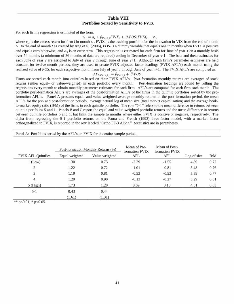
41
Panel A: Portfolios sorted by the AFL’s on FVIX for the entire sample period.
Post-formation Monthly Returns (%) Mean of Pre-
formation FVIX
AFL
Mean of Post-
formation FVIX
AFL
FVIX AFL Quintiles Equal weighted Value weighted Log of size B/M
1 (Low) 1.30 0.75 -2.29 -1.55 4.89 0.72
2 1.22 0.72 -1.01 -0.81 5.48 0.76
3 1.19 0.81 -0.53 -0.53 5.59 0.77
4 1.29 0.90 -0.13 -0.27 5.29 0.81
5 (High) 1.73 1.20 0.69 0.10 4.51 0.83
5-1 0.43 0.44
(1.61) (1.31) ** p<0.01, * p<0.05
Table VIII Portfolios Sorted by Sensitivity to FVIX
For each firm a regression is estimated of the form:
𝑟𝑖 ,𝑡 = 𝛼𝑖 + 𝛽𝐹𝑉𝐼𝑋 ,𝑖𝐹𝑉𝐼𝑋𝑡 + 𝜃𝑖𝑃𝑂𝑆𝑡∗𝐹𝑉𝐼𝑋𝑡 + 𝜀𝑖 ,𝑡
where ri,t is the excess return for firm i in month t, , FVIXt is the tracking portfolio for the innovation in VIX from the end of month
t-1 to the end of month t as created by Ang et al. (2006), POSt is a dummy variable that equals one in months when FVIX is positive
and equals zero otherwise, and i,t is an error term. This regression is estimated for each firm for June of year on a monthly basis
over 54 months (a minimum of 36 months of data are required) ending in December of year -1. The beta and theta estimates for
each June of year are assigned to July of year through June of year +1. Although each firm’s parameter estimates are held constant for twelve-month periods, they are used to create FVIX adjusted factor loadings (FVIX AFL’s) each month using the
realized value of POSt for each respective month from July of year through June of year +1. The FVIX AFL’s are computed as:
𝐴𝐹𝐿𝐹𝑉𝐼𝑋 ,𝑖 ,𝑡 = 𝛽 𝐹𝑉𝐼𝑋 ,𝑖 + 𝜃 𝑖𝑃𝑂𝑆𝑡
Firms are sorted each month into quintiles based on their FVIX AFL’s. Post-formation monthly returns are averages of stock
returns (either equal- or value-weighted) in each portfolio every month. Post-formation loadings are found by rolling the
regressions every month to obtain monthly parameter estimates for each firm. AFL’s are computed for each firm each month. The
portfolio post-formation AFL’s are averages of the post-formation AFL’s of the firms in the quintile portfolios sorted by the pre-
formation AFL’s. Panel A presents equal- and value-weighted average monthly returns in the post-formation period, the mean
AFL’s for the pre- and post-formation periods, average natural log of mean size (total market capitalization) and the average book-
to-market equity ratio (B/M) of the firms in each quintile portfolio. The row “5-1” refers to the mean difference in returns between
quintile portfolios 5 and 1. Panels B and C report the equal and value-weighted portfolio returns and the mean difference in returns
between quintile portfolios 5 and 1, but limit the sample to months where either FVIX is positive or negative, respectively. The alpha from regressing the 5-1 portfolio returns on the Fama and French (1993) three-factor model, with a market factor
orthoganalized to FVIX, is reported in the row labeled “Ortho FF-3 Alpha.” t-statistics are in parentheses.
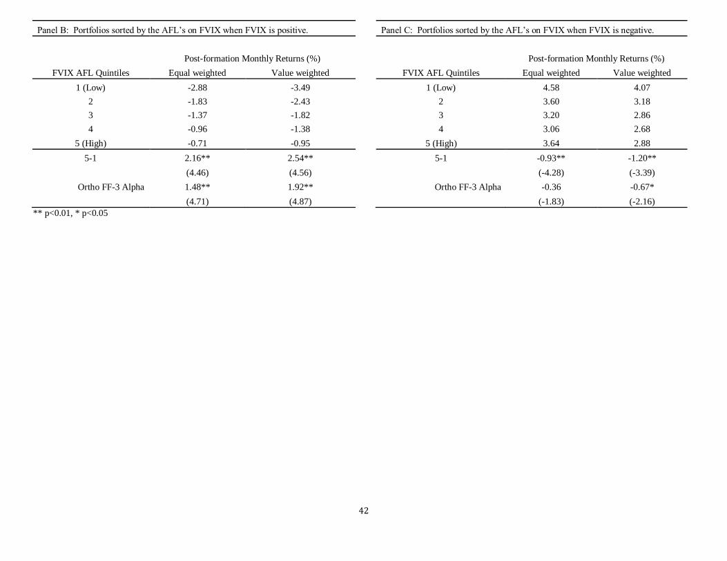
42
Panel B: Portfolios sorted by the AFL’s on FVIX when FVIX is positive. Panel C: Portfolios sorted by the AFL’s on FVIX when FVIX is negative.
Post-formation Monthly Returns (%) Post-formation Monthly Returns (%)
FVIX AFL Quintiles Equal weighted Value weighted FVIX AFL Quintiles Equal weighted Value weighted
1 (Low) -2.88 -3.49 1 (Low) 4.58 4.07
2 -1.83 -2.43 2 3.60 3.18
3 -1.37 -1.82 3 3.20 2.86
4 -0.96 -1.38 4 3.06 2.68
5 (High) -0.71 -0.95 5 (High) 3.64 2.88
5-1 2.16** 2.54** 5-1 -0.93** -1.20**
(4.46) (4.56) (-4.28) (-3.39)
Ortho FF-3 Alpha 1.48** 1.92** Ortho FF-3 Alpha -0.36 -0.67*
(4.71) (4.87) (-1.83) (-2.16)
** p<0.01, * p<0.05
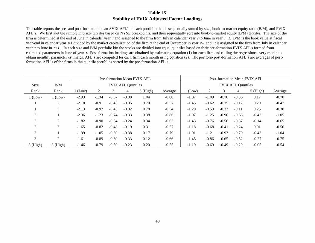
43
Table IX
Stability of FVIX Adjusted Factor Loadings
This table reports the pre- and post-formation mean VIX AFL's in each portfolio that is sequentially sorted by size, book-to-market equity ratio (B/M), and FVIX AFL’s. We first sort the sample into size terciles based on NYSE breakpoints, and then sequentially sort into book-to-market equity (B/M) terciles. The size of the
firm is determined at the end of June in calendar year and assigned to the firm from July in calendar year to June in year +1. B/M is the book value at fiscal
year-end in calendar year -1 divided by the market capitalization of the firm at the end of December in year -1 and it is assigned to the firm from July in calendar
year to June in +1. In each size and B/M portfolio bin the stocks are divided into equal quintiles based on their pre-formation FVIX AFL's formed from
estimated parameters in June of year . Post-formation loadings are obtained by estimating equation (1) for each firm and rolling the regressions every month to obtain monthly parameter estimates. AFL’s are computed for each firm each month using equation (2). The portfolio post-formation AFL’s are averages of post-
formation AFL’s of the firms in the quintile portfolios sorted by the pre-formation AFL’s.
Pre-formation Mean FVIX AFL Post-formation Mean FVIX AFL
Size B/M FVIX AFL Quintiles FVIX AFL Quintiles
Rank Rank 1 (Low) 2 3 4 5 (High) Average 1 (Low) 2 3 4 5 (High) Average
1 (Low) 1 (Low) -2.93 -1.34 -0.67 -0.08 1.04 -0.80 -1.87 -1.09 -0.76 -0.36 0.17 -0.78
1 2 -2.18 -0.91 -0.43 -0.05 0.70 -0.57 -1.45 -0.62 -0.35 -0.12 0.20 -0.47
1 3 -2.13 -0.92 -0.43 -0.02 0.78 -0.54 -1.20 -0.53 -0.33 -0.11 0.25 -0.38
2 1 -2.36 -1.23 -0.74 -0.33 0.38 -0.86 -1.97 -1.25 -0.90 -0.68 -0.43 -1.05
2 2 -1.82 -0.90 -0.54 -0.24 0.34 -0.63 -1.43 -0.76 -0.56 -0.37 -0.14 -0.65
2 3 -1.65 -0.82 -0.48 -0.19 0.31 -0.57 -1.18 -0.68 -0.41 -0.24 0.01 -0.50
3 1 -1.99 -1.05 -0.69 -0.38 0.17 -0.79 -1.91 -1.21 -0.93 -0.70 -0.43 -1.04
3 2 -1.61 -0.89 -0.60 -0.33 0.12 -0.66 -1.45 -0.86 -0.65 -0.52 -0.27 -0.75
3 (High) 3 (High) -1.46 -0.79 -0.50 -0.23 0.20 -0.55 -1.19 -0.69 -0.49 -0.29 -0.05 -0.54
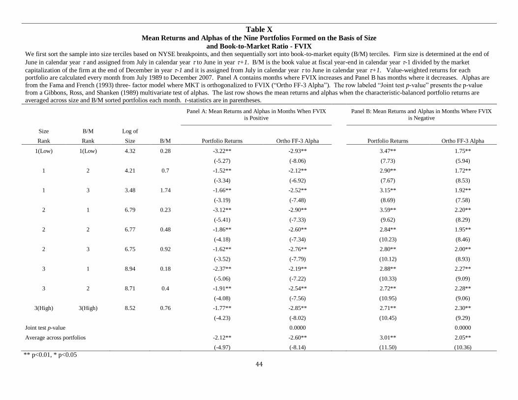
44
Table X Mean Returns and Alphas of the Nine Portfolios Formed on the Basis of Size
and Book-to-Market Ratio - FVIX We first sort the sample into size terciles based on NYSE breakpoints, and then sequentially sort into book-to-market equity (B/M) terciles. Firm size is determined at the end of
June in calendar year and assigned from July in calendar year to June in year +1. B/M is the book value at fiscal year-end in calendar year -1 divided by the market
capitalization of the firm at the end of December in year -1 and it is assigned from July in calendar year to June in calendar year +1. Value-weighted returns for each portfolio are calculated every month from July 1989 to December 2007. Panel A contains months where FVIX increases and Panel B has months where it decreases. Alphas are
from the Fama and French (1993) three- factor model where MKT is orthogonalized to FVIX (“Ortho FF-3 Alpha”). The row labeled “Joint test p-value” presents the p-value
from a Gibbons, Ross, and Shanken (1989) multivariate test of alphas. The last row shows the mean returns and alphas when the characteristic-balanced portfolio returns are
averaged across size and B/M sorted portfolios each month. t-statistics are in parentheses.
Panel A: Mean Returns and Alphas in Months When FVIX is Positive
Panel B: Mean Returns and Alphas in Months Where FVIX is Negative
Size B/M Log of
B/M Portfolio Returns Ortho FF-3 Alpha Portfolio Returns Ortho FF-3 Alpha Rank Rank Size
1(Low) 1(Low) 4.32 0.28 -3.22** -2.93** 3.47** 1.75**
(-5.27) (-8.06) (7.73) (5.94)
1 2 4.21 0.7 -1.52** -2.12** 2.90** 1.72**
(-3.34) (-6.92) (7.67) (8.53)
1 3 3.48 1.74 -1.66** -2.52** 3.15** 1.92**
(-3.19) (-7.48) (8.69) (7.58)
2 1 6.79 0.23 -3.12** -2.90** 3.59** 2.20**
(-5.41) (-7.33) (9.62) (8.29)
2 2 6.77 0.48 -1.86** -2.60** 2.84** 1.95**
(-4.18) (-7.34) (10.23) (8.46)
2 3 6.75 0.92 -1.62** -2.76** 2.80** 2.00**
(-3.52) (-7.79) (10.12) (8.93)
3 1 8.94 0.18 -2.37** -2.19** 2.88** 2.27**
(-5.06) (-7.22) (10.33) (9.09)
3 2 8.71 0.4 -1.91** -2.54** 2.72** 2.28**
(-4.08) (-7.56) (10.95) (9.06)
3(High) 3(High) 8.52 0.76 -1.77** -2.85** 2.71** 2.30**
(-4.23) (-8.02) (10.45) (9.29)
Joint test p-value 0.0000 0.0000
Average across portfolios -2.12** -2.60** 3.01** 2.05**
(-4.97) (-8.14) (11.50) (10.36)
** p<0.01, * p<0.05

45
Table XI Mean Returns and Alphas of Portfolios Formed on the Basis of Size,
Book-to-Market, and FVIX Adjusted Factor Loadings
We first sort the sample into size terciles based on NYSE breakpoints, and then sequentially sort into book-to-market equity (B/M)
terciles. Firm size is determined at the end of June in calendar year and assigned from July in calendar year to June in year +1.
B/M is the book value at fiscal year-end in calendar year -1 divided by the market capitalization of the firm at the end of December in
year -1 and it is assigned from July in calendar year to June in calendar year +1. In each size and B/M portfolio bin the stocks are divided into equal quintiles each month based on the pre-formation FVIX AFL’s. Value-weighted returns are calculated for each
portfolio every month from July 1989 to December 2007. Mean returns for each triple-sorted portfolio and the 5-1 characteristic-
balanced portfolios are presented. Alphas are from the Fama and French (1993) three-factor model where MKT is orthogonalized to
FVIX (“Ortho FF-3 Alpha”) and a modified version augmented with FVIX (“Augmented FF-3 Alpha”). The row labeled “Joint test
p-value” presents the p-value from a Gibbons, Ross, and Shanken (1989) multivariate test of alphas. The last row shows the mean
returns and alphas when the characteristic-balanced portfolio returns are averaged across size and B/M sorted portfolios each month. Panels A and B report portfolio returns for months when FVIX is positive or negative, respectively. t-statistics are in parentheses.
Panel A: Mean Returns of Portfolios Sorted on Size, B/M, and FVIX AFL’s In Months When FVIX is Positive
Average Post-formation Monthly Returns (%)
Size
Rank
B/M
Rank
FVIX AFL Quintiles
5-1
Ortho FF-3
Alpha
Augmented FF-3
Alpha 1 (Low) 2 3 4 5 (High)
1 (Low) 1 (Low) -4.01 -2.92 -2.68 -1.65 -2.33 1.68** 0.90* 0.15
(2.93) (2.16) (0.28)
1 2 -2.30 -1.14 -0.93 -0.84 -0.44 1.86** 1.23** 0.17
(2.73) (2.78) (0.31)
1 3 -1.98 -1.34 -1.10 -0.84 -0.73 2.94** 0.90* 0.29
(4.61) (2.56) (0.64)
2 1 -4.26 -2.82 -2.66 -2.05 -1.31 1.82** 1.70** 1.47*
(3.58) (3.77) (2.46)
2 2 -2.65 -1.65 -1.28 -0.87 -0.83 1.87** 1.68** 1.15*
(4.28) (4.17) (2.18)
2 3 -2.27 -1.18 -1.50 -0.74 -0.40 1.87** 1.78** 0.61
(4.28) (4.87) (1.37)
3 1 -3.76 -2.83 -2.12 -1.26 -1.22 2.54** 1.60** 1.30*
(4.05) (3.44) (2.11)
3 2 -2.78 -1.95 -1.45 -0.97 -0.97 1.81** 1.64** 0.81
(3.79) (3.66) (1.39)
3 (High) 3 (High) -2.02 -1.78 -1.39 -0.96 -0.06 1.96** 1.80** 0.44
(3.66) (3.70) (0.72)
Joint test p-value 0.0005 0.2327
Average across portfolios 1.97** 1.47** 0.71*
(4.39) (5.16) (1.98)
** p<0.01, * p<0.05
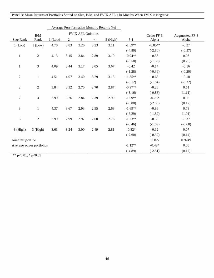
46
Panel B: Mean Returns of Portfolios Sorted on Size, B/M, and FVIX AFL’s In Months When FVIX is Negative
Average Post-formation Monthly Returns (%)
Size Rank
B/M
Rank
FVIX AFL Quintiles
5-1
Ortho FF-3
Alpha
Augmented FF-3
Alpha 1 (Low) 2 3 4 5 (High)
1 (Low) 1 (Low) 4.70 3.83 3.26 3.23 3.11 -1.59** -0.85** -0.27
(-4.80) (-2.80) (-0.57)
1 2 4.13 3.15 2.84 2.89 3.19 -0.94** -0.38 0.08
(-3.58) (-1.56) (0.20)
1 3 4.09 3.44 3.17 3.05 3.67 -0.42 -0.14 -0.16
(-1.28) (-0.39) (-0.29)
2 1 4.51 4.07 3.40 3.29 3.15 -1.35** -0.68 -0.18
(-3.12) (-1.84) (-0.32)
2 2 3.84 3.32 2.70 2.70 2.87 -0.97** -0.26 0.51
(-3.16) (-0.88) (1.11)
2 3 3.99 3.26 2.84 2.39 2.90 -1.09** -0.75* 0.08
(-3.88) (-2.53) (0.17)
3 1 4.37 3.67 2.93 2.55 2.68 -1.69** -0.86 0.73
(-3.29) (-1.82) (1.01)
3 2 3.99 2.99 2.97 2.60 2.76 -1.23** -0.38 -0.37
(-3.46) (-1.09) (-0.68)
3 (High) 3 (High) 3.63 3.24 3.00 2.49 2.81 -0.82* -0.12 0.07
(-2.60) (-0.37) (0.14)
Joint test p-value 0.0827 0.9249
Average across portfolios -1.12** -0.49* 0.05
(-4.89) (-2.51) (0.17)
** p<0.01, * p<0.05
Top Related