


Languages
Pages
Legal

k../i?' .
_ .f
INVESTIGATION OF TURBULENT FLOW IN
HIGHLY CURVED DUCTS WITH APPLICATION
TO TURBOMACHINERY COMPONENTS
i
fi
Z
L
Final Report for Research Contract NAG 3-624
Principal Investigator J.A.C. Humphrey
Research Assistant M.P. Arnal
Department of Mechanical Engineering
University of California, Berkeley
N
(NASA-CR-1J6,)6O) I_.IV_T3TIr,ATIPN jE TUP_ULC'IT
FL:JW IN IiTGHLY CLJRvr_) JUCT3 _ITH APOLTCATTjN
TO TUR_II4ACqlNr_RY CQMD3N_NI _ _inal Renor£
(Cal iforni_-i Univ.) 1,5o p CqCI 200r, 3134

NUMERICAL CALCULATION OF TURBULENT FLOWIN PASSAGE THROUGH A 90 ° BEND
OF SQUARE CROSS SECTION
M.P. Arnal and J.A.C. Humphrey
Department of Mechanical Engineering
University of California, Berkeley
ABSTRACT
Numerical predictions have been performed using a semi-elliptic calculation procedure
for the case of turbulent flow in passage through a 90 ° bend of square cross section. Two
versions of the isotropic turbulent viscosity two equation k-e model were used. One
(WFM) employs the logarithmic law-of-the-waU relation and the notion of equilibrium flow
to set all the necessary boundary conditions at the first grid point adjacent to a solid wall.
The other (VDM) employs Prandtl's original mixing length formulation, in conjunction with
Van Driest's semi-empirical relation for the mixing length, to calculate the turbulent viscos-
ity in the near wall regions of the flow. In this case, boundary conditions for k and e,
required to calculate these quantities in the core of the flow, are obtained by matching the
mixing length and Reynolds number model formulations in an overlapping region of the
flow near the walls. In both cases the results obtained show an improvement over earlier
calculations using an elliptic numerical procedure. This is attributed to the finer grids pos-
sible in the present work. Of the two models, the VDM formulation shows better overall
conformity with the mean flow measurements. Neither model reproduces well the details of
the stress distribution as a result of the implied isotropic turbulent viscosity.
Table of Contents
ACKNOWLEDGEMENTS ......................................................................................... I
LIST OF FIGURES .................................................................................................... 2
NOMENCLATURE .................................................................................................... 9
1. INTRODUCTION ...................................................................................................... 13
1.1. The Problem Considered .................................................................................... 13
1.2. Previous Work .................................................................................................... 14
1.3. Objectives of the Work ...................................................................................... 15
1.4. Outline ................................................................................................................ 16
2. MEAN FLOW EQUATIONS AND THE TURBULENCE MODEL ......................... 17
2.1. Introduction ........................................................................................................ 17
2.2. Governing equations and the problem of closure .............................................. 17
2.3. The Turbulence Model ....................................................................................... 1920
2.4. Boundary Conditions ..........................................................................................
2.5. Summary of the Equations ................................................................................. 26
3. THE NUMERICAL PROCEDURE ........................................................................... 31
3.1. Introduction ........................................................................................................ 31
3.2. Semi-elliptic flows ............................................................................................. 31
3.3. Finite Differencing Procedures ........................................................................... 33
3.3.1. Treatment of Boundary Conditions ......................................................... 35
3.4. The Solution Algorithm ..................................................................................... 38
4. TEST CASES AND DISCUSSION ........................................................................... 44
4.1. Introduction ........................................................................................................ 4444
4.2. Laminar flows .....................................................................................................
4.3. Turbulent flows .................................................................................................. 4653
4.4. Conclusions ........................................................................................................
5. RESULTS AND DISCUSSION ................................................................................. 55
5.1. Introduction ........................................................................................................ 5557
5.2. Results ................................................................................................................66
5.3. Discussion ..........................................................................................................
6. CONCLUSIONS ........................................................................................................ 69
Appendix A: The QUICK scheme formulation ......................................................... 7070
A.1 The problem of interest ......................................................................................70
A.2 Formulation ........................................................................................................70
A.2.1 Grid arrangement ......................................................................................

-- ii
A.2.2 Finite difference approximation of the convective term(s) .......................
A.2.3 Quadratic upstream interpolation ..............................................................
A.2.4 Implementation of QUICK scheme in variable density flows ..................
A.2.5 Treatment of boundary nodes ....................................................................
References ..................................................................................................................
Figures ........................................................................................................................
71
71
74
77
78
81

ACKNOWLEDGEMENTS
This study was funded by NASA Lewis through two Research Grant Awards (NAG
3-624 and NAG 3-735). The authors are grateful to this agency for their support. Special
thanks go to Dr. Peter Sockol of NASA Lewis who took a special interest in the work. The
study has proceeded in close collaboration with Professor B.E. Lauder and his group at the
University of Manchester, Institute of Science and Technology. In particular, we are grate-
ful to Dr. H. Iacovides (UMIST) and Dr. W.M. To (UCB) for their technical support, espe-
cially during the initiation of the investigation.
-2-
LIST OF FIGURES
Figure 1.1.
Figure 1.2.
Figure 2.1.
Figure 2.2.
Figure 2.3.
Figure 3.1.
Figure 3.2.
Figure 3.3.
Figure 4.1.
Figure 4.2.
Figure 4.3.
Figure 4.4.
Figure 4.5.
Figure 4.6.
Flow pattern of the secondary motion in a curved duct of square cross-
section, ri and ro are the inner- and outer- curved wall radii, respectively.
Schematic of test section from Humphrey et al. [1981] showing dimensions,
coordinate system and velocity components of the flow. R ° = (r-ri)/(ro-ri)
is the non-dimensional radial position in the bend.
Coordinate system for boundary condition definitions. The boundary is either
a wall or symmetry plane.
Duct geometry, showing coordinate system and velocity components.
(a) Straight duct. (b) Curved duct.
Illustration of the mixing length region, interface and core flow region in the
VDM formulation.
Main grid node control volume.
Velocity node control volume.
Control volume for intergration of the general 0-variable transport equation.
Centerline velocity for developing laminar flow in a 2D straight channel,
Re=300. Comparison with Schlichting [1979] boundary layer predictions and
McDonald et al. [1972] fully elliptic predictions.
Velocity profiles for developing laminar flow in a 2D straight channel,
Re=300. (a) Comparison with Schlichting [1979] boundary layer predictions.
(b) Comparison with McDonald et al. [1972] fully elliptic predictions.
Centerline velocity for developing laminar flow in a square duct, Re=200.
Comparison with data of Goldstein and Kreid [1967].
Velocity profiles for developing laminar flow in a square duct, Re=200.Comparison with data of Goldstein and Kreid [1967].
Variation of streamwise friction coefficient c/, with number of nodes in across-stream direction. Straight duct laminar flow.
Mean velocity profile for fully developed turbulent channel flow, Re=110,000.
Comparison of predictions using VDM with Laufer [1950] data.
-3-
Figure4.7.
Figure4.8.
Figure4.9.
Figure4.10.
Figure4.11.
Figure 4.12.
Figure 4.13.
Figure 4.14.
Figure 4.15.
Figure 4.16.
Figure 4.17.
Turbulent kinetic energy profile for fully developed turbulent channel flow,Re=ll0,000. Comparison of predictions using VDM with Laufer [1950] data.
Turbulent shear stress profile for fully developed turbulent channel flow,
Re=ll0,000. Comparison of predictions using VDM with Laufer [1950] data.
Mean velocity profile for fully developed turbulent channel flow, Re=110,000.
Comparison of predictions using WFM (standard constants) with Laufer[1950] data.
Turbulent kinetic energy profile for fully developed turbulent channel flow,
Re=If0,000. Comparison of predictions using WFM (standard constants)with Laufer [1950] data.
Turbulent shear stress profile for fully developed turbulent channel flow,
Re=ll0,000. Comparison of predictions using WFM (standard constants)with Laufer [1950] data.
Turbulent shear stress profile for fully developed turbulent channel flow,
Re=ll0,000. Comparison of predictions using WFM (Laufer's constants)with Laufer [1950] data.
Mean velocity profile for fully developed turbulent channel flow, Re=110,000.
Comparison of predictions using WFM (standard constants) and VDM with
interface region at y+ = 10.
Turbulent kinetic energy profile for fully developed turbulent channel flow,
Re=ll0,000. Comparison of predictions using WFM (standard constants) and
VDM with interface region at y÷ = 10.
Energy dissipation profile for fully developed turbulent channel flow,Re=110,000. Comparison of predictions using WFM (standard constants) and
VDM with interface region at y÷ = 10.
Eddy diffusivity 0ae) profile for fully developed turbulent channel flow,
Re=ll0,000. Comparison of predictions using WFM (standard constants) and
VDM with interface region at y+ = 10.
Mean velocity profile for fully developed turbulent channel flow, Re=110,000.
Comparison of predictions using WFM (standard constants) and VDM with
interface region at y+ -- 25.
Figure4.18.
Figure 4.19.
Turbulent kinetic energy profile for fully developed turbulent channel flow,Re=110,000. Comparison of predictions using W'FM (standard constants) and
VDM with interface region at y+ --- 25.
Energy dissipation profile for fully developed turbulent channel flow,
Re=110,000. Comparison of predictions using WFM (standard constants) and
VDM with interface region at y+ = 25.
Figure 4.20.
Figure 4.21.
Eddy diffusivity (/ae) profile for fully developed turbulent channel flow,
Re--110,000. Comparison of predictions using WFM (standard constants) and
VDM with interface region at y+ --- 25.
Centerline velocity for developing turbulent duct flow, Re--.40,000. Com-
parison of predictions using WFM in the near wall region with Melling[1975] data.
Figure 4.22. Centerlme velocity for developing turbulent duct flow, Re=40,000. Com-
parison of predictions using VDM in the near wall region with Melling[1975] data.
Figure 4.23.
Figure 4.24.
Centerline turbulence intensity for developing turbulent duct flow, Re=40,000.
Comparison of predictions using WFM in the near wall region with Melling[1975] data.
Cenlerline turbulence intensity for developing turbulent duct flow, Re=40,000.
Comparison of predictions using VDM in the near wall region with Melling[1975] data.
Figure 4.25.
Figure 4.26.
Contours of Ux/U,.; for fully developed turbulent duct flow, Re=40,000.
Comparison of predictions using VDM (lower left) and W'FM (upper right)with data of Mellmg [1975].
Cross-stream profiles of U;,/Ub for fully developed turbulent duct flow,
Re=40,000. (a) z/Dn = 0.5. (b) :./Dh = 0.25. Comparison of predictions
with data of Meiling [1975].
Figure 4.27. Contours of _/Uct for fully developed turbulent duct flow, Re--40,000. Com-
parison of predictions using VDM (lower left) and WFM (upper right) withdata of Melling [ 1975].
Figure 4.28. Cross-stream profiles of "_/Ucl×lO 2 for fully developed turbulent duct flow,
Re=40,000. (a) z/Dh = 0.5. (b) z/Dh = 0.25. Comparison of predictionswith data of Melling [1975].
Figure 5.1.
Figure 5.2.
Figure 5.3.
Figure 5.4.
Figure 5.5.
Figure 5.6.
Figure 5.7.
Figure 5.8.
Figure 5.9.
Figure 5.10.
Figure 5. I I.
Grid arrangement for curved duct calculations.
Contours of UolUt, for turbulent bend flow, x/D h =-2.5. Comparison ofpredictions using VDM with data of Humphrey [1977].
Contours of Uo/Ub for turbulent bend flow, x/D, =-2. _ Comparison ofpredictions using WFM with data of Humphrey [1977].
Radial profiles of Uo/Ub for turbulent bend flow, x/D, =-2.5.
(a) z/D h = 0.5. (b) z/D, = 0.25. Comparison of predictions with data ofHumphrey [1977].
Contours of _/Ub×lO 2 for turbulent bend flow, x/D/, = -2.5. Comparison ofpredictions using VDM with data of Humphrey [1977].
Contours of _/Ubxl02 for turbulent bend flow, x/D h = -2.5. Comparison ofpredictions using WFM with data of Humphrey [1977].
Radial profiles of _'/UbxlO 2 for turbulent bend flow, X/Dh =-2.5.
(a) z/O h = 0.5. (b) z/D h --0.25. Comparison of predictions with data ofHumphrey [1977].
Contours of turbulent dissipation, ev/U_,xlO 6 for turbulent bend flow,
x/Dh = -2.5. Comparison of predictions using (a) WFM and (b) VDM.
Contours of Uo/Ub for turbulent bend flow, 0 = 0 °. Comparison of predic-tions using VDM with data of Humphrey [1977].
Contours of Uo/Ub for turbulent bend flow, O = 0 °. Comparison of predic-tions using WFM with data of Humphrey [1977].
Radial profiles of Uo/U b for turbulent bend flow, O = 0 °.
(a) z/D h = 0.5. (b) z/O h = 0.25. Comparison of predictions with data ofHumphrey [1977].
Figure 5.12.
Figure 5.13.
Contours of "ff/UbXlO 2 for turbulent bend flow, 0 = 00. Comparison of pred-ictions using VDM with data of Humphrey [1977].
Contours of _/Ubxl02 for turbulent bend flow, 0 = 0 °. Comparison of pred-ictions using WFM with data of Humphrey [1977].

Figure 5.14.
Figure 5.15.
Figure 5.16.
Figure 5.17.
Figure 5.18.
Figure 5.19.
Figure 5.20.
Figure 5.21.
Figure 5.22.
Figure 5.23.
Radial profiles of _/Ubx102 for turbulent bend flow, 0 = 0 °.
(a) z/O h = 0.5. (b) 7./Dh = 0.25. Comparison of predictions with data of
Humphrey [1977].
Cross-stream velocity vector plot for turbulent bend flow, 0 = 0 °. Comparis-
on of predictions using (a) VDM and (b) WFM.
Contours of turbulent dissipation, ev/U_×lO 6 for turbulent bend flow, 0 = 0 °.
Comparison of predictions using (a) WFM and (b) VDM.
Contours of Uo/U b for turbulent bend flow, 0 = 45 °. Comparison of predic-tions using VDM with data of Humphrey [1977].
Contours of Uo/Ub for turbulent bend flow, 0 = 45 °. Comparison of predic-tions using WFM with data of Humphrey [1977].
Radial profiles of Uo/Ub for turbulent bend flow, 0 = 45°.
(a) z/Dh = 0.5. (b) z/Dh = 0.25. Comparison of predictions with data of
Humphrey [1977] and predictions of Humphrey et al. [1981].
Contours of "_IUbx102 for turbulent bend flow, 0 = 45 °. Comparison of
predictions using VDM with data of Humphrey [1977].
Contours of "_/Ub×lO 2 for turbulent bend flow, O = 45 °. Comparison of
predictions using WFM with data of Humphrey [1977].
Radial profiles of _/Ubx102 for turbulent bend flow, 0 = 450.
(a) z/D h = 0.5. (b) z/D h = 0.25. Comparison of predictions with data ofHumphrey [ 1977].
Cross-stream velocity vector plot for turbulent bend flow, 0 = 45 °. Com-parison of predictions using (a) VDM and (b) WFM.
Figure 5.24.
Figure 5.25.
Figure 5.26.
Contours of turbulent dissipation, ev/U_xlO 6 for turbulent bend flow,
0 = 45 °. Comparison of predictions using (a) WFM and (b) VDM.
Contours of Uo/Ub for turbulent bend flow, 0 = 71° Comparison of predic-
tions using VDM with data of Humphrey [1977].
Contours of Uo/Ub for turbulent bend flow, O = 71 ° Comparison of predic-
tions using WFM with data of Humphrey [1977].

-7-
Figure 5.27. Radial profiles of Uo/Ub for turbulent bend flow, 0 = 71 °
(a) z/Dh = 0.5. (b) z/Dh = 0.25. Comparison of predictions with data of
Humphrey [1977].
Figure 5.28. Contours of "_/Ub×lO 2 for turbulent bend flow, 0 = 71 ° Comparison of
predictions using VDM with data of Humphrey [1977].
Figure 5.29.
Figure 5.30.
Figure 5.31.
Contours of "_/UbxlO 2 for turbulent bend flow, 0 = 71 °. Comparison of
predictions using WFM with data of Humphrey [1977].
Radial profiles of "_lUbx102 for turbulent bend flow, 0 = 71°.
(a) z/D h = 0.5. (b) z/Dh = 0.25. Comparison of predictions with data of
Humphrey [1977].
Cross-stream velocity vector plot for turbulent bend flow, 0 = 71 °. Com-
parison of predictions using (a) VDM and (b) WFM.
Figure 5.32.
Figure 5.33.
Figure 5.34.
Figure 5.35.
Figure 5.36.
Figure 5.37.
Figure 5.38.
Figure 5.39.
Contours of turbulent dissipation, ev/U4xlO 6 for turbulent bend flow,
0 = 71 °. Comparison of predictions using (a) WFM and (b) VDM.
Contours of Uo/Ub for turbulent bend flow, 0 = 90 °. Comparison of predic-
tions using VDM with data of Humphrey [1977].
Contours of Uo/Ub for turbulent bend flow, 0 = 90 °. Comparison of predic-
tions using WFM with data of Humphrey [1977].
Radial profiles of Uo/Ub for turbulent bend flow, 0 = 90 °. (a) z/D h = 0.5.
(b) z/D h = 0.25. Comparison of predictions with data of Humphrey [1977]
and predictions of Humphrey et al. [1981].
Contours of "_/UbxlO 2 for turbulent bend flow, 0 = 90 °. Comparison of
predictions using VDM with data of Humphrey [1977].
Contours of _/Ubx102 for turbulent bend flow, O = 90 °. Comparison of
predictions using WFM with data of Humphrey [1977].
Radial profiles of _/Ubxl02 for turbulent bend flow, O = 90°.
(a) z/D h = 0.5. (b) z/Dh = 0.25. Comparison of predictions with data of
Humphrey [1977].
Cross-stream velocity vector plot for turbulent bend flow, 0 = 90 °. Com-
parison of predictions using (a) VDM and (b) WFM.

Figure5.40.
Figure5.41.
Figure5.42.
Contoursof turbulent dissipation, ev/U_xlO 6 for turbulent bend flow,
O = 90 °. Comparison of predictions using (a) WFM and (b) VDM.
Wall pressure coefficient on the symmetry plane of a 90 ° curved duct,Re=40,000. Comparison of calculations using Van Driest model in the nearwall region with wall function model.
Friction coefficient on the symmetry plane of a 90 ° curved duct, Re=40,000.
Comparison of calculations using Van Driest model in the near wall regionwith wall function model.
Figure A. 1.
Figure A.2.
Figure A.3.
Figure A.4.
Control volume for the property node.
Control volume for the velocity node.
Boundary node for a scalar or velocity component parallel to the boundary.
Boundary node for a velocity component perpendicular to the boundary.
NOMENCLATURE
a
A
A +
c/
cp
Cj
c,1
cc:
d
dU
Dj
Dh
De
E
k
lc
/,.
P
Pt
p"
J
P
P
coefficient in finite difference equation 3.3
area, perpendicular to the velocity in the difference equations 3.6, 3.7
non-dimensional empirical constant in equation 2.20
_lr,J(IApU_), friction coefficient
-Ap/(V2pU_), pressure coefficient
= 0.09, proportionality constant in the definition of turbulent diffusivity
j = e, w, n, s, u, d; convection coefficients in discretized equation 3.2
constant in ,,-transport equation 2.29
constant in e-transport equation 2.29
half channel height in two-dimensional channel flow
- A/a, velocity coefficient in velocity correction equation 3.7
j = e, w, n, s; diffusion coefficients in discretized equation 3.2
hydraulic diameter
- (Dh/2Rc)_.Re, Dean number
roughness parameter in the turbulent law of the wall equation 2.12
time-averaged kinetic energy of turbulence
characteristic length in defining/a t
effective distance from the wall in the Van Driest model exponent.
comer regions in duct flows, equation 4.3
mixing length
pressure
-p+(2/3)pk, turbulent pressure term
pressure correction term, in equation 3.5
guessed, best estimate pressure, equation 3.5
velocity strain rate term in definition of vt, equation 2.21
Used in

-10-
Pk
r, O, z
ri
ro
Rc
R"
Re
Rec
Sp
Su
U
Uc
U
U,
U +
x,y,z
y+
Greek
O_
F
Ar
AU
AV
production of kinetic energy
cylindrical coordinates for curved ducts
inner radius of curvature in a curved duct
outer radius of curvature in a curved duct
mean radius of curvature in a curved duct
-(r-ri)/(ro-ri), non-dimensional radial position in a curved duct
• ,pUbDh//a, duct Reynolds number
-pU Ax//a, cell Reynolds number
coefficient of the linear term in the source, S¢
constant coefficient in the source, S,
source term in 0-transport equation, equation 3.1
fluctuating velocity
characteristic velocity in defining the turbulent diffusivity,/a t
-(u-_) _, root mean square of the fluctuating velocity, u
mean velocity
mean velocity at the duct centerline
z(lrJp) _, wall friction velocity
= UI U,, non-dimensional velocity
Cartesian coordinate system for straight ducts and channels
-yU,/v, non-dimensional distance from a wall
under-relaxation factor in equation 3.10
diffusion coefficient in O-transport equation 3.10
finite difference approximation to dr
finite difference approximation to dU
finite difference approximation to dV
-11-
Ax
Ay
Az
AO
E
0
la
lae
Id num
lal
V
Vt
P
crk
or,
Tres
Tw
Subscripts
b
d
e
E
finite difference approximation to dx
finite difference approximation to dy
finite difference approximation to dz
finite difference approximation to dO
time-averaged dissipation of kinetic energy of turbulence
tangential direction in cylindrical coordinates
Von Karman constant in turbulent law-of-the-wall, equation 2.12
dynamic viscosity
-/z+/a t, effective diffusivity
numerical diffusion
turbulent diffusivity
-la/p, kinematic viscosity
=tat/p, kinematic turbulent diffusivity
angle between velocity vector and coordinate direction, equation 5.2
density
turbulent Prandtl/Schmidt number for k
turbulent Prandtl/Schmidt number for e
resultant wall shear stress in duct flows
wall shear stress
generalized scalar variable in transport equation 3.1
angle between resultant shear stress and coordinate direction, equation 2.18
bulk
downstream boundary of P-cell
east boundary of P-cell
east node

-12-
i
n
N
O
P
r
s
S
U
W
W
X
Y
Z
0
interface
north boundary of P-ceil
north node
wall value
P-node
radial direction
south boundary of P-cell
south node
upstream boundary of P-cell
west boundary of P-cell
west node
streamwise direction (Cartesian coordinates)
cross-stream direction
second cross-stream direction
streamwise direction (cylindrical coordinates)
Superscripts
n new
o old
- time-averaged
vector
_ -13-
1. INTRODUCTION
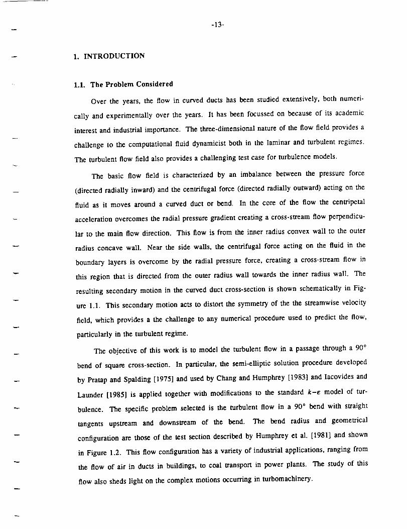
1.1. The Problem Considered
Over the years, the flow in curved ducts has been studied extensively, both numeri-
cally and experimentally over the years. It has been focussed on because of its academic
interest and industrial importance. The three-dimensional nature of the flow field provides a
challenge to the computational fluid dynamicist both in the laminar and turbulent regimes.
The turbulent flow field also provides a challenging test case for turbulence models.
The basic flow field is characterized by an imbalance between the pressure force
(directed radially inward) and the centrifugal force (directed radially outward) acting on the
fluid as it moves around a curved duct or bend. In the core of the flow the centripetal
acceleration overcomes the radial pressure gradient creating a cross-stream flow perpendicu-
lar to the main flow direction. This flow is from the inner radius convex wall to the outer
radius concave wall. Near the side walls, the centrifugal force acting on the fluid in the
boundary layers is overcome by the radial pressure force, creating a cross-stream flow in
this region that is directed from the outer radius wall towards the inner radius wall. The
resulting secondary motion in the curved duct cross-section is shown schematically in Fig-
ure 1.1. This secondary motion acts to distort the symmetry of the the streamwise velocity
field, which provides a the challenge to any numerical procedure used to predict the flow,
particularly in the turbulent regime.
The objective of this work is to model the turbulent flow in a passage through a 90 °
bend of square cross-section. In particular, the semi-elliptic solution procedure developed
by Pratap and Spalding [1975] and used by Chang and Humphrey [1983] and Iacovides and
Launder [1985] is applied together with modifications to the standard k-e model of tur-
bulence. The specific problem selected is the turbulent flow in a 90 ° bend with straight
tangents upstream and downstream of the bend. The bend radius and geometrical
configuration are those of the test section described by Humphrey et al. [1981] and shown
in Figure 1.2. This flow configuration has a variety of industrial applications, ranging from
the flow of air in ducts in buildings, to coal transport in power plants. The study of this
flow also sheds light on the complex motions occurring in turbomachinery.
-- -14-
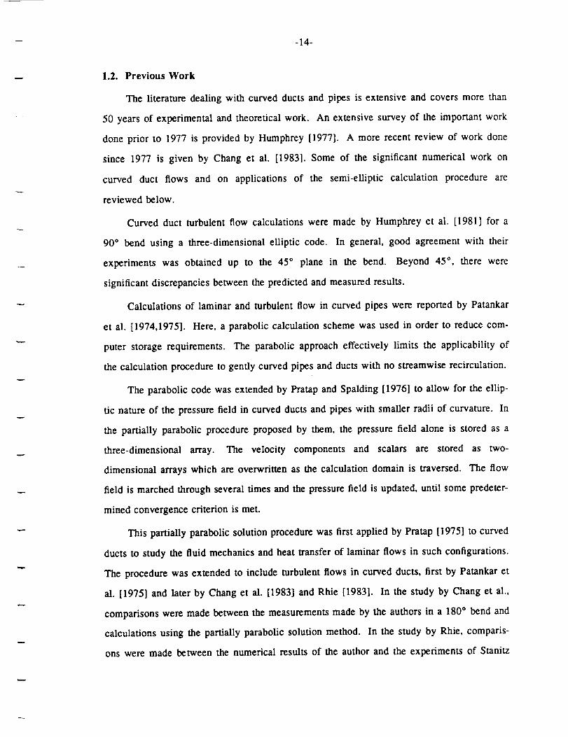
1.2. Previous Work
The literature dealing with curved ducts and pipes is extensive and covers more than
50 years of experimental and theoretical work. An extensive survey of the important work
done prior to 1977 is provided by Humphrey [1977]. A more recent review of work done
since 1977 is given by Chang et al. [1983]. Some of the significant numerical work on
curved duct flows and on applications of the semi-elliptic calculation procedure are
reviewed below.
Curved duct turbulent flow calculations were made by Humphrey et al. [1981] for a
90 ° bend using a three-dimensional elliptic code. In general, good agreement with their
experiments was obtained up to the 45 ° plane in the bend. Beyond 45 ° , there were
significant discrepancies between the predicted and measured results.
Calculations of laminar and turbulent flow in curved pipes were reported by Patankar
et al. [1974,1975]. Here, a parabolic calculation scheme was used in order to reduce com-
puter storage requirements. The parabolic approach effectively limits the applicability of
the calculation procedure to gently curved pipes and ducts with no streamwise recirculation.
The parabolic code was extended by Pratap and Spalding [1976] to allow for the ellip-
tic nature of the pressure field in curved ducts and pipes with smaller radii of curvature. In
the partially parabolic procedure proposed by them, the pressure field alone is stored as a
three-dimensional array. The velocity components and scalars are stored as two-
dimensional arrays which are overwritten as the calculation domain is traversed. The flow
field is marched through several times and the pressure field is updated, until some predeter-
mined convergence criterion is met.
This partially parabolic solution procedure was first applied by Pratap [1975] to curved
ducts to study the fluid mechanics and heat transfer of laminar flows in such configurations.
The procedure was extended to include turbulent flows in curved ducts, first by Patankar et
al. [1975] and later by Chang et al. [1983] and Rhie [1983]. In the study by Chang et al.,
comparisons were made between the measurements made by the authors in a 180" bend and
calculations using the partially parabolic solution method. In the study by Rhie, comparis-
ons were made between the numerical results of the author and the experiments of Stanitz
-15-
et al. [1953] for the caseof subsoniccompressibleflow in an acceleratingrectangular
elbow. In bothcasestheagreementbetweenmeasurementsandpredictionswasbestin the
first 45° of thebend. After the45° plane,theagreementwasqualitativeat best.For the
turbulent calculationsthe boundaryconditionswere imposedusing the wall function
approach,whichminimizesthenumberof grid pointsneededin thenearwall region.
In additionto the applicationsto curvedducts,thepartiallyparabolicor semi-elliptic
procedurehasalsobeenappliedto flowsin curvedpipes,to a turbulentjet in across-stream
(Bergeleset al. [1978])andto otherthree-dimensionalduct flows. For theflows in curved
pipesin particular,a greatdealof work relevantto the presenteffort hasbeendoneby
Iacovides[1986]. The author used a higher order differencingscheme (QUICK) and
applied several techniques designed to stabilize and speed the convergence of the calcula-
tion procedure. Many of these techniques have been incorporated in the present code for
predicting turbulent flows in curved ducts.
From this review of theoretical curved duct studies it becomes apparent that there is a
place for further work in this area. The lack of quantitative agreement between experiments
and calculations beyond the 45 ° plane, and the use of wall functions in the near wall region
which introduce inaccuracies, are areas which need further attention.
1.3. Objectives of the Work
There are two primary objectives which the current study addresses:
1) to evaluate the semi-elliptic calculation procedure as a way of predicting the complex
turbulent flows which occur in curved ducts with small radii of curvature, and
2) to achieve better agreement between predictions of such flows and the experimental
data.
To this end the treatment of the near wall region was evaluated and an alternative to the
wall function approach was studied. Several techniques designed to improve the conver-
gence rates and improve the accuracy of the final results were also evaluated.
-16-
1.4. Outline
The next four sections describe the present study in detail. In section 2 the equations
solved by the calculation procedure are summarized and distinctive features of the specific
turbulence model used are described. To this end, some space is devoted to developing the
treatment for the near wall region which is incorporated into the boundary conditions. Sec-
tion 3 is devoted to a discussion of the numerical procedure used to calculate turbulent
curved duct flows. A brief description of the semi-elliptic calculation technique is given,
followed by a detailed account of the finite differencing scheme and the specific implemen-
tation of the boundary conditions. Finally, the solution algorithm is reviewed.
Both the semi-elliptic numerical procedure and the turbulence model were examined
and compared with experimental or analytical data when possible. The results of the test-
ing, summarized in section 4, demonstrate what can and cannot be expected from the pred-
ictions. They show the limitations of the calculation scheme, and enable one to properly
interpret the results of the final calculations.
In section 5 the results of the calculations of the 90 ° bend are presented. Two sets of
calculations are provided and compared with the experimental data of Humphrey [1977]. In
one set of calculations the standard wall function approach is used in the near wall region.
In the second set of calculations a Van Driest low Reynolds number model is used to treat
the wall region.
Lastly, in section 6 some conclusions are drawn and specific recommendations are
made for future numerical work in this area.
-17-
2. MEAN FLOW EQUATIONS AND THE TURBULENCE MODEL
2.1. Introduction
This section summarizes the mean flow equations governing the flow in curved ducts.
The problem of closure for the set of equations is discussed. The standard k-e model is
briefly described before the derivation of the near wall treatment. Both the wall function
approach and the Van Driesl model for wall bounded flows are presented. The final equa-
tions which are solved, including all the modeled terms, are given at the close of the sec-
lion.
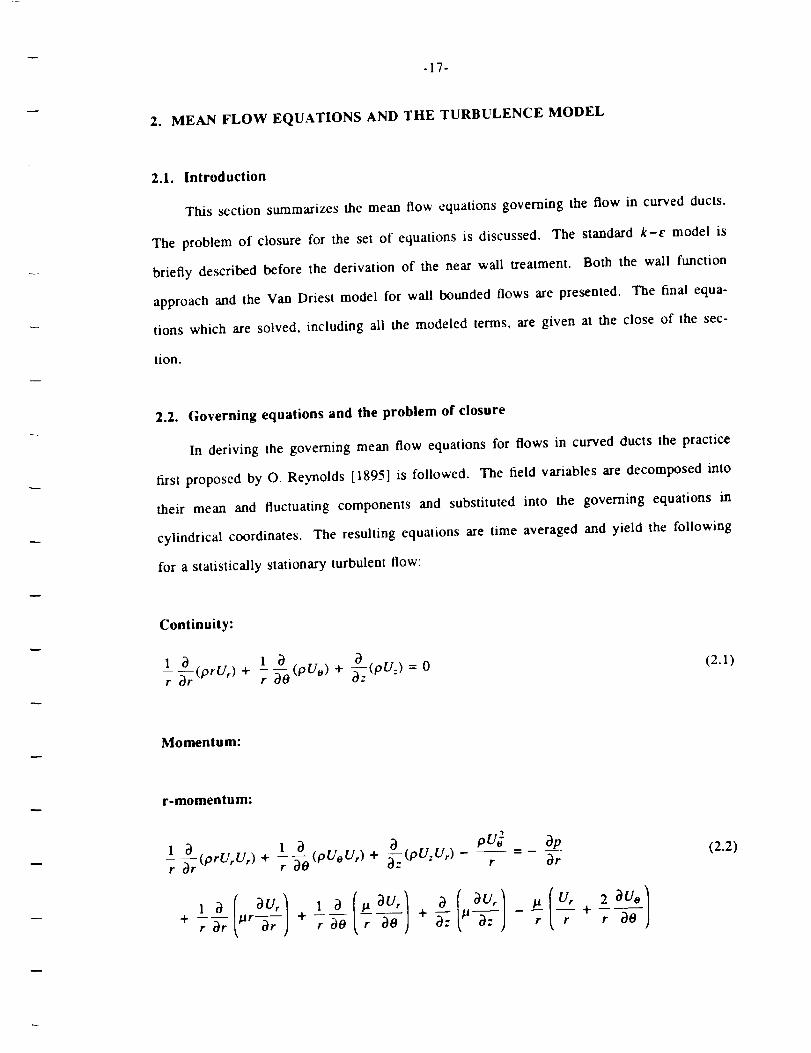
2.2. Governing equations and the problem of closure
In deriving the governing mean flow equations for flows in curved ducts the practice
first proposed by O. Reynolds [1895] is followed. The field variables are decomposed into
their mean and fluctuating components and substituted into the governing equations in
cylindrical coordinates. The resulting equations are time averaged and yield the following
for a statistically stationary turbulent flow:
Continuity:
prUr) + -- pUo) + pU.) = 0r r .
(2.1)
Momentum:
r-momentum:
1 _-r(prUrUr) + I_'o(pUoUr) + _-_(pUzUr) - ----r
= - -- (2.2)r Or
1 _ f 3Ur I 1 _ l__ 3Ur I 3 ( _______rr) _1
U, 2 3Us
r r 30
-18-
I
( 1 ( ++_ ! 3 -P P---P_-r_ + 1 _ -pr +- +
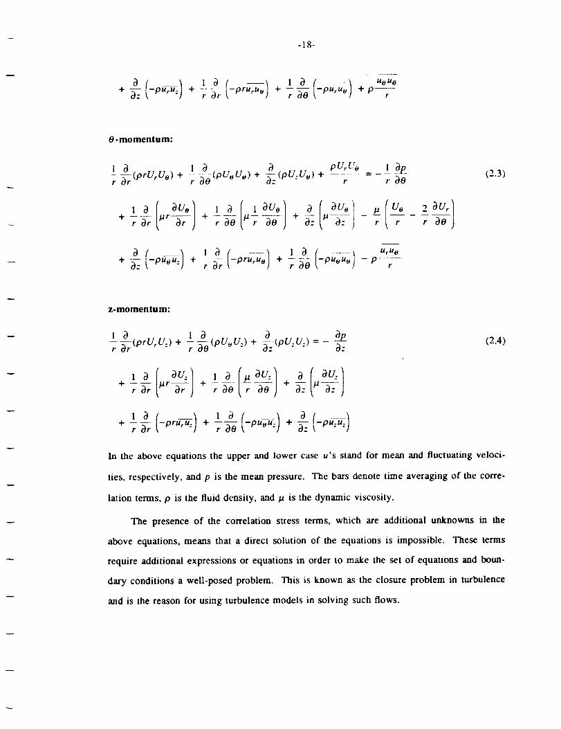
O-momentum:
1 _ (prUrUo)+ 1 __o(PUoUo ) + ff_(pU.Uo )__
r _r r 2 "
P Ur Lr_:_ 1 3pJ¢. ...... _ ---- ....
r r _0
+- -_0)+ ....r_O /Jr _: /J rVe 2aU_ 1
r r o_OJ
( ) '+ (-,:":':-i"r+-pu-_: + 1 _ -pr + ....+ _ r _-r r _-0 -P- r
(2.3)
z-momentum:
l _ (prUrU.) + l__o (pUeU.) + __(pU.U.) = 3pr ar " r " : " " ¢):
•J¢. --rTr r T:
(2.4)
In the above equations the upper and lower case u's stand for mean and fluctuating veloci-
ties, respectively, and p is the mean pressure. The bars denote time averaging of the corre-
lation terms, p is the fluid density, and # is the dynamic viscosity.
The presence of the correlation stress terms, which are additional unknowns in the
above equations, means that a direct solution of the equalions is impossible. These terms
require additional expressions or equations in order to make the set of equations and boun-
dary conditions a well-posed problem. This is known as the closure problem in turbulence
and is the reason for using turbulence models in solving such flows.
-19-
2.3. The Turbulence Model
The turbulence model used in the present work is essentially the high Reynolds
number version of the k-e model, see Rodi [1980], with some modificatioh_ to incorporate
boundary conditions. The closure problem is treated via a Boussinesq assumption, which
defines an isotropic turbulent diffusivity, lit, and uses it to relate the turbulent stresses to the
mean rate of strain tensor. In cylindrical coordinates the six unknown turbulent stresses can
be expressed as:
( OVrt 2(2.5)
-puou o = lit2 OUo U_ ]
---- J - -_pk (2.6)r O0 +2-7- 2
-pu.,,.= u, [- 0z ) -(2.7)
-pUrU o = kit 1 bU, OUo Uo Ir 00 -+ Or r (2.8)
--pUrU z = _It ( _- +
(2.9)
-pueu: = lat
1 OU: OU o ]
r- 0--O- + _J (2.10)
These relations are similar to the constitutive relations for the stress tensor of an incompres-
2sible Newtonian fluid. The additional term -:-pk is included in order to assure that the
3
definition of the turbulent kinetic energy remains unchanged for incompressible flow:
1k = =(u_ + uou o + u._..). (2.11)
Z
The closure problem is now reduced to finding an expression for the distribution of the
turbulent viscosity. This is done by relating the turbulent viscosity to a local velocity and
length scale:

v
-20-
tJl _ puclc
where uc and lc are the appropriate velocity and length scales. For turbulent flows away
from wall boundaries, the appropriate velocity scale is k '_, where k is the turbulent kinetic
energy. The length scale used is 1: = k3/2/E, where e is the dissipation of turbulent kinetic
energy.
The distribution of k and e are determined by solving their respective transport equa-
tions with the associated boundary conditions. Both of these equations can be derived but
contain many terms which must be modeled. A complete description of the derivation of
the k and e equations and the modeling of the various terms which appear in them is given
in Launder and Spalding [1974] and Rodi [1980]. The equations themselves with the
modeled terms are given at the end of this section.
2.4. Boundary Conditions
In this section the treatment of the boundary regions is described and various model-
ing assumptions are given. First, the standard wall function approach (hereafter referred to
as WFM) is explained, then the alternative Van Driest low Reynolds number model
(hereafter referred to as VDM) is given.
Wall Functions
Wall functions are introduced to avoid having to resolve regions of very steep gra-
dients of velocity and turbulence quantities which occur near fixed walls. Instead of apply-
ing boundary conditions at the wall, conditions are effectively fixed at a point near the wall
in the flow field. This point is numerical fixed so as to be in the inertial sublayer region (
30 <y+< 200 ). The influence of the wall on the flow is modeled through setting the boun-
dary conditions at this point. In the following, the two-dimensional case is derived with
reference to Figure 2.1. The extension to three dimensions will then be outlined for the
curved duct.
-21-
For the velocity component parallel to the wall, the logarithmic law of the wall is
assumed to be valid in the inertial sublayer region. The velocity is related to the perpendic-
ular distance from the wall according to:
U_ = 1 ln(Ey÷) (2.12)It"
where E = 9.793 and the Von Karman constant _ = 0.4187. In equation 2.12, U + and y+
are the mean velocity and distance from the wall in wall coordinates and are defined as:
U+ = Ux Y+- yU_U_r v
where U_ is the shear velocity, U_ = z,_-__/p.
For the turbulent kinetic energy, local equilibrium is assumed to hold, and so the pro-
duction of turbulent kinetic energy is equal to the dissipation. This is not unreasonable
since the convection and diffusion of the Reynolds stresses can be shown to be small in this
region near the wall. Therefore, it is assumed that
dU,- e (2.13)
-UxUy dy
The Reynolds stress is related to the mean velocity gradient and the turbulent viscosity is
expressed in terms of the velocity and length scales from the k-e model"
dU:, k2
-UxU v.= vt dy v t c, e (2.14)
where cv is the constant of proportionality. Combining equations 2.13 and 2.14 and recal-
ling that the shear stress in the inertial sublayer is approximately equal to the wall shear
stress gives:
v,- y j = --v: = ,;C-(2.15)
After collecting terms and recalling the definition of the shear velocity U,, the boundary
condition for the turbulent kinetic energy k, in terms of U_ and the proportionality constant

w
-22-
G, is obtained:
V_r °
k - (2.16)c_ t'6
For the dissipation e, the equilibrium assumption is made again and the Reynolds
stress is expressed in terms of the wall shear stress:
__ dG _ dG--= ----" = E'
-UxUy dy p dy
The velocity gradient is determined from the log law of the wall as:
U_+ = lln(Ey+) dU_ _ Ut 2 dUx+ _ U, 2 1_: dy v ay* v ry +
Combining the above expressions for e and dUfldy gives the boundary condition for the
dissipation of kinetic energy e in terms of the wall shear velocity, the Von Karman constant
and the fixed perpendicular distance from the wall:
u, 3e - (2.17)
xy
In three-dimensional flows such as those in curved ducts the wall function approach is
very similar. Figure 2.2 illustrates the basic geometry, coordinate system and velocity com-
ponents for straight and curved ducts. The shear velocity, U, is based on the resultant wall
shear stress, Tre $ where,
tres= _w I + "¢7. 2
since in general, the resultant shear stress is no longer aligned with one of the three coordi-
nate directions. In the above equation the subscripts, 1 and 2 refer to the two shear stress
components parallel to the wall surface. For example, referring to Figure 2.2(a), the resul-
tam shear stress on a wall in the x-z plane would be determined by _,_ and twy, the shear
stresses on the wall due to the x- and z-velocity components respectively. The non-
dimensional wall distance and velocity magnitude are defined as before:
-23-
v+ vu, 1. - - = --In(Ey +)v U_ K:
where U, = z_,_/p and U is the velocity vector parallel to the wall.
The velocity must now be separated into components in the coordinate directions to
apply the boundary conditions. Referring to Figure 2.2(a), there are two velocity com-
ponents, Ux and U: parallel to the walls in the x-: plane.
either of these walls are:
Ux 1= --ln(Ey +) cosv
UT Jc
U._ 1 ln(Ey+) sinlg
U_=O
The boundary conditions at
(2.18)
where tg is the angle between the resultant wall shear stress and the streamwise (x) direc-
tion and y+ is the non-dimensional distance from the side wall. Note that the boundary
conditions for the components parallel to the wall are similar to equation 2.12 for the two-
dimensional case. For the curved duct the treatment of the boundary conditions is similar
for the radial and side walls. The conditions for the turbulence quantities k and e are the
same as those given in equations 2.16 and 2.17 with the shear velocity, U, calculated from
the resultant wall shear stress, 1:,,,. The specifics of how equations 2.16, 2.17 and 2.18 are
incorporated into the numerical scheme, and further details about the governing relations for
the wall function approach can be found in Gosman and Ideriah [1976].
The Van Driest Model
In the derivation of the turbulence model following Prandtl [1925], the eddy viscosity
vt was assumed proportional to a local length and velocity scale. For the k-e model these
scales are combined to give the expressions in equation 2.14. Prandd originally proposed a
simpler and less general mixing length model for which the expressions for the length and
velocity scales for boundary layers are:
- -24-
Uc = It,,
C _" IWI
( ay + ax )
where the coordinates and velocities refer to Figure 2.1.
turbulent diffusivity, vt:
(2.19)
These are combined to form the
, _U bvV t = Im" 2 +
For the case of a fully developed turbulent boundary layer flow the mixing length is propor-
tional to the perpendicular distance from the wall:
lm =
where r is the yon Karman constant.
In shear layers and two-dimensional boundary layers the mixing length model actually
performs reasonably well in predicting features of the flow. The problem in applying the
model to more complex flows lies in determining the appropriate distribution of the local
length scale, l,.. Van Driest [1956] modified the form of the mixing length to account for
wall damping effects. Following his arguments and the analogy to Stokes second problem,
,.=+{1iy+expthe following length is obtained:
(2.20)
where A + is an empirical constant determined to be A + = 26 for a two dimensional boun-
dary layer on a flat plate, and pc is the Von Karman constant.
Using the mixing length model in the near wall region makes it possible to account for
the wall's influence on the core flow directly instead of relying on the wall functions. The
wall functions lump all of the wall influence into the boundary conditions which are fixed in
the flow field rather than at the wall as is most appropriate. In the region near the wall the
mixing length model is used to determine the eddy viscosity distribution. In the core of the
flow the standard k-e model is used. In an interface region between the two, the two
i
-25-
models are matched (see Figure 2.3). The determination of this interface region provides
the boundary conditions for the k and e equations. For the velocities, the boundary condi-
tions are set at the wall by assuming that a laminar sublayer exists in this region.
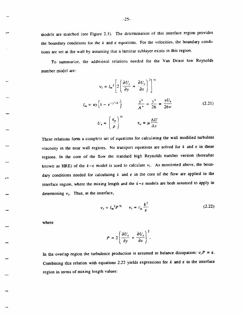
To summarize, the additional relations needed for the Van Driesl low Reynolds
number model are:
V l [ .12]=_,_ 2(_y +_x
I,,,= xy{i - e -y'/A')y+ v + yU,
- -'-- = -- (2.21)A + 26 26v
u, = 3.=*'_7
These relations form a complete set of equations for calculating the wall modified turbulent
viscosity in the near wall regions. No transport equations are solved for k and e in these
regions. In the core of the flow the standard high Reynolds number version (hereafter
known as HRE) of the k-e model is used to calculate v,. As mentioned above, the boun-
dary conditions needed for calculating k and e in the core of the flow are applied in the
interface region, where the mixing length and the k-e models are both assumed to apply in
determining Vr Thus, at the interface,
k 2
vt = l,n2P'_ vt = % e (2.22)
where
_,=2IW + ax J
In the overlap region the turbulence production is assumed to balance dissipation: vrP = e.
Combining this relation with equations 2.22 yields expressions for k and e in the interface
region in terms of mixing length values:

-- -26-
vt 2 lm2p_ (2.23)
k,- , , v2CtaV21m 2 (la
ctaki" I 2p3J2e, - - -m - (2.24)Vt
The subscript i stands for the interfacial values of the quantities in question. These rela-
lions are then used to form boundary conditions for the standard k-e model which is
assumed to hold in the core of the flow. The position of the overlap region is determined
empirically to be y+=10-15.
2.5. Summary of the Equations
In this section the equations which are used to obtain the turbulent flow field in curved
ducts are summarized. The equations contain all the terms and constants as they are
modeled in the numerical scheme. (The constants are taken from Launder and Spalding
[1974].) The boundary conditions which result from the two methods of modeling the near
wall region are also summarized.
Continuity:
r _r (prU') + --r (PUo) + _z-z(PU:)= 0 (2.25)
Momentum:
r-momentum:
l _r(prUrUr) +r 1_-_ (pUeUr) + _'_---(pU'Ur)z"
pug= - -- (2.26)
r Or
,,( "I+ -- /a,r r _ r_O) +r_r 3r) +-- /a,
-27-
r
Ur
r r +_ /al
r 30 /at
13(r_r /a'
Ur
/at r2
r 3r)
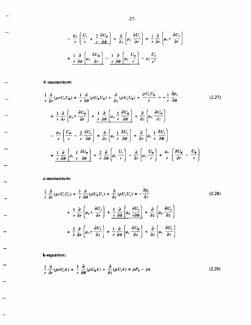
O-momentum:
1 (prUrUs) + _ (pUoUo) + _(pU. Un) +r r -_0 : "pv_v#
+-- r + --
/a, Ue 2 3U_
r r r 3e + - )+-_-z: �at r -_rrr /a' r
r_-O /a' r _0 r_-O �at -_-r �at r
1 3Pt
r 30
uo
r
(2.27)
z-momentum:
1 (prUrU,) + (pUeU_) + (pU.U.) = ---r " Z " " 3Z
+ r_r /aer 3r ) + rffO /ae r301 + _-zz /ae 3z )
+-- + +r_r �air 3z ) r-_ /a' 3. ) _ /at
(2.28)
k-equation:
1 3 (prUrk)+ l _o(pUok)+-_(pU.k)=pP.-per 3r(2.29)

-- -28-
+-- +--r dr _rk crk r _ /_ O'k
e-equation:
1 _ (prUre) + 1 (pUee) + (pU.e) = Col p -_Pk - C¢2P kr 3I" r " "
+-- +--r +-- + -- + IA+--
(2.30)
where
k 2
/J, =/zt +/J Pt = pc_ e c_ = 0.09 Cc_ = 1.44 CE2 = 1.92
2
cq. = 1.0 ac = 1.3 Pt =P + -_pk
([l)/ /2( 12 ( 13u_ " 1 3uo ue 1 3u, 0uoPk = /__Z 2 + ---- + ----
p _ r 30 " r r 00 + -_r-r
..[..1(,,.r+ +---- + ....r r r dO r _O 3r + r 30 Oz
(11(1( 1I ")2( )3Ur 3U: Us 2 3uo " o 1 Ou, :
+ 0: Or + _ + + -- +r _ r 00
r 30
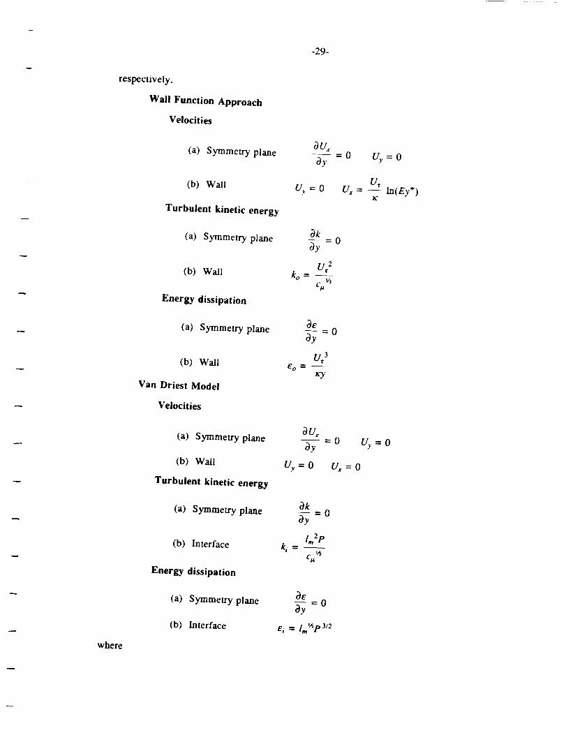
Boundary Conditions
For the purpose of defining the boundary conditions the coordinates and velocities are
shown in Figure 2.1. Note that the definitions are for a x-y coordinate system shown with
U_ and Uy, the velocity components parallel and perpendicular to the boundary,
-29-
respectively.
Wall Function Approach
Velocities
bu,(a) Symmetry plane - 0
by
U_= -- ln(Ey +)(b) Wall Uv, = 0 Us _:
Turbulent kinetic energy
bk--=0
(a) Symmetry plane by
UT2
(b) Wall ko - cu _
Energy dissipation
be--=0
(a) Symmetry plane by
v, 3(b) Wall eo-
ry
Van Driest Model
Velocities
bu_
(a) Symmetry plane by - 0 Uy
Cb) Wall uy = 0 us = o
Turbulent kinetic energy
at--"0
(a) Symmetry plane by
lm2p
(b) Interface ki- ,/iCtt
Energy dissipation
be--=0
(a) Symmetry plane by
(b) Interface ei - I,,"_P 3_2
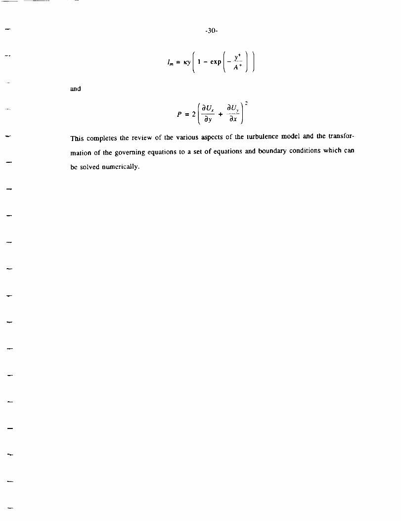
where
U.v=0
=0
-30-
and
Im = ry 1 - exp -A_
e--2 -fir ÷ _xj
This completes the review of the various aspects of the turbulence model and the transfor-
mation of the governing equations to a set of equations and boundary conditions which can
be solved numerically.
-31-
3. THE NUMERICAL PROCEDURE
3.1. Introduction
The results presented in this report were all obtained with a modified three-
dimensional version of the TEACH code developed at Imperial College [1976]. The
modifications in the calculation procedure were made by Chang and Humphrey [1983]
along the lines proposed by Pratap [1975], and take advantage of the semi-elliptic nature of
strongly curved duct flows. The modifications and validation of the numerical procedure
are fully described in Chang and Humphrey [1983]. in the following section a general
description of semi-elliptic flows is presented. In section 3.3 the finite difference procedure
is described and in section 3.4 the solution algorithm is summarized.
3.2. Semi-elliptic flows
Strictly speaking, all subsonic flows are elliptic in nature. Physically, this means that
a change of conditions at any point in the flow field can influence the conditions at any
other point. The information can be transmitted from one point to the other by molecular
diffusion, convection or pressure waves in the fluid. In order to obtain a mathematical solu-
tion to such a problem, boundary conditions for all the dependent variables must be
specified on all boundaries of the flow field. From a computational point of view such
problems are often time consuming and expensive to solve. Fortunately, simplifying
approximations to the equations and boundary conditions can often be made for the problem
of interest. These give rise to two further classes of fluid flow problems, the parabolic flow
and the semi-elliptic (partially-parabolic) flow.
In a parabolic flow one assumes that convection is the only means of transport in the
main flow direction. Such problems do not require boundary conditions for the flow vari-
ables on the downstream boundary. Computationally, such flows can be solved using
marching techniques with a large saving of computer storage and time. At any time in the
solution procedure, values for the dependent variables are needed only at the previously cal-
culated step in order to calculate the unknowns at the next downstream location. For
three-dimensional problems the dependent variables are stored in two-dimensional arrays
-32-
rather than m the three-dimensionalarraysrequired in the counterpart elliptic problem.
Examples of such flows include boundary layers, thin shear layers, steady pipe flows and
mildly curved duct flows.
The semi-elliptic or partially-parabolic flows, as one might expect, are flows which
have some characteristics of both elliptic and parabolic flows. Transport in the main flow
direction is assumed to be by convection only, with molecular diffusion being neglected.
However, changes in the downstream flow can influence the upstream flow behavior through
the pressure field which is treated elliptically. The solulion procedure for semi-elliptic
problems is similar to that for parabolic problems. Boundary conditions for the dependent
variables are not required in the downstream direction and such problems can also be solved
using marching techniques.
The distinction between the two types of problems lies in the treatment of the pressure
field. In a parabolic problem the pressure is treated like any other dependent variable,
determined at any point by its value at the immediate upstream plane. In a semi-elliptic
problem the pressure is treated as an elliptic variable field. This means that the pressure at
any one location is dependent on the value at every other location in the flow field. So, for
a three-dimensional semi-elliptic problem, the pressure must be stored as a three-
dimensional array while all the other variables can be stored as two-dimensional arrays.
Also, time-marching through the flow field once only is no longer sut_cient to determine
the values of the flow field variables, since the downstream locations would have no effect
on the upstream values. Instead, the solution is determined iteratively by marching through
the field several times and updating the pressure field at each iteration.
The semi-elliptic treatment essentially extends the range of flow problems which can
be solved using cost effective marching techniques. Among the flow geometries which can
be effectively handled are strongly curved duct flows (with no streamwise recirculation) and
jet flows in a cross-stream.

-33-
3.3. Finite Differencing Procedures
As a result of treating the flow field in curved ducts as a semi-elliptic problem, the
terms which are underlined in the governing equations given in chapter 2 can be neglected.
Each of the equations can then be written in the same general form given below as a tran-
sporl equation for 1he general variable _"
l° l+l+°1+l lr 3r (prUrep) + -- (pU_¢) + (pU:_) - rF _,r -" r _r -_r- + F + S o (3.1)
where F is the diffusion coefficient for #_ and S_ is the source term for ¢, which contains
all the remaining terms.
The discretization of the general transport equation is done as in the TEACH family of
programs, see Gosman and lderiah [1976]. A staggered grid system is set up in which the
main grid nodes are the storage locations for the pressure and other scalar fields such as the
turbulent kinetic energy, k, dissipation, e, density, p, and viscosity, ju (control volume
shown in Figure 3.1). The velocity components are stored at points midway between the
main grid nodes (control volume shown in Figure 3.2). The treatment of the streamwise
velocity is modified in the semi-elliptic procedure. In order to march through the flow field,
it is convenient to locate the streamwise velocity a half-step ahead of the main grid node
rather than behind as is the case in the elliptic version. This grid system enhances the sta-
bility of the solution procedure and minimizes the amount of interpolation necessary in per-
forming the calculations.
To obtain the finite difference form of the general transport equation, equation 3.1 is
integrated over the control volume for $ shown in Figure 3.3. Using central differencing
for the diffusion terms and leaving the convection terms unspecified for the moment, the
discretized form of equation 3.1 becomes:
C,t#, - Cw_w + CnePn - C_t#+ + Ca_pa - C,¢p, = (3.2)
Dc(¢E - Ct,) - Dw(¢Pe - tPw) + Dn(tPN - (PP) - IDs(t_e - ¢_s) + S, AV
where Ce = (r Ar AO ),(pU:)e ; Cw = (r Ar AO )w(PU:)w
-34-
Cn = (rAzAO)_(pUr)n "
Ca = (ArAz)a(pUo) a ;
O_ --
r Ar AO
z_12
D. - r Ar AO || F. ;
Ar j n
A V = r Ar AO Az
C_ = (rAzAO)s(pU,) s
C. = (ArAz).(pUu)=
Dw _ rArAOJAz _, F.
r Ar A8D s - F s
Ar$
S_,--= -AV1_S_r dr dO dz
where all the subscripts refer to Figure 3.3.
As is the practice in TEACH type programs the source term is linearized as
S, = Sv + Sp0p. This practice proves to be beneficial in adding stability to the solution
procedure and is fully described in Patankar [1980]. The accuracy of the solution and sta-
bility of the numerical procedure have proven to be very sensitive to the prescription of the
O's in the convective terms at the control volume interfaces. A summary of the
differencing schemes used in the present study is given next.
For the 0's at the upstream and downstream locations (0,, On), upwind differencing
was always used for the calculations presented in this report. In this scheme the values for
the 0 's are given as Oa = _p and ¢,,, = 0,g where 0,g is the value of 0,* at the neighboring
upstream location, (or, the "old" 0p-value). This differencing method is in keeping with the
assumptions made for mar, "ing through the flow field in semi-elliptic problems.
For the O's at the cross-stream locations (0,, 0s, 0,, 0w ) the hybrid differencing
method was used for the calculations presented. This scheme, which was first proposed by
Spalding [1972], is based on an approximation to the exact solution of the one-dimensional
convection-diffusion equation. Depending on the local control volume Peclet number either
a central-differencing or upwind-downwind differencing approximation is made. Details of
the specific use of the hybrid scheme are given in Chang and Humphrey [1983]. What is
important to note is that the scheme results in a very stable form of the difference equa-
tions. The drawback to the this scheme is that it is only first order accurate in regions

-35-
where convection dominates. This leads to the possibility of serious errors in the solution
due to numerical diffusion which makes the evaluation of turbulence models more difficult.
For these reasons as well as others, the higher order quadratic-upwind scheme
(QUICK) first proposed by Leonard [1979] has come into increasing usage. The details of
this differencing scheme as it is used by our research group are summarized by S. L. Yuan
in Appendix A. While all of the calculations presented in the report were done using the
hybrid differencing scheme, it is proposed to incorporate the QUICK scheme into the pro-
gram in future work. The advantages to be gained from reduced numerical diffusion fax
outweigh the disadvantages of potential stability problems which can result from careless
use of the quadratic differencing.
After the form of the difference scheme is determined, the interface values of ¢ can be
determined in terms of the values of ¢ at the main grid nodes (P,N,S,E,W). The difference
equation 3.2 can then be written in the following form for the general field variable, ¢:
4
apOp = Y_a_¢. + Su (3.3)n=l
where the a,,'s are coefficients of the ¢,'s and are determined by the local convective and
diffusive coefficients of equation 3.2. Details of how the coefficients are determined are
given in Patankar [1980] for the hybrid scheme as well as several others.
3.3.1. Treatment of Boundary Conditions
This section presents the incorporation of the boundary conditions into the numerical
procedure. There are four different types of boundaries which occur in the calculation of
straight and curved ducts: the inlet, wall, symmetry plane and outlet. For each type of
boundary a numerical treatment must be determined for the three velocity components as
well as for the turbulence quantities, k and _. The numerical representation of the boundary
conditions must reproduce faithfully the exact mathematical formulation (as given in section
2.5) in order to obtain as accurate a solution of the flow field as possible.
With reference to Figure 1.2, at the inlet plane of a straight channel or duct, a plug
flow profile is prescribed for both the laminar and turbulent cases. The streamwise velocity
-36-
component is set to the bulk velocity and the cross-stream velocities are set to zero. For
turbulent flow in a straight channel, empirical profiles for the turbulent kinetic energy and
dissipation are given. These profiles are due to Coles and Hirst [1968] and are for turbulent
flow past a flat plate. For the straight duct the profile for the turbulent kinetic energy is set
to 0.045% of the main flow kinetic energy. This corresponds to a turbulence intensity of
approximately 1.2%. The inlet value of k was chosen to be small compared to final fully
developed values which in duct flows. Estimates of the turbulent kinetic energy distribu-
tion in duct flows were determined using experimental values for the wall shear stress and a
semi-empirical equation relating the shear stress coefficient to the duct Reynolds number.
From Kays and Crawford [1980] for 3x10⁴ < Re < 106:
cl-- = 0.023Re -°-22
where
is the shear stress coefficient.
Cf 'r w
This is related to the shear velocity, U, as
't'w0 _- 0.023Re- '-.
For a duct Reynolds number of Re = 40,000, this corresponds to
U_ = 0.0028U_.
In fully developed duct flows, the value of k + (= k/U_) is known to vary between approxi-
mately 1.0 at the centerline and a maximum of 3.5 near the wall (see e.g. Laufer [1954]).
Combining the above relations for the turbulent kinetic energy k, and the shear velocity U,,
gives estimates of the bounds on the expected k-profile:
k0.0028 < -- < 0.0070
vg
-37-
The inlet profile of k was chosen to be less than 20% of the expected centerline value for
fully developed flow so thal incoming turbulence would not significantly affect the flow
development in the duct. The dissipation profile is prescribed by setting
C3/4 __3/"_
E - (3.4)
where I,,,isthe mixing lengthdeterminedfrom a generalizationof Nikuradse'sstraightpipe
formula for square ducts by Chang and Humphrey [1983]. For the inletconditionsto the
curved duct,the fullydeveloped outletprofilesof the velocitycomponents and turbulence
quantitiesfrom the straightduct calculationsare used. The flow in the straightduct calcu-
lationswas assumed tobe fullydeveloped when the profilesof thevelocitiesand turbulence
quantitiesdid not change in the streamwise direction.These calculationsare discussed
furtherin the sectionon testcases. The profilesare computed using eitherwall functions
(WFM) or the Van Driestmodel (VDM) in the near wallregiondepending on which isto
be used in the curvedduct calculations.
At the symmetry plane of the ducl or channel,the velocityperpendicularto the sym-
metry plane issetto zeroas wellas thenormal gradientof theremainingtwo velocitycom-
ponentsand allotherscalarquantities.
AI the wails,the boundary conditionsdepend on which turbulencemodel is used in
the near wall region. When the WFM formulationis used the boundary conditionsare
specifiednear the wall ratherthan at the wall,as outlinedin seclion2.4. The grid point
nearestthe wall isassumed to liein a regionwhere the logarithmiclaw of the wallholds.
It is furtherassumed thatthe turbulenceis in a stateof localequilibrium(productionof
kineticenergy = dissipation,Pk = 6). With theseassumptionsthe boundary conditionsfor
the threevelocitycomponents and the turbulencequantities,k and 6, can be seLas given in
section2.5.
When the VDM formulationisused inthe nearwallregionthe zerovelocityboundary
conditionisappliedatthe wallforthe threevelocitycomponents. The boundary conditions
for k and E are setatthe interfacebetween the regionwhere the Van Driestmodel (VDM)
appliesand thatwhere Lhe high Reynolds number model (HRE) applies.In the interfacial
-38-
region it is assumed that the turbulence is in local equilibrium and that both the Van Driest
and standard k-e models are valid. With these assumptions the conditions for k and e at
the interface given in section 2.5 can be derived.
Finally, the conditions at the outlet plane are those of a fully developed flow. In this
situation the normal gradients of all the dependent variables are set to zero. In all of the
cases examined these conditions yielded satisfactory results and provided few problems with
stability or convergence.
3.4. The Solution Algorithm
The code developed by Chang and Humphrey [1983] has been substantially modified
in order to obtain the results reported here. The semi-elliptic procedure proposed by Pratap
[1975] was used with several modifications suggested by lacovides [1986]. In the semi-
elliptic solution procedure the basic strategy can be summarized as follows. All the depen-
dent variables (Uo, Ur. U. k, e, etc.) with the exception of the pressure axe stored as two-
dimensional arrays and continuously updated. The pressure field alone is stored as a three-
dimensional array covering the entire flow field. The solution domain is swept through
using a plane-by-plane marching technique until a converged solution is obtained. At each
step in the marching procedure the sequence begins with the computation of the three velo-
city components at the current plane. The respective momentum equations are solved using
the upstream station values from the current sweep for the velocities and the current plane
values of the previous sweep for the pressure. A pressure correction equation is then solved
and the current plane velocity field is corrected to satisfy continuity. The current plane
pressure field is also updated through the pressure correction equation. Lastly the transport
equations of the turbulence quantities are solved. The sequence is then repeated at the next
downstream station until the entire flow field has been traversed. This makes up one pass
through the flow field. Generally, several passes are required to obtain a converged solu-
tion.
The procedure of correcting the current plane velocity and pressure fields to satisfy
continuity is part of the SIMPLE algorithm of Patankar and Spalding [19721. The algo-
rithm was introduced with reference to parabolic flows and extended to elliptic flows;
-39-
Patankar [1980]. It is the standard pressure solver used in the TEACH type elliptic codes.
It has also been used with some modifications in the semi-elliptic calculations of Pratap
[1975], Chang et al. [1983] and lacovides [1986]. The algorithm is briefly summarized
here. The dependent variables are assumed to take the form of equations 3.5:
p=p +p
U=U'+U"
(3.5)
where the superscripts (*) and (') refer to the estimated values and the correction terms,
respectively. The procedure begins with a guessed pressure field, p*. Discretized momen-
tum equations are solved to give a "starred" velocity field. For example, the equation for
the velocity at the east boundary of the P-cell would be:
4
a,U_ = _,a,_U_ + Su + (P_ - p_)A, (3.6)n=l
where the subscripts in equation 3.6 refer to Figure 3.2, A, is the perpendicular control
volume area and the rest of the terms are the same as before. Note also, that equation 3.6
is in the form of equation 3.3. The resulting velocity field satisfies the momentum equa-
tions subject to the guessed pressure field, p'. A pressure correction equation derived from
the continuity equation (see Patankar [1980], for details) is then solved to give a pressure
correction field, p'. The "starred" pressure and velocity fields are then corrected to satisfy
continuity. The velocity and pressure corrections are related as follows:
U,' = Ae (p e' - PE') = dUe.(pp' - p_.') (3.7)ae
where the subscripts refer again to Figure 3.2. This simplified relation between the pressure
and velocity corrections is approximate and only true as the two corrections approach zero.
The resulting corrected velocity field will, in general no longer satisfy the momentum equa-
tions. A number of iterations are therefore necessary to obtain a velocity field which
satisfies both the momentum and continuity equations.
The algorithm is uncomplicated and has been applied to a wide variety of problems
with success. Nevertheless the use of the simplified pressure-velocity correction relation
-4O-
decreasesthestability of the numerical procedure. This is especially noticeable in applica-
tions of the algorithm to the semi-elliptic calculations, since the pressure field carries all of
the information concerning the flow from one sweep to the next. Instabilities in the pres-
sure field can be passed to the velocity field through the correction equation. The new
velocity field is then in turn used to update the pressure field. The instabilities in the origi-
nal pressure field can then possibly be amplified in the updated version.
One of the techniques suggested by Pratap [1975] to speed convergence and add sta-
bility to semi-elliptic calculations is the downstream bulk pressure correction. It is paxticu-
laxly helpful in semi-elliptic calculations of flows which axe more elliptic than parabolic,
such as the curved duct flow examined in this study. A bulk pressure correction term is
calculated in an analogous way to the local pressure correction term used in SIMPLE. This
correction term is based on an overall mass imbalance at each plane rather than a local
mass imbalance. A corresponding bulk velocity correction term for the streamwise velocity
is also calculated. The correction terms are determined from the following:
E - E Epu ''''':Pb' = EEpdUo.ArA: (3.8)
EPU_ ArA: - y_ _pUhArA:
Uo' = EEpArA:
The pressure correction is applied to the pressures at each downstream plane. The velocity
correction is applied to the current plane streamwise velocity field. Pratap [1975] found
that the use of the bulk pressure correction increased the convergence rate by up to 5 times,
in the mildly curved pipe flows he examined.
Several additional improvements, suggested by Iacovides [1986], have been incor-
porated in the present code for making the calculations of the 90 ° curved bend. They have
been found to stabilize the calculation procedure and improve the convergence rates of the
calculations reported here.
The plane-by-plane solution of the local pressure correction equation mentioned in
connection with the SIMPLE algorithm can lead to instability in the procedure when applied
to flows which axe strongly elliptic in nature. At a given plane in the marching sequence,
-41-
thedownstream velocity field is unknown so the corresponding pressure correction term, Pa
must be set to zero. The local streamwise (0) velocity correction equation then becomes:
Ue' = dUo.pp" (3.9)
v,, = + dUo.pp'
At the beginning of the iteration process this expression can lead to physically improper
velocity corrections which can, in turn, destabilize the numerical procedure. For example,
consider the flow in the entry region of the curved duct near the outer radius wall where the
streamwise pressure gradient is positive. As this region is approached the velocity correc-
tion equation will accelerate the velocities since pp' and therefore the velocity correction,
Uo" will be positive. Just the opposite situation will occur in a region where the pressure
gradient is negative. As suggested by Bergeles et ai. [1978] and lacovides [1986] this
source of instability can be avoided by leaving the streamwise velocity uncorrected during a
given sweep. The local correction is indirectly applied in the succeeding sweep when the
updated pressure field (which has been corrected) is used. Continuity is still satisfied
locally because the bulk pressure correction is applied to the streamwise velocity component
(equation 3.8). This modification will affect how the final solution is approached but not
the solution itself. It will remain unaffected since the p' terms all go to zero as the con-
verged solution is approached.
In the semi-elliptic calculation procedure, solving the momentum equations at the
current plane requires the use of upstream values of the velocities to evaluate the convec-
tion coetficients (the C's in equation 3.2) and source terms. This clearly will be a source of
error in the final results although the error may be small if the flow field changes slowly
from one cross-stream plane to the next. For the case where significant changes in the flow
field occur within the spacing of successive cross-stream planes, grid refinement in the
streamwise direction can resolve the flow domain more accurately. For reasons of cost and
storage limitations it is not always possible to add the additional planes necessary in the
streamwise direction. Even with grid refinement this source of inaccuracy can not be com-
pletely eliminated. However, the inaccuracy can be removed by performing additional in-
step iterations at the current plane which can be added as the converged solution is

-42-
approached. When the current plane velocities have been determined the momentum equa-
tions are solved again using the new velocities to determine the convective coefficients and
source terms. This practice has been followed in the preser, t study. It was suggested by
Iacovides [1986] who found significant improvements in the resolution of the cross-stream
velocities in his curved pipe calculations. In practice, 2 to 3 iterations per plane were found
to be sufficient in the present calculations. As pointed out by lacovides, the number of
iterations necessary to determine a velocity field at the current plane which does not change
with additional iterations (fully converged) will depend on the Reynolds number, stream-
wise grid resolution and the bend radius.
Finally, the subject of under-relaxation must be considered. In a fully elliptic calcula-
tion procedure it is possible and often beneficial to under-relax the momentum equations
and transport equations for the turbulence quantities. The use of an under-relaxation factor
is useful in stabilizing the iterative procedure, particularly in solving the non-linear momen-
tum equations. However, in a marching type procedure such as the semi-elliptic method,
the relationship between the new variable value to be calculated ¢n and old value upon
which it is based, ¢o is no longer the same. In an elliptic calculation procedure the entire
variable field is stored and the value of any variable is related to its previous iteration value
via:
4
IX n=l IX
(3.10)
where the subscripts are the same as in equation 3.3, the superscripts refer to "new" and
"old" values and IX is the under-relaxation factor such that 0< ct < 1. The derivation of
equation 3.10 can be found in Patankar [1980]. Note that the spatial location of the old and
new values of ¢ are the same so that, as the converged solution is approached, the
difference between the two will go to zero. This is not the case in a marching type solution
procedure. In this situation the value of the new variable is related to its value at the previ-
ous plane in the marching sequence. Because in a completely converged solution the field
variables at different spatial locations will not usually be the same, the under-relaxation fac-
tor in equation 3.10 must be set equal to one for the final sweep of all the transport
equations solved for the dependent variables. In the initial stages of the calculaLion the
under-relaxation factor is often less than one to add stability to the solution procedure. The
solution procedure in the present case generally started with under-relaxation factors of 0.5
which were raised gradually after a stable pressure and velocity field were established. The
local and bulk pressure correction equations are the only exceptions. They may have
under-relaxation factors less than one throughout the calculation procedure since they are
both approximate. However, as the correction terms which they determine will go to zero
for the final converged solution, no errors will result from the under-relaxation.
In summary, the principal features of the semi-elliptic calculation procedure are as fol-
lows:
(1) The pressure field is stored as a three-dimensional array for the entire flow field. It is
assigned an initial guessed value for the first pass and is updated on each succeeding
pass through the calculation domain.
(2) A solution is obtained by marching through the flow domain along the main flow
direction as many times as necessary in order to satisfy the preset convergence cri-
teria.
(3) The momentum equations and equations of transport for k and E are solved at each
cross-section in a pass through the flow field. The dependent variables are stored tem-
porarily as two-dimensional arrays at the current computing station. Because of this
practice the non-linear convective terms in the momentum equations are linearized
with respect to their values at the previous (upstream) station.
(4) The pressure and velocity fields are corrected at each station using a modified version
of the SIMPLE algorithm. Details of the SIMPLE solution algorithm can be found in
Patankar [19801.
(5) The finite difference equations are solved at each cross-section using a line by line
iterative procedure, the tridiagonal matrix algorithm.
(6) A solution is taken as converged when all the corrections to the pressure field fall
below a predetermined value set at the start of a calculation run.
4. TEST CASES AND DISCUSSION
4.1. Introduction
The modllications to the semi-elliptic procedure which were discussed in the previous
section, were incorporated into the code of Chang and Humphrey [1983]. Prior to embark-
ing on the calculations with which this study is concerned, several preliminary tests of the
calculation procedure were made. There were two purposes in making these initial test
runs. First, it was necessary to check that alterations in the coding were correctly imple-
mented. Second, it was important to compare the results of this numerical procedure with
other calculations and experimental data to quantity the accuracy which could be expected.
Laminar flows were used for the comparisons, so that errors due to the numerical procedure
could be separated from errors due to the turbulence model. The test cases consisted of
developing flow in a two-dimensional straight channel and in a square straight duct. As a
final test, the turbulence models were evaluated by comparison with experimental data of
two well documented turbulent flows, the fully developed channel flow of Laufer [1956]
and the developing flow in a straight duct of Melling [1975]. This permitted quantifying
the extent to which the predictions and the experimental data could be expected to agree.
In addition to the tests reported here, the basic semi-elhptic procedure of Chang and Hum-
phrey [ 1983] has been extensively tested against a variety of flows by the authors.
In the next section the laminar flow calculations wLll be described. The turbulent flow
test cases are considered in section 4.3. Some concluding remarks about the performance of
the numerical procedure are given in the final section of this chapter.
4.2. Laminar flows
The two cases which were chosen for the evaluation of the numerical procedure were
the developing laminar flow in a straight channel and the developing laminar flow in a
straight duct. The laminar flow in a straight duct has been studied numerically and analyti-
cally by a number of researchers. Calculations using the present numerical procedure were
compared with the predictions of Schlichting [1979] using the boundary layer equations,
and of McDonald et al. [1972] using a fully elliptic procedure. The developing centerline
_ -45-
velocity is shown in Figure 4.1, and profiles of the streamwise velocity at various stations
downstream are given in Figure 4.2. It will be noted that the agreement with the fully ellip-
tic predictions of McDonald et al. is much belter than that with the parabolic predictions of
Schlichting. This is due primarily to the fact that the semi-elliptic procedure allows for the
cross-stream pressure gradient and velocity which exist in the early development of the
channel flow, which are neglected in the parabolic procedure. As a result, the parabolic
procedure predicts a centerline velocity development which is too fast at first and shows the
maximum velocity always occurring at the centerline at each downstream position in the
development region. The results of the semi-elliptic procedure predict an initially slower
development of the centerline velocity. In the early development region, the maximum
velocity occurs between the channel wall and symmetry plane (y/d = 0.4, x/d = 1.0). This
is in agreement with the elliptic predictions of McDonald et al. [1972]. The departure of
the semi-elliptic predictions from those of the fully elliptic procedure in the first hydraulic
diameter is due to the omission of the streamwise diffusion terms in the semi-elliptic for-
mulation. This leads to a maximum discrepancy in the predictions of _< 4% at x/d = 1,
when compared with the exact elliptic predictions. The semi-elliptic calculations were per-
formed on a uniform 20× 60 grid, with 20 nodes in the cross-stream direction and 60
streamwise positions. The results compare well with the exact elliptic calculations which
were done on a 21 x 201 grid. Preliminary coarse grid calculations were carried out on a
unilorm 15 x 40 grid. The results showed a shorter development length which was the
result of numerical diffusion in the calculation.
The predictions of the developing laminar flow in a square duct using the semi-elliptic
code compare very well with the experimental results for Re = 200 (Figure 4.3). The devi-
ation from the measured values is < 2%. The agreement between measurements and predic-
tions of the velocity profiles in the development region is also good (Figure 4.4). As with
the channel flow predictions, the maximum error occurs in the first hydraulic diameter
where the streamwise diffusion of momentum is significant in determining the velocity
profile. Nevertheless, even in this region the departure from the measured velocities is <
2.5%. Because of the symmetry of the flow in both cross-stream (y,z) directions, calcula-
tions could have been made in one quadrant of the cross-stream plane. However, the

present calculations were made t',tking advantage of only one plane of symmetry (z-
direction) in order to check the symmetry of the calculation procedure. Plots of the results
from the two quadrants were identical.
The calculations were done on a uniform 20 x 40 x 50 (z x y × x) grid with 50 planes in
the streamwise (x) direction. The grid resolution in the streamwise direction was deter-
mined experimentally so that the development length did not vary as the number of stream-
wise planes increased. Two streamwise planes per hydraulic diameter were found to give
sufficient resolution of the streamwise llow variation. The cross-stream grid distribution
was determined by plotting the wall shear stress on the symmetry plane as a function of the
number of nodes in the z- or y-direction. The results for two streamwise locations are
shown in Figure 4.5. The grid used to produce the results shown in Figure 4.2-4.4
corresponds to 20 nodes between the wall and plane of symmetry (z- or y-direction).
4.3. Turbulent flows
The test cases Ibr turbulent flow provided a check Ior the two turbulence model for-
mulations used in the present study. The test cases served to characterize the models and
give some idea of their capabilities and limitations. As mentioned in Chapter 2 the models
differed in their treatment of the near wall region and both used the standard k-E model
(HRE) in regions away from solid boundaries. In this section the two models will be com-
pared and contrasted in their ability to predict the features of the turbulent shear flow in a
two-dimensional channel and in a square duct. The model which uses wall functions in the
near wall region will be referred to as WFM and that which uses the Van Driest mixing
length model will be referred to as VDM.
Two-dimensional channel flow. The fully developed turbulent flow in a large aspect
ratio channel has been experimentally characterized by Laufer [1950]. This study has often
been used to characterize turbulence models because of the abundance of detailed data pro-
vided for this relatively simple flow.
In the present study both the VDM and WFM formulations were used to predict the
flow. Comparisons with Laufer's data are shown in Figures 4.6-4.12. Further comparisons

-47-
of thetwo modelsaregivenin Figures4.13-4.20wheretheeffectof the log law-of-the-wall
constantsin the WFM is shown. The resultswereobtainedusinga 34x 240 grid for the
VDM anda 24x 240grid for theWFM with 240positionsin thestreamwisedirection. The
grid distributionwasnon-uniformm the cross-streamdirectionand uniform in the flow
direction. The flow wasassumedto be numericallyfully developedwhenthechangesin
the velocity profile and the profiles of k and e showed no variation further downstream.
Additionally. the streamwise pressure gradient and predicted wall shear stresses remained
constant.
The 240 positions in the streamwise direction correspond to nearly 50D h, which is
much longer than the distance necessary to obtain fully developed profiles in the experimen-
tal case (=20Dh). It is known that turbulence profiles in the k-e model develop more
slowly in numerical calculations than experimentally. This was true in the present study
also, regardless of which model was used in the near wall region. The difference m
development length is also related to the different inlet profiles used in the present numeri-
cal study and Laufer's experimental investigation. Laufer used screens and a contracting
channel upstream of the measurement stations. He also did not characterize the inlet plane,
so it was not possible to reproduce the development region numerically. The streamwise
grid spacing was chosen so that the marching procedure would be stable. Additional nodes
in the cross-stream direction did not significantly change the streamwise velocity profile or
distribution of k and ¢. However, the profiles of velocity and turbulence quantities were
strongly influenced by the placement of the near wall nodes.
In Figures 4.6-4.8 the predictions using the VDM are compared with Laufer's [1950]
data. The predictions were made with the overlap region between the standard k-E model
(HRE) and the VDM located at y+=10 in dimensionless wall coordinates. This seemed to
give the best results tot the duct flows which were the focus of the study, but leads to some
discrepancies in the channel flow predictions. It will be seen later that locating the overlap
region too far into the flow can lead to serious discrepancies when the VDM is used. Fig-
ure 4.6 compares the experimentally measured mean velocity profile with the predicted
values. The agreement is good, with the error being everywhere less than 3%. However,
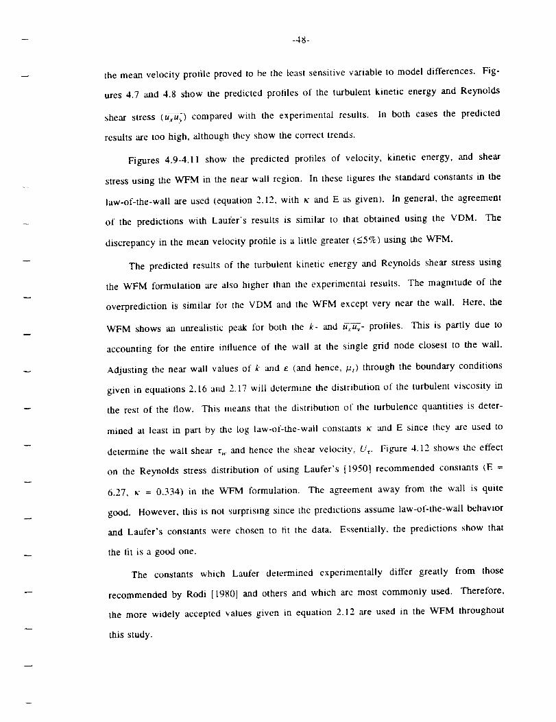
-48-
the mean velocity profile proved to be the least sensitive variable to model differences. Fig-
ures 4.7 and 4.8 show the predicted proliles of the turbulent kinetic energy and Reynolds
shear stress (U_y) compared with the experimental results. In both cases the predicted
results are too high, 'although they show the correct trends.
Figures 4.9-4.11 show the predicted profiles of velocity, kinetic energy, and shear
stress using the WFM in the near wall region. In these tigures the standard constants in the
law-of-the-wall are used (equation 2.12, with _c and E as given). In general, the agreement
of the predictions with Laufer's results is similar to that obtained using the VDM. The
discrepancy in the mean velocity profile is a little greater (<5%) using the WFM.
The predicted results of the turbulent kinetic energy and Reynolds shear stress using
the WFM formulation are also higher than the experimental results. The magnitude of the
overprediction is similar for the VDM and the WFM except very near the wall. Here, the
WFM shows an unrealistic peak lor both the k- and uxu v- profiles. This is partly due to
accounting for the entire influence of the wall at the single grid node closest to the wall.
Adjusting the near wall values of k and e (and hence, pf) through the boundary conditions
given in equations 2.16 and 2.17 will determine the distribution of the turbulent viscosity in
the rest of the flow. This means that the distribution of the turbulence quantities is deter-
mined at least in part by the log law-of-the-wall constants _: and E since they are used to
determine the wall shear r_,. and hence the shear velocity, Us. Figure 4.12 shows the effect
on the Reynolds stress distribution of using Laufer's [1950] recommended constants (E =
6.27, _, = 0.334) in the WFM formulation. The agreement away from the wall is quite
good. However, this is not surprising since the predictions assume law-of-the-wall behavior
and Laufer's constants were chosen to fit the data. Essentially. the predictions show that
the fit is a good one.
The constants which Laufer determined experimentally differ greatly from those
recommended by Rodi [1980] and others and which are most commonly used. Therefore,
the more widely accepted values given in equation 2.12 are used in the WFM throughout
this study.

- -49-
The overprediction of the turbulence quantities in the core of the flow by both model
formulations is due, in part, to assumptions implicit in the models themselves. The k-e
model assumes local isotropy of the normal stresses when, in fact, the streamwise lluctua-
tions in the channel flow are up to five times greater than the cross-stream fluctuations.
This is certain to al_fect both the predicted k-profile as well as the UxUv-profile, which is
related to the kinetic energy through the Boussinesq assumption (equation 2.14).
Figures 4.13-4.16 and 4.17-4.20 compare results obtained with the VDM formulation
with those obtained using the WFM lormulation (and standard constants). The first set of
four figures gives the profiles obtained when the overlap region between the VDM and HRE
regions is located at v+=10. It will be seen that the agreement obtained for the velocity
profile and the k- and e- profiles is fairly close. The agreement of the profiles of the tur-
bulence quantities yields agreement in the profile of the effective eddy viscosity shown in
Figure 4.16. In contrast with this close agreement between predictions using the two model
formulations, the differences in Figures 4.17-4.20 are larger. The VDM predictions in this
case were made by fixing the overlap region between the near wall and the core flow at
y+=25. The mean velocity profile in Figure 4.17 shows the least sensitivity to this change,
although the discrepancies are larger than those in Figure 4.13. Figures 4.18-4.20 show
large differences in the profiles of k and e and in the resulting effective eddy viscosity
profile. Locating the near wall/core overlap region too far from the wall can be seen to
have a significant effect on determining the distribution of the turbulence quantities, and
hence on the effective turbulent transport properties. Additional tests with the overlap
region located still further from the wall region led to further discrepancies in the tur-
bulence quantity profiles. As a result of these comparisons, prior to making the detailed
curved duct calculations using the VDM, some preliminary coarse grid calculations were
made to determine the grid positions in wall coordinates. The overlap region was then
chosen to occur in the region y+=10-15.
Developing flow in a square duct. Figures 4.21-4.28 show comparison of calculated
results with the experiments of Melling [1975]. The calculations were conducted in one
half-plane of the duct cross-section to take advantage of a plane of symmetry in the

-50-
geometricalconfiguration.Calculations could have been pertbrmed in one quadrant of the
duct since there are actually two planes of symmetry in straight duct flow. This was not
done since the resulting fully developed duct proliles were to be used as the inlet flow for
the curved duct calculations where there is only one plane of symmetry. As in the straight
channel calculations the profiles were determined to be fully developed when they exhibited
no further change in the streamwise direction. Further. the streamwise pressure gradient
and wall shear stress were constant.
The calculations were performed either on a non-uniform 25 x 50 x 40 (z x y x x) grid
for the VDM formulation or a non-uniform 20 × 40 x40 (z x y x x) grid for the WFM for-
mulation. The 40 planes in the streamwise (x) direction corresponded to approximately
25Dh, which was not enough to yield a fully developed solution. The outlet profile was
therefore used as an inlet profile and another 25D h were calculated in the streamwise direc-
tion. This process was continued until no changes were observed in the profiles of velocity
and the turbulence quantities. The grid distribution was determined from the preliminary
turbulent channel flow calculation where the significant flow features were found to be well
resolved.
The development of the centerline velocity for the WFM and VDM calculations are
compared with Melling's [19751 data in Figures 4.21 and 4.22, respectively. The develop-
ment of the streamwise turbulence intensity, is shown for the WFM and VDM calculations
in Figures 4.23 and 4.24. The turbulence intensity was determined from the k-e model and
is related to the root mean square of the velocity fluctuations, ii. If local isotropy is
assumed, then the r.m.s, velocity is
_= = 3k(4.1)
The turbulence intensity is determined either as a percentage of the bulk velocity, Ub or the
centerline velocity, Uct as in Melling's experiments:
Intensity - _" .100 (4.2)U,I
Because of the isotropic viscosity assumption, all three components of the calculateu

-51-
turbulence intensity are identical. Comparisons with Melling's data are made with the
measured streamwise turbulence intensity.
Melling had a smooth square contraction upstream of the duct and used a boundary
Layer trip at the duct entrance. Because he used a boundary layer trip in his experiments,
the initial conditions are difficult to reproduce numerically. Instead a virtual origin for the
calculations is determined by adjusting the axial location of the experimental profiles so that
they agree with predictions at some initial position. In this case the virtual origin was
determined to be about 6Dh upstream of the trip. The protiles in Figures 4.21-4.24 have
been adjusted to account for this experimental virtual origin.
The development length of turbulent duct flow in a square cross-section duct varies
between 85Dh and 140Dj, depending on the inlet conditions, according to Demuren and
Rodi [1984]. Although the basic features of the fully developed duct flow are present in
Melling's measurements at the last streamwise measurement position, an additional 40-50
hydraulic diameters would be necessary to obtain a truly fully developed flow. Even at the
final downstream measurement position (36.8 Dja from the entrance) the flow was far from
being fully developed. Melling [1975] mentioned that the centerline velocity and tur-
bulence intensity were still changing at the final measurement station, although the changes
observed were small. For the WFM calculations (Figure 4.2l) the development length was
approximately 70Dh, while tot the VDM calculations (Figure 4.22) the length was a little
longer, approximately 90D h. These values compare well with those determined by
Demuren and Rodi [1984]. It is clear from the figures that the experimental profiles do not
exhibit as large a variation in the centerline velocity and turbulence intensity as the calcula-
tions show.
There is a noticeable overshoot in the predicted profiles of velocity and turbulence
intensity using either of the model formulations ( the "hump" in the Figures). A similar
overshoot was noted by Melling in the experimental study, although much smaller in mag-
nitude and occurring earlier in the development region. This was due to a redistribution of
the momentum in the duct by the Reynolds stress driven secondary motion. In the numeri-
cal calculations this type of secondary motion will not occur because of the assumed

isotropy of the eddy diffusivity term, vt. However, a redistribution of momentum by means
of the turbulent diffusion probably does influence the centerline profiles of velocity and tur-
bulence intensity. For example, the turbulence intensity profiles of Figures 4.23 and 4.24
show a much longer development length before the turbulence intensity starts to increase.
This could be explained by the transport due to turbulent diffusion being underpredicted m
the initial development region of the duct. This would account for the longer length over
which the centerline velocity increases, since the low value of k at the centerline would
lead to less mixing in this region. When the centerline turbulence intensity increases in
both model tbrmulations there is an accompanying decrease in the centerline velocity.
Figure 4.25 compares experimental and numerical contours of the streamwise velocity
for fully developed flow in a square duct. The experimental results are from Melling's
[1975] study, at the final downstream measurement plane. As mentioned earlier the experi-
mental profiles still showed evidence of further downstream development, but the changes
were small (<_1%). The bulging in the experimental contours towards the duct corners are
due to the stress driven secondary motion referred to above. These "bulges" do not show
up in either of the predictions because of the isotropic eddy diffusivity assumption of both
model formulations. Figure 4.26 shows the streamwise velocity profile at two cross-stream
positions. The profiles were taken at the symmetry, plane t z/D_, = 0.5) and midway between
the symmetry plane and duct wall (z/Dh = 0.25). The profiles indicate the symmetry which
exists in the flow both experimentally and numerically. There is little difference in the
predicted results using either model formulation, the agreement being to within 1%. The
discrepancies between the measured and predicted profiles are due primarily to the absence
of stress driven secondary motion in both calculation schemes. This secondary motion
results in a flatter velocity profile in the core of the duct flow and steeper velocity gradients
in the comers than predicted.
Figures 4.27 and 4.28 show similar contour and profile comparisons tbr the streamwise
turbulence intensity. The "bulging" towards corners is sharper than that occurring in the
velocity contours and again does not show up in the computations.

- -53-
The VDM calculationshowsa higherturbulenceintensityin thecoreof the flow and
not as sharpa drop-off in the cornersasthe WFM predictions.The flatterprofile in the
cornerregionsin the VDM resultsis likely du_' _ thecornertreatmentin calculatingthe
eddyviscosityfor the mixing lengthmodel. In the mixing lengthregion(seeFigure2.3),
the distancefrom the wall tY) used in equalions 2.21, is an effective length determined
from"
l le_1_1f = z2y _-
z2 + y., (4.3)
where z and y are perpendicular distances from the neighboring walls. Far from a second
w_l, this reduces to l,,yf = "_ or le8 = Y, depending on which wall is nearest. In a corner
t'"
region where z = y, equation 4.3 gives l<f = :/_12. This in turn gives a smaller mixing
length, which results in a lower estimate of the eddy diffusivity and a flatter profile of the
turbulence intensity. The effect of the corner treatment is not limited to the mixing length
region but is also felt in the HRE core region through the boundary conditions for k and tr
in the overlap region. This can be seen in the contours of Figure 4.27 and the profiles of
Figure 4.28. In the latter figure, a comparison of the predicted profiles using the VDM for-
mulation in (a) and (b) shows a flatter prolile in (b) which is located halfway between the
second wall and the symmetry plane. A comparison of the profiles predicted in Figure 4.28
shows that the VDM formulation predicts a turbulence intensity about 1% higher than the
corresponding WFM predictions throughout the core of the flow. Only in the near wall
region does the WFM prediction of E/U,t exceed that of the VDM predictions. The peaks
which occur in the predictions using the WFM are a result of the log law-of-the-wall boun-
dary conditions (equation 2.18) used in the near wall region for this formulation. They lead
to steep gradients of k in this region which are not supported by the experimental data.
4.4. Conclusions
The semi-elliptic calculation procedure has proved to be
predicting the developing laminar flows presented in this chapter.
be stably applicable for turbulent flow calculations.
numerically accurate in
It has also been shown to
Here, where numerical discrepancies
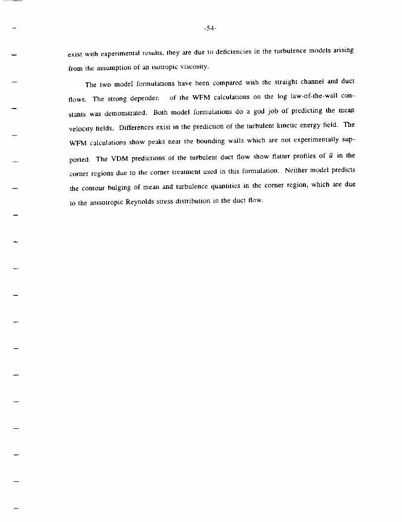
- -54-
exist with experimental results, they are due to deficiencies in the turbulence models arising
from the assumption of an isotropic viscosity.
The two model formulations have been compared with the straight channel and duct
flows. The strong depender, of the WFM calculations on the log law-of-the-wall con-
stants was demonstrated. Both model formulations do a god job of predicting the mean
velocity fields. Differences exist in the prediction of the turbulent kinetic energy field. The
WFM calculations show peaks near the bounding walls which are not experimentally sup-
ported. The VDM predictions of the turbulent duct flow show flatter profiles of _ in the
corner regions due to the corner treatment used in this formulation. Neither model predicts
the contour bulging of mean and turbulence quantities in the corner region, which are due
to the anisotropic Reynolds stress distribution in the duct flow.

-55-
5. RESULTS AND DISCUSSION
5.1. Introduction
Predictions of the turbulent flow in a 90 ° bend ,are presented in this section. The cal-
culalions were performed using the two equation k-e model in the core of the flow and
either wall functions {WFM) or the Van Driest mixing length model (VDM_ in the near
wall region. As was mentioned in the previous section the isotropic viscosity assumption
prevents the prediclion of the stress-driven secondary motion that occurs in straight duct
turbulent flow. However, in a bend one expects the much larger pressure-centrifugal force
driven secondary motion to exceed, by a large amount, the stress-driven motion that is dom-
inant in straight duct flows. Therefore, the assumption of an isotropic viscosity may be less
critical to resolving the main features of the bend flow. T'he calculations were made using
the semi-elliptic code described above, employing 65 planes in the streamwise direction.
There were 45 planes used to resolve the flow in the bend itself, and 10 planes to resolve
the flow in each of the straight duct tangents. The streamwise planes were distributed uni-
formly, every 2 ° in the bend. This distribution was sufficient to resolve the steady state
structures appearing in the bend. A contracting grid was used in the streamwise direction in
the upstream tangent while an expanding grid was used in the downstream tangent. This
meant that the greatest resolution in the tangents occurred where they joined the 90 ° bend.
In the cross-stream planes a non-uniform 20×40 (: x r) grid was used for the WFM calcu-
lations and a non-uniform 25 × 50 (: x r) grid for the VDM calculations. This grid distri-
bution corresponds to that used to make the straight duct turbulent calculations discussed in
the previous section. The grids are shown in Figure 5.1.
Much of the testing of the code discussed in Chapter 4 was done on the campus IBM
3090 main-frame computer. The final production runs for the curved duct calculations were
performed on a CRAY-XMP supercomputer. The calculations of the 90 ° bend proved to be
prone to instabilities in the pressure field even when using all of the stabilizing techniques
discussed in Chapter 3. This is most likely due to the strongly elliptic nature of the flow
field in a bend with a small radius of curvature. The calculations for both model formula-
tions required 400 passes to obtain a converged solution. For the WFM predictions this
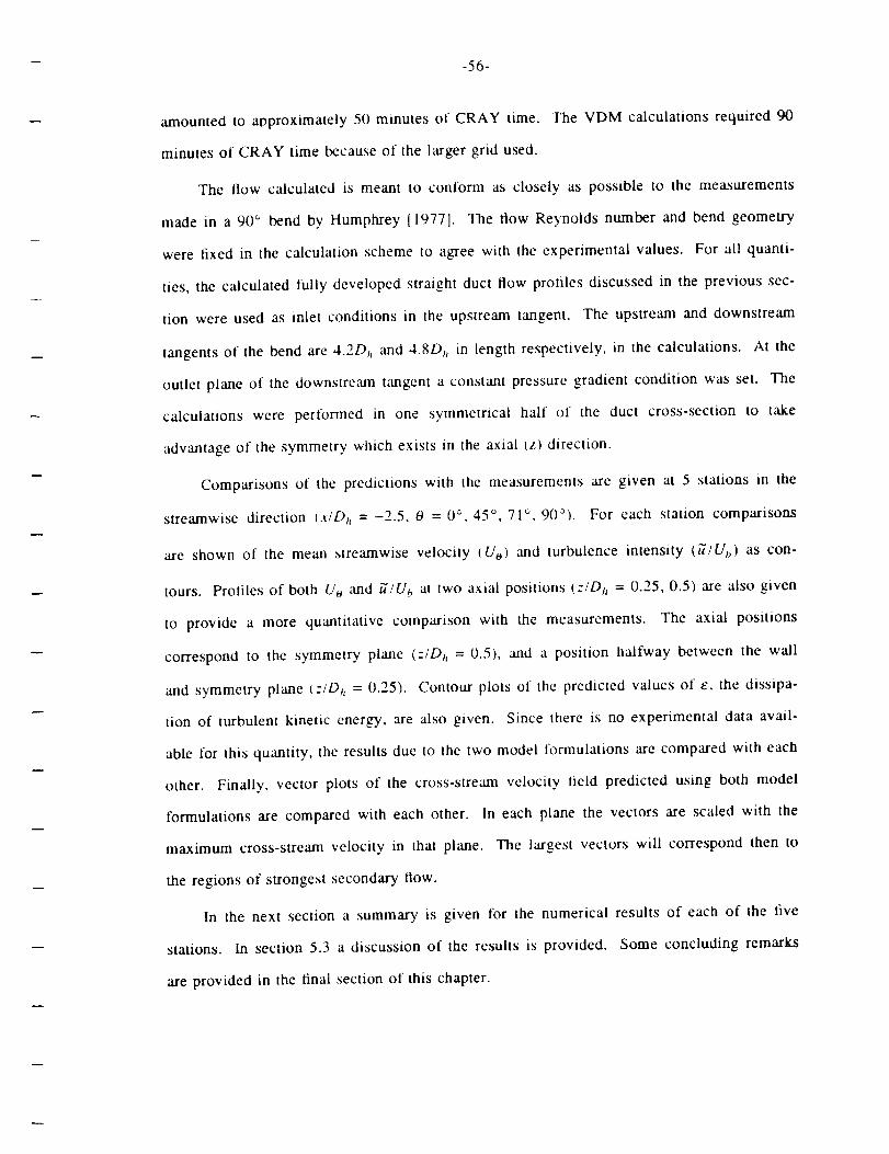
-56-
amountedto aoproximately50 minutesof CRAY time. The VDM calculationsrequired90
minutesof CRAYtimebecauseof the largergrid used.
The flow calculatedis meantto conform as closely as possible to the measurements
made in a 90 ° bend by Humphrey 11977]. The flow Reynolds number and bend geometry
were fixed in the calculation scheme to agree with the experimental values. For all quanti-
ties, the calculated fully developed straight duct flow profiles discussed in the previous sec-
tion were used as inlet conditions in the upstream tangent. The upstream and downstream
tangents of the bend are 4.2Dj, and 4.SDh in length respectively, in the calculations. At the
outlet plane of the downstream tangent a constant pressure gradient condition was set. The
calculations were pertbrmed in one symmetrical half of the duct cross-section to take
advantage of the symmetry which exists in the axial _z) direction.
Comparisons of the predictions with the measurements are given at 5 stations in the
streamwise direction I.t/D_, = -2.5, 0 = 0 °, 45 °, 71 °, 90°). For each station comparisons
are shown of the mean streamwise velocity (Us) and turbulence intensity ('_/Uh) as con-
tours. Proliles of both Uo and "ff/U b at two axial positions (z/Dj, = 0,25, 0.5) are also given
to provide a more quantitative comparison with the measurements. The axial positions
correspond to the symmetry plane (z/D h = 0.5), and a position halfway between the wall
and symmetry plane {:/D h = 0.25). Contour plots of the predicted values of e. the dissipa-
tion of turbulent kinetic energy, are also given. Since there is no experimental data avail-
able for this quantity, the results due to the two model lormulations are compared with each
other. Finally, vector plots of the cross-stream velocity field predicted using both model
formulations are compared with each other. In each plane the vectors are scaled with the
maximum cross-stream velocity in that plane. The largest vectors will correspond then to
the regions of strongest secondary flow.
In the next section a summary is given /or the numerical results of each of the five
stations. In section 5.3 a discussion of the results is provided. Some concluding remarks
are provided in the final section of this chapter.
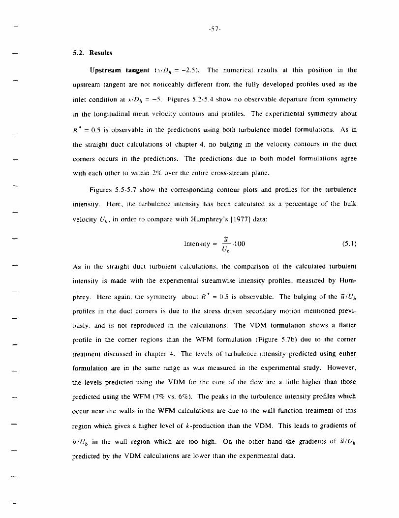
w -57-
5.2. Results
Upstream tangent tx/Dh =-2.5). The numerical results at this position in the
upstream tangent are not noticeably different from the fully developed profiles used as the
inlet condition at x/Dh = -5. Figures 5.2-5.4 show no observable departure from symmetry
in the longitudinal mean velocity contours and profiles. The experimental symmetry about
R* = 0.5 is observable in the predictions using both turbulence model formulations. As m
the straight duct calculations of chapter 4, no bulging in the velocity contours in the duct
comers occurs in the predictions. The predictions due to both model formulations agree
with each other to within 2% over the entire cross-stream plane.
Figures 5.5-5.7 show the corresponding contour plots and profiles for the turbulence
intensity. Here, the turbulence intensity has been calculated as a percentage of the bulk
velocity Uh, in order to compare with Humphrey's [1977] data:
Intensity = u_.100 (5.1)Ub
As in the straight duct turbulent calculations, the comparison of the calculated turbulent
intensity is made with the experimental streamwise intensity profiles, measured by Hum-
phrey. Here again, the symmetry about R* = 0.5 is observable. The bulging of the "ff/U b
profiles in the duct corners is due to the stress driven secondary motion mentioned previ-
ously, and is not reproduced in the calculations. The VDM formulation shows a flatter
profile in the comer regions than the WFM formulation _Figure 5.7b) due to the comer
treatment discussed in chapter 4. The levels of turbulence intensity predicted using either
formulation are in the same range as was measured in the experimental study. However,
the levels predicted using the VDM tor the core of the flow are a little higher than those
predicted using the WFM (7% vs. 6%). The peaks in tile turbulence intensity profiles which
occur near the wails in the WFM calculations are due to the wall function treatment of this
region which gives a higher level of k-production than the VDM. This leads to gradients of
"ff/Ub in the wall region which arc too high. On the other hand the gradients of _IU b
predicted by the VDM calculations are lower than the experimental data.
Figure 5.8 compares the predicted contours of e, the dissipation of turbulent kinetic
energy using the two Iormulations. In the core of the Ilow the dissipation levels are very
similar. The contour lines are more "rounded" in the corners using the VDM formulation
tFigure 5.8b) due to the comer treatment used but the differences are small. It is in the
wall region that the differences are most notable. Here the dissipation level is five times
greater tor the WFM calculations than for the VDM calculations. The peak in the e-profile
is similar to that in the k-profile predicted in the WFM calculations.
0 = 0 ° plane. At the inlet plane the bend has definitely influenced the flow structure
development, both in the experiments and predictions. Figures 5.9-5.1 1 show an accelera-
tion of the fluid near the inner radius wall (r,) responding to the favorable streamwise pres-
sure gradient in this region. At the same time the fluid near the outer radius wall is
decelerated, responding to the unfavorable pressure gradient in this region. Both the model
formulations show this shift of the maximum velocity towards the inner radius wall. The
WFM lormulation predicts a slightly larger value of the velocity maximum than the VDM
lbrmulation. This is shown further in Figure 5.15, the vector plot of the cross-stream velo-
cities for both models. Here all the radial velocities in both cases are from the concave
outer wall towards the convex inner wall. This streamwise pressure gradient distribution at
the inlet plane is caused by the centrifugal force-radial pressure gradient imbalance set up in
the llow downstream in the bend. The centrifugal forces acting on the fluid in the bend
itself do not influence the flow at the inlet plane. The resulting acceleration near the inner
radius wall is similar to what would happen to an inviscid flow in the bend.
The bulging of the velocity prolile towards the corner at the inner radius wall, which
is exhibited in the experiments, is a residual of the stress-driven secondary motion so it
does not show up in the predictions. The same effect appears in Figure 5.11b as an
underprediction of the maximum velocity in the region near r,. The differences in the pred-
ictions of the mean velocity lield by the two model formulations are small throughout the
entire cross-section.
In Figures 5.12-5.14 contours and proliles of the turbulence intensity are given. The
experimental results show small but noticeable changes in the "_/Ub profiles. The

-59-
predictionsof both model lbrmulations show larger variations from the upstream tangent
station, even at this early point in the bend. Both sets of calculations show a shift towards
the inner radius wall of the intensity contours in response to the favorable pressure gradient
near ri and the unfavorable pressure gradient near r,. The shift is similar to that displayed
by the Uo profiles in Figures 5.8-5.10 and can also be seen in the experimental profiles.
The WFM calculations show a large increase in the maximum turbulence intensity
(26%) near the inner radius wall over lhe peak value in this region at the upstream tangent
location (17%). There is a corresponding drop-oft in the intensity peak near the outer
radius wall. The WF/Vl predictions correspond to a large increase in the production of tur-
bulent kinetic energy near r, and a drop-off in production near to. The VDM calculations
show a much smaller change in the kinetic energy production in both regions. In the core
of the flow, the g/U_, protiles predicted by the VDM calculations is 1%-2% higher than
those predicted by the WFM calculations (Figure 5.14).
The predicted contours of energy dissipation, e due to both model formulations are
compared in Figure 5.16. There is a small shitt of the constant e contours towards the
inner radius wall shown by both sets of calculations. The dissipation contours show a simi-
lar asymmetry to that shown in the turbulence intensity profiles (see Figures 5.12 and 5.13).
Since the regions of high turbulence intensity correspond to regions of increased energy dis-
sipation, the contours of both quantities often show similar behavior. The WFM predictions
show a higher dissipation level near r, due to the higher production of k. In the core of the
flow the predicted values show small variations depending on the model formulations.
0 = 45 ° plane. The acceleration of the flow near the inner radius wall is also notice-
able at the 45 ° plane. This shows up in Figures 5.17-5+19 in the contours of Uo which are
displaced towards the convex inner wall. The predictions of both model formulations yield
similar contour plots, shown in Figures 5.17 and 5.18. However. the predicted radial
profiles of Uo in Figure 5.19 show some quantitative variations between the results of the
two models. In this figure the results of the WFM and VDM calculations of this study are
compared with the numerical results of Humphrey et al. [1981] in addition to the experi-
mental results of Humphrey [1977]. The calculations of Humphrey et al. used an elliptic

- -60-
procedure and a coarse grid, I1 x 14x 19 (x x r x O) with wall functions in the near wall
region. In general, the results of the VDM and WFM calculations are in agreement with
each other. The VDM formulation does a better job of predicting the velocity profile near
the inner radius wall on the symmetry plane eFigure 5.19a) but both models as well as the
elliptic calculations miss the velocity peak and drop-off near the outer radius wall. At the
=/D h = 0.25 position (Figure 5.19b) both WFM and VDM are in better agreement with the
data (particularly in the region near r,,) than the elliptic calculations of Humphrey et al.
[19811.
At the 45 ° plane, the secondary motion in the cross-stream plane begins to be notice-
able. The predicted contours of Uo in Figures 5.17 and 5.18 show the beginnings of the
deformation due to the secondary flow which is already evident in the experimental results.
Figure 5.23 shows the predicted cross-stream velocity vector plots. In the figure the longi-
tudinal vortices characteristic of bend flow are clearly evident. Both sets of calculations
show a relatively thin layer (0.15D h) of fluid moving quickly along the side wall of the
bend from the concave outer radius wall towards the inner radius wall. The slower moving
fluid in the core of the flow moves from r, to r,, forming a stagnation region on the sym-
metry plane at the outer wall. There are some distinct differences in the predictions of the
streamwise vortices based on the two models. For example, the centers of the predicted
vortices (where the cross-stream velocity is zero) have different radial locations. The VDM
c',dculations predict the zero velocity location to be at R* = 0.55 (Figure 5.23a) while the
WFM predictions give R'= 0.35. much closer to r,. In addition, the maximum cross-
stream velocity predicted by the WFM formulation was Ur = 0.5U_ while the VDM formu-
lation only gave cross-stream velocities as high as U,. = 0.38Uh. In both cases the max-
imum velocities occurred near the flat side walls in the pressure dominated side wall boun-
dary layers.
Figures 5.20-5.22 show the contours and profiles of the turbulence intensity, "ff/U b
compared with the experimental results. Although the details of the ff/Ub distribution are
not reproduced by the predictions, many of the qualitative features emerge. Both sets of
calculations show high levels of u/Ui, (12_-14%) near the outer concave wall and near the
flat side wall compared to the inner convex wall (8%-9%). These values of turbulence
intensity are similar to the values found in the experiments though the contour shapes are
different. In comparing the predictions of the two model formulations in Figure 5.22, the
peaks in the normal stress proliles predicted by the WFM appear near the inner and outer
radius walls. In the core of the flow the VDM calculalions predict slightly higher values of
the intensity than the WFM calculations. As before, qualitative features in the dissipation
profiles similar to the turbulence intensity profiles show up in Figure 5.24.
0 = 71 ° plane. At this position in the bend the influence of the centrifugal force on
the fluid (through the cross-stream secondary motionl finally manifests itself in the stream-
wise velocity profiles. The contours of U o are shown lbr the two sets of calculations in
Figures 5.25-5.27. The maximum velocity has been displaced to the outer radius wall on
the symmetry plane tFigurc 5.27a). Both model formulations predict a greater shift (to
R" -- 0.55) than shows up in the experiments. The VDM calculations are in better agree-
ment with the experimental profiles in Figure 5.27 in the region near the inner convex wall
(0 < R" _< 0.5). Both models miss the drop-off in the velocity profile near %. The ten-
dency of the U u contours to bend in the corners near r, is more prevalent in the WFM cal-
culations and is probably due to the different secondary flow patterns predicted there, shown
in Figure 5.31. Differences in the predicted vector plots similar to those found at 0 = 45 °
show up again. In particular, the location of the zero cross-stream velocity is closer to the
fiat side wall and convex inner wall in the WFM calculations (Figure 5.31b) than in the
VDM calculations (Figure 5.31a). This is consistent with a higher radial velocity in the
side wall boundary layers in the WFM results and leads to a greater deformation in the
longitudinal velocity contours. In both sets of predictions the movement of the zero velo-
city point is towards r i from the 45 ° plane to the 71 ° plane. The maximum cross-stream
velocities predicted by the WFM formulation are U r = 0.5 U b in the region near the flat side
walls and Ur = 0.4Ub in the VDM tormulation, ",.dso near the side walls.
Figures 5.28-5.30 show the predicted distribution of the turbulence intensity. Here
again, there is qualitative agreement with the experiments although many details ,are not
reproduced numerically. At this position in the bend the turbulence intensity is still highest
-- -62-
neartheconcaveouterwall andflat sidewalls (12%-!4%). However,the intensitylevelsin
the regionof r i have increased t=9%) compared to this region at 0 = 45 ° . The trend of
increasing turbulence intensity near r, is also noted in the experimental contours and
profiles. The same peaks in the "ff/Uh profiles near the walls in the WFM calculations again
show up, as does the slightly higher turbulence level in the core of the flow, also predicted
the VDM calculations.
Figure 5.32 shows the predicted contours of the energy dissipation e, due to the two
sets of calculations. The features in both cases are very similar. The relative peaks of e
near the bounding walls is in keeping with the fact that the maximum dissipation occurs in
the regions of maximum k production. The higher relative values of e in the very near wall
region of the WFM calculations are due to the wall function boundary conditions employed
in the WFM formulation.
0 = 90 ° plane. At the exit plane of the bend there are some fairly drastic differences
between the predicted velocity fields and the experimentally measured one. Figures 5.33-
5.35 compare the predictions with Humphrey's [1977] experimental results at this plane and
also with the clliptic calculations of the flow by Humphrey et al. [1981]. The predicted
location of the velocity maximum on the symmetry plane was R * = 0.9 in both model c',d-
culations as compared with the experimental location of R' = 0.57. The influence of the
secondary motion on the streamwise velocity contours ts more pronounced in the WFM
results than in the VDM results. Both model formulations of the present study show the
drop-off in Uo near r, on the symmetry plane. This feature is completely m_ssed by the
elliptic calculations of Humphrey et al. [ 1981 ].
The predicted cross-stream velocity fields shown in Figure 5.39 continue to exhibit the
same qualitative differences which are dependent on the model formulation. The zero velo-
city point has moved tow,'uds the inner radius wall in both cases and has moved away from
the side wall towards the symmetry ptane in the WFM predictions. The maximum cross-
stream velocities predicted by the WFM calculations are Ur = 0.36Ub in the region near the
fiat side walls. Velocities of up to U,. = 0.24Uh are predicted on the symmetry plane. The
VDM calculations yield maximum radial velocities of Ur = 0.3Ub near the side walls and

-- -63-
U r = 0.28Uh on the symmetry plane. In Humphrey's [1977] experimental study the max-
imum radial velocities occurred on the symmetry, plane _U_ = 0.28Uh). The maximum
radial velocities Humphrey measured near the side walls were Ur ---0.14U b. Both models
show evidence of small secondary longitudinal vortices near r,, on the symmetry plane.
These are induced by the primary vortices and much weaker in strength. These secondary
vortices were not discussed in Humphrey's experimental investigation but may have been
present.
Figures 5.36-5.38 show the predicted turbulence intensity (_/Uh) profiles compared
with Humphrey's data. The effect ol I the strong cross-stream velocity field can be seen in
the calculated _/U b distribution. There is a decrease in the predicted turbulence intensity
near the outer concave wall (to 10%-12%) and a corresponding increase near the inner con-
vex wall (9%-10%) relative to the 71 ° plane. The peak in turbulence intensity near the side
wall has also moved from r, towards rl in both sets of calculations. These trends are simi-
lar to those found in the experiments, although the turbulence levels, particularly near ri,
are significantly higher than those predicted using either model formulation (12% vs. 8% in
Figure 5.38a). The VDM calculations predict turbulence levels 2%-3% higher than the
WFM calculations away from the walls. Neither model picks up the local minimum in the
normal stress distribution. The predicted proliles tend to be llatter and show less variation
in the radial direction than is experimentally observed (Figure 5.38).
The same trends in the predictions of ?i/Uh are observable in the contour plots of the
energy dissipation, _ in Figure 5.40. The dissipation peaks near those walls where the pro-
duction of k is highest and decreases towards the core of the llow. Both models predict
increasing dissipation levels near the inner radius wall as compared to the 71 ° plane (com-
pare Figure 5.32 and 5.40). The contours also show the effect of the cross-stream velocity
field in the bending of the contour lines near r,. The high levels of energy dissipation very
close to the walls predicted by the WFM formulation are not found in the VDM calcula-
lions.
Figure 5.41 shows the variation of the pressure coelficient ce, on the duct symmetry
plane at the inner and outer radius walls, where
- -64-
ApCp --
'_p U;
Since there is no experimental data with which to compare the predictions, the results of the
two model formulations are again compared with each other.
Qualitatively, the two models predict similar variations in the pressure coefficient.
Both show the favorable pressure gradient at r, and the adverse gradient at r,, near the bend
entrance. This is responsible lot the relative fluid acceleration in the region near r i
upstream of the bend. The pressure gradients predicted by both models near the bend exit
are also in agreement with each other. On the intter radius wail. the largest variation
between between the two models occurs at the minimum value of cp at 25 c' in the bend.
Here, the difference in the predicted values of the pressure coefficient is 5,'76 of the dynamic
pressure, l/'-pU_. On the outer radius wall, the largest variation occurs at the maximum
value of _'p at 58 ° in the bend. The difference in the predicted values of ct, is also 5% of
the dynamic pressure.
The maximum aJld minimum values of _t, do not occur at the same longitudinal (0)
position in the bend as was found in the experimental investigation of a 90 ° bend by Taylor
et ai. [1982]. This could be due to the different inlet conditions in the experiments which
had thin boundary layers on the side walls upstream of the bend. Unlbrtunately, for the
case modeled in the present work, Humphrey did not provide data for the pressure field
variation in the bend.
The bend also apparently affects the pressure fields in the straight duct tangents. The
influence of the bend on the pressure field in the upstream duct tangent extends 1.5Dh
upstream of the bend entrance. In the downstream tangent, the effect of the bend is still
noticeable 3Dh after the bend exit plane.
The variation of the friction coefficient Q. on the symmetry plane at the inner and
outer radius walls is shown in Figure 5.42, where

-65-
Cf --
imp U_
Despite qualitative simil,-u'ities, there are some fairly h'uge differences in the predictions of
the two model formulations. The initial differences in the friction coefficient upstream of
the bend are due to the different near wall model formulations. This initial difference might
be expected to persist through the bend, however, this is not the case. The differences are
most pronounced near the bend entrance on the inner radius wall and near the bend exit on
the outer radius wall. These are regions where the maximum shear stress occurs on the
radial walls. A comparison wiih Figure 5.41 shows that these regions are where favorable
pressure gradients exist, which cause the fluid to accelerate in the streamwise direction.
The WFM formulation shows larger changes in the friction coefficient in these regions. The
differences between the two models amounts to t0% of the dynamic pressure, l/2pU_ at the
bend inlet and 17% at the bend exit. Both model formulations agree on the streamwise
locations of the local maxima in the friction coefficient profile. On the inner radius wall the
maximum occurs at I ° into the bend, while at the outer radius wall it occurs 0.4D#, down-
stream of the bend exit in the downstream tangent.
The models are in closer agreement in predicting the location and magnitude of the
minimum friction coefficient in the bend. At the outer radius wall, Q reaches its minimum
value at 10 ° into the bend. The difference in the predictions of the two models here is 1%
of the dynamic pressure. Of more interest is the local minimum which occurs at r i. Here
the minimum value of t'f occurs in the downstream tangent, 0.3Dh beyond the bend exit,
where it goes to zero. This indicates a potential at this location lor streamwise recirculation
which is no,_ ermitted in the semi-elliptic calculation scheme. The streamwise diffusion
terms in the momentum and turbulence equations (underlined in equations 2.26-2.30) have
been neglected, although in this region they are certainly important. To get an accurate
description of the flow field in this region, a fully elliptic procedure would have to be used,
Downstream of the bend exit the two models predict a return to the straight duct
values of t'f although at 3.5Dh in the downstream tangent the flow is still developing.

-66-
5.3. Discussion
A comparison of the predicted results with the experimental data lot the turbulent flow
in a 90 ° bend shows similar qualitative behavior throughout the bend. There are some
quantitative differences which exist, particularly in the distribution of the turbulent kinetic
energy, k. In general, both model formulations predicted the overall features of the flow,
although the results differed in some details. The acceleration of the liow near r, between
the bend inlet and the 45 ° plane, and the onset of secondary motion in the cross-stream
plane, were well predicted in both sets of calculations. The location of the velocity max-
imum near the center of the duct curvature up to the 0 = 71 ° plane, followed by a shift to
the outer concave wall was also predicted by both model formulations. The general
development of the turbulence intensity i//Uh field through the bend and its modification by
the cross-stream velocity field can be seen in the figures for 0 = 45 °, 71 ° and 90 °.
Some features of the flow do not show up at all in the calculations. The "bulging" of
the velocity and turbulence intensity profiles towards the duct corners does not show up in
the predictions of the upstream tangent and bend inlet plane positions. The bulging, due to
the Reynolds stress driven secondary motion in straight duct, cannot be predicted with a
model formulation which assumes an isotropic eddy diffusivity.
The development of the longitudinal vortices in both sets of calculations is slower than
in the experiments. As a result there is less distortion of the Uo profiles in the corners near
r i. The shift in the maximum turbulence intensity from r,, at 0 = 45 ° to r_ at 0 = 90 ° is
also not complete in either set of predictions compared with the experiments. As a result,
there is less slower moving fluid near the inner radius wall between 0 = 45 ° and 0 = 71 °
than is experimentally the case. This could be due to the predicted radial pressure gradients
being weaker than in the experimental study. This in turn, would favor the centrifugal
forces acting on the fluid and lead to a velocity maximum closer to the concave outer wall
than is actually the case IFigures 5.27 and 5.35).
The maximum secondary velocities predicted by the WFM calculations tend to be
higher than those predicted by the VDM formulation and higher than experimentally meas-
ured. In Humphrey's [19771 study the maximum radial velocity occurred at the outlet plane
-- -67-
on thesymmetryplaneandwas Ur = 0.28Ub. Both models predicted similar radial veioci-
lies at this position but also predicted radial velocities Ur = 0.3Uh near the side walls as
compared with Humphrey's measured values of Ur = 0.14U_,. The maximum calculated
cross-stream velocities occurred upstream at lhe 0 = 45 ° plane. The maximum predicted
velocities occurred near the flat side walls and were Ur = 0.4Uh and Ur --- 0.5Uh for the
VDM and WFM formulations, respectively.
The WFM formulation tcnds to predict much higher levels of turbulence near the
bounding walls than the VDM calculations due to the treatment of the wall region (see Fig-
ures 5.22. 5.30 and 5.38L In the WFM calculations the wall regions are treated using wall
functions as explained in Chapter 2. This method essentially fixes the maximum values of
k and e at the point nearest the wall and places all of the wall influence on the flow in the
determination of the boundary conditions for the dependent variables. The wall functions
were originally derived for a fully developed two-dimensional shear flow based on simple
equilibrium considerations. In the case of the flow in ducts and bends it leads to peaks in
the k- and e-profiles in the near wall region which have little experimental support.
The profiles of the pressure coefficient, ct, predicted by the two models at r i and %,
agree with each other quite well through the entire bend. In the predictions of the friction
coefficient, cf however, substantial differences exist. These are due to differences in the
near wall treatment of the two models as well as how they react to changes in the global
flow lield. Both models show a minimum value of c/ approaching zero near the bend exit
at the inner radius wall. This indicates the possibility of streamwise recirculation in this
region which cannot be handled by the semi-elliptic procedure.
Both model calculations do a better job of predicting the flow than the fully elliptic
calculations of Humphrey et ai. [1981}. This is almost certainly due to the coarse grid
llx14x19 (x x r x 0), used in the latter calculations and the resulting numerical diffusion.
An estimate of the magnitude of the numerical diffusion relative to turbulent diffusion is
given by the authors:
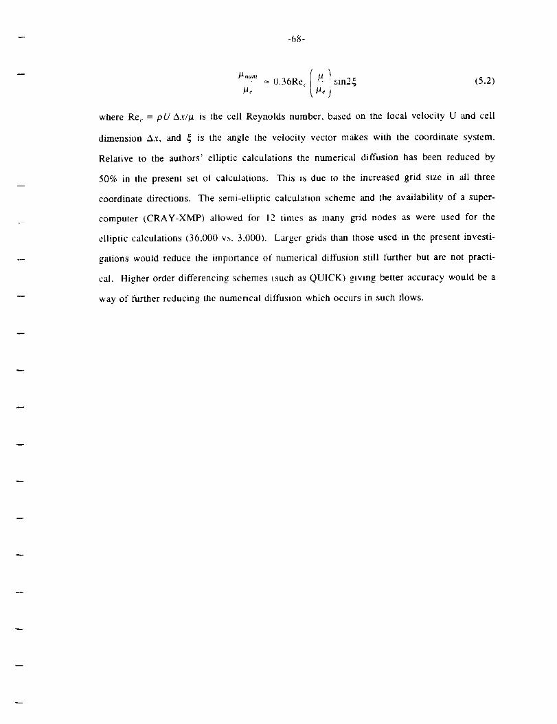
#1 rlum
.... 0.36Re, (5.2)
where Re<. = pU Ax//a is tlae cell Reynolds number, based on the local velocity U and cell
dimension Ax, and { is the angle the velocity vector makes with the coordinate system.
Relative to the authors' elliptic calculations the numerical diffusion has been reduced by
50% in the present set of calculations. This is due to the increased grid size in all three
coordinate directions. The semi-elliptic calculation scheme and the availability of a super-
computer (CRAY-XMP) allowed for 12 times as many grid nodes as were used for the
elliptic calculations (36,000 vs. 3,000). Larger grids than those used in the present investi-
gations would reduce the importance of numerical diffusion still further but are not practi-
cal. Higher order differencing schemes _such as QUICK) giving better accuracy would be a
way of further reducing the numerical diffusion which occurs in such flows.
-- -69-
6. CONCLUSIONS
Calculations of turbulent flow developing in a 90 _ bend of square cross section per-
formed using a semi-elliptic numerical procedure yield better results than earlier predictions
of the same flow using an elliptic procedure and a turbulence model equivalent to the WFM
of this work. This is attributed to the higher levels of grid refinement possible in the
present work.
Of the two models used here, the VDM shows better overall conformity with the
measurements of mean streamwise velocity. However, neither model reproduces well the
corresponding component of stress. This is clue to the assumption of an isotropic turbulence
viscosity in a flow where the convective, diffusive and pressure redistributions of a stress
field are important to resolve it properly. To improve upon this however, it would be
necessary to solve modeled transport equations for six stress components and such a task
was beyond the scope and resources available for this study. Notwithstanding, support for
this approach is to be found in the study by Choi et al [1987], brought to our attention at
the conclusion of the present work. These authors show that the use of an algebraic stress
model of turbulence, in conjunction with a semi-elliptic numerical procedure, yields consid-
erably improved predictions of the normal stresses for the flow in a 180 ° bend of square
cross section. Notwithstanding, improvements to predictions of the mean flow were fairly
minimal, substantiating the premise of this work, that the flow in a bend is dominated by
secondary motion of the tirst kind as a result of pressure-centrifugal force imbalances. The
correct calculation of the cross stream flow in a bend depends upon resolving accurately the
effects of the bend on the wall boundary layers. Wall-flow interactions, in the presence of
streamline curvature, represent the area of most pressing attention for the improved model-
ing of curved duct flows.

-70-
Appendix A
The QUICK scheme formulation
A.I The problem of interest
To achieve a stable higher order finite difference approximation of the convective
terms in the transport equations, that avoids the artilicial numerical diffusion caused by
upstream differencing and the unstable nature of central differencing, Leonard 11979] has
devised the QUICK (Quadratic Upstre,un Interpolation for Convective Kinematics) scheme.
This appendix outlines how the QUICK scheme is incorpt_rated in the REBUFFS code with
special consideration for the treatment required at boundaries.
A.2 Formulation
A.2.1 (;rid arrangement
The current REBUFFS code was programmed with the option for implementing
nonuniform grids. To simplify this outline, the grid arrangement for one direction only will
be discussed. With reference to Fig. A. 1 and A.2, for a nonuniform grid, passive properties
are located at locations x,, ,t,_, etc., and velocity nodes at .t,+,/,, and x;_, etc.. With this
grid arrangement, nodes for passive properties are always located inside the calculation
domain. A node surface will coincide with a boundary when the node is adjacent to the
boundary. Velocity nodes are placed halfway between two passive property nodes. This
kind of arrangement simplifies the coding process, especially for a multi-dimensional code.
For passive properties there is only one type of boundary node to consider, as shown in Fig.
A.3, while for velocities there are two, as shown in both Fig. A.3 and A.4, depending on
the velocity component considered.

-71-
A.2.2 Finite difference approximation of the convective termts)
The general convective term in the transport equations is represented by p_.V0 ,
where _ can be any passive property or velocity component. If the 0-transport equation is
expressed in divergence /or conservative) form, the convection terms can be represented as
V.{pUO). Integrating this expression over a one-dimensional linite control volume
enclosing node P as shown in Fig. A.I, yields the finite difference expression for the con-
vective term' (pu_),,A,, - tpu0 )_,Aw, where A represents the area at the subscripted inter-
face, and u is the velocity component in the direction considered. Since the _'s are not
defined on the interfaces, they have to be approximated by interpolation.
A.2.3 Quadratic upstream interpolation
Depending on the sign of the velocity component in question on each interface, the
grid points needed for interpolation vary. For example, with reference to Fig. A.I, assume
that both u_, and u_ are pt)sitivt?, i.e. directed in the positive x direction. In order to approx-
imate _w, we need _ at P, W, and WW. and for @, we need _ at E, P, and W. After the
interpolated values are found, they are substituted into the convective terms of the transport
equations. The difference equations are then expressed in terms of #'s that are defined at
the nodal locations. The interpolation equation used is _=ax"+bx+c. It is straightforward
to lind the coefficients in this interpolation equation.
Unfortunately, a direct application of the interpolation results to the convective terms
of the _-transport equation will not always guarantee convergence. This is because the
diagonal dominance of the resulting coefficient matrix is not necessarily guaranteed. In
order to devise a scheme that converges, Han et al. [1981] proposed a remedy that relies on
a "false transient" approach; i.e. placing some of the interpolation terms into the source
term in the difference equations. An improvement by Freitas et al. [1984] ensures that the
matrix of coefficients is diagonally dominant under all possible situations.
The procedure of Freitas el al. [1984] for setting up the finite difference expressions
tot the convective terms in a one-dimensional configuration is given below. The expressions
for C's in this appendix are different from the expressions derived by them. Their
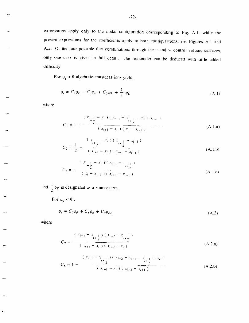
- -72-
expressions apply only to the nodal configuration corresponding to Fig. A.I, while the
present expressions for the coefficients apply to both configuralions; i.e. Figures A.I and
A.2. Of the four possible tlux combinations through the e and w control volume surfaces,
only one case is given in full detail. The remainder can be deduced with little added
difficulty.
For u e > 0 algebraic considerations yield,
1Oe "=" FlOp -- C2¢hE 4- C_Ow "4" _ qJE (A.I)
where
and
where
( .1" I -- Vi ) ( l'z÷l -- .V I -- -l'* + .t)_i )z+E- _+7
C I = 1 + - - (A.l.a)(.v,+l --_i )( v, -.v,_l )
(x I --v, )(x I -x,-I )1"4- ") t4-- •
C ..... tA. l.b)" 2 (xi+) - xi _(x,+l - x,_l
( .t I - .r, ) ( .r,+t - .t I )
C 3 ..... (A. 1.c)(x, - x,_l )(x,+l - x,_l )
1., OF. is designated as a source lerm.
For u e < 0,
O, = C70e + CSCE + C'_OEE (A.2)
(.ri+ I -X I )(-ti+2- .r,_-I- .t" I + X, )
_÷2 t+¥
Cs = 1 ............................ (A.2.b)(.r,+i --v, )t x,+e-x,+l )
( .'t'i+ I -- X I ) ( .l'l+ 2 -- X I Ji-i- 7 i-i- X-
C7 = - " (A.2.a)( L+i - x, )(x,+2- _, )

-- -73-
( x,+L - x 1 )(x I --v,
Cq = ......................
(.x,_:- .v,_ I )( .vi. 2 -x, )
and (-'_¢EE is the source term.
For uw > 0,
Ow = C4¢p + C_ow + C,¢_w
(A.2.c)
(A.3)
For u w < 0 ,
0_, = C)o09 + CizoE - Cl20w +1._ 0w (A.4)
As for u<, the last term in both Equations (A.3) and (A.4) is designated as the source
term. The coelticients in these equations are"
x 1 --v,-, ) ( x t - xi-e )
(.7. l _ ............
( x, -_v,_l )( x, - x,_ 2)
( x i - xi-i )( x, - x i - x,_l + x,_2 )2
C5=1+ .....x, - x,_l )(x,-I - xi-2)
C 6 ._ _
( x I - x,_) ) ( x, - x I )
I x,_ I - x,_ 2 ) ( x, - x,_ 2 )
Cio = l --
( -)4 -- -): I ) ( .v,+t -- A'r -- .V It-2 _-2
+ -/'t -- I )
( .ri - .r,_l ) ( -__+1 - x, )
(A.3.a)
(A.3.b)
(A.3.c)
(A.4.a)
(x,- x I )(x i -xi-i)t-_- I- )
CII = ...............(x,+l -.r, )(xi+l-.vi_l )
(A.4.b)
( x, - x I ) ( .r,+l - x I )1 '-7 i-
Cl2 = 2 ( .!., - xi_ I ) ( .)t',_. I - x,_ I )
(A.4.c)
Corresponding interpolations along the other two coordinate directions can be obtained
by a direct substitution of the appropriately subscripted coordinate into the above formulae.

- -74-
A.2.4 Implementation of QUICK scheme in variable density flows
To simulate buoyant tlow, density variations must bc considered in the implementation
of the QUICK scheme. Consider a steady one-dimensional, variable density flow described
by
V.(p_ ) = 0 (A.5)
and
V.(p_'0) = 0 (A.6)
A difference approximation to (A.6) is obtained by integrating over the one-dimensional
control volume surrounding node P in Fig. A.l. Thus,
(puep )eAe - (puqJ ),+Aw = 0
Likewise, for (A.5),
(pu)eA ,, - (pu),,Aw = 0
(A.7)
(A.8)
Multiplying (A.8) by q>p and subtracting the result from qA.7), yields, (assuming that A e
equals Aw)
[ (puCp) e - (pu),,Op ] - [ (puO),- (pu)_Op ] = 0 (A.9)
Note that the following relations among coefficients always apply:
1C I - C_ + C3 + -- = 1
C 4 -.b C 5 + C 6 = 1
C7 + Cs + Cq = 1
1Clo+ C_- C__,+ _ = 1
Therefore, for example, when u e > 0 and u w > 0, it follows that
I(puLCp = (puL [ Ci - C_ + C3 + :, 1 Op
-75-
(pu).Oe = (pu)_. [ C4 + C5 + C_ ] Op
Utilizing the above results, and substituting Equations (A.I) ,and (A.3) for 0_ and 4_, in the
first and second brackets in (A.9) respectively, yields
and
(puep ),, - (pu)eOp
1= (pt,f)e [ Ct_ P - C20 E -b C3¢Pw -,b _ _)£- ]
1- (pu), [ C i- C, + C_ + _ ] Op
= -(PU)_C20E + (Pu)_C3(P_ + [ (Pu)_C2 - (Pu)eC3 ] Op
1 1+ [ _- (pu)eOE - _ (PU)eOP ]
(pu_ )w- (pu),,(pp = (pu)_,Cso w - (pu)_,.CsO P
+ [ (pu_wC_Oww - tpu)_,C_C_p ]
Subtracting these expressions yields,
[ (puq)),, - (pu),.O,o ] - [ (puOL,.- (pu),,Op ]
= [ (pubC._ - tpu)_C_ ]Ow- [ (pu)_C,_ l CPF.
+ [ (pu),C,. - tpu)_C3 + (pu),.C5 ] OR
1 1
+[ 2 (pu)_g)L-- 2 (pu)_p
- (pu)wC_O_-w + (pu)wC_Oe ] = 0
For completeness, the other three possibilities are listed below
For ue<Oand u w>O
(A.9) = - [ (pu),,.C 5 ] Ow + [ (Pu)eC8 ] OE
(A.10)
+ [ (pu),,.C._ - tpu)_C8 ] Op
-76-
+ [ (pu)_CgCEE -- (pu)_C,_Oe
- (pu)..C_O_w + tpu),,C_Op ] -- 0 (A. II)
For u e> Oand u w< 0
(A.9) = [ (pu)_C3 + (pu)wCi2 ] Ow
- [ (PU)¢_C2+(Pu).Cjt I OE
+ [ (pu),,C 2 - (pu),.C3 + (pu),Ci1 - (PU)_C12 ] 0e
1 1+ [ _ (pu)<OE - T (pu)<Ot,
1 1- T _pu),,Ow + T _PU).CJe ] = 0
For u e< Oand u w< 0
(A.9) = [ (pu).Ct2 ] Ow + [ (Pu)eCs - tPU),,CIt ] OE
A.12)
tion
+ [ -(pu),.C_ + (pu).,Cll - (pu).Ct2 ] Op
+ [ (Pu)eCgOEE - (pu)eCgO P
l 1- _) (PU).Ow + _- (pu).Op ] (A.13)
Equations (A.10), (A. ll), (A. 12), (A.13) can all be represented by the general equa-
aeCp + aE_PE + awOw + Su = 0 (A.14)
where aF, aw, and ap are the coefficients for 0E, Ow, and Op respectively, and S_, is the
source term composed of the last bracketed term in any one of the above mentioned equa-
tions. For multidimensional flows, one applies the same procedure in each coordinate direc-
tion to obtain similar expressions. To set up the multidimensional finite difference equa-
tion, one simply adds up the expressions derived for cach dimension.

-77-
A.2.5 Treatment of boundary nodes
With the way the grids are arranged, all boundary nodes for passive properties have at
least one control volume surface coincident with the boundary. For the velocity com-
ponents two situations arise, if the velocity component is parallel to the boundary, one of
its control volume surfaces coincides with the boundary, otherwise it does not: see Figures
A.3 and A.4.
For the case shown in Fig. A.3, the value at w is given, so interpolation is not needed.
However, the gradient at w and both the value and gradient at e must be approximated by
interpolation. Leonard [1979] has suggested a way to treat this boundary nodal
configuration. He used property values Isuch :is velocity) at locations w, i, and i+l to inter-
polate for the inlbrmation required. To apply his approach directly complicates the coding.
A simpler procedure, used here, requires the prescription of a node outside the calculation
domain: i.e. at location i-I in Fig. A.3. The value at i-I is extrapolated from the quadratic
tit to values at w, i. i+l. By doing this, the required values and gradients at w and e can be
readily calculated in a mtmner consistent with the QUICK formulation,
As tor the case shown in Fig. A.4, only surface w needs special treatment. To
approximate the value (of, for examplc, velocity) at w, one averages the sum of the values
at i and i-l. The difference between this approximation and that employing quadratic inter-
polation (using property values at i-I, i, i+l)is of order O{A,_2). When the grid is uniform,
the gradient at w, calculated by taking the ratio between the difference of values at two
neighboring nodes and the distance between them, is the same as that obtained by quadratic
interpolation. When the grid is nonuniform, simple calculation shows that the difference is
of the order Ax(l-c), where Ax is the larger of the two grid sizes in question, and c is the
ratio of the two grid sizes, with value between 1 and 0. If the node distribution is so
arranged that w is of equal distance to nodes i and i-l, then E equals 1, and the two
approaches coincide.

-7_-
References
1.
.
.
.
.
.
10.
11.
12.
Bergeles, G., Gosman, A. D. and Launder, B. E. [19781. The turbulent jet in a
cross slream at low injection rates: a three-dimensional numerical treatment.
Num Heat Transfer 1, p 217.
Chang, S. M, and Humphrey, J. A. C. [19831. Turbulent flow in a passage
around 180 ° bend: an experimental and numerical study, Report F.M. 83-7,
University of California, Berkeley.
Chang, S. M., Humphrey, J. A. C. and Modavt, A. [1983]. Turbulent flow in a
strongly curved U-bend and downstream tangent of square cross-sections. Phy-
sicoChemical Hydrodymunics 4, No. 3, p 243.
Choi, Y. D., lacovides, H. and Launder, B. E. [1987]. Numerical computation
of turbulent flow in a square-sectioned 180 ° bend, Internal report, Dept. of
Mechanical Engineering, University of Manchester Institute of Science and
Technology.
Colts, D. E. and Hirst, E. A. [1968]. Proc. Comput. Turbul. Boundary-Layers,
voi. II, Department of Mechanical Engineering, Stanford University, Palo Alto,California.
Demuren, A. O. and Rodi, W. [1984]. Calculation of turbulence driven secon-
dary motion in non-circular ducts, J. Fluid Mech., 140, p 189.
Freitas, C. J., Street, R, L., Findikakis, A. N. and Koseff, J. R. [1985]. Numeri-
cal simulation of three-dimensional flow in a cavity, Int. J. Num. Meth. in
Fluids, 5, p 561.
Goldstein, R. J. and Kreid, D. K. [1967]. Measurement of laminar flow
development in a square duct using a laser-Doppler flowmeter, J. of Appl.
Mech., 34, p 813.
Gosman, A. D. and lderiah, F. J. K. [1976]. TEACH-2E: A general computer
program for two-dimensional, turbulent, recirculating flows, Department of
Mechanical Engineering, Imperial College, University of London.
Han, T., Humphrey, J. A. C., and Launder, B. E. [1981]. A comparison of HY-
BRID and quadratic upstream differencing in high Reynolds number elliptic
flows, Comp. Meth. Appl. Mech. Eng., 29, p 81.
Humphrey, J. A. C. [1977]. Flow in ducts with curvature and roughness, Ph.D.
thesis, London University.
Humphrey, J. A. C., Whitelaw, J. H. and Yee, G. [1981]. Turbulent flow in a
square duct with strong curvature. J. Fluid Mech. 103, p 433.
-79-
13.
14.
15.
16.
17.
18.
19.
20.
21.
")9
23.
24.
25.
26.
lacovides, H. 11986]. Nlomcntunl and heat transport in flow through 180 ° bendsof circular cross section, Ph.D. thesis, Victoria University of Manchester.
Kays, W. M. and Crawford, M. E. [1980]. Convective Heat and Mass
Transfer, McGraw-Hill publishing, New York.
Laufcr, J. [1950]. Investigation of turbulent flow in a two-dimensional channel,
TN-2123, NACA. Washington, D. C.
Laufer, J. [19541. The structure of turbulence in fully developed pipe flow,
TN-1174, NACA, Washington, D. C.
Launder, B. E. and Spalding, D. B. [1974]. The numerical computation of tur-
bulent flow, Comp. Meth. in Appl. Mech. and Eng., 3, p 269.
Leonard, B. P. [1979]. A stable and accurate convective modeling procedure
based on quadratic upstream interpolation, Comput. bleths. Appl. Mech. Eng.,
19, p 59.
McDonald, J. W., Denny, V. E. and Mills, A. F. [1972]. Numerical solutions of
the Navier-Stokes equations in inlet regions, J. Appl. Mech., 39, p 873.
Patankar, S. V. [19801. Numerical Heat Transfer and Fluid Flow, Hemi-
sphere publishing Corporation, New York.
Patankar, S. V., Pratap, V. S. and Spalding, D. B. [1974]. Prediction of laminar
flow and heat transfer in helically coiled pipes. J. Fluid Mech. 62, pt. 3, p 539.
Patankar, S. V.. Pratap, V. S. and Spalding, D. B. [1975]. Prediction of tur-
bulent flow in curved pipes. J. Fluid Mech. 67, pt. 3, p 583.
Patankar, S. V. and Spalding, D. B. [1972]. A calculation procedure for heat,mass and momentum transfer in three-dimensional parabolic flows, Int. J. Heat
Mass Transfer, 15, p 1787.
Prandtl, L. [1925]. Bericht ueber Untersuchungen zur ausgebildeten Turbulenz,
Zeit. Angew. Math. Mech,, 5, p 136.
Pratap, V. S. [1975]. Flow and heat transfer in curved ducts, Ph.D. thesis, Lon-
don University.
Pratap, V. S. and Spalding, D. B. [19761. Fluid flow and heat transfer in three-dimensional duct flows. Int. J. Heat Mass Transfer 19, p 1183.

27.
28.
29.
30.
Reynolds,O. [1895]. On thedymunicaltheoryof incompressible viscous fluids
and the determination of the criterion, Phi. Trans. Royal Soc., series A, 186, p123.
Rhie. C. M. 119831. Basic calibration of a partially-parabolic procedure aimed
at centrifugal impeller analysis. AIAA 21st Aerospace Sciences Meeting, Janu-
ary 10-13, 1983, Reno, Nevada.
Rodi, W. [1980]. Turbulence Models and Their Application in Hydraulics,
International Association lbr Hydraulic Research, DELFT, The Netherlands.
Schlichting, H. [19791. Boundary layer theory, McGraw-Hill publishing, NewYork.
31.
32.
Spalding, D. B. [1972]. A novel linite-differencc formulation for differential ex-
pressions involving both first and second derivatives, Int. J. Num. MethodsEng., 4, p 551.
Taylor, A. M. K. P., Whitelaw, J. H. and Yiarmeskis, M. [19821. Curved ducts
with strong secondary motion: velocity measurements of developing laminar
and turbulent flow. J. Fluids Eng., 104, p 350.

o
Figure 1.1. Flow pattern of the secondary motion in a curved duct of square cross-
section, r i and ro are the inner- and outer- curved wall radii, respectively.

r------i_ Zi4
Tr
Ur
Downstream
Tangent, 10E
• _ R* = 0
0=0 °
F
O = 90 °
Figure 1.2. Schematic of test section from Humphrey et al. [1981] showing dimensions,
coordinate system and velocity components of the flow. R* = (r-ri)/(ro-ri)
is the non-dimensional radial position in the bend.
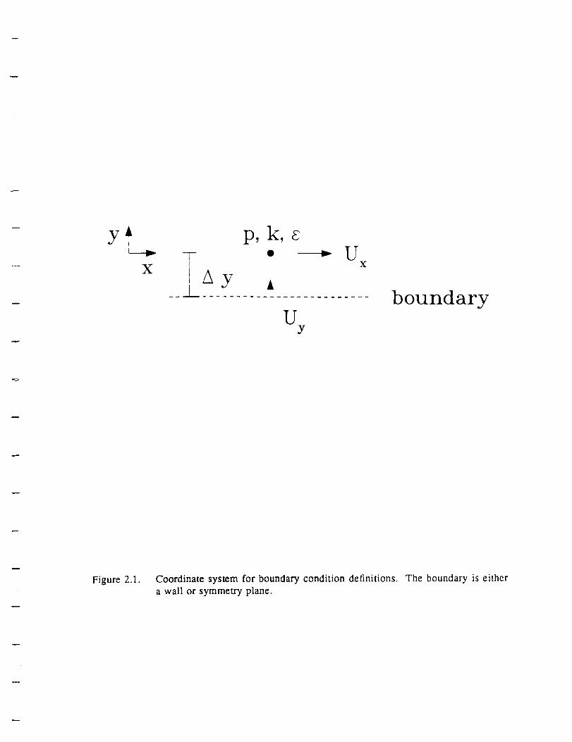
yA Lf
X
p, k,• _ IJ
i X
,_Ay AL .......... P ..............
--- FuY
boundary
Figure 2.1. Coordinate system for boundary condition definitions.
a wall or symmetry plane.
The boundary is either
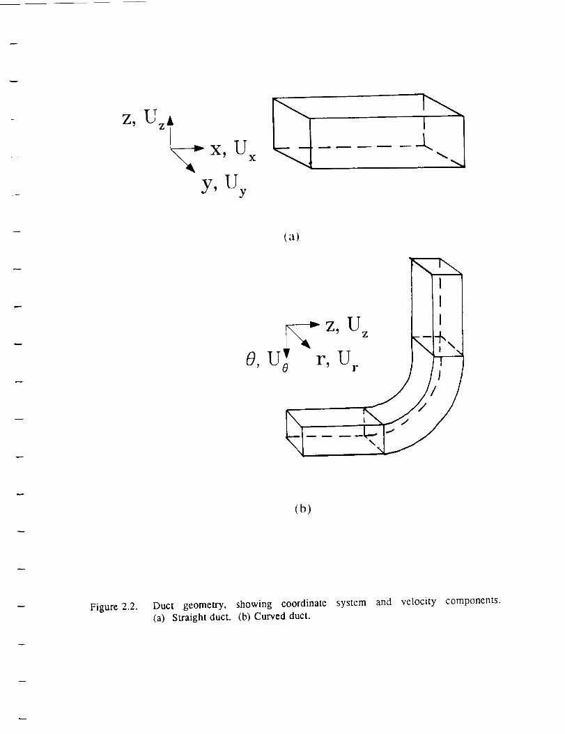
Z, UzA
,'- x, U
y,UY
x
( a )
(b)
Figure 2.2. Duct geometry, showing coordinate system and velocity components.
(a) Straight duct. (b) Curved duct.
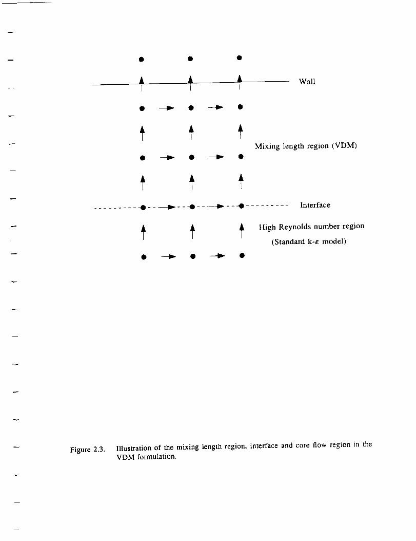
A A A WallI I I
Mixing length region (VDM)
......... -O - - ----_ - - -O - - ----_ - - -O ......... Interface
ttigh Reynolds number region
(Standard k-e model)
Figure 2.3. Illustration of the mixing length region, interface and core flow region in the
VDM formulation.

Ib
I
I
I
I
I
I
I
I
I
I
1
I
I
I
I
I
I
qJ
I
I
I
I
I
I
I
I
I
I
......
I
I
I
I
I
L _
4_
ii ....
XU i X,.
Figure 3.1. Main grid node control volume.
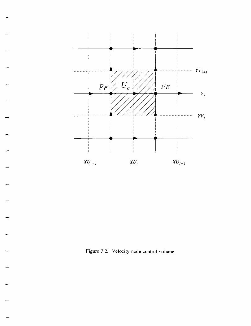
' ' II I
i i II I
I
v ,.
,,',, I..... IL. .............
I .
'' pp_ e b
T ,I
I
I
I)
IIi
Av _
I
I
I
I
I
I
i
I
I
i
I
I
I
I
1
__.... YVj+ 1J
7 -I
I
........ L.. ....
v
gui_ t XU i gui+ 1
Figure 3.2. Velocity node control volume.

i lw i
' NI I
I I
I I
I I
I I
,, ...... ]_'--"','h'7-4_/_ _/,__,_ ............
w _,__, _'_i///,//e/ E"ZJ_ f_K_Y_ ............i S 'I t
! I
I !
I !
I I
I Ilh
S"ill
Figure 3.3. Control volume for intergration of the general ¢_-variable transport equation.
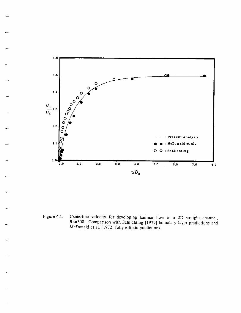
1.0_
0.0
OO
Oo
: Present analysis
@ • : McDonald eta].
0 0 :SchlichtinE
Figure 4.1. Centerline velocity for developing laminar flow in a 2D straight channel,
Re=300. Comparison with Schlichting [1979] boundary layer predictions and
McDonald et al. [1972] fully elliptic predictions.

w
I;o0
- $ d $ 0 o o d o
,e
0.Q
o
Q
m
< _ _ --"r--.m
_ _ '. I' .' I'
-_ < b O o
o o o _ o o o
N
'*-_ ,d _ o.
\D
o.o
A
e'_
,q
c" 0r-,
3. _
o '--
e- e- _
"_. _
_'_ o=.,gq
_= r..) g

2.0
1.8,
1.8
1.4
U_1.2
Ub
o.8-
0.6-
o.4.
o.2-
o.o
_- ¢
o.o 2'.o 4.o 6'.o
: Present Analysis
• Q : Goldstein and Kreid
I
a.o ,b.o LZ.O ,.o le.o l_.o _o.o z_.o ,',.o 28.0 _8.o so.
x/ D},
Figure 4.3. Centerline velocity for developing laminar flow in a square duct, Re=200.
Comparison with data of Goldstein and Kreid [1967].

0.50
: Prement. Analy|i=
Go|dstein and Kreid Predictions0.45
A : x/d = 1.5
× X : x/el = 4 0
0.40. • • : x/d=2o.
I
0.10-
0.00
1.6 1.8 2.0 2.2
Figure 4.4. Velocity profiles for developing laminar flow in a square duct, Re=200.Comparison with data of Goldstein and Kreid [1967].
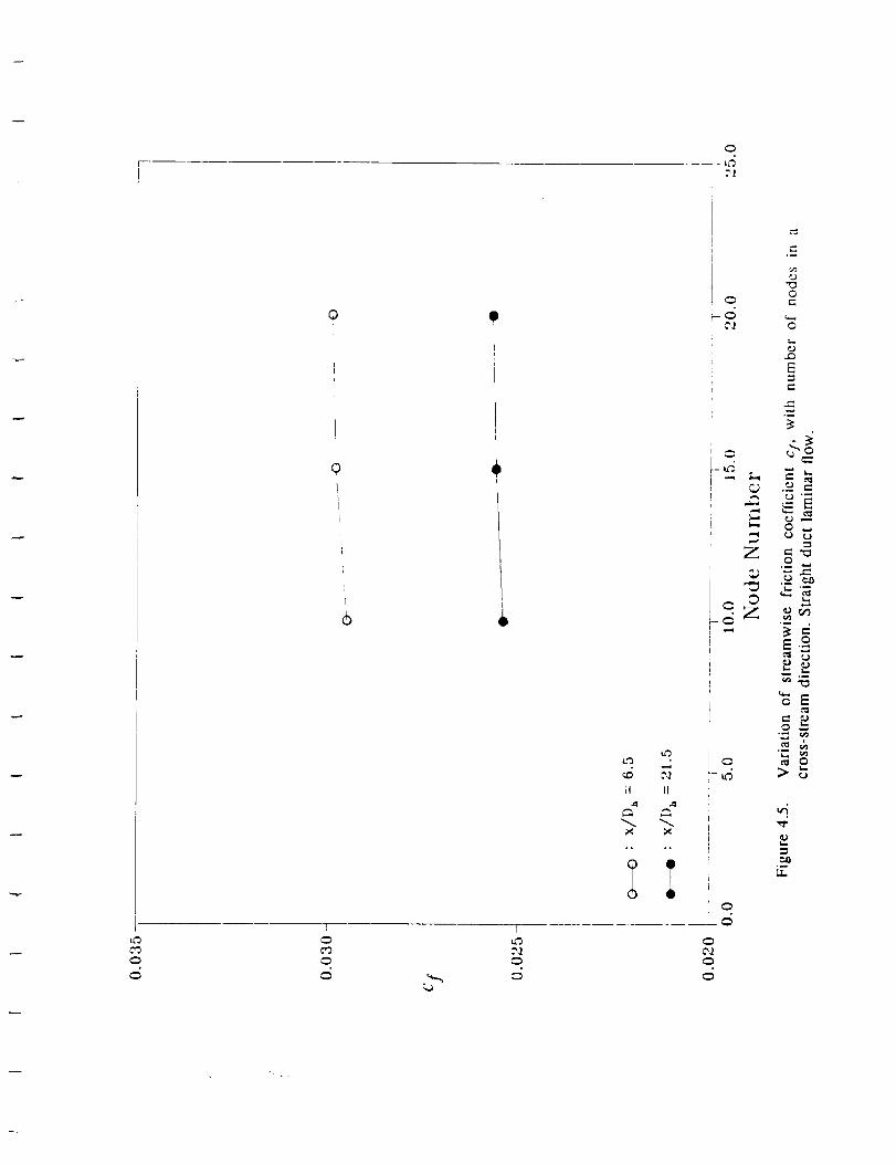
L_
0
0
I
o
L_L_
II II
I.
o
0
J_
jB.
Z
c 0
c_
oc.-
o
ej
E
E.c_
oE
-s
Lfl
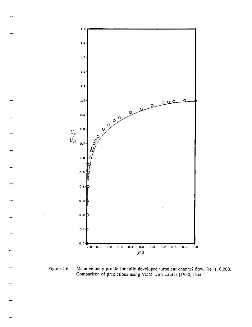
1..5
1.3"
1.2"
1.|"
1.0"
0.9"
0.8
U x
Ut, l0.7
0.8
0._ ¸
0.4-
0.3"
0.2 "
0.1'
o
o2/°
o
0.0_
o.o o.1 d.z 0.3 o'., o.o o.e 0.7 o.e O.o z.o
y/d
Figure 4.6. Mean velocity profile for fully developed turbulent channel flow, Re=110,000.
Comparison of predictions using VDM with Laufer [1950] data.

1.5
1.4 ¸
1.3 -
1,2"
1.1"
_t.0 "
0.8
k---lO0 0.7
oO0
o
00
o
0
0.0 0.1 0.2 0.3 0.4 0.5 0.6 0.7 0.8 0.9 1.0
y/d
Figure 4.7. Turbulent kinetic energy profile for fully developed turbulent channel flow,
Re--ll0,000. Comparison of predictions using VDM with Laufer [1950] data.
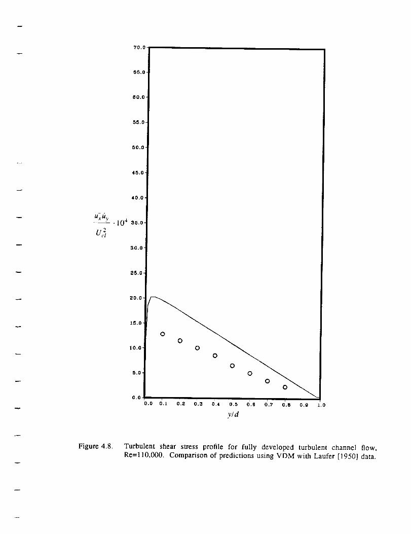
70.0
65.0-
60.0 -
55.0-
60.0-
45.0
40.0
•---lO 4 35.0-
v330.0-
25.0-
20.0 -
15.0-
o
lo.o- 0 0
5.0-
0.0J _ • , i d r
0.0 0.1 0.2 0.3 0.4 0.5 0,6 0.7 0.8 0.9 1.0
v/d
Figure 4.8. Turbulent shear stress profile for fully developed turbulent channel flow,
Re=110,000. Comparison of predictions using VDM with Laufer [1950] data.

U X
Ucl
0.0 0.1 0.2 0.3 0.4 0.5 0.8 0.7 0.8 0.9 1.0
y/d
Figure 4.9. Mean velocity profile for fully developed turbulent channel flow, Rc=110,000.
Comparison of predictions using WFM (standard constants) with Laufer[1950] data.
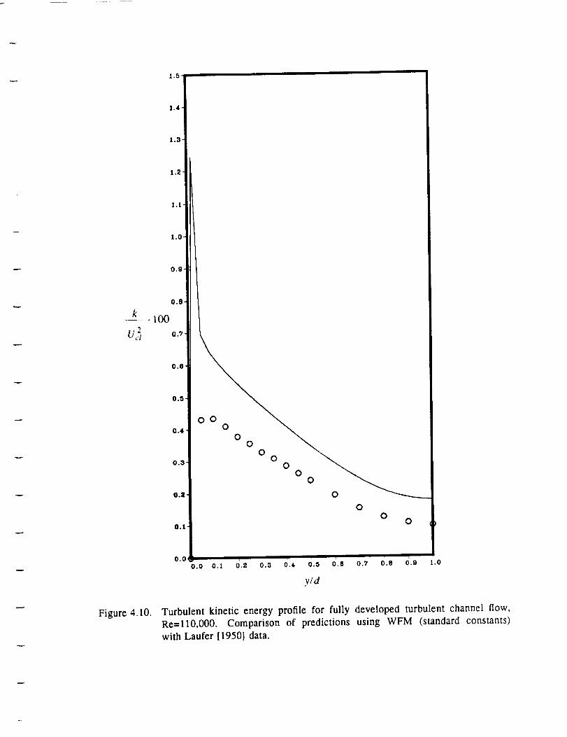
k
ooo
00
0o
00
0
o
y/d
Figure 4.10. Turbulent kinetic energy profile for fully developed turbulent channel flow,Re=ll0,000. Comparison of predictions using WFM (standard constants)
with Laufer [1950] data.
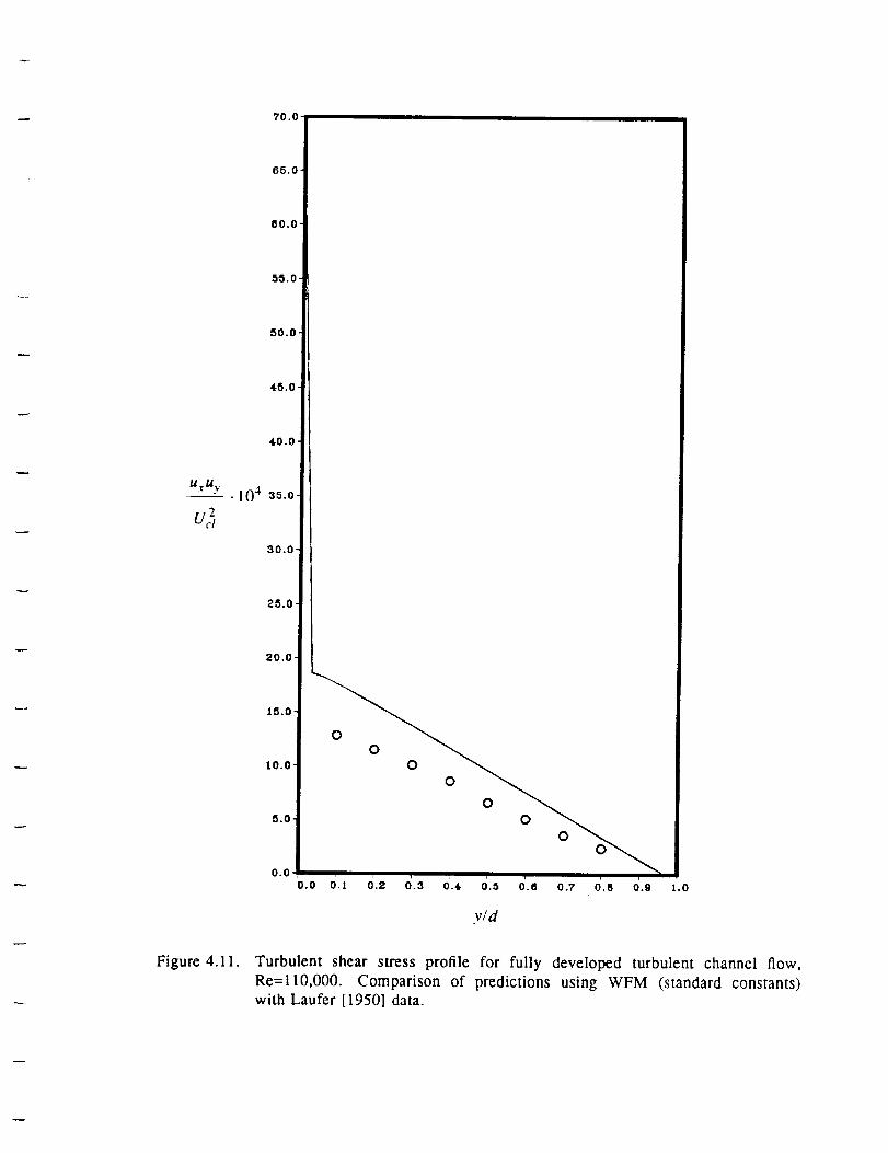
70.0
80.0-
55.0
50.0
45.0'
30.0
25.0
15.0-
LO.O
00
00
0
0
Figure 4.11. Turbulent shear stress profile for fully developed turbulent channel flow,
Re=ll0,000. Comparison of predictions using WFM (standard constants)with Laufer [1950] data.

70.0
65.0
60.0-
55.0-
• 50.0-
4-5.0 -
40.0 -
u'% . tO4 35.0-
30.0.
25.0.
20.0-
15.0-
0.0o.o o.1 0.2 o.3 o., d.5 0.8 o._ 0.. 0._
v/d
1.
Figure 4.12. Turbulent shear stress profile for fully developed turbulent channel flow,
Re=ll0,000. Comparison of predictions using WFM (Laufer's constants)with Laufer [ 19501 data.

1.5
1,3"
1,2"
VDM
U_"
Ub
WFM
Figure 4.13.
0.4 4
0.3"
0.2 "
0.1
0.0o.o 0._ o.2 o.3 0.4 o._ o.6 o._ O.e o.9 z.o
y/d
Mean velocity profile for fully developed turbulent channel flow, Re=110,000.
Comparison of predictions using WFM (standard constants) and VDM with
interface region at y÷ = 10.

1.5
1.4
1.3
1.1-
1,0"
0,_"
0°4 '
WFM
VDM
0,1 o
0°0 o
Figure 4.14. Turbulent kinetic energy profile for fully developed turbulent channel flow,
Re=110,000. Comparison of predictions using WFM (standard constants) and
VDM with interface region at y+ -- 10.

2.4
2.2 -
2.0"
1°8 "
1,6"
1.4 "
1.0"
Ooa "
0.6VDM
0.4
0.2
0.0,o.o o.1 o.2 0.= o., 0.5 O.e o._ o., 0.9 l.o
y/d
Figure 4.15. Energy dissipation profile for fully developed turbulent channel flow,
Re=110,000. Comparison of predictions using WFM (standard constants) and
VDM with interface region at y+ = 10.

140.0-
130.0
VDM
120.0
110.0-
80.0
70.0
WFM
80.0 -
O0.O-
30.0
20.0 -
o.o o.1 &z o.s o., o.s &e 0.7 o.e o.0 z.o
y/d
Figure 4.16. Eddy diffusivity (p,) profile for fully developed turbulent channel flow,
Re=ll0,000. Comparison of predictions using WFM (standard constants) and
VDM with interface region at y+ = 10.
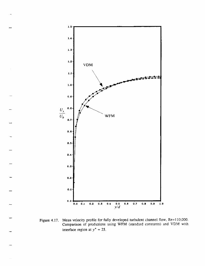
U°_.
Ub
1,4 "
1,3"
1°|"
1.0"
0.g-
o.e
0.7
0.6
0o_ ¸
0,4 "
0°3-
0o2 -
0°1 -
VDM
0.0
yld
Figure 4.17. Mean velocity profile for fully developed turbulent channel flow, Re=110,000.
Comparison of predictions using WFM (standard constants) and VDM with
interface region at y+ - 25.
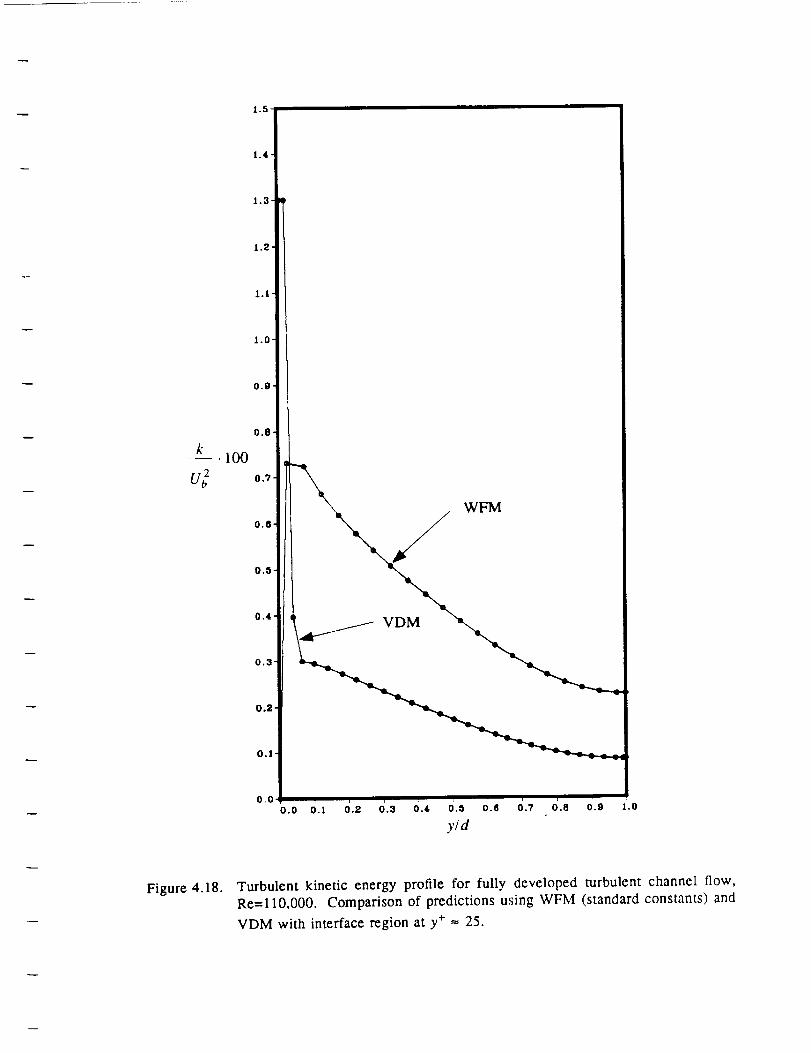
1°| •
VDM
WFM
Figure 4.18. Turbulent kinetic energy profile for fully developed turbulent channel flow,
Re=ll0,000. Comparison of predictions using WFM (standard constants) and
VDM with interface region at y÷ -- 25.
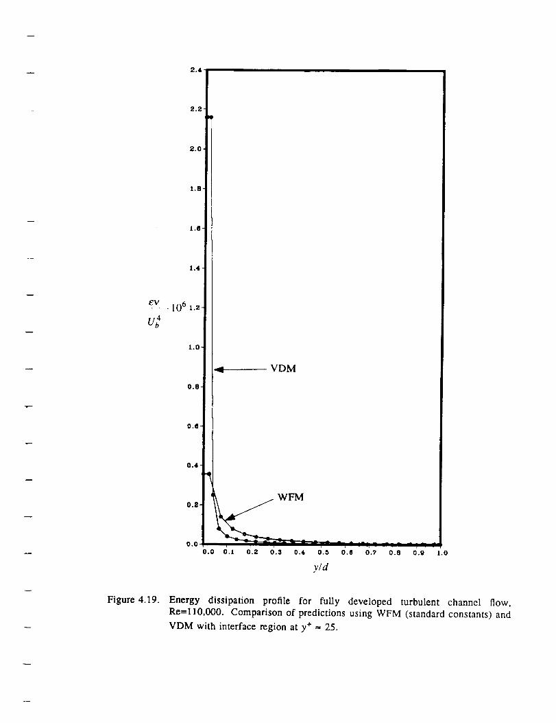
2.4
2.2-
2.0
1.6 -
1.4 "
1.0
Ooe '
0o4 "
---' VDM
0.0 0.1 0.2 0.3 0.4 0.5 0.6 ().7 0.8 0.9 1.0
y/d
Figure 4.19. Energy dissipation profile for fully developed turbulent channel flow,
Re--110,000. Comparison of predictions using WFM (standard constants) and
VDM with interface region at y+ = 25.
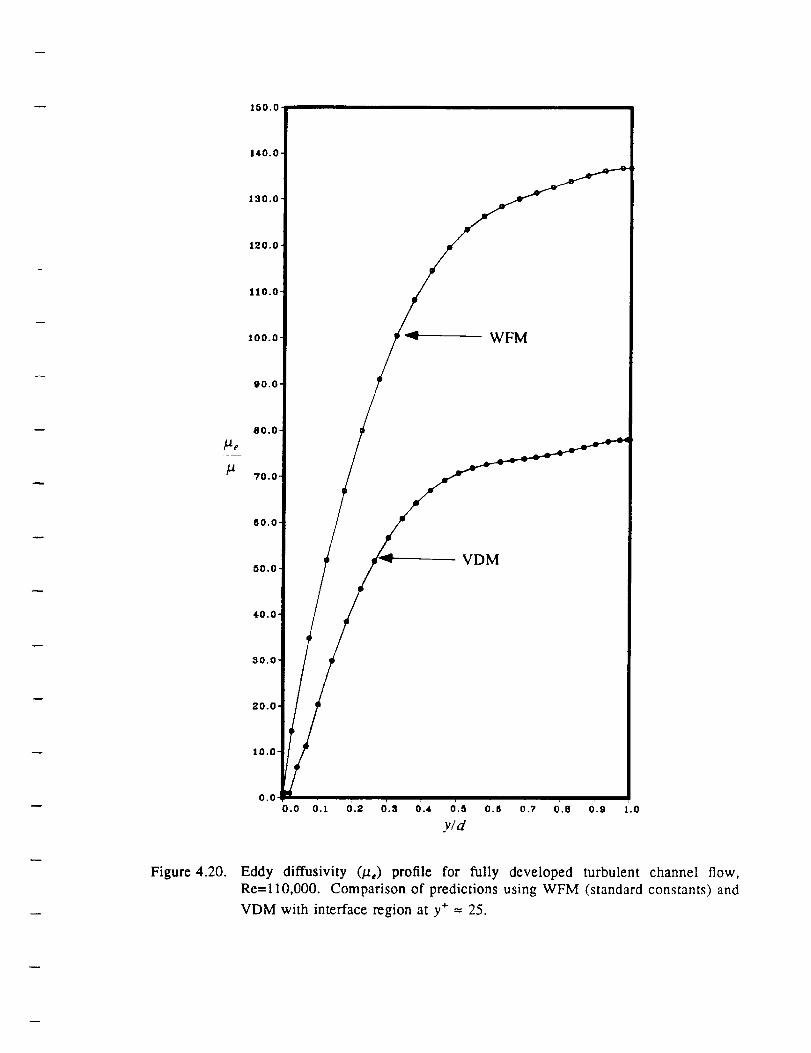
140.0-
130.0
120.0
I10.0
100.0
50.0-
30.0
20.0
10.0-
0.01
0.0
Figure 4.20. Eddy diffusivity (/a,) profile for fully developed turbulent channel flow,Re=ll0,000. Comparison of predictions using WFM (standard constants) and
VDM with interface region at y÷ = 25.
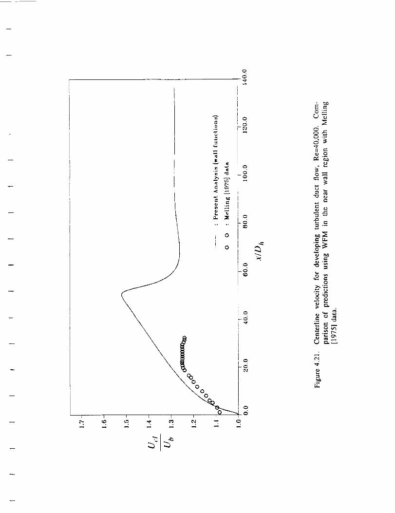
0
=
Wu
=
LO.
0
0
.-w
0
0
,.q
0
CO
0
0
¢D
I-
I --' _ I E I ]
•-w .-w i... _ _,_ _ _'_
o _-_
11¢) 0
_'_
0 ,.-
"_:0
L.
0_°_
8_
_ r _
g _,
t'l

I
'Z,
0
°0
O
II '-'
_'_
0 "
L _
.__ _0
_._ °_
0:_._ ..,-_.
°_ _
6 "_
,4

0
C
0
o
© _.
0
0
0000 00000
IQI I [ r • _ t
= o = ° = = o o o
00
C
0
0
0
c_
C_
Cq
0
CD
c_
c_
II
°_
0
=_= -_
r,.) r..) r-
-i
cL
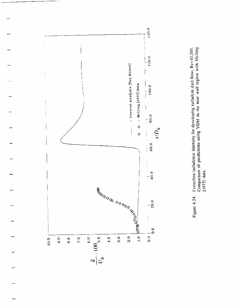
:bOoo °
r_
r_
_ 0
0
\
0 0 O0 0
g___I i
0
Iq
G _
eJ e-,
°_ _
-1
0
._ .,-- ._•-_ _
,4
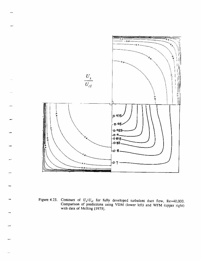
U_
Ucl
Figure 4.25. Contours of U,,/Uct for fully developed turbulent duct flow, Re=40,000.
Comparison of predictions using VDM (lower left) and WFM (upper right)with data of Melling [1975].
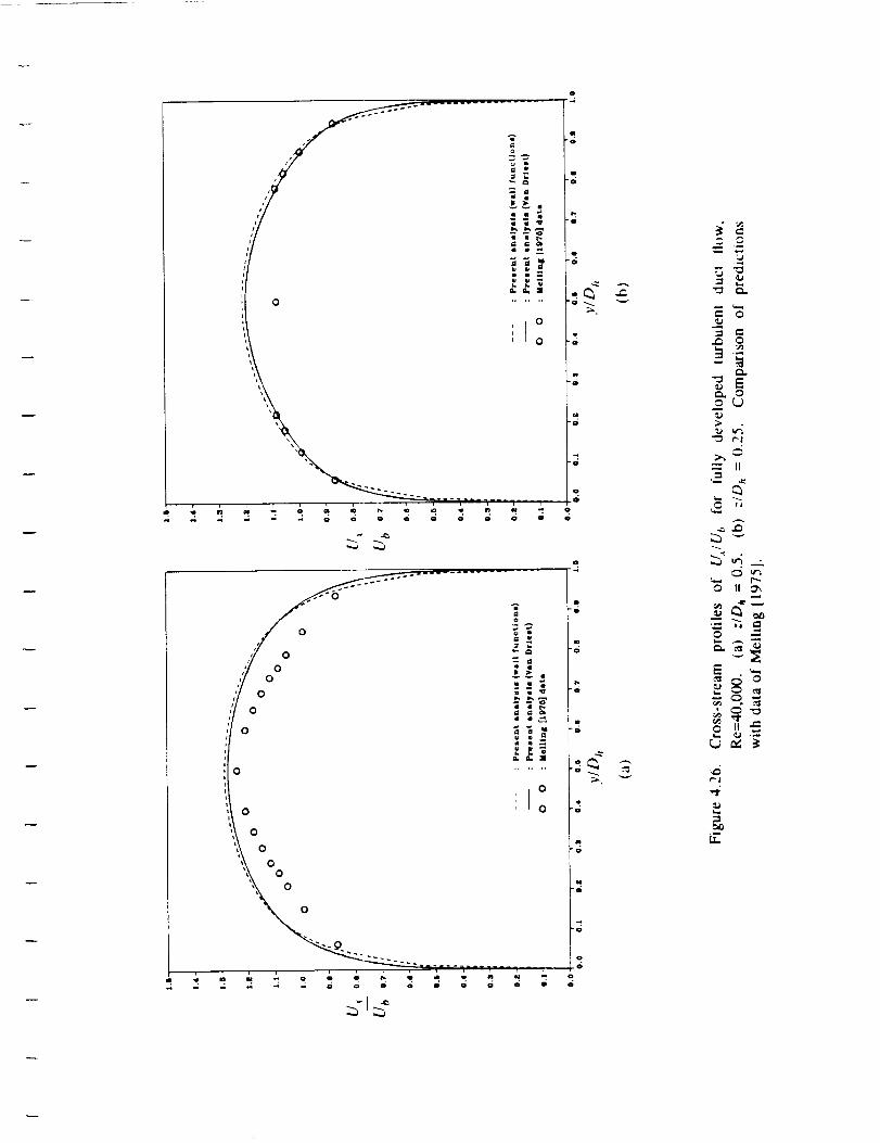
ii_ I °i_ :1o
,o m N o m _. qD Im . _
o
"o
-o
et
o.o
.P,
o
•'- II
Q
t_. r_o II O_
._ g:
.-j.
LX.

I
Figure 4.27. Contours of "_/Uct for fully developed turbulent duct flow, Re=40,000. Com-
parison of predictions using VDM (lower left) and WFM (upper right) with
data of Melling [1975].

0" I
/
/^ o,/
o,_, o
A
_eo
R
a
i1 •
,I °q
' 0
0 _
o/
_ o
ao
• • J-_
, j ot
_ 0
m
i
o
oo
o o
._
K_
z_
_d¢,I
N ..'_

Location of the cross-stream planesin the streamwise direction
I
II
I
I
1.0
0.0 0,_
Cross-stream grid for
WFM formulation
lJ,,
J
i?
h_
0.0
0.0 0.5
Cross-stream grid for
VDM formulation
Figure 5.1. Grid arrangement for curved duct calculations.
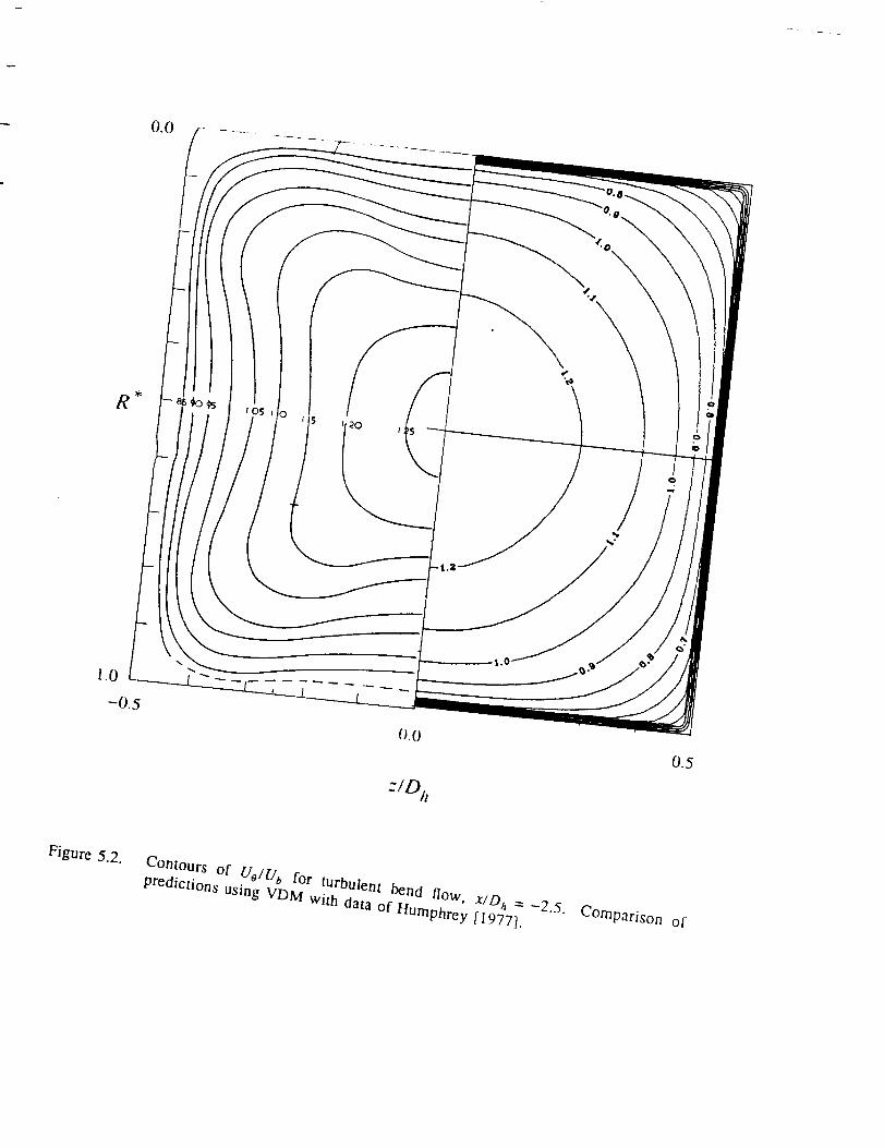
:/D/z
0.5
Figure 5.2.
Contours of Uo/U b for turbulent bend now, x/Dh =-2.5.predictions using VDM with data of Humphrey [1977]. Comparison of

R
f
z/D h
Figure 5.3. Contours of UelUb for turbulent bend flow, x/Dh =-2.5.predictions using WFM with data of Humphrey [1977].
Comparison of

0
0.7 "a'_• _E
0,,'/_/ ,--
,:_ : .: :_
_,\°, ' , o )
0"
0', i0 o
° 0 _
0 "_
.'_ ._. _"
0
toio,\o
i°
0
r--i
r-
e-
t....o
0
e'.
c
_.o II
_ °
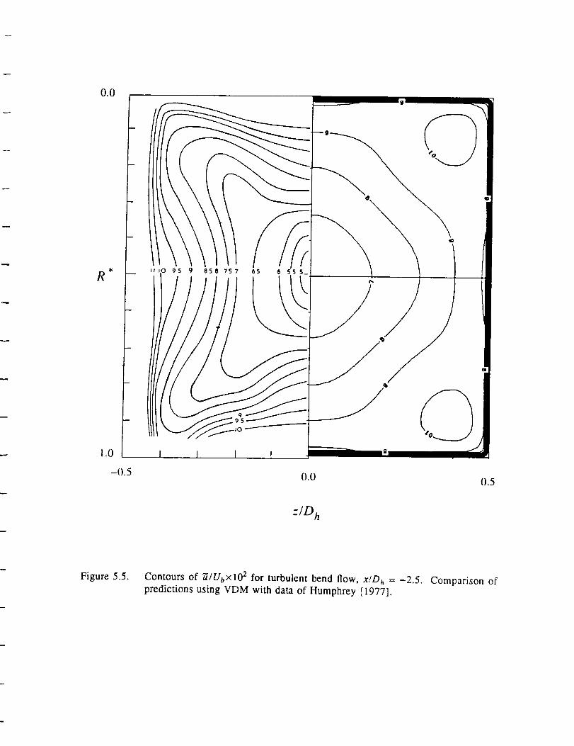
0.0
:¢R
rI
I 1 I
0.0
:/D h
0.5
Figure 5.5. Contours of _/Ub×102 for turbulent bend flow, x/Dh = -2.5.
predictions using VDM with data of Humphrey [1977].
Comparison of
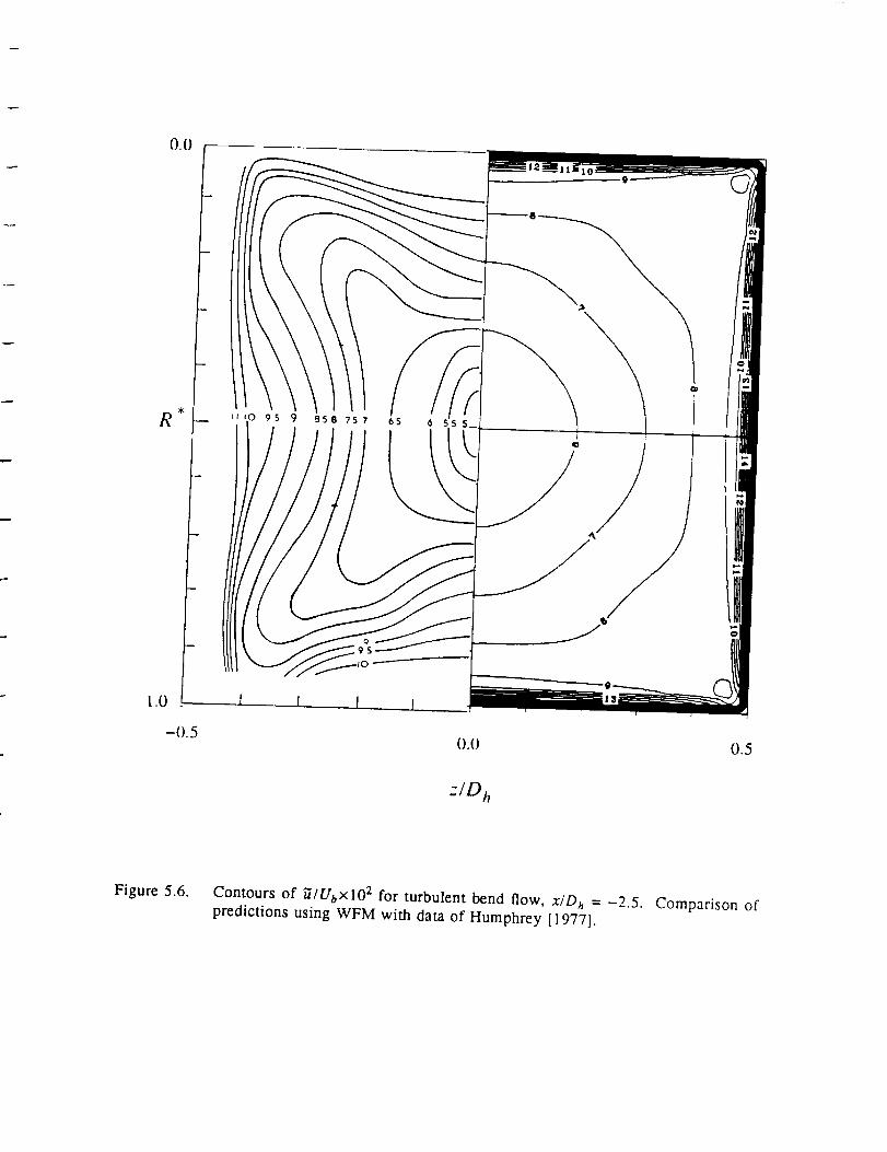
°° I
-0.5
7./D h
Figure 5.6.Contours of _/Ubxl02 for turbulent bend flow, x/D h = -2.5. Comparison ofpredictions using WFM with data of Humphrey [1977].
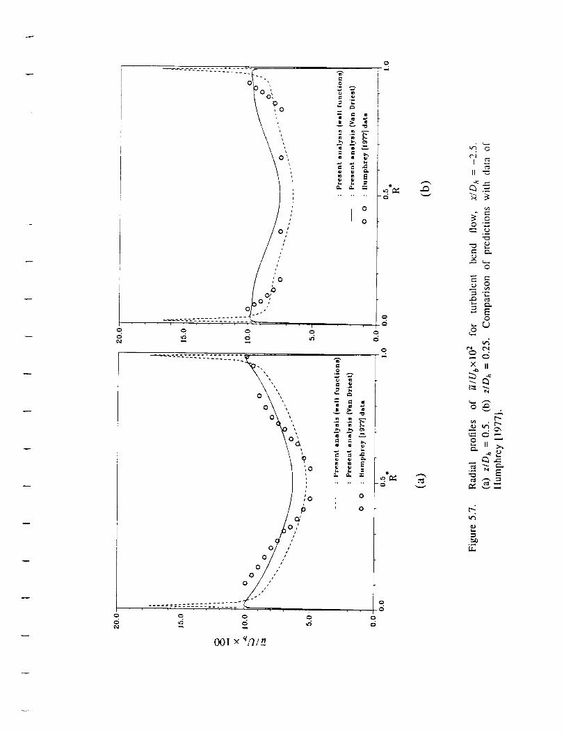
CD
0 C_I
CD
0 \ ',,
0 _ _
J
P
¢
/
i
0
O
' -1 ' '---'--"--- , "gl
.,.,,0
2 :
_ _-,
_.. ea
,I °' O
O
_ ';
.°
:1
"N'
.°
o
O
O
O
O
-O
O
O
("4
e- e'_
O
e_
O
o
X
o
2
rz
C,I
II
N
II >_
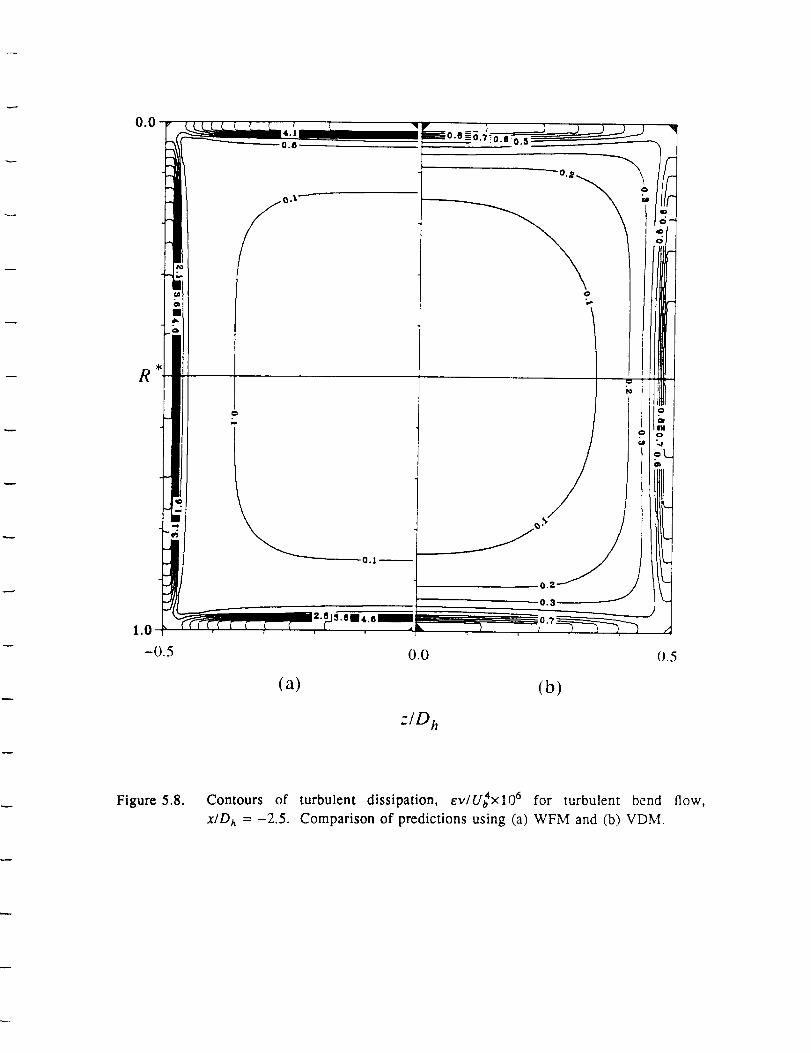
R
(a) (b)
z/D h
Figure 5.8. Contours of turbulent dissipation, _,v/U4×lO 6 for turbulent bend flow,
x/D h = -2.5. Comparison of predictions using (a) WFM and (b) VDM.
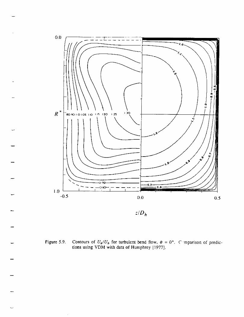
R I 3OI 25
II
0.0 0.5
z/D h
Figure 5.9. Contours of Uo/Ub for turbulent bend flow, 0 = 0 °. C "mparison of predic-
tions using VDM with data of Humphrey [1977].

I 30
Figure 5.10. Contours of Ue/Ub for turbulent bend flow, 0 = 0 °. Comparison of predic-
tions using WFM with data of Humphrey [1977].
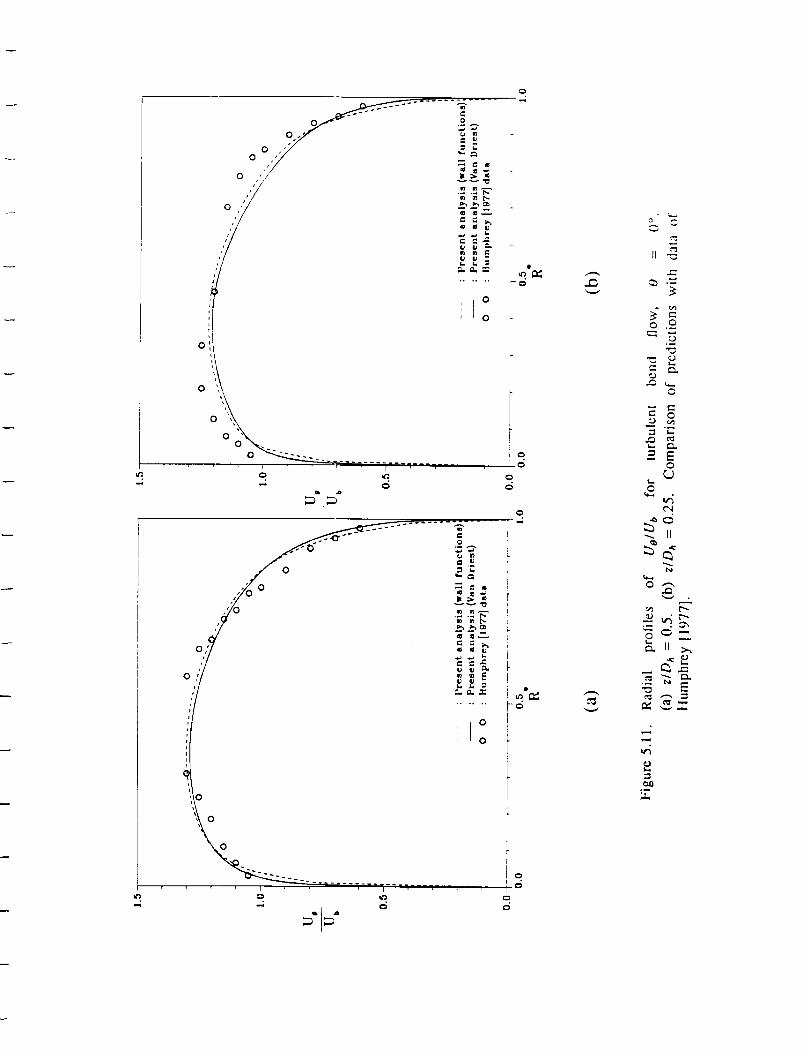
I
v ,/ G G
o,y _
,. o...
0
't
o G
_'_
_g
o_ .
o
_.,-_

0.0
R
1.0 I 1 I l
-0.5 0.0 0.5
z/D h
Figure 5.12. Contours of "ff/Ub×lO 2 for turbulent bend flow, 0 = 0 °. Comparison of pred-
ictions using VDM with data of Humphrey [1977].
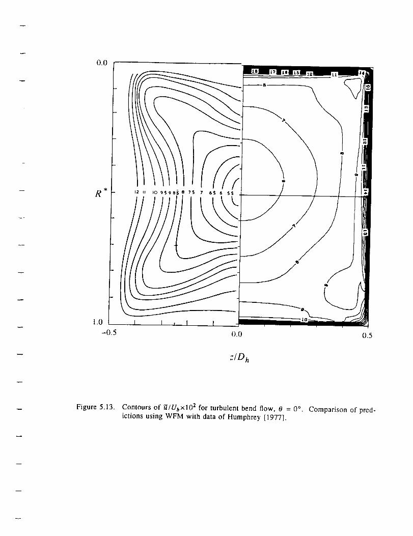
R
z/D h
Figure 5.13. Contours of _/Ubxl0 z for turbulent bend flow, 0 = 0 °. Comparison of pred-
ictions using WFM with data of Humphrey [1977].

0
o_
'"iL
,i
E
/
0
0
0
Io
0 '_
0 _'_
_ '"000_0,._ _ _ _ _ *,_
0_ e- _
o' ® ® _'la la
I.. I= .a
,I °
°i : °
o_/':
001 x _/_
L
I
I°! =
..C:q_ --.
0 0
0
r"
x
0
0
°_
0
E0
II
c_
.
<u
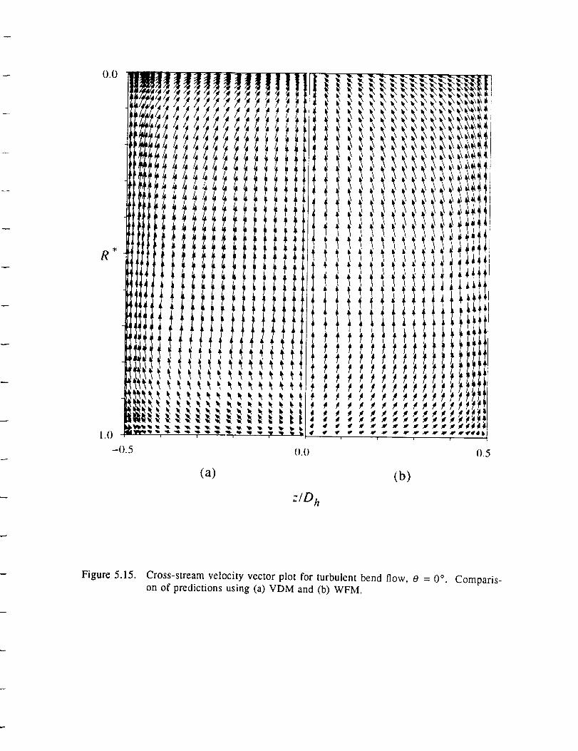
R
i •
i •
i •
l •
(a) (b)
ztD h
Figure 5.15. Cross-stream velocity vector plot for turbulent bend flow, 0 = 0 °. Comparis-on of predictions using (a) VDM and (b) WFM.

().0 O.5
(a) (b)z/D h
Figure 5.16. Contours of turbulent dissipation, tzv/U_×lO 6 for turbulent bend flow, 0 = 0 °.
Comparison of predictions using (a) WFM and (b) VDM.
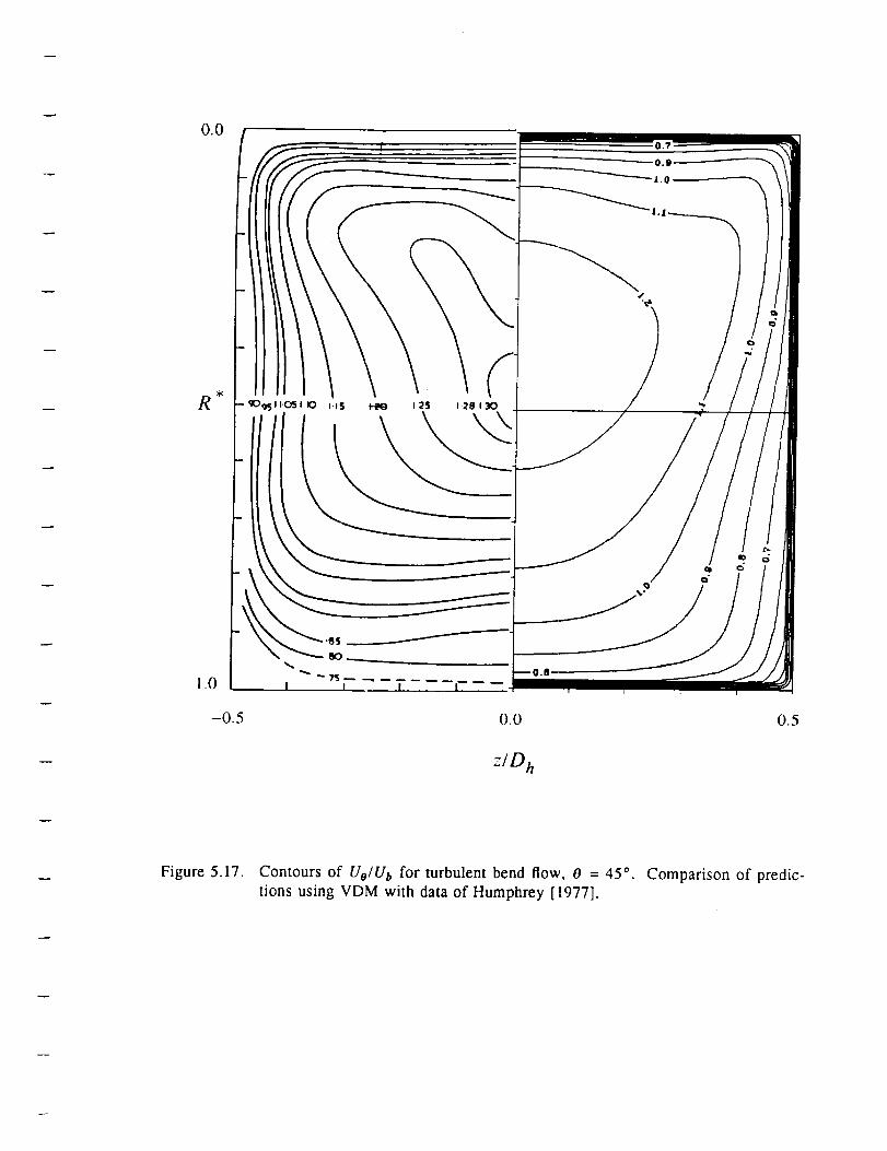
R
I I
-0.5 0.0 0.5
z/D h
Figure 5.17. Contours of Uo/U b for turbulent bend flow, 0 = 45 °. Comparison of predic-
tions using VDM with data of Humphrey [1977].

0.0
R
z/D h
Figure 5.18. Contours of Uo/U b for turbulent bend flow, 0 = 45 °.
tions using WFM with data of Humphrey [1977].Comparison of predic-
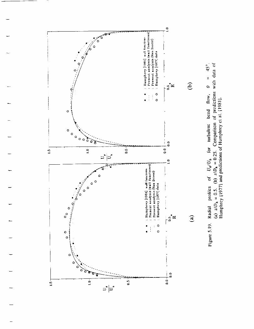
SIKi/t
,.o' ,,"
• ,
0
0
0
0
0
0
0
...... ,n- - - ..... ,
I
.0";
.... _ .,,_ .,_.
sll 16 _ .,,a
0 .i.-.
(3
: 1°0
------:-- ,
C}
I
C,
II
¢J
_ o _
L.0 O
N
_:_ II _,,
o_
v_
L_
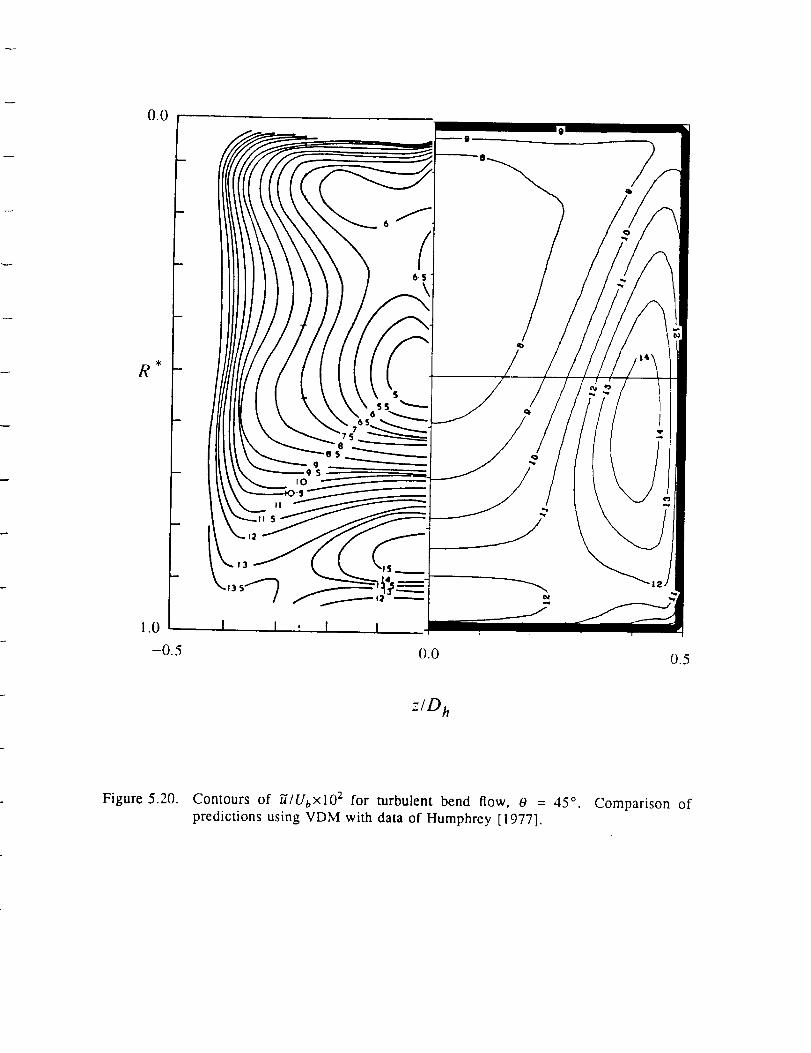
R
65
I!
$
1.0 I : I !
-0.5 0.0 0.5
z/D h
Figure 5.20. Contours of "_/Us×IO 2 for turbulent bend flow, 0 = 45 °. Comparison ofpredictions using VDM with data of Humphrey [1977].

0.0
_g
R
6S
S
SS6
- 7 6
'S
q'SS_
1.0 I I , 1
-0.5 0.0 0.5
:/D h
Figure 5.21. Contours of g/Ubxl02 for turbulent bend flow, 0 = 45 ° . Comparison of
predictions using WFM with data of Humphrey [1977].
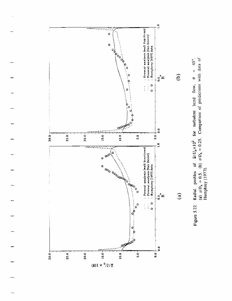
o
I ,,tf
0
o
0
0
%',,%
_0
_ 0
'!!
iJ
,L °' 0
o
o
t
o
°°o Ooo_\ ', $_
e., el e,
_!o ° :t °o,_
o_
0 0 0 0 0
OOTx ¢f2/_.n
o.0
c_
r,,
o 0ug
II "_e-,
o
o
,.-s ¢._
,-s e-_
"" E
Ol
,
L_
._

R
(a) (b)
z/D h
Figure 5.23. Cross-stream velocity vector plot for turbulent bend flow, 0 = 45 °. Com-
parison of predictions using (a) VDM and (b) WFM.
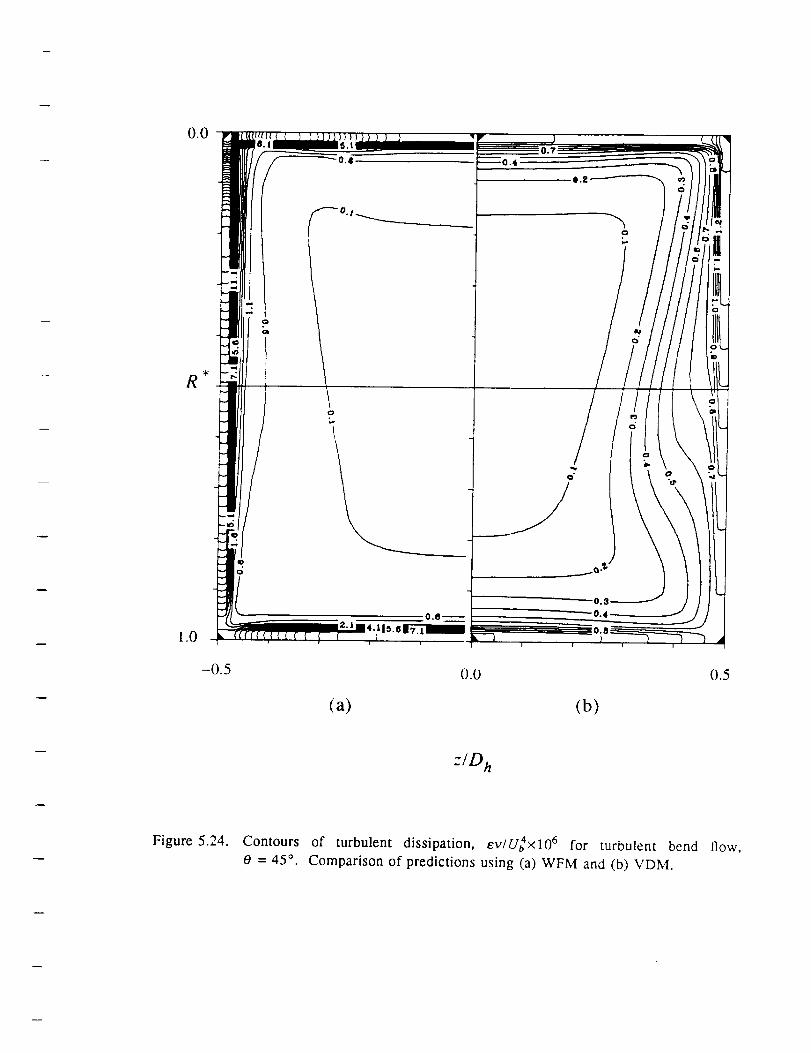
R
-0.5 0.0 O.5
(a) (b)
z/D h
Figure5.24. Contours of turbulent dissipation, ev/U4×lO 6 for turbulent bend flow,
0 = 45 °. Comparison of predictions using (a) WFM and (b) VDM.
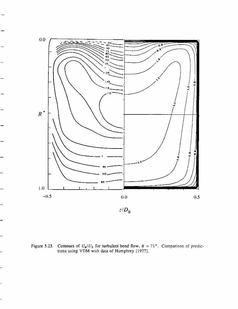
0.0
R
1.0
-0.5
I I , I
0.0 O.5
:/D h
Figure 5.25. Contours of Ue/Ub for turbulent bend flow, 0 = 71 °. Comparison of predic-tions using VDM with data of Humphrey [1977].
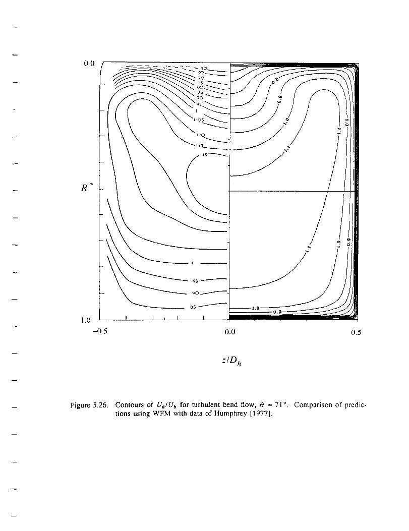
R
f13
95
I I , I
z/D h
Figure 5.26. Contours of UelUb for turbulent bend flow, 0 = 71 ° Comparison of predic-tions using WFM with data of Humphrey [1977].

p
i
ilo
0 _
o '.-_
o _
,]o
' t
4
0000
---.-- -.... - E_0 _ 0
0
0
i_ *_ _-0
i
/ 0 I
04
A
e,0
_ 0
', i I_ _ 0
0 0 "'.0 _
0
L
tO
0
0
o C
IIe,-,
°_
e_
,N
o
Eo
II
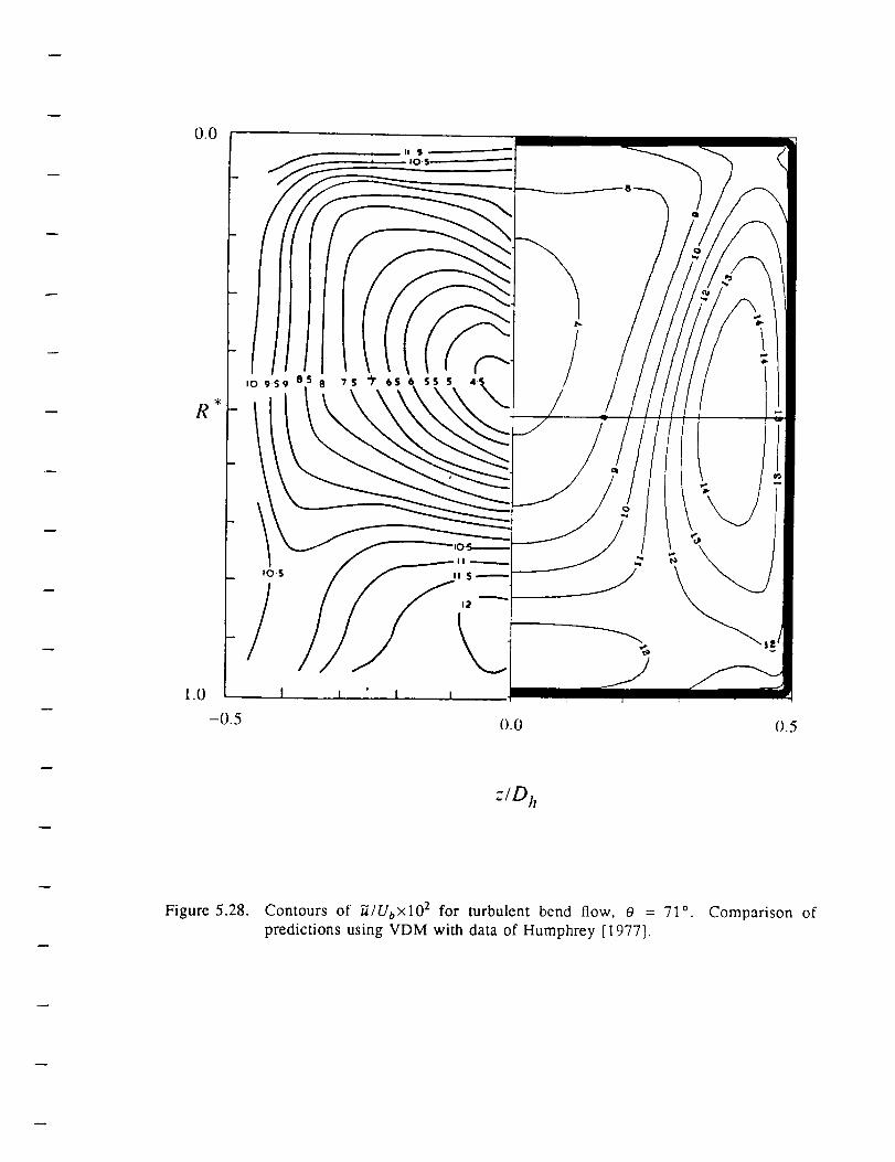
0.0
e¢
R
/I0 959 8 8 7S "_ 6S 6 SS S
/ 1,,
1.0 t L ' t
-0.5
z/D h
Figure 5.28. Contours of "ff/Ub×lO z for turbulent bend flow, 0 = 71 °.
predictions using VDM with data of Humphrey [1977].Comparison of

zlD
Figure 5.29. Contours of "_/UbxIO 2 for turbulent bend flow, 0 = 71 ° Comparison of
predictions using WFM with data of Humphrey [1977].

' ' I
o
....... =_::l:::iiilii:--_,
i
0i
0 _
O'
OilQ
_'0
q
ooo ,"
0 0 _ 0
0
"e i"= I
{_ L
.___._ J
...... _ 0
, I 0 ,
I
F
o
rrl,l,,,
_50 _ ," ' -- = =
', :e_°o ', [ [ F
°o ',, ._ -__
i
o
i i 0
d_
oo ,
o ,/
/0 ,
0 /
° _:0 ,
OOl x q/l/n
0
o 0
o o'.7.
N c
x ,
N
t_
°_

(a)0.0
(b)
0.5
Figure 5.31.
Cross-stream velocity vector plot for turbulent bend flow, 0 = 71 °parison o._ predictions using (a) VDM and (b) WFM. Corn-

0.0
R
(a) (b)
zlD h
Figure 5.32. Contours of turbulent dissipation, evlU4×lO 6 for turbulent bend
0 = 71 °. Comparison of predictions using (a) WFM and (b) VDM.
flow,
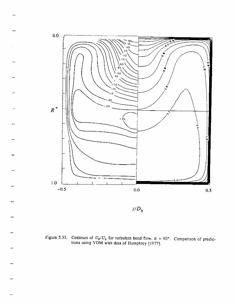
R
I I I
z/D h
Figure 5.33. Contours of Uo/U b for turbulent bend flow, 0 = 90 °.
tions using VDM with data of Humphrey [1977].Comparison of predic-
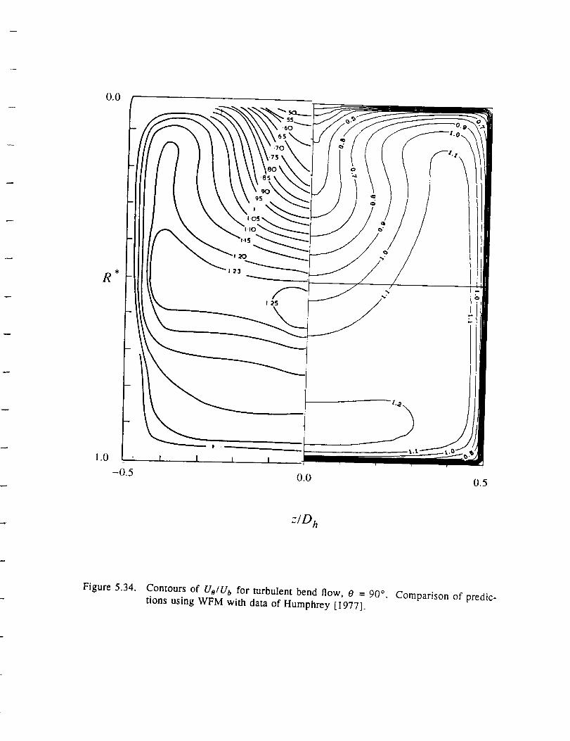
0.0
R
1.0 I t
-0.5 0.0 0.5
z/D h
Figure 5.34. Contours of Ue/Ub for turbulent bend flow, 0 = 90 °. Comparison of predic-tions using WFM with data of Humphrey [1977].
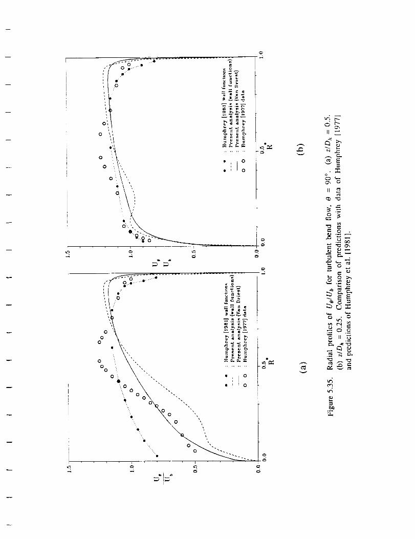
L
0
00
0
o
\
o
0
II '--"
a , .b-"
._'_
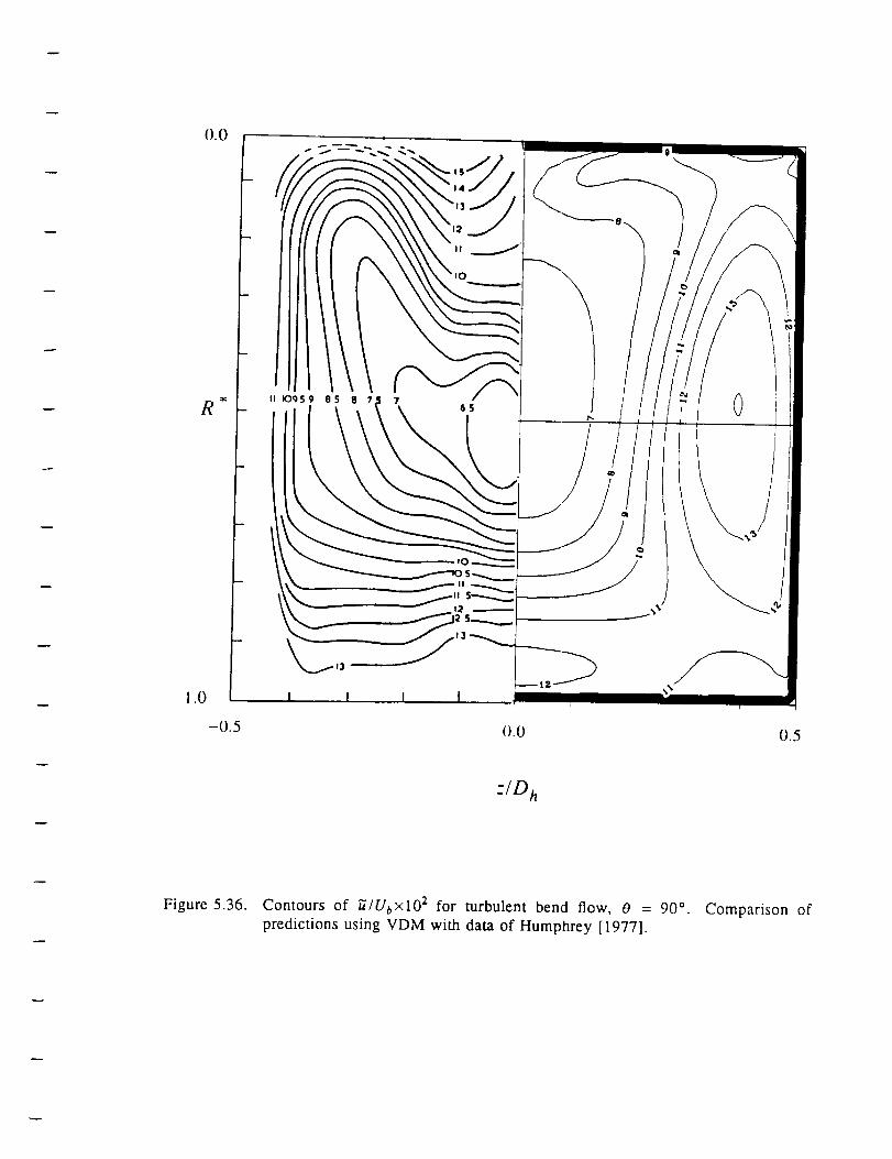
0.0
R
().0 0.5
-/D h
Figure 5.36. Contours of _/Ub×lO 2 for turbulent bend flow, 0 = 90 °. Comparison ofpredictions using VDM with data of Humphrey [1977].
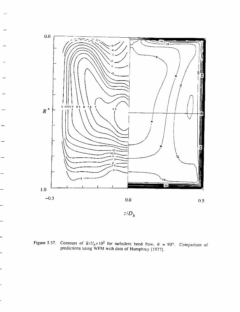
II I0959 05 fl 7 765
I0
/
I I
0.0 0.5
-ID h
Figure 5.37. Contours of _/Ub×102 for turbulent bend flow, O = 90 °. Comparison ofpredictions using WFM with data of Humphrey [1977].

i Oo,,o
L
,,'0
L
i
t
0
!o
0 _D t-_ O 0
"W
o
._._.
", I 00
0
0
-- °OOoo_,* "_°Oo_x ',, .-..-,._.
-OoXx ,., _,_
o
0o
o° ,0
0
o o _ ,,
..... _,'Z-. i 0
00! x q_/_
G__'-_
o o
G
o
II
I,,i
0 _..__''_ .
_1'_
"_'o "_ _
06
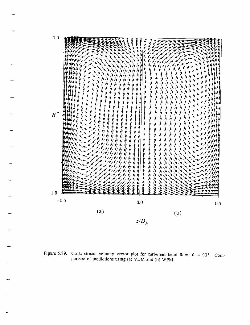
R
0.0
(a) (b)
z/D h
0.5
Figure 5.39. Cross-stream velocity vector plot for turbulent bend flow, 0
parison of predictions using (a) VDM and (b) WFM.= 90 °. Com-
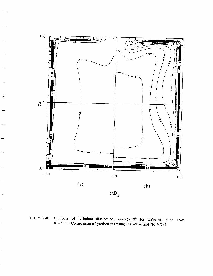
R
(a)
z/D h
(b)
05
Figure 5.40. Contours of turbulent dissipation, e.v/U4×lO 6 for turbulent bend flow,
0 = 90 °. Comparison of predictions using (a) WFM and (b) VDM.

in-
Jn
, um,11r E
%
iJ,' s
"II"E _G G
i._- -, -mm" _0
0
/o
_°°"E
N
_ T j i j i
I I I
.... °, °°
I'OE '
o
i I
I I
_E
_._ _ •..,,_
--E
_s
_° !___
N H----
I

.... oo o.
Q •i
[] •
I j
I
I , l I
• o .
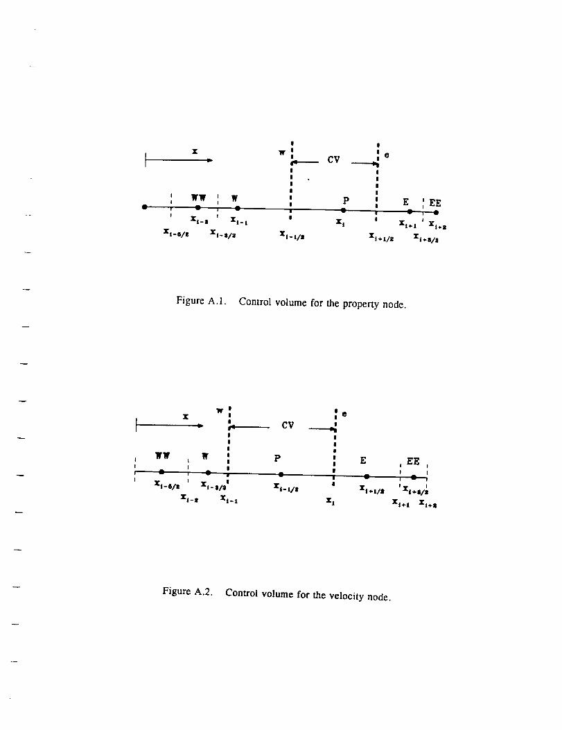
|
X W !|
||||
i WW _ W |! t |
|! !XI- 8 ZI- t
XS_e/s X j_ a/Z XS- t/S
|
I e|
CV _|I||
p ||
X!
Xl÷l/2
'EEE ,
IXl_-I XI+ t
Xs.a/a
Figure A.1. Control volume for the property node.
"ff'| |e|X |
' CV '
o |o |
o o
WW , W ' P ' E| |
dlt
xs_o/s ' xl_,/s' xs_t/s xa+t/_
TI- | Xl_t I 1
EE! I! I
--l÷l/I
X14. t 'rl_. a
Figure A.2. Control volume for the velocity node.
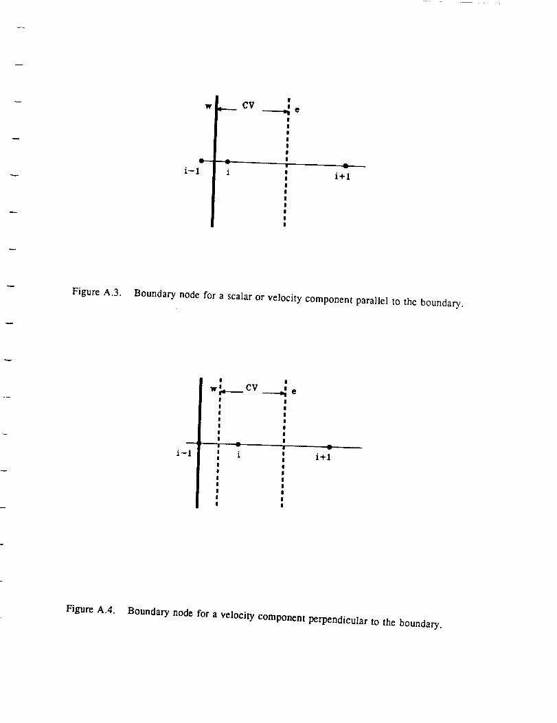
W
i-I
ICV
I e
III
III
I
I
I
I
I
I
I
I
Figure A.3. Boundary node for a scalar or velocity component parallel to the boundary.
i-I
"k ---cv ----4 eI I
I l
I I
I l
I I
I I
l I
i i o
! |
| I! || |o o! |
| i
i+l
Figure A.4. Boundary node for a velocity component perpendicular to the boundary.
Top Related