


Languages
Pages
Legal


UNIVERSITY OF CANTERBURY, WORLEYPARSONS, CONTACT ENERGY
Investigating Retrofitting an Existing
Geothermal Power Plant with a Biomass
Gasifier for Additional Power Generation
A Thesis Submitted in Fulfilment of the Requirements for the
Degree of Master of Engineering in Chemical and Process
Engineering
Steven Chester
9/10/2016

iii
Abstract
Hybridization of geothermal and biomass resources for power generation is a potential step in the
increased commercial utilization of biomass gasifiers in New Zealand. There is generally an
increase in the power generation efficiency by hybridizing two power generation technologies.
Hybrid power generation also reduces the capital costs for power plants, due to shared equipment.
The Taupo Volcanic Zone is home to a large geothermal reservoir, is proximate to the largest area
for commercial forestry in New Zealand, and is therefore a promising location for hybridizing
geothermal and biomass resources. The Wairakei Power Plant has been used to generate power for
over 50 years, but declining reservoir enthalpy and the preferential use of geothermal steam at
other geothermal power plants causes there to be unused power generation capacity.
This study examines the potential for integration of biomass gasification as an additional fuel
source in the Wairakei Power Plant so as to increase power generation. Possible approaches to
integrating syngas firing into the steam system were investigated and the derived hybrid
configurations modelled using the heat and material balance software UniSim to estimate the
additional power generation possible. Experimental work was limited to measurements on steam
condensate in the existing geothermal systems so as to establish steam purity and required clean-
up approaches to utilize steam condensate as a source of boiler feed water. This study addresses
some of the practical problems related to silica carryover and plant integration so to allow the
utilization of biomass synthesis gas to directly heat geothermal steam.
Four hybrid configurations were investigated in order to generate additional power by integrating
a biomass gasifier and syngas fired heating to the Wairakei Geothermal System:
Superheating of geothermal steam for more efficient power generation
Syngas fired heating used to boil condensate available on site for additional steam
generation
Boiling separated geothermal water immediately after the first separation stage
Heating of separated geothermal water available at Wairakei to increase power generation
at an existing binary power plant
The performance of the dual fluidized bed gasifier was seen to achieve cold gas efficiencies as
high as 84% based on the lower heating value of the landing residue feed and the generated syngas.
However, this does not include the thermal input of steam used as the gasification agent, as
geothermal steam generated on the Wairakei Geothermal Field was used to satisfy this steam
requirement. Flue gas from the biomass gasifier and the combustion of syngas on site was used as
the drying agent to dry the wet wood chips prior to these wood chips being introduced to the
gasifier.
It was found that the geothermal steam supply to Wairakei greatly impacts the power generation
that is possible the hybrid configurations. Three scenarios for the potential steam supply conditions
were created in order to represent the changes in the additional hybrid power generation that is
expected to occur with changing reservoir enthalpy:
iv
Scenario 1: Steam supply consistent with that for January 2015 – July 2016. Sporadic
bypassing of turbines by intermediate pressure steam occurs, all steam turbines at Wairakei
are fully loaded.
Scenario 2: Reduced steam supply to Wairakei. No steam bypassing occurs, all steam
turbines at Wairakei are fully loaded.
Scenario 3: Further reduced steam supply to Wairakei. No steam bypassing occurs, but not
all steam turbines are fully loaded. Additional generated steam may be used in partially
loaded steam turbines to increase power generation.
Capital cost estimation and an economic evaluation was performed for the proposed hybrid plants
in order to quantify the financial implications of implementing the hybrid configurations for each
of the steam flow scenarios investigated.
In order to modify the 30 MWe mixed pressure geothermal steam turbines to utilize superheated
steam, it was found that there would be an estimated 2.6 MWe decrease in the power generation
of the turbines when fully loaded. However, as the modified turbines will use less steam compared
to the unmodified turbines, there is a net increase in power generation possible, due to the power
generation that may be performed using the saved geothermal steam. This configuration was seen
to be the most efficient in Scenario 3, where an average additional power generation of 11.9 MWe
is possible from a 15 t/h input of wet landing residues. This resulted in a fuel to electricity
efficiency of 29.7% based on the lower heating value of the landing residues. The project was,
however, expected to lose $27 million over a 30 year hybrid plant life, and required an estimated
capital investment of $48 million.
Water testing was performed on several sources of water available on the Wairakei Geothermal
System, in order to evaluate suitability as boiler feed water. It was found that the most appropriate
source of water was condensate from the Poihipi Rd Power Plant, which has an estimated average
of 54 t/h of condensate available for use. A water cleaning process was then designed based on the
contaminants present in the water, in order to ensure safe and reliable operation of the boiler. The
process modelling revealed that this configuration generated electricity most efficiently in the
conditions of Scenario 3, with an average of 6.2 MWe additional power being generated from a 15
t/h input of wet landing residues. The resulting fuel-electricity was calculated at 14.8% based on
the lower heating value of the forest residues. There was a projected loss of $32 million from the
implementation of this project over a 30 year hybrid plant life, requiring a $9.6 million investment.
It was found that boiling separated geothermal water after the first separation stage resulted in a
decrease in the metals being discharged into the Waikato River due to an increased proportion of
the metals being reinjected into the geothermal reservoir. It was found that power could be
generated most efficiently in the conditions of Scenario 3, using the additional steam created from
boiling the separated geothermal water. An estimated 6.8 MWe of additional electricity could be
generated using an input of 15 t/h of wet landing residues, resulting in a fuel to electricity efficiency
of 16.2% based on the lower heating value of the landing residues. The project was expected to
lose $27 million for a 30 year plant life, and required a capital investment of $8.3 million.
The Wairakei Binary Plant is designed to generate an average of 15 MWe, however an average
generation of approximately 13 MWe has been observed for the plant, this is attributed to the
flowrate of separated geothermal water being lower than the plant was designed for. In order to
supplement the separated geothermal water flow to the Wairakei Binary Plant, the additional

v
geothermal water was expected to require heating in order to avoid increasing silica scaling in the
Binary Plant. The heating of additional separated geothermal water for use in the Wairakei Binary
Plant was seen to have the highest efficiency in Scenario 1. An increase of 1.4 MWe was expected
using a 3.4 t/h average wet wood input, resulting in a fuel to electricity efficiency of 15.5%, based
on the lower heating value of the wet landing residues. This project was expected to lose $17
million over the 30 year life of the hybrid plant, and require a capital investment of $7.8 million.
The poor economics associated with implementing any of the hybrid configurations are attributed
both to the design constraints of retrofitting the hybrid configurations, and the relatively high cost
of the landing residues. It was initially thought that the close proximity and availability of forestry
landing residues would result in viable options for boosting geothermal power generation using
syngas fired heating. However, due to the inefficiencies associated with retrofitting the hybrid
configurations to an existing geothermal plant, and the relatively low sale price of power; the
delivered cost of the forest residues was seen to exceed the value of the additional power generation
in most cases. It is therefore recommended that the integration of a gasifier into a new geothermal
plant from the design stage, and alternative, cheaper, feedstocks for gasification be investigated. It
is also believed that the generation and sale of liquid biofuels using geothermal steam as an input
to a gasifier may prove to be profitable.

vi
Acknowledgements
I would first like to acknowledge Callaghan Innovation NZ for its funding support of this project.
Thanks to my supervisors, Chris Williamson, George Hooper, and Mike Dunstall, for their help
and advice throughout the course of this project, without them, this project never would have
happened.
The Staff and Management at Contact Energy’s Wairakei Plant, where I spent several months
researching, were beyond helpful, and very welcoming. The commercial perspective was
invaluable in ensuring this project took practical considerations for retrofitting the Wairakei Plant
with biomass gasification into account.
Thanks also to the staff at the WorleyParsons Christchurch office for all of their expertise and
helping with my professional development as an engineer.

vii
Table of Contents
Abstract .......................................................................................................................................... iii
Acknowledgements ........................................................................................................................ vi
Table of Contents .......................................................................................................................... vii
Abbreviations ................................................................................................................................. xi
List of Figures ............................................................................................................................... xii
List of Tables ............................................................................................................................... xvi
1.0 Introduction .......................................................................................................................... 1
1.1 Geothermal Energy .......................................................................................................... 2
1.1.1 The Relative Cost of Geothermal Power Production ................................................ 4
1.2 Gasification ...................................................................................................................... 5
1.2.1 University of Canterbury’s Gasifier .......................................................................... 6
1.3 Wairakei Geothermal Field .............................................................................................. 7
1.3.1 Wairakei A and B Power Stations .......................................................................... 10
1.3.2 The Te Mihi Power Station ..................................................................................... 11
1.3.3 The Poihipi Rd Power Station................................................................................. 12
1.3.4 The Wairakei Binary Plant...................................................................................... 13
1.4 Hybrid Power Generation............................................................................................... 14
1.5 Reason for Investigation................................................................................................. 15
2.0 Potential Hybrid Plant Configurations ............................................................................... 18
2.1 Factors for Consideration ............................................................................................... 18
2.1.1 Dissolved Minerals ................................................................................................. 18
2.1.2 Dissolved Gasses .................................................................................................... 19
2.1.3 Design Limitations of the Existing Plant ................................................................ 19
2.1.4 Syngas Purity .......................................................................................................... 19
2.2 Superheating of Geothermal Steam................................................................................ 20
2.3 Vaporization of Steam Turbine Condensate .................................................................. 23
2.4 Heating Separated Geothermal Water after the First Separation Stage ......................... 25
2.5 Heating Additional Separated Geothermal Water for Use in a Binary Plant ................. 28
3.0 Process Modelling of the Wairakei Geothermal System and Hybrid Configurations ...... 30
3.1 Modelling Biomass Gasification .................................................................................... 30
3.1.1 Biomass Drying ...................................................................................................... 30

viii
3.1.2 Dual Fluidized Bed Gasifier ................................................................................... 31
3.1.3 Modifications Made to the Biomass Gasification Model ....................................... 33
3.2 Modelling Steam Flow at the Wairakei A and B Stations ............................................. 35
3.2.1 Modelling Geothermal Steam Flow to the Wairakei Turbines ............................... 35
3.2.2 Estimating IP Steam Bypassing .............................................................................. 36
3.2.3 Modelling Power Generation from Additional Steam Supply ................................ 40
3.2.4 Decreasing Steam Supply to the Wairakei A and B Stations ................................. 42
3.3 Modelling the Hybrid Configurations ............................................................................ 44
3.3.1 Superheating of Geothermal Steam ........................................................................ 44
3.3.2 Vaporization of Steam Turbine Condensate ........................................................... 47
3.3.3 Heating the Separated Geothermal Water after the First Separation Stage ............ 48
3.3.4 Heating Additional Separated Geothermal Water for use in a Binary Plant .......... 49
3.4 Energy Efficiency ........................................................................................................... 56
4.0 Determining the Suitability of Geothermal Waters to be used as Boiler Feed Water ..... 57
4.1 Boiler Feed Water Tolerances ........................................................................................ 57
4.2 Water Available on Site ................................................................................................. 59
4.3 Factors Affecting Water Purity ...................................................................................... 60
4.4 Sampling and Testing Procedure.................................................................................... 61
4.5 Water Sample Results .................................................................................................... 63
4.6 Techniques for Condensate Cleaning ............................................................................. 65
4.6.1 pH Dosing ............................................................................................................... 66
4.6.2 Deaeration ............................................................................................................... 67
4.6.3 Blowdown Control of Boiler Water ........................................................................ 68
4.6.4 Boiler Water Monitoring......................................................................................... 69
4.6.5 Reliability of Results............................................................................................... 70
4.7 Poihipi Rd Condensate Availability ............................................................................... 71
5.0 Plant Design and Cost Estimation...................................................................................... 72
5.1 Economic Environment .................................................................................................. 72
5.1.1 Forest Residue Availability and cost ...................................................................... 72
5.1.2 Sale Price of Power ................................................................................................. 76
5.2 Additional Process Equipment and Modifications Required ......................................... 77
5.2.1 Gasification and Landing Residue Pre-treatment ................................................... 77
5.2.2 Superheating Geothermal Steam............................................................................. 78
5.2.3 Boiling Poihipi Rd Condensate ............................................................................... 78

ix
5.2.4 Boiling IP SGW ...................................................................................................... 79
5.2.5 Heating Additional SGW to use in the Binary Plant .............................................. 79
5.3 Equipment Design and Capital Cost Estimation ............................................................ 79
5.3.1 Landing Residue Pre-treatment and Handling ........................................................ 79
5.3.2 Gasification ............................................................................................................. 87
5.3.3 Returning Steam Turbines to Service ..................................................................... 89
5.3.4 Furnaces and Fans ................................................................................................... 90
5.3.5 Modifying Existing MP Steam Turbines to use Superheated Steam ...................... 92
5.3.6 Boiling Poihipi Rd Condensate ............................................................................... 94
5.3.7 Boiling IP SGW ...................................................................................................... 97
5.3.8 Total Installed Costs ............................................................................................... 98
5.4 Operating costs ............................................................................................................... 99
5.4.1 Ongoing Costs from Bringing Turbines Back into Service .................................... 99
5.4.2 Parasitic Load.......................................................................................................... 99
5.4.3 Silica Scale Removal ............................................................................................ 101
5.4.4 Silica Inhibition at the Binary Plant ...................................................................... 103
5.4.5 Wages .................................................................................................................... 103
5.5 Economic Evaluation ................................................................................................... 103
5.6 Economic Optimization................................................................................................ 104
5.7 Different Scenarios for the Steam Flow to Wairakei ................................................... 105
6.0 Results .............................................................................................................................. 107
6.1 Gasification Model ....................................................................................................... 107
6.2 Superheating Geothermal Steam .................................................................................. 107
6.2.1 Scenario 1.............................................................................................................. 108
6.2.2 Scenario 2.............................................................................................................. 111
6.2.3 Scenario 3.............................................................................................................. 113
6.3 Creating Additional IP Steam by Boiling Poihipi Rd Condensate............................... 116
6.3.1 Scenario 1.............................................................................................................. 116
6.3.2 Scenario 2.............................................................................................................. 118
6.3.3 Scenario 3.............................................................................................................. 121
6.4 Creating Additional IP Steam by Boiling IP SGW ...................................................... 123
6.4.1 Scenario 1.............................................................................................................. 123
6.4.2 Scenario 2.............................................................................................................. 126
6.4.3 Scenario 3.............................................................................................................. 129

x
6.5 Heating Additional SGW to Utilize in the Binary Plant .............................................. 131
6.5.1 Scenario 1.............................................................................................................. 131
6.5.2 Scenario 2 & Scenario 3 ....................................................................................... 133
6.6 Discussion .................................................................................................................... 136
6.6.1 Biomass Gasification ............................................................................................ 136
6.6.2 Hybrid Power Plant Energy Efficiency ................................................................. 136
6.6.3 Hybrid Power Plant Economic Assessment .......................................................... 138
6.6.4 Using Natural Gas Instead of Biomass Gasification............................................. 140
6.6.5 Remaining Life of the Wairakei A and B Stations ............................................... 141
7.0 Conclusions and Recommendations ................................................................................ 142
7.1 Recommendations ........................................................................................................ 143
7.1.1 Power and Fuel Cogeneration ............................................................................... 143
7.1.2 Further Research into Gasification Feedstocks Prices .......................................... 144
7.1.3 Designing a New Geothermal/Gasification Power Plant ...................................... 144
8.0 References ........................................................................................................................ 146
9.0 Appendices ....................................................................................................................... 151
9.1 Water testing results ..................................................................................................... 151
9.1.1 Boiler water testing ............................................................................................... 151
9.1.2 Previous Testing Performed on the Poihipi Rd Condensate ................................. 154
9.2 Process Equipment Capital Costs ................................................................................. 156
9.3 Cash Flow Analysis for the Implementation of the Hybrid Configurations ................ 158
xi
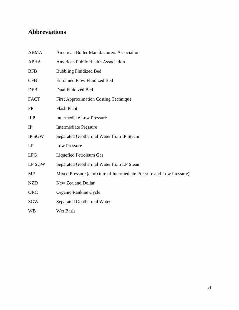
Abbreviations
ABMA American Boiler Manufacturers Association
APHA American Public Health Association
BFB Bubbling Fluidized Bed
CFB Entrained Flow Fluidized Bed
DFB Dual Fluidized Bed
FACT First Approximation Costing Technique
FP Flash Plant
ILP Intermediate Low Pressure
IP Intermediate Pressure
IP SGW Separated Geothermal Water from IP Steam
LP Low Pressure
LPG Liquefied Petroleum Gas
LP SGW Separated Geothermal Water from LP Steam
MP Mixed Pressure (a mixture of Intermediate Pressure and Low Pressure)
NZD New Zealand Dollar
ORC Organic Rankine Cycle
SGW Separated Geothermal Water
WB Wet Basis

xii
List of Figures
Figure 1. The annual electricity generation in New Zealand from 1976 to 2014 by fuel type[5]. . 1
Figure 2. A simplified schematic of a two flash geothermal power plant. ..................................... 3
Figure 3. A typical temperature-entropy state diagram for a two flash geothermal power plant,
modified from [11]. ................................................................................................................. 4
Figure 4. The relative power generation costs for different energy sources in New Zealand [14] 5
Figure 5. The range of applicability of different gasifier types [19]. ............................................. 6
Figure 6. The Dual Fluidized Bed used at the University of Canterbury[20]. ................................ 7
Figure 7. The schematic for the steam extraction manifold of the Wairakei Geothermal System
[21] .......................................................................................................................................... 8
Figure 8. Schematic of the separated geothermal water manifold at the Wairakei Geothermal
System [21] ............................................................................................................................. 9
Figure 9. Schematic of the Wairakei Power Plant A and B Stations[22]. .................................... 11
Figure 10. A diagram of one of the two identical turbine cycles at the Te Mihi Power Station .. 12
Figure 11. Diagram of the Poihipi Rd Power Plant ...................................................................... 13
Figure 12. Diagram of one of the twin pair of binary plant cycles within the Wairakei Binary
Plant (Dotted lines represent pentane flow) [24] .................................................................. 14
Figure 13. The pressure drop at several steam extraction wells at the Wairakei Geothermal Field
[29] ........................................................................................................................................ 16
Figure 14. A simplified diagram of syngas fired superheating of geothermal steam prior to
utilization in a steam turbine. ................................................................................................ 21
Figure 15. A temperature entropy diagram for the superheating of geothermal steam modified
from [11]. .............................................................................................................................. 22
Figure 16. A diagram of using geothermal steam turbine condensate as feed water to a syngas
fired boiler ............................................................................................................................. 24
Figure 17. Mollier Diagram illustrating the effect heating separated geothermal water has on
increasing the amount of water in the vapour phase, modified from [11]. ........................... 25
Figure 18. Diagram of the current steam and water flows at Flash Plant 14 ................................ 26
Figure 19. A diagram of performing fired heating on IP SGW for additional IP steam generation
............................................................................................................................................... 27
Figure 20. The Power Generation of the Wiarakei Binary Plant for 2015 ................................... 28
Figure 21. Diagram of heating additional SGW for use in the Wairakei Binary Plant ................ 29
Figure 22. Overview of the dual fluidized bed gasifier UniSim model, taken from Puladian's
Thesis [43] ............................................................................................................................ 31
Figure 23. The daily average valve positions for two bypass valves, PRV1 and PRV4 .............. 37
Figure 24. The estimated flowrates of IP steam bypassing through PRV1 and PRV4 ................. 38
Figure 25. The estimated bypassing steam calculated using IP steam flow estimates within and
measured IP steam input to the Wairakei A and B Stations ................................................. 39
Figure 26. The estimated bypassing steam based on both the estimated unused IP steam, and the
pressure relief valve positions ............................................................................................... 40
Figure 27. The power generation from the three LP turbines at Wairakei ................................... 41
Figure 28. The total steam input to the Wairakei A and B Stations, and the estimated bypassing
steam ..................................................................................................................................... 44

xiii
Figure 29. Entropy-Enthalpy diagram for steam in a MP turbine, for saturated IP steam (blue),
and steam superheated to 350°C (red) .................................................................................. 46
Figure 30. Numbered streams of steam and SGW around the modified FP14 ............................. 48
Figure 31. Power Output Correction Factors for the Wairakei Binary Plant with Separated
Geothermal Water inlet temperature. .................................................................................... 51
Figure 32. The mass flowrate of SGW feed to the Wairakei Binary Plant, and the estimated
amount of SGW bypassing the Binary Plant. ....................................................................... 52
Figure 33. Power output correction factors for the Wairakei Binary Plant with separated
geothermal water flowrate to the Binary Plant. .................................................................... 53
Figure 34. The additional SGW from T-Line that may be added to the feed of the Binary Plant
and the resultant total SGW flowrate .................................................................................... 54
Figure 35. The Power Generation of the Wairakei Binary Plant for 2015 and the estimated power
generation by heating and adding additional SGW from T-Line ......................................... 55
Figure 36. The heat requirement and associated biomass input in order to heat additional SGW in
T-line ..................................................................................................................................... 55
Figure 37. The permissible amount of silica in the boiler water in order to produce steam with a
silica content of 10 and 20 ppb [40]...................................................................................... 58
Figure 38. Diagram of apparatus used to minimize oxygen contamination during dissolved
oxygen sampling ................................................................................................................... 61
Figure 39. The solubility of oxygen in water under different temperatures and pressures [40] ... 68
Figure 40. The daily average of Poihipi Rd condensate flow to Te Mihi ..................................... 71
Figure 41. The delivered costs for landing residues for different delivery distances, assuming 8
GJ/m3 [66] ............................................................................................................................. 72
Figure 42. Yearly average prices for radiata pine pulp logs in New Zealand [68] ....................... 73
Figure 43. The distribution of planted forests in the North Island as of 2008, modified from [69].
............................................................................................................................................... 74
Figure 44. The wholesale prices of power used for the economic evaluations of the hybrid
configurations ....................................................................................................................... 77
Figure 45. Diagram of a disc chipper [73] .................................................................................... 80
Figure 46. A diagram of a drum chipper [73] ............................................................................... 81
Figure 47. A diagram of a hammer mill hog [73] ......................................................................... 81
Figure 48. Diagram of a cascade co-current rotary drum dryer [79] ............................................ 83
Figure 49. A cross section of a cascade rotary drum dryer [79] ................................................... 83
Figure 50. The biomass feed preparation and storage equipment ................................................ 84
Figure 51. The estimated cost (December 2004 NZD) for belt and bucket conveyors based on the
FACT Method ....................................................................................................................... 85
Figure 52. The estimated cost (December 2004 NZD) for auger and apron conveyors based on
the FACT Method ................................................................................................................. 86
Figure 53. The estimated cost (December 2004 NZD) for electric motors based on the FACT
Method .................................................................................................................................. 87
Figure 54. The estimated cost (1st Quarter 1998 USD) for furnaces based on the heat duty of the
furnace [90] ........................................................................................................................... 91
Figure 55. The estimated cost (1st Quarter 1998 USD) for packaged steam boilers based on the
steam production capacity [90] ............................................................................................. 96
Figure 56. The estimated cost (December 2004 NZD) for steam boilers based on the heating duty
[71]. ....................................................................................................................................... 97

xiv
Figure 57. The installed capital cost breakdown for modifying two MP turbines to utilize
superheated steam in Scenario 1 and Scenario 2 ................................................................ 109
Figure 58. The cumulative discounted cash flow for modifying two MP turbines to utilize
superheated steam in Scenario 1 ......................................................................................... 109
Figure 59. Sensitivity analysis for modifying two MP turbines to utilize superheated steam in
Scenario 1............................................................................................................................ 110
Figure 60. The cumulative discounted cash flow for modifying two MP turbines to utilize
superheated steam in Scenario 2 ......................................................................................... 112
Figure 61. Sensitivity analysis for modifying two MP turbines to utilize superheated steam in
Scenario 2............................................................................................................................ 113
Figure 62. The installed cost breakdown for modifying two MP turbines to utilize superheated
steam in Scenario 3 ............................................................................................................. 114
Figure 63. The cumulative discounted cash flow for modifying two MP turbines to utilize
superheated steam in Scenario 3 ......................................................................................... 114
Figure 64. Sensitivity analysis for modifying two MP turbines to utilize superheated steam in
Scenario 2............................................................................................................................ 115
Figure 65. The installed cost breakdown for using Poihipi Rd condensate as boiler feed water in
Scenario 1............................................................................................................................ 117
Figure 66. The cumulative discounted cash flow for using Poihipi Rd condensate as boiler feed
water in Scenario 1.............................................................................................................. 117
Figure 67. Sensitivity analysis for using Poihipi Rd condensate as boiler feed water in Scenario 1
............................................................................................................................................. 118
Figure 68. The installed capital cost breakdown for using Poihipi Rd condensate as boiler feed
water in Scenario 2.............................................................................................................. 119
Figure 69. The cumulative discounted cash flow for using Poihipi Rd condensate as boiler feed
water in Scenario 2.............................................................................................................. 120
Figure 70. Sensitivity analysis for using Poihipi Rd condensate as boiler feed water in Scenario 2
............................................................................................................................................. 121
Figure 71. The cumulative discounted cash flow for using Poihipi Rd condensate as boiler feed
water in Scenario 3.............................................................................................................. 122
Figure 72. Sensitivity analysis for using Poihipi Rd condensate as boiler feed water in Scenario 1
............................................................................................................................................. 123
Figure 73. The breakdown of the installed capital costs for using IP SGW from FP14 to generate
additional steam in Scenario 1 ............................................................................................ 124
Figure 74. The cumulative discounted cash flows for generating additional steam by boiling IP
SGW from FP14 in Scenario 1 ........................................................................................... 125
Figure 75. Sensitivity analysis for generating additional steam fusing IP SGW from FP14 as feed
water in Scenario 1.............................................................................................................. 126
Figure 76. The breakdown of the installed capital costs for using IP SGW from FP14 to generate
additional steam in Scenario 2 and Scenario 3 ................................................................... 127
Figure 77. The cumulative discounted cash flows for generating additional steam by boiling IP
SGW from FP14 in Scenario 2 ........................................................................................... 127
Figure 78. Sensitivity analysis for using Poihipi Rd condensate as boiler feed water in Scenario 2
............................................................................................................................................. 128
Figure 79. The cumulative discounted cash flows for generating additional steam by boiling IP
SGW from FP14 in Scenario 3 ........................................................................................... 129

xv
Figure 80. Sensitivity analysis for using Poihipi Rd condensate as boiler feed water in Scenario 3
............................................................................................................................................. 130
Figure 81. The breakdown of the installed capital costs for generating additional power by
heating makeup SGW for the Binary Plant ......................................................................... 132
Figure 82. The cumulative discounted cash flows for generating additional power by heating
makeup SGW for the Binary Plant for Scenario 1 .............................................................. 132
Figure 83. Sensitivity analysis for generating additional power by heating makeup SGW for the
Binary Plant for Scenario 1 ................................................................................................. 133
Figure 84. The cumulative discounted cash flows for generating additional power by heating
makeup SGW for the Binary Plant for Scenario 2 .............................................................. 134
Figure 85. Sensitivity analysis for generating additional power by heating makeup SGW for the
Binary Plant for Scenario 2 ................................................................................................. 135
Figure 86. The industrial natural gas prices in New Zealand from 1999-2015 [101] ................ 140

xvi
List of Tables
Table 1. The tolerances of internal combustion engines and gas turbines to various contaminants
present in syngas [34]. ......................................................................................................... 20
Table 2. The steam flows for the steam turbines at the Wairakei Power Plant operating at full
load ........................................................................................................................................ 36
Table 3. The no load steam flows and power generation rates for the steam turbines at the
Wairakei A and B Stations. ................................................................................................... 36
Table 4. The assumed flow coefficients for 20" butterfly valves [50] ......................................... 37
Table 5. The predicted mass flowrates of steam through each stage in a MP turbine, and the
resulting power generation for saturated steam at 150°C and 4.5 bara and superheated steam
at 350°C and 4.5 bara ............................................................................................................ 46
Table 6. ASME guidelines for feed water quality in modern industrial water tube boilers for
reliable continuous operation [40] ........................................................................................ 57
Table 7. ASME guidelines for boiler water quality in modern industrial water tube boilers for
reliable continuous operation [40] ........................................................................................ 58
Table 8. The contaminant testing method and detection limits for the tests performed on the
geothermal waters ................................................................................................................. 62
Table 9. The results for the sample impurities for the Poihipi Rd condensate, Te Mihi blowdown,
and Ohaaki blowdown performed by Hill Laboratories ....................................................... 63
Table 10. The measured dissolved oxygen for the geothermal waters ......................................... 63
Table 11. The hardness of the different sources of water. ............................................................ 64
Table 12. Boiler feed water impurities, their effects and removal [40] ........................................ 66
Table 13. The calculated blowdown required to mitigate problems that may be caused by silica,
TDS, and alkalinity in order to ensure safe boiler operation. ............................................... 69
Table 14. Testing results for the species of interest in Poihipi Rd condensate to assess the
variability of the condensate ................................................................................................. 70
Table 15. Manufacturer’s data for wood chip transfer screw conveyers [86] .............................. 86
Table 16. The assumed superficial gas velocities for the University of Canterbury’s dual
fluidized bed gasifier............................................................................................................. 88
Table 17. The estimated costs of recertifying turbines at the Wairakei Power Plant ................... 89
Table 18. The cost correction factors for centrifugal fans [71]. ................................................... 92
Table 19. The cost of pumps and motors for single stage pumps [71]. ........................................ 94
Table 20. Heat flux typical for different types of heat exchange in tubular heat exchangers [71] 95
Table 21. The prices for heat exchangers based on their design pressures [71]. .......................... 95
Table 22. Costs associated with purchasing and installing process equipment based on the
equipment cost [71]............................................................................................................... 98
Table 23. Pressure ratios and associated compressibility factors for centrifugal air fans [40]. .. 100
Table 24. Results for modifying two MP turbines to utilize superheated steam in Scenario 1 .. 108
Table 25. The cash flow summary for superheating geothermal steam in Scenario 1, all values
given in $1000’s .................................................................................................................. 110
Table 26. Results for modifying two MP turbines to utilize superheated steam in Scenario 2 .. 111
Table 27. The cash flow summary for superheating geothermal steam in Scenario 2, all values
given in $1000’s .................................................................................................................. 112

xvii
Table 28. Results for modifying two MP turbines to utilize superheated steam in Scenario 23 113
Table 29. The cash flow summary for superheating geothermal steam in Scenario 1, all values
given in $1000’s .................................................................................................................. 115
Table 30. Results for generating steam from Poihipi Rd condensate in Scenario 1 ................... 116
Table 31. The cash flow summary for using Poihipi Rd condensate as boiler feed water n
Scenario 1, all values given in $1000’s .............................................................................. 118
Table 32. Results for generating steam from Poihipi Rd condensate in Scenario 2 ................... 119
Table 33. The cash flow summary for using Poihipi Rd condensate as boiler feed water n
Scenario 2, all values given in $1000’s .............................................................................. 120
Table 34. Results for generating steam from Poihipi Rd condensate in Scenario 1 ................... 121
Table 35. The cash flow summary for using Poihipi Rd condensate as boiler feed water n
Scenario 3, all values given in $1000’s .............................................................................. 122
Table 36. Results for generating steam using IP SGW from FP14 in Scenario 1 ...................... 123
Table 37. The cash flow summary for boiling IP SGW from FP14 in Scenario 1, all values given
in $1000’s............................................................................................................................ 125
Table 38. Results for generating steam using IP SGW from FP14 in Scenario 2 ...................... 126
Table 39. The cash flow summary for boiling IP SGW from FP14 in Scenario 2, all cash values
given in $1000’s .................................................................................................................. 128
Table 40. Results for generating steam using IP SGW from FP14 in Scenario 3 ...................... 129
Table 41. The cash flow summary for boiling IP SGW from FP14 in Scenario 3, all values given
in $1000’s............................................................................................................................ 130
Table 42. Results for generating additional power by heating makeup SGW for the Binary Plant
for Scenario 1 ...................................................................................................................... 131
Table 43. Cash flow analysis for generating additional power by heating makeup SGW for the
Binary Plant in Scenario 1, all values given in $1000’s ..................................................... 133
Table 44. Results for generating additional power by heating makeup SGW for the Binary Plant
for Scenario 2 ...................................................................................................................... 134
Table 45. Cash flow analysis for generating additional power by heating makeup SGW for the
Binary Plant in Scenario 2 and Scenario 3, all cash values given in $1000’s .................... 135
Table 46. The breakeven prices of landing residues for the hybrid configurations .................... 139

1
1.0 Introduction
Due to declining fossil fuel reserves and the evidence of environmental damage and global
warming caused by fossil fuel use; renewable energy technologies are being increasingly utilized
to supply the growing demand for power [1]. Countries are committing to reducing climate
warming emissions, with recently two of the largest emitting countries, the USA and China,
ratifying the Paris agreement to curb climate warming emissions [2]. This will certainly increase
the demand for renewable energy sources.
New Zealand has historically generated a large proportion of its electricity from renewable energy
sources; with approximately 80% of the electricity generation in New Zealand coming from
renewable sources in 2014. This is due mainly to the utilization of hydro and geothermal resources
as can be seen in Figure 1.
The consumption of electricity in New Zealand has more than doubled since 1975 [3], though the
electricity demand has been seen to stagnate in recent years. This flattening of demand is attributed
to plant closures in the high energy use area such as pulp and paper, better insulation and more
efficient electrical appliances [4].
Figure 1. The annual electricity generation in New Zealand from 1976 to 2014 by fuel type[5].
Flat demand and a competitive electricity market has resulted in some displacement of less
efficient energy sources with more efficient and renewable sources, such as wind and Geothermal
[4]. This trend can be expected to continue with increased awareness of climate change and the
gradual depletion of fossil fuels.
Although electricity demand has been flat over the last few years there is the potential for demand
to grow significantly over the next decade or so. This demand would be driven by the transport
industry converting from a non-renewable fuel base to electric vehicles. It would be desirable to

2
meet this increased electricity demand with renewable power generation. There may be a need to
implement this additional renewable generating capacity relatively quickly, depending on the rate
of electric vehicle uptake.
The following sections aim to introduce:
Technical and economic aspects of both geothermal energy and gasification
The relevant features of existing geothermal power stations in the Wairakei geothermal
field
Technical and economic features of hybrid power generation
The rationale for this investigation
1.1 Geothermal Energy
Geothermal energy has been utilized for thousands of years in the form of hot springs, while
geothermal power generation has been performed since the early 1900s. Geothermal energy is the
heat of the earth and is present around the world, though high temperature geothermal resources
can only be found in places where the geology permits the transference of heat from the Earth’s
mantle to the crust. This generally only occurs when seismic activity causes distortions or fractures
in the Earth’s crust [6]. Where high temperature geothermal resources meet water reservoirs in the
ground, hot water and steam are produced. Geothermal power generation is most commonly
achieved by using geothermal steam to drive turbines which generate electricity.
Geothermal resources are defined as being dry or wet, depending on if there is liquid present in
the geothermal reservoir. If the geothermal resource is dry, then the geothermal steam extracted
may be directly passed through steam turbines for power generation. Dry steam plants are
generally simpler and less expensive than two-phase steam plants, and account for 26% of global
geothermal power production as of 2007 [7]. Two-phase steam plants utilize wet geothermal
resources that have both liquid and gas in the geothermal fluid; generally this fluid is separated so
the steam may be used with a steam turbine. Fluid separation usually occurs in a single or two
steps of flash separation, two-phase steam plants account for the majority of global geothermal
power generation, with 42% of geothermal power generation coming from single flash plants, and
23% of power generation coming from double-flash plants.
A simplified schematic of a two flash plant producing energy from extracting two-phase
geothermal fluid, separating the liquid and vapour components, and using the steam to drive a
turbine is displayed in Figure 2. As can be seen, intermediate pressure (IP) steam is separated from
the two-phase geothermal fluid, the resulting separated geothermal water (SGW) is then reduced
in pressure, and additional low pressure (LP) steam is generated in a second separator.
Two-flash separation allows for more complete utilization of the steam, however it does require
additional process equipment in the form of a second turbine and separator. The remaining SGW
and the condensate formed from condensing the steam at the back end of the LP turbine may then
be reinjected into the reservoir, or otherwise disposed of.

3
IP Separator
LP Separator
Extraction Well Reinjection Well
Condenser
LP Turbine
IP Turbine
Separated Geothermal Water
LP Steam
IP Steam
Two-phase fluid
Figure 2. A simplified schematic of a two flash geothermal power plant.
Geothermal energy has been used for electricity production on an industrial scale for over 50 years,
and has been developed into an important form of power generation, especially in New Zealand.
As of May 2007 there were 23 countries utilizing geothermal power generation over 504 sites to
produce over 9500 MW [8]. New Zealand has historically been a world leader in geothermal power
generation; with the first industrial scale developments to utilize liquid dominated geothermal
resources being implemented at Wairakei in the Taupo Volcanic Zone. The installed capacity at
Wairakei was initially 47 MW, however due to expansions and redesigning certain parts of the
plant, the installed capacity at Wairakei has varied throughout the plants operation, peaking at 172
MW [9]. Several power plants operate utilizing steam from the Wairakei Geothermal Field, which
currently provides geothermal steam to several power stations: Wairakei A, Wairakei B, Te Mihi,
and Poihipi Rd. There are also two binary plants operating on the Wairakei Geothermal Field, the
Wairakei and Te Huka Binary Plants, which generate power using organic Rankine cycles (ORC).
The thermodynamic process of a two flash geothermal power plant is displayed on a Mollier
diagram in Figure 3. The numbered labels on Figure 3 represent the different states of the
geothermal fluid throughout the process of generating power from the geothermal fluid. Power is
generated from the two-phase fluid by the following steps:
The two-phase geothermal fluid is extracted from the wellhead at State 1
The fluid is flashed as it enters the first stage separator, decreasing its pressure to State 2
The geothermal fluid is then separated in the separator into the liquid and vapour
components at State 3 and State 6 respectively
The separated liquid is then passed to the second stage separator, and again flashed to a
lower pressure at State 4
The lower pressure geothermal fluid is then separated into its liquid and vapour
components at State 5 and State 7 respectively
The SGW at State 5 can then be used in an organic Rankine cycle plant to generate
additional power, reinjected to the geothermal reservoir, or otherwise disposed of
The high pressure steam is expanded from State 6 to State 7 using a turbine
The low pressure steam at State 7 is then expanded across a second turbine to State 8

4
The resulting low quality steam at State 8 is condensed to State 9, where the condensate
may be disposed of or otherwise used on the plant [10].
Figure 3. A typical temperature-entropy state diagram for a two flash geothermal power plant, modified from
[11].
Geothermal energy is considered to be renewable as the heat extracted from the Earth is small
compared to the Earth’s large heat content. Geothermal energy does however usually produce
emissions of greenhouse gasses due to non-condensable gasses being desorbed from the
geothermal fluid. Though, these emissions are generally much lower than most alternatives for
energy production. Geothermal power plants have been seen to have a median of 38 gCO2eq/kWh,
in comparison; coal and gas power plants have been seen to have median emissions of 820
gCO2eq/kWh and 490 gCO2eq/kWh respectively [12]. Geothermal resources can also be utilized
in a binary power plant, which can theoretically have zero direct greenhouse gas emissions, though
in reality venting of CO2 is generally performed [13].
1.1.1 The Relative Cost of Geothermal Power Production
A further point to put the attractiveness of geothermal electricity generation into perspective is the
relative cost of new generating capacity compared to other renewable and non-renewable sources,
as displayed in Figure 4 [14]. It is clear that geothermal is one of the cheapest electricity generation
sources.

5
Figure 4. The relative power generation costs for different energy sources in New Zealand [14]
1.2 Gasification
Gasification is the process of converting a carbonaceous fuel to a gas with a usable heating value;
this gas is called: synthesis gas, syngas, or producer gas. In this study the gas produced from
gasification will be called syngas. During gasification, partial oxidation generally occurs to the
gasification feedstock creating H2 and CO, of varying ratios within the syngas. The produced
syngas can be burned directly to produce heat, used to produce work by using a gas engine or a
gas turbine, or refined into liquid fuels. Coal was the first feedstock used for industrial gasification,
though gasifiers have been developed so that they may produce syngas from biomass and waste
products. If biomass is used as the feedstock for gasification then the process is considered to be
renewable, and can have minimal emissions. Provided there is regrowth or replanting of the
feedstock biomass, then any CO2 emitted from the burning of syngas will be balanced by a
corresponding amount of absorbed CO2 by the biomass during its growth. Therefore, biomass
gasification is considered to be at worst, a carbon neutral form of energy production [15],[16].

6
Biomass gasification can exist in conjunction with other industrial activities, such as forestry, as
there are often large quantities of biomass that are by-products or waste products [17].
Within gasifiers, a range of different reactions occur in order to convert biomass feed into
combustible gasses. The reactions can be split into four steps within the gasification process;
drying, pyrolysis, combustion, and gasification. Drying is the process of vaporizing water within
the biomass. The moisture content of woody biomass can be as large as 50% by weight on a wet
basis (WB), while most gasifiers require moisture content within the range of 10-20% (WB).
Therefore, the majority of biomass drying required to be performed prior to feeding the biomass
into the gasifier. The remainder of the moisture content of the biomass is removed in the gasifier
as the biomass is heated to approximately 200°C. As the dried biomass is heated to above 230°C,
pyrolysis occurs which decomposes the biomass into volatile gasses, char, and tars. If the gasifier
is operated with air or oxygen as the gasification agent, then combustion of carbon and hydrogen
will occur, providing heat for gasification. The gasification step has several different reactions
occurring; the rates of these reactions are determined by the reaction conditions and type of feed
to the gasifier. The reaction rates of the different reactions in the gasification step can serve to
determine the composition of the syngas [18].
Gasification can occur in several different types of gasifiers, with fixed or fluidized bed material,
and with updraft or downdraft flow configurations. The range of applicability for different gasifier
types is represented in Figure 5, based on the thermal input of the feedstock to the gasifier. The
type bed material used within the gasifier can also be selected in order to aid in gasification, with
some bed materials acting as catalysts to the reactions being carried out within the gasifier.
Figure 5. The range of applicability of different gasifier types [19].
1.2.1 University of Canterbury’s Gasifier
At the University of Canterbury research into gasification is being performed on a promising type
of gasifier called a dual fluidized bed (DFB) gasifier, which consists of two fluidized beds. The
combustion of char and makeup fuel occurs in the first fluidized bed which is an entrained flow
fluidized bed (CFB), which then passes heated bed material to the second fluidized bed; a bubbling
fluidized bed (BFB), which uses the high temperature bed material to provide the necessary heat
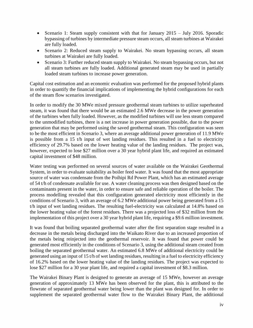
for the gasification reactions. Figure 6 illustrates the flow paths of the biomass, air, steam, flue
gas, and syngas within the gasification system.
7
Figure 6. The Dual Fluidized Bed used at the University of Canterbury[20].
The majority of the heat required by the DFB gasifier is provided by the combustion of the char
content of the biomass in the CFB, though some additional fuel is required. LPG is used as the
makeup fuel for the University of Canterbury’s DFB gasifier, recycled syngas could also be used
to provide the additional heat for gasification.
1.3 Wairakei Geothermal Field
The existing electricity generation plant at Wairakei utilizes a liquid dominated geothermal
reservoir, and predominantly two-stage flash separation is used prior to piping the steam to the
steam turbines. The Wairakei Steam Field Schematic is displayed in Figure 7, showing the steam
manifold joining the Wairakei A, Wairakei B, Te Mihi, and Poihipi Rd Power Stations. There is
also the nearby Ohaaki Geothermal Power Station, which is also owned by Contact Energy, but
does not utilize the Wairakei Geothermal Field
A large amount of separated geothermal water (SGW) is produced by separating steam from the
two-phase fluid extracted from the reservoir. As the SGW is still at high temperatures some SGW
is used to provide heating to other companies such as a prawn farm and local hot pools. SGW is
also used to provide the heat for the Wairakei Binary Plant. The SGW is disposed of either by
reinjection or by draining into the Waikato River. The schematic for SGW use and disposal on the
Wairakei Geothermal Field is displayed in Figure 8.

8
Figure 7. The schematic for the steam extraction manifold of the Wairakei Geothermal System [21]

9
Figure 8. Schematic of the separated geothermal water manifold at the Wairakei Geothermal System [21]

10
1.3.1 Wairakei A and B Power Stations
The oldest Power Station on the Wairakei Geothermal Field, the Wairakei A and B Stations were
commissioned in 1958. Currently, there are 8 steam turbines in operation at the Wairakei A and B
Stations. The current designed output for the Wairakei A and B Stations is 134.8 MWe. There are
four types of turbines at the Wairakei A and B Stations:
One intermediate pressure (IP) turbine, which generates 11.2 MWe at full load using IP
steam at 4.5 bara and exhausting LP steam at approximately 1.1 bara into the LP turbine
manifold
Three low pressure (LP) condensing turbines, which generate 11.2 MWe each at full load,
use LP steam at 1.1 bara, and produce condensate under vacuum conditions using water
from the Waikato River
Three mixed pressure (MP) condensing turbines which generate 30 MWe each at full load,
utilize steam at 4.5 bara and then 1.1 bara through different passes, and produce
condensate under vacuum conditions using Waikato River water
One Intermediate Low Pressure (ILP) turbine, which generate 4 MWe at full load, uses
steam at approximately 2.1 bara, and creates LP steam at its exhaust
The Wairakei A and B Stations, are displayed in Figure 9 [9]. The A and B Stations have
previously had a designed generation of 161.2 MWe, but the removal of an 11.2 MWe IP
turbine, G1 and an 11.2 MWe LP turbine, G8, has reduced the installed capacity.

11
Figure 9. Schematic of the Wairakei Power Plant A and B Stations[22].
1.3.2 The Te Mihi Power Station
The Te Mihi Power Station is the most recent addition to the Wairakei Geothermal Field, it was
opened in 2014 and is rated to produce a total of 166 MWe [23]. It uses two mixed pressure 83
MWe MP steam turbines that operate using a mixture of IP and LP steam. Direct contact
condensers are used in order to condense the steam at the back end of the turbines. The condensers
utilize water from cooling towers in order to perform condensation, which is predominantly
composed of Te Mihi condensate, though Poihipi Rd condensate is also added to the cooling tower
blowdown in order to regulate the water chemistry. A diagram of one of the two turbine cycles at
the Te Mihi Power Station is displayed in Figure 10.

12
LP Separator A
LP Separator B
LP Steam Scrubber A
LP Steam Scrubber B
IP Steam Scrubber
Steam Turbine
Condenser
Cooling Tower
Atmospheric flash tank
Poihipi Rd Condensate
LP SGW to reinjection
To holding pond and disposal
IP SGW
Figure 10. A diagram of one of the two identical turbine cycles at the Te Mihi Power Station
1.3.3 The Poihipi Rd Power Station
The Poihipi Rd Power Station was constructed in the mid-1990s as a joint venture between
Mercury Energy and Geotherm Energy, however it was acquired by Contact energy in 2000 [9].
Poihipi Rd has a single 55 MWe steam turbine that operates using IP steam from the Wairakei
Geothermal Field. Poihipi Rd is unique in the Wairakei Geothermal Field, as it uses a shell and
tube condenser to condense the geothermal steam at the back end of the turbine, as opposed to the
direct contact condensers used at the Wairakei A and B, and the Te Mihi Power Stations. As no
water from the Waikato River is mixed with the Poihipi Rd steam condensate and there is no
contact with the atmosphere, Poihipi Rd condensate is considered to be cleaner than that from the
direct contact condensers. A diagram of the Poihipi Rd Power Plant is displayed in Figure 11.

13
Demister
Steam Turbine
Condenser
Cooling Tower
Generator
Condensate to Te Mihi
Condensate
Cooling water
Cooling water return
IP steam
Figure 11. Diagram of the Poihipi Rd Power Plant
1.3.4 The Wairakei Binary Plant
The Wairakei Binary Plant was constructed in 2005 in order to generate additional power by
utilizing some of the high temperature SGW available in T-Line prior to its reinjection. The Binary
Plant consists of two twin power generating units, G15 and G16, which generate power using
pentane as the working fluid in organic Rankine cycles as displayed in Figure 12. G15 and G16
are designed to produce an average combined power output of 15 MWe, though this fluctuates
with changing ambient temperature, SGW flowrate, and SGW temperature, and has been as high
as 20 MWe. Currently silica scaling is observed within the plant, which serves to increase pressure
losses within the plant, and results in a reduction in the power generation of the Binary Plant, thus
silica removal is currently performed biannually.
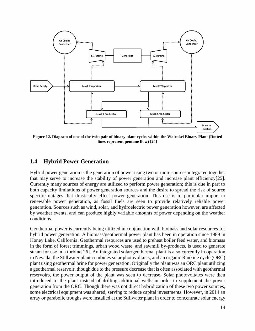
14
Figure 12. Diagram of one of the twin pair of binary plant cycles within the Wairakei Binary Plant (Dotted
lines represent pentane flow) [24]
1.4 Hybrid Power Generation
Hybrid power generation is the generation of power using two or more sources integrated together
that may serve to increase the stability of power generation and increase plant efficiency[25].
Currently many sources of energy are utilized to perform power generation; this is due in part to
both capacity limitations of power generation sources and the desire to spread the risk of source
specific outages that drastically effect power generation. This use is of particular import to
renewable power generation, as fossil fuels are seen to provide relatively reliable power
generation. Sources such as wind, solar, and hydroelectric power generation however, are affected
by weather events, and can produce highly variable amounts of power depending on the weather
conditions.
Geothermal power is currently being utilized in conjunction with biomass and solar resources for
hybrid power generation. A biomass/geothermal power plant has been in operation since 1989 in
Honey Lake, California. Geothermal resources are used to preheat boiler feed water, and biomass
in the form of forest trimmings, urban wood waste, and sawmill by-products, is used to generate
steam for use in a turbine[26]. An integrated solar/geothermal plant is also currently in operation
in Nevada; the Stillwater plant combines solar photovoltaics, and an organic Rankine cycle (ORC)
plant using geothermal brine for power generation. Originally the plant was an ORC plant utilizing
a geothermal reservoir, though due to the pressure decrease that is often associated with geothermal
reservoirs, the power output of the plant was seen to decrease. Solar photovoltaics were then
introduced to the plant instead of drilling additional wells in order to supplement the power
generation from the ORC. Though there was not direct hybridization of these two power sources,
some electrical equipment was shared, serving to reduce capital investments. However, in 2014 an
array or parabolic troughs were installed at the Stillwater plant in order to concentrate solar energy

15
to increase the temperature of the geothermal brine before entering the ORC plant. This addition
of solar thermal power generation adds 2 MWe to the power generation of the plant, and is
expected to slow the depletion of the geothermal reservoir. It has similarly been suggested that
concentrated solar thermal energy could be used in conjunction with biomass gasification in order
to provide the heat for gasification [27]. These hybrid power plants illustrate that different
renewable sources of power generation may be combined in order to attain a greater efficiency
than if each were utilized separately.
1.5 Reason for Investigation
Though gasification is a promising renewable technology which could serve to produce sustainable
combustible gas or liquid fuels if the syngas is further refined; there are very few commercial
biomass gasification plants globally. This is generally attributed to the relatively high cost of
biomass derived fuels compared to the fossil fuel alternatives. Biomass gasification is also not a
mature technology, and government support and clean energy incentives are generally required for
a biomass gasification plant to be considered commercially viable. However if the capital costs of
a biomass gasification plant can be reduced by hybridization with an existing plant, this may serve
to make the gasification plant viable. It is also possible that power generation using a hybrid
gasification/geothermal plant would have a higher efficiency than a standalone biomass electricity
generation plant, as this is commonly the case with hybrid power plants[28].
Contact Energy owns and operates several geothermal power plants in the Taupo Volcanic Zone
in the Central North Island of New Zealand. During the utilization of the Wairakei field, there has
been a significant decrease in the pressure of the reservoir as displayed in Figure 13. Though, the
reservoir pressure has been increasing since 1997 with part of this attributed to the in-field injection
of the geothermal brine occurring [29]. In order to maintain the Wairakei Geothermal Field, steam
extraction limits are in place in order to regulate the amount of steam that can be utilized, to
maintain the pressure of the field and ensure subsidence does not occur [30].

16
Figure 13. The pressure drop at several steam extraction wells at the Wairakei Geothermal Field [29]
There are currently multiple power plants operating on the Wairakei Geothermal field, the
Wairakei A Station, the Wairakei B station, the Te Mihi Station, and the Poihipi Rd Station, all of
which are connected by a steam manifold. The Te Mihi and Poihipi Rd Stations are more recent
additions to the Wairakei Geothermal Field, and can more efficiently generate power from the
geothermal steam than the Wairakei A and B Stations. Because of this, the steam is generally used
preferentially at the Te Mihi and Poihipi Rd Stations to ensure maximum power generation. The
combination of the steam extraction limits imposed on the Wairakei Geothermal Field, and the
preferential utilization of steam at Te Mihi and Poihipi Rd, has caused there to be some unused
capacity for power generation at the Wairakei A and B Stations.
Due to the unused capacity at Wairakei, and the proximity of Wairakei to the largest area for
forestry in New Zealand; there may be a case for the retrofitting of the Wairakei plant or other
geothermal plants in this area with biomass gasifiers. This hybridization could serve to augment
the power generation at the geothermal plant, or used to reduce steam extracted from the
geothermal reservoir if the steam extraction becomes further limited.
In short, the salient factors relating to this study are as follows:
It is desirable to increase the proportion of electricity generated from renewable energy
sources
Geothermal electricity production is relatively cheap, renewable, and a proven technology
Geothermal steam fields often decrease in enthalpy over time, decreasing the electricity
generation possible utilizing the field
New Zealand has a large amount of currently unused biomass in the form of landing
residues in close proximity to geothermal power plants in the Central North Island
Hybrid Power Plants are generally more efficient that single fuel plants, as there is sharing
of infrastructure and opportunities to optimize efficiency
17
There are very few commercial gasification plants, and hybridization of biomass
gasification with a proven technology could act as an intermediate step in the
implementation of biomass gasification
Biomass gasification could be retrofitted to a geothermal power plant to; boost electricity
production, mitigate reservoir deterioration by reducing the steam extraction to achieve the
same power production, or a combination of these.
This investigation focuses on retrofitting the underutilised Wairakei Geothermal Stations
with biomass gasification facilities. Various design options are considered and an initial
economic analysis is performed.
18
2.0 Potential Hybrid Plant Configurations
There are a variety of ways of retrofitting an existing geothermal power plant to utilize syngas
generated in a biomass gasifier. Several different configurations for a hybrid geothermal/natural
gas power plant were discussed in a report by the Kingston, Reynolds, Thom, and Allardice
Consulting Company for the New Zealand Energy Research and Development Committee [31],
which may also be applicable for a geothermal/gasification hybrid plant. The majority of these
configurations were designed to superheat the geothermal steam after the vapour/liquid separation
step, and some involved the addition of a gas turbine to generate additional electricity in a
combined cycle. There has also been a study performed by Thain and DiPippo into the
hybridization of geothermal power generation, using a biomass boiler to provide additional heat
to the process [32]. However, these configurations proposed in these studies were related to
potential new hybrid plants, and therefore were unconstrained by the limitations associated with
retrofitting an existing geothermal plant.
2.1 Factors for Consideration
There are several sources of potential problems from hybridization that are common amongst the
different hybrid configurations. These factors are briefly explained in this Section, and expanded
on as required for the different configurations.
2.1.1 Dissolved Minerals
The deposition of mineral scale can occur in wells, separators, pipes, turbines, and heat exchangers
in a geothermal power plant. There are many types of minerals that are present in geothermal
waters that have the potential to form scale. However at the Wairakei Power Plant, silica is the
mineral that is seen to cause the most operational problems at the plant. This scaling can be an
obstacle for fluid flow, as it can cause pressure losses in pipes by reducing the diameter of flow
paths. The scale can often have a rough texture, increasing the pressure losses caused by the friction
of the fluids in the pipe contacting the walls of the pipes. The deposition or precipitation of solids
on heat exchanger surfaces is known as fouling. Fouling increases the thermal resistance of the
heat exchanger, as the mineral scale has a lower thermal conductivity than the heat exchanger
tubes. The removal of silica scale often necessitates plant shut down in order to clean the process
equipment of silica scale [24]. The problems encountered with silica and scaling geothermal power
plant may be exacerbated with the introduction of a gasifier to augment power generation to the
plant, due either to evaporative precipitation or decreasing solubility of the minerals in water
occurring with decreasing geothermal water temperature.

19
2.1.2 Dissolved Gasses
Geothermal fluids usually contain gases such as carbon dioxide, hydrogen sulphide, ammonia, and
methane with the concentration generally increasing with reservoir temperature, though it is highly
variable between geothermal fields. These gases can prove to be an environmental pollutant if they
are released directly, and can also affect the chemistry of the geothermal fluids that must be taken
into account with plant design. The hydrogen sulphide and carbon dioxide present in the
geothermal fluid are both known causes of plant corrosion [33]. Non-condensable gas removal
generally occurs during the condensation of the geothermal steam, in order to maintain the vacuum
conditions in the condenser. If hybridization is to occur, care must be taken to ensure the dissolved
gases in the geothermal fluids do not cause damage to the new and existing process equipment due
to changes in the plants operation.
2.1.3 Design Limitations of the Existing Plant
The fact that this study is concerned with the retrofitting of an existing geothermal power plant
with a biomass gasifier must be considered throughout the design process. Due to the plant design
and material selection of the existing plant, configurations that may be possible for a new hybrid
geothermal-gasification plant may not be practical to retrofit.
2.1.4 Syngas Purity
Syngas created in biomass gasifiers contains contaminants such as; particulates, tars, hydrogen
sulphide, carbon dioxide, nitrogen compounds, alkali compounds and chlorine compounds [34].
In order for syngas to be utilized in gas turbines or gas engines, cleaning will be required. With
removal of alkali, and sulphur compounds, particulates, tars, and chloride compounds from the
syngas needing to be performed [35].
According to Brown, the syngas produced from a dual fluidized bed gasifier will have
approximately 10 g/m3 of tars, and “high” particulate content from the gasifier [36]. The amount
of sulphur, nitrogen, and chloride contaminants in the syngas are dependent on the feed to the
gasifier. As it is most likely that any gasifier retrofitted at the Wairakei Power Station will have a
feed of landing residues due to the large amount of forestry in the Central North Island; woody
biomass is used as the basis for calculating the contaminants of the gasification syngas. It was
found that woody crops have a range of concentrations for nitrogen, sulphur, and chlorine of 0.06
– 0.6 wt. %, 0.01 – 0.02 wt. %, and 0.01 – 0.10 wt. % respectively [36].
The tolerance of fired boilers to the contaminants present in syngas is not known, though it is
expected that fired boilers will have a higher tolerance to the expected contaminants than internal
combustion engines and gas turbines. Some general contaminant tolerances for internal
combustion engines and gas turbines are displayed in Table 1.

20
Table 1. The tolerances of internal combustion engines and gas turbines to various contaminants present in
syngas [34].
Contaminant Unit IC Engine Gas Turbine
Particulate mg/m3 < 50 < 30
Tars mg/m3 < 100 < 8
Sulphur ppm - <20 Nitrogen ppm - <50
Alkali ppb - <24 Chloride ppm - <1
It is believed that using cyclones to remove the particulates from the syngas will be sufficient
cleaning if the syngas is to be utilized in a boiler or furnace, as direct combustion technologies are
much more resilient to contaminants compared to gas engines and gas turbines. Also, tars that are
present in the syngas will be able to be burnt by direct combustion, and provide some additional
heat for combustion. The precipitation of tars is not expected to occur, if the hot syngas is
combusted, however if this syngas stored or otherwise allowed to cool, tar precipitation may occur.
As it is assumed that syngas combustion will occur directly after syngas formation, this is not
expected to be an issue, but may need to be taken into account with shutdowns for plant
maintenance.
2.2 Superheating of Geothermal Steam
The superheating of the geothermal steam using gasification syngas is perhaps the simplest concept
of the different hybrid configurations. By superheating the geothermal steam, more electricity may
be generated with the same amount of steam, or alternatively less steam may be extracted from the
geothermal field to generate the same amount of electricity. The concept of superheating
geothermal steam is by no means a new one; it has been proposed from as early as 1924 by
Coufourier [37]. Originally geothermal hybrid configurations were generally concerned with using
fossil fuels to superheat geothermal steam; however in more recent years hybrid configurations
utilizing renewable energy sources have been investigated. An investigation into the superheating
of geothermal steam using natural gas at the Ohaaki (previously known as the Broadlands)
Geothermal Field was performed for the New Zealand Energy Research and Development
Committee by the Kingston, Reynolds, Thom and Allardice Consultancy [31]. More recently, the
idea of using a biomass boiler to superheat geothermal steam was investigated by Thain and
DiPippo [32].
As power generated from a steam turbine can be given by Equation 1 it can be seen that, as the
enthalpy of the input steam increases, the amount of work generated by the steam also increases,
provided the exit conditions of the steam turbine are not overly altered.
�̇�𝑺𝑻 = �̇�𝑺(𝒉𝒊𝒏 − 𝒉𝒐𝒖𝒕) (1)
Where:
�̇�𝑆𝑇 = the work performed by the steam turbine (kW)

21
�̇�𝑆 = the mass flowrate of steam to the turbine (kgs-1)
hin = the enthalpy of the steam at the inlet of the turbine (kJkg-1)
hout = the enthalpy of the steam at the outlet of the turbine (kJ/ kg-1)
Because of the increase in enthalpy of the steam due to superheating; the power generated by the
steam turbine will be increased by superheating the input steam. A simplified representation of the
superheating of geothermal steam using a syngas fired heat exchanger is shown in Figure 14. The
steam and gas requirements for the gasification section of the process will likely be sourced from
the geothermal steam, and a recycle stream on the syngas respectively.
IP Separator
LP SeparatorExtraction
Well Reinjection Well
Condenser
LP Turbine
IP Turbine
Separated Geothermal Water
Syngas
Steam
Biomass
Flue gasRecycled Syngas
DFB gasifier
Flue gas
Furnace
Figure 14. A simplified diagram of syngas fired superheating of geothermal steam prior to utilization in a
steam turbine.
The process of superheating geothermal IP steam for use in an IP steam turbine may be represented
on a temperature entropy diagram as shown in Figure 15. The superheated process is modified
from the current steam turbine cycle displayed in Figure 3 by the addition of the superheating from
State 6 to State 7 in Figure 15. The steam expansion from State 7 to State 8 is represented as the
ideal isentropic expansion, though this will not be the case in reality. The greater temperature drop
attained from turbine expansion in the superheated case compared to the base case will have a
correspondingly greater enthalpy drop; and consequently more power may be generated from the
steam turbine for the same mass flowrate of steam.
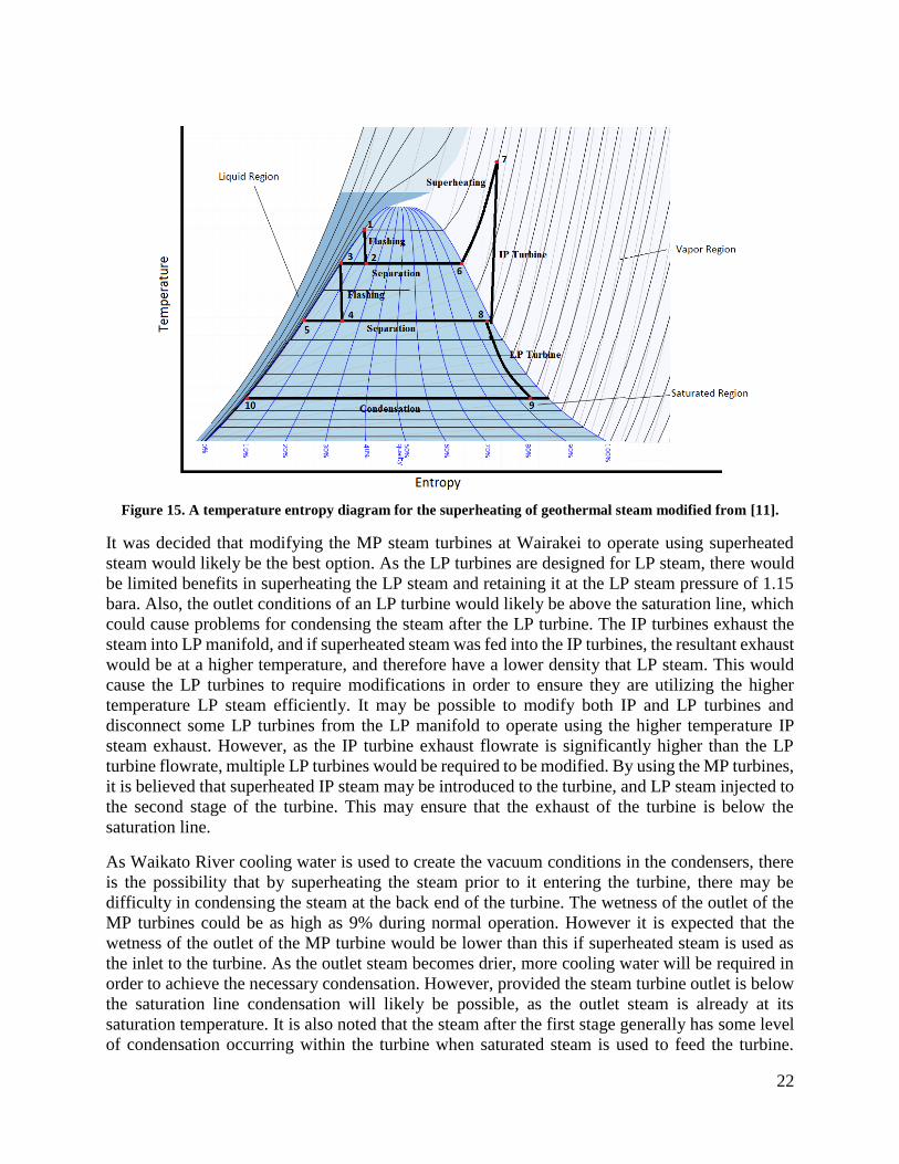
22
Figure 15. A temperature entropy diagram for the superheating of geothermal steam modified from [11].
It was decided that modifying the MP steam turbines at Wairakei to operate using superheated
steam would likely be the best option. As the LP turbines are designed for LP steam, there would
be limited benefits in superheating the LP steam and retaining it at the LP steam pressure of 1.15
bara. Also, the outlet conditions of an LP turbine would likely be above the saturation line, which
could cause problems for condensing the steam after the LP turbine. The IP turbines exhaust the
steam into LP manifold, and if superheated steam was fed into the IP turbines, the resultant exhaust
would be at a higher temperature, and therefore have a lower density that LP steam. This would
cause the LP turbines to require modifications in order to ensure they are utilizing the higher
temperature LP steam efficiently. It may be possible to modify both IP and LP turbines and
disconnect some LP turbines from the LP manifold to operate using the higher temperature IP
steam exhaust. However, as the IP turbine exhaust flowrate is significantly higher than the LP
turbine flowrate, multiple LP turbines would be required to be modified. By using the MP turbines,
it is believed that superheated IP steam may be introduced to the turbine, and LP steam injected to
the second stage of the turbine. This may ensure that the exhaust of the turbine is below the
saturation line.
As Waikato River cooling water is used to create the vacuum conditions in the condensers, there
is the possibility that by superheating the steam prior to it entering the turbine, there may be
difficulty in condensing the steam at the back end of the turbine. The wetness of the outlet of the
MP turbines could be as high as 9% during normal operation. However it is expected that the
wetness of the outlet of the MP turbine would be lower than this if superheated steam is used as
the inlet to the turbine. As the outlet steam becomes drier, more cooling water will be required in
order to achieve the necessary condensation. However, provided the steam turbine outlet is below
the saturation line condensation will likely be possible, as the outlet steam is already at its
saturation temperature. It is also noted that the steam after the first stage generally has some level
of condensation occurring within the turbine when saturated steam is used to feed the turbine.
23
However, if superheated steam is used, this condensation will likely not occur within the first stage
of the turbine. As there is an allowance for drainage to occur between stages in the geothermal
steam turbines, if no liquid is forming in the turbine, steam may start passing through these
drainage holes and causing erosion. This problem is addressed by Morris in his report on using
superheated steam in a saturated steam turbine, and he believes that filling these holes will not be
an issue, but will limit the ability to operate the turbines using the saturated steam [38].
It may be possible that by superheating the IP steam, evaporation of any liquid carryover present
in the geothermal steam will produce small flecks of precipitated minerals. These evaporate
particles will be extremely abrasive to the process equipment, and will likely cut into metal, as
these particles will be travelling at the same speed as the geothermal steam [38]. The evaporate
particles may be able to be eliminated from the feed by utilizing high efficiency separators, and
scrubbers to maintain good steam condition. However, currently the relatively large distances
between separators and turbines at Wairakei cause the majority of liquid carryover from the
separators to form on the walls of the steam lines, and are subsequently removed in drain pots.
2.3 Vaporization of Steam Turbine Condensate
In order to generate additional power from the Wairakei turbines, a boiler creating additional IP
steam could be used to supplement the existing geothermal steam supply. In order to reduce the
operating costs for the boiler, it would be advantageous to utilize water available on site as the
feed water. The majority of the water available at the Wairakei site is in the form of separated
geothermal water (SGW), and the high dissolved mineral content of the SGW would likely prove
to make the SGW unsuitable to be used as boiler feed water. This is due to the fact that silica scale
may form due to both evaporative precipitation, or by precipitation as the geothermal liquid cools,
thereby decreasing the solubility of silica in the water [39]. As the solubility of minerals in water
is generally much higher in the liquid phase than the gas phase; it may be possible to utilize the
steam condensate from the geothermal steam turbines as a source of boiler feed water, as the silica
and other minerals have been distilled from the condensate.
Even though the Wairakei A Station is currently the only station with capacity to utilize additional
steam on the Wairakei Geothermal Field, it is possible to position the boiler elsewhere on the steam
manifold and still utilize this unused capacity. Provided that the IP steam generated is fed into the
IP steam lines on the Wairakei Geothermal Field, any additional steam added to the system could
result in additional power generation at the Wairakei A Station. This is due to the fact that steam
is preferentially used at the Te Mihi and Poihipi Rd Power Stations; any additional steam input
into the steam manifold would simply result in less steam being diverted to be utilized at Te Mihi
or Poihipi Rd. This is of importance, as it allows sources of condensate other than that formed at
Wairakei to be used as boiler feed water in order to generate additional power at Wairakei. The
most suitable source of boiler feed water at the Wairakei Geothermal Field was therefore be
investigated in Section 4.0 to ensure that the costs associated with cleaning boiler feed water are
minimized.
A diagram of the plant configuration utilizing a syngas fired boiler to generate additional steam
from the steam turbine condensate is displayed in Figure 16. In order to maximize the steam
generation from the boiler, preheating of the geothermal condensate will be performed using SGW.

24
Though this configuration is expected to have a lower efficiency than other configurations, the fact
that it does not obstruct normal operation of the plant, or become integral to the operation of the
plant make this configuration more flexible than other configurations.
IP Separator
LP SeparatorExtraction
Well Reinjection Well
Condenser
LP Turbine
IP Turbine
Separated Geothermal Water
Syngas
Steam in
Biomass in
Flue gasRecycled Syngas
DFB gasifier
Flue gas
Boiler
Condensate
Additional IP Steam
Figure 16. A diagram of using geothermal steam turbine condensate as feed water to a syngas fired boiler
It is not only likely that the utilization of condensate for boiler feed water will serve to reduce the
risk of mineral scaling compared to utilizing the separated geothermal water; it may even reduce
the scaling that already occurs in the geothermal plant. The additional steam generated by
vaporizing the geothermal condensate will have a lower concentration of minerals that the IP
geothermal steam it is supplementing. This is due to the fact that the blowdown on the boiler will
serve to remove the majority of the influent minerals from the boiler [40]. Therefore,
implementation of the boiler will reduce the risk of mineral scaling downstream of the boiler. The
idea of avoiding silica deposition by dilution has been explored for silica saturated liquids [41],
however steam dilution to mitigate silica deposition has not been investigated, to this Author’s
knowledge. Mineral deposits are known to occur in geothermal steam turbines and are caused by
either liquid carry over or evaporated mineral [42]. Therefore, with the addition of supplementary
steam that has a lower mineral concentration than the geothermal steam would likely serve to
reduce mineral deposition in the geothermal steam turbines.
As it is planned to utilize separated geothermal water in order to preheat the steam turbine
condensate, the potential for mineral scaling in the preheater must be taken into account. As the
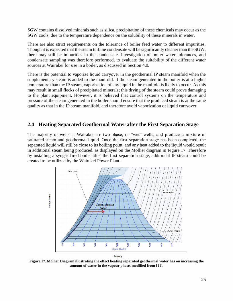
25
SGW contains dissolved minerals such as silica, precipitation of these chemicals may occur as the
SGW cools, due to the temperature dependence on the solubility of these minerals in water.
There are also strict requirements on the tolerance of boiler feed water to different impurities.
Though it is expected that the steam turbine condensate will be significantly cleaner than the SGW,
there may still be impurities in the condensate. Investigation of boiler water tolerances, and
condensate sampling was therefore performed, to evaluate the suitability of the different water
sources at Wairakei for use in a boiler, as discussed in Section 4.0.
There is the potential to vaporize liquid carryover in the geothermal IP steam manifold when the
supplementary steam is added to the manifold. If the steam generated in the boiler is at a higher
temperature than the IP steam, vaporization of any liquid in the manifold is likely to occur. As this
may result in small flecks of precipitated minerals; this drying of the steam could prove damaging
to the plant equipment. However, it is believed that control systems on the temperature and
pressure of the steam generated in the boiler should ensure that the produced steam is at the same
quality as that in the IP steam manifold, and therefore avoid vaporization of liquid carryover.
2.4 Heating Separated Geothermal Water after the First Separation Stage
The majority of wells at Wairakei are two-phase, or “wet” wells, and produce a mixture of
saturated steam and geothermal liquid. Once the first separation stage has been completed, the
separated liquid will still be close to its boiling point, and any heat added to the liquid would result
in additional steam being produced, as displayed on the Mollier diagram in Figure 17. Therefore
by installing a syngas fired boiler after the first separation stage, additional IP steam could be
created to be utilized by the Wairakei Power Plant.
Figure 17. Mollier Diagram illustrating the effect heating separated geothermal water has on increasing the
amount of water in the vapour phase, modified from [11].

26
The Wairakei Geothermal Field uses two-stage separation to produce IP and LP steam, and by
generating additional steam using the intermediate pressure separated geothermal water (IP SGW)
as a boiler feed the amount of LP steam generated would be decreased. This is due to the fact that
the overall mass of IP SGW is reduced if heat is added and IP steam produced, therefore reducing
the feed to the LP separators. However, there is a second stage separator at Wairakei that is limited
by the amount of LP steam it may produce, at Flash Plant 14 (FP14), which feeds to the Wairakei
A and B stations. The current configuration of FP14 is displayed in Figure 18.
Two-phase fluid
IP Steam (S -line & R-line)
IP SGW to drain
IP SGW to reinjection (T-line)
ILP Steam (G-line)
LP SGW to reinjection (X-Line)
LP SGW to drain
SGW to drain
IP SGW to FP14 ILP
FP14IP
FP14ILP
Figure 18. Diagram of the current steam and water flows at Flash Plant 14
By heating the separated fluid generated from the first stage separator, more IP steam may be
produced without necessarily reducing the amount of LP steam produced in the second separation
stage. The amount of additional IP steam that may be produced by heating the two-phase fluid is
relatively independent of the flowrate of two-phase fluid unless all of the liquid in the two-phase
fluid is being vaporized. Flash Plant 14 has a relatively large flowrate of two phase fluid entering
it, at approximately 2000 t/h, and the LP steam produced in the second stage of separation is limited
to 40 t/h, the hybridized flash plant 14 and IP SGW boiler configuration is displayed in Figure 19

27
Two-phase fluid
IP Steam(S-line & R-line)
IP SGW to drain
IP SGW to reinjection (T-line)
ILP Steam (G-line)
LP SGW to reinjection (X-Line)
LP SGW to drain
SGW to drain
IP SGW to FP14 ILP
FP14IP
FP14ILP
Additional IP Steam (R-line)
Steam
Biomass
Flue gas
Recycled Syngas
DFB gasifier
Syngas
Flue gas
Boiler
Boiler blowdown
Figure 19. A diagram of performing fired heating on IP SGW for additional IP steam generation
The possibility of heating the two-phase fluid prior to the IP separators was also investigated, as
this would simply increase the dryness of the two-phase fluid prior to the first stage of separation.
However, this would require a boiler using the two-phase fluid as the feed, which would decrease
the heat transfer efficiency of the boiler compared to a liquid feed to the boiler.
As the SGW after first stage separation has not been observed to exhibit silica scaling, even though
it has a silica content as high as 622 mg/kg, the boiler may be able to operate using the SGW as a
feed water. If a continuous blowdown is used, then it is believed that the silica concentration will
remain low enough to prevent scaling in the boiler, however it may cause increased scaling
downstream of the separation stage. Generally the blowdown of boilers is desired to be minimized
in order to prevent the loss of heated boiler water [40]. However, provided there is minimal heat
loss after the first separation stage, the SGW is already at its boiling point, a large continuous
blowdown may be used without excessive loss of heat, as the heat input should only produce
additional steam.
There may also be environmental benefits of implementing this configuration, as the amount of
arsenic and other metals entering the Waikato River will be reduced, due to an increased proportion
of the metals being reinjected. Currently the resource consent for discharging water to the Waikato
from Wairakei is based on the amount of arsenic entering the river. As the flowrates to the T-line
and X-line for reinjection are relatively constant, the amount of SGW entering the Waikato River
will be reduced by the overall decrease in SGW flowrate caused by the steam generation. As the
solubility of arsenic and other metals in the IP steam is negligible, the concentration of these metals
in the SGW will be increased due to the evaporation of water in the boiler. This increased
concentration will cause a greater proportion of the metals to be reinjected.

28
2.5 Heating Additional Separated Geothermal Water for Use in a Binary
Plant
There is the potential for syngas fired heating to be implemented within an existing binary plant at
Contact Energy’s Wairakei Power Plant. The binary plant currently uses SGW available at
approximately 130°C in the X-line prior to its reinjection. The Binary Plant was designed for an
average power generation of 15 MWe, however the actual observed average generation is
approximately 13MW, as is shown by the red line in Figure 20.
Figure 20. The Power Generation of the Wiarakei Binary Plant for 2015
The temperature of the SGW directly affects the amount of heating that may be performed on the
pentane, though this is limited by the design of the binary plant. As the binary plant is designed to
utilize SGW at 127 °C, there is limited benefit to further heating the SGW above this design
temperature. Similarly the flowrate of the SGW directly affects the amount of heating that can be
performed to the pentane, and limited benefits if the flowrate is raised above the design flowrate
of 2800 t/h.
Due to the fact that cooling is being performed on the silica laden SGW, and silica solubility
decreases with temperature; silica scaling is observed within the plant. The flowrate of SGW into
the binary plant is reduced as scaling increases due to an increase in frictional pressure losses.
Silica scaling also decreases the performance of heat exchangers within the plant, and therefore
reduces the power generation of the Binary Plant. Therefore silica removal using hydrofluoric acid
is currently performed biannually, in order to increase the power generation of the Binary Plant
[24].
As can be seen in Figure 20, the actual average power generation of the Wairakei Binary Plant is
approximately 2 MWe lower than the designed power generation of 15 MWe. This is attributed to
the average mass flow of SGW entering the binary plant being approximately 2300 t/h,
significantly lower than the designed flowrate of 2800 t/h. However, it is noted that even though

29
it appears that there is capacity for additional SGW being fed to the Binary Plant, SGW was
observed to bypass the binary plant for much of 2015. This bypassing is attributed to silica scaling
within the Binary Plant limiting the flowrate of SGW through the binary plant. It is assumed that
more frequent silica removal within the Binary Plant would solve this issue, though this will incur
additional costs.
The power output of the Binary Plant is seen to be dependent on several factors, the temperature
of the SGW, the flowrate of SGW, and the ambient air temperature. From this, the power output
of the binary plant may be increased by increasing the flow of SGW or by increasing the
temperature of the SGW. By performing heating on the SGW, more heat can be transferred to the
pentane working fluid. However as the designed entrance temperature of SGW to the stage 1
vaporizer is 127°C, and the current average temperature of SGW is 130°C, additional heating
would serve to further deviate the temperature of the SGW from the designed entrance
temperature. Increasing the flowrate of SGW to the binary plant would also serve to increase the
heat transfer to the pentane and result in increased power generation from the binary plant. The
only source of SGW available at 130°C is the X-line, and is already allocated to the binary plant,
however there is the option to utilize some lower temperature SGW available at approximately
105°C in the T-line. Even though it may be possible to generate additional power from the binary
plant without performing any additional heating, it is believed that mixing the two sources of silica
laden SGW may result in increased silica deposition within the binary plant. This is based on
observations made by Generation Engineers at Wairakei on silica scaling increasing in cases of
SGW mixing. Therefore, mixing the X-line SGW at 130°C with the T-line SGW at 105°C could
cause a greater amount of silica precipitation and exacerbate silica scaling in the binary plant.
However, by heating the SGW in the T-line from approximately 105°C to the same temperature
as the SGW in X-line at approximately 130°C; it is believed that this would likely avoid the issue
of increased silica precipitation, due to the increased solubility of silica in the higher temperature
water. The configuration of heating the SGW in T-line to provide additional SGW flowrate to the
Binary Plant is displayed in Figure 21.
Steam
Biomass
Flue gas
Recycled Syngas
DFB gasifier
Flue gas
Residual T-linefor reinjection
T- line SGW X-line SGW
Mixed SGW to binary plant
Heated make-upSGW
Syngas
Figure 21. Diagram of heating additional SGW for use in the Wairakei Binary Plant

30
3.0 Process Modelling of the Wairakei Geothermal System and
Hybrid Configurations
In order to evaluate the efficacy of the hybrid plant configurations, models were developed to
simulate some of the hybrid plants proposed in Section 2.2. A model for biomass gasification had
been created by Nargess Puladian during the course of her PhD at the University of Canterbury
using the heat and material balance software, UniSim [43]. This model could then be modified in
order to better suit the use of syngas for power generation instead of liquid fuel synthesis. Models
for the current Wairakei Geothermal Power Plant, and the additional process equipment required
to retrofit the Geothermal Power Plant with additional syngas fired heating were created using
UniSim.
3.1 Modelling Biomass Gasification
The gasification portion of the modelling encompasses the drying of the biomass, the combustion
of char and syngas in a combustion reactor, and the gasification reactor where pyrolysis and char-
gas reactions take place. As the models for gasification and biomass drying created by Puladian
during her PhD were originally designed to provide a syngas feed for Fischer-Tropsch synthesis
of liquid fuels, some modifications were performed to make these models suitable for power
generation using syngas.
3.1.1 Biomass Drying
In order to estimate the heat requirement for the biomass dryer, a modified version of Puladian’s
model for biomass drying was employed [43]. The biomass drying mechanism used by Puladian
was modelled in three steps using a macro module in UniSim: feed preheating, constant rate
drying, and falling rate drying. During feed preheating, the sensible heat of the flue gas drying
medium is transferred to the wet biomass raising the temperature of the biomass towards the wet
bulb temperature. Moisture in the wet biomass is rapidly evaporated during the constant rate
drying, as the drying rate is dominated by the heat transfer to the surface of the biomass. As the
biomass dries the drying rate falls due to the movement of moisture within the biomass towards
the biomass surface before evaporation occurs. However, as the final moisture content of the
biomass is still relatively high (15%), the drying rate is still relatively high at the end of the drying.
This causes the drying process to be largely controlled by the heat transfer to the biomass, and not
the mass transfer of moisture in the biomass.
The UniSim model created by Puladian to simulate the biomass drying was based on the overall
heat and mass balance equations of the biomass and the flue gas used as the drying medium, and
the following assumptions:
The temperature of the biomass and the drying medium at the outlet of the dryer is very
close. Rigorous modelling results have shown that the temperature difference at the dryer’s

31
outlet in co-current rotary dryer is insignificant when the final moisture content is less than
15 % as shown in Iguaz et al. [44] and Xu and Pang [45].
The exhaust gas temperature is always higher than the wet-bulb temperature of the flue gas
(70 ˚C).
The heat of vaporization of water is kept constant during the drying using the average
temperature between inlet and outlet temperatures.
The heat loss of the dryer is assumed to be 15 % based on the experimental results with a
semi-industrial rotary dryer reported in Meza et al. (2008). It does not include the heat loss
by the exhaust gas.
The amount of flue gas required for use as the drying medium could then be determined in order
to achieve the necessary drying. A controller function was implemented in UniSim to vary the
recycled syngas to the gasifier’s combustion reactor, and therefore the amount of high temperature
flue gas being generated in the reactor. This controller ensured that the flue gas and biomass outlet
temperature was 107°C from the rotary dryer; this would allow adequate drying of the biomass in
the dryer. This outlet temperature was the one used by Puladian in her thesis, and was concordant
with information published by NREL that typical dried biomass temperatures from rotary dryers
are between 71-110°C, though most exit temperatures are above 104°C in order to avoid
condensation of acids and resins[46].
3.1.2 Dual Fluidized Bed Gasifier
The dual fluidized bed gasifier was modelled in UniSim by Puladian in several stages: char and
syngas combustion, pyrolysis, and char-gas reactions. In Puladian’s thesis there was also a steam-
gas shift reactor, which was implemented to generate additional hydrogen to ensure the syngas
was suitable as an input for Fischer-Tropsch synthesis to a liquid fuel. The overview of Puladian’s
dual fluidized bed model is displayed in Figure 22.
Figure 22. Overview of the dual fluidized bed gasifier UniSim model, taken from Puladian's Thesis [43]
32
3.1.2.1 Char and Syngas Combustion
The heat required for the gasification reactions is supplied by the combustion of char, and often
some make up fuel in a combustion reactor. In this case some of the produced syngas would likely
be recycled to provide the additional heat for gasification. A conversion reactor was used to model
the combustion reactions, char and the components of syngas, hydrogen, carbon monoxide and
methane were combusted to generate heat for gasification and the hot flue gas for the drying
medium in the rotary dryer, as described by the reactions in Equations 2-5.
𝑪 + 𝑶𝟐 → 𝑪𝑶𝟐, ∆𝐻 = −3.9 × 10⁵ 𝑘𝐽/𝑘𝑚𝑜𝑙 (2)
𝑯𝟐 + 𝟏
𝟐𝑶𝟐 → 𝑯𝟐𝑶, ∆𝐻 = −2.4 × 10⁵ 𝑘𝐽/𝑘𝑚𝑜𝑙 (3)
𝑪𝑶 + 𝟏
𝟐𝑶𝟐 → 𝑪𝑶𝟐, ∆𝐻 = −2.8 × 10⁵ 𝑘𝐽/𝑘𝑚𝑜𝑙 (4)
𝑪𝑯𝟒 + 𝟐𝑶𝟐 → 𝑪𝑶𝟐 + 𝟐𝑯𝟐𝑶, ∆𝐻 = −8.0 × 10⁵ 𝑘𝐽/𝑘𝑚𝑜𝑙 (5)
3.1.2.2 Pyrolysis
During pyrolysis biomass is converted into char and combustible gasses. The major components
of the pyrolysis gas were determined by performing elemental balances on C, H, and O, and by
introducing two empirical factors, Φ𝐶𝑂 and Φ𝐶𝐻4. Where Φ𝐶𝑂 and Φ𝐶𝐻4
are the ratios of CO/CO2
and CH4/H2 respectively. By assuming that C, H, and O were only present in the 5 major
components of the pyrolysis gas: H2, H2O, CO, CO2, and CH4, the concentration of these
components in the pyrolysis gas could be determined. The empirical factors Φ𝐶𝑂 and Φ𝐶𝐻4 were
calculated using Equation 6 and Equation 7. These equations were developed by curve fitting of
the experimental data reported by Fagbemi et al [47].
𝚽𝑪𝑶 = 𝑨𝟏𝑬𝒙𝒑−𝑩𝟏
𝑻𝑮 (6)
𝚽𝑪𝑯𝟒= 𝑨𝟐𝑬𝒙𝒑
−𝑩𝟐
𝑻𝑮 (7)
Where:
TG = the gasification temperature (K)
A1 = an empirical constant (A1 = 4.7×10³)
B1 = an empirical constant (B1 = 7163.6)
A2 = an empirical constant (A2= 2.28×10⁻³)
B2 = an empirical constant (B2=5404.85)
33
The final tar content (dry basis) of the syngas was assumed to be a function of the gasifier
temperature, and the resulting function displayed in Equation 8 was created using the experimental
data reported by Koppatz et al [48].
𝑻𝒂𝒓(𝒘𝒕%) = −𝟓. 𝟔𝟏 × 𝟏𝟎−𝟑 × 𝑻𝑮 + 𝟔. 𝟗𝟓 (8)
The concentrations of the remaining species: N2, NH3, and H2S were calculated using elemental
balances on the nitrogen and sulphur present in the biomass. The amount of hydrogen in the syngas
was also altered by taking into account the hydrogen present in NH3 and H2S.
3.1.2.3 Char-Gas Reactions
The char-gas reactions are made up of the Boudouard reaction, the primary steam-char reaction,
the secondary steam-char reaction, and the steam-gas shift reaction as displayed in Equations 9-12
respectively.
Boudouard Reaction: 𝑪 + 𝑪𝑶𝟐 𝟐𝑪𝑶 (9)
Primary steam-char reaction: 𝑪 + 𝑯𝟐𝐎 𝑪𝑶 + 𝑯𝟐 (10)
Secondary steam-char reaction: 𝑪 + 𝟐𝑯𝟐𝐎 𝑪𝑶𝟐 + 𝟐𝑯𝟐 (11)
Steam-gas shift reaction: 𝑪𝑶 + 𝑯𝟐𝐎 𝑪𝑶𝟐 + 𝑯𝟐 (12)
The steam contribution in the primary and secondary steam-char reactions was calculated using a
correlation displayed in Equation 13, taken from Nguyen et al [49].
𝒏𝑯𝟐𝑶,𝒄𝒐𝒏
𝒏𝑯𝟐𝑶= 𝟓𝟏. 𝟒 𝒆(−𝟕𝟓𝟒𝟐.𝟖 𝑻𝑮)⁄ (13)
Where:
𝑛𝐻2𝑂 = the total moles of steam in the system
𝑛𝐻2𝑂,𝑐𝑜𝑛 = the moles of steam that contributes to the reactions
TG = the gasification temperature (K)
3.1.3 Modifications Made to the Biomass Gasification Model
As Puladian’s UniSim model for biomass gasification was created to simulate a syngas feed for a
Fischer-Tropsch reactor to create liquid biofuels; modifications had to be made to the model in
order for it to better suit the production of syngas for combustion. As the H/CO ratio is very
important for creating liquid fuels from syngas, the original gasification model was designed to
generate syngas with a H/CO ratio of approximately 2:1. This was done by changing the operating
conditions of the gasifier, changing the steam/biomass ratio input to the gasifier, and by

34
implementing a steam-gas shift reactor. As this investigation was concerned with burning syngas
to generate additional power at a geothermal power plant, the H/CO ratio was of less importance
than the calorific value of the syngas. Because of this, the steam-gas shift reactor was removed
from the model, as it would increase the cost of the gasifier.
As syngas that is to be used for liquid fuel synthesis has a very low tolerance for contaminants and
impurities; there were more rigorous syngas cleaning methods employed with Puladian’s model
than are required for the hybrid configurations described in Section 2.0. The majority of this syngas
cleaning was present in separate UniSim models from the gasifier model, and could therefore
simply be ignored. However Puladian had used air effluent from an air stripper as part of the
cleaning process containing tar as an input for the gasifier’s combustion reactor, this was easily
modified to suit the new gasifier design by changing the properties of this material stream to those
of ambient air. As the combustion using air utilized in the stripper was viewed by Puladian as a
disposal method of the air without further treatment, all of the air was introduced to the gasifier
combustion chamber. Therefore, further modifications had to be performed to ensure that the
optimum flowrate of air was used as an input to the combustion reactor. This was performed by
setting a controller to ensure that the input of the ambient air was 130% of the combined
stoichiometric requirements for the combustion of char and recycled syngas.
As the syngas being created during gasification would likely be combusted in close proximity to
the gasifier for augmenting the power generation at the Wairakei power plant, there would be hot
flue gas available from the syngas combustion. This flue gas could be utilized as the drying
medium to dry the input biomass in the rotary dryer. This was achieved by using both the flue gas
from syngas combustion and from the combustion reactor of the gasifier as the drying medium
input to the dryer.
In the unmodified gasification model, LPG was used as the make-up fuel for the combustion
reactor in order to supply the heat for gasification. However, it was decided that using a portion of
the generated syngas would likely reduce costs. This was performed by removing the LPG input
material stream, and replacing it with a partial recycle on the syngas product stream. As Puladian’s
model calculated the LPG requirement based on a ratio of biomass feed input to the rotary dryer,
a new method of determining the required mass flow of recycled syngas was created. As the drying
of the biomass would be performed using a combination of the flue gas from the gasifiers
combustion reactor and the flue gas from burning the syngas in a boiler or furnace, the amount of
syngas recycled to the combustion reactor would alter the drying of the biomass. Therefore, in
order to ensure that the biomass input to the gasifier was adequately dried, a controller was placed
on the syngas recycle to ensure that an exit temperature of 107°C from the rotary dryer was
achieved for the biomass. The temperature of 107°C was chosen based on Puladian’s research, as
she deemed this temperature sufficient to adequately dry the chipped biomass.
Some of the flue gas generated in the combustion reactor of the gasifier was used to preheat the
air inlet to the gasifier in Puladian’s model. However, it was decided that this would not be
required, as this preheater resulted in efficiency losses as a greater amount of syngas had to be
recycled to the gasifier to supply additional heating by the flue gas. This preheater was therefore
removed.

35
3.2 Modelling Steam Flow at the Wairakei A and B Stations
In order to determine the additional power generation that may be possible by implementing the
hybrid configurations, the existing steam flows within Wairakei had to be investigated. As the
individual steam flows to the geothermal turbines are not directly measured, a model had to be
created to estimate any residual steam capacity in the turbines, and the potential power generation
possible by filling this capacity.
Steam has also been observed to bypass the IP steam manifold in Wairakei to the LP manifold
when there is no additional capacity to utilize the IP steam in IP or MP turbines. This steam would
be able to be utilized in any IP steam turbines that are returned to service, along with any additional
steam generated by implementing the hybrid configurations. A model was therefore created in
order to quantify the amount of bypassing IP steam.
3.2.1 Modelling Geothermal Steam Flow to the Wairakei Turbines
A model for the existing steam turbines, and the IP and LP steam manifolds at the Wairakei A and
B Stations was created using UniSim. As described in Section 2.2.1, these Stations consist of one
steam turbine using IP steam at 4.5 bara, three steam turbines using LP steam at 1.15 bara, and
three MP steam turbines utilizing both IP and LP steam though different passes. The steam turbines
were modelled using the expander function in UniSim, where the inlet conditions, outlet
conditions, and efficiency of the turbines are used to determine the power generation by the
turbines. However, as the expander function in UniSim was not developed with multiple inputs of
different pressure; two expanders had to be used to model each of the MP turbines, due to the IP
and LP steam inputs to these turbines.
The models of the steam manifolds were created in order to simulate the flow of steam to the
different steam turbines. As displayed in Figure 7, IP steam is extracted from the wells and fed to
the IP and MP turbines. The inputs to the LP steam manifold are from the exhaust of the IP turbine,
G4, any excess IP steam that is not used in the IP or MP turbines is throttled down to LP steam,
and all the ILP steam is also throttled down to LP steam at 1.15 bara.
After the model for the steam turbines and steam manifold was created, it then needed to be
validated using data from Wairakei on the operating conditions. As flow measurements are not
performed on the steam entering the individual turbines, typical steam flows to the individual
turbines, and the power output of the turbines were used in order to refine the UniSim model. The
steam use by the different turbines used at Wairakei, the steam used by the ejectors to generate the
vacuum conditions, and the LP steam flow from the outlet of G4 at full load are displayed in Table
2.
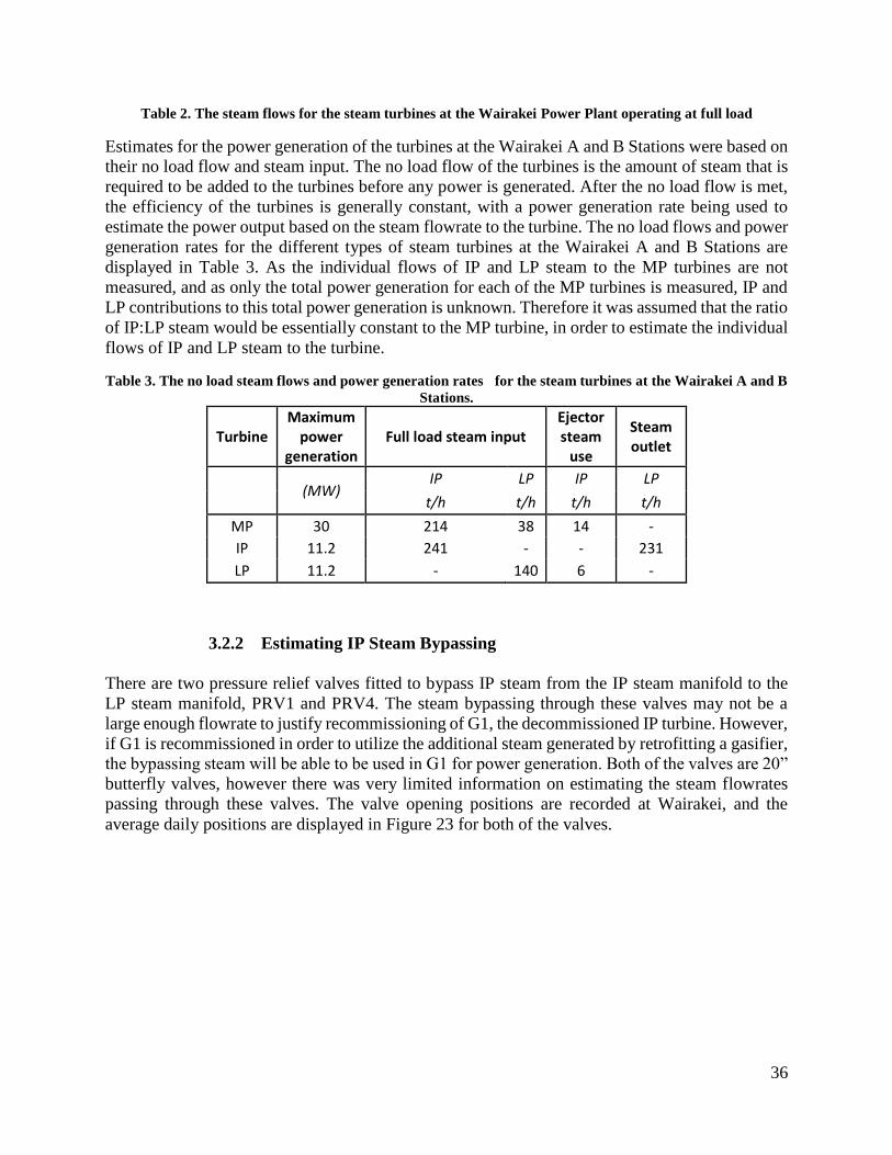
36
Table 2. The steam flows for the steam turbines at the Wairakei Power Plant operating at full load
Estimates for the power generation of the turbines at the Wairakei A and B Stations were based on
their no load flow and steam input. The no load flow of the turbines is the amount of steam that is
required to be added to the turbines before any power is generated. After the no load flow is met,
the efficiency of the turbines is generally constant, with a power generation rate being used to
estimate the power output based on the steam flowrate to the turbine. The no load flows and power
generation rates for the different types of steam turbines at the Wairakei A and B Stations are
displayed in Table 3. As the individual flows of IP and LP steam to the MP turbines are not
measured, and as only the total power generation for each of the MP turbines is measured, IP and
LP contributions to this total power generation is unknown. Therefore it was assumed that the ratio
of IP:LP steam would be essentially constant to the MP turbine, in order to estimate the individual
flows of IP and LP steam to the turbine.
Table 3. The no load steam flows and power generation rates for the steam turbines at the Wairakei A and B
Stations.
Turbine Maximum
power generation
Full load steam input Ejector steam
use
Steam outlet
(MW)
IP LP IP LP
t/h t/h t/h t/h
MP 30 214 38 14 -
IP 11.2 241 - - 231
LP 11.2 - 140 6 -
3.2.2 Estimating IP Steam Bypassing
There are two pressure relief valves fitted to bypass IP steam from the IP steam manifold to the
LP steam manifold, PRV1 and PRV4. The steam bypassing through these valves may not be a
large enough flowrate to justify recommissioning of G1, the decommissioned IP turbine. However,
if G1 is recommissioned in order to utilize the additional steam generated by retrofitting a gasifier,
the bypassing steam will be able to be used in G1 for power generation. Both of the valves are 20”
butterfly valves, however there was very limited information on estimating the steam flowrates
passing through these valves. The valve opening positions are recorded at Wairakei, and the
average daily positions are displayed in Figure 23 for both of the valves.

37
Figure 23. The daily average valve positions for two bypass valves, PRV1 and PRV4
In order to estimate the flowrate of steam through the valves, flow coefficients for 20” butterfly
valves were investigated from manufacturer’s information. It was found that the flow coefficient
for butterfly valves changes significantly by manufacturer and for different material specifications.
Due to this, there is a relatively large uncertainty attached to any estimations on steam flowrate
generated using these values. It was decided to use a conservative estimation for the flow
coefficients, in order to not overestimate the bypassing steam flowrate. The flow coefficients used
are displayed in Table 4.
Table 4. The assumed flow coefficients for 20" butterfly valves [50]
Valve Position (°) Flow Coefficient (CV)
30 2574
50 5720
70 10725
90 (full open) 14300
The flow could then be estimated using Equation 14, [51].
𝑾 = 𝟐. 𝟏𝑪𝑽√∆𝑷(𝑷𝟏 + 𝑷𝟐) (14)
Where:
W = the flowrate of saturated steam (lbs/h)
Cv = the valve flow coefficient
ΔP = the pressure drop across the valve (psi)
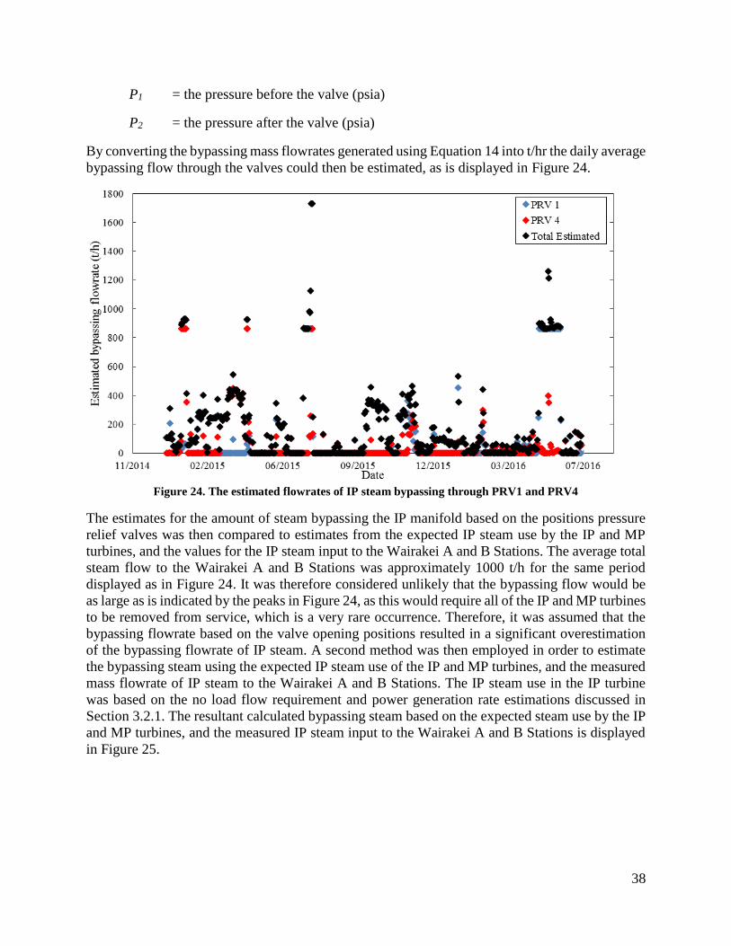
38
P1 = the pressure before the valve (psia)
P2 = the pressure after the valve (psia)
By converting the bypassing mass flowrates generated using Equation 14 into t/hr the daily average
bypassing flow through the valves could then be estimated, as is displayed in Figure 24.
Figure 24. The estimated flowrates of IP steam bypassing through PRV1 and PRV4
The estimates for the amount of steam bypassing the IP manifold based on the positions pressure
relief valves was then compared to estimates from the expected IP steam use by the IP and MP
turbines, and the values for the IP steam input to the Wairakei A and B Stations. The average total
steam flow to the Wairakei A and B Stations was approximately 1000 t/h for the same period
displayed as in Figure 24. It was therefore considered unlikely that the bypassing flow would be
as large as is indicated by the peaks in Figure 24, as this would require all of the IP and MP turbines
to be removed from service, which is a very rare occurrence. Therefore, it was assumed that the
bypassing flowrate based on the valve opening positions resulted in a significant overestimation
of the bypassing flowrate of IP steam. A second method was then employed in order to estimate
the bypassing steam using the expected IP steam use of the IP and MP turbines, and the measured
mass flowrate of IP steam to the Wairakei A and B Stations. The IP steam use in the IP turbine
was based on the no load flow requirement and power generation rate estimations discussed in
Section 3.2.1. The resultant calculated bypassing steam based on the expected steam use by the IP
and MP turbines, and the measured IP steam input to the Wairakei A and B Stations is displayed
in Figure 25.

39
Figure 25. The estimated bypassing steam calculated using IP steam flow estimates within and measured IP
steam input to the Wairakei A and B Stations
As can be seen in Figure 25, the estimates for the maximum amount of bypassing steam are much
more reasonable when based on the expected steam flowrates within the plant, compared to the
bypassing valve opening position. The trend of the decreasing amount of steam bypassing was
deemed to be sensible, as the flowrate of IP steam to the Wairakei A and B Stations has a
corresponding decrease across this period. A decreased amount of IP steam input would have a
reduction in the amount of bypassing steam, provided there was no change in the turbines that are
in operation. However, as there is an estimated uncertainty of ±10% on the flow measurements of
IP steam to the plant, and the steam use within the plant is based on “rules of thumb” about the
steam use of the different turbines, there is significant uncertainty on the estimated bypassing
steam. It is also noted, the estimates shown in Figure 25 indicate that bypassing occurs almost
constantly throughout the period. It was therefore decided that a technique using both the data for
the valve position and the estimates for the steam flow within the plant should be employed.
As the estimates for the amount of steam bypassing based on the valve positions was seen to be an
overestimation, it was decided that the estimates generated based on the expected steam use within
the plant would be more suitable. However, it was decided that it was likely that the information
on when the valves are fully closed could be used to estimate when no bypassing was occurring.
As bypassing only occurs sporadically within the plant, the estimates of near consistent bypassing
displayed in Figure 25 were deemed unlikely. Therefore, the minimum estimate on the amount of
bypassing steam generated by either of the methods was used in order to estimate the bypassing
steam. This ensured that the majority of the time there was essentially no steam bypassing, as
would be expected based on the positions of the control valves, and there was not the massive
estimations for bypassing steam that is observed when estimating bypassing steam based on the
valve positions. The amount of steam estimated to be bypassing using this method is displayed in
Figure 26.

40
Figure 26. The estimated bypassing steam based on both the estimated unused IP steam, and the pressure
relief valve positions
The estimated bypassing steam could then be added to any additional IP steam from the hybrid
configurations, in order to estimate the potential power generation in the IP turbines. However, as
there is some condensation of the steam in the IP turbines, there is consequently a slightly reduced
flowrate of the steam added to the LP manifold if it is utilized in the IP turbine instead of bypassing.
Similarly, the fact that there is IP steam bypassing into the LP manifold will reduce the power
losses from using IP steam as an input to the gasifier. In most of the potential hybrid configurations,
additional steam is being added to the IP manifold, so there is no decrease in power generation by
using this steam. However, as heating SGW for use in the binary plant does not produce IP steam,
there is a net decrease in the power generation at the Wairakei A and B Stations. If steam is
bypassing the IP turbines, the reduction of the IP steam to the Station will not necessarily reduce
the power generation from the IP turbines. Therefore, the expected power losses can be more
accurately estimated using the data for the expected steam bypassing the IP turbines.
3.2.3 Modelling Power Generation from Additional Steam Supply
As several of the hybrid configurations proposed generate additional power by increasing the
steam supply to the Wairakei Power Station, a method to estimate the power gains from the steam
was created. The gasifier is modelled to utilize geothermal IP steam, the potential power gains
must therefore be evaluated based on net steam generation, not the gross steam generation. Any
additional steam that may be generated at Wairakei would likely be utilized in IP and LP turbines
instead of MP turbines. This is due to the fact that there are unused IP and LP turbines that have
been removed from service at Wairakei, and one LP turbine is currently not fully loaded, as
displayed in Figure 27. The power generation expected from the turbines from the additional steam

41
was evaluated using the values for power generation after the no load flow has been met displayed
in Table 3.
Figure 27. The power generation from the three LP turbines at Wairakei
As can be seen in Figure 27, one of the LP turbines is generally unloaded, especially in 2016.It is
therefore valid to assume that one LP turbine is available for utilization without the associated
costs of bringing a turbine back into service. For simplicity it is assumed that G7 is unloaded, as it
can be seen that G7 is the turbine most consistently unutilized. Therefore, there is capacity for
approximately 140 t/h of LP steam to be used in G7, however, there is little to no capacity for IP
steam generation without bringing turbines back into service. There are currently two turbines that
are removed from service that may be returned to service, though this will require a workover and
recertification, the IP turbine G1, and the LP turbine G8. As approximately 95% of the steam input
to IP turbines is throttled down to LP, it is preferable to utilize the steam first in IP turbines, then
in the LP turbines. 6 t/h of IP steam is also required in order to operate the ejectors to operate each
LP turbine, and this must be factored in. As there is the no load flow requirement of 100 t/h for IP
turbines, if less than 106 t/h of IP steam is generated, there is no benefit in using the IP turbine at
all, and all of the steam should be passed through a pressure reducing valve and passed to the LP
manifold.
The power that may be generated from the additional steam was evaluated based on the steam that
can be generated. If less than 106 t/h of IP steam is available, including any estimated bypassing
steam, then there will be insufficient steam to utilize IP turbines. Thus, the steam will be throttled
down to LP, and be utilized in the LP turbines. By analysing the performance of the turbines, the
equations for power generation may be calculated. Also, as the maximum amount of IP steam that
can be utilized in IP turbines is approximately 241 t/h, any IP steam above this amount will be
bypassed to the LP manifold. Similarly, there is a maximum flowrate of approximately 140 t/h of
LP steam that can be used in each of the LP turbines. Therefore a flowrate of LP steam larger than

42
280 t/h will not generate any additional power from the LP turbines, as there is one unloaded LP
turbine (G7), and one LP turbine that may be returned to service (G8).
If steam available is > 106 t/h Equations 15-17 should be used:
𝑷𝑰𝑷 =(�̇�𝑰𝑷−(𝟏𝟎𝟎+𝟔𝒏𝑳𝑷))
𝟏𝟒 (15)
�̇�𝑳𝑷 =𝟐𝟑𝟏
𝟐𝟒𝟏�̇�𝑰𝑷 (16)
𝑷𝑳𝑷 =(�̇�𝑳𝑷−𝟏𝟗𝒏𝑰𝑷)
𝟏𝟏 (17)
However, if the IP steam available is not sufficient to meet the no load flow for the IP turbines,
then Equations 18-20 should be used:
𝑷𝑰𝑷 = 𝟎 (18)
�̇�𝑳𝑷 = �̇�𝑰𝑷 (19)
𝑷𝑳𝑷 =�̇�𝑳𝑷−𝟏𝟗𝒏𝑳𝑷
𝟏𝟏 (20)
Where:
PIP = the additional power generation from IP turbines (MW)
�̇�𝐼𝑃 = the net flowrate of IP steam available, maximum of 241, (t/h)
�̇�𝐿𝑃 = the net flowrate of LP steam available, maximum of 280, (t/h)
nLP = the number of LP turbines that may be operated with the steam generated
PLP = the additional power generation from LP turbines (MW)
The overall additional power generation is the sum of the power generation from the IP and LP
turbines. If less than 13 t/h of steam is available for use, no power will be generated in the IP
turbines or LP turbines, as the no load flow will not be able to be met for either the IP or the LP
turbines.
3.2.4 Decreasing Steam Supply to the Wairakei A and B Stations
There are steam extraction limits on the amount of the two-phase fluid that may be extracted at the
Wairakei Geothermal Field. The amount of two-phase fluid is therefore expected to remain
relatively constant. However the average enthalpy of the extracted two-phase fluid is decreasing,
and therefore there is a corresponding decrease in the mass flowrate of the steam generated. While
the total mass flowrate decrease is relatively small, the Wairakei A and B Stations observe
significant reductions in the mass flowrate of input steam. As IP steam is preferentially used at the
Te Mihi and Poihipi Rd Power Stations, the reduction of mass flowrate is compounded for the

43
Wairakei A and B Stations. The IP steam flowrate to the Wairakei A and B Stations, and the
estimated bypassing flowrate is displayed in Figure 28. Due to the decreasing steam flowrate,
much of the analysis of the bypassing steam at the Wairakei A and B Stations will likely not be
representative of future bypassing steam flowrates. Consequently, analysis performed on the
power generation that may be possible using the bypassing steam if utilized in a recertified IP
turbine will overestimate the power generation that may be possible. Therefore, three scenarios
were created in order to represent different possibilities for the amount of steam passing to
Wairakei:
Bypassing, G4 fully loaded
This is the case for the most of 2015, where there is some bypassing, and G4 is almost
continuously fully loaded. In this case, an IP turbine would need to be brought back into service
in order to utilize additional IP steam. The bypassing steam would also be able to be used to
generate power from the recertified IP turbine.
No bypassing, G4 fully loaded
As can be seen in Figure 27, the amount of steam bypassing has been decreasing consistently
throughout 2015 and into 2016, there is almost no steam bypassing for the majority of 2016.
If it is assumed that the amount of steam input to Wairakei is at a point where no bypassing
occurs, but the IP and MP turbines are fully loaded, then additional power generation would
be hindered. This is due to the fact that any steam generated would need to surpass the no load
flow of the IP turbines of approximately 100 t/h in order to generate any power from the IP
turbines, and the steam generated is not augmented by any bypassing steam.
No bypassing, G4 and G9 not fully loaded
If the steam supply to the Wairakei A and B Stations drops even further, then this will cause
the IP turbine G4 to not be fully loaded. Due to this, any IP steam generated may be used in
G4. This will result in increased power generation, as the no load flow for G4 may be met by
the existing IP steam supply. Similarly, the no load flow for G9 is assumed to be met by the
existing geothermal LP steam, and therefore additional LP steam may be use to directly
generate power.

44
Figure 28. The total steam input to the Wairakei A and B Stations, and the estimated bypassing steam
The decision was made to create the three cases for steam input to Wairakei instead of
extrapolating steam data to estimate the future steam flowrates, due to the many factors involved
with the future steam flowrates. One of the factors of concern was the fact that the Te Mihi Power
Plant is limited by the amount of SGW it can reinject. Therefore as the average enthalpy of the
two-phase fluid decreases, relatively more SGW will be generated for the same steam flowrate.
There is a pipeline that is currently being used to provide the Wairakei A and B Stations with steam
which can instead be used as a SGW reinjection line for Te Mihi if need be. Therefore there would
be a significant step reduction in the steam supply to Wairakei, if the average enthalpy of the
reservoir decreases to the point where the existing SGW reinjection infrastructure for Te Mihi
becomes undersized.
3.3 Modelling the Hybrid Configurations
Once models for biomass gasification, and the Wairakei steam manifold and steam turbines were
created, the modifications required to implement the hybrid configurations could be modelled
using UniSim. The syngas created in the gasifier model was then combusted using a conversion
reactor function, and the heat generated from this combustion could be used in the different hybrid
configurations.
3.3.1 Superheating of Geothermal Steam
In order to evaluate the effect of superheating the geothermal steam would have on the power
generation, and steam use in the plant, the gasification and Wairakei Power Station UniSim models

45
were combined, and a syngas fired steam superheater was added to the combined model. A
conversion reactor was used to model the combustion of the syngas, an 80% heat transfer
efficiency was used for the energy transferred from the syngas combustor and the steam
superheater. It was assumed that this heat transfer efficiency could be calculated in the same
manner as for a boiler. This heat transfer efficiency was then estimated using the hydrogen:carbon
ratio of the fuel [52] [53]. A 10% oxygen excess was used to calculate the air requirement to the
superheater [40]. A flue gas outlet temperature of 200°C from the furnace was assumed in order
to estimate the heat transfer to the IP steam, and estimate the amount recycled syngas required in
order to adequately dry the wood chips in the rotary dryer. It was also assumed that the adiabatic
efficiency of the turbine would remain unchanged after the turbine was modified to operate using
superheated steam.
As the superheated steam generated in this case would have to be utilized in the existing Wairakei
turbines, the design constraints of this limited how the turbine would likely be able to be used. The
design conditions for the modified turbines were largely based on those suggested in a report by
Morris investigating superheating geothermal steam for use in existing steam turbines [38]. Due
to the fact that the steam turbines would likely not be able to safely use steam that had a much
higher pressure than the turbines were designed for, the maximum pressure of the superheated
steam was set as the same as the IP steam at 4.5 bara. The amount of superheating that could be
performed on the geothermal steam was then limited by the maximum temperature the steam could
be heated to. It was decided that this maximum temperature would be limited by the creep range
of the low alloy steel used in the plant, at 370°C [54], a safety margin of 20°C was then imposed,
changing the maximum operational superheated steam temperature to 350°C. The volumetric
flowrate of the superheated steam would also have to be designed to be approximately the same as
in the non-superheated case, in order to not damage the turbines. As the volumetric flowrate is to
be held constant, the allowable mass flowrate in the superheated case would be lower than in the
saturated case, due to the decreased density of superheated steam. The power able to be generated
by the steam turbine can be found using Equation 1:
�̇�𝑺𝑻 = �̇�𝑺(𝒉𝒊𝒏 − 𝒉𝒐𝒖𝒕) (1)
The power generated by the superheated steam is reduced due to this decrease in the mass flowrate,
and may even be less than in the saturated steam case, depending on the enthalpy drop that can be
achieved within the turbine. As the volumetric flowrate is being held constant for both the
superheated and saturated steam cases, the mass flowrate can be determined using the ratio of the
density of the saturated steam and the superheated steam. The density of the saturated steam at
150°C and 4.5 bara was found to be 2.416 kg/m3, and the density of the superheated steam at
350°C and 4.5 bara found at 1.577kg/m3, leading to an allowable mass flowrate of superheated
steam to be 65.3% of that of the saturated steam. The MP turbines operate in two stages, the first
stage brings the IP steam down to LP, and the second stage expands this LP steam and additional
LP steam that is injected to the turbine after the first stage to the vacuum conditions. By introducing
superheated steam to the MP turbine, the mass flowrate of steam introduced to the first stage is
decreased by approximately 35%, but the amount of additional LP steam injected to the MP turbine
is increased by 34%. This is due to the relatively lower volumetric flowrate of steam exiting the
first stage when superheated steam is used compared to the saturated case, this then requires a
larger amount of additional LP steam to be added before the second stage.
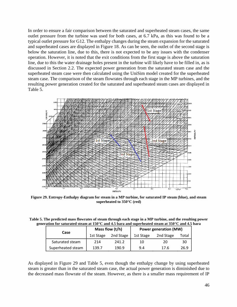
46
In order to ensure a fair comparison between the saturated and superheated steam cases, the same
outlet pressure from the turbine was used for both cases, at 6.7 kPa, as this was found to be a
typical outlet pressure for G12. The enthalpy changes during the steam expansion for the saturated
and superheated cases are displayed in Figure 18. As can be seen, the outlet of the second stage is
below the saturation line, due to this, there is not expected to be any issues with the condenser
operation. However, it is noted that the exit conditions from the first stage is above the saturation
line, due to this the water drainage holes present in the turbine will likely have to be filled in, as is
discussed in Section 2.2. The expected power generation from the saturated steam case and the
superheated steam case were then calculated using the UniSim model created for the superheated
steam case. The comparison of the steam flowrates through each stage in the MP turbines, and the
resulting power generation created for the saturated and superheated steam cases are displayed in
Table 5.
Figure 29. Entropy-Enthalpy diagram for steam in a MP turbine, for saturated IP steam (blue), and steam
superheated to 350°C (red)
Table 5. The predicted mass flowrates of steam through each stage in a MP turbine, and the resulting power
generation for saturated steam at 150°C and 4.5 bara and superheated steam at 350°C and 4.5 bara
Case Mass flow (t/h) Power generation (MW)
1st Stage 2nd Stage 1st Stage 2nd Stage Total
Saturated steam 214 241.2 10 20 30
Superheated steam 139.7 190.9 9.4 17.6 26.9
As displayed in Figure 29 and Table 5, even though the enthalpy change by using superheated
steam is greater than in the saturated steam case, the actual power generation is diminished due to
the decreased mass flowrate of the steam. However, as there is a smaller mass requirement of IP

47
steam for the turbine, there is the potential of utilizing the unused steam in other turbines in order
to generate additional power. The method described in Section 3.2.3 could then be used to evaluate
the additional power generation that may be possible from the saved steam.
3.3.2 Vaporization of Steam Turbine Condensate
In order to evaluate the additional power that could be generated from the vaporized steam
condensate, a model for a boiler was created in UniSim. By investigating the heat transfer
efficiencies of boilers, it was found that by using the hydrogen:carbon ratio of the syngas and the
flue gas outlet temperature of the syngas as indicators, an 80% heat transfer efficiency could be
used for the boiler including the stack losses, and the convection and radiation losses[52] [53]. A
10% air excess was used to calculate the air requirement to the boiler [40]. The flue gas produced
by the boiler was used to aid in the drying of the wet biomass to the gasifier, by being used as the
drying medium in the rotary drum dryer. A conversion reactor was used in order to model the
syngas combustion, and 80% of the heat removed from the reactor was added to the condensate
using a heat exchanger. A separator was used in order to model the blowdown of the boiler, the
blowdown required by the boiler water chemistry could be input, and the resulting steam
generation determined.
In order to increase the amount of additional steam that may be generated, a preheater for the
condensate was employed. The temperature of the SGW would depend on the source of the
condensate, as the SGW resource would likely be that located in close proximity to condensate to
minimize the length of pipelines required. It was assumed that the condensate could be heated to
100°C prior to being introduced into the boiler, as the majority of SGW available is at a higher
temperature than this. The outlet temperature of the SGW from the preheater was set as 90°C, as
temperatures lower than this may increase the rate of silica precipitation in the heat exchanger
[24].
The deaeration of the boiler feed water was then modelled to be performed by further heating the
condensate to 103°C using a recycle stream from the steam produced in the boiler. The amount of
steam vented in the deaerator was calculated by setting a vent rate of the recycled steam. A
controller was used to adjust the amount of recycled steam in order to achieve the desired rate of
venting.
The blowdown of the boiler could be set in the UniSim model, to that required based on the boiler
water purity. The flowrate of the condensate is then automatically calculated, based on the heat
transfer from syngas combustion, the quality of the steam from the boiler, and the boiler
blowdown.
As the pressure of the condensate is initially at 7.8 kPaa, pumping needs to be performed before
the condensate can be fed to the boiler. As the deaerator operates at approximately 115 kPaa, and
the boiler operates at 450 kPaa, two stages of pumping were required for the boiler operation, prior
to the preheater, and again after the deaeration stage.

48
3.3.3 Heating the Separated Geothermal Water after the First Separation
Stage
In order to estimate the amount of additional steam that may be produced by performing heating
on the SGW after the first separation stage, a UniSim model was created. The design of the model
was very similar to the model created for the turbine condensate boiler described in Section 2.2.4.
An 80% efficiency for the heat transfer to the boiler from syngas combustion was assumed, and a
10% oxygen excess used for the air flowrate to the boiler. It was assumed that heat loss between
the first separation stage and the boiler would be negligible, and the temperature of the condensate
was found from the saturated steam conditions from the first separation stage.
The reduction of metals being disposed of into the Waikato River was also estimated. As the
solubility of metals is much higher in liquid water than in steam, it was assumed that all of the
metals in the two-phase fluid are present in the SGW. For simplicity, the water streams have been
assigned numbers, as displayed in Figure 30.
FP14IP
FP14ILP
Boiler
1
2
4
5
3
6 7
8
9
1011
12
13
14
Drain
Figure 30. Numbered streams of steam and SGW around the modified FP14
The flowrates for ILP steam (Stream 9), the reinjection in X-line (Stream 11), and the reinjection
in T-line (Stream 14) will be relatively constant. Therefore, the flowrate IP SGW to the drain
(Stream 13) and the IP steam generated (Stream 3) will be the only exiting streams to have a mass
flowrate change with changing IP steam generation in the boiler (Stream 5). The following mass
balance was then performed in order estimate the potential decrease in metal flowrate to the
Waikato River, where:
�̇�𝑚,𝑥 = the mass flowrate of the metal of interest in Stream x (g/h)
�̇�𝑤,𝑥 = the mass flowrate of water (liquid or gas) in Stream x (t/h)

49
𝐶𝑚,𝑥 = the concentration of the metal of interest in Stream x (g/t)
The mass flowrate of metals draining to the Waikato River is the sum of those from Stream 12 and
Stream 13, and can be calculated from Equation 21.
�̇�𝒎,𝑫𝒓𝒂𝒊𝒏 = �̇�𝒎,𝟏𝟐 + �̇�𝒎,𝟏𝟑 = �̇�𝒘,𝟏𝟐𝑪𝒎,𝟏𝟐 + �̇�𝒘,𝟏𝟑𝑪𝒎,𝟏𝟑 (21)
As it is assumed no metals leave in the steam in Streams 2, 5, and 9; Equation 22 can be created.
�̇�𝒎,𝟏 = �̇�𝒎,𝟒 = �̇�𝒎,𝟔 (22)
The mass flowrate of metals draining into the Waikato from Stream 13 can be found using
Equations 23 –26
𝑪𝒎,𝟔 = 𝑪𝒎,𝟕 = 𝑪𝒎,𝟖 = 𝑪𝒎,𝟏𝟑 = 𝑪𝒎,𝟏𝟒 (23)
�̇�𝒘,𝟏𝟑=�̇�𝒘,𝟏 − �̇�𝒘,𝟐 − �̇�𝒘,𝟓 − �̇�𝒘,𝟕 − �̇�𝒘,𝟏𝟒 (24)
𝑪𝒎,𝟔 =�̇�𝒘,𝟏
�̇�𝒘,𝟏−�̇�𝒘,𝟐−�̇�𝒘,𝟓𝑪𝒎,𝟏 = 𝑪𝒎,𝟏𝟑 (25)
�̇�𝒎,𝟏𝟑 = �̇�𝒘,𝟏𝟑𝑪𝒎,𝟏𝟑 (26)
The mass flowrate of metals draining into the Waikato from Stream 12 can be found using
Equations 27 –29
𝑪𝒎,𝟏𝟎 = 𝑪𝒎,𝟏𝟏 = 𝑪𝒎,𝟏𝟐 (27)
𝑪𝒎,𝟏𝟎 = (�̇�𝒘,𝟕
�̇�𝒘,𝟕−�̇�𝒘,𝟗) (
�̇�𝒘,𝟏
�̇�𝒘,𝟏−�̇�𝒘,𝟐−�̇�𝒘,𝟓) 𝑪𝒎,𝟏 = 𝑪𝒎,𝟏𝟐 (28)
�̇�𝒎,𝟏𝟐 = �̇�𝒘,𝟏𝟐𝑪𝒎,𝟏𝟐 (29)
As the mass flowrate of Stream 12 will remain relatively constant with the amount of additional
steam generated in the boiler, the total mass flowrate of metals entering the Waikato may then be
calculated. Using the average flowrates for the streams around FP14 for 2015, it was found that
the decrease of metal flowrate could be estimated for the amount of additional steam using
Equation 30.
�̇�𝒎,%𝒅𝒆𝒄𝒓𝒆𝒂𝒔𝒆 = 𝟓. 𝟗𝟕 × 𝟏𝟎−𝟕�̇�𝒘,𝟓𝟐 + 𝟓. 𝟕𝟔 × 𝟏𝟎−𝟒�̇�𝒘,𝟓 (30)
Where:
�̇�𝑚,%𝑑𝑒𝑐𝑟𝑒𝑎𝑠𝑒 = the decrease in the flowrate of metals entering the Waikato River from FP14 (%)
3.3.4 Heating Additional Separated Geothermal Water for use in a Binary
Plant

50
As the binary plant at Wairakei has been in service since 2009, there are existing correlations used
in order to estimate the effect that a change in temperature of the SGW has on the power output of
the binary plant. By using a UniSim model to estimate the amount of heating that may be
performed on the SGW by a syngas fired heater, the associated power output could be determined.
The correction factor for temperature variation of the SGW influent to the binary plant is given by
Equation 31 and Equation 32 for different inlet temperatures.
For 120°C < T < 127°C the correction curve the correction curve is linear:
𝑭𝑻 = −𝟑. 𝟕𝟎 + 𝟎. 𝟎𝟑𝟗𝑻 (31)
For 127°C < T < 135°C the correction curve is a 4th order polynomial:
𝑭𝑻 = 𝒂 + 𝒃𝑻 + 𝒄𝑻𝟐 + 𝒅𝑻𝟑 + 𝒆𝑻𝟒 (32)
Where:
FT = the power output correction factor for changes of inlet SGW temperature
T = the temperature of the SGW entering the binary plant
The values of the constants in Equation 32 are:
a = -6231
b = 192
c = -2.22
d = 0.0114
e = -0.000022
By plotting the correction factor against the inlet temperature of the SGW, as displayed in Figure
31, it can be seen that the benefits diminish after heating the SGW above the design temperature
of 127°C. As the average temperature of the SGW entering the binary plant is 130°C, there are
limited benefits to further heating the inlet SGW away from the designed inlet temperature.
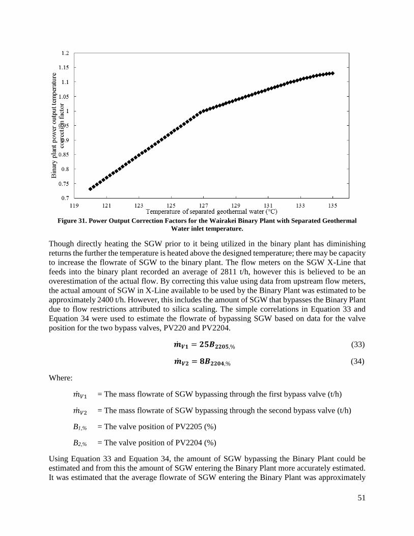
51
Figure 31. Power Output Correction Factors for the Wairakei Binary Plant with Separated Geothermal
Water inlet temperature.
Though directly heating the SGW prior to it being utilized in the binary plant has diminishing
returns the further the temperature is heated above the designed temperature; there may be capacity
to increase the flowrate of SGW to the binary plant. The flow meters on the SGW X-Line that
feeds into the binary plant recorded an average of 2811 t/h, however this is believed to be an
overestimation of the actual flow. By correcting this value using data from upstream flow meters,
the actual amount of SGW in X-Line available to be used by the Binary Plant was estimated to be
approximately 2400 t/h. However, this includes the amount of SGW that bypasses the Binary Plant
due to flow restrictions attributed to silica scaling. The simple correlations in Equation 33 and
Equation 34 were used to estimate the flowrate of bypassing SGW based on data for the valve
position for the two bypass valves, PV220 and PV2204.
�̇�𝑽𝟏 = 𝟐𝟓𝑩𝟐𝟐𝟎𝟓,% (33)
�̇�𝑽𝟐 = 𝟖𝑩𝟐𝟐𝟎𝟒,% (34)
Where:
�̇�𝑉1 = The mass flowrate of SGW bypassing through the first bypass valve (t/h)
�̇�𝑉2 = The mass flowrate of SGW bypassing through the second bypass valve (t/h)
B1,% = The valve position of PV2205 (%)
B2,% = The valve position of PV2204 (%)
Using Equation 33 and Equation 34, the amount of SGW bypassing the Binary Plant could be
estimated and from this the amount of SGW entering the Binary Plant more accurately estimated.
It was estimated that the average flowrate of SGW entering the Binary Plant was approximately

52
2300 t/h for 2015. The flowrate of SGW entering the Binary Plant, bypassing the Binary Plant,
and the designed flowrate of SGW for the Binary Plant are displayed in Figure 32.
Figure 32. The mass flowrate of SGW feed to the Wairakei Binary Plant, and the estimated amount of SGW
bypassing the Binary Plant.
The additional power generation that will result from increasing the mass flowrate of SGW to the
binary plant is estimated using Equation 35 and Equation 36.
For SGW flow 50% of design ≤ �̇�%𝑂𝐷≤ 100% of design:
𝑭�̇� = −𝟎. 𝟒𝟐𝟖𝟖 + 𝟎. 𝟎𝟏𝟒𝟐𝟖𝟖�̇�%𝑶𝑫 (35)
For SGW flow 100% of design ≤ �̇�%𝑂𝐷 ≤ 114.3% of design:
𝑭�̇� = 𝟎. 𝟖𝟑𝟗𝟎𝟒𝟖𝟐𝟗 + 𝟎. 𝟎𝟎𝟏𝟔𝟎𝟗𝟓𝟕𝟏�̇�%𝑶𝑫 (36)
Where:
𝐹�̇� = The power output correction factor for changes of inlet SGW flowrate
�̇�%𝑂𝐷 = The mass flowrate of the SGW entering the binary plant as a % of the designed
flowrate
Using Equation 35 and Equation 36, the effect of increasing the flowrate of SGW to the binary
plant can be estimated, as is displayed in Figure 33. As can be seen, the benefits of increasing the
flowrate of SGW to the binary plant sharply diminish once increased above the design flowrate.

53
Figure 33. Power output correction factors for the Wairakei Binary Plant with separated geothermal water
flowrate to the Binary Plant.
Historical data for the flowrate and temperature was used with the correction factors to estimate
the amount of additional power that may be generated using a syngas fired heat exchanger to heat
T-Line and augment the amount of SGW being fed to the Binary Plant. It was assumed that the
maximum flowrate that the Binary Plant could utilize is 3200 t/h, given by the upper bound of
Equation 36 at 114.3% of the design flowrate of 2800 t/h. It was found that the most effective use
of the syngas fired heating was to heat the SGW in T-Line as little as possible, as the added power
generation from increasing the temperature of the SGW did not meet the costs for the landing
residues required. The heated temperature of the SGW taken from T-Line was therefore set to be
equal to the temperature of the SGW in X-Line. It was also found that the benefits to power
generation from increasing the total flowrate to the Binary Plant to higher than the designed
flowrate was also offset by the cost of the landing residues required. The amount of T-Line that is
to be heated and added to X-Line, and the resulting total mass flowrate of SGW to the Binary Plant
are displayed in Figure 34.
As it was determined to heat only the amount of T-Line to satisfy the design flowrate, where
possible, and to only heat T-Line to the same temperature as X-Line; there is a relatively small
amount of heating required to be performed by the syngas. The amount of heat that was required
to be provided by the syngas combustion to achieve the additional power generation displayed in
Figure 26 and the corresponding landing residues requirement were calculated and are displayed
in Figure 36.

54
Figure 34. The additional SGW from T-Line that may be added to the feed of the Binary Plant and the
resultant total SGW flowrate
As can be seen in Figure 34, the SGW in T-Line is only added when the flowrate of X-line is less
than the designed flowrate of 2800 t/h. When the combined flow of T-Line and X-Line would be
greater than the designed flowrate, only enough of T-Line was added in order to reach the designed
flowrate, as exhibited by the plateau in the second half of 2015.
The power generation of the Binary Plant for 2015 and the estimated power generation with the
heating and additional SGW from T-Line is displayed in Figure 35. It is estimated that the power
generation of the Binary Plant will increase on average from 13.5 MW to 15.3 MW from the
additional SGW. However, there will also be a decrease in the power generation at the Wairakei
A and B Stations due to the use of IP steam in the gasifier.

55
Figure 35. The Power Generation of the Wairakei Binary Plant for 2015 and the estimated power generation
by heating and adding additional SGW from T-Line
Figure 36. The heat requirement and associated biomass input in order to heat additional SGW in T-line
56
3.4 Energy Efficiency
The power generation and the efficiency of power generation from the biomass input were used as
a basis, in order to compare the four proposed hybrid geothermal/gasification configurations. The
amount of energy present in the biomass feed to the gasifier was calculated using a value for the
net calorific value of 19.2 MJ/kg oven dried wood [55]. As a moisture content of 50% (wet basis)
was assumed, the net calorific of 9.6 MJ/kg wet wood was used to calculate the energy input from
the woody biomass feed. Once the additional power generation was calculated, the electrical
energy efficiency could be calculated using Equation 37.
𝜼 =𝑷𝒐𝒖𝒕𝒑𝒖𝒕
𝑷𝒊𝒏𝒑𝒖𝒕 (37)
Where:
η = the electrical energy efficiency
Poutput = the additional electrical power output from the hybrid configuration
(MW)
Pinput = the power input of the biomass feed based on its calorific value (MW)
The efficiencies of the different configurations are expected to be highly variable with the size of
the hybrid configurations, as factors such as the no load flow of the turbines do not scale with the
size of the hybrid configurations. As the no load flow of the turbines becomes relatively less
influential on the potential power generation from creating additional IP steam, it is expected that
in general the larger the hybrid configuration is, the greater the energy efficiency. However, it is
also noted, that the most economical sized hybrid configuration will likely not be the most energy
efficient, due to the increasing cost of landing residues with increasing residue input. Though the
hybridized Binary Plant configuration would not produce additional steam, the average energy
efficiency of the plant will still be affected, if a limit is placed on maximum amount of landing
residues. The efficiency of the plant will also be highly variable for all of the hybrid configurations,
depending on the amount of steam which would otherwise bypass the IP turbines at Wairakei,
without these turbines being returned to service, therefore a yearly average for the expected hybrid
plant efficiencies will be used for comparison.

57
4.0 Determining the Suitability of Geothermal Waters to be used
as Boiler Feed Water
There are strict tolerances on the allowable concentrations of contaminants in boiler feed water, in
order to ensure stable and safe operation of the boiler. As the condensate vaporization hybrid
configuration described in Section 2.2.4 uses geothermal steam condensate as boiler feed water; it
is necessary to perform testing on samples of geothermal condensate in order to determine if the
condensate can be used directly as boiler feed water, or failing this a water treatment process stage
introduced.
4.1 Boiler Feed Water Tolerances
In order to evaluate the relative quality of the geothermal steam condensate, the tolerances for
contaminants in boiler feed water were investigated. The tolerances for the boiler feed water were
found to be strongly pressure dependent, with the allowable contaminant concentrations
decreasing as boiler pressure increases. The American Society of Mechanical Engineers (ASME)
has guidelines for boiler feed water and boiler water purity for some contaminants, as displayed in
Table 6 and Table 7 respectively[40]. As the condensate boiler would likely be designed to
generate steam which may be added directly to the IP steam manifold at the Wairakei Steam Field,
the boiler would likely operate at 4.5 bara. As can be seen in Table 6 and Table 7, the relatively
low boiler drum pressure required to produce the 4.5 bara steam has less stringent steam purity
requirements than for higher pressure boilers.
Table 6. ASME guidelines for feed water quality in modern industrial water tube boilers for reliable
continuous operation [40]
Drum pressure
Iron Copper pH Oxygen Total
hardness
(bar) (ppm Fe)
(ppm Cu) pH units (mg/L) (ppm CaCO3)
0 - 20.7 0.1 0.05 8-9.5 0.007 0.3
20.7 - 31.0 0.05 0.025 8-9.5 0.007 0.3
31.0 - 41.4 0.03 0.02 8-9.5 0.007 0.2
41.4 - 51.7 0.025 0.02 8-9.5 0.007 0.2
51.7 - 62.0 0.02 0.015 8-9.5 0.007 0.1
62.0 - 69.0 0.02 0.015 8-9.5 0.007 0.05
69.0 - 103.5 0.01 0.01 8.5-9.5 0.007 0
103.5 – 138.0 0.01 0.01 8.5 - 9.21 9.3 - 9.52
0.007 0
Note 1: with copper alloys in feed water heaters, Note 2: With carbon steel feed water heaters

58
Table 7. ASME guidelines for boiler water quality in modern industrial water tube boilers for reliable
continuous operation [40]
Drum pressure
Silica Total
alkalinity
Total Dissolved
Solids
Specific conductance
(bar) (ppm SiO2) (ppm CaCO3) (ppm) (µS/cm)
(un-neutralized)
0 - 20.7 150 700 700-3500 7000
20.7 - 31.0 90 600 600-3000 6000
31.0 - 41.4 40 500 500-2500 5000
41.4 - 51.7 30 400 400-2000 4000
51.7 - 62.0 20 300 300-1500 3000
62.0 - 69.0 8 200 250-1250 2000
69.0 - 103.5 2 0 100 150
103.5 – 124.0 1 0 100 100
124.0 – 138.0 1 0 50 100
Generally manufacturers and utility owners recommend that steam should have a silica content
between 10 and 20 ppb in order for silica scaling to not occur in steam turbines [40]. A second,
more conservative estimate for the permissible amount of silica in the boiler water was found to
be between 30-60 ppm, using Figure 37. In order to ensure that damage does not occur to the boiler
or to the steam turbines, the conservative estimate of 30 ppm silica in the boiler water was used as
the allowable amount of silica in the boiler water.
Figure 37. The permissible amount of silica in the boiler water in order to produce steam with a silica content
of 10 and 20 ppb [40].

59
After consulting a geothermal water engineer about the contaminants that should be tested for in
order for geothermal condensate to be used as boiler feed water, tests on the following were
decided to be performed [56]:
Conductivity
pH
SiO2
H2S
CO2
NH4
Chlorides
Na
Ca
Mg
Sulphates
The concentration of silica, sodium, calcium, and magnesium in the condensate are of interest, as
they may cause mineral deposition in a boiler or steam turbine if they are present in high enough
concentrations in boiler feed water [57]. Also, the hydrogen sulphide, chlorides, sulphates, and
carbon dioxide can cause corrosion within the boiler or turbine if present in the boiler feed water.
4.2 Water Available on Site
There are several sources of water available on the Wairakei Steam Field apart from the SGW.
These are the blowdown from the Wairakei A and B Power Stations, and Te Mihi Power station,
and also the condensate from the Poihipi Rd Power Station. The blowdown at the Wairakei A and
B, and the Te Mihi Power Stations is created in direct contact condensers using cooling water to
stimulate the condensation of the geothermal steam at the back end of the turbines. The condensate
generated in the direct contact condensers is cooled in a cooling tower, then a portion of the cooled
blowdown is reused as cooling water in the direct contact condensers. However, the Poihipi Rd
Power Station uses a shell and tube condenser and due to this, the condensate does not come into
contact with open air, and therefore the chance of contamination or gas absorption reducing the
purity of the condensate is removed.
It was decided to perform testing on three sources of water: the condensate from the Poihipi Rd
Power Station, the blowdown from Te Mihi, and the Blowdown from Ohaaki. The condensate
from the Wairakei A and B stations was not tested, as it was decided due to the fact that the direct
contact condensers using the Waikato River water as a cooling fluid would decrease the purity of
the resultant condensate, rendering it unsuitable as boiler feed water. The condensate from Poihipi
Rd was selected due to the fact that it is the only source of condensate generated in a shell and tube
condenser. The blowdown at Ohaaki and Te Mihi were selected in order to evaluate the purity of
blowdown generated in direct contact condensers using recycled blowdown as the cooling water.

60
4.3 Factors Affecting Water Purity
There are several factors that can influence the concentration of contaminants in the geothermal
condensate. Most of these factors relate to the amount of liquid geothermal water present that is
entrained into the steam turbines. This is due to the fact that the dissolved minerals in the
geothermal fluid have a much higher solubility in liquid water than in steam. Because of this, the
majority of the minerals present in the geothermal condensate are present due to entrained liquid
water. It is also known that minerals can be soluble in steam, however, within the range of steam
pressures generated at Wairakei, the solubility of minerals in steam is negligible compared to the
solubility in liquid water [58],[59]. Because of this, if liquid carryover in the steam increases, more
water treatment may be required for the condensate or blowdown to be used as boiler feed water.
Due to the higher mineral solubility in liquid water than in steam, the performance of the flash
plants separating the liquid and gasses greatly impacts the condensate and blowdown purity.
However, monitoring the performance of the flash plants at Wairakei during operation is difficult,
and no continuous monitoring of flash plant performance is conducted. Currently testing of the
performance of Flash Plant 15 and Flash Plant 16 are being conducted at Wairakei, in order to
address silica scaling problems at the Te Mihi Power Station. Specifically it is of interest to
discover the effect that the load on the flash plants and the separation pressure have on liquid carry
over. This is performed by injecting tracers into the two-phase fluid prior to the separators and
sampling the liquid removed from drain pots downstream. If the results from this flash plant
analysis indicate significant variability in flash plant performance, then efforts should be made to
evaluate the effect this will have on condensate and blowdown purity.
There are relatively long steam lines at the Wairakei Geothermal Field compared to other
geothermal power plants, and consequently there are both relatively high pressure and heat losses
from transportation at Wairakei. However, this causes a phenomenon called “passive scrubbing”
at Wairakei, where a large portion of the liquid carryover in the steam is deposited on the walls of
the pipelines, and subsequently removed in drain pots. This removal of liquid also serves to remove
a large amount of the minerals present in the steam.
Currently there are drain pots installed throughout the Wairakei Geothermal Field, in order to
remove condensate and liquid carryover in the steam lines. There are also demisters installed at
the Te Mihi, and Poihipi Rd Power Plants, in order to scrub any remaining liquid from the steam
prior to it being used in the turbines. However, it is believed that the demister at Poihipi Rd is
essentially out of operation, due to massive corrosion within it.
The steam wells used to extract the steam are also expected to have a large effect on the resulting
condensate and blowdown purity. The pressure and quality of the steam varies depending on the
wells used, with some wells at Wairakei even being considered “dry” as they have very low
moisture content. The geology at the different steam wells will affect the mineral content in the
fluid extracted from the wells, due to the differing mineral compositions of different rock
formations.
The oxygen content of the condensate and blowdown will be affected by the exposure of the water
to air. Dissolved oxygen must be maintained below a certain concentration in boiler feed water in
order to prevent corrosion or pitting in the boiler. The solubility of oxygen in water increases as

61
pressure increases and as temperature decreases, and the Poihipi Rd condensate is formed from the
condensation of geothermal steam under vacuum conditions at approximately 75 mbara and 40°C.
Because of this, the Poihipi Rd condensate is expected to have a much lower dissolved oxygen
content than the Te Mihi blowdown and Ohaaki blowdown as they are at atmospheric pressure.
Provided that there is no exposure of the Poihipi Rd condensate to oxygen, the condensate should
retain its low oxygen content even after its pressure is increased by pumping the condensate for
use in the boiler.
4.4 Sampling and Testing Procedure
The sampling and testing of the condensate and blowdown sources were designed with reference
to the Standard Methods For the Examination of Water and Waste water by the American Public
Health Association (APHA) [60]. As the testing for metals required nitric acid preservation on the
sample bottle, two separate samples were required to be taken for each source of water. 100 ml of
sample was taken in a sample bottle that was treated with nitric acid, along with 2L of raw sample.
The testing procedure for each of the contaminants of interest, and the detection limits of each test
is displayed in
Table 8.
The dissolved oxygen was tested on site, using a YSI Digital Model 58 Dissolved Oxygen Meter.
As the Poihipi Rd sample was the only sample that was not exposed to the open air, and had to be
extracted from pipelines, it was desired to minimize the contact with the air, as this would likely
result in an inaccurately high oxygen content in the sample. In order to minimize the oxygen
contamination, an apparatus was used to minimize contact the sample has with the air, as displayed
in Figure 38. A tube was used to inject the condensate directly from the sampling point into the
sampling container. The design of the sampling container ensured that the condensate did not come
into contact with air, however as there was not a perfect seal between the oxygen meter probe and
the sampling container, there may be been some contact with the air.
Dissolved oxygen meterDissolved oxygen meter
Oxygen meter probe
Condensate sampling point
Sample
Sampling container
Tubing
Figure 38. Diagram of apparatus used to minimize oxygen contamination during dissolved oxygen sampling

62
Table 8. The contaminant testing method and detection limits for the tests performed on the geothermal
waters
Test Method description Default detection
limits Filtration, Unpreserved Sample filtration through 0.45µm membrane filter - Total Digestion Boiling nitric acid digestion. APHA 3030 E 22nd ed. 2012 (modified). - pH pH meter. APHA 4500-H + B 22nd ed. 2012. 0.1 pH Units Total Alkalinity Titration to pH 4.5 (M-alkalinity), autotitrator. APHA 2320 B (Modified
for alk <20) 22nd ed. 2012. 1.0 g/m3 as CaCO3
Free Carbon Dioxide Calculation: from alkalinity and pH, valid where TDS is not >500 mg/L and alkalinity is almost entirely due to hydroxides, carbonates or bicarbonates. APHA 4500-CO2 D 22nd ed. 2012.
1.0 g/m3at 25°C
Electrical Conductivity (EC) Conductivity meter, 25°C. APHA 2510 B 22nd ed. 2012. 0.1 mS/m Total Dissolved Solids (TDS)
Filtration through GF/C (1.2 µm), gravimetric. APHA 2540 C (modified; drying temperature of 103 - 105°C used rather than 180 ± 2°C) 22nd ed. 2012.
10 g/m3
Total Calcium Nitric acid digestion, ICP-MS, trace level. APHA 3125 B 22nd ed. 2012. 0.053 g/m3
Total Copper Nitric acid digestion, ICP-MS, trace level. APHA 3125 B 22nd ed. 2012 / US EPA 200.8.
0.00053 g/m3
Total Iron Nitric acid digestion, ICP-MS, trace level. APHA 3125 B 22nd ed. 2012. 0.021 g/m3
Total Magnesium Nitric acid digestion, ICP-MS, trace level. APHA 3125 B 22nd ed. 2012. 0.021 g/m3
Total Dissolved Silica Calculation: Silicon x 2.14. 0.005 g/m3 as SiO2
Total Sodium Nitric acid digestion, ICP-MS, trace level. APHA 3125 B 22nd ed. 2012. 0.021 g/m3
Chloride Filtered sample. Ferric thiocyanate colorimetry. Discrete Analyser. APHA 4500 Cl- E (modified from continuous flow analysis) 22nd ed. 2012.
0.5 g/m3
Total Ammoniacal-N Filtered sample. Phenol/hypochlorite colorimetry. Discrete Analyser. (NH4-N = NH4+-N + NH3-N). APHA 4500-NH3 F (modified from manual analysis) 22nd ed. 2012.
0.010 g/m3
Silicon Analysed as received (filtration, if required), ICP-MS, trace level. APHA 3125 B 22nd ed. 2012.
0.005 g/m3
Un-ionised hydrogen sulphide
Calculation from Total Sulphide, Electrical Conductivity, pH and Temperature APHA 4500-S2- H (modified) 22nd ed. 2012
0.002 g/m3
Sulphide Distillation Acid distillation of sample into alkaline trapping solution using Simple Distillation system. APHA 4500-S2- I 22nd ed. 2012.
-
Total Sulphide Sulphide distillation. Automated methylene blue colorimetry, discrete analyser. APHA 4500-S2- I (modified) 22nd ed. 2012.
0.002 g/m3
Sulphate Filtered sample. Ion Chromatography. APHA 4110 B 22nd ed. 2012. 0.5 g/m3

63
4.5 Water Sample Results
The results from the tests performed by Hill Laboratories on the condensate and blowdown water
samples are displayed in Table 9.
Table 9. The results for the sample impurities for the Poihipi Rd condensate, Te Mihi blowdown, and Ohaaki
blowdown performed by Hill Laboratories
Tests Unit Poihipi Rd
condensate Te Mihi
Blowdown Ohaaki
Blowdown
Total alkalinity ppm as CaCO3 11 ± 0.80 1.5 ± 0.67 68.8 ± 2.9 Free carbon dioxide ppm at 25°C 1.21 ± 0.57 81 ± 58 1.98 ± 0.92
Total dissolved solids ppm < 10 ± 6.7 26.3 ± 7.3 53.3 ± 9.2
Total Calcium ppm < 0.053 ± 0.036 0.060 ± 0.036 1.000 ± 0.054 Total Copper ppb <0.053 ± 0.036 <0.053 ± 0.036 <0.053 ± 0.036
Total Iron ppm < 0.021 ± 0.014 < 0.021 ± 0.014 < 0.021 ± 0.014 Total Magnesium ppm < 0.021 ± 0.014 < 0.021 ± 0.014 < 0.021 ± 0.014
Total dissolved silica ppm as SiO2 <0.011 ± 0.0072 0.0458 ± 0.0077 0.640 ± 0.040 Chloride ppm 0.76 ± 0.35 < 0.5 ± 0.35 < 0.5 ± 0.35
Total Sodium ppm 0.061 ± 0.015 0.223 ± 0.020 0.270 ± 0.022 Total ammoniacal-N ppm 2.48 ± 0.20 6.77 ± 0.55 41 ± 3.4
Silicon ppm <0.005 ± 0.0034 0.0214 ± 0.0036 0.299 ± 0.019 Sulphate ppm < 0.5 ± 0.35 27.5 ± 1.7 71.9 ± 4.4
pH pH Units 7.3 ± 0.2 4.6 ± 0.2 7.8 ± 0.2
Electrical conductivity µS/cm 22 ± 1 83 ± 2 371 ± 8 Un-ionised hydrogen sulphide ppm 0.034 <00.2 0.003
Total sulphide ppm 0.9 ± 0.33 < 0.002 ± 0.0014 0.0218 ± 0.0080
The results from the dissolved oxygen measurement are displayed in Table 10.
Table 10. The measured dissolved oxygen for the geothermal waters
Water Source Dissolved oxygen (mg/L)
Poihipi Rd Condensate 0.55 Te Mihi Blowdown 6.4
Ohaaki Blowdown 5.16
The hardness of the water is calculated using the amount of calcium and magnesium ions in the
water, and represented as the equivalent of calcium carbonate (CaCO3). In order to calculate the
equivalent total hardness, of the water sources, the measurements for the concentration of
magnesium and calcium must be converted to the equivalent of calcium carbonate, this can be
performed using Equation 38.
[𝑪𝒂𝑪𝑶𝟑] =𝑴𝑪𝒂𝑪𝑶𝟑
𝑴𝑪𝒂[𝑪𝒂𝟐+] +
𝑴𝑪𝒂𝑪𝑶𝟑
𝑴𝑴𝒈[𝑴𝒈𝟐+] (38)

64
Where:
[CaCO3] = the equivalent concentration of calcium carbonate in the water (ppm)
[Ca2+] = the concentration of calcium ions in the water (ppm)
[Mg2+] = the concentration of magnesium ions in the water (ppm)
𝑀𝐶𝑎𝐶𝑂3 = the molar mass of calcium carbonate (100.1 g/mol)
𝑀𝐶𝑎 = the molar mass of calcium (40.1 g/mol)
𝑀𝑀𝑔 = the molar mass of magnesium (24.3 g/mol)
By applying Equation 38 to the concentrations of calcium and magnesium in the different sources
of water, the hardness of the water could be quantified as displayed in Table 11.
Table 11. The hardness of the different sources of water.
Source of water Hardness (ppm as CaCO3)
Poihipi Rd condensate < 0.219 ± 0.147 Te Mihi Blowdown < 0.236 ± 0.147
Ohaaki Blowdown 2.65 ± 0.200
By comparing the three sources of water tested for boiler feed water suitability, it was decided that
the Poihipi Rd condensate was the most suitable source of water available. The Poihipi Rd
condensate was chosen due to the fact that it was seen to have the lowest mineral content and total
dissolved solids (TDS) of the samples tested. Due to this lower TDS, the risk of mineral
precipitation on the boiler tubes would be reduced. The Poihipi Rd condensate also had
significantly less dissolved oxygen than the other samples, which would ensure less oxygen
removal would need to be performed. The low value for the dissolved oxygen in the Poihipi Rd
condensate is attributed to the fact that the condensate does not come into contact with the air after
the condenser, and the vacuum conditions of the Poihipi Rd condensate. As the blowdown at Te
Mihi and Ohaaki is exposed to the air in the cooling tower, oxygen is able to be absorbed by the
water. The fact that the gasses are removed from the Poihipi condensate while it is under vacuum
conditions at approximately 78 mbara also serves to reduce the dissolved oxygen, as the solubility
of oxygen in water increases with pressure.
The purity of the Poihipi Rd condensate was then compared to the purity required for boiler feed
water in Table 6. It was noted that the concentration of impurities in the condensate met the
requirements for the iron and copper content in the water. The hardness of the water may be
suitable as it is below the recommended concentration of 0.3 ppm, however, the uncertainty
associated with the testing result could cause the hardness to be as high as 0.366 ppm. The pH, and
dissolved oxygen concentration in the condensate however, did not meet the requirements. As the
required pH for a boiler operating at 4.5 bara is in the range of 8-9.5, alkali dosing would need to
be performed in order to raise the pH from 7.3.

65
The boiler water purity requirements as displayed in Table 7 are not exceeded by the Poihipi Rd
condensate. Due to this demineralization or other water purification techniques may not be
required to ensure safe operation of the boiler, as the boiler blowdown may be designed to
adequately remove the contaminants. However it may be required to perform additional cleaning
in order to reduce the amount of blowdown required.
4.6 Techniques for Condensate Cleaning
In order to achieve the purity required for boiler feed water, the Poihipi Rd condensate must be
treated in order to reduce or remove some of its contaminants. Water treatment for boiler feed
water is a well-studied field, due to the long use of boilers in industry. The common impurities in
boiler feed water, their description, effects, and the method of impurity removal is displayed in
Table 12.
Even though the maximum possible hardness of the Poihipi Rd condensate from the samples taken,
at 0.366 ppm is slightly above the recommended level of 0.3, water softening will not be designed.
This is due to the fact that the actual quantities of calcium and magnesium in the condensate were
so small as to not be detectable using the tests performed by Hill Laboratories. It is recommended
to perform more comprehensive tests to validate the assumption that the hardness will be in the
acceptable range.
The steam generated in the boiler is expected to be relatively more pure than the geothermal IP
steam currently being used in the Poihipi Rd steam turbines This is due to the cleaning performed
on the condensate, and the minerals distilled from the condensate into the boiler blowdown.
Because of this, the greater the capacity of the boiler, the more IP steam will be displaced by the
re-boiled condensate in the Poihipi Rd turbine. This will in turn, purify the condensate further,
resulting in steam condensate that is likely purer than that displayed in Table 10. It is therefore
likely that the required amount chemical additives used to remove impurities in the condensate
will reduce after the condensate has reached its equilibrium purity. The monitoring of the
impurities should be performed in order to ensure the correct amount of chemical additives are
being administered to purify the condensate to boiler feed water standards.
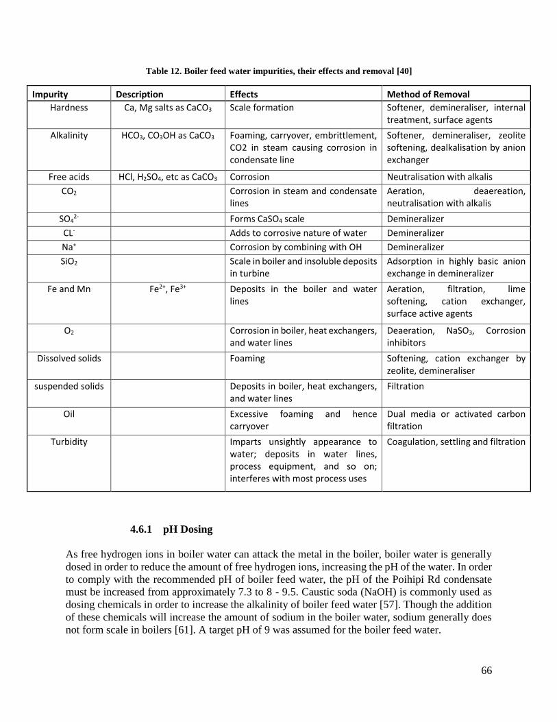
66
Table 12. Boiler feed water impurities, their effects and removal [40]
Impurity Description Effects Method of Removal Hardness Ca, Mg salts as CaCO3 Scale formation Softener, demineraliser, internal
treatment, surface agents
Alkalinity HCO3, CO3OH as CaCO3 Foaming, carryover, embrittlement, CO2 in steam causing corrosion in condensate line
Softener, demineraliser, zeolite softening, dealkalisation by anion exchanger
Free acids HCl, H2SO4, etc as CaCO3 Corrosion Neutralisation with alkalis
CO2
Corrosion in steam and condensate lines
Aeration, deaereation, neutralisation with alkalis
SO42-
Forms CaSO4 scale Demineralizer
CL-
Adds to corrosive nature of water Demineralizer
Na+
Corrosion by combining with OH Demineralizer
SiO2
Scale in boiler and insoluble deposits in turbine
Adsorption in highly basic anion exchange in demineralizer
Fe and Mn Fe2+, Fe3+ Deposits in the boiler and water lines
Aeration, filtration, lime softening, cation exchanger, surface active agents
O2
Corrosion in boiler, heat exchangers, and water lines
Deaeration, NaSO3, Corrosion inhibitors
Dissolved solids
Foaming Softening, cation exchanger by zeolite, demineraliser
suspended solids
Deposits in boiler, heat exchangers, and water lines
Filtration
Oil
Excessive foaming and hence carryover
Dual media or activated carbon filtration
Turbidity
Imparts unsightly appearance to water; deposits in water lines, process equipment, and so on; interferes with most process uses
Coagulation, settling and filtration
4.6.1 pH Dosing
As free hydrogen ions in boiler water can attack the metal in the boiler, boiler water is generally
dosed in order to reduce the amount of free hydrogen ions, increasing the pH of the water. In order
to comply with the recommended pH of boiler feed water, the pH of the Poihipi Rd condensate
must be increased from approximately 7.3 to 8 - 9.5. Caustic soda (NaOH) is commonly used as
dosing chemicals in order to increase the alkalinity of boiler feed water [57]. Though the addition
of these chemicals will increase the amount of sodium in the boiler water, sodium generally does
not form scale in boilers [61]. A target pH of 9 was assumed for the boiler feed water.

67
Equation 39 was used in order to calculate the concentration of caustic soda that should be added
to the boiler feed water in order to achieve the desired pH.
𝑪𝑵𝒂𝑶𝑯 = 𝟏𝟎−(𝟏𝟒−𝒑𝑯𝟐) − 𝟏𝟎−(𝟏𝟒−𝒑𝑯𝟏) (39)
Where:
pH1 = the initial pH of the boiler feed water
pH2 = the desired pH of the boiler feed water
CNaOH = concentration of NaOH that should be added to achieve pH2 (mol/L boiler
feed water)
In order to calculate the amount of caustic soda that should be added to the boiler feed water the
concentration of caustic soda could be converted to a mass flowrate using Equation 40.
�̇�𝑵𝒂𝑶𝑯 = 𝑪𝑵𝒂𝑶𝑯 × 𝑴𝑵𝒂𝑶𝑯 ×�̇�𝑭𝑾
𝝆𝑭𝑾 (40)
Where:
�̇�𝑁𝑎𝑂𝐻 = the mass flowrate of NaOH to be added to the boiler feed water (g/h)
MNaOH = the molar mass of NaOH (39.997 g/mol)
�̇�𝐹𝑊 = the mass flowrate of boiler feed water (kg/h)
ρFW = the density of the boiler feed water (taken as 0.998 kg/L)
4.6.2 Deaeration
As the dissolved oxygen concentration at 0.55 mg/L in the Poihipi Rd condensate is higher than
the recommended boiler feed water limits at 0.07 mg/L, deaeration must be performed on the
condensate. As the solubility of oxygen in water increases with pressure and decreases with
temperature as shown in Figure 39, by increasing the temperature and/or decreasing the pressure,
the oxygen may be desorbed from the water. Deaeration occurs in cylindrical vessels with spray
nozzles inside, the feed water is sprayed into very fine droplets to allow for almost complete
desorption of the oxygen and other gasses. Deaerators when properly operated may reduce the
oxygen concentration of the feed water to below 0.007 ppb [62], orders of magnitude below the
required maximum concentration of 0.007 ppm (mg/L).

68
Figure 39. The solubility of oxygen in water under different temperatures and pressures [40]
It was decided that in order to simplify the deaerator, it should be operated at slightly above
atmospheric pressure, as this will aid in the disposal of oxygen and other gasses from the deaerator.
With reference to Figure 39, it can be seen that for a deaerator operating at 2 psig (14 kPag) will
require the water to be heated to approximately 103°C. As this is very similar to the boiling point
of water at 2 psig, control on the heating will need to be performed in order to ensure minimal loss
of steam with the desorbed gasses. The majority of the heating required to be performed on the
feed water will be done during the preheating of the feed water using SGW as the heat source, as
this is used to heat the water to approximately 100°C. Steam recycled from the boiler will be used
to provide the additional heat required for deaeration, the flowrate of this steam may then be altered
in order to achieve the necessary heating.
The vent rates of steam from the deaerator are typically between 5% - 14% of the steam introduced
to the deaerator [63]. There is a relatively small heating load required to be performed by the steam,
as the feed water is only required to be heated approximately 3°C, corresponding to a relatively
small mass flowrate of steam required. As one purpose of the recycled steam is to carry away the
desorbed gasses, a vent rate of 14% of the recycled steam was chosen to ensure adequate removal
of the gasses.
Provided the deaerator is operated correctly, oxygen scavenger additives such as hydrazine are not
expected to be required.
4.6.3 Blowdown Control of Boiler Water
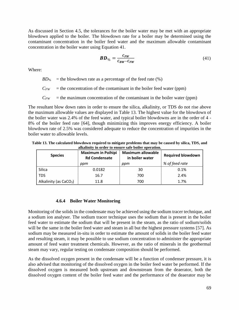
69
As discussed in Section 4.5, the tolerances for the boiler water may be met with an appropriate
blowdown applied to the boiler. The blowdown rate for a boiler may be determined using the
contaminant concentration in the boiler feed water and the maximum allowable contaminant
concentration in the boiler water using Equation 41.
𝑩𝑫% =𝑪𝑭𝑾
𝑪𝑩𝑾−𝑪𝑭𝑾 (41)
Where:
BD% = the blowdown rate as a percentage of the feed rate (%)
CFW = the concentration of the contaminant in the boiler feed water (ppm)
CFW = the maximum concentration of the contaminant in the boiler water (ppm)
The resultant blow down rates in order to ensure the silica, alkalinity, or TDS do not rise above
the maximum allowable values are displayed in Table 13. The highest value for the blowdown of
the boiler water was 2.4% of the feed water, and typical boiler blowdowns are in the order of 4 -
8% of the boiler feed rate [64], though minimizing this improves energy efficiency. A boiler
blowdown rate of 2.5% was considered adequate to reduce the concentration of impurities in the
boiler water to allowable levels.
Table 13. The calculated blowdown required to mitigate problems that may be caused by silica, TDS, and
alkalinity in order to ensure safe boiler operation.
Species Maximum in Poihipi
Rd Condensate Maximum allowable
in boiler water Required blowdown
ppm ppm % of feed rate
Silica 0.0182 30 0.1% TDS 16.7 700 2.4%
Alkalinity (as CaCO3) 11.8 700 1.7%
4.6.4 Boiler Water Monitoring
Monitoring of the solids in the condensate may be achieved using the sodium tracer technique, and
a sodium ion analyser. The sodium tracer technique uses the sodium that is present in the boiler
feed water to estimate the sodium that will be present in the steam, as the ratio of sodium/solids
will be the same in the boiler feed water and steam in all but the highest pressure systems [57]. As
sodium may be measured in-situ in order to estimate the amount of solids in the boiler feed water
and resulting steam, it may be possible to use sodium concentration to administer the appropriate
amount of feed water treatment chemicals. However, as the ratio of minerals in the geothermal
steam may vary, regular testing on condensate composition should be performed.
As the dissolved oxygen present in the condensate will be a function of condenser pressure, it is
also advised that monitoring of the dissolved oxygen in the boiler feed water be performed. If the
dissolved oxygen is measured both upstream and downstream from the deaerator, both the
dissolved oxygen content of the boiler feed water and the performance of the deaerator may be

70
evaluated. If dissolved oxygen concentrations in the boiler feed become too high, it may require
the addition of an oxygen scavenger, such as hydrazine in order to reduce the concentration to
allowable levels.
4.6.5 Reliability of Results
As the wells used at Poihipi Rd are relatively constant with the operation of the Power Plant, the
geometry and length of the steam lines also remained relatively constant. In order to better
understand how the purity of the Poihipi Rd condensate will change with time, results from tests
performed when different wells were used to supply Poihipi Rd with steam. Results from tests
performed on the Poihipi Rd condensate and Poihipi Rd condenser performed from 2007 to 2008
were used to compare with the tests performed for this study. However, as these tests were not
performed with focus on utilizing the condensate as boiler feed water, not all of the species of
interest were tested for. The tests of the three tests performed from 2007 to 2008, and the test
performed for this this study are displayed in Table 14. For brevity, not all of the species tested for
are displayed in Table 14, the full testing results may be found in the appendices.
Table 14. Testing results for the species of interest in Poihipi Rd condensate to assess the variability of the
condensate
Species Units Poihipi Rd
Condensate Poihipi Rd
Condensate Poihipi Rd
Condenser water Poihipi Rd
Condensate
17-Jul-07 30-Apr-08 14-May-08 14-Jun-16 Calcium ppm <0.05 <0.053 <0.053 <0.053
Magnesium ppm <0.01 <0.021 <0.021 <0.021 Total Hardness
(as CaCO3) ppm <0.166 <0.219 <0.219 <0.219
Silica ppm <0.06 - - <0.011
Conductivity µS/cm 24 - - 22
pH pH units 6.67 - - 7.3
Alkalinity (as CaCO3) ppm - - - 11
Iron ppm - 0.032 <0.021 <0.021
Copper ppm 0.002 0.00059 0.00057 <0.000053
It can be seen that the iron and copper concentrations are consistently below the recommended
tolerances displayed in Table 6. The hardness of the water was also seen to be relatively constant
across the tests performed, and would likely meet the boiler feed water tolerances if the blowdown
is designed correctly. The conductivity was only measured in one other test, but was seen to be
relatively concordant with the measurement performed for this study. The pH was also only tested
for in one other test, and the lower pH of 6.67 would require a larger dosage of NaOH in order to
adequately increase the pH. However, as a whole, there was little in the historical testing results
that indicates large variability in the purity of the Poihipi Rd condensate. It is therefore considered
likely that the feed water cleaning system of deaeration, pH dosing, and boiler blowdown will be
sufficient to ensure that the Poihipi Rd condensate is suitable to be used as boiler feed water for a
4.5 bara boiler.

71
4.7 Poihipi Rd Condensate Availability
As the condensate from Poihipi Rd already has several uses on the plant, there are limits on the
amount of condensate which may potentially be used as boiler feed water. Currently the majority
of the condensate created in the shell and tube condensers at Poihipi Rd is used in the cooling
tower at Poihipi Rd. However there is approximately 97 t/h that is available for other plant uses.
Of this, condensate is used to dilute acid for acid dosing on SGW reinjection, used for wash water
in the Te Mihi cooling towers, and sporadically used to refill the cooling towers following an
outage when they have been emptied. The acid dosing requires approximately 18 t/h of the Poihipi
Rd condensate, though an allowance of 25 t/h has been made to allow for water leakage without
system failure, and any other minor uses. The Te Mihi wash water system uses approximately 18
t/h of the Poihipi Rd condensate, though this is highly variable, and is based off the capacity of 4%
of the full steam flow to Te Mihi, as displayed in Figure 40. When refilling of the cooling towers
is required to be performed, the vast majority of the Poihipi Rd condensate is used, as this allows
the cooling tower to be filled relatively fast, minimizing time delays. The use of the Poihipi Rd
condensate to refill the cooling towers is also important, as the clean condensate controls the
bacterial growth within the towers.
Figure 40. The daily average of Poihipi Rd condensate flow to Te Mihi
Due to this, there is an average of approximately 54 t/h of the clean Poihipi Rd condensate available
to be used as boiler feed water during normal operation of the plant. However this flow will likely
stop completely whenever refilling of the cooling towers is required to be performed.

72
5.0 Plant Design and Cost Estimation
In order to quantify any potential benefits from implementing the hybrid gasification/geothermal
plants proposed in Section 2.0, the costs associated with the additional process equipment must be
quantified. New Zealand prices were inflated using the Reserve Bank of New Zealand’s inflation
calculator [65], which uses data from Statistics New Zealand. United States prices were inflated
with reference to the US Government’s consumer price index data. When converting between
2016USD and 2016NZD a conversion factor of 1.42 was used.
5.1 Economic Environment
The availability and costs for landing residues, and the expected sale price of power were
investigated.
5.1.1 Forest Residue Availability and cost
The delivered cost of landing residues increases with increasing delivery distance, the larger the
collection area for the landing residues the higher the average cost for the landing residues will be.
Thus, the larger the size of the gasifier, the higher the relative costs for the landing residues
become, due to the increased feed rate of woody biomass to the gasifier. The delivered costs of
landing residues in New Zealand are based on those reported by Hall and Gifford in a report for
Scion, as displayed in Figure 41 [66]. The delivered costs are given in 2007 NZD/GJ, and it is
assumed in the report that the landing residues have an energy density of 8 GJ/m3. As the calorific
value of radiata pine is assumed to be that of softwoods reported in the New Zealand Energy
Information Handbook [55] at 19.2 GJ/t, the assumed bulk density was calculated to be 416 kg/m3.
Figure 41. The delivered costs for landing residues for different delivery distances, assuming 8 GJ/m3 [66]

73
In order to estimate the current costs of the landing residues correction factors were created based
on the costs of pulp logs. As there is no data available for the changing costs of landing residues,
it was assumed that the costs of landing residues would fluctuate with the costs of pulp logs, as
displayed in Figure 42. This method is imperfect, as pulp logs are not a direct substitute for landing
residues. Landing residues are predominantly used as a bioenergy fuel, whereas pulp log are used
to make paper. However, in the absence of information on price fluctuations for landing residues,
it is believed that the price for pulp logs and landing residues will be correlated, as they are both
low quality wood. The yearly average for the high and low prices of pulp logs are displayed in
Figure 42, using data from the Ministry of Primary Industries [67]. From this, the low and high
cost estimates for the delivered costs of landing residues purchased in 2016 would be increased by
21% and 13% respectively from the price estimates for 2007. As the inflation from 2007 is
approximately 19%, the correction factors of 1.21 and 1.13 were deemed sensible.
Figure 42. Yearly average prices for radiata pine pulp logs in New Zealand [68]
The Central North Island is home to the largest forestry sector in New Zealand with approximately
34% of the planted forest estate [69]. As can be seen in Figure 43, there are extensive planted
forests located relatively close to the Wairakei geothermal field as of 2008, and the Central North
Island still has the largest amount of forestry in New Zealand [66] In order to estimate the delivered
cost of the landing residues the following assumptions were made:
The density of forest plantations is constant within the area of residue collection
The density of the forest plantations used is that of the Taupo Central District
The collection area is circular around Wairakei
That forestry residue distribution (t/ha) is constant for all forestry plantations
That the difference in forestry plantation area in 2014 and 2016 is negligible for the chosen
area of forestry

74
Figure 43. The distribution of planted forests in the North Island as of 2008, modified from [69].

75
The amount of landing residues available in New Zealand for 2016-2020 has been estimated at
1,223,671 t/year [66]. The total forestry plantation area in New Zealand has been estimated to be
1,746,573 ha in 2014 [69]. From this, it was calculated that each hectare of forest plantation
produces an average of 0.7 t/year of landing residues, based on the assumption of negligible change
in plantation area between 2014 and 2016.
The Taupo District has a total area of 697,000 ha which encompasses an estimated 172,554 ha of
plantation forest area in 2014[69]. From this, it can be calculated that each hectare of land in the
Taupo District produces an average of approximately 0.173 t/year of landing residues. The area
for landing residue collection could then be estimated using Equation 42.
𝑨 =�̇�
𝑾𝒓 (42)
Where:
A = the area required for landing residue collection for use at Wairakei (km2)
�̇� = the required mass input of landing residues (t/year)
Wr = the landing residue production rate (17.3 t/year/km2 for Taupo Central District)
From the required landing residue collection area calculated using Equation 42, the average
distance for the landing residues to be transported could be estimated. As it is assumed that there
is constant landing residue distribution within the area of residue collection, and that this collection
area was circular; the average transportation distance would be given by the radius of a circle with
half the area required for residue collection, as displayed in Equation 43.
𝑫 = 𝒇𝒘√𝑨
𝟐𝝅 (43)
Where:
D = the average transportation distance for landing residues (km)
fw = the wiggle factor
It is noted that the distance calculated is the Euclidean distance to the Wairakei site, and not the
actual travel distance. In order to account for this a correction factor is used to convert between
straight line distances and actual transport distances, called a “wiggle factor”. Commonly a wiggle
factor of 1.2 is used [70], however it is believed that this will underestimate the travel distance,
due to the lack of relatively straight roads surrounding Taupo. By comparing the expected travel
distances with the Euclidean distances surrounding the Wairakei site, a wiggle factor of 1.35 was
deemed appropriate to correct the expected travel distances. However, it is also noted that there is
a high density of planted forests in close proximity to the Wairakei site, and therefore distances
estimated may be larger than required due to the assumption of constant forest distribution in the
Taupo District. A detailed investigation involving transport routes from forest plantations close to
Wairakei that could meet the landing residue requirements would need to be performed in order to
more accurately estimate landing residue transport distances.

76
From the average transportation distance calculated using Equation 43, the average transported
cost of the landing residues could be calculated using Figure 41 and inflated based on the inflation
of pulp logs. The Equations for the high and low estimates for the delivered costs have been
modified for the increasing cost of landing residues based on the cost of pulp logs and are displayed
in Equation 44 and Equation 45 respectively.
𝑪𝑳𝑹,𝑯𝒊𝒈𝒉 = 𝟎. 𝟎𝟐𝟒𝟒𝑫 + 𝟒. 𝟐𝟒 (44)
𝑪𝑳𝑹,𝑳𝒐𝒘 = 𝟎. 𝟎𝟏𝟕𝟕𝑫 + 𝟑. 𝟐 (45)
Where:
CLR,High = high estimate for the delivered landing residues (2016 NZD/GJ)
CLR,Low = low estimate for the delivered landing residues (2016 NZD/GJ)
When forecasting prices for the cost of landing residues, the inflation rates calculated using the
radiate pine pulp logs were again used. The high and low prices for the landing residues were
determined using this forecasting, and the average of these two prices was used as the estimated
price for the landing residues for the economic evaluations of the hybrid configurations.
5.1.2 Sale Price of Power
In order to evaluate the financial benefits from implementing any of the hybrid configurations, the
price that the additional power may be sold at was estimated. Price forecasting already performed
by Contact Energy staff was used in order to estimate the yearly average wholesale price of power.
However, as this price forecasting only extended to 2036, the price of power for years beyond this
had to be extrapolated from the price estimates provided by Contact Energy, as displayed in Figure
44. Clearly the price estimates for the years beyond 2036 have a greater uncertainty associated
with them than those for 2016-2036.

77
Figure 44. The wholesale prices of power used for the economic evaluations of the hybrid configurations
5.2 Additional Process Equipment and Modifications Required
As the different hybrid configurations require different process equipment and different
modifications to be performed to the existing equipment at the Wairakei Geothermal Field, there
will be different capital costs associated with each of the hybrid configurations. However, the
gasifier and associated equipment is common to all of the configurations.
5.2.1 Gasification and Landing Residue Pre-treatment
The following equipment is required for every hybrid configuration:
Wood chipper or hog
The landing residues need to be chipped into a form suitable for feeding into the gasifier.
Wood chip dryer
Drying of the wood chips will be performed in order to reduce the moisture content of the
wood to a level appropriate for the gasifier.
Wood Chip Conveyors
Wood chip conveyors will be required in order to transport the wood chips to the dryer and the
gasifier.
Wood Chip Storage

78
Wood chip storage will likely be required in order to buffer the syngas production to the
periodical landing residue deliveries.
Gasifier
A gasifier is used in order to convert the chipped and dried landing residues into syngas.
5.2.2 Superheating Geothermal Steam
In order to superheat the IP geothermal steam for use in modified MP turbines, it is expected that
the following process equipment and modifications will be required:
Furnace
The furnace will be used to transfer the heat from syngas combustion to the geothermal IP
steam in order to increase its temperature to 350°C. The furnace will also require a fan in order
to provide the air required for syngas combustion.
Modification of MP turbines and associated equipment
As the MP turbines and associated equipment are not designed to operate using superheated
steam, modifications will be required in order to utilize superheated steam in these turbines.
Returning turbines to service
As operating the MP turbines on superheated steam instead of IP steam will reduce the mass
flowrate of steam to these turbines, there will be additional unused IP steam to utilize at the
Wairakei A and B Stations. This additional steam will require some turbines at Wairakei which
have been removed from service to be refurbished and recertified.
5.2.3 Boiling Poihipi Rd Condensate
In order to generate additional IP steam by boiling Poihipi Rd condensate, the following process
equipment and plant modifications will be required:
Water treatment
As described in Section 4.6, it is expected that derearation and pH dosing will need to be
performed in order to ensure that the Poihipi Rd condensate will meet the water purity
requirements to be used as boiler feed water.
Condensate preheater
A heat exchanger will be required in order to preheat the Poihipi Rd condensate using SGW,
in order to increase efficiency and facilitate deaeration.
Pumping
Pumping of the geothermal condensate will need to be performed in order to achieve the
pressure required for both deaeration and the boiler.
Boiler

79
A boiler will be required in order to vaporize the Poihipi Rd condensate. Fans will also be
required in order to supply the required air for syngas combustion.
Returning turbines to service
In order to utilize the additional steam generated in the boiler, it is expected that turbines that
have been removed from service at Wairakei will need to be refurbished and recertified.
5.2.4 Boiling IP SGW
In order to use IP SGW at its boiling point as a feed for a boiler, the following process equipment
and modifications are expected to be required:
Boiler
A boiler will be required in order to vaporize some of the IP SGW to produce additional IP
steam.
Returning turbines to service
Turbines which are currently removed from service will need to be refurbished and recertified
in order to utilize the additional steam being produced in the boiler.
5.2.5 Heating Additional SGW to use in the Binary Plant
It was decided that the only process equipment required for this configuration was the furnace used
to heat the T-line SGW, and the fan to provide air to the furnace. As two sources of SGW intersect,
it was assumed that very little piping would be required, as the heated T-line SGW could
potentially be added to the X-line SGW where the two lines intersect.
5.3 Equipment Design and Capital Cost Estimation
Much of the cost estimation performed in this section was performed using the First
Approximation Costing Technique or FACT method [71]. This method can be used to estimate
the cost of many types of process equipment from the required equipment capacity, based on cost
information from vendors.
5.3.1 Landing Residue Pre-treatment and Handling
All of the different hybrid configurations described in Section 2.0 utilize a dual fluidized bed
gasifier to provide syngas. Because of this, the same method for sizing costing this gasifier and
feed handling equipment common to all the configurations were used for each configuration,
though the actual size of the gasifier and associated equipment will vary. The gasifier and the
associated feed equipment were scaled based on the amount of wet wood feed used.

80
5.3.1.1 Size Reduction of Landing Residues
As the biomass input to the DFB gasifier must be reduced in size to smaller than 35 mm in diameter
to be used in the DFB gasifier, size reduction technologies are required [72]. Commonly three
types of size reduction machinery are used to produce the wood chips required for gasification:
disc chippers, drum chippers, and hammer mill hogs.
Disc chippers reduce the size of the biomass by using straight knives attached to a heavy spinning
disk, as displayed in Figure 45. Disc chippers are the most commonly used chippers in the pulp
industry, but the size of the wood chips generated is more variable than with other size reduction
methods.
Figure 45. Diagram of a disc chipper [73]
Drum chippers utilize a rotating cylinder with radially mounted knives in order to chip wood, a
diagram of a drum chipper is displayed in Figure 46. Drum chippers are able to process a wide
range of feed materials, and the size of the wood chips produced may be controlled using a screen
to stop oversized chips [74].

81
Figure 46. A diagram of a drum chipper [73]
Hammer mill hogs reduce the size of biomass by hammering the biomass feed with blunt tools, a
diagram of which is displayed in Figure 47. Sand and stones are inevitably present with the
biomass feed which can serve to blunt the knives employed in chippers, hogs avoid this problem
by using blunt tools such as hammers. Like drum chippers, hammer mill hogs may control the size
of the wood grind can be controlled with a built in screen [74].
Figure 47. A diagram of a hammer mill hog [73]
Costing of the chipper

82
The maximum diameter of the landing residues was assumed to be 0.5m, and the maximum length
of the landing residues was assumed to be 3m in order attain a cost estimate for the chipper. These
size estimates were based a size distributions of logging residues in Appalachia, West Virginia
[75].
After consulting with a New Zealand wood chipper manufacturer, a 75” bottom discharge 4 knife
disc chipper was recommended, based on the estimated size of the landing residues[76]. This
chipper can process logs with a maximum diameter of 560mm, and produces chips at 19 mm. The
life of the chipper was given at approximately 84000 hours, with a maximum flowrate of 50 t/h of
wet wood. The budget price for one chipper delivered to the Wairakei site was quoted as $278,070
GSTinc, which includes:
Two 150 kW electric motors
Motor drive base
Two sets of vee belts
Vee belt pulleys, one driven from each motor, and one for the chipper shaft
One knife system
One babbitting jig
As a large chipper is required in order to handle the diameter of the landing residues, the cost of
the chipper is discretized based on the maximum capacity of the chipper. Therefore the costing for
the chipper was performed by calculating the amount of identical chippers required based on the
mass flowrate of landing residues, and the maximum capacity of the chipper.
As the chippers have an estimated useful life of 84000 hours, it may be required to purchase
additional chippers throughout the life of the hybrid plants. The price of additional chippers were
calculated to inflate at 3% annually in order to estimate the cost of the additional chippers
throughout the life of the hybrid plants.
5.3.1.2 Drying
The typical moisture content of woody biomass is between 50% - 60% wet basis (WB) [77], and
as biomass gasification requires a moisture content of between 10% - 20% WB [78], drying is
required to be performed on the biomass prior to gasification. A moisture content of 15% (WB)
was chosen for the biomass feed for the gasifier. As described in Puladian’s thesis [43], after
comparing three common types of industrial dryers: rotary, pneumatic, and packed moving bed; a
co-current rotary cascade dryer was selected, diagrams of which is displayed in Figure 48 and
Figure 49. Rotary cascade drum dryers utilize longitudinal flights installed on the inner surface of
the dryer to ensure even drying of the wood chips. The rotary drum dryer was selected to perform
the biomass drying due to the large capacity of rotary dryers, the fact that rotary dries are relatively
insensitive to biomass size, and hot flue gas available from the combustion of char and syngas that
can be used as the drying medium. It was decided by Puladian, that the rotary dryer should employ
a co-current flow of biomass and flue gas drying medium, as a counter current arrangement may
heat the biomass to the auto-ignition temperature of wood (260 - 280°C).

83
Figure 48. Diagram of a cascade co-current rotary drum dryer [79]
Figure 49. A cross section of a cascade rotary drum dryer [79]
In order to size the rotary drum dryer, the temperature of the wet biomass, and the ambient air
were both assumed to be 10°C.
Costing the rotary drum dryer
The method for estimating the capital cost of a rotary drum dryer was based on that used by
Penniall in his Master’s Thesis investigating the potential for a gasification plant in the wood
process industry [80]. This method was developed due to the extremely high capital costs that were
estimated using other methods for rotary drum dryers when the moisture content of the inlet wood
is high [81]. Penniall’s cost estimate was developed using estimates from New Zealand
manufacturers, and has been modified to account for inflation as displayed in Equation 46.
𝑪𝑫𝒓𝒚𝒆𝒓 = 𝟒. 𝟐 × 𝟏𝟎𝟓�̇�𝒎𝒐𝒊𝒔𝒕𝒖𝒓𝒆 + 𝟒. 𝟐 × 𝟏𝟎𝟓 (46)
Where:

84
CDryer = the installed capital cost of the dryer (2016 NZD)
�̇�𝑚𝑜𝑖𝑠𝑡𝑢𝑟𝑒 = the mass flowrate of moisture removed from the wood (t/h)
5.3.1.3 Biomass Storage and Handling Equipment
The feed handling required for a biomass gasification plant is often ignored in the design of woody
biomass gasification plants, with the exception of the chipping and drying of the biomass. The
biomass storage and metering for this design is loosely based on that designed by Worley and Yale
in a gasifier technology assessment commissioned by the National Renewable Energy Laboratory
(NREL) [82].
The designed biomass storage and metering system consists of a belt conveyor, a storage bunker,
two transfer screw conveyors, and a storage hopper. It is believed that the landing residues should
be chipped immediately upon delivery, as wood chips may be more easily stored and moved within
the plant than the landing residues. The belt conveyor will feed the landing residues into the
biomass chipper. The chipped biomass will then be deposited in a storage bunker, as storage of the
biomass will be simpler when it is wet, as dry wood chips are susceptible to moisture
contamination. The first transfer screw conveyor be used to transport the wet wood chips to the
rotary dryer. The wood chip dryer will discharge into the second hopper, and the electro vibrating
feeder will be used to meter the dried wood chips to the gasifier. The second transfer screw
conveyor will be used to transport the dried biomass into the gasifier. The biomass storage and
preparation system is displayed in Figure 50.
Belt Conveyor
Drum Chipper
Bunker
Transfer Screw Conveyor Rotary Drum Dryer
HopperTransfer Screw Conveyor
Wood delivery
Figure 50. The biomass feed preparation and storage equipment
Costing of hoppers and feeders
The storage bunker for the wet wood chips was designed to store sufficient wood chips for two
days of continuous gasifier operation, in order to avoid losses that would be incurred due to
irregular wood supply. The dry wood chip storage for the gasifier feed in the hopper was sized to
have volume enough for ½ an hour of wood chip feed to the gasifier. The bulk density of the wet
wood chips was assumed to be 300 kg/m3 [83].
The cost of bunker storage has been investigated for grain storage on cattle farms [84], and was
altered for wood chip storage. The cost for grain bunkers was given as $59.72 2006USD/short ton

85
of grain, the density of wheat grain was taken as 770 kg/m3 [85]. This yielded a value of $168.96
2006USD/t wood chips which converts to 260.83 2016NZD/ton wet wood chips.
The cost of the storage hopper was estimated by assuming the cost would be similar to that for
atmospheric storage vessels. The FACT method was then employed in order to estimate this cost
[71]. The cost for atmospheric storage vessels may be estimated as 1.25 2010USD/gallon. Using
a correction value of 1.102 for inflation, and the currency conversion factor, the cost of the storage
hopper may be estimated as 515.8 2016NZD/m3.
Costing of conveyors
The drum chipper has an entry width of 1400 mm based on the design specifications given by a
supplier, the belt conveyer will be designed to have a similar width. By using the First
Approximation Costing Technique (FACT) Method, costs for belt conveyors may be estimated, as
displayed in Figure 51. A conveying distance of 10 m was assumed to be sufficient to feed into
the chipper.
Figure 51. The estimated cost (December 2004 NZD) for belt and bucket conveyors based on the FACT
Method
The diameter for the transfer screw conveyer was based on manufacturers data found for the
expected wood chip transfer capacity for different screw diameters, as displayed Table 15 [86]. A
conveyer length of 15 m was estimated for both of the transfer screw conveyors.

86
Table 15. Manufacturer’s data for wood chip transfer screw conveyers [86]
Model WLS150 WLS200 WLS250 WLS300 WLS400 WLS500
Screw Diameter mm 150 184 237 284 365 470 Casting pipe diameter mm 180 219 273 351 402 500
Operating angle ° <30 <30 <30 <30 <30 <30 Maximum delivery length m 12 13 16 18 22 25
Capacity t/h 3 7 9 13 18 28 Motor (Length > 7m) kW 1.5 2.2 3 5.5 11 11 Motor (Length < 7m) kW 2.2 3 4 7.5 15 15
The FACT method could be used to estimate the cost of the wood chip screw conveyor, also known
as a transfer auger, in a similar method to that for the belt conveyor. The estimated costs for auger
conveyers are displayed in Figure 52.
Figure 52. The estimated cost (December 2004 NZD) for auger and apron conveyors based on the FACT
Method
As the costs for the belt conveyor and the wood chip transfer augers do not include the cost for the
motors required, this was calculated separately. Costs for motors can be calculated based on the
power requirement of the motor using the FACT Method. Power requirements for the wood chip
auger can be estimated from Table 15, provided the required wood chip flowrate, and the length
of the auger are known. By researching the expected power requirements for a variety of belt
conveyor sizes, it was assumed that the belt conveyor feeding the chipper with a width of 1400
mm would likely have a power requirement of approximately 11 kW [87]. Once the power
requirement of the conveyor motors are estimated, the cost for these motors can be calculated using
the FACT method shown in Figure 53.

87
Figure 53. The estimated cost (December 2004 NZD) for electric motors based on the FACT Method
5.3.2 Gasification
A dual fluidized bed gasifier was chosen to perform the gasification step as the Chemical and
Process Engineering Department at the University of Canterbury has extensive knowledge of this
type of gasifier. The gasifier consists of two fluidized beds, two cyclones, two burners, a chute and
a siphon to circulate the bed material.
Costing of the dual fluidized bed gasifier
A method used at the University of Canterbury to estimate the capital costs associated with a dual
fluidized bed gasifier was initially developed by Rutherford for his Masters’ Thesis investigating
the heat and power applications of biomass gasifiers in New Zealand’s wood industry [88]. Due
to a lack of information for the cost histories for gasifiers, Rutherford developed a “ground up”
approach to estimate the cost based on the individual components of the gasifier and installation
factors. As the scaling factors that may be applied to gasification reactors are seen to vary widely,
leading to uncertainty in any capital costs generated, this “ground up” method will be used here.
As described by Rutherford in his Master’s Thesis, the gasifier is broken down into its component
pieces, and the superficial velocity of the gas in each of these components used as in the lab scale
DFB reactor at the University of Canterbury displayed in Table 16. The components that make up
the gasifier are: the bubbling fluidized bed (BFB) reactor, the entrained flow fluidized bed (CFB)
reactor, a chute, a siphon, two cyclones, two gas burners, and a blower. The BFB reactor, CFB
reactor, chute, and the siphon are all to be lined with 100mm of hot refractory and a further 150mm
of cold refractory lining. It was assumed that the geometries of all the vessels involved was to be

88
cylindrical, and ratios for the dimensions of the vessels are also taken from Rutherford [88]. The
BFB reactor was designed to have a height 2.4 times its diameter, and the CFB reactor was
designed to be 2m longer than the BFB reactor to allow space for the chute, siphon, and cyclone.
Table 16. The assumed superficial gas velocities for the University of Canterbury’s dual fluidized bed gasifier
Vessel Gas Velocity Entrained flow Fluidized Bed 7 m/s Bubbling Fluidized Bed 1.5 m/s Chute 0.15 m/s Siphon 0.15 m/s
The cost of the blower for the gasifier was found using Equation 47.
𝑪𝒃𝒍𝒐𝒘𝒆𝒓 = 𝟕𝟕𝟏𝑸𝒂𝒊𝒓 + 𝟐𝟒𝟎𝟎 (47)
Where:
Cblower = the cost for the blowers installed in the gasifier (2006 NZD)
Qair = the volumetric flowrate of air through the CFB (m3/s)
The cost of the steel casings for the vessels of the gasifier was found using Equation 48
𝑪𝒄𝒂𝒔𝒊𝒏𝒈 = (𝟑𝟗𝟓𝟐𝑫𝑽 + 𝟗𝟔𝟓)𝑯𝒗(𝟎.𝟗𝟕𝟒𝟗−𝟎.𝟎𝟓𝟏𝟖𝑫𝒓)
(48)
Where:
Ccasing = the cost for the steel casing on the vessels of the gasifier (2006 NZD)
Dv = the diameter of the vessel (m)
Hv = the height of the vessel (m)
The cost for the cyclones used in the gasifier was found using Equation 49
𝑪𝒄𝒚𝒄𝒍𝒐𝒏𝒆 = 𝟐𝟑𝟑𝟎𝑸𝒄𝒚𝒄𝒍𝒐𝒏𝒆𝟎.𝟗𝟏𝟐
(49)
Where:
Ccyclone = the cost for the cyclone in the gasifier (2006 NZD)
Qcyclone = the flowrate of gas through the cyclone (m3/s)

89
The cost for the refractory lining on the vessels in the gasifier is found using Equation 50.
𝑪𝒓𝒆𝒇𝒂𝒄𝒕𝒐𝒓𝒚 =𝟒𝟓
𝟐𝟖𝒎𝒉𝒇 +
𝟐𝟖
𝟏𝟓𝒎𝒄𝒇 (50)
Where:
Crefractory = the capital cost for the refractory lining on the gasifier (2006 NZD)
mhf = the mass of hot refractory lining required (kg)
mcf = the mass of cold refractory lining required (kg)
The density of the hot and cold face refractory linings were taken to be 960 kg/m3 and 480 kg/m3
respectively [89].
The cost for the burners required in the gasifier was based on the cost estimate used by Penniall
for his Master’s Thesis [80] where burners were costed at 12,000 2006 NZD each.
In order to account for the inflation from 2006 an inflation factor of 1.22 were used to convert the
estimates to 2016 NZD.
5.3.3 Returning Steam Turbines to Service
In order to utilize steam that is generated in a boiler, or the steam that is saved by the lower mass
flowrate required for superheated steam in a modified geothermal turbine, steam turbines at the
Wairakei Power Plant will likely need to be brought back into service. Currently there are two
turbines that have been removed from service at Wairakei, G1 and G8. G1 is an IP steam turbine,
which uses 241 t/h of IP steam to produce 11.2 MWe at full load. G8 is an LP steam turbine, which
uses 140 t/h of LP steam to produce 11.2 MWe at full load. As there is not sufficient LP steam to
completely load the LP steam turbines currently in service, the LP turbine, G7, is almost
continuously unloaded. Due to this, it is assumed that LP steam may be used in G7 without
requiring additional LP turbines to be returned to service. Estimates for the cost of recertifying
some of the turbines at Wairakei have been performed by Contact Energy employees, and are
displayed in Table 17.
Table 17. The estimated costs of recertifying turbines at the Wairakei Power Plant
Turbine Type of Turbine
Estimated cost (2016 NZD)
Current Status
G1 IP $760,000 Removed from service 2014 G4 IP $659,000 In service
G7 LP $520,000 In service G10 LP $599,000 In service G11 MP $1,245,000 In service
G13 MP $1,120,000 In service

90
In order to bring G8, back into service the two oil separators that are used on the LP turbines would
need to be replaced, as these have been removed. A rough estimate of $100,000 has been provided
by staff at Wairakei to replace each of these separators. The base cost of refurbishing and
recertifying G8 was based on the cost of recertifying G7, at $520,000 as they are both the same
type of turbine. Therefore, the estimate for the total cost of bringing G8 back into service is
estimated as $720,000.
Currently, the turbines in the Wairakei A Station, need recertification every 5 years, due to this,
any additional turbines brought back into service will incur the cost of this recertification. The
base cost of recertifying G1 and G8 were assumed at $760,000 and $520,000 respectively. These
costs were then inflated using an assumed annual inflation of 3%, for the 5 yearly recertification.
5.3.4 Furnaces and Fans
Furnaces are designed to be used to superheat the geothermal steam, and to heat the SGW in T-
line for use in the Wairakei Binary Plant. The design of the furnaces was based on that given in a
report on Process Equipment Cost Estimation by Loh, Lyons, and White for the National Energy
Technology Laboratory [90]. Price estimation is performed on furnaces of differing duties, where
it is assumed that the design temperature is approximately 400°C and a design pressure is
approximately 35 bara. As the pressure of the geothermal steam and SGW is lower than 35 bara,
at 4.5 bara and 9 bara respectively, the high design pressure may lead to an overdesigned furnace
with an inflated estimate for the capital cost. The tube material is designed to constructed using
A214 carbon steel that is electro-resistance welded.
The furnace will also require fans in order to supply the necessary air to combust the syngas. The
fans were assumed to be centrifugal, and a pressure ratio of 0.95 was designed for the ambient air
and the air supply to the furnace, with a resulted in an assumed pressure increase of 5.3 kPa.
Costing the furnace
The cost estimation of the furnace was performed with reference to the report by Loh, Lyons, and
White, where the cost may be estimated from the heating duty required to be performed by the
furnace. The cost of the furnace in 1st Quarter 1998 USD can be found using Figure 54.

91
Figure 54. The estimated cost (1st Quarter 1998 USD) for furnaces based on the heat duty of the furnace [90]
The estimated purchase cost for the furnace found in Figure 54 was then inflated and converted
into 2016 NZD.
Costing of the Furnace Fans
The cost estimation was performed under the assumption that centrifugal fans would be used in
supply the required air flow to the furnace. The method of costing the furnace fans was performed
using the FACT method, where the pressure increase and volumetric flowrate of air are used to
estimate the capital cost of the fans [71]. The cost of the fans could then be estimated using
Equation 51.
𝑪𝒇𝒂𝒏 = 𝑭𝑷(𝟗𝟕𝟗�̇�𝒂𝒊𝒓 + 𝟑𝟎𝟒𝟖) (51)
Where:
FP = the centrifugal fan cost correction factor
Cfan = the cost of the fan (2016NZD)
�̇�𝑎𝑖𝑟 = the volumetric flowrate of the air (m3/s)
The cost correction factors for the pressure increase delivered by the fans is displayed in Table 18.

92
Table 18. The cost correction factors for centrifugal fans [71].
Pressure increase (kPa) Centrifugal fan cost correction factor (Fp)
1 1 2 1.15 4 1.3 8 1.45
16 1.6
By interpolating the values for the correction factors, it was found that a correction factor of 1.36
should be applied for a pressure increase of 5.3kPa.
5.3.5 Modifying Existing MP Steam Turbines to use Superheated Steam
In order for superheated steam to be utilized in the MP steam turbines currently at Wairakei,
significant modifications would need to be performed to the turbines to allow for the increased
temperature and velocity of the steam. The modifications that are expected to be required are as
follows:
Changing the turbine blades
The velocity of the steam passing through the MP turbine will be increased, due to the fact that
there is a reduction of the amount of steam condensation occurring in the turbine. Due to this,
the blade incidence angles will no longer be optimized for the higher steam velocity. Therefore
it is expected that new turbine blades will have to be purchased for the modified turbines.
New diaphragms and nozzles
Similar to the requirement for new turbine blades, new diaphragms and nozzles are expected
to be required for the steam turbines, in order to optimize the design of the nozzles.
Steam turbine casings
The design of the maximum temperature of the superheated steam was made with reference to
the suggestions made by Morris in his investigation into superheating geothermal steam for
use in existing steam turbines [38]. However, this temperature was chosen based on the creep
range of low alloy steel, and many the casings of the steam turbines are grade 10 grey cast iron,
these casing will prove to be incompatible with the higher temperature steam. At temperatures
approaching 350°C, grey iron is expected to be an unsuitable material for the steam turbine
casings [91]. Due to this, new casing will need to be created, requiring moulds to be created to
cast the casings.
Valves
The valves used at Wairakei have valves and seals constructed from PTFE. The operating limit
of this material is approximately 200°C, with an absolute limit of 250°C [38]. Due to this new
valves and hydraulics would be required in order to utilize superheated steam at 350°C.
Insulation and oil cooling

93
Due to the higher temperatures of the steam entering the MP turbine, added insulation will be
required to avoid exposure dangerously high temperature equipment and pipelines. It is
believed that the fiberglass and calcium silicate currently used as insulation at Wairakei will
remain suitable for use as insulation at the elevated temperatures, though the thickness of the
insulation will have to be increased. The cooling oil flow across the hot end of the turbine is
also expected to increase in order to dissipate the higher heat flow.
Installation
It was assumed that once the parts required to perform the modifications to the MP turbines
had been fabricated and delivered, there would be a three week installation period. There would
therefore be an associated loss of revenue from removing the MP turbines from service to
perform these modifications.
Costing MP turbine modifications
As there is very little information on the costs associated with modifying geothermal steam
turbines to operate using superheated steam, the costs for these modifications are rough estimates
with a large associated uncertainty.
Turbine blades
It was assumed that the new turbine blades could be costed based on the cost of the current set of
turbine blades, as the materials and method of construction would likely be the same. The current
MP turbines have 15 rows of blades, 8 in the IP section of the turbine and 7 in the LP section. The
first 10 rows have 250 blades each, and the remaining rows have 140 blades each. The blades on
the IP rows are estimated at $1000 each, and the blades on the LP rows are estimated at $5000
each. The cost of the new blades are therefore estimated at 8,000,000 2016NZD for each turbine.
Diaphragms and nozzles
The cost of the diaphragms nozzles are estimated at $1,000,000 for a set, which includes the cost
of the nozzles. The diaphragms will likely be fabricated from welded steel components, which
would prove to be costly.
Steam turbine casings
The steam turbine casings are estimated at $4,000,000 each, these are expected to be very
expensive, due to the necessity to create moulds in order to cast the casings.
Valves, insulation, and oil cooling
It was assumed that the costs associated with the valves, insulation and oil cooling would be
included in the costs associated with the minor material of the furnace.
Installation
It was assumed that staff at Wairakei would be able to perform the modifications to the turbine(s),
and therefore there would be no labour cost associated with the installation. However, as it was
assumed that there would be a three week installation period for the turbines, there is a maximum
loss of 15120 MWh for each turbine removed from service.

94
5.3.6 Boiling Poihipi Rd Condensate
In order to generate additional IP steam using the Poihipi Rd condensate as a boiler feed water, it
is expected that two pumps, a preheater, a boiler, a deaerator, and chemical injection apparatus
will be required. There are also limits on the amount of the Poihipi Rd condensate that may be
used, which must be taken into account when designing the size of the process equipment.
5.3.6.1 Condensate Pumps
As the condensate from the Poihipi Rd Power Plant is available at approximately 7.8 kPa, pumping
will need to be performed in order for this condensate to be used as boiler feed water. In order to
facilitate deaeration, the condensate must first be increased in pressure to 1.15 bara for oxygen
desorption. The condensate will then be increased in pressure to 4.5 bara for the boiler feed water.
Two stages of pumping are therefore required to be performed on the Poihipi Rd condensate in
order for it to be used as boiler feed water
Costing the condensate pumps
The costs for the condensate pumps were estimated using the FACT method [71], using the cost
estimates displayed in Table 19. The costs for the pumps displayed in Table 19 are for heavy duty
hydrocarbon pumps, as carbon steel pumps will likely be used, price of the pump will be
approximately 70% of that for the hydrocarbon pumps.
Table 19. The cost of pumps and motors for single stage pumps [71].
Pump power Cost
HP 2006USD
0 - 10 10000
10 - 50 h 10000+150/HP
50 - 500 15000 + 175/HP
500 - 1000 25000 + 200/HP
> 1000 40000 + 225/HP
The power requirement of the pumps was taken from the UniSim model for the boiling of the
Poihipi Rd condensate, which assumes a 75% adiabatic efficiency for the condensate pumps.
5.3.6.2 Condensate Preheating
In order to maximize the amount of steam that may be generated in the boiler, preheating on the
steam turbine condensate is designed to be performed using heat from high temperature SGW. The
Karapiti SGW reinjection system was used as the basis for SGW resources available for preheating
the condensate, due to the proximity of this reinjection system to the source of condensate at

95
Poihipi Rd. This SGW is available at approximately 105°C, and as there is an average flow of
approximately 3000 t/h, this will be sufficient to adequately preheat the condensate as there is only
54 t/h of condensate available for use from Poihipi Rd. As the preheater will be similar in essence
to the preheaters and vaporizers used in the Wairakei Binary Plant which uses SGW to heat pentane
for an organic Rankine cycle, the design of the condensate preheater is based on the binary plant
heat exchangers. A shell and tube heat exchanger with carbon steel tubes will be used to preheat
the condensate. A shell and tube heat exchanger will be used to increase the temperature of the
condensate from approximately 40°C to 100°C. The flowrate of SGW to the preheater was
designed to ensure the exit temperature of SGW from the preheater was greater than 90°C, based
on the design of the Wairakei Binary Plant heat exchangers.
Costing the tubular preheater
The FACT method was used in order to estimate the cost for the preheater heat exchanger [71].
The operating pressure of the heat exchanger, the heat duty of the heat exchanger, and the type of
heat exchange occurring were used to estimate the heat exchange area.
The heat flux typical of different types of heat exchange is displayed in Table 20.
Table 20. Heat flux typical for different types of heat exchange in tubular heat exchangers [71]
Type of heat exchange Flux (Btu/h/ft2)
Gas to Gas 3000
Liquid to Liquid 8000
Phase Change 10000
Steam Condensing 12000
By then using the heat duty of the preheater, which is calculated by the UniSim model, the heat
exchange area could be calculated.
The cost of the heat exchanger in 2006 USD could then be estimated using the different prices
displayed in Table 21. The Karapiti reinjection pumps, which would likely provide the SGW used
to preheat the Poihipi Rd Condensate, had an average outlet pressure of approximately 19.7 bara
(285 psi) and a maximum outlet pressure of 27.2 bara (394 psi) the operating pressure of 300-600
psi was used for the preheater.
Table 21. The prices for heat exchangers based on their design pressures [71].
Design pressure Cost of heat exchanger
Psi 2006 USD
0-300 10000+35/ft2
300-600 10000+40/ft2
>600 10000+45/ft2
5.3.6.3 Boiler and Feed Water Cleaning
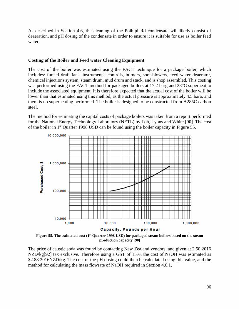
96
As described in Section 4.6, the cleaning of the Poihipi Rd condensate will likely consist of
deaeration, and pH dosing of the condensate in order to ensure it is suitable for use as boiler feed
water.
Costing of the Boiler and Feed water Cleaning Equipment
The cost of the boiler was estimated using the FACT technique for a package boiler, which
includes: forced draft fans, instruments, controls, burners, soot-blowers, feed water deaerator,
chemical injections system, steam drum, mud drum and stack, and is shop assembled. This costing
was performed using the FACT method for packaged boilers at 17.2 barg and 38°C superheat to
include the associated equipment. It is therefore expected that the actual cost of the boiler will be
lower than that estimated using this method, as the actual pressure is approximately 4.5 bara, and
there is no superheating performed. The boiler is designed to be constructed from A285C carbon
steel.
The method for estimating the capital costs of package boilers was taken from a report performed
for the National Energy Technology Laboratory (NETL) by Loh, Lyons and White [90]. The cost
of the boiler in 1st Quarter 1998 USD can be found using the boiler capacity in Figure 55.
Figure 55. The estimated cost (1st Quarter 1998 USD) for packaged steam boilers based on the steam
production capacity [90]
The price of caustic soda was found by contacting New Zealand vendors, and given at 2.50 2016
NZD/kg[92] tax exclusive. Therefore using a GST of 15%, the cost of NaOH was estimated as
$2.88 2016NZD/kg. The cost of the pH dosing could then be calculated using this value, and the
method for calculating the mass flowrate of NaOH required in Section 4.6.1.

97
5.3.7 Boiling IP SGW
Due to the large blowdown required in order to prevent mineral scaling in the boiler when using
SGW as the feed water, it is believed that the design of the boiler will be significantly different
from conventional boiler design. However, it was assumed that the cost of the boiler could be
estimated as if it were a conventional boiler, due to a lack of available information on the expected
cost of a boiler with an exceptionally large blowdown.
Costing the SGW Boiler
As there is no deaerator, or chemical dosing required, it was determined that the method of costing
the SGW boiler in the same manner as for the Poihipi Rd condensate boiler would likely
overestimate the cost of the boiler. The FACT method was used to estimate the costs for the steam
boiler [71].\, which uses the heating duty required of the boiler to estimate the cost of the boiler.
However, it is noted that this method assumes a 2MPag boiler, which is significantly higher
pressure than the 350 kPag boiler required for this configuration. The cost of the boiler in
December 2004 NZD can be estimated using Figure 56.
Figure 56. The estimated cost (December 2004 NZD) for steam boilers based on the heating duty [71].
It was observed that the price generated for the standalone boiler was much larger than for the
packaged boiler for the same heating requirement. This was attributed to the much larger design
pressure of the standalone boiler compared to the package boiler. It was considered unlikely that
the exclusion of the deaerator, dosing equipment, and forced draft fans and other equipment
included in the price of the package boiler would result in an increase in the cost of the boiler.
Therefore, the lower price of the package boiler was used as the estimate for the cost of the boiler,
generated using the method described in Section 5.3.6.3.

98
5.3.8 Total Installed Costs
The cost of the process equipment alone does not accurately estimate the cost associated with
purchasing and installing the process equipment. The cost associated with minor equipment such
as piping, electrical, and instrumentation, and the costs of engineering and construction must be
accounted for. The Society of Chemical Engineers New Zealand has developed a relationship to
estimate the magnitude of these associated costs based on the cost of the major equipment, as
displayed in Table 22.
Table 22. Costs associated with purchasing and installing process equipment based on the equipment cost [71]
Item Value Subtotals
A Major Equipment Costs 100 100 B Instrumentation and Control Systems 15% of A 15 C Major Equipment including I&C 115 D Minor Material (piping, electrical, etc) 60% of C 69 E Total Equipment Cost 184 F Freight Insurance and Handling 15% of E 28 G Engineering 20% of E 37 H Construction Labour 60% of E 110 I Construction Equipment 10% of E 18 J Construction Supervision 10% of E 18 K Total Installation Costs 211
L Total Capital Costs E + K 395 M Owners Costs 8% of L 32 N Total Installed costs inside battery limits L + M 427
It is noted that not all of the major equipment costs will incur the entirety of the associated costs
displayed in Table 22:
It was considered unlikely that the refurbishment and recertification of the steam turbines
would incur any costs over and above those already stated.
The wood chip storage was not expected to require instrumentation and controls
The cost estimated for the package boiler includes the instrumentation and controls,
therefore this would not be accounted for again using the value in Table 22
The chipper was not expected to have any minor material, freight costs, or engineering
costs, as these were included in the quoted cost
The dryer would not have any of the associated costs, as the price generated was for the
installed cost of the dryer
It was assumed that none of the additional process equipment would incur the associated
owners’ costs.

99
5.4 Operating costs
The continuous costs from implementing the configurations are predominantly the cost of the
delivered landing residues. However there are also other factors, such as for chemical additives.
5.4.1 Ongoing Costs from Bringing Turbines Back into Service
The steam turbines at Wairakei generally incur ongoing costs, both planned and corrective in order
to ensure continued operation of these turbines. The total planned and corrective costs for the
turbines in the Wairakei A and B Stations is approximately $500,000/year, which includes both
mechanical and electrical costs. As analysis for the operating costs for each machine, or by the
type of turbine is not performed, it was assumed that the operating cost were spread evenly between
the seven turbines at the Wairakei A and B Stations. Therefore, ongoing cost for bringing turbines
back into service was set at approximately $71,400 for each machine brought back into service. It
is assumed that G7 would be removed from service if no additional steam is generated, once its
certification expires in 2021. Therefore the operational costs of G7 will also be added to the
operating costs after this point.
As the recertification of the turbines occurs every five years, if any turbines are returned to service
this will incur additional costs from this recertification. Again, it was assumed that unless
additional steam was supplied to the Wairakei Power Stations G7 likely would not be recertified
once its certification runs out.
5.4.2 Parasitic Load
As power is produced at Wairakei, the power used on site is viewed less as on operating cost, and
more as a reduction in the net power generation, this power use is called the parasitic load. Some
of the additional process equipment required for the implementation of the hybrid configurations
requires electricity to operate. The motors for the biomass dryer, the chipper, conveyors, and fans
have an associated power requirement, which must be taken into account when calculating the net
power generation from the hybrid configurations.
5.4.2.1 Fan and Blower Motors
The power requirements for the air blower to the gasifier was calculated in the UniSim model,
with an assumed adiabatic efficiency of 75%. The power use of the blower is approximately 23.5
kW/m3/s of air inlet to the blower.
The power requirements for the fans for the boilers and furnaces was estimated using Equation 52
[40].
𝑷𝒇𝒂𝒏 =𝒌𝑽𝑯
𝜼 (52)

100
Where:
Pfan = the power use of the fan (kW)
k = the compressibility factor
V = the inlet volume (m3/s)
H = the pressure rise across the fan (kPa)
𝜂 = the static efficiency of the fan
The static efficiency of the fan was assumed to be 70%.
The compressibility factor for the air could be determined using Table 23 based on the pressure
ratio of the inlet and outlet pressure from the fan. A pressure ratio of 0.95 was assumed for the
fans for the syngas burners.
Table 23. Pressure ratios and associated compressibility factors for centrifugal air fans [40].
Pressure ratio 1 0.98 0.97 0.95
Compressibility factor 1 1.05 1.1 1.15
Using the pressure ratio of 0.95, a pressure difference of approximately 5.3 kPa was found, if air
at atmospheric pressure is used. The power requirement of the fans was thus found as 8.7 kW/m3/s
for the boiler and furnace fans.
5.4.2.2 Dryer Motor
By investigating the power requirements for rotary drum dryers at different wood chip loads, the
estimate power consumption of the dryer could be estimated using Equation 53 [93].
𝑷𝑫𝒓𝒚𝒆𝒓 = 𝟎. 𝟎𝟎𝟏𝟑�̇�𝒘𝒐𝒐𝒅 + 𝟒. 𝟎𝟐𝟓𝟔 (53)
Where:
Pdryer = the power consumption of the dryer (kW)
�̇�𝑤𝑜𝑜𝑑 = the mass flowrate of 50% wet (WB) wood chips (kg/hr)
5.4.2.3 Conveyor Motors
The power consumption from the conveyor motors was calculated using that manufacturer’s data
shown in Table 15for the appropriate capacity conveyor. However, it is noted this method assumes
that the motor operates continuously at full load during the operation.
5.4.2.4 Condensate Pumps

101
There is an associated power requirement with pumping the Poihipi Rd condensate before the
deaerator and the boiler. The power requirements for the condensate pumps were estimated using
the UniSim simulation, with an assumed adiabatic efficiency of 75% for the pumps.
5.4.2.5 Chipper
The full load power requirements for the chipper are 300 kW. In order to calculate the power
requirements for the chipper, it was assumed that the power use of the chipper would be
proportional to the landing residue flowrate supplied to the chipper. As the maximum capacity of
the chipper is 50 t/h of wet wood, the power use of the chipper was estimated using Equation 54.
𝑷𝒄𝒉𝒊𝒑𝒑𝒆𝒓 = 𝟑𝟎𝟎�̇�𝒘𝒐𝒐𝒅
𝟓𝟎 (54)
Where:
Pchipper = the power consumption of the chipper (kW)
�̇�𝑤𝑜𝑜𝑑 = the mass flowrate of wet wood to the chipper (t/h)
5.4.3 Silica Scale Removal
Hydrofluoric acid cleaning is expected to be required to be performed on the heat exchangers in
some of the proposed hybrid configurations in order to maintain heat exchanger performance and
reduce pressure losses. It is expected that hydrofluoric acid cleaning will be required for the
following configurations:
Heating additional SGW for use in the Binary Plant
Operating a boiler using condensate as boiler feed water
It is also possible that silica scaling may occur if the IP SGW from Flash Plant 14 is heated to
produce additional steam due to the relatively high concentrations of silica in the SGW. However,
significant silica scaling has not been observed in the separation stages at FP14, and boiling of
some of the IP SGW after the first separation stage is not expected to significantly increase the
mineral concentration in the LP SGW, due to the high flows (approximately 1500 t/h) of LP SGW
to the second separation stage. However, it is possible that silica scaling may occur on the heat
exchanger surfaces, and this will have an associated cost for silica scale removal if experienced.
5.4.3.1 Heating additional SGW for use in the Binary Plant
Currently, hydrofluoric acid cleaning is performed twice yearly on the heat exchangers at the
Wairakei Binary Plant to remove silica build up. As discussed in Section 3.3.4, more frequent
silica removal would likely be required in order to utilize the additional SGW. The current costs
for silica scale removal were used as a basis for estimating the cleaning costs.

102
The cost of the biannual HF cleaning on all eight of the heat exchangers in the binary plant is
$360000/year. The annual generation that is lost as a result of the binary plant closure is also
approximately 1.1 GWh, corresponding to an estimated $77000/year of lost revenue. In order to
perform plant cleaning twice as often, the cleaning cost was assumed to double for a total
additional cost of $437000/year.
5.4.3.2 Operating a Boiler Using Condensate as the Boiler Feed water
As SGW from FP16 is designed to be used in order to preheat the Poihipi Rd condensate, it is
expected that silica scaling will likely occur in the preheater. This is due to the fact that silica
scaling is observed to occur uniformly throughout the Binary Plant, and does not observed to
increase as the temperature of the SGW decreases. In order to estimate the costs associated with
the HF cleaning of the preheater, the cost of the Binary Plant cleaning was used as a basis. The
costs of HF cleaning were then scaled based on the relative amount of SGW that will be passed
through the condensate preheater compared to the Binary Plant heat exchangers. As the cost of
cleaning the binary plant heat exchangers is $360,000/year for both units. It was assumed that the
cleaning of the condensate preheater would be performed over 24 hours, as currently the Binary
Plant cleaning takes two days to clean four heat exchangers, and the condensate preheater is
expected to be significantly smaller than these heat exchangers. The costs for the hydrofluoric acid
cleaning of the condensate preheater were estimated using Equation 55.
𝑪𝑯𝑭 = 𝟑𝟔𝟎𝟎𝟎𝟎�̇�𝑺𝑮𝑾,𝑪𝑷
�̇�𝑺𝑮𝑾,𝑩𝑷 (55)
Where:
CHF = the annual cost of hydrofluoric acid cleaning (NZD/year)
�̇�𝑆𝐺𝑊,𝐵𝑃 = The average mass flowrate of SGW to the binary plant (2440 t/h)
�̇�𝑆𝐺𝑊,𝐶𝑃 = the average mass flowrate of SGW to the condensate preheater (t/h)
This cost generated in Equation 55 may be an overestimation, due to the fact that each unit in the
Binary Plant has four heat exchangers, and the condensate preheating will likely occur in one heat
exchanger. However, as the entrance temperature of the SGW to the preheater will be lower than
that for the Binary Plant, increased silica scaling may occur, due to the decreased solubility of
silica in the SGW. There is therefore significant uncertainty associated with estimating the
regularity and associated total cost for silica scaling in the condensate preheater. It may be the case
that a higher flowrate of SGW and a consequently larger heat exchanger would be preferable, due
to the increased exit temperature of the SGW from the heat exchanger. A trial of silica scaling
would likely need to be performed in order for more accurate estimation of silica scaling rates that
may occur in the condensate preheater.

103
5.4.4 Silica Inhibition at the Binary Plant
Currently there is an ongoing trial of silica inhibition chemicals being performed on the Wairakei
Binary Plant, in order to reduce silica deposition. While it is unclear at this stage if the silica
inhibition will be continued, the additional flowrate of SGW to the Binary Plant would increase
the amount of inhibition chemicals required. The designed dosing rate of the inhibition chemicals
is 18 mg/kg, with an associated price of $3.1/kg. The average flow to the binary plant will be
increased from approximately 2440 t/h to 2690 t/h if the additional SGW is used in the binary
plant. The additional flow will cause an associated additional cost of $123417/year if the inhibition
chemicals are continued.
5.4.5 Wages
New operators will likely need to be hired in order to ensure there is adequate staff to operate the
new process equipment. In general there are 4.8 operators are required for each shift position in
process plants [94]. As there are already many operators at the Power Stations on the Wairakei
Geothermal Field, it is unclear how many new staff would be required, as it may be possible to
operate additional process equipment with the existing staff. Therefore the costs associated with
the wages of the additional workers has been excluded from this analysis.
5.5 Economic Evaluation
In order to estimate any economic benefits from implementing any of the hybrid configurations,
the expected useful life of the plant had to be determined. A life cycle assessment of a biomass
gasification combined cycle plant was performed by Mann and Spath for the National Renewable
Energy Laboratory (NREL) [95]. A useful life of 30 years was assumed for the combined cycle
plant. The combined cycle plant has many of the same elements as the hybrid configurations,
including a dual fluidized bed gasifier being used to produce syngas. Due to this, it was assumed
that the same useful life of 30 years could be used for the hybrid configurations as was used for
the combined cycle plant.
Straight line depreciation was performed on the plant to calculate the yearly income tax, and it was
assumed that there would be no scrap value from any of the additional process equipment. The
depreciation was calculated using values from the United States IRS on a 30 year recovery period
for straight line depreciation [96].
It was assumed that the additions to the plant would take one year to complete, and the hybrid
configurations may begin operation after this period. The engineering costs were expected to be
paid before construction began, and the remainder of the installed costs to be paid during the
construction. When the capital cost estimates included the engineering costs, such as for the wood
chip dryer, the engineering costs were estimated as a proportion of the total installed costs based
on the values displayed in Table 22.

104
The income tax rate was used as that for Contact Energy at 28%. As Contact Energy is a large and
profitable company, any losses sustained in the implementation of the hybrid configurations would
reduce the taxable income for Contact Energy. Therefore any yearly losses incurred from the
implementation of the hybrid configurations will offset the total income of Contact Energy.
It was assumed that all of the operating costs would increase with inflation at approximately 3%
annually.
The hybrid configurations were evaluated based on their net present value (NPV) for the 30 year
operation period. The net present value of a project was calculated using Equation 56.
𝑵𝑷𝑽 = −𝑪𝟎 + ∑𝑪𝒕
(𝟏+𝒊)𝒕𝑻𝒕=𝟏 (56)
Where:
C0 = the initial investment ($)
Ct = the free cash flow at year t ($)
i = the discount rate
The discount rate was assumed to be 7%, taken from the NZ treasury [97]. The free cash flow was
calculated by subtracting the income tax from the gross profit for each year throughout the
expected life of the hybrid plants.
5.6 Economic Optimization
The price of the landing residues used to create the syngas is seen to increase as the required
amount of these residues increases, due to the increasing transportation distance. Therefore, the
larger the gasifier for the proposed hybrid plants, the relatively more expensive the landing residue
feed will become. However, the capital investment for the process equipment required generally
becomes relatively cheaper as the size of the hybrid plant increases, due to the economies of scale
for new process equipment. The hybrid configurations will also generally become relatively more
efficient the more additional steam they can provide to the Wairakei A and B Stations. This is due
to the no load flow of steam required for the steam turbines, as the larger the amount of steam
generated, the smaller the relative amount of steam to provide this no load flow becomes.
Therefore, there is a balance between these three factors, where the flowrate of landing residues
may be optimized in order to provide the most economical sized plant.
There are however, limits on the scaling that may be performed on the hybrid configurations. As
the MP turbines must be modified to operate using superheated steam, this configuration has been
discretized into the amount of turbines that are converted, and the optimization was set to alter this
number of modified turbines. The boiler using geothermal condensate is limited by the amount of
the Poihipi Rd condensate that is available for use, effectively setting a maximum size for the
boiler. Similarly, there is a maximum size for the boiler using IP SGW as the feed water, as the
larger the amount of steam generated, the more concentrated the minerals in the SGW will become.
This limit is set by the precipitation of the minerals, but further research would need to be
105
performed in order to quantify this limit. The amount of SGW which may be heated for use in the
Binary Plant is limited by the maximum flowrate of SGW to the plant, of 2800 t/h, and the amount
of SGW available to heat in T-line.
The costs of the landing residue input, the additional process equipment required, the expected
additional power generation, operating costs, and the resultant value of the additional power were
calculated with reference to the flowrate of landing residues. Therefore, the flowrate of landing
residues could be changed, in order to maximize the profits from hybridization. In order to
optimize the amount of MP turbines to modify to utilize superheated steam, the expected flowrate
of landing residues required for each turbine modified was used to perform the economic analysis.
In the case of heating SGW for use in the Binary Plant, maximum flowrate of SGW that may be
heated is set by the maximum allowable flowrate to the Binary Plant and the SGW flowrate in the
T-line. Therefore there is no benefit in increasing the plant size to larger than is necessitated by
this flowrate of SGW. However, the amount of SGW to be heated can be limited, in order to reduce
the size of the process equipment required, and to utilize relatively cheaper landing residues. As
the process equipment is sized in order to provide the maximum flowrate of syngas required to
heat the SGW, outliers of large SGW flowrates to heat can result in oversized process equipment.
Therefore the size of the equipment required can be optimized by setting a maximum flowrate of
SGW to perform heating on. Optimization was performed on the maximum allowable SGW
flowrate to heat in order to augment the SGW in X-line.
5.7 Different Scenarios for the Steam Flow to Wairakei
As discussed in Section 3.2.4, each configuration was evaluated in three different scenarios
reflecting the different possibilities for the future operation of the plant, depending on the steam
input to the Wairakei A and B Stations:
Scenario 1
IP steam bypasses sporadically, the amount of bypassing is the same rate as for the period from
January 2015-July 2016. All IP turbines and MP turbines are fully loaded, and additional IP
steam and bypassing IP steam requires recertification of G1 to be utilized. G7 is assumed to be
completely unloaded, and therefore the no load flow requirements for G1 and G7 must be met
before any additional power generation can be performed from additional IP and LP steam
respectively.
Scenario 2
The average enthalpy of the extracted two-phase fluid has decreased to the point that
effectively no bypassing of IP steam occurs. However all of the IP turbines are fully loaded,
and all of the LP turbines with the exception of G7 are fully loaded. Recertification of G1 is
required in order to generate additional power from IP steam. The no load flow requirements
for the IP and LP turbines must be met in order to generate power from the IP and LP steam.
Scenario 3
The average enthalpy of the extracted two-phase fluid has decreased to the point that not
bypassing occurs, and the IP steam turbine G4 is not fully loaded. As the LP turbines are

106
currently all fully loaded with the exception of G7, reduction in the IP steam flow will likely
cause a LP turbine to become partially loaded. It is therefore assumed that some additional IP
and LP steam may be utilized without having to meet the no load flow requirements, as an IP
and an LP turbine are not fully loaded. It is also assumed that the costs associated with the
recertification and operation of the steam turbines may not need to be paid in this
configurations, as the turbines were already in operation.
These configurations greatly impact the economics of the hybrid plants, and the net present value
(NPV) of each hybrid plant configuration was therefore found for each configuration.

107
6.0 Results
The results of the process modelling, capital cost estimation, and economic evaluation are
displayed in the following sections for the four hybrid configurations and for each steam flow
scenario. More detailed cash flow analyses and capital cost breakdowns are present in the
Appendices than in the following sections.
6.1 Gasification Model
The modified UniSim gasification model calculated that for each ton of wet wood input to the
gasifier, there would be a requirement of 735 kg of IP steam input to the gasifier, and 1.32 tons of
syngas created in the BFB reactor of the gasifier. However, a portion of the produced syngas was
required to be returned to the gasifier in order to provide the additional heat for gasification. The
proportion of recycled syngas is dependent on the temperature of the produced flue gas from
syngas combustion. As the superheating of geothermal steam produced flue gas at 200°C, which
was subsequently used in conjunction with the gasifier flue gas as the drying medium for the rotary
drum dryer, there was consequently a smaller proportion of the produced syngas that was recycled.
This configuration required 15% of the syngas to be returned to the CFB reactor in the gasifier,
whereas all the other hybrid configurations required a 20% recycle ratio. The molar composition
of the produced syngas was approximately 29% H2, 10% CO, 13% CO2, 42% H2O, 5% CH4, and
1% other, which corresponds to a syngas with a lower heating value of 7.15 MJ/kg.
The effectiveness of gasifiers can be expressed by the cold gas efficiency of the gasifier, which is
a ratio of the combustion energy of the syngas and the energy inputs to the gasifier, as displayed
in Equation 57.
𝑪𝒐𝒍𝒅 𝒈𝒂𝒔 𝒆𝒇𝒇𝒊𝒄𝒊𝒆𝒏𝒄𝒚 =𝒄𝒐𝒎𝒃𝒖𝒔𝒕𝒊𝒐𝒏 𝒆𝒏𝒆𝒓𝒈𝒚 𝒐𝒇 𝒔𝒚𝒏𝒈𝒂𝒔
𝑪𝒐𝒎𝒃𝒖𝒔𝒕𝒊𝒐𝒏 𝒆𝒏𝒆𝒓𝒈𝒚 𝒐𝒇 𝒃𝒊𝒐𝒎𝒂𝒔𝒔 + 𝒆𝒙𝒕𝒆𝒓𝒏𝒂𝒍 𝒆𝒏𝒆𝒓𝒈𝒚 (57)
The combustion energy of the syngas was calculated using the lower heating values for the
combustible components of the syngas, namely H2, CO, and CH4, and the amount of each of these
components produced in the gasifier. Generally the cold gas efficiency is relatively low in similar
gasifiers, in the range of 60-70% [98]. However, it was found that the cold gas efficiency was 84%
for the superheating of geothermal steam, and 79% for all other configurations. This large
efficiency is attributed to the use of geothermal steam as the gasification agent, removing the
necessity for additional energy input to generate steam.
6.2 Superheating Geothermal Steam
After optimization had been performed on the amount of MP turbines to modify to utilize
superheated steam instead of IP steam for the first stage input, it was found that it was most
economical for the 30 year plant life was achieved when two of the three MP turbines were
modified.

108
6.2.1 Scenario 1
The results from the process modelling, energy analysis, and economic evaluation for modifying
two MP turbines to use superheated steam at the Wairakei Power Plant is displayed in Table 24.
As can be seen the net present value of the project is -$67 million for the 30 year life of the project,
with a $49 million capital investment required.
Table 24. Results for modifying two MP turbines to utilize superheated steam in Scenario 1
Biomass input t/h 15.0
MW 40.1 Gasifier IP steam requirement t/h 11.1
IP steam saving from using superheated steam t/h 148.6
Net IP steam generation t/h 137.5
Average amount of bypassing steam t/h 88
Average power generation from additional and bypassing steam MW 11.8
Parasitic load from additional equipment MW 0.3
Reduction in power generation from MP turbines MW 5.2
Net average power generation MW 6.3
Energy efficiency % 15.7
Installed capital costs $ 49,204,933
Net present value for 30 year plant life $ -67,435,840
A breakdown of the estimated installed capital costs for the project is displayed in Figure 57, it
was seen that the capital costs of this configuration were the same for Scenario 2 as for Scenario
1. The cost of modifying the existing MP steam turbines to utilize superheated steam was seen to
account for the majority of the capital costs.

109
Figure 57. The installed capital cost breakdown for modifying two MP turbines to utilize superheated steam
in Scenario 1 and Scenario 2
The cumulative discounted cash flow for the project is displayed in Figure 58. The cost of the
biomass input outweighs the value of the additional power generated by installing this hybrid
configuration, as evidenced by the decreasing cumulative discounted cash flow throughout the 30
year operating life of the project.
Figure 58. The cumulative discounted cash flow for modifying two MP turbines to utilize superheated steam
in Scenario 1

110
A summary of the cash flows for the implantation of this project is displayed in Table 25.
Table 25. The cash flow summary for superheating geothermal steam in Scenario 1, all values given in
$1000’s
Year Capital
Cost Revenue
Operating costs
Cost of biomass
Income tax
Free Cash flow
0 -7116 0 0 0 0 -7116 1 -42089 0 0 0 0 -42089 2 0 3970 -76 -5908 726 -1287 3 0 4090 -78 -6019 887 -1121 4 0 4239 -80 -6133 878 -1097 5 0 4342 -1047 -6249 1152 -1801
6 0 4451 -171 -6367 909 -1177 7 0 4566 -176 -6487 912 -1185 8 0 4688 -181 -6610 914 -1190
9 0 4770 -186 -6735 927 -1224 10 0 4721 -1912 -6863 1460 -2594 20 0 5144 -2570 -8293 1926 -3793 30 0 5831 -3454 -10043 2471 -5194
It is clear from Table 25 that this option is not viable due to the fact that the delivered cost of
landing residues is always greater than the additional Revenue generated. Moreover, the costs of
landing residues increase at a greater rate than the value of the electricity generated. This is due to
forecasts of wholesale power prices increasing at considerably less than inflation whereas the cost
of landing residues increases at around inflation.
The sensitivity analysis for this project is displayed in Figure 59. As can be seen, the sale price of
power, cost of the landing residues, and capital costs have a relatively large influence on the NPV
of the project. However, none of the altered factors investigated resulted in a positive NPV for the
30 year plant life.
Figure 59. Sensitivity analysis for modifying two MP turbines to utilize superheated steam in Scenario 1

111
6.2.2 Scenario 2
The results from the process modelling, energy analysis, and economic evaluation for modifying
two MP turbines to use superheated steam at the Wairakei Power Plant is displayed in for Scenario
2 in Table 26. The net present value for the project is -$90 million dollars for the 30 year plant life.
Table 26. Results for modifying two MP turbines to utilize superheated steam in Scenario 2
Biomass input t/h 15.0
MW 40.1
Gasifier IP steam requirement t/h 11.1
IP steam saving from using superheated steam t/h 148.6
Net IP steam generation t/h 137.5
Average power generation from additional steam MW 8.2
Parasitic load from additional equipment MW 0.3
Reduction in power generation from MP turbines MW 5.2
Net average power generation MW 2.7
Energy efficiency % 6.6
Installed capital costs $ 49,204,933
Net present value for 30 year plant life $ -90,075,032
This configuration requires the same process equipment for Scenario 1. The breakdown of the
installed capital costs can therefore be seen in Figure 57.
The cumulative discounted cash flow for the project is displayed in Figure 60, as can be seen this
project does not become revenue positive at any point.

112
Figure 60. The cumulative discounted cash flow for modifying two MP turbines to utilize superheated steam
in Scenario 2
A summary of the cash flows for the implantation of this project is displayed in Table 27.
Table 27. The cash flow summary for superheating geothermal steam in Scenario 2, all values given in
$1000’s
Year Capital
Cost Revenue
Operating costs
Cost of biomass
Income tax
Free Cash flow
0 -7116 0 0 0 0 -7116 1 -42089 0 0 0 0 -42089 2 0 1662 -76 -5871 1362 -2922 3 0 1712 -78 -5981 1542 -2805 4 0 1775 -80 -6094 1557 -2843
5 0 1818 -1047 -6209 1847 -3590 6 0 1864 -171 -6327 1622 -3011 7 0 1912 -176 -6446 1644 -3066 8 0 1963 -181 -6568 1665 -3121
9 0 1997 -186 -6693 1692 -3190 10 0 1977 -1912 -6820 2216 -4539 20 0 2154 -2570 -8241 2749 -5908 30 0 2442 -3454 -9979 3403 -7589
The sensitivity analysis for this project is displayed in Figure 61. The reduction in power
generation associated with the loss of bypassing IP steam in this scenario resulted in a decrease in
the sensitivity of the NPV of the project to the wholesale price of power.

113
Figure 61. Sensitivity analysis for modifying two MP turbines to utilize superheated steam in Scenario 2
.
6.2.3 Scenario 3
The results from the process modelling, energy analysis, and economic evaluation for modifying
two MP turbines to use superheated steam at the Wairakei Power Plant is displayed in for Scenario
3 in Table 28. The net present value for the project is -$27 million dollars for the 30 year plant life,
with a $48 million capital investment required.
Table 28. Results for modifying two MP turbines to utilize superheated steam in Scenario 23
Biomass input t/h 15.0
MW 40.1
Gasifier IP steam requirement t/h 11.1
IP steam saving from using superheated steam t/h 148.6
Net IP steam generation t/h 137.5
Average power generation from additional steam MW 17.5
Parasitic load from additional equipment MW 0.3
Reduction in power generation from MP turbines MW 5.3
Net average power generation MW 12.0
Energy efficiency % 29.7
Installed capital costs $ 48,444,933
Net present value for 30 year plant life $ -27,081,730
As this configuration did not require the return of the IP steam turbine, G1, to service there was
consequently a slightly reduced installed capital cost for the project compared to Scenario 1 and
Scenario 2, the breakdown of the installed capital costs is displayed in Figure 62.

114
Figure 62. The installed cost breakdown for modifying two MP turbines to utilize superheated steam in
Scenario 3
The cumulative discounted cash flow for this project is displayed in Figure 63. As can be seen,
Scenario 3 would result in a project which is revenue positive, but does not generate returns large
enough to recover the large capital investment.
Figure 63. The cumulative discounted cash flow for modifying two MP turbines to utilize superheated steam
in Scenario 3
A summary of the cash flows for the implantation of this project is displayed in Table 29.

115
Table 29. The cash flow summary for superheating geothermal steam in Scenario 1, all values given in
$1000’s
Year Capital
Cost Revenue
Operating costs
Cost of biomass
Income tax
Free Cash flow
0 -7116 0 0 0 0 -7116 1 -41329 0 0 0 0 -41329 2 0 7486 0 -5871 -293 1322 3 0 7711 0 -5981 -167 1563 4 0 7993 0 -6094 -214 1685 5 0 8188 0 -6209 -236 1742 6 0 8392 0 -6327 -261 1805 7 0 8610 0 -6446 -288 1876
8 0 8839 0 -6568 -318 1952 9 0 8995 0 -6693 -327 1975
10 0 8902 0 -6820 -265 1817 20 0 9699 0 -8241 -90 1368 30 0 10995 0 -9979 34 1049
In this case the revenue exceeds the cost of the landing residues, however the income is not large
enough to offset the large capital investment required.
The sensitivity analysis of this project is displayed in Figure 64. Due to the fact that there was no
turbine recertification required for this configuration in Scenario 3, there were no additional
operating costs associated with implementing the configuration. As can be seen, the sale price of
power would need to be larger than 130% of that estimated in order for this project to recover the
initial investment. There would need to be significant changes to several factors in order to recover
the initial investment of this project.
Figure 64. Sensitivity analysis for modifying two MP turbines to utilize superheated steam in Scenario 2
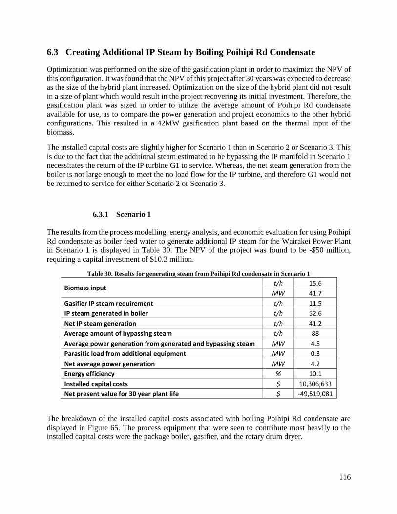
116
6.3 Creating Additional IP Steam by Boiling Poihipi Rd Condensate
Optimization was performed on the size of the gasification plant in order to maximize the NPV of
this configuration. It was found that the NPV of this project after 30 years was expected to decrease
as the size of the hybrid plant increased. Optimization on the size of the hybrid plant did not result
in a size of plant which would result in the project recovering its initial investment. Therefore, the
gasification plant was sized in order to utilize the average amount of Poihipi Rd condensate
available for use, as to compare the power generation and project economics to the other hybrid
configurations. This resulted in a 42MW gasification plant based on the thermal input of the
biomass.
The installed capital costs are slightly higher for Scenario 1 than in Scenario 2 or Scenario 3. This
is due to the fact that the additional steam estimated to be bypassing the IP manifold in Scenario 1
necessitates the return of the IP turbine G1 to service. Whereas, the net steam generation from the
boiler is not large enough to meet the no load flow for the IP turbine, and therefore G1 would not
be returned to service for either Scenario 2 or Scenario 3.
6.3.1 Scenario 1
The results from the process modelling, energy analysis, and economic evaluation for using Poihipi
Rd condensate as boiler feed water to generate additional IP steam for the Wairakei Power Plant
in Scenario 1 is displayed in Table 30. The NPV of the project was found to be -$50 million,
requiring a capital investment of $10.3 million.
Table 30. Results for generating steam from Poihipi Rd condensate in Scenario 1
Biomass input t/h 15.6
MW 41.7
Gasifier IP steam requirement t/h 11.5
IP steam generated in boiler t/h 52.6
Net IP steam generation t/h 41.2
Average amount of bypassing steam t/h 88
Average power generation from generated and bypassing steam MW 4.5
Parasitic load from additional equipment MW 0.3
Net average power generation MW 4.2
Energy efficiency % 10.1
Installed capital costs $ 10,306,633
Net present value for 30 year plant life $ -49,519,081
The breakdown of the installed capital costs associated with boiling Poihipi Rd condensate are
displayed in Figure 65. The process equipment that were seen to contribute most heavily to the
installed capital costs were the package boiler, gasifier, and the rotary drum dryer.

117
Figure 65. The installed cost breakdown for using Poihipi Rd condensate as boiler feed water in Scenario 1
The cumulative discounted cash flows for this project is displayed in Figure 66. It can be seen that
the implementation of the hybrid configuration does not generate yearly profit, with the estimated
cost for the landing residues being greater than the estimated value of the additional power
generated.
Figure 66. The cumulative discounted cash flow for using Poihipi Rd condensate as boiler feed water in
Scenario 1
A summary of the cash flows for the implantation of this project is displayed in Table 31.

118
Table 31. The cash flow summary for using Poihipi Rd condensate as boiler feed water n Scenario 1, all
values given in $1000’s
Year Capital
Cost Revenue
Operating costs
Cost of biomass
Income tax
Free Cash flow
0 -888 0 0 0 0 -888 1 -9419 0 0 0 0 -9419 2 0 2649 -108 -6135 1031 -2563 3 0 2728 -111 -6250 1066 -2567 4 0 2828 -114 -6368 1072 -2582 5 0 2897 -1053 -6488 1349 -3295 6 0 2969 -204 -6611 1126 -2720 7 0 3046 -210 -6736 1141 -2759
8 0 3127 -216 -6864 1156 -2797 9 0 3182 -223 -6994 1179 -2856
10 0 3149 -1900 -7127 1694 -4182 20 0 3432 -2553 -8612 2214 -5519 30 0 3890 -3431 -10428 2840 -7129
The sensitivity analysis for this project is displayed in Figure 67. The sale price of power and the
cost of the landing residues were seen to have the greatest influence on the NPV of the project.
However, within the ±30% sensitivity range chosen for this analysis, none of the manipulated
factors resulted in the project recovering its initial investment.
Figure 67. Sensitivity analysis for using Poihipi Rd condensate as boiler feed water in Scenario 1
6.3.2 Scenario 2
The results from the process modelling, energy analysis, and economic evaluation for using Poihipi
Rd condensate as boiler feed water to generate additional IP steam for the Wairakei Power Plant

119
in Scenario 2 is displayed in Table 32. The NPV for the 30 year plant life of the hybrid
configuration was calculated as -$62 million, and requires a $9.6 million capital investment.
Table 32. Results for generating steam from Poihipi Rd condensate in Scenario 2
Biomass input t/h 15.6
MW 41.7
Gasifier IP steam requirement t/h 11.5
IP steam generated in boiler t/h 52.7
Net IP steam generation t/h 41.2
Average power generation from generated steam MW 2.0
Parasitic load from additional equipment MW 0.3
Net average power generation MW 1.7
Energy efficiency % 4.1
Installed capital costs $ 9,546,633
Net present value for 30 year plant life $ -62,138,611
The breakdown of the installed capital costs is displayed in Figure 68. There is no cost associated
with returning steam turbines to service, as all of the steam generated in the boiler is only used in
the LP turbine G7, which is already in service.
Figure 68. The installed capital cost breakdown for using Poihipi Rd condensate as boiler feed water in
Scenario 2
The cumulative discounted cash flows for this project are displayed in Figure 69. Similar to in
Scenario 1, the project is not expected to become revenue positive at any point in the life of the
hybrid plant.

120
Figure 69. The cumulative discounted cash flow for using Poihipi Rd condensate as boiler feed water in
Scenario 2
A summary of the cash flows for the implantation of this project is displayed in Table 33.
Table 33. The cash flow summary for using Poihipi Rd condensate as boiler feed water n Scenario 2, all
values given in $1000’s
Year Capital
Cost Revenue
Operating costs
Cost of biomass
Income tax
Free Cash flow
0 -888 0 0 0 0 -888 1 -8659 0 0 0 0 -8659 2 0 1063 -34 -6135 1451 -3656 3 0 1095 -35 -6250 1495 -3696 4 0 1135 -36 -6368 1517 -3752 5 0 1162 -118 -6488 1566 -3878 6 0 1191 -121 -6611 1593 -3948 7 0 1222 -125 -6736 1621 -4018 8 0 1255 -128 -6864 1648 -4089 9 0 1277 -132 -6994 1680 -4170
10 0 1264 -815 -7127 1912 -4766 20 0 1377 -1095 -8612 2374 -5956 30 0 1561 -1472 -10428 2937 -7402
The sensitivity analysis from Scenario 2 is displayed in Figure 70. The reduced power generation
for this configuration in Scenario 2 causes the value for the price of power to have a smaller impact
on the NPV of the project than in the other scenarios.

121
Figure 70. Sensitivity analysis for using Poihipi Rd condensate as boiler feed water in Scenario 2
6.3.3 Scenario 3
The results from the process modelling, energy analysis, and economic evaluation for using Poihipi
Rd condensate as boiler feed water to generate additional IP steam for the Wairakei Power Plant
in Scenario 3 is displayed in Table 34. The NPV of this project was found to be -$32 million for
the 30 year plant life, and required a $9.6 million investment.
Table 34. Results for generating steam from Poihipi Rd condensate in Scenario 1
Biomass input t/h 15.6
MW 41.7
Gasifier IP steam requirement t/h 11.5
IP steam generated in boiler t/h 52.7
Net IP steam generation t/h 41.2
Average power generation from generated steam MW 6.5
Parasitic load from additional equipment MW 0.3
Net average power generation MW 6.2
Energy efficiency % 14.8
Installed capital costs $ 9,546,633
Net present value for 30 year plant life $ -32,281,561
The installed capital costs and the distribution of the installed costs is the same in Scenario 3 as in
Scenario 2, and therefore, the capital cost breakdown can be seen in Figure 68.
The cumulative discounted cash flows for this project can be seen in Figure 71. Though Scenario
3 resulted in the highest NPV of the three scenarios for this configuration, the additional power
generation was not sufficient to result in the project becoming revenue positive at any point in the
hybrid plants operation.

122
Figure 71. The cumulative discounted cash flow for using Poihipi Rd condensate as boiler feed water in
Scenario 3
A summary of the cash flows for the implantation of this project is displayed in Table 35.
Table 35. The cash flow summary for using Poihipi Rd condensate as boiler feed water n Scenario 3, all
values given in $1000’s
Year Capital
Cost Revenue
Operating costs
Cost of biomass
Income tax
Free Cash flow
0 -888 0 0 0 0 -888 1 -8659 0 0 0 0 -8659 2 0 3895 -34 -6135 658 -1616 3 0 4012 -35 -6250 678 -1595 4 0 4159 -36 -6368 671 -1575 5 0 4260 -37 -6488 676 -1589 6 0 4367 -38 -6611 681 -1602 7 0 4480 -39 -6736 685 -1611 8 0 4599 -41 -6864 687 -1618 9 0 4680 -42 -6994 701 -1654
10 0 4632 -43 -7127 753 -1786 20 0 5047 -58 -8612 1056 -2567 30 0 5721 -78 -10428 1382 -3404
The sensitivity analysis for this project is displayed in Figure 72. The relatively large amount of
power generated for this configuration in Scenario 3 served to increase the sensitivity of the NPV
of the project to the price of power.
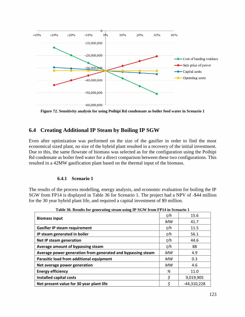
123
Figure 72. Sensitivity analysis for using Poihipi Rd condensate as boiler feed water in Scenario 1
6.4 Creating Additional IP Steam by Boiling IP SGW
Even after optimization was performed on the size of the gasifier in order to find the most
economical sized plant, no size of the hybrid plant resulted in a recovery of the initial investment.
Due to this, the same flowrate of biomass was selected as for the configuration using the Poihipi
Rd condensate as boiler feed water for a direct comparison between these two configurations. This
resulted in a 42MW gasification plant based on the thermal input of the biomass.
6.4.1 Scenario 1
The results of the process modelling, energy analysis, and economic evaluation for boiling the IP
SGW from FP14 is displayed in Table 36 for Scenario 1. The project had a NPV of -$44 million
for the 30 year hybrid plant life, and required a capital investment of $9 million.
Table 36. Results for generating steam using IP SGW from FP14 in Scenario 1
Biomass input t/h 15.6
MW 41.7
Gasifier IP steam requirement t/h 11.5
IP steam generated in boiler t/h 56.1
Net IP steam generation t/h 44.6
Average amount of bypassing steam t/h 88
Average power generation from generated and bypassing steam MW 4.9
Parasitic load from additional equipment MW 0.3
Net average power generation MW 4.6
Energy efficiency % 11.0
Installed capital costs $ 9,019,905
Net present value for 30 year plant life $ -44,310,228

124
The breakdown of the installed capital costs for this project is displayed in Figure 73. The boiler,
dryer, and gasifier were seen to be the most expensive pieced of equipment.
Figure 73. The breakdown of the installed capital costs for using IP SGW from FP14 to generate additional
steam in Scenario 1
The cumulative discounted cash flow for generating additional steam from FP14 IP SGW is
displayed in Figure 74. As can be seen, this configuration does not become revenue positive over
the 30 year life of the hybrid plant.

125
Figure 74. The cumulative discounted cash flows for generating additional steam by boiling IP SGW from
FP14 in Scenario 1
A summary of the cash flows for the implantation of this project is displayed in Table 37.
Table 37. The cash flow summary for boiling IP SGW from FP14 in Scenario 1, all values given in $1000’s
Year Capital
Cost Income
Operating costs
Cost of biomass
Income tax
Free Cash flow
0 -814 0 0 0 0 -814 1 -8206 0 0 0 0 -8206 2 0 2883 -74 -6135 955 -2371 3 0 2970 -76 -6250 987 -2370 4 0 3078 -78 -6368 990 -2378 5 0 3153 -161 -6488 1026 -2470 6 0 3232 -166 -6611 1040 -2505 7 0 3316 -171 -6736 1053 -2538 8 0 3404 -176 -6864 1065 -2571 9 0 3464 -181 -6994 1086 -2625
10 0 3428 -865 -7127 1325 -3239
20 0 3735 -1849 -8612 1930 -4795 30 0 4234 -3224 -10428 2684 -6734
The sensitivity analysis for this project is displayed in Figure 75. This project was seen to be
relatively insensitive to manipulations of the capital and operating costs, as these were relatively
small compared to the cost of landing residues, and the value of the additional power generated.

126
Figure 75. Sensitivity analysis for generating additional steam fusing IP SGW from FP14 as feed water in
Scenario 1
6.4.2 Scenario 2
The results of the process modelling, energy analysis, and economic evaluation for boiling the IP
SGW from FP14 is displayed in Table 38 for Scenario 2. The NPV of the project was found to be
-$58 million for the 30 year hybrid plant life, and required a capital investment of $8.3 million.
Table 38. Results for generating steam using IP SGW from FP14 in Scenario 2
Biomass input t/h 15.6
MW 41.7
Gasifier IP steam requirement t/h 11.5
IP steam generated in boiler t/h 56.1
Net IP steam generation t/h 44.6
Average power generation from generated steam MW 2.3
Parasitic load from additional equipment MW 0.3
Net average power generation MW 2.0
Energy efficiency % 4.8
Installed capital costs $ 8,259,905
Net present value for 30 year plant life $ -58,950,702
The breakdown of the installed capital costs is displayed in Figure 76. There was a reduction in
the capital costs for this configuration in Scenario 2 compared to Scenario 1, as the boiler did not
generated additional IP steam sufficient to justify the return of the IP turbine G1 to service.
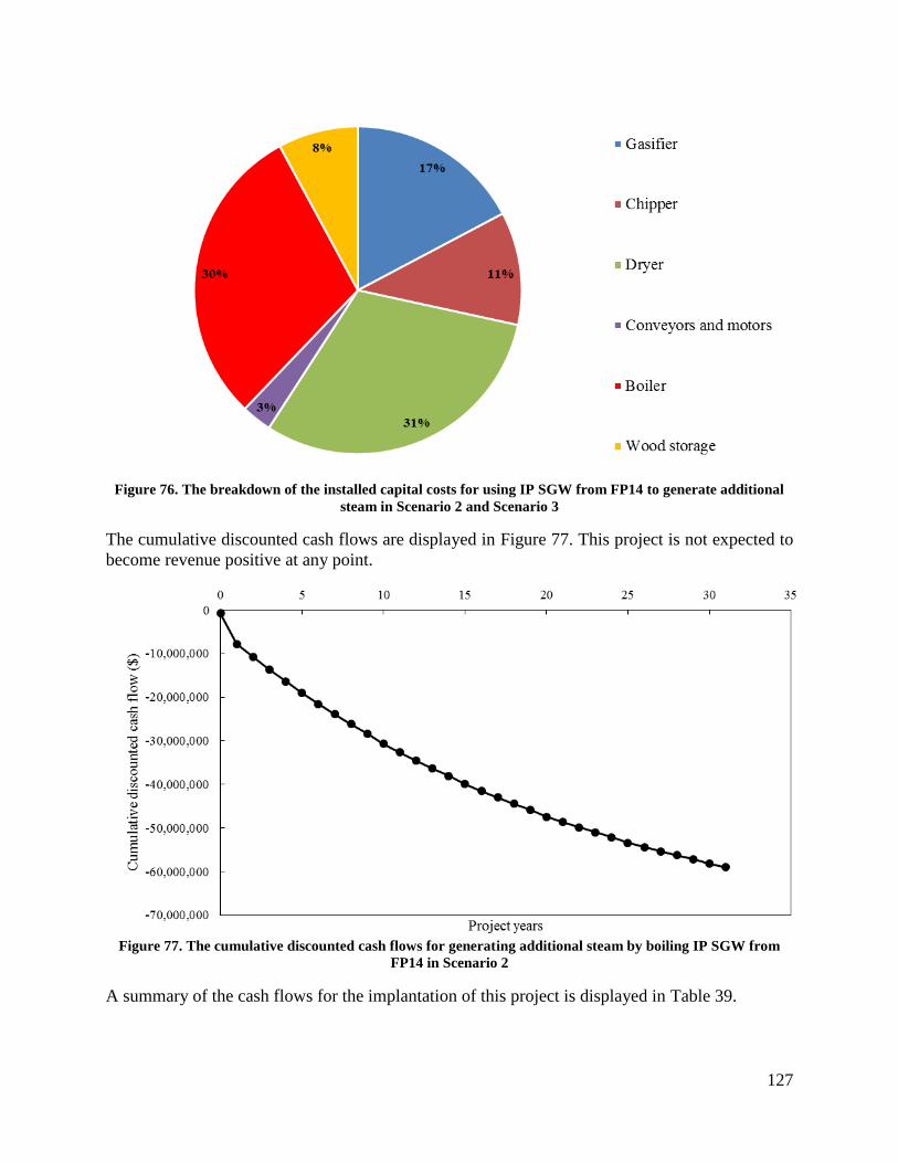
127
Figure 76. The breakdown of the installed capital costs for using IP SGW from FP14 to generate additional
steam in Scenario 2 and Scenario 3
The cumulative discounted cash flows are displayed in Figure 77. This project is not expected to
become revenue positive at any point.
Figure 77. The cumulative discounted cash flows for generating additional steam by boiling IP SGW from
FP14 in Scenario 2
A summary of the cash flows for the implantation of this project is displayed in Table 39.
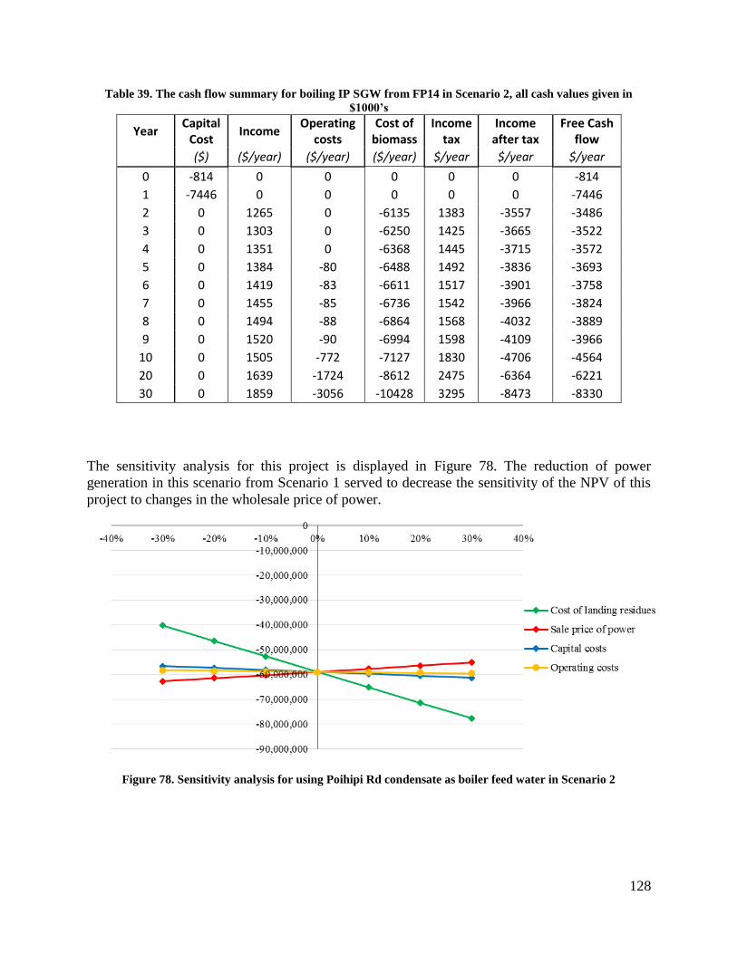
128
Table 39. The cash flow summary for boiling IP SGW from FP14 in Scenario 2, all cash values given in
$1000’s
Year Capital
Cost Income
Operating costs
Cost of biomass
Income tax
Income after tax
Free Cash flow
($) ($/year) ($/year) ($/year) $/year $/year $/year
0 -814 0 0 0 0 0 -814 1 -7446 0 0 0 0 0 -7446 2 0 1265 0 -6135 1383 -3557 -3486 3 0 1303 0 -6250 1425 -3665 -3522 4 0 1351 0 -6368 1445 -3715 -3572 5 0 1384 -80 -6488 1492 -3836 -3693 6 0 1419 -83 -6611 1517 -3901 -3758
7 0 1455 -85 -6736 1542 -3966 -3824 8 0 1494 -88 -6864 1568 -4032 -3889
9 0 1520 -90 -6994 1598 -4109 -3966 10 0 1505 -772 -7127 1830 -4706 -4564 20 0 1639 -1724 -8612 2475 -6364 -6221 30 0 1859 -3056 -10428 3295 -8473 -8330
The sensitivity analysis for this project is displayed in Figure 78. The reduction of power
generation in this scenario from Scenario 1 served to decrease the sensitivity of the NPV of this
project to changes in the wholesale price of power.
Figure 78. Sensitivity analysis for using Poihipi Rd condensate as boiler feed water in Scenario 2

129
6.4.3 Scenario 3
The results of the process modelling, energy analysis, and economic evaluation for boiling the IP
SGW from FP14 is displayed in Table 40 for Scenario 3. This project was found to have a NPV
of -$27 million, and requires a capital investment of $8.3 million.
Table 40. Results for generating steam using IP SGW from FP14 in Scenario 3
Biomass input t/h 15.6
MW 41.7
Gasifier IP steam requirement t/h 11.5
IP steam generated in boiler t/h 56.1
Net IP steam generation t/h 44.6
Average power generation from generated steam MW 7.1
Parasitic load from additional equipment MW 0.3
Net average power generation MW 6.8
Energy efficiency % 16.2
Installed capital costs $ 8,259,905
Net present value for 30 year plant life $ -27,232,629
The same process equipment is required in this scenario as in Scenario 2, the cost breakdown is
therefore displayed in Figure 76.
The cumulative discounted cash flows are displayed in Figure 79. Similar to the other steam flow
scenarios, this configuration is not expected to become revenue positive at any point in the hybrid
plants operation.
Figure 79. The cumulative discounted cash flows for generating additional steam by boiling IP SGW from
FP14 in Scenario 3
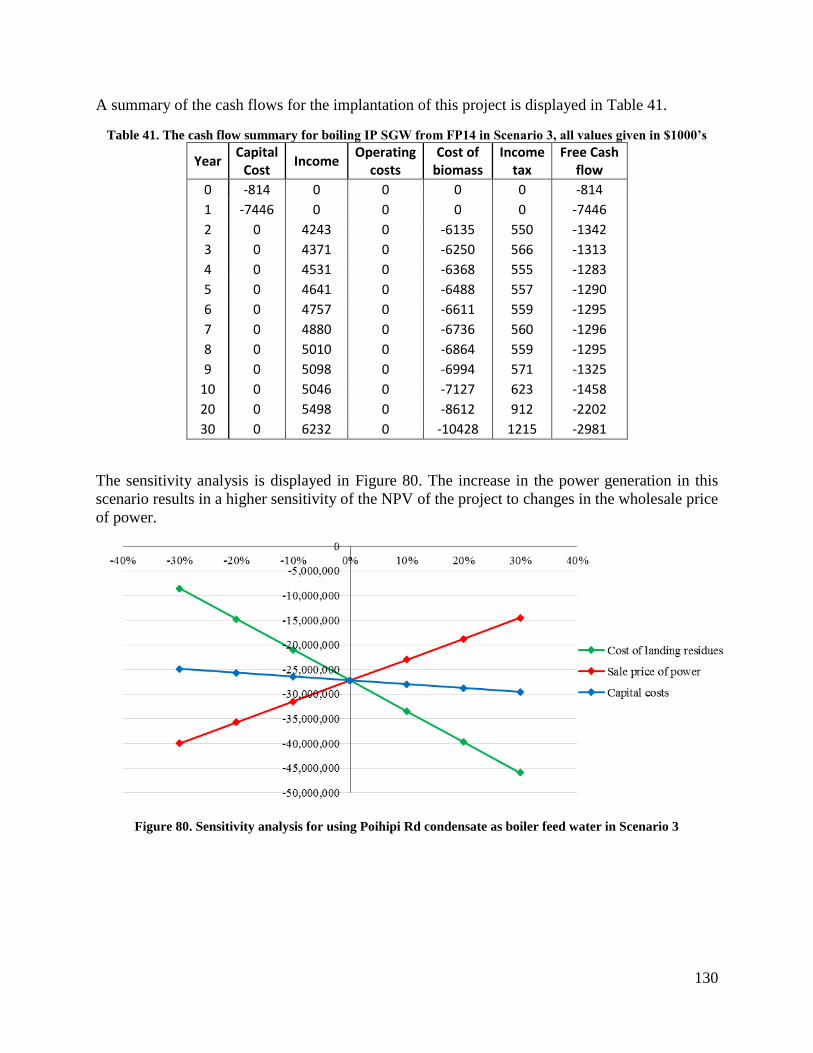
130
A summary of the cash flows for the implantation of this project is displayed in Table 41.
Table 41. The cash flow summary for boiling IP SGW from FP14 in Scenario 3, all values given in $1000’s
Year Capital
Cost Income
Operating costs
Cost of biomass
Income tax
Free Cash flow
0 -814 0 0 0 0 -814 1 -7446 0 0 0 0 -7446 2 0 4243 0 -6135 550 -1342 3 0 4371 0 -6250 566 -1313 4 0 4531 0 -6368 555 -1283 5 0 4641 0 -6488 557 -1290 6 0 4757 0 -6611 559 -1295
7 0 4880 0 -6736 560 -1296 8 0 5010 0 -6864 559 -1295 9 0 5098 0 -6994 571 -1325
10 0 5046 0 -7127 623 -1458 20 0 5498 0 -8612 912 -2202 30 0 6232 0 -10428 1215 -2981
The sensitivity analysis is displayed in Figure 80. The increase in the power generation in this
scenario results in a higher sensitivity of the NPV of the project to changes in the wholesale price
of power.
Figure 80. Sensitivity analysis for using Poihipi Rd condensate as boiler feed water in Scenario 3

131
6.5 Heating Additional SGW to Utilize in the Binary Plant
Optimization was performed to fins the most economic sized gasification plant to heat and supply
additional SGW to the Wairakei Binary Plant. However, as for the other configurations, it was
found that there was no limit on the SGW that would result in a recovery of the capital investment
for the hybrid configuration after 30 years. Therefore, in order to compare the two applicable
scenarios for this configuration, it was assumed that there would be no limit on the amount of
SGW to be heated other than those associated with the amount available for use in T-line, and the
maximum of 2800 t/h for the total SGW flow to the Wairakei Binary Plant. This configuration was
only evaluated for Scenario 1 and Scenario 2, as this configuration does not produce additional
steam, and therefore the unused capacity of the Wairakei steam turbines has no effect on the power
generation or plant economics of this configuration.
6.5.1 Scenario 1
The results of the process modelling, energy analysis, and economic evaluation for heating SGW
to generate additional power from the Binary Plant is displayed in Table 42 for Scenario 1. This
project resulted in an NPV of -$17 million for the 30 year life of the hybrid plant, and required a
$7.8 million capital investment.
Table 42. Results for generating additional power by heating makeup SGW for the Binary Plant for Scenario
1
Average biomass input t/h 3.4
MW 9.3
Maximum biomass input t/h 6.2
MW 16.2
Average IP steam requirement for the gasifier t/h 2.5
Power loss from gasifier steam use MW 0.22
Average SGW added to the Binary Plant t/h 267
Average additional power generation from the Binary Plant MW 1.75
Parasitic load from additional equipment MW 0.3
Net average power generation MW 1.43
Average energy efficiency % 15.5
Installed capital costs $ 7,767,617
Net present value for 30 year plant life $ -17,133,272
The breakdown of the installed capital costs is displayed in Figure 81. As can be seen, the furnace
is expected to be the most expensive piece of process equipment.

132
Figure 81. The breakdown of the installed capital costs for generating additional power by heating makeup
SGW for the Binary Plant
The cumulative discounted cash flows are displayed in Figure 82. This project is seen to never
become revenue positive.
Figure 82. The cumulative discounted cash flows for generating additional power by heating makeup SGW
for the Binary Plant for Scenario 1
A summary of the cash flows for the implantation of this project is displayed in Table 43.

133
Table 43. Cash flow analysis for generating additional power by heating makeup SGW for the Binary Plant
in Scenario 1, all values given in $1000’s
Year Capital
Cost Income
Operating costs
Cost of biomass
Income tax
Free Cash flow
0 -723 0 0 0 0 -723 1 -7045 0 0 0 0 -7045 2 0 904 -595 -1219 269 -640 3 0 931 -612 -1242 287 -636 4 0 965 -631 -1265 290 -641 5 0 988 -650 -1289 295 -655 6 0 1013 -669 -1313 300 -669 7 0 1039 -689 -1338 306 -682
8 0 1067 -710 -1363 311 -696 9 0 1086 -731 -1389 319 -716
10 0 1075 -753 -1416 335 -759 20 0 1171 -1012 -1711 464 -1089 30 0 1327 -1360 -2072 618 -1487
The sensitivity analysis is displayed in Figure 83. As can be seen, the NPV of the project is
relatively insensitive to changes in the cost of landing residues, value of power, capital costs, and
operating costs.
Figure 83. Sensitivity analysis for generating additional power by heating makeup SGW for the Binary Plant
for Scenario 1
6.5.2 Scenario 2 & Scenario 3
The results of the process modelling, energy analysis, and economic evaluation for heating SGW
to generate additional power from the Binary Plant is displayed in Table 44 for Scenario 2. This

134
project resulted in a NPV of -$18 million for the 30 year life of the hybrid configuration, and
required a capital investment of $7.8 million.
The steam flow scenario was not seen affect the NPV of the project as strongly as in the other
hybrid configurations. This is due to the additional power generation coming from the binary plant
and not by increasing the steam supply to Wairakei. Therefore only the power losses from steam
used in the biomass gasifier are affected by changes in the steam flow to Wairakei.
Table 44. Results for generating additional power by heating makeup SGW for the Binary Plant for Scenario
2
Average biomass input t/h 3.4
MW 9.3
Average biomass input t/h 6.2
MW 16.2
Average IP steam use by the gasifier t/h 2.5
Power loss from gasifier steam use MW 0.38
Average SGW added to the Binary Plant t/h 267
Average additional power generation from the Binary Plant MW 1.75
Parasitic load from additional equipment MW 0.09
Net average power generation MW 1.28
Average energy efficiency % 13.8
Installed capital costs $ 7,769,678
Net present value for 30 year plant life $ -18,119,856
The breakdown of the installed capital costs is the same for Scenario 2 as it is for Scenario 1, and
is displayed in Figure 81. The cumulative discounted cash flows are displayed in Figure 84.
Figure 84. The cumulative discounted cash flows for generating additional power by heating makeup SGW
for the Binary Plant for Scenario 2
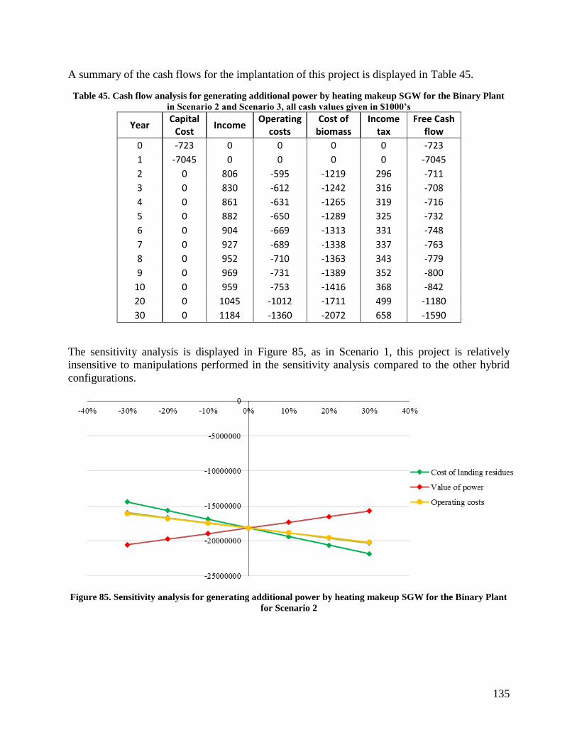
135
A summary of the cash flows for the implantation of this project is displayed in Table 45.
Table 45. Cash flow analysis for generating additional power by heating makeup SGW for the Binary Plant
in Scenario 2 and Scenario 3, all cash values given in $1000’s
Year Capital
Cost Income
Operating costs
Cost of biomass
Income tax
Free Cash flow
0 -723 0 0 0 0 -723 1 -7045 0 0 0 0 -7045 2 0 806 -595 -1219 296 -711 3 0 830 -612 -1242 316 -708 4 0 861 -631 -1265 319 -716 5 0 882 -650 -1289 325 -732
6 0 904 -669 -1313 331 -748 7 0 927 -689 -1338 337 -763 8 0 952 -710 -1363 343 -779
9 0 969 -731 -1389 352 -800 10 0 959 -753 -1416 368 -842 20 0 1045 -1012 -1711 499 -1180 30 0 1184 -1360 -2072 658 -1590
The sensitivity analysis is displayed in Figure 85, as in Scenario 1, this project is relatively
insensitive to manipulations performed in the sensitivity analysis compared to the other hybrid
configurations.
Figure 85. Sensitivity analysis for generating additional power by heating makeup SGW for the Binary Plant
for Scenario 2

136
6.6 Discussion
6.6.1 Biomass Gasification
The cold gas efficiency of the dual fluidized bed gasifier is seen to be relatively high compared to
other gasifiers of the same type, due to the use of geothermal IP steam in the DFB gasifier. This
high efficiency indicates that the integration of geothermal and gasification technologies may be a
viable method to increase the efficiency of biomass gasifiers using steam as the gasification agent.
However, this cold gas efficiency does not take into account the loss of power generation caused
by the reduction of steam input to the steam turbines. While this is taken into account in the overall
biomass-electricity efficiencies for the plant configurations, the cold gas efficiencies of 79-84%
do not accurately represent all of the inputs for gasification. By using the enthalpy of the IP steam,
at 2.744 MJ/kg, the cold gas efficiency of the gasifier drops to 69% in the superheating geothermal
steam configuration, and 65% in all other configurations. This is a more accurate representation of
the actual performance of the gasifier, and is within the expected range for cold gas efficiencies
given by Devi, Ptasinski, and Janssen, of 60-70% [98].
The dual fluidized bed (DFB) gasifier was selected for this project, due in part to the experience
that the Department of Chemical and Process Engineering at the University of Canterbury has with
using this type of gasifier. This allowed use of sophisticated heat and material models for biomass
gasification, which would have been outside the scope of this project to create. However, as a
major advantage of the DFB gasifier is the ability to create energy dense syngas which may be
used to synthesize liquid fuels, it may be more favourable to use a different type of gasifier. An air
blown gasifier produces less energy dense syngas, but would remove the need to utilize geothermal
IP steam in the gasifier. However, the subsequent energy requirement for blowers or compressors
for the air input to the gasifier, and the lower flame temperature from the dilute syngas may limit
any benefits from using an air blown gasifier.
6.6.2 Hybrid Power Plant Energy Efficiency
The energy efficiency of the hybrid plants was seen to be highly dependent on the amount of steam
input to the Wairakei Power Plant. The presence of the bypassing IP steam in Scenario 1 served to
increase the efficiency of every configuration. However, the configurations creating additional IP
steam supply to Wairakei were seen to be the most efficient when the steam could be used in
partially loaded turbines as in Scenario 3. The uncertainty associated with estimating the amount
of steam input to Wairakei therefore has a corresponding uncertainty in the potential energy
efficiency of the different hybrid configurations.
The net steam production in the hybrid configurations is also seen to greatly impact the plant
efficiency. The no load flow of the steam turbines is seen to greatly impact the power generation
capacity of the produced steam, as more steam is produced, the proportion required to satisfy the
no load flow requirement decreases. This is of specific importance for the configuration boiling
Poihipi Rd condensate, as there is a maximum of 54 t/h of condensate available, the resultant IP
steam generation would not be large enough to satisfy the no load flow requirement for an unloaded
137
IP turbines. Therefore, there is an associated decrease of the power generation ability of the steam
as it is throttled down to LP.
Due to the availability of bypassing steam in Scenario 1, additional power generation is possible
without the implementation of a biomass gasifier if the IP steam turbine G1 is returned to service.
Due to this, the energy efficiency of configurations that return the IP turbine G1 to service is seen
to decrease as the size of the gasification plant increases. However, the method used to estimate
the bypassing steam has a relatively large uncertainty associated with it, due to the accuracy of the
steam flow measurements to Wairakei. Also, the elimination of the negative results for the
expected bypassing steam may serve to overestimate the bypassing steam, as it reduced the effect
of negatively deviated estimates but did not remove positively deviated estimates.
The superheating of the geothermal steam was found to have largest energy efficiency of the hybrid
configurations. This configuration in Scenario 3 attained a comparable power generation
efficiency to those for gasification gas engine and syngas combustion and steam generation power
plants at similar plant sizes [99] However, the relatively high energy efficiency that was attained
by this configuration in Scenario 3, at 29%, however requires very specific steam flows to
Wairakei. Scenario 3 assumes that the steam flow to Wairakei has decreased to the point where
the IP turbine G4 is partially loaded. There is a saving of 138 t/h of IP steam by modifying two of
the MP turbines and the full load capacity of G4 is 241 t/h, 100 t/h of which is the no load flow
requirement. Therefore there would need to be a geothermal steam flow to G4 within 100 – 103
t/h in order for the all additional IP steam to be utilized in G4 without contributing to the no load
flow of the turbine. This range is broader for the configurations implementing a boiler, as they
generate significantly less steam than is saved in the superheated geothermal steam configuration.
While each steam flow scenario was created to estimate the efficiencies of the hybrid plant
configurations, they also show how the performance of these plants is expected to change
throughout their life. As the steam flow to Wairakei is expected to decrease in coming years, there
could be a continuous progression of the performance of the hybrid plants from Scenario 1 through
Scenario 2 to Scenario 3, and potentially further into steam flow cases that were not investigated.
However, with decreasing steam flow to Wairakei, steam turbines will be removed from service
essentially reverting the case to one similar to Scenario 1, where the remaining turbines are fully
loaded, and there is sporadic bypassing of additional steam.
The decreasing enthalpy of the geothermal reservoir may also serve to increase the SGW loading
of the Wairakei Binary Plant without hybridization. As more SGW will be produced from the
lower enthalpy two-phase fluid extracted from the reservoir, flow of SGW to the binary plant is
likely to increase.
Typical power generation efficiencies for a gasification combustion and steam cycle plants are
approximately 20% for a 10 MWe plant size [100]. This is seen to be higher than almost all of the
hybrid configurations. It would be expected that a hybrid geothermal/gasification plant would have
a higher efficiency than a gasification power plant [25]. As the gasifier cold gas efficiency is
relatively high; the relatively low power generation efficiencies are therefore attributed to the
design constraints associated with retrofitting the gasifier to an existing power plant.

138
6.6.3 Hybrid Power Plant Economic Assessment
The results from the economic assessment do not appear to be promising for the financial viability
of any of the hybrid configurations. None of the hybrid configurations are seen to recover the
initial capital investment from the hybridization of the Wairakei Geothermal System with a
biomass gasifier. Only one configuration, the superheating of geothermal steam, is seen to be cash
flow positive in any of the 30 years lives of the proposed hybrid plants, and this only occurs in
Scenario 3, where the steam may be used in partially loaded IP and LP turbines, and this required
specific steam flows to Wairakei.
There is significant uncertainty associated with some of the estimates for the capital costs for the
implementation of the hybrid configurations, this is most apparent in the rough estimates for the
cost of modifying the MP turbines to utilize superheated steam. The associated costs estimated
from the FACT method may also be an overestimation for some of the process equipment, as these
are estimated purely based on the major equipment costs. These associated costs may
unrealistically inflate the installed cost of process equipment that has a large equipment cost, such
as if expensive materials were used in the construction. The cost estimates for the minor materials,
such as piping and electrical, at 60% of the major equipment cost, while potentially valid for the
construction of new process plants, is likely an overestimation in this case; as the majority of the
piping and electrical infrastructure required for the hybrid configurations is already present on the
Wairakei site. However, as only the superheating of geothermal steam was seen to be cash flow
positive, and this only in specific circumstances; the capital costs of the hybrid configurations is
not seen to be the main factor which causes the retrofitting of the Wairakei Geothermal System
with biomass gasification to be financially impractical.
The factors which were seen to consistently have the greatest impact on the NPV of the hybrid
configurations were the price of electricity, and the cost of the landing residues. As estimates for
the price of electricity were based on those used by Contact Energy, it is unlikely that, barring
large disruption of the electricity market, these would have an associated uncertainty large enough
to cause the hybrid configurations to become prudent investments. However, there is significant
uncertainty attached to the estimation of the prices for the landing residues. As landing residues
are not a commonly sold good, there is very little information for the expected cost of the landing
residues. The price estimates were entirely based on those reported by Scion in their report on
bioenergy options in New Zealand [66]. The method for inflating the cost of the landing residues
based on the historical costs for pulp logs, while imperfect, will likely not misrepresent the
inflation of the landing residues to the degree that would be required for any of the hybrid
configurations to be economically viable. Similarly, it is unlikely that the wiggle factor used to
increase the straight line distance to a more accurate travel distance would have an associated
uncertainty large enough to cause any of the configurations to be economically viable. Therefore
the cost of landing residues reported by Scion would need to significantly overestimate the true
costs for delivered landing residues in order for retrofitting a biomass gasifier to become a prudent
investment. The analysis performed into the expected cost of landing residues and the wholesale
price of power also forecasted the price of the landing residues to increase at a greater rate than
the value of power. This served to decrease the free cash flow of the hybrid configurations
throughout the operational life of the hybrid plants.

139
As the performance of the biomass gasifier using geothermal IP steam as the gasification agent
was seen to be relatively good, the inefficiencies associated with retrofitting syngas use into an
existing geothermal power plant served to limit the power production, and therefore the economics
of the hybrid plants. It may be possible, instead of using the syngas on site, to sell the syngas
directly as a synthetic natural gas, or to further refine into liquid fuels using Fischer-Tropsch
synthesis for the sale of biofuels. Alternatively, if the hybridization of a biomass gasification and
geothermal steam production could be planned from the design stages of the plant production, it
is likely that higher power generation efficiencies would be attained by removing the design
constraints present when retrofitting an existing geothermal plant with biomass gasification.
6.6.3.1 Breakeven Price of Landing Residues
As the estimated price of landing residues is based on a single report performed by Hall and Gilford
of Scion [66], there is some uncertainty associated with the price of landing residues. The cost of
landing residues that yields a NPV for the hybrid configurations of zero for the 30 year plant life
may be in order to estimate the landing residue costs that would cause the hybrid configurations
to become economically viable. Therefore, if new estimates for the delivered costs of landing
residues become available, the feasibility of the hybrid configuration may be re-evaluated. The
estimated rate of inflation based on the inflation of pulp logs, at approximately 2%, was again used
in order to calculate the initial cost of landing residues which caused the hybrid configurations to
break even. The calculated breakeven prices of landing residues are displayed in Table 46.
Table 46. The breakeven prices of landing residues for the hybrid configurations
Configuration Breakeven Cost of Landing Residues in 2016 ($/GJ)
Scenario 1 Scenario 2 Scenario 3
Superheating Geothermal Steam -0.583 -2.39 2.54
Boiling Poihipi Rd Condensate 0.96 0.01 2.25
Boiling IP SGW from FP14 1.35 0.25 2.63
Heating Additional SGW for Use in the Binary Plant
-1.61 -1.94 -1.94
As can be seen, if landing residues can be obtained for less than approximately $2.50/GJ, some of
the hybrid configurations may recuperate their capital investment over the 30 years of plant
operation. However, as this is only expected to occur in Scenario 3, the uncertainty associated with
the geothermal steam flow to Wairakei is seen to greatly impact the breakeven costs of landing
residues. As the estimated initial costs of landing residues for the hybrid configurations was within
the range of $4-5/GJ, the price of landing residues would have to have been significantly lower
than those estimated in this study in order for the hybrid configurations to become economically
viable.
It is noted that due to the capital investments required, some of the hybrid configurations yielded
negative values for the breakeven costs of landing residues. These configurations would require
payment to receive the landing residues. This is considered to be an unlikely occurrence, as there
is no obvious reason for forestry plantations to pay for landing residues to be removed. However,
it may be possible to identify other types of feedstock, which are waste products, where it may be
possible to receive payment to dispose of the feedstock. Possibilities for this could include
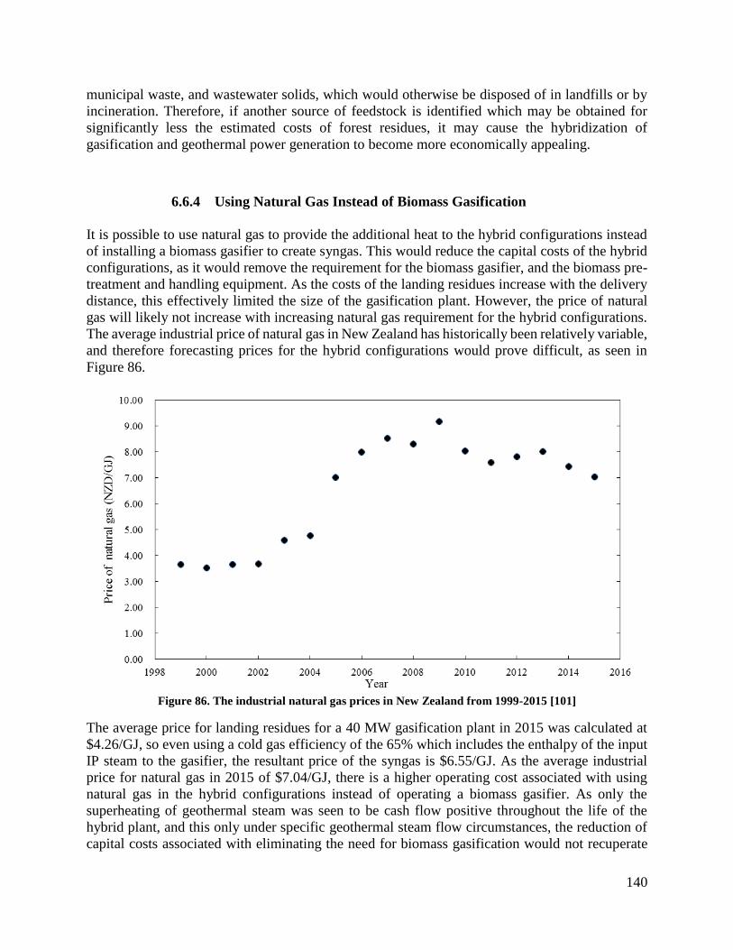
140
municipal waste, and wastewater solids, which would otherwise be disposed of in landfills or by
incineration. Therefore, if another source of feedstock is identified which may be obtained for
significantly less the estimated costs of forest residues, it may cause the hybridization of
gasification and geothermal power generation to become more economically appealing.
6.6.4 Using Natural Gas Instead of Biomass Gasification
It is possible to use natural gas to provide the additional heat to the hybrid configurations instead
of installing a biomass gasifier to create syngas. This would reduce the capital costs of the hybrid
configurations, as it would remove the requirement for the biomass gasifier, and the biomass pre-
treatment and handling equipment. As the costs of the landing residues increase with the delivery
distance, this effectively limited the size of the gasification plant. However, the price of natural
gas will likely not increase with increasing natural gas requirement for the hybrid configurations.
The average industrial price of natural gas in New Zealand has historically been relatively variable,
and therefore forecasting prices for the hybrid configurations would prove difficult, as seen in
Figure 86.
Figure 86. The industrial natural gas prices in New Zealand from 1999-2015 [101]
The average price for landing residues for a 40 MW gasification plant in 2015 was calculated at
$4.26/GJ, so even using a cold gas efficiency of the 65% which includes the enthalpy of the input
IP steam to the gasifier, the resultant price of the syngas is $6.55/GJ. As the average industrial
price for natural gas in 2015 of $7.04/GJ, there is a higher operating cost associated with using
natural gas in the hybrid configurations instead of operating a biomass gasifier. As only the
superheating of geothermal steam was seen to be cash flow positive throughout the life of the
hybrid plant, and this only under specific geothermal steam flow circumstances, the reduction of
capital costs associated with eliminating the need for biomass gasification would not recuperate

141
the capital initial investment for all other configurations. In the superheating geothermal steam
configuration, the biomass gasifier and associated equipment only accounted for $6.2 million, with
the majority of the capital costs coming from the modifications performed on the MP turbines, and
the furnace to superheat the geothermal steam. Comparing this with the cumulative discounted
cash flow displayed in Figure 63, it is clear that this reduction in capital costs would likely not
cause the project to recover its initial investment, especially with the added costs associated with
an increased relative cost of fuel from buying natural gas instead of generating syngas. It is
therefore very unlikely that the use of natural gas as a substitute for biomass gasification without
a significant reduction in the cost of natural gas.
6.6.5 Remaining Life of the Wairakei A and B Stations
The remaining life of the Wairakei A and B Stations may be shorter than the estimated life of the
additional process equipment required for hybridization. Currently, the resource content for the
Wairakei A and B Stations ends in 2026, though this does not necessarily mean that these Power
Stations will be removed from service. There is the possibility of renewing the resource consents
if it is determined that the Wairakei A and B Stations still have remaining useful life. Alternatively,
new power stations could be constructed in order to utilize the geothermal steam which will be
unused in the absence of the Wairakei A and B Stations.
Even if it is decided that the Wairakei A and B Stations should be removed from service, this will
not necessarily remove the possibility of implementing the hybrid configurations. It may be the
case that the modifications performed to the MP turbine(s) in order for it to utilize superheated
steam will increase the useful life of the modified turbines. In both of the configurations utilizing
boilers, it may be that the geothermal steam generated in the boiler can still be utilized at the other
Power Stations on the Wairakei Geothermal Field. However, as these stations are already fully
loaded, the removal of the Wairakei A and B Stations would likely not provide a situation where
there is unused capacity at the Poihipi Rd or Te Mihi Power Stations. Therefore, unless there are
much more strict steam extraction limits put in place on the Wairakei Geothermal Field, which
creates unused capacity at either of these power plants, there would likely be no reason to
implement the hybrid configurations.
As the Wairakei Binary Plant is a relatively recent addition to the Wairakei Geothermal Field, it is
not expected that it would require to be removed from service in the near future. In fact, if the
Wairakei A and B Stations are removed from service, it may be the case that the geothermal steam
used in the biomass gasifier as the gasification agent no longer results in diminished power
generation at these Stations. Currently, this steam use is factored into the net power generation
from the addition of the hybrid configuration to the binary plant. However, if the steam was no
longer to be utilized in steam turbines, then there would be no power losses from using the steam
in the gasifier. This would result in an increase in the net power generation of the Binary Plant.

142
7.0 Conclusions and Recommendations
While investigations have been performed into the possibility of hybridizing geothermal power
plants with additional sources of heating, to this Author’s knowledge this is the first in depth
investigation into retrofitting an existing geothermal steam power plant with additional heating.
Furthermore, using a biomass gasifier to supply the heat to the geothermal power plant is a
desirable first step for the implementation of commercial biomass gasification in New Zealand, as
it would serve to reduce the relative costs of a gasification plant, due to shared equipment.
Four hybrid configurations were designed to produce syngas from biomass combustion in order to
increase the power generation from the geothermal power plants on the Wairakei Geothermal
Field. The water sampling performed showed that the condensate from the Poihipi Rd Power Plant
would likely be suitable as a source of boiler feed water, but would require pH dosing and
deaeration. Three different scenarios were created in order to represent the potential future steam
flows to Wairakei. The process modelling performed on the biomass gasification, Wairakei Power
Station, and the hybrid configurations were created in order to estimate the impact that the different
hybrid configurations would have on the power generation at Wairakei. Plant design and capital
cost estimation was performed in order to determine the investment required in order to implement
the hybrid configurations. An economic evaluation was then performed in order to evaluate the
financial implications of implementing the hybrid configurations.
As the geothermal steam is expected to be used in the biomass gasifier to produce the syngas, and
as the majority of the hybrid configurations provide additional steam to the turbines at Wairakei;
the existing geothermal steam supply to Wairakei has a very large impact on the additional power
that may be generated. The presence of IP steam bypassing the IP and MP turbines to the LP steam
manifold serves to increase the power generation from returning an IP turbine to service, or
mitigate the power losses from using steam in the gasifier. The loading of the steam turbines is
also seen to greatly impact the power generation from the additional steam supply to Wairakei, as
the no load flow requirement for the steam turbines can greatly detract from the amount of steam
that directly contributes to the power generation.
While the superheating of geothermal steam is observed to be the configuration with the highest
energy efficiency, it also is the least flexible of the hybrid configurations. As turbines are required
to be modified, in the event of the closure of the gasifier, there will be a significant impact on the
power generation of the Wairakei A and B Stations. However, this is not the case with the other
configurations, as the existing geothermal power generation is not modified to incorporate the
hybridization.
There is also some uncertainty associated with the practicality of the hybrid configurations. The
superheating of the geothermal steam could cause great damage to the MP turbines, if there are
liquid droplets present in the IP steam feed to the superheater. While it is believed that the operation
of a boiler using the IP SGW and a large blowdown would not result in scaling within the boiler,
the fact remains that the mineral content of the SGW is far greater than would be acceptable in a
conventional boiler. Similarly, as increased mineral scaling has been observed with the mixing of
two sources of SGW, the addition of the heated SGW to the Binary Plant could exacerbate mineral
scaling. Due to the wealth of experience in operating steam boilers, the utilization of the Poihipi

143
Rd condensate as boiler feed water is likely the most practical hybrid configuration. Unfortunately
it also has a relatively low energy efficiency, and requires the addition of several pieces of process
equipment.
It was determined that in all scenarios of future steam flow to Wairakei, none of the hybrid
configurations are expected to recuperate their initial capital investment. Only one configuration
was seen to be cash flow positive during the plant life, and this only in the case of very specific
steam flows to Wairakei. The efficiency losses associated with implementing retrofitted additional
heating in a plant that was only designed to utilize geothermal resources served to significantly
reduce the power generation that may be possible from the hybridization of geothermal and
biomass resources. It was believed that the reduction in capital costs for hybrid geothermal biomass
gasification power plant may cause the implementation of biomass gasification to become
economically feasible. However, it is clear from the yearly losses expected with the
implementation of the hybrid configurations, that the capital costs are not the main barrier to
retrofitting the Wairakei Power Plant with a biomass gasifier.
Overall, and in spite of reasonable solutions to most engineering factors, the limiting factor is the
cost of fuel in the form of the landing residues. It was initially thought that the close proximity and
availability of forestry landing residues would result in viable options for boosting geothermal
power generation via gasification. This is clearly not the case based on the input costs for the
landing residues. The economics would be much more positive if there was a large, reliable and
cheap source of biomass available. Possible situations where this might occur are:
There is a large sawmill adjacent to the geothermal plant and the “waste” from the saw mill
has no other market.
Large quantities of sludge from sewage treatment is readily available. Assuming the sludge
can be delivered with low water content. There is also the possibility of being paid to
dispose of this waste.
Large volumes of biomass from food processing plants have no alternate use.
7.1 Recommendations
7.1.1 Power and Fuel Cogeneration
Due to the limitations imposed by retrofitting an existing geothermal power plant with biomass
gasification in order to generate power, it may be possible to generate syngas to sell as a synthetic
natural gas or further refined into liquid biofuels by Fischer-Tropsch synthesis. As the utilization
of the syngas at Wairakei for power generation was seen to be greatly impacted by the design
constraints of the existing plant, direct sale of the syngas or liquid biofuels may be profitable, as it
would still utilize relatively cheap geothermal steam for the biomass gasification. However, this
would require a significant changes to the gasification design, as impurities in the syngas, such as
tars, would become problematic with the change in use of the syngas. The combustion of syngas
was designed to be used while still at high temperatures in the hybrid configurations, which
avoided the necessity for tar removal, as it would not condense at the elevated temperatures.
144
However, this would not be the case if the syngas was to be sold as a natural gas substitute or used
as an input to Fischer-Tropsch synthesis. It may also be necessary to remove other contaminants
such as chlorides and ammonia from the syngas in order to sell as a natural gas substitute, and
these would certainly be required for liquid synthesis, as there are strict tolerances on the
contaminants in syngas for Fischer-Tropsch synthesis.
The wholesale price of natural gas has been highly variable in New Zealand, which causes
uncertainties in the economic evaluation of a hybrid geothermal/gasification plant which produces
both power and syngas. The average wholesale price of natural gas in 2015 of $5.29/GJ [101] does
not compare particularly favourably with the delivered costs of landing residues as the price of
landing residues for a 40 MW gasification plant was estimated at $4.69/GJ for 2016. Therefore a
gasification plant with a cold gas efficiency of 70%, the cost of biomass to produce 1 GJ of syngas
would be $6.70. Therefore price forecasting for the expected sale price of synthetic natural gas
would be required, in order to evaluate the viability of a hybrid geothermal/gasification power and
syngas cogeneration plant.
The price of liquid fuels is seen to be more stable than that of natural gas in New Zealand, and
therefore the price forecasting for liquid biofuels should prove to be simpler than for natural gas.
The smallest cost for liquid fuels reported by the Ministry of Business Innovation and Employment
for heavy fuel oil was seen to have an average price of $12.40/GJ in 2015[101]. Integration of
liquid biofuel synthesis to a geothermal power plant may therefore prove to be profitable.
It is recommended that a study into the plant design and market considerations for a
geothermal/gasification power and liquid biofuel cogeneration plant be performed in order to
determine if sale of the syngas will cause hybridization to be economically feasible. It is however
unlikely that a geothermal/gasification power and synthetic natural gas cogeneration plant would
prove to be profitable without a drastic increase in the wholesale price of natural gas.
7.1.2 Further Research into Gasification Feedstocks Prices
Due to the relatively large costs associated with the landing residues estimated in this study, the
economics associated with the hybrid configurations designed in this study were rather pessimistic.
However, due to the fact that only one basis for the cost estimates for landing residues in New
Zealand could be found, it is difficult to verify the validity of these cost estimates. Therefore is
new information is discovered, which suggests that the landing residue costs estimated in this study
are significantly higher than would be expected, it re-evaluation of the feasibility of the hybrid
configurations could be performed. Similarly, if an alternate source of feedstock is identified, it
may cause the economics surrounding biomass gasification retrofitting to a geothermal power
plant to become more promising. This is especially true if a waste product is identified that may
be used as a feedstock to a gasifier, as revenue may be generated by disposing of the feedstock,
instead of paying for it. Possible waste product which may be used as gasification feedstocks are
municipal waste and wastewater solids.
7.1.3 Designing a New Geothermal/Gasification Power Plant

145
By designing a new geothermal/gasification power plant, the limitations associated with
retrofitting an existing geothermal plant with biomass gasification would be removed. More
efficient power generation would be possible in the hybridization occurred from the design stage,
as higher quality steam produced in a boiler or by superheating geothermal steam. This steam
could then be used in new efficient steam turbines designed for the higher quality steam.
Conventional steam power plants create much higher quality steam than the geothermal steam
generated on the Wairakei Geothermal System to generate power, due to the greater efficiency that
is possible by using superheated steam. The desired reduction in the relative costs of the biomass
gasifier and associated equipment would still be achieved through shared equipment with the
geothermal portion of the plant. Due to this, it is suggested that hybridization of geothermal and
gasification power generation be researched for a new hybrid power plant. As Contact Energy has
resource consents to construct a new geothermal power station on the Wairakei Geothermal field,
the Tauhara II Power Station, it may be possible to integrate biomass gasification into the design
of this power plant.
146
8.0 References
1. REN21, Renewables 2014 Global Status Report. 2014.
2. U.S., CHINA RATIFY PARIS CLIMATE AGREEMENT. 2016 7 Sep 2016]; Available from:
http://www.reuters.com/article/us-china-climatechange-idUSKCN11901W?il=0.
3. Modelling Electricity Demand in New Zealand - overview guide. 2014, New Zealand Electricity
Authority.
4. Gray, J., Mighty River Battles Flat Demand, in NZ Herald. 2014.
5. New Zealand Ministry of Buisness Innovation & Employment, Energy in New Zealand. 2015.
6. DiPippo, R., Part 1 - Resource Identification and Development, in Geothermal Power Plants
(Second Edition), R. DiPippo, Editor. 2008, Butterworth-Heinemann: Oxford. p. 1-2.
7. DiPippo, R., Chapter 7 - Dry-Steam Power Plants, in Geothermal Power Plants (Second Edition),
R. DiPippo, Editor. 2008, Butterworth-Heinemann: Oxford. p. 135-156.
8. Appendix A - Worldwide State of Geothermal Power Plant Development as of May 2007, in
Geothermal Power Plants (Second Edition), R. DiPippo, Editor. 2008, Butterworth-Heinemann:
Oxford. p. 413-432.
9. Thain, I.A. and B. Carey, Fifty years of geothermal power generation at Wairakei. Geothermics,
2009. 38(1): p. 48-63.
10. DiPippo, R., Chapter 5 - Single-Flash Steam Power Plants, in Geothermal Power Plants (Second
Edition), R. DiPippo, Editor. 2008, Butterworth-Heinemann: Oxford. p. 81-112.
11. E.W. Lemmon, M.O.M.a.D.G.F., Thermophysical Properties of Fluid Systems, in NIST Chemistry
WebBook. National Institute of Standards and Technology.
12. Schlömer S., T.B., L. Fulton, E. Hertwich, A. McKinnon, D. Perczyk, J. Roy, R. Schaeffer, R.
Sims, P. Smith, and R. Wiser, Annex III: Technology-specific cost and performance parameters.
In: Climate Change 2014: Mitigation of Climate Change. Contribution of Working Group III to
the Fifth Assessment Report of the Intergovernmental Panel on Climate Change. 2014, Cambridge
University Press, Cambridge, United Kingdom and New York, NY, USA.
13. DiPippo, R., Chapter 8 - Binary Cycle Power Plants, in Geothermal Power Plants (Second
Edition), R. DiPippo, Editor. 2008, Butterworth-Heinemann: Oxford. p. 157-189.
14. New Zealand Geothermal Association. Price 7/5/2016]; Available from:
http://www.nzgeothermal.org.nz/price.html.
15. Higman, C. and M. van der Burgt, Chapter 1 - Introduction, in Gasification (Second Edition), C.
Higman and M.v.d. Burgt, Editors. 2008, Gulf Professional Publishing: Burlington. p. 1-9.
16. Higman, C. and M. van der Burgt, Chapter 4 - Feedstocks and Feedstock Characteristics, in
Gasification (Second Edition), C. Higman and M.v.d. Burgt, Editors. 2008, Gulf Professional
Publishing: Burlington. p. 47-90.
17. Basu, P., Chapter 8 - Biomass Handling, in Biomass Gasification and Pyrolysis, P. Basu, Editor.
2010, Academic Press: Boston. p. 269-299.
18. Gopalakrishnan, P., Modelling of Biomass Steam Gasification in a Bubbling Fluidized Bed
Gasifier, in Chemical and Process Engineering. 2013, University of Canterbury.
19. Basu, P., Chapter 6 - Design of Biomass Gasifiers, in Biomass Gasification and Pyrolysis, P. Basu,
Editor. 2010, Academic Press: Boston. p. 167-228.
20. Williamson, C., Liquid Fuel from Biomass Derived Synthesis Gas via Fischer-Tropsch
[PowerPoint slides]. Department of Chemical & Process Engineering, University of Canterbury.
21. Roberts, K., Diagrams of the Wairakei Geothermal Field. 2015, Contact Energy.
22. White, B., Wairakei Energy and Efficiency Audit. 2000, PARSONS BRINCKERHOFF.

147
23. Dowell, M. Te Mihi Geothermal Power Station. 10/05/2016]; An overview of the work that the
McConnell Dowell Contruction Company performed constructing the Te Mihi Power Station].
Available from: www.mccinnelldowell.com/markets/power/100-te-mihi-geothermal-power-
station.
24. Zarrouk, S.J., B.C. Woodhurst, and C. Morris, Silica scaling in geothermal heat exchangers and
its impact on pressure drop and performance: Wairakei binary plant, New Zealand. Geothermics,
2014. 51(0): p. 445-459.
25. DiPippo, R., Chapter 9 - Advanced Geothermal Energy Conversion Systems, in Geothermal Power
Plants (Third Edition), R. DiPippo, Editor. 2012, Butterworth-Heinemann: Boston. p. 183-221.
26. DiPippo, R. Geothermal electric power production in the United States: a survey and update for
1990–1994. in Proceedings of the World Geothermal Congress. 1995.
27. Tanaka, Y., et al., Performance of a Hybrid Power Generation System Using Biomass Gasification
and Concentrated Solar Thermal Processes. Energy Procedia, 2014. 61(0): p. 2149-2153.
28. Horlock, J.H., Combined Power Plants : Including Combined Cycle Gas Turbine (CCGT) Plants.
Thermodynamics and fluid mechanics series. 1992, Oxford [England] ; New York Pergamon Press.
29. Bixley, P.F., A.W. Clotworthy, and W.I. Mannington, Evolution of the Wairakei geothermal
reservoir during 50 years of production. Geothermics, 2009. 38(1): p. 145-154.
30. Kristmannsdóttir, H. and H. Ármannsson, Environmental aspects of geothermal energy utilization.
Geothermics, 2003. 32(4–6): p. 451-461.
31. Kingston Reynolds Thom and Allardice Ltd, An Investigation into Hybrid Geothermal/Gas Power
Plants. 1980, New Zealand Energy Research and Development Committee.
32. Ian Thain, R.D., Hybrid Geothermal-Biomass Power Plants: Applications, Designs and
Performance Analysis, in World Geothermal Congress 2015. 2015: Melbourne, Australia.
33. Rosalind Julian, K.L., Geothermal Materials Selection in Old Lessons, New Directions, N.Z.G.
Association, Editor. 2014, Quest Integrity Group.
34. Woolcock, P.J. and R.C. Brown, A review of cleaning technologies for biomass-derived syngas.
Biomass and Bioenergy, 2013. 52(0): p. 54-84.
35. Baratieri, M., et al., The use of biomass syngas in IC engines and CCGT plants: A comparative
analysis. Applied Thermal Engineering, 2009. 29(16): p. 3309-3318.
36. Brown, R.C. and T.R. Brown, Biorenewable resources: engineering new products from
agriculture. 2013: John Wiley & Sons.
37. Ronald DiPippo, H.E.K., Robert J. Correia and Joseph Kestin, Fossil Superheating in Geothermal
Steam Power Plants. 1978, Brown University: Providence, Rhode island.
38. Morris, C., Superheating Steam for a Geothermal Turbine. 2014.
39. Kennedy, G.C., A portion of the system silica-water. Economic Geology and the Bulletin of the
Society of Economic Geologists, 1950: p. 629-653.
40. Rayaprolu, K., Boilers: A Practical Reference, C. Press, Editor. 2012.
41. Gallup, D.L., J.L. Featherstone, and C.E. Flint, Use of steam condensate to dilute brine stream
additives. 1995, Google Patents.
42. Chris Morris, A.R., Geothermal Turbines - A Maintainer's Perspective, in World Geothermal
Congress. 2015: Melbourne, Australia.
43. Puladian, N., Development of an integrated system model for production of fischer-tropsch liquid
fuels from woody biomass, in Department of Chemical and Process Engineering. 2015, University
of Canterbury: Christchurch, New Zealand.
44. Iguaz, A., et al., Mathematical modelling and simulation for the drying process of vegetable
wholesale by-products in a rotary dryer. Journal of food engineering, 2003. 59(2): p. 151-160.
45. Xu, Q. and S. Pang, Mathematical modeling of rotary drying of woody biomass. Drying
Technology, 2008. 26(11): p. 1344-1350.
46. Amos, W.A., Report on Biomass Drying Technology. 1998, National Renewable Energy
Laboratory: Colorado, U.S.A.

148
47. Fagbemi, L., L. Khezami, and R. Capart, Pyrolysis products from different biomasses: Application
to the thermal cracking of tar. Applied Energy, 2001. 69(4): p. 293-306.
48. Koppatz, S., C. Pfeifer, and H. Hofbauer, Comparison of the performance behaviour of silica sand
and olivine in a dual fluidised bed reactor system for steam gasification of biomass at pilot plant
scale. Chemical Engineering Journal, 2011. 175: p. 468-483.
49. Nguyen, T.D.B., et al., Three-stage steady-state model for biomass gasification in a dual
circulating fluidized-bed. Energy Conversion and Management, 2012. 54(1): p. 100-112.
50. The Engineering Toolbox. Butterfly Valves - Typical Flow Coefficients. [cited 2016 11/7].
51. Sarco, S., Steam Sizing Chart. Spirax Sarco.
52. Brooks, C., Boiler Efficiency Guide, C. Brooks, Editor. 2010: USA.
53. Saidur, R., J.U. Ahamed, and H.H. Masjuki, Energy, exergy and economic analysis of industrial
boilers. Energy Policy, 2010. 38(5): p. 2188-2197.
54. Davis, J.R., ASM specialty handbook: heat-resistant materials. 1997: Asm International.
55. Gary Eng, I.B., Charles Hendtlass, New Zealand Energy Information Handbook. 2008, New
Zealand Centre for Advanced Engineering: Christchurch.
56. Muller, L., Water Analysis at Wairakei, S. Chester, Editor. 2015.
57. Electric, G., Handbook of Industrial Water Treatment. GE Water
58. Fegley Jr, B., et al., Solubility of Rock in Steam Atmospheres of Planets. arXiv preprint
arXiv:1602.00658, 2016.
59. Millero, F.J., The effect of pressure on the solubility of minerals in water and seawater. Geochimica
et Cosmochimica Acta, 1982. 46(1): p. 11-22.
60. Federation, W.E. and A.P.H. Association, Standard methods for the examination of water and
wastewater. American Public Health Association (APHA): Washington, DC, USA, 2005.
61. Heselton, K.E., Boiler operator's handbook. 2005: The Fairmont Press, Inc.
62. American Boiler Manufacturers Association, Deaerator White Paper for use with
Industrial/Commercial and Institutional Boilers. 2011.
63. Branan, C.R., Rules of thumb for chemical engineers. 2012: Butterworth-Heinemann.
64. North Carolina Department of Environment and Natural Resources, Boiler Blowdown Fact Sheet.
2004.
65. Reserve Bank of New Zealand. Inflation Calculator. 2016; Available from:
http://www.rbnz.govt.nz/monetary-policy/inflation-calculator.
66. Peter Hall, J.G., Bioenergy Options for New Zealand, A Situation Analysis of Biomass Resources
and Conversion Technologies, M. Richardson, Editor. 2007, Scion, Energy Group.
67. New Zealand Ministry of Primary Industries. Indicative New Zealand Radiata Pine Log Prices by
Quarter. 2016 [cited 2016 25/7/2016]; Available from: http://www.mpi.govt.nz/news-and-
resources/open-data-and-forecasting/forestry/indicative-new-zealand-radiata-pine-log-prices-by-
quarter/.
68. New Zealand Ministry of Primary Industries, Indicative New Zealand Radiata Pine Log Prices by
Quarter. 2016.
69. Sherwin, A., National Exotic Forest Description. 2014, Ministry for Primary Industries:
Wellington, New Zealand.
70. Domínguez-Caamaño, P., J.A.C. Benavides, and J.C.P. Prado, AN IMPROVED METHODOLOGY
TO DETERMINE THE WIGGLE FACTOR: AN APPLICATION FOR SPANISH ROAD
TRANSPORT. Brazilian Journal of Operations & Production Management, 2016. 1(1): p. 52-56.
71. Society of Chemical Engineers New Zealand, Cost Estimating by the FACT Method. 2004.
72. van der Drift, A., J. van Doorn, and J.W. Vermeulen, Ten residual biomass fuels for circulating
fluidized-bed gasification. Biomass and Bioenergy, 2001. 20(1): p. 45-56.
73. Hakkila, P., Utilization of residual forest biomass. 1989: Springer.
74. Naimi, L.J., et al. Cost and performance of woody biomass size reduction for energy production.
in 2006 ASAE Annual Meeting. 2006. American Society of Agricultural and Biological Engineers.

149
75. Goho, C.D., A study of logging residue at woods landings in Appalachia. Vol. 219. 1976: US Dept.
of Agriculture, Forest Service, Northeastern Forest Experiment Station.
76. Merat, M.S., Contact Energy, Wairakei, NZ- Disc Chipper for Chipping Residues and Logs up to
500mm dia, up to m metres long, S. Chester, Editor. 2016: Southern Cross Engineering.
77. Holmberg, H. and P. Ahtila, Evaluation of energy efficiency in biofuel drying by means of energy
and exergy analyses. Applied Thermal Engineering, 2005. 25(17–18): p. 3115-3128.
78. Ruiz, J.A., et al., Biomass gasification for electricity generation: Review of current technology
barriers. Renewable and Sustainable Energy Reviews, 2013. 18: p. 174-183.
79. Brammer, J.G. and A.V. Bridgwater, Drying technologies for an integrated gasification bio-energy
plant. Renewable and Sustainable Energy Reviews, 1999. 3(4): p. 243-289.
80. Penniall, C.L. and C.J. Williamson, Feasibility study into the potential for gasification plant in the
New Zealand wood processing industry. Energy Policy, 2009. 37(9): p. 3377-3386.
81. Brammer, J.G. and A.V. Bridgwater, The influence of feedstock drying on the performance and
economics of a biomass gasifier–engine CHP system. Biomass and Bioenergy, 2002. 22(4): p. 271-
281.
82. Worley, M. and J. Yale, Biomass Gasification Technology Assessment: Consolidated Report. 2012,
National Renewable Energy Laboratory (NREL), Golden, CO.
83. Woodenergy Wood Fuel Characteristics.
84. K.C. Dhuyvetter, J.P.H., III, G. Boomer, J.F. Smith, R. Rodriguez, Bunkers, piles, or bags: Which
is most economical? Western Dairy News, 2006. 6(1).
85. University of Georgia, C.o.A.E.S., Extension Engineering Handbook. University of Georgia.
86. Henan Province Yingda Machinery Manufacturing Co., L. Wood chips auger conveyor with
capacity 18t/h. [cited 2016 17/05]; Details on wood chip transfer augers ]. Available from:
https://www.alibaba.com/product-detail/Wood-chips-auger-conveyor-with-
capacity_60242259797.html?spm=a2700.7724857.29.84.QwY13y.
87. Henan Wantai Machinery Co., L. Wood Chip Conveyor. [cited 2016 19/05].
88. Rutherford, J.P., Heat and Power Applications of Advanced Biomass Gasifiers in New Zealand's
Wood Industry A Chemical Equilibrium Model and Economic Feasibility Assessment, in Chemical
and Process Engineering. 2006, University of Canterbury.
89. Bhatia, A., Overview of Refractory materials. 2012, PDH Center.
90. Loh, H., J. Lyons, and C. White, Process equipment cost estimation. Final Report, National Energy
Technology Center. 2002, DOE/NETL-2002/1169.
91. Angus, H.T., Cast iron: physical and engineering properties. 2013: Elsevier.
92. Galu, N., Cost of caustic soda, S. Chester, Editor. 2016, recochem.com.
93. Wei, S., Quotation of Rotary Dryer, S. Chester, Editor. 2016, ShangHai Tongli Heavy Machinery
Co.: China.
94. Towler, G.P. and R.K. Sinnott, Chemical engineering design: principles, practice and economics
of plant and process design. 2008, Amsterdam;Boston;: Elsevier/Butterworth-Heinemann.
95. Mann, M.K. and P.L. Spath, Life cycle assessment of a biomass gasification combined-cycle power
system. 1997, National Renewable Energy Lab., Golden, CO (US).
96. United States Department of the Treasury Inland Revenue Service, How to Depreciate Properly.
2016.
97. Treasury, N.Z., Public Sector Discount Rates for Cost Benefit Analysis. 2008.
98. Devi, L., K.J. Ptasinski, and F.J.J.G. Janssen, A review of the primary measures for tar elimination
in biomass gasification processes. Biomass and Bioenergy, 2003. 24(2): p. 125-140.
99. Bridgwater, A.V., The technical and economic feasibility of biomass gasification for power
generation. Fuel, 1995. 74(5): p. 631-653.
100. Bridgwater, A., A. Toft, and J. Brammer, A techno-economic comparison of power production by
biomass fast pyrolysis with gasification and combustion. Renewable and Sustainable Energy
Reviews, 2002. 6(3): p. 181-246.

150
101. Ministry of Buisness Innovation & Employment, Energy Prices, in Energy & Building Trends.
2016.

151
9.0 Appendices
9.1 Water testing results
9.1.1 Boiler water testing

152

153

154
9.1.2 Previous Testing Performed on the Poihipi Rd Condensate
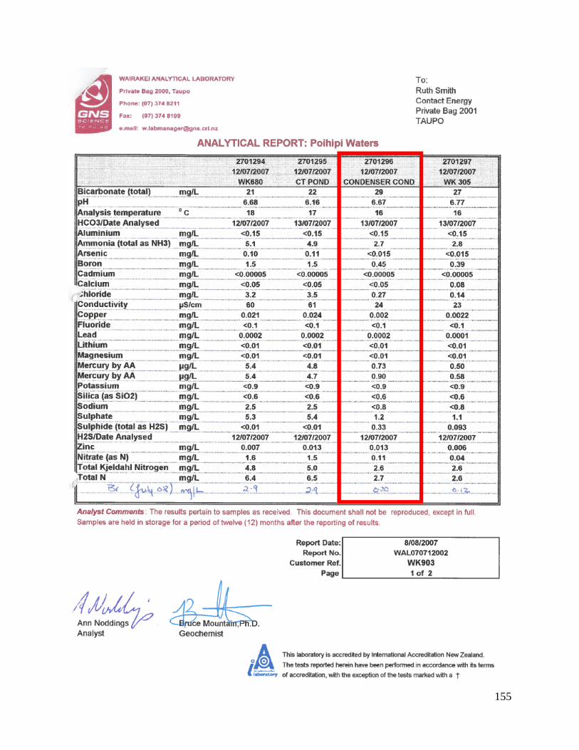
155

156
9.2 Process Equipment Capital Costs
The following tables display to total installed costs for the process equipment required for the
hybrid configurations.
Superheating Geothermal Steam, Scenario 1 & Scenario 2
Process Equipment Total Installed Costs of Process Equipment
Total gasifier cost $ 1,841,853
Chipper $ 920,968
Dryer $ 2,454,390
Conveyors and motors $ 272,479
Wood storage $ 691,855
Furnace $ 9,938,882
Furnace Fan $ 61,244
Cost of modifying MP turbines $ 32,263,262
Cost of bringing IP turbine to service $ 760,000
Total $ 49,204,933
Superheating Geothermal Steam, Scenario 3
Process Equipment Total Installed Costs of Process Equipment
Total gasifier cost $ 1,841,853
Chipper $ 920,968
Dryer $ 2,454,390
Conveyors and motors $ 272,479
Wood storage $ 691,855
Furnace $ 9,938,882
Furnace Fan $ 61,244
Cost of modifying MP turbines $ 32,263,262
Total $ 48,444,933

157
Boiling Poihipi Rd Condensate, Scenario 1
Process Equipment Total Installed Costs of Process Equipment
Total gasifier cost $ 1,889,544.06
Chipper $ 920,967.84
Dryer $ 2,538,220.38
Conveyors and motors $ 272,478.95
Package boiler $ 2,650,829.32
Condensate preheater $ 453,901.46
Wood storage $ 719,976.86
Pumps $ 100,714.86
Cost of Returning IP turbine to Service $ 760,000.00
Total $ 10,306,633.74
Boiling Poihipi Rd Condensate, Scenario 2 & 3
Process Equipment Total Installed Costs of Process Equipment
Total gasifier cost $ 1,889,544
Chipper $ 920,968
Dryer $ 2,538,220
Conveyors and motors $ 272,479
Package boiler $ 2,650,829
Condensate preheater $ 453,901
Wood storage $ 719,977
Pumps $ 100,715
Total $ 9,546,633.74
Boiling IP SGW, Scenario 1
Process Equipment Total Installed Costs of Process Equipment
Total gasifier cost $ 1,425,290
Chipper $ 920,968
Dryer $ 2,538,220
Conveyors and motors $ 247,132
Boiler $ 2,475,293
Wood storage $ 653,002
Returning IP turbine to service $ 760,000
Total $ 9,019,906
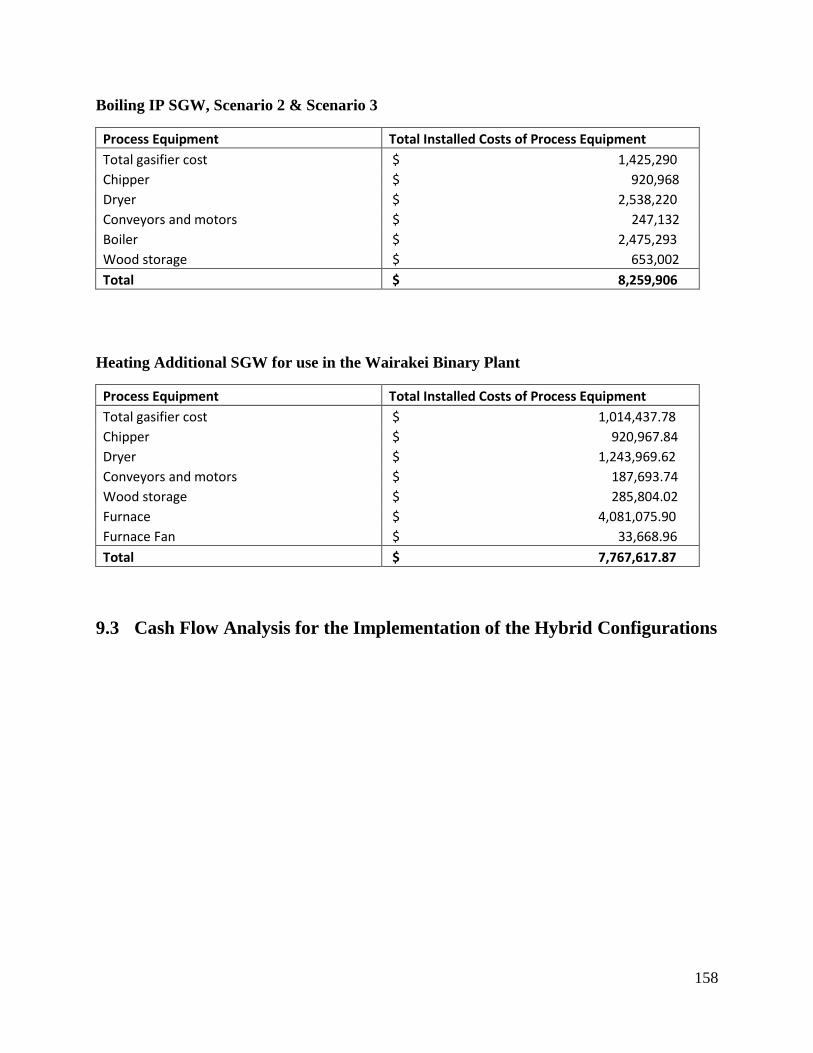
158
Boiling IP SGW, Scenario 2 & Scenario 3
Process Equipment Total Installed Costs of Process Equipment
Total gasifier cost $ 1,425,290
Chipper $ 920,968
Dryer $ 2,538,220
Conveyors and motors $ 247,132
Boiler $ 2,475,293
Wood storage $ 653,002
Total $ 8,259,906
Heating Additional SGW for use in the Wairakei Binary Plant
Process Equipment Total Installed Costs of Process Equipment
Total gasifier cost $ 1,014,437.78
Chipper $ 920,967.84
Dryer $ 1,243,969.62
Conveyors and motors $ 187,693.74
Wood storage $ 285,804.02
Furnace $ 4,081,075.90
Furnace Fan $ 33,668.96
Total $ 7,767,617.87
9.3 Cash Flow Analysis for the Implementation of the Hybrid Configurations

159
Superheating Geothermal Steam, Scenario 1
Year Capital Cost Wholesale
cost of power Average Cost
of wood Sales
Revenue Operating
costs Cost of wood Depreciation
Income tax
Free Cash flow
Discounted Cash Flow (DCF)
Cumulative DCF
($) ($/MWh) ($/GJ) ($/year) ($/year) ($/year) $/year $/year $/year $/year $/year
0 7116274 68.0 4.69 0 0 0 0 0 -7116274 -7116274 -7116274 1 42088659 72.9 4.78 0 0 0 0 0 -42088659 -39335196 -46451469 2 0 75.1 4.87 3970244 75779 5908074 580336 -726305 -1287304 -1124381 -47575851 3 0 77.3 4.96 4089616 78052 6019353 1160324 -887072 -1120717 -914839 -48490689 4 0 80.2 5.05 4239094 80393 6132857 1160324 -877655 -1096502 -836516 -49327206 5 0 82.1 5.15 4342482 1046659 6248634 1160324 -1151678 -1801133 -1284183 -50611389 6 0 84.2 5.25 4450859 170579 6366731 1160324 -909097 -1177354 -784521 -51395909 7 0 86.4 5.35 4566336 175696 6487198 1160324 -911927 -1184631 -737729 -52133638 8 0 88.6 5.45 4687518 180967 6610084 1160324 -913880 -1189653 -692389 -52826027 9 0 90.2 5.55 4770366 186396 6735441 1160324 -927303 -1224169 -665867 -53491893
10 0 89.3 5.66 4720983 1912201 6863321 1160324 -1460162 -2594378 -1318850 -54810743 11 0 91.6 5.76 4841394 197748 6993778 1160324 -982928 -1367204 -649549 -55460292 12 0 90.2 5.87 4771473 203680 7126867 1160324 -1041432 -1517642 -673851 -56134144 13 0 92.3 5.98 4881177 209791 7262643 1160324 -1050443 -1540814 -639383 -56773527 14 0 91.9 6.10 4858860 216084 7401163 1160673 -1097337 -1661051 -644184 -57417711 15 0 93.2 6.22 4929679 2216765 7542486 1160324 -1677171 -3152402 -1142575 -58560286 16 0 93.7 6.33 4953436 229244 7686672 1160673 -1154483 -1807997 -612431 -59172717 17 0 94.1 6.46 4974629 236121 7833782 1160324 -1191568 -1903707 -602665 -59775382 18 0 95.1 6.58 5027059 243205 7983878 1160673 -1220995 -1979029 -585523 -60360905 19 0 94.9 6.71 5019104 250501 8137024 1160324 -1268049 -2100372 -580770 -60941676 20 0 97.3 6.83 5143999 2569838 8293285 1160673 -1926343 -3792782 -980127 -61921803 21 0 100.0 6.97 5289286 265756 8452728 1160324 -1285066 -2144132 -517836 -62439639 22 0 101.2 7.10 5349493 273729 8615421 1160673 -1316092 -2223565 -501888 -62941526 23 0 102.3 7.24 5409700 281941 8781434 1160324 -1347920 -2305755 -486392 -63427918 24 0 103.4 7.38 5469907 290399 8950838 1160673 -1380961 -2390369 -471253 -63899172 25 0 104.6 7.52 5530114 2979147 9123705 1160324 -2165258 -4407481 -812075 -64711246 26 0 105.7 7.66 5590320 308084 9300110 1160673 -1449993 -2567881 -442178 -65153424 27 0 106.9 7.81 5650527 317327 9480130 1160324 -1486031 -2660899 -428219 -65581643 28 0 108.0 7.96 5710734 326847 9663842 1160673 -1523376 -2756579 -414596 -65996239 29 0 109.1 8.12 5770941 336652 9851325 1160324 -1561661 -2855376 -401360 -66397598 30 0 110.3 8.28 5831148 3453648 10042662 1160673 -2471234 -5193928 -682311 -67079910 31 0 111.4 8.44 5891355 357154 10237934 1160324 -1641936 -3061798 -375906 -67455816 32 621764 -174094 174094 19976 -67435840

160
Superheating Geothermal Steam, Scenario 2
Year Capital Cost Wholesale
cost of power Average Cost
of wood Sales
Revenue Operating
costs Cost of wood Depreciation
Income tax
Free Cash flow
Discounted Cash Flow (DCF)
Cumulative DCF
($) ($/MWh) ($/GJ) ($/year) ($/year) ($/year) $/year $/year $/year $/year $/year
0 7116274 68.0 4.69 0 0 0 0 0 -7116274 -7116274 -7116274 1 42088659 72.9 4.78 0 0 0 0 0 -42088659 -39335196 -46451469 2 0 75.1 4.87 1662464 75779 5870887 580336 -1362071 -2922131 -2552302 -49003772 3 0 77.3 4.96 1712449 78052 5981465 1160324 -1542070 -2804998 -2289714 -51293486 4 0 80.2 5.05 1775040 80393 6094256 1160324 -1556781 -2842828 -2168780 -53462266 5 0 82.1 5.15 1818331 1046659 6209304 1160324 -1847428 -3590204 -2559766 -56022031 6 0 84.2 5.25 1863712 170579 6326658 1160324 -1622278 -3011247 -2006521 -58028552 7 0 86.4 5.35 1912066 175696 6446367 1160324 -1643690 -3066307 -1909542 -59938094 8 0 88.6 5.45 1962809 180967 6568480 1160324 -1665150 -3121489 -1816735 -61754829 9 0 90.2 5.55 1997500 186396 6693048 1160324 -1691835 -3190109 -1735208 -63490037
10 0 89.3 5.66 1976822 1912201 6820124 1160324 -2216432 -4539072 -2307434 -65797471 11 0 91.6 5.76 2027241 197748 6949760 1160324 -1758565 -3361701 -1597120 -67394591 12 0 90.2 5.87 1997963 203680 7082011 1160324 -1805455 -3482273 -1546171 -68940762 13 0 92.3 5.98 2043900 209791 7216933 1160324 -1832082 -3550742 -1473432 -70414194 14 0 91.9 6.10 2034555 216084 7354582 1160673 -1875099 -3661012 -1419803 -71833997 15 0 93.2 6.22 2064209 2216765 7495016 1160324 -2466211 -5181361 -1877964 -73711961 16 0 93.7 6.33 2074157 229244 7638295 1160673 -1947135 -3846247 -1302857 -75014818 17 0 94.1 6.46 2083031 236121 7784479 1160324 -1987410 -3950159 -1250519 -76265337 18 0 95.1 6.58 2104985 243205 7933631 1160673 -2025107 -4046744 -1197286 -77462623 19 0 94.9 6.71 2101654 250501 8085814 1160324 -2070596 -4164065 -1151399 -78614021 20 0 97.3 6.83 2153951 2569838 8241092 1160673 -2748942 -5908036 -1526749 -80140770 21 0 100.0 6.97 2214788 265756 8399532 1160324 -2131031 -4319469 -1043208 -81183979 22 0 101.2 7.10 2239998 273729 8561201 1160673 -2171569 -4423363 -998411 -82182390 23 0 102.3 7.24 2265209 281941 8726169 1160324 -2212903 -4529998 -955589 -83137979 24 0 103.4 7.38 2290419 290399 8894507 1160673 -2255445 -4639043 -914572 -84052551 25 0 104.6 7.52 2315630 2979147 9066287 1160324 -3049236 -6680568 -1230889 -85283440 26 0 105.7 7.66 2340840 308084 9241583 1160673 -2343460 -4865367 -837794 -86121234 27 0 106.9 7.81 2366050 317327 9420470 1160324 -2388980 -4982767 -801878 -86923113 28 0 108.0 7.96 2391261 326847 9603026 1160673 -2435800 -5102813 -767474 -87690587 29 0 109.1 8.12 2416471 336652 9789330 1160324 -2483554 -5225957 -734575 -88425162 30 0 110.3 8.28 2441682 3453648 9979463 1160673 -3402588 -7588841 -996924 -89422086 31 0 111.4 8.44 2466892 357154 10173507 1160324 -2582746 -5481023 -672922 -90095008 32 0 0 0 0 0 0 621764 -174094 174094 19976 -90075032

161
Superheating Geothermal Steam, Scenario 3
Year Capital Cost Wholesale
cost of power Average Cost
of wood Sales
Revenue Operating
costs Cost of wood Depreciation
Income tax
Free Cash flow
Discounted Cash Flow (DCF)
Cumulative DCF
($) ($/MWh) ($/GJ) ($/year) ($/year) ($/year) $/year $/year $/year $/year $/year
0 7116274 68.0 4.69 0 0 0 0 0 -7116274 -7116274 -7116274 1 41328659 72.9 4.78 0 0 0 0 0 -41328659 -38624915 -45741189 2 0 75.1 4.87 7486122 0 5870887 567667 293319 1321917 1154613 -44586576 3 0 77.3 4.96 7711206 0 5981465 1134994 166529 1563211 1276046 -43310530 4 0 80.2 5.05 7993055 0 6094256 1134994 213866 1684934 1285428 -42025102 5 0 82.1 5.15 8187999 0 6209304 1134994 236236 1742458 1242349 -40782753 6 0 84.2 5.25 8392350 0 6326658 1134994 260595 1805096 1202812 -39579941 7 0 86.4 5.35 8610088 0 6446367 1134994 288044 1875678 1168078 -38411864 8 0 88.6 5.45 8838584 0 6568480 1134994 317831 1952273 1136241 -37275623 9 0 90.2 5.55 8994798 0 6693048 1134994 326692 1975058 1074301 -36201322
10 0 89.3 5.66 8901684 0 6820124 1134994 265039 1816521 923427 -35277895 11 0 91.6 5.76 9128726 0 6949760 1134994 292312 1886653 896335 -34381559 12 0 90.2 5.87 8996886 0 7082011 1134994 218367 1696508 753270 -33628290 13 0 92.3 5.98 9203738 0 7216933 1134994 238507 1748298 725481 -32902808 14 0 91.9 6.10 9161659 0 7354582 1135334 188088 1618989 627872 -32274936 15 0 93.2 6.22 9295191 0 7495016 1134994 186251 1613924 584960 -31689976 16 0 93.7 6.33 9339988 0 7638295 1135334 158580 1543112 522706 -31167270 17 0 94.1 6.46 9379948 0 7784479 1134994 128933 1466535 464268 -30703003 18 0 95.1 6.58 9478808 0 7933631 1135334 114756 1430421 423210 -30279793 19 0 94.9 6.71 9463808 0 8085814 1134994 68040 1309954 362213 -29917580 20 0 97.3 6.83 9699304 0 8241092 1135334 90406 1367806 353467 -29564112 21 0 100.0 6.97 9973252 0 8399532 1134994 122844 1450877 350406 -29213707 22 0 101.2 7.10 10086776 0 8561201 1135334 109267 1416307 319679 -28894027 23 0 102.3 7.24 10200299 0 8726169 1134994 94958 1379172 290932 -28603096 24 0 103.4 7.38 10313823 0 8894507 1135334 79515 1339800 264137 -28338958 25 0 104.6 7.52 10427346 0 9066287 1134994 63298 1297761 239111 -28099847 26 0 105.7 7.66 10540869 0 9241583 1135334 45907 1253380 215826 -27884021 27 0 106.9 7.81 10654393 0 9420470 1134994 27700 1206222 194118 -27689903 28 0 108.0 7.96 10767916 0 9603026 1135334 8276 1156614 173957 -27515946 29 0 109.1 8.12 10881440 0 9789330 1134994 -12008 1104117 155198 -27360748 30 0 110.3 8.28 10994963 0 9979463 1135334 -33554 1049054 137811 -27222937 31 0 111.4 8.44 11108487 0 10173507 1134994 -56004 990983 121666 -27101271 32 0 0 0 0 0 0 608190 -170293 170293 19540 -27081731

162
Boiling Poihipi Rd Condensate, Scenario 1
Year Capital Cost Wholesale
cost of power Average Cost
of wood Sales
Revenue Operating
costs Cost of wood Depreciation
Income tax
Free Cash flow
Discounted Cash Flow (DCF)
Cumulative DCF
($) ($/MWh) ($/GJ) ($/year) ($/year) ($/year) $/year $/year $/year $/year $/year
0 888059 68.0 4.71 0 0 0 0 0 -888059 -888059 -888059 1 9418575 72.9 4.80 0 0 0 0 0 -9418575 -8802406 -9690465 2 0 75.1 4.89 2648622 107614 6134838 87399 -1030744 -2563086 -2238699 -11929164 3 0 77.3 4.98 2728257 110843 6250386 174746 -1066161 -2566811 -2095282 -14024446 4 0 80.2 5.07 2827977 114168 6368245 174746 -1072171 -2582265 -1969998 -15994444 5 0 82.1 5.17 2896949 1053373 6488464 174746 -1349497 -3295391 -2349568 -18344012 6 0 84.2 5.26 2969249 203926 6611092 174746 -1125744 -2720025 -1812467 -20156480 7 0 86.4 5.36 3046286 210044 6736180 174746 -1140911 -2759027 -1718183 -21874663 8 0 88.6 5.47 3127129 216345 6863781 174746 -1155768 -2797229 -1628013 -23502676 9 0 90.2 5.57 3182398 222836 6993947 174746 -1178557 -2855828 -1553381 -25056057
10 0 89.3 5.68 3149454 1899630 7126733 174746 -1694464 -4182447 -2126144 -27182201 11 0 91.6 5.78 3229782 236406 7262195 174746 -1244198 -3024621 -1436976 -28619177 12 0 90.2 5.89 3183136 243498 7400389 174746 -1297939 -3162812 -1404326 -30023503 13 0 92.3 6.01 3256322 250803 7541374 174746 -1318968 -3216887 -1334894 -31358397 14 0 91.9 6.12 3241434 258327 7685209 174798 -1365532 -3336570 -1293979 -32652377 15 0 93.2 6.24 3288678 2202192 7831953 174746 -1937660 -4807808 -1742571 -34394947 16 0 93.7 6.36 3304527 274060 7981671 174798 -1435280 -3515923 -1190965 -35585912 17 0 94.1 6.48 3318665 282281 8134424 174746 -1476380 -3621660 -1146525 -36732437 18 0 95.1 6.60 3353643 290750 8290278 174798 -1512611 -3714774 -1099068 -37831504 19 0 94.9 6.73 3348335 299472 8449299 174746 -1561051 -3839385 -1061622 -38893126 20 0 97.3 6.86 3431655 2552944 8611554 174798 -2214140 -5518704 -1426138 -40319264 21 0 100.0 6.99 3528579 317710 8777114 174746 -1607477 -3958768 -956094 -41275359 22 0 101.2 7.12 3568744 327242 8946048 174798 -1646216 -4058329 -916018 -42191377 23 0 102.3 7.26 3608909 337059 9118429 174746 -1685971 -4160608 -877667 -43069044 24 0 103.4 7.40 3649074 347171 9294331 174798 -1726823 -4265604 -840949 -43909994 25 0 104.6 7.54 3689239 2959562 9473829 174746 -2497291 -6246861 -1150979 -45060973 26 0 105.7 7.69 3729404 368313 9657002 174798 -1811798 -4484112 -772144 -45833116 27 0 106.9 7.84 3769570 379363 9843927 174746 -1855970 -4597750 -739918 -46573034 28 0 108.0 7.99 3809735 390743 10034686 174798 -1901338 -4714357 -709050 -47282084 29 0 109.1 8.15 3849900 402466 10229361 174746 -1947868 -4834058 -679489 -47961572 30 0 110.3 8.30 3890065 3430944 10428036 174798 -2840240 -7128675 -936474 -48898046 31 0 111.4 8.47 3930230 426976 10630799 174746 -2044641 -5082904 -624043 -49522089 32 0 0 0 0 0 0 93638 -26219 26219 3008 -49519081

163
Boiling Poihipi Rd Condensate, Scenario 2
Year Capital Cost Wholesale
cost of power Average Cost
of wood Sales
Revenue Operating
costs Cost of wood Depreciation
Income tax
Free Cash flow
Discounted Cash Flow (DCF)
Cumulative DCF
($) ($/MWh) ($/GJ) ($/year) ($/year) ($/year) $/year $/year $/year $/year $/year
0 888059 68.0 4.71 0 0 0 0 0 -888059 -888059 -888059 1 8658575 72.9 4.80 0 0 0 0 0 -8658575 -8092126 -8980185 2 0 75.1 4.89 1062637 34043 6134838 74751 -1450679 -3655565 -3192912 -12173097 3 0 77.3 4.98 1094587 35064 6250386 149457 -1495290 -3695574 -3016689 -15189786 4 0 80.2 5.07 1134595 36116 6368245 149457 -1517383 -3752384 -2862676 -18052462 5 0 82.1 5.17 1162267 117593 6488464 149457 -1566109 -3877681 -2764733 -20817195 6 0 84.2 5.26 1191274 121121 6611092 149457 -1593311 -3947628 -2630471 -23447666 7 0 86.4 5.36 1222181 124754 6736180 149457 -1620699 -4018055 -2502242 -25949909 8 0 88.6 5.47 1254616 128497 6863781 149457 -1648393 -4089269 -2379992 -28329901 9 0 90.2 5.57 1276790 132352 6993947 149457 -1679711 -4169799 -2268094 -30597995
10 0 89.3 5.68 1263572 814805 7126733 149457 -1911678 -4766287 -2422939 -33020934 11 0 91.6 5.78 1295800 140412 7262195 149457 -1751754 -4355053 -2069054 -35089988 12 0 90.2 5.89 1277086 144625 7400389 149457 -1796868 -4471060 -1985204 -37075192 13 0 92.3 6.01 1306448 148963 7541374 149457 -1829337 -4554552 -1889977 -38965170 14 0 91.9 6.12 1300475 153432 7685209 149502 -1872547 -4665619 -1809407 -40774577 15 0 93.2 6.24 1319430 944582 7831953 149457 -2129837 -5327268 -1930847 -42705424 16 0 93.7 6.36 1325789 162776 7981671 149502 -1951085 -4867574 -1648816 -44354240 17 0 94.1 6.48 1331461 167660 8134424 149457 -1993622 -4977001 -1575591 -45929831 18 0 95.1 6.60 1345494 172689 8290278 149502 -2034753 -5082721 -1503794 -47433624 19 0 94.9 6.73 1343365 177870 8449299 149457 -2081313 -5202491 -1438532 -48872157 20 0 97.3 6.86 1376793 1095029 8611554 149502 -2374202 -5955589 -1539037 -50411194 21 0 100.0 6.99 1415679 188702 8777114 149457 -2155886 -5394251 -1302782 -51713976 22 0 101.2 7.12 1431793 194363 8946048 149502 -2200273 -5508344 -1243306 -52957282 23 0 102.3 7.26 1447908 200194 9118429 149457 -2245648 -5625067 -1186590 -54143872 24 0 103.4 7.40 1464022 206200 9294331 149502 -2292083 -5744426 -1132494 -55276366 25 0 104.6 7.54 1480136 1269439 9473829 149457 -2635525 -6627607 -1221131 -56497498 26 0 105.7 7.69 1496251 218758 9657002 149502 -2388123 -5991386 -1031690 -57529187 27 0 106.9 7.84 1512365 225320 9843927 149457 -2437775 -6119107 -984750 -58513937 28 0 108.0 7.99 1528480 232080 10034686 149502 -2488581 -6249705 -939970 -59453907 29 0 109.1 8.15 1544594 239042 10229361 149457 -2540514 -6383295 -897254 -60351161 30 0 110.3 8.30 1560708 1471628 10428036 149502 -2936768 -7402188 -972404 -61323565 31 0 111.4 8.47 1576823 253600 10630799 149457 -2647969 -6659607 -817620 -62141185 32 0 0 0 0 0 0 80087 -22424 22424 2573 -62138612
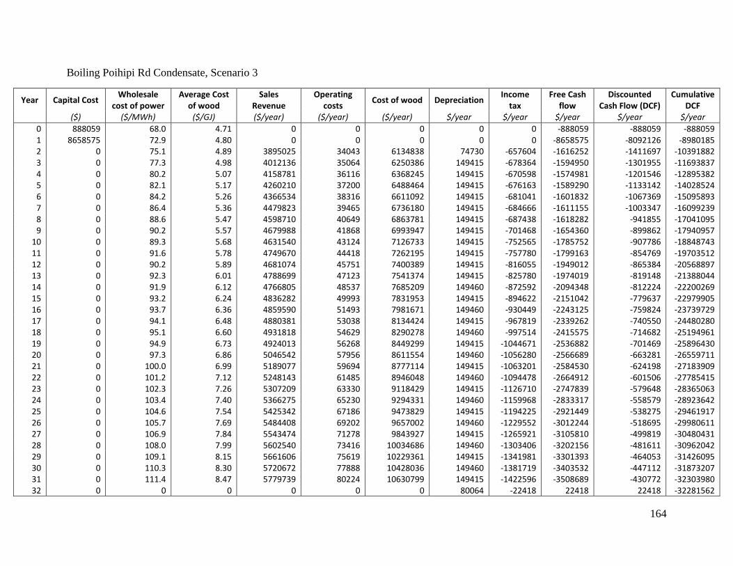
164
Boiling Poihipi Rd Condensate, Scenario 3
Year Capital Cost Wholesale
cost of power Average Cost
of wood Sales
Revenue Operating
costs Cost of wood Depreciation
Income tax
Free Cash flow
Discounted Cash Flow (DCF)
Cumulative DCF
($) ($/MWh) ($/GJ) ($/year) ($/year) ($/year) $/year $/year $/year $/year $/year
0 888059 68.0 4.71 0 0 0 0 0 -888059 -888059 -888059 1 8658575 72.9 4.80 0 0 0 0 0 -8658575 -8092126 -8980185 2 0 75.1 4.89 3895025 34043 6134838 74730 -657604 -1616252 -1411697 -10391882 3 0 77.3 4.98 4012136 35064 6250386 149415 -678364 -1594950 -1301955 -11693837 4 0 80.2 5.07 4158781 36116 6368245 149415 -670598 -1574981 -1201546 -12895382 5 0 82.1 5.17 4260210 37200 6488464 149415 -676163 -1589290 -1133142 -14028524 6 0 84.2 5.26 4366534 38316 6611092 149415 -681041 -1601832 -1067369 -15095893 7 0 86.4 5.36 4479823 39465 6736180 149415 -684666 -1611155 -1003347 -16099239 8 0 88.6 5.47 4598710 40649 6863781 149415 -687438 -1618282 -941855 -17041095 9 0 90.2 5.57 4679988 41868 6993947 149415 -701468 -1654360 -899862 -17940957
10 0 89.3 5.68 4631540 43124 7126733 149415 -752565 -1785752 -907786 -18848743 11 0 91.6 5.78 4749670 44418 7262195 149415 -757780 -1799163 -854769 -19703512 12 0 90.2 5.89 4681074 45751 7400389 149415 -816055 -1949012 -865384 -20568897 13 0 92.3 6.01 4788699 47123 7541374 149415 -825780 -1974019 -819148 -21388044 14 0 91.9 6.12 4766805 48537 7685209 149460 -872592 -2094348 -812224 -22200269 15 0 93.2 6.24 4836282 49993 7831953 149415 -894622 -2151042 -779637 -22979905 16 0 93.7 6.36 4859590 51493 7981671 149460 -930449 -2243125 -759824 -23739729 17 0 94.1 6.48 4880381 53038 8134424 149415 -967819 -2339262 -740550 -24480280 18 0 95.1 6.60 4931818 54629 8290278 149460 -997514 -2415575 -714682 -25194961 19 0 94.9 6.73 4924013 56268 8449299 149415 -1044671 -2536882 -701469 -25896430 20 0 97.3 6.86 5046542 57956 8611554 149460 -1056280 -2566689 -663281 -26559711 21 0 100.0 6.99 5189077 59694 8777114 149415 -1063201 -2584530 -624198 -27183909 22 0 101.2 7.12 5248143 61485 8946048 149460 -1094478 -2664912 -601506 -27785415 23 0 102.3 7.26 5307209 63330 9118429 149415 -1126710 -2747839 -579648 -28365063 24 0 103.4 7.40 5366275 65230 9294331 149460 -1159968 -2833317 -558579 -28923642 25 0 104.6 7.54 5425342 67186 9473829 149415 -1194225 -2921449 -538275 -29461917 26 0 105.7 7.69 5484408 69202 9657002 149460 -1229552 -3012244 -518695 -29980611 27 0 106.9 7.84 5543474 71278 9843927 149415 -1265921 -3105810 -499819 -30480431 28 0 108.0 7.99 5602540 73416 10034686 149460 -1303406 -3202156 -481611 -30962042 29 0 109.1 8.15 5661606 75619 10229361 149415 -1341981 -3301393 -464053 -31426095 30 0 110.3 8.30 5720672 77888 10428036 149460 -1381719 -3403532 -447112 -31873207 31 0 111.4 8.47 5779739 80224 10630799 149415 -1422596 -3508689 -430772 -32303980 32 0 0 0 0 0 0 80064 -22418 22418 22418 -32281562

165
Boiling IPSGW, Scenario 1
Year Capital Cost Wholesale
cost of power Average Cost
of wood Sales
Revenue Operating
costs Cost of wood Depreciation
Income tax
Free Cash flow
Discounted Cash Flow (DCF)
Cumulative DCF
($) ($/MWh) ($/GJ) ($/year) ($/year) ($/year) $/year $/year $/year $/year $/year
0 814166 68.0 4.71 0 0 0 0 0 -814166 -814166 -814166 1 8205740 72.9 4.80 0 0 0 0 0 -8205740 -7668915 -8483082 2 0 75.1 4.89 2883010 73571 6134838 84101 -954660 -2370739 -2070695 -10553777 3 0 77.3 4.98 2969693 75779 6250386 168152 -986895 -2369577 -1934281 -12488057 4 0 80.2 5.07 3078237 78052 6368245 168152 -990139 -2377921 -1814104 -14302162 5 0 82.1 5.17 3153313 160787 6488464 168152 -1025945 -2469993 -1761071 -16063232 6 0 84.2 5.26 3232011 165611 6611092 168152 -1039596 -2505095 -1669251 -17732483 7 0 86.4 5.36 3315865 170579 6736180 168152 -1052533 -2538361 -1580764 -19313246 8 0 88.6 5.47 3403862 175696 6863781 168152 -1065055 -2570560 -1496089 -20809336 9 0 90.2 5.57 3464023 180967 6993947 168152 -1086132 -2624760 -1427695 -22237031
10 0 89.3 5.68 3428163 864878 7126733 168152 -1324848 -3238600 -1646340 -23883371 11 0 91.6 5.78 3515600 191988 7262195 168152 -1149886 -2788697 -1324890 -25208261 12 0 90.2 5.89 3464827 197748 7400389 168152 -1204410 -2928901 -1300467 -26508729 13 0 92.3 6.01 3544488 203680 7541374 168152 -1223241 -2977325 -1235484 -27744213 14 0 91.9 6.12 3528283 209791 7685209 168202 -1269777 -3096939 -1201046 -28945259 15 0 93.2 6.24 3579708 1002631 7831953 168152 -1518448 -3736428 -1354254 -30299512 16 0 93.7 6.36 3596960 222567 7981671 168202 -1337134 -3270143 -1107711 -31407223 17 0 94.1 6.48 3612349 229244 8134424 168152 -1377452 -3373867 -1068080 -32475303 18 0 95.1 6.60 3650421 236121 8290278 168202 -1412370 -3463607 -1024756 -33500059 19 0 94.9 6.73 3644645 243205 8449299 168152 -1460483 -3587376 -991939 -34491999 20 0 97.3 6.86 3735338 1849388 8611554 168202 -1930266 -4795339 -1239207 -35731205 21 0 100.0 6.99 3840839 258016 8777114 168152 -1501484 -3692807 -891861 -36623066 22 0 101.2 7.12 3884558 265756 8946048 168202 -1538726 -3788520 -855119 -37478185 23 0 102.3 7.26 3928278 273729 9118429 168152 -1576969 -3886911 -819932 -38298117 24 0 103.4 7.40 3971997 281941 9294331 168202 -1616294 -3987981 -786217 -39084334 25 0 104.6 7.54 4015717 2439170 9473829 168152 -2258322 -5638961 -1038974 -40123308 26 0 105.7 7.69 4059436 299111 9657002 168202 -1698166 -4198510 -722965 -40846273 27 0 106.9 7.84 4103156 308084 9843927 168152 -1740762 -4308093 -693303 -41539576 28 0 108.0 7.99 4146875 317327 10034686 168202 -1784535 -4420602 -664868 -42204444 29 0 109.1 8.15 4190595 326847 10229361 168152 -1829454 -4536159 -637615 -42842059 30 0 110.3 8.30 4234314 3224421 10428036 168202 -2684177 -6733966 -884622 -43726681 31 0 111.4 8.47 4278034 346752 10630799 168152 -1922947 -4776570 -586434 -44313115 32 0 0 0 0 0 0 90105 -25229 25229 2895 -44310220

166
Boiling IPSGW, Scenario 2
Year Capital Cost Wholesale
cost of power Average Cost
of wood Sales
Revenue Operating
costs Cost of wood Depreciation
Income tax
Free Cash flow
Discounted Cash Flow (DCF)
Cumulative DCF
($) ($/MWh) ($/GJ) ($/year) ($/year) ($/year) $/year $/year $/year $/year $/year
0 814166 68.0 4.71 0 0 0 0 0 -814166 -814166 -814166 1 8205740 72.9 4.80 0 0 0 0 0 -7445740 -6958635 -7772801 2 0 75.1 4.89 1265398 0 6134838 71432 -1383444 -3485996 -3044804 -10817605 3 0 77.3 4.98 1303445 0 6250386 142821 -1425134 -3521808 -2874844 -13692449 4 0 80.2 5.07 1351086 0 6368245 142821 -1444794 -3572364 -2725340 -16417789 5 0 82.1 5.17 1384038 80393 6488464 142821 -1491739 -3693080 -2633115 -19050904 6 0 84.2 5.26 1418580 82805 6611092 142821 -1517079 -3758238 -2504273 -21555177 7 0 86.4 5.36 1455385 85289 6736180 142821 -1542494 -3823591 -2381140 -23936317 8 0 88.6 5.47 1494008 87848 6863781 142821 -1568124 -3889497 -2263723 -26200039 9 0 90.2 5.57 1520414 90484 6993947 142821 -1597915 -3966102 -2157297 -28357336
10 0 89.3 5.68 1504674 771680 7126733 142821 -1830237 -4563502 -2319853 -30677190 11 0 91.6 5.78 1543052 95994 7262195 142821 -1668228 -4146909 -1970167 -32647356 12 0 90.2 5.89 1520766 98874 7400389 142821 -1713969 -4264528 -1893501 -34540858 13 0 92.3 6.01 1555731 101840 7541374 142821 -1744485 -4342998 -1802190 -36343047 14 0 91.9 6.12 1548618 104895 7685209 142864 -1787618 -4453868 -1727287 -38070334 15 0 93.2 6.24 1571190 894589 7831953 142821 -2043489 -5111864 -1852775 -39923109 16 0 93.7 6.36 1578762 111283 7981671 142864 -1863976 -4650217 -1575189 -41498298 17 0 94.1 6.48 1585516 114622 8134424 142821 -1905778 -4757751 -1506182 -43004480 18 0 95.1 6.60 1602227 118061 8290278 142864 -1945713 -4860398 -1438017 -44442497 19 0 94.9 6.73 1599691 121602 8449299 142821 -1991929 -4979281 -1376813 -45819309 20 0 97.3 6.86 1639498 1724138 8611554 142864 -2474936 -6221258 -1607691 -47427001 21 0 100.0 6.99 1685804 129008 8777114 142821 -2061679 -5158639 -1245879 -48672879 22 0 101.2 7.12 1704993 132878 8946048 142864 -2104703 -5269230 -1189334 -49862214 23 0 102.3 7.26 1724182 136865 9118429 142821 -2148701 -5382410 -1135403 -50997617 24 0 103.4 7.40 1743372 140970 9294331 142864 -2193742 -5498187 -1083949 -52081566 25 0 104.6 7.54 1762561 2293971 9473829 142821 -2841457 -7163782 -1319921 -53401487 26 0 105.7 7.69 1781750 149556 9657002 142864 -2286948 -5737859 -988034 -54389520 27 0 106.9 7.84 1800939 154042 9843927 142821 -2335158 -5861872 -943353 -55332873 28 0 108.0 7.99 1820128 158664 10034686 142864 -2384504 -5988717 -900716 -56233589 29 0 109.1 8.15 1839317 163423 10229361 142821 -2434961 -6118506 -860034 -57093624 30 0 110.3 8.30 1858507 3056095 10428036 142864 -3295177 -8330448 -1094347 -58187971 31 0 111.4 8.47 1877696 173376 10630799 142821 -2539404 -6387075 -784160 -58972131 32 0 0 0 0 0 0 76531 -21429 21429 21429 -58950702

167
Boiling IPSGW, Scenario 3
Year Capital Cost Wholesale
cost of power Average Cost
of wood Sales
Revenue Operating
costs Cost of wood Depreciation
Income tax
Free Cash flow
Discounted Cash Flow (DCF)
Cumulative DCF
($) ($/MWh) ($/GJ) ($/year) ($/year) ($/year) $/year $/year $/year $/year $/year
0 814166 68.0 4.71 0 0 0 0 0 -814166 -814166 -814166 1 7445740 72.9 4.80 0 0 0 0 0 -7445740 -6958635 -7772801 2 0 75.1 4.89 4243257 0 6134838 71432 -549644 -1341938 -1172100 -8944902 3 0 77.3 4.98 4370838 0 6250386 142821 -566263 -1313285 -1072032 -10016933 4 0 80.2 5.07 4530594 0 6368245 142821 -554532 -1283119 -978885 -10995818 5 0 82.1 5.17 4641092 0 6488464 142821 -557254 -1290118 -919836 -11915655 6 0 84.2 5.26 4756921 0 6611092 142821 -559158 -1295013 -862922 -12778577 7 0 86.4 5.36 4880339 0 6736180 142821 -559625 -1296216 -807218 -13585795 8 0 88.6 5.47 5009854 0 6863781 142821 -559089 -1294837 -753607 -14339402 9 0 90.2 5.57 5098399 0 6993947 142821 -570744 -1324805 -720606 -15060008
10 0 89.3 5.68 5045620 0 7126733 142821 -622702 -1458412 -741383 -15801390 11 0 91.6 5.78 5174311 0 7262195 142821 -624598 -1463287 -695197 -16496587 12 0 90.2 5.89 5099582 0 7400389 142821 -684216 -1616591 -717786 -17214373 13 0 92.3 6.01 5216829 0 7541374 142821 -690862 -1633682 -677920 -17892293 14 0 91.9 6.12 5192978 0 7685209 142864 -737826 -1754404 -680388 -18572682 15 0 93.2 6.24 5268667 0 7831953 142821 -757710 -1805577 -654424 -19227106 16 0 93.7 6.36 5294058 0 7981671 142864 -792534 -1895079 -641929 -19869035 17 0 94.1 6.48 5316708 0 8134424 142821 -828950 -1988766 -629592 -20498627 18 0 95.1 6.60 5372743 0 8290278 142864 -856912 -2060623 -609664 -21108291 19 0 94.9 6.73 5364241 0 8449299 142821 -903806 -2181252 -603134 -21711425 20 0 97.3 6.86 5497724 0 8611554 142864 -911874 -2201956 -569027 -22280452 21 0 100.0 6.99 5653003 0 8777114 142821 -914741 -2209370 -533592 -22814044 22 0 101.2 7.12 5717350 0 8946048 142864 -944037 -2284661 -515678 -23329722 23 0 102.3 7.26 5781696 0 9118429 142821 -974275 -2362457 -498353 -23828075 24 0 103.4 7.40 5846043 0 9294331 142864 -1005522 -2442765 -481583 -24309658 25 0 104.6 7.54 5910390 0 9473829 142821 -1037753 -2525686 -465356 -24775014 26 0 105.7 7.69 5974737 0 9657002 142864 -1071036 -2611228 -449642 -25224655 27 0 106.9 7.84 6039084 0 9843927 142821 -1105346 -2699497 -434431 -25659086 28 0 108.0 7.99 6103431 0 10034686 142864 -1140753 -2790501 -419698 -26078784 29 0 109.1 8.15 6167778 0 10229361 142821 -1177233 -2884349 -405432 -26484216 30 0 110.3 8.30 6232125 0 10428036 142864 -1214857 -2981054 -391612 -26875829 31 0 111.4 8.47 6296472 0 10630799 142821 -1253601 -3080725 -378230 -27254059 32 0 0 0 0 0 0 76531 -21429 21429 21429 -27232630

168
Heating additional SGW for use in the Wairakei Binary Plant, Scenario 1.
Year Capital Cost Wholesale
cost of power Average Cost
of wood Sales
Revenue Operating
costs Cost of wood
Depreciation Income
tax Free Cash
flow Discounted
Cash Flow (DCF) Cumulative
DCF ($) ($/MWh) ($/GJ) ($/year) ($/year) ($/year) $/year $/year $/year $/year $/year
0 722569 68.0 4.2 0 0 0 -722569 -722569 -722569 1 7045048 72.9 4.3 0 0 0 -7045049 -6584158 -7306727 2 0 75.1 4.3 903710 594547 1218612 51763 -269139 -640310 -559271 -7865998 3 0 77.3 4.4 930882 612384 1241577 103494 -287440 -635638 -518870 -8384868 4 0 80.2 4.5 964906 630755 1265000 103494 -289616 -641233 -489194 -8874061 5 0 82.1 4.6 988440 649678 1288894 103494 -295015 -655117 -467089 -9341151 6 0 84.2 4.7 1013109 669168 1313266 103494 -300390 -668936 -445740 -9786891 7 0 86.4 4.8 1039394 689243 1338127 103494 -305612 -682365 -424943 -10211834 8 0 88.6 4.9 1066977 709921 1363489 103494 -310779 -695653 -404876 -10616710 9 0 90.2 5.0 1085835 731218 1389360 103494 -318707 -716037 -389476 -11006186
10 0 89.3 5.0 1074594 753155 1415752 103494 -335386 -758927 -385800 -11391986 11 0 91.6 5.1 1102002 775749 1442676 103494 -341577 -774846 -368124 -11760110 12 0 90.2 5.2 1086087 799022 1470144 103494 -360241 -822838 -365350 -12125460 13 0 92.3 5.3 1111058 822993 1498167 103494 -367807 -842295 -349522 -12474982 14 0 91.9 5.4 1105978 847682 1526756 103526 -384156 -884304 -342948 -12817931 15 0 93.2 5.5 1122098 873113 1555924 103494 -394921 -912018 -330557 -13148488 16 0 93.7 5.7 1127506 899306 1585683 103526 -409083 -948401 -321256 -13469744 17 0 94.1 5.8 1132329 926285 1616046 103494 -423779 -986223 -312213 -13781957 18 0 95.1 5.9 1144264 954074 1647026 103526 -436901 -1019935 -301762 -14083719 19 0 94.9 6.0 1142453 982696 1678635 103494 -454264 -1064614 -294375 -14378094 20 0 97.3 6.1 1170882 1012177 1710888 103526 -463598 -1088585 -281311 -14659405 21 0 100.0 6.2 1203952 1042542 1743797 103494 -472047 -1110341 -268162 -14927566 22 0 101.2 6.3 1217656 1073819 1777378 103526 -486378 -1147162 -258930 -15186496 23 0 102.3 6.5 1231361 1106033 1811645 103494 -501147 -1185170 -250008 -15436504 24 0 103.4 6.6 1245065 1139214 1846611 103526 -516400 -1224360 -241378 -15677882 25 0 104.6 6.7 1258769 1173391 1882293 103494 -532114 -1264800 -233038 -15910921 26 0 105.7 6.8 1272474 1208592 1918705 103526 -548338 -1306486 -224971 -16135892 27 0 106.9 7.0 1286178 1244850 1955864 103494 -565049 -1349488 -217174 -16353065 28 0 108.0 7.1 1299882 1282196 1993786 103526 -582295 -1393804 -209631 -16562696 29 0 109.1 7.2 1313587 1320661 2032486 103494 -600055 -1439505 -202341 -16765037 30 0 110.3 7.4 1327291 1360281 2071982 103526 -618379 -1486593 -195289 -16960327 31 0 111.4 7.5 1340995 1401090 2112291 103494 -637246 -1535139 -188474 -17148800 32 0 - - - - - 55458 -15528 15528 15528 -17133272

169
Heating additional SGW for use in the Wairakei Binary Plant, Scenarios 2&3
Year Capital Cost Wholesale
cost of power Average Cost
of wood Sales
Revenue Operating
costs Cost of wood
Depreciation Income
tax Free Cash
flow Discounted
Cash Flow (DCF) Cumulative
DCF ($) ($/MWh) ($/GJ) ($/year) ($/year) ($/year) $/year $/year $/year $/year $/year
0 722569 68.0 4.19 0 0 0 0 0 -722569 -722569 -722569 1 7045049 72.9 4.27 0 0 0 0 0 -7045049 -6584158 -7306727 2 0 75.1 4.35 806168 594547 1218612 51763 -296451 -710541 -620614 -7927340 3 0 77.3 4.43 830406 612384 1241577 103494 -315574 -707980 -577923 -8505263 4 0 80.2 4.51 860758 630755 1265000 103494 -318778 -716220 -546401 -9051664 5 0 82.1 4.60 881751 649678 1288894 103494 -324888 -731932 -521857 -9573521 6 0 84.2 4.68 903758 669168 1313266 103494 -331008 -747669 -498203 -10071725 7 0 86.4 4.77 927206 689243 1338127 103494 -337025 -763141 -475246 -10546970 8 0 88.6 4.86 951812 709921 1363489 103494 -343026 -778572 -453136 -11000106 9 0 90.2 4.96 968634 731218 1389360 103494 -351523 -800421 -435376 -11435482
10 0 89.3 5.05 958607 753155 1415752 103494 -367862 -842437 -428253 -11863734 11 0 91.6 5.15 983057 775749 1442676 103494 -374882 -860487 -408811 -12272546 12 0 90.2 5.24 968859 799022 1470144 103494 -393064 -907243 -402827 -12675372 13 0 92.3 5.34 991135 822993 1498167 103494 -401385 -928639 -385352 -13060725 14 0 91.9 5.45 986603 847682 1526756 103526 -417581 -970254 -376281 -13437006 15 0 93.2 5.55 1000983 873113 1555924 103494 -428833 -999220 -362163 -13799169 16 0 93.7 5.66 1005807 899306 1585683 103526 -443158 -1036024 -350937 -14150106 17 0 94.1 5.76 1010110 926285 1616046 103494 -458000 -1074221 -340071 -14490177 18 0 95.1 5.87 1020756 954074 1647026 103526 -471483 -1108860 -328072 -14818249 19 0 94.9 5.99 1019141 982696 1678635 103494 -488792 -1153398 -318924 -15137173 20 0 97.3 6.10 1044501 1012177 1710888 103526 -498985 -1179579 -304826 -15441999 21 0 100.0 6.22 1074002 1042542 1743797 103494 -508433 -1203904 -290759 -15732757 22 0 101.2 6.34 1086227 1073819 1777378 103526 -523179 -1241791 -280289 -16013046 23 0 102.3 6.46 1098453 1106033 1811645 103494 -538361 -1280864 -270194 -16283240 24 0 103.4 6.59 1110678 1139214 1846611 103526 -554028 -1321119 -260454 -16543694 25 0 104.6 6.71 1122903 1173391 1882293 103494 -570157 -1362624 -251062 -16794756 26 0 105.7 6.84 1135128 1208592 1918705 103526 -586795 -1405375 -241999 -17036756 27 0 106.9 6.98 1147353 1244850 1955864 103494 -603920 -1449442 -233259 -17270015 28 0 108.0 7.11 1159578 1282196 1993786 103526 -621580 -1494823 -224825 -17494840 29 0 109.1 7.25 1171803 1320661 2032486 103494 -639755 -1541589 -216690 -17711530 30 0 110.3 7.39 1184029 1360281 2071982 103526 -658493 -1589742 -208840 -17920370 31 0 111.4 7.53 1196254 1401090 2112291 103494 -677774 -1639353 -201268 -18121638 32 0 0 0 0 0 0 55458 -15528 15528 1782 -18119856

170
Top Related