


Languages
Pages
Legal


INTRODUCTORY MATHEMATICAL INTRODUCTORY MATHEMATICAL ANALYSISANALYSISFor Business, Economics, and the Life and Social Sciences
2007 Pearson Education Asia
Chapter 3 Chapter 3 Lines, Parabolas and Systems Lines, Parabolas and Systems

2007 Pearson Education Asia
INTRODUCTORY MATHEMATICAL ANALYSIS
0. Review of Algebra
1. Applications and More Algebra
2. Functions and Graphs
3. Lines, Parabolas, and Systems
4. Exponential and Logarithmic Functions
5. Mathematics of Finance
6. Matrix Algebra
7. Linear Programming
8. Introduction to Probability and Statistics

2007 Pearson Education Asia
9. Additional Topics in Probability
10. Limits and Continuity
11. Differentiation
12. Additional Differentiation Topics
13. Curve Sketching
14. Integration
15. Methods and Applications of Integration
16. Continuous Random Variables
17. Multivariable Calculus
INTRODUCTORY MATHEMATICAL ANALYSIS

2007 Pearson Education Asia
• To develop the notion of slope and different forms of equations of lines.
• To develop the notion of demand and supply curves and to introduce linear functions.
• To sketch parabolas arising from quadratic functions.
• To solve systems of linear equations in both two and three variables by using the technique of elimination by addition or by substitution.
• To use substitution to solve nonlinear systems.
• To solve systems describing equilibrium and break-even points.
Chapter 3: Lines, Parabolas and Systems
Chapter ObjectivesChapter Objectives

2007 Pearson Education Asia
Lines
Applications and Linear Functions
Quadratic Functions
Systems of Linear Equations
Nonlinear Systems
Applications of Systems of Equations
3.1)
3.2)
3.3)
3.4)
3.5)
Chapter 3: Lines, Parabolas and Systems
Chapter OutlineChapter Outline
3.6)

2007 Pearson Education Asia
Slope of a Line
• The slope of the line is for two different points (x1, y1) and (x2, y2) is
Chapter 3: Lines, Parabolas and Systems
3.1 Line3.1 Line
change horizontal
change vertical
12
12
xx
yym
2007 Pearson Education Asia
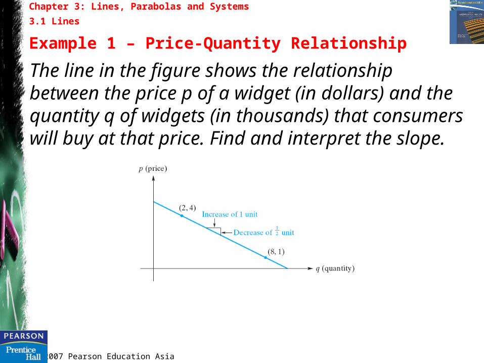
The line in the figure shows the relationship between the price p of a widget (in dollars) and the quantity q of widgets (in thousands) that consumers will buy at that price. Find and interpret the slope.
Chapter 3: Lines, Parabolas and Systems
3.1 Lines
Example 1 – Price-Quantity Relationship

2007 Pearson Education Asia
Solution:
The slope is
Chapter 3: Lines, Parabolas and Systems
3.1 Lines
Example 1 – Price-Quantity Relationship
2
1
28
41
12
12
ppm
Equation of line
• A point-slope form of an equation of the line through (x1, y1) with slope m is
1212
12
12
xxmyy
mxx
yy

2007 Pearson Education Asia
Find an equation of the line passing through (−3, 8) and (4, −2).
Solution:
The line has slope
Using a point-slope form with (−3, 8) gives
Chapter 3: Lines, Parabolas and Systems
3.1 Lines
Example 3 – Determining a Line from Two Points
7
10
34
82
m
026710
3010567
37
108
yx
xy
xy
2007 Pearson Education Asia
Chapter 3: Lines, Parabolas and Systems
3.1 Lines
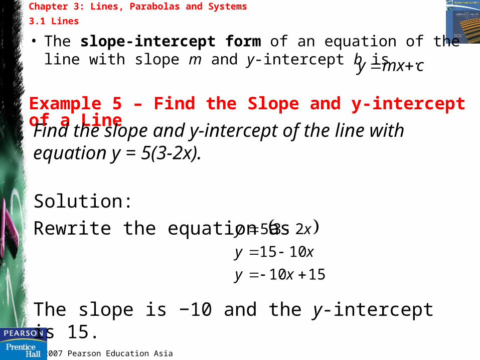
Example 5 – Find the Slope and y-intercept of a Line
• The slope-intercept form of an equation of the line with slope m and y-intercept b is . cmxy
Find the slope and y-intercept of the line with equation y = 5(3-2x).
Solution:
Rewrite the equation as
The slope is −10 and the y-intercept is 15.
1510
1015
235
xy
xy
xy

2007 Pearson Education Asia
a.Find a general linear form of the line whose slope-intercept form is
Solution:
By clearing the fractions, we have
Chapter 3: Lines, Parabolas and Systems
3.1 Lines
Example 7 – Converting Forms of Equations of Lines
43
2 xy
01232
043
2
yx
yx

2007 Pearson Education Asia
b. Find the slope-intercept form of the line having a general linear form
Solution:
We solve the given equation for y,
Chapter 3: Lines, Parabolas and Systems
3.1 Lines
Example 7 – Converting Forms of Equations of Lines
0243 yx
2
1
4
3
234
0243
xy
xy
yx

2007 Pearson Education Asia
Chapter 3: Lines, Parabolas and Systems
3.1 Lines
Parallel and Perpendicular Lines
• Parallel Lines are two lines that have the same slope.
• Perpendicular Lines are two lines with slopes m1 and m2 perpendicular to each other only if
21
1
mm

2007 Pearson Education Asia
Chapter 3: Lines, Parabolas and Systems
3.1 Lines
Example 9 – Parallel and Perpendicular Lines
The figure shows two lines passing through (3, −2). One is parallel to the line y = 3x + 1, and the other is perpendicular to it. Find the equations of these lines.

2007 Pearson Education Asia
Chapter 3: Lines, Parabolas and Systems
3.1 Lines
Example 9 – Parallel and Perpendicular Lines
Solution:
The line through (3, −2) that is parallel to y = 3x + 1 also has slope 3.
For the line perpendicular to y = 3x + 1,
113
932
332
xy
xy
xy
13
1
13
12
33
12
xy
xy
xy

2007 Pearson Education Asia
Chapter 3: Lines, Parabolas and Systems
3.2 Applications and Linear Functions3.2 Applications and Linear FunctionsExample 1 – Production Levels
Suppose that a manufacturer uses 100 lb of material to produce products A and B, which require 4 lb and 2 lb of material per unit, respectively.
Solution: If x and y denote the number of units produced of A and B, respectively,
Solving for y gives
0, where10024 yxyx
502 xy

2007 Pearson Education Asia
Chapter 3: Lines, Parabolas and Systems
3.2 Applications and Linear Functions
Demand and Supply Curves
• Demand and supply curves have the following trends:

2007 Pearson Education Asia
Chapter 3: Lines, Parabolas and Systems
3.2 Applications and Linear Functions
Example 3 – Graphing Linear Functions
Linear Functions
• A function f is a linear function which can be written as 0 where abaxxf
Graph and .
Solution:
12 xxf 3
215 ttg

2007 Pearson Education Asia
Chapter 3: Lines, Parabolas and Systems
3.2 Applications and Linear Functions
Example 5 – Determining a Linear Function
If y = f(x) is a linear function such that f(−2) = 6 and f(1) = −3, find f(x).
Solution: The slope is .
Using a point-slope form:
321
63
12
12
xx
yym
xxf
xy
xy
xxmyy
3
3
236 11

2007 Pearson Education Asia
Chapter 3: Lines, Parabolas and Systems
3.3 Quadratic Functions3.3 Quadratic Functions
Example 1 – Graphing a Quadratic Function
Graph the quadratic function .
Solution: The vertex is .
• Quadratic function is written aswhere a, b and c are constants and
22 bxaxxf0a
1242 xxxf
212
4
2
a
b
2 and 6
260
1240 2
x
xx
xx
The points are

2007 Pearson Education Asia
Chapter 3: Lines, Parabolas and Systems
3.3 Quadratic Functions
Example 3 – Graphing a Quadratic Function
Graph the quadratic function .Solution:
762 xxxg
312
6
2
a
b
23 x
2007 Pearson Education Asia
Chapter 3: Lines, Parabolas and Systems
3.3 Quadratic Functions
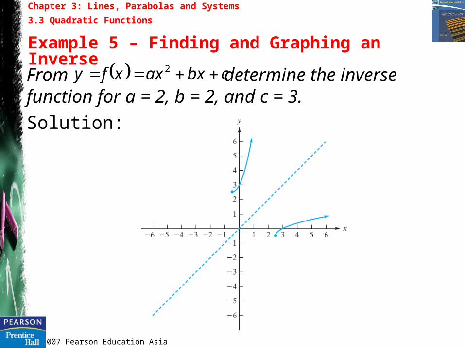
Example 5 – Finding and Graphing an Inverse
From determine the inverse function for a = 2, b = 2, and c = 3.
Solution:
cbxaxxfy 2

2007 Pearson Education Asia
Chapter 3: Lines, Parabolas and Systems
3.4 Systems of Linear Equations3.4 Systems of Linear Equations
Two-Variable Systems
• There are three different linear systems:
• Two methods to solve simultaneous equations:
a) elimination by addition
b) elimination by substitution
Linear system(one solution)
Linear system(no solution)
Linear system(many solutions)
2007 Pearson Education Asia
Chapter 3: Lines, Parabolas and Systems
3.4 Systems of Linear Equations
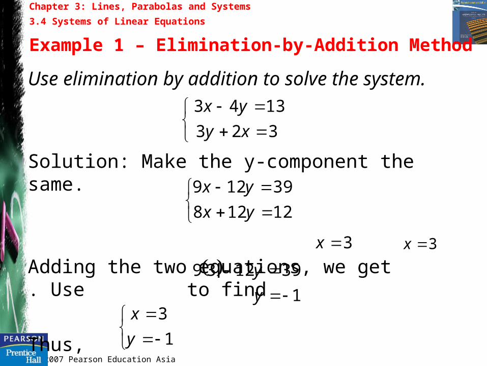
Example 1 – Elimination-by-Addition Method
Use elimination by addition to solve the system.
Solution: Make the y-component the same.
Adding the two equations, we get . Use to find
Thus,
323
1343
xy
yx
12128
39129
yx
yx
3x
1
391239
y
y
1
3
y
x
3x

2007 Pearson Education Asia
Chapter 3: Lines, Parabolas and Systems
3.4 Systems of Linear Equations
Example 3 – A Linear System with Infinitely Many Solutions
Solve
Solution: Make the x-component the same.
Adding the two equations, we get .
The complete solution is
12
5
2
125
yx
yx
25
25
yx
yx
00
ry
rx
52

2007 Pearson Education Asia
Chapter 3: Lines, Parabolas and Systems
3.4 Systems of Linear Equations
Example 5 – Solving a Three-Variable Linear System
Solve
Solution: By substitution, we get
Since y = -5 + z, we can find z = 3 and y = -2. Thus,
63
122
32
zyx
zyx
zyx
63
5
1573
zyx
zy
zy
1
2
3
x
y
z

2007 Pearson Education Asia
Chapter 3: Lines, Parabolas and Systems
3.4 Systems of Linear Equations
Example 7 – Two-Parameter Family of Solutions
Solve the system
Solution:
Multiply the 2nd equation by 1/2 and add to the 1st equation,
Setting y = r and z = s, the solutions are
8242
42
zyx
zyx
00
42 zyx
sz
ry
srx
24

2007 Pearson Education Asia
Chapter 3: Lines, Parabolas and Systems
3.5 Nonlinear Systems3.5 Nonlinear Systems
Example 1 – Solving a Nonlinear System
• A system of equations with at least one nonlinear equation is called a nonlinear system.
Solve (1)
(2)
Solution: Substitute Eq (2) into (1),
013
0722
yx
yxx
7 or 8
2 or 3
023
06
071322
2
yy
xx
xx
xx
xxx

2007 Pearson Education Asia
Chapter 3: Lines, Parabolas and Systems
3.6 Applications of Systems of Equations3.6 Applications of Systems of Equations
Equilibrium
• The point of equilibrium is where demand and supply curves intersect.

2007 Pearson Education Asia
Chapter 3: Lines, Parabolas and Systems
3.6 Applications of Systems of Equations
Example 1 – Tax Effect on Equilibrium
Let be the supply equation for a manufacturer’s product, and suppose the demand equation is .
a. If a tax of $1.50 per unit is to be imposed on the manufacturer, how will the original equilibrium price be affected if the demand remains the same?
b. Determine the total revenue obtained by the manufacturer at the equilibrium point both before and after the tax.
50100
8 qp
65100
7 qp

2007 Pearson Education Asia
Chapter 3: Lines, Parabolas and Systems
3.6 Applications of Systems of Equations
Example 1 – Tax Effect on Equilibrium
Solution:
a. By substitution,
and
After new tax,
and
100
50100
865
100
7
q
qq 5850100100
8p
70.5850.51100100
8p
90
65100
750.51100
100
8
q
q
2007 Pearson Education Asia
Chapter 3: Lines, Parabolas and Systems
3.6 Applications of Systems of Equations
Example 1 – Tax Effect on Equilibrium
Solution:
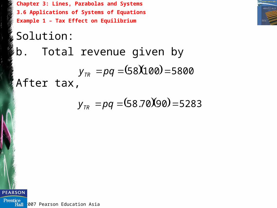
b. Total revenue given by
After tax, 580010058 pqyTR
52839070.58 pqyTR

2007 Pearson Education Asia
Chapter 3: Lines, Parabolas and Systems
3.6 Applications of Systems of Equations
Break-Even Points
• Profit (or loss) = total revenue(TR) – total cost(TC)
• Total cost = variable cost + fixed cost
• The break-even point is where TR = TC.
FCVCTC yyy

2007 Pearson Education Asia
Chapter 3: Lines, Parabolas and Systems
3.6 Applications of Systems of Equations
Example 3 – Break-Even Point, Profit, and Loss
A manufacturer sells a product at $8 per unit, selling all that is produced. Fixed cost is $5000 and variable cost per unit is 22/9 (dollars).
a. Find the total output and revenue at the break-even
point.
b. Find the profit when 1800 units are produced.
c. Find the loss when 450 units are produced.
d. Find the output required to obtain a profit of $10,000.

2007 Pearson Education Asia
Chapter 3: Lines, Parabolas and Systems
3.6 Applications of Systems of Equations
Example 3 – Break-Even Point, Profit, and Loss
Solution:
a. We have
At break-even point,
and
b.
The profit is $5000.
50009
22
8
qyyy
qy
FCVCTC
TR
900
50009
228
q
yy TCTR
72009008 TRy
5000500018009
2218008
TCTR yy
Top Related