


Languages
Pages
Legal


1
Estimation of Finite Estimation of Finite Population Mean Using Population Mean Using
Ranked Set Ranked Set Two-stage Sampling Two-stage Sampling
DesignDesign
ByBy
U C Sud and Dwidesh U C Sud and Dwidesh MishraMishra
IASRI, New Delhi-110012IASRI, New Delhi-110012

2
• The method of Ranked Set Sampling (RSS) was first The method of Ranked Set Sampling (RSS) was first introduced by McIntyre (1952) as a cost-efficient introduced by McIntyre (1952) as a cost-efficient alternative to simple random sampling for situations alternative to simple random sampling for situations where outside information is available allowing one to where outside information is available allowing one to rank small sets of sampling units according to the rank small sets of sampling units according to the character of interest without actually quantifying the character of interest without actually quantifying the
units.units. • McIyntyre was concerned with estimating agricultural McIyntyre was concerned with estimating agricultural
yields where the ranking could be done on the basis of yields where the ranking could be done on the basis of visual inspection.visual inspection.
• One of the strengths of the method, however, is that One of the strengths of the method, however, is that its implementation and performance require only that its implementation and performance require only that ranking be possible but they do not depend in any way ranking be possible but they do not depend in any way on how the ranking is accomplishedon how the ranking is accomplished
IntroductionIntroduction

3
The Method of RSSThe Method of RSS
• A A basic cyclebasic cycle of the method involves the random selection of of the method involves the random selection of mm22 units from the population. These units are randomly units from the population. These units are randomly partitioned into partitioned into mm subsets, each containing subsets, each containing mm sampling sampling units. The members of every subset are ranked according to units. The members of every subset are ranked according to the character of interest.the character of interest.
• Then the lowest ranked member is quantified from the first Then the lowest ranked member is quantified from the first set, the second lowest ranked member is quantified from set, the second lowest ranked member is quantified from the second set, and so on until the highest ranked member the second set, and so on until the highest ranked member of the last set is quantified.of the last set is quantified.
• This yields m quantification from among the mThis yields m quantification from among the m22 selected selected units. Since m is usually taken as small in order to facilitate units. Since m is usually taken as small in order to facilitate the ranking, there may not be enough measurements for the ranking, there may not be enough measurements for reasonable inference and the basic cycle is repeated r times reasonable inference and the basic cycle is repeated r times to give n=mr quantifications out of r selected units.to give n=mr quantifications out of r selected units.

4
• Let us take a set-size m=3 with r=4Let us take a set-size m=3 with r=4• Then the sampling scheme can be shown by the following diagramThen the sampling scheme can be shown by the following diagram• Here each row indicates a judgement ordered sample for each cycle. Encircled Here each row indicates a judgement ordered sample for each cycle. Encircled
units are quantified. Out of 36 units drawn, 12 units have been quantifiedunits are quantified. Out of 36 units drawn, 12 units have been quantified
Cycle Cycle RankRank
11 22 33
11 -- --
-- --
-- --
22 -- --
-- --
-- --
33 -- --
-- --
-- --
44 -- --
-- --
-- --

5
Contd.Contd.• Let XLet X1111, X, X1212,…, X,…, X1m1m, X, X2222,…,X,…,X2m2m,…,X,…,Xm1m1,…,X,…,Xmmmm be independent random be independent random
variables all having the same cumulative distribution function variables all having the same cumulative distribution function F(x). Also let F(x). Also let
• XXi(1)i(1), X, Xi(2)i(2),…, X,…, Xi(m) i(m) denote the corresponding order statistics ofdenote the corresponding order statistics of , X, Xi1i1,,…,X…,Xi2i2,…,X,…,Xiiii,…,X,…,Ximim
• (i=1,2,…,m). Then X(i=1,2,…,m). Then X1(1)1(1), X, X2(2)2(2),…, X,…, Xm(m) m(m) is the ranked set sampleis the ranked set sample
(considering one cycle only), since X(considering one cycle only), since X i(i)i(i)is the i-th order statistic in is the i-th order statistic in the i-th sample.the i-th sample.
• The value XThe value Xijij for the randomly drawn units can be arranged as in for the randomly drawn units can be arranged as in the following diagram:the following diagram:
• SetSet
mmmm
m
XXXm
XXX
XXX
21
232221
11211
....
2
1

6
Contd.Contd.• After ranking the units appear as:After ranking the units appear as:
)(
)2(2
)1(1
**
....
**2
**1
mmXm
X
X
)()2()1(
3(2)2(2)1(2
)(1)2(1)1(1
....
)2
1
mmmm
m
XXXm
XXX
XXX
The quantified units appear as
m:iX
7
ExamplesExamples• RSS is very useful in environmental and ecological sampling RSS is very useful in environmental and ecological sampling
where exact measurement (or quantification) of a selected unit is where exact measurement (or quantification) of a selected unit is either difficult or expensive in terms of time, money or labor, but either difficult or expensive in terms of time, money or labor, but where ranking of a small set of selected units according to the where ranking of a small set of selected units according to the characteristic of interest can be done with reasonable success on characteristic of interest can be done with reasonable success on the basis of visual inspection or other rough method not requiring the basis of visual inspection or other rough method not requiring actual measurement.actual measurement.
• Thus if the interest lies in estimating the mean height of the Thus if the interest lies in estimating the mean height of the sampled trees, then measurement of the height of the trees could sampled trees, then measurement of the height of the trees could pose a problem, but it would be relatively easy to rank small sets pose a problem, but it would be relatively easy to rank small sets of trees on the basis of visual inspection.of trees on the basis of visual inspection.
• In situations where visual inspection is not directly available In situations where visual inspection is not directly available ranking can be done on the basis of a covariate that is more ranking can be done on the basis of a covariate that is more accessible and also correlated with the character of interest.accessible and also correlated with the character of interest.
• Thus for estimating volume of trees one can carry out ranking on Thus for estimating volume of trees one can carry out ranking on the basis of diameter of the trees.the basis of diameter of the trees.

8
• Performance of the RSS estimator is generally benchmarked Performance of the RSS estimator is generally benchmarked
against that of simple random sampling (SRS) estimator against that of simple random sampling (SRS) estimator with the same number of quantifications. For this purpose, one with the same number of quantifications. For this purpose, one may employ either the may employ either the relative precision,relative precision,
•
• Or the relative savings, Or the relative savings,
• There was little follow up on McIntyre’s (1952) proposal until There was little follow up on McIntyre’s (1952) proposal until late 1960s when Hall and Dell (1966) published a field late 1960s when Hall and Dell (1966) published a field evaluation and Takahasi and Wakimoto (1968) developed the evaluation and Takahasi and Wakimoto (1968) developed the statistical theory for the RSS method. When sampling is from a statistical theory for the RSS method. When sampling is from a continuous population and the ranking is perfect, Takahasi and continuous population and the ranking is perfect, Takahasi and Wakimoto proved that is unbiased for and Wakimoto proved that is unbiased for and is at least as efficient as . is at least as efficient as .
RSS
SRSRPˆvar
ˆvar
RPRS 11
RSS
SRS
SRS
Theory of RSS

9
• They also obtained the variance of the RSS estimator asThey also obtained the variance of the RSS estimator as
• where is the population variance and is the expected i-th out where is the population variance and is the expected i-th out of m order statistic from the population. They also established the boundof m order statistic from the population. They also established the bound
• or or
• The upper bound indicates that ranked set sampling can result in very The upper bound indicates that ranked set sampling can result in very substantial savings when compared with simple random sampling. substantial savings when compared with simple random sampling. Specifically, the method can result in savings in the number of Specifically, the method can result in savings in the number of quantifications by as much as 33, 50, 60, 67 percent when m=2, 3, 4, 5 quantifications by as much as 33, 50, 60, 67 percent when m=2, 3, 4, 5 respectively.respectively.
2
m
imiRSS mmr
2:
2 11ˆvar
mi:
2
11
m
RP
Contd.
1m
1mRS1

10
ReviewReview• Stokes (1979) considered the use of concominant variable at the Stokes (1979) considered the use of concominant variable at the
estimation stage in the context of RSSestimation stage in the context of RSS
• Stokes (1980) dealt with the problem of estimation of population Stokes (1980) dealt with the problem of estimation of population variancevariance
• Dell and Clutter (1972) considered the problem of ranking errorsDell and Clutter (1972) considered the problem of ranking errors
• Philip and Lam (1997) developed a regression estimator for RSSPhilip and Lam (1997) developed a regression estimator for RSS
11
RSS in the Context of Finite RSS in the Context of Finite Population SamplingPopulation Sampling
• Early developments in RSS were concerned with sampling from infinite population.
• Patil et al. (1994) were the first to consider the situation of sampling from finite population.
• Explicit expressions were obtained for the variance of the RSS estimator and for its precision relative to that of simple random sampling without replacement.
• Krishna (2002) extended the theory of RSS to the case of sampling from a finite population by utilising a Horvitz-Thomson estimator for the estimation of the finite population mean.
• Calculation of • Calculation of is tedious
, iji
ij

12
Three different cases have been studied. In the first case the SRS is used at the 1st stage of sampling and RSS at the 2nd stage of sampling. Similarly, the RSS is used at 1st stage and SRS at the 2nd stage in second case. In the third case the RSS is used in both the stages of sampling. In each of the cases efficiency comparisons of RSS based estimators have been made with SRS based estimators with the help of real data when the sampling is SRS at both the stages of sampling.
Let there be a finite population of N primary stage units, a-th primary stage unit is of size M. Let be the value of unit pertaining to b-th secondary stage unit (ssu) of a-th primary stage unit (psu).
However, the contributions made by Patil et al. (1994) and Krishna (2002) were limited to the case of uni-stage sampling designs.
RSS for Two – stage sampling designs
RSS for Two - Stage Sampling Design
abx

13
M
baba x
MX
1
1
= mean per ssu in the a-th psu
N
a
M
babxNM
X1 1
1
= Population mean
Case 1: SRS at first stage and RSS at second stage
Let a sample of size ‘n’ be drawn from ‘N’ by SRSWOR. Also, let a set of size m be selected at random and without replacement from M using RSS.
Without any loss of generality we assume that
N1,2,...,a )...( 21 aMaa xxx
Contd.

14
Case 1: SRS at first stage and RSS at Case 1: SRS at first stage and RSS at second stagesecond stage
• Define the eventDefine the event
}{ sk
such that the k-th ranked unit in the subset is the s-th ranked unit in the population of ssu.
Also write,
}Pr{ skAsak
akA M- sakAand let denote the - dimensional column vector having
as its s-th component
'

15
Contd.Contd.
Mak
sak
2ak
1ak
'ak A . . . A . . . A AA
It may be noted that sakA is given by
,1
1
m
Mkm
sM
k
s
Ms ,...,2,1
):( mkaxIf
is the quantification of the k-th ranked unit from the set, then

16
Contd.Contd.
):():( ][ mkamka XxE
M
sasmkaas xxx
1):( ]Pr[
M
sas skx
1})Pr({
M
s
sakasAx
1
aak xA 2
):():( ][ mkaxmkaxV
22 )( aakaak xAxA

17
Contd.Contd.
2ax is the component wise square of ax
Next, we study the joint distribution of the order statistics from two disjoint sets. Let two disjoint sets each of size m
be drawn without replacement from MWrite },{ tjsk
for the event that the k-th ranked unit from set 1 has rank s and the j-th ranked unit from set 2 has rank t in the population of size .M
We define
},Pr{ tjskBstakj

18
Following Patil et al. (1994), it may be seen that
kmst
akj
mm
Mjm
kmtM
j
kt
km
tMst
k
s
B0
,
1
1
1
1
1
Let akjB be the MM matrix with stakjB as its (s,t)th component.
Notice that ajkakj BB , since tsajk
stakj BB .Let 1):( mkax and .
2):( mjax be the quantification of the k-th and j-th ranked units from set 1 and set 2, respectively. Then ,
Contd.

19
Contd.Contd.
2):(1):( , mjamka xx is given by
],[ 2):(1):( mjamka xxCov akjC aajakakja xAABx )(
The covariance between

20
Contd.Contd.
Let mr sets, each of size m, be selected randomly using RSS and without replacement from the a-th psu. Let the lowest ranked unit be quantified in each of the first ‘r’ sets-
rmamama XXX ):1(2):1(1):1( ,...,,
In each of the next r sets, the second ranked unit is quantified to give:
rmamama XXX ):2(2):2(1):2( ,...,,
This process continues until the highest ranked unit is quantified in each of the last r sets:
21
Contd.Contd.
rmmammamma XXX ):(2):(1):( ,...,,
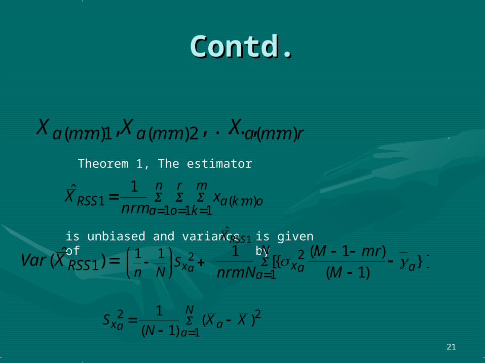
Theorem 1, The estimator
n
a
r
o
m
komkaRSS x
nrmX
1 1 1):(1
1ˆ
is unbiased and variance of 1ˆRSSX is given by
)ˆ( 1RSSXVar
211
axSNn}]
)1(
)1({[
1 2
1aax
N
a M
mrM
nrmN
N
aaax XX
NS
1
22 )()1(
1

22
Proof of the resultsProof of the results
a amMMM
mm )12)...(1(
)!1(!
)()( aaaaa xx
The matrix is symmetric with zeroes on the diagonal, it is calculated by
*
1,
m
kakkB
mm
M
Proof:To prove that the estimator 1RSSX is unbiased, we proceed as
follows:
A program has been made in the language Turbo ‘C’ to calculate TA program has been made in the language Turbo ‘C’ to calculate T

23
Contd.Contd.
]1
[)ˆ(1 1 1
):(21121
n
a
r
o
m
komkaRSS x
nrmEEXEE
]1
[1
1 1 1):(21
n
a
r
o
m
komkaxrm
En
E
][11
1 1 1):(21
n
a
r
o
m
komkaxE
rmnE
n
1a
r
1o
m
1kaak1 xA
rm
1
n
1E
n
a
r
o
m
k
M
sas
sak xA
rmnE
1 1 1 11
11
asn
a
M
s
m
k
sak xA
mnE )(
11
1 1 11

24
Contd.Contd.
n
a
M
sasxMn
E1 1
111
n
aaXn
E1
11
N
aaXN 1
1
)ˆ()ˆ()ˆ( 1211211 RSSRSSRSS XEVXVEXV
)ˆ( 12 RSSXV [arV ]xnrm
1 n
1a
r
1o
m
1ko)m:k(a
m
1k
m
1k
m
1j
m
kakkakj
22)m:k(a
n
1a 222}]CCrr{
mr
1[
n
1
}])()1(
)1({
1[
1
11
2):(
2
1 22
m
kakk
m
kamkaax
n
aCXX
M
mrMm
rmn
)X(V 1RSS2}])()(
1
)1(
)1({
1[
1
1
2
12
m
kaaakkaaax
n
aXxBXx
mM
mrM
rmn
After centering

25
Contd.
}])1(
)1({
1[
1 2
12 aaxn
a M
mrM
rmn
)X(VE 1RSS21 }])1M(
)mr1M({
rm
1[
nN
1a
2ax
N
1a
]}xrm
1{E
n
1[V)X(EV
r
1o
m
1ko)m:k(a
n
1a211RSS21
2
axSN
1
n
1

26
Assume that a sample of size ‘m’ is selected by SRSWOR from the a-th psu a=1,2,…,N. Further, we assume that a set of size ‘n’ is selected from ‘N’ by RSS. Also, as in Case 1, we assume that the psu’s are increasingly arranged. Define the event
such that the a-th ranked unit in the subset is the s-th ranked unit in the population of psu’s.
Define }Pr{ saAsa
Nasaaaa AAAAA . . . . . . 21' be the 1N row vector having
Case2: RSS at first stage and Case2: RSS at first stage and SRS at second stageSRS at second stage

27
Contd.Contd.
as its s-th component
n
Nan
sN
a
s
Asa1
1
m
bbnana x
mx
1):():(
1= sample mean for the a-th psu.
M
bbnabna x
MxE
1):():(2
1][
):( nasXXAa
'2
):():(1 )( naxnaXV 2'2' )( XAXA aa
naXE :1
saA
s=1,2,…,N; a=1,2,…,n

28
Contd.Contd.
To study the joint distribution of the order statistics from disjoint sets each of size ‘n’ drawn by without replacement using RSS, let
},{ tcsa be the event that the a-th ranked unit from set 1 has rank s in the population and the c-th ranked unit from set 2 has rank t in the population.
},Pr{ tcsaBstac
anst
ac
nn
Ncm
amtM
c
at
am
tMst
a
s
B0
,
1
1
1
1
1

29
Contd.Contd.
Let 1):( nax and 2):( ncxbe the quantification of the a-th and c-th ranked units from set 1 and set 2, respectively. Then ,
2):( ncx ] xBx ac
acncna CxxCov ],[ ):():( xAABx caac )(
Moments of the estimator of population mean:Let nr sets each of size n be selected randomly and without replacement from a population of N psu’s. Let the lowest ranked unit be quantified in each of the first r sets
rnnn XXX ):1(,2):1(1):1( ...,,
1:[ naxE

30
Contd.Contd.
Similarly, in each of the next r sets, the second ranked unit is quantified to give
rnnn XXX ):2(,2):2(1):2( ...,,
This process continues until the highest raked unit is quantified in each of the last r sets:
rnmnmnm XXX ):(,2):(1):( ...,,
Thus, the proposed estimator of population mean, when the sample at the first stage is selected by RSS and at the second stage by SRS, is given by
n
a
r
o
m
bbonaRSS x
nrmX
1 1 1),):((2
1ˆ
31
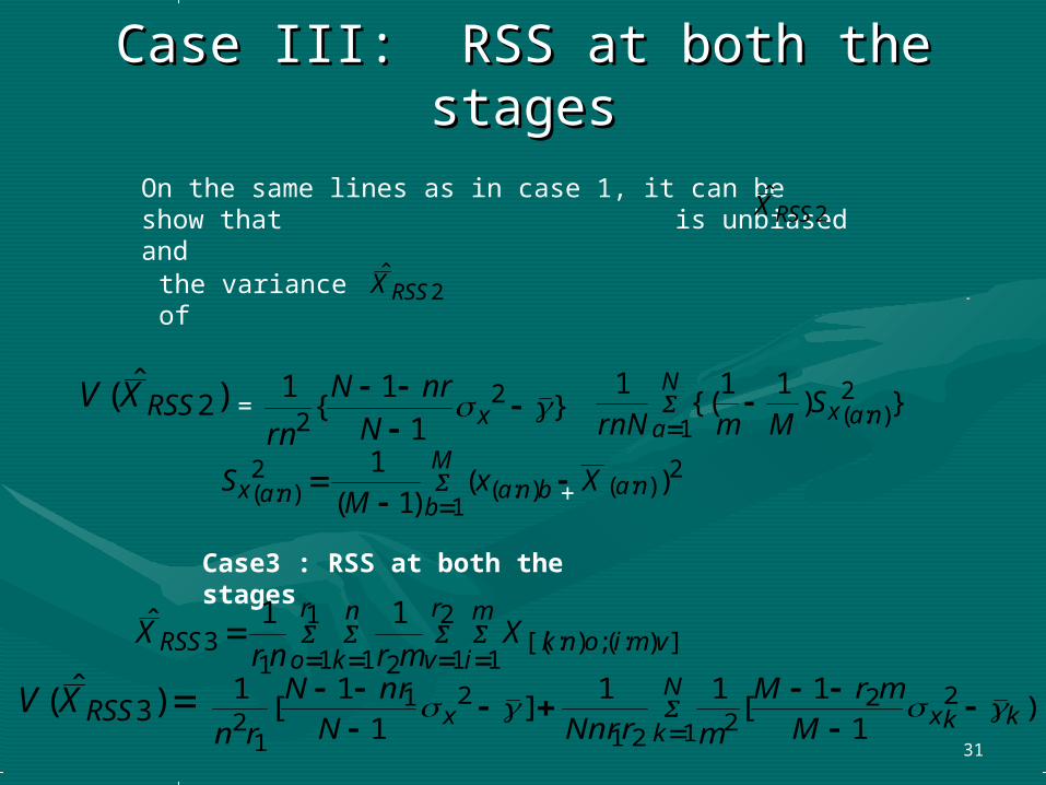
Case III: RSS at both the stagesCase III: RSS at both the stages
On the same lines as in case 1, it can be show that is unbiased and 2
ˆRSSX
the variance of 2ˆRSSX
)ˆ( 2RSSXV = }1
1{
1 22
xN
nrN
rn
+
N
anaxSMmrnN 1
2):( })
11{(
1
2
1):():(
2):( )(
)1(
1
M
bnabnanax Xx
MS
Case3 : RSS at both the stages
2
1 1]):(;):[(
1
1 1 213
11ˆ r
v
m
ivmionk
r
o
n
kRSS X
mrnrX
)ˆ( 3RSSXV )]1
1[
11]
1
1[
1 22
1 221
21
12 kkx
N
kx M
mrM
mrNnrN
nrN
rn

32
For the purpose of comparing the RSS and the SRS based estimator an empirical study was carried out where in a part of the data of wheat crop for an experimental station as given in Singh et al. (1979) was taken. The data comprised 9 fields each field having 4 plots. (Set I). (The population values of were 4.163 and 0.306 respectively).2 and
For RSS protocol, plots in each field were ranked according to the perceived weight of wheat yield. Using this data, estimators of population mean based on RSS and SRS were considered for the three cases dealt with earlier.
3. Empirical Study3. Empirical Study

33
2 and
were 38.05 and 11.23 respectively). The data comprised 9 blocks and 4 societies in each of the block.Finally data on number of persons in a household given in Raj (1971) was also utilized to compare the performance of RSS and SRS based estimators. (Set III). (The population values of 2 and
were 7052 and 0.093 respectively). Here also the data comprised 9 households and 4 persons in a household
Another data set given in Singh and Mangat (1996) on outstanding loans of farmers affiliated to cooperatives was utilized to compare the performance of RSS and SRS based estimators. (Set II). The population values of

34
Table 2.1 Per cent gain in precision of RSS based estimators over SRS based estimators
CaseCase StageStage DesignDesign EstimatorEstimator S.E.S.E.of the estimatorof the estimator
Per cent gain in Per cent gain in precision precision
Set ISet I
11 11 SRSSRS 5.395.39 10.2110.21
22 RSSRSS
22 11 RSSRSS 5.605.60 1.851.85
22 SRSSRS
33 11 RSSRSS 5.335.33 12.4612.46
22 RSSRSS
44 11 SRSSRS 5.94 5.94 --------------
22 SRSSRS
1ˆRSSX
2ˆRSSX
3ˆRSSX
SRSX

35
Set IISet II
11 11 SRSSRS 1.031.03 10.6710.67
22 RSSRSS
22 11 RSSRSS 1.111.11 2.702.70
22 SRSSRS
33 11 RSSRSS 1.011.01 12.8712.87
22 RSSRSS
44 11 SRSSRS 1.141.14 --------------
22 SRSSRS
SRSX
3ˆRSSX
2ˆRSSX
1ˆRSSX

36
Set IIISet III
11 11 SRSSRS 0.1990.199 15.5715.57
22 RSSRSS
22 11 RSSRSS 0.2050.205 12.1912.19
22 SRSSRS
33 11 RSSRSS 0.1940.194 18.5518.55
22 RSSRSS
44 11 SRSSRS 0.2300.230 --------------
22 SRSSRS
SRSX
2ˆRSSX
3ˆRSSX
1ˆRSSX

37
References:References:•Dell, T.R. and Clutter, J.L.(1972). Ranked set sampling theory with order statistics background. Biometrics, 28, 545-553.
•Halls, L.K. and Dell, T.R. (1966). Trail of ranker set sampling for forage yields. Forest Science, 12, 22-26.
•Krishna, Pravin (2002). Some aspects of ranked set sampling from finite population. M.Sc.Thesis of I.A.R.I., New Delhi-12.
•McIntyre, G A (1952). A method of unbiased selective sampling using ranked sets. Australian Journal of Agricultural Research, 3, 385-390.
•Patil, G.P., Sinha, A. K. and Taillie, C. (1993). Ranked set sampling from a finite population in the presence of a trend on a site. Journal of Applied Statistical Science. Vol.1, No. 1, 51-65.
•Patil, G.P., Sinha, A. K. and Taillie, C. (1994). Ranked set sampling. Handbook of Statistics. 12, (eds. Patil, G. P. and Rao, C. R.), 167-198, North-Holland, Amsterdam.
•Patil, G.P., Sinha, A. K. and Taillie, C. (1995). Finite population corrections for ranked set sampling. Annals of Institute of Statistical Mathematics. Vol.47, No. 4, 621-636.

38
• Raj, D. (1971). The Design of Sample Surveys. Mcgraw-Hill Book Co., New
York.
• Singh, D., Singh, P. and Kumar, P. (1979). Hand Book on Sampling
Methods. Indian Agricultural Statistics Research Institute, New Delhi.
• Singh, R and Mangat, N.P.S. (1996). Elements of Survey Sampling. Kluwer
Academic Publisher, pp 388.
• Stokes, S L (1977). Ranked set sampling with concominant variables.
Communication in statistics, Theory and Methods, 6, 1207-1211.
• Stokes, S L (1980). Estimation of variance using judgement order ranked
set samples. Biometrics, 36, 35-42.

39
• Takahasi, K. and Wakimoto, K. (1968). On biased estimates of the
population mean based on the sample stratified by means of ordering.
Annals of the Institute of Statistical Mathematics, 20, 1-31.
• Yu, Philip L.H. and Lam K. (1997). Regression estimator in ranked set
sampling, Biometrics, 53, 1070-1080.

40
THANKS
Top Related