


Languages
Pages
Legal


A General Multitiered Supply Chain Network Model of Quality Competition with Suppliers
Dong Li1 and Anna Nagurney2
1Department of Management & Marketing
College of Business
Arkansas State University, State University, Arkansas 72467
2Department of Operations and Information Management
Isenberg School of Management
University of Massachusetts, Amherst, Massachusetts 01003
revised July and September 2015
International Journal of Production Economics (2015), 170, pp 336-356.
Abstract
In this paper, we develop a general multitiered supply chain network equilibrium model consisting
of competing suppliers and competing firms who purchase components for the assembly of their final
branded products and, if capacity permits, and it enhances profits, produce their own components.
The competitive behavior of each tier of decision-makers is described along with their strategic vari-
ables, which include quality of the components and, in the case of the firms, the quality of the assembly
process itself. The governing equilibrium conditions of the supply chain network are formulated as
a variational inequality and qualitative properties are presented. The algorithm, accompanied with
convergence results, is then applied to numerical supply chain network examples, along with sensi-
tivity analysis in which the impacts of capacity disruptions and complete supplier elimination are
investigated.
Keywords: supply chains, networks, suppliers, quality competition, game theory, variational inequal-
ities
1

1. Introduction
Quality has been recognized as “the single most important force leading to the economic growth of
companies in international markets” (Feigenbaum (1982) page 22), and, in the long run, as the most
important factor affecting a business unit’s performance and competitiveness, relative to the quality
levels of its competitors (Buzzell and Gale (1987)). Many firms, however, with pressure to lower their
costs, continue to subcontract manufacturing to lower cost countries globally, with their supply chain
networks being more exposed to quality failures (Marucheck et al. (2011)) and with the policing and
monitoring of product safety also extremely difficult (Tang (2008)).
In recent years, there have been numerous examples of finished product failures due to the poor
quality of a suppliers’ components. For example, the toy manufacturer, Mattel, in 2007, recalled
19 million toy cars because of suppliers’ lead paint and poorly designed magnets, which could harm
children if ingested (Story and Barboza (2007)). In 2013, four Japanese car-makers, along with BMW,
recalled 3.6 million vehicles because the airbags supplied by Takata Corp., the world’s second-largest
supplier of airbags, were at risk of rupturing and injuring passengers (Kubota and Klayman (2013)).
The recalls are still ongoing and have expanded to other companies as well (Tabuchi and Jensen
(2014)). Most recently, the defective ignition switches in General Motors (GM) vehicles, which were
produced by Delphi Automotive in Mexico, have been linked to 13 deaths, due to the fact that the
switches could suddenly shut off engines with no warning (Stout, Ivory, and Wald (2014) and Bomey
(2014)). In addition, serious quality shortcomings and failures associated with suppliers have also
occurred in finished products such as aircraft (Drew (2014)), pharmaceuticals (Rao (2014)), and also
food (Strom (2013) and McDonald (2014)). In 2009, over 400 peanut butter products were recalled
after 8 people died and more than 500 people, half of them children, were sickened by salmonella
poisoning, the source of which was a peanut butter plant in Georgia (Harris (2009)).
Product quality is an important feature that enables firms to maintain and even to improve their
competitive advantage and reputation. However, numerous finished products are made of raw materials
as well as components and it is usually the case that the components and materials are produced and
supplied not by the firms that process them into products but by suppliers in globalized supply chain
networks. For example, Sara Lee bread, an everyday item, is made with flour from the US, vitamin
supplements from China, gluten from Australia, honey from Vietnam and India, and other ingredients
from Switzerland, South America, and Russia (Bailey (2007)), let alone automobiles and aircrafts
which are made up of thousands of different components.
Therefore, the quality of a finished/final product depends not only on the quality of the firm that
produces and delivers it, but also on the quality of the components provided by the firm’s suppliers
(Robinson and Malhotra (2005) and Foster (2008)). It is the suppliers that determine the quality of
the materials that they purchase as well as the standards of their manufacturing activities. However,
suppliers may have less reason to be concerned with quality (Nagurney, Li, and Nagurney (2013)
and Amaral, Billington, and Tsay (2006)). In Mattel’s case, some of the suppliers were careless,
others flouted rules, and others simply avoided obeying the rules (Tang (2008)). With non-conforming
2

components, it may be challenging and very difficult for firms to produce high quality finished products
even if they utilize the most superior production and transportation delivery techniques.
Furthermore, since suppliers may be located both on-shore and off-shore, supply chain networks
of firms may be more vulnerable to disruptions around the globe than ever before. Photos of Honda
automobiles under 15 feet of water were some of the most appalling images of the impacts of the
Thailand floods of 2011. Asian manufacturing plants affected by the catastrophe were unable to
supply components for cars, electronics, and many other products (Kageyama (2011)). In the same
year, the triple disaster in Fukushima affected far more than the manufacturing industry in Japan. A
General Motors plant in Louisiana had to shut down due to a shortage of Japanese-made components
after the disaster took place (Lohr (2011)). Under such disruptions, suppliers may not even be capable
of performing their production tasks, let alone guaranteeing the quality of the components.
In addition, the number of suppliers that a firm may be dealing with can be vast. For example,
according to Seetharaman (2013), Ford, the second largest US car manufacturer, had 1,260 suppliers
at the end of 2012 with Ford purchasing approximately 80 percent of its parts from its largest 100
suppliers. Due to increased demand, many of the suppliers, according to the article were running “flat
out” with the consequence that there were quality issues. In the case of Boeing, according to Denning
(2013), complex products such as aircraft involve a necessary degree of outsourcing, since the firm
lacks the necessary expertise in some areas, such as, for example, engines and avionics. Nevertheless,
as noted therein, Boeing significantly increased the amount of outsourcing for the 787 Dreamliner
airplane over earlier planes to about 70 percent, whereas for the 737 and 747 airplanes it had been
at around 35-50 percent. Problems with lithium-ion batteries produced in Japan grounded several
flights and resulted in widespread media coverage and concern for safety of the planes because of that
specific component (see Parker (2014)).
Recently, there has been increasing attention from researchers to supplier-manufacturer supply
chain networks with quality in both operations research and economics. However, in the literature,
most models are based on a single firm - single supplier supply chain network (cf. Reyniers and
Tapiero (1995), Tagaras and Lee (1996), Starbird (1997), Baiman, Fischer, and Rajan (2000), Lim
(2001), Hwang, Radhakrishnan, and Su (2006), Zhu, Zhang, and Tsung (2007), Chao, Iravani, and
Savaskan (2009), Hsieh and Liu (2010), and Xie et al. (2011)), which, given the reality of many
finished product supply chains, as noted above, may be limiting in terms of both scope and practice.
Specifically, although focused, simpler models, may yield closed form analytical solutions, more general
frameworks, that are computationally tractable, are also needed, given the size and complexity of real-
world global supply chains.
In addition to the above mentioned literature, the following papers considered more than one firm
and/or supplier in their models. Economides (1999) studied a dual-monopolist problem with two
components, and concluded that vertical integration could guarantee higher quality. El Ouardighi and
Kim (2010) formulated a dynamic game in which a supplier collaborated with two firms on design
quality improvements. Pennerstorfer and Weiss (2012) studied a wine supply chain network with
3

multiple suppliers and firms, and each firm made identical decisions on quality. Furthermore, in the
models developed by Hong and Hayya (1992), Rosenthal, Zydiak, and Chaudhry (1995), Jayaraman,
Srivastava, and Benton (1999), Ghodsypour and O’Brien (2001), and Rezaei and Davoodi (2008),
multiple firms and/or suppliers were involved with quality being considered as input parameters, and
the decisions on quality were not provided.
Different from the above models, the main contributions of this paper are: 1. We formulate
the supply chain network problem with multiple nonidentical competing firms and their potential
suppliers who also compete in quality. 2. The model is general and not limited to a small number of
firms, suppliers, or components or limited to specific functional forms in terms of costs or demand price
functions. 3. The solution of the proposed game theory model provides equilibrium decisions on the in-
house and contracted component production and quality levels, component prices, product quantities,
and the quality preservation/decay levels of the assembly processes simultaneously. Decisions on the
prices and quality levels of the final products are determined through information provided via the
demand price functions and the quality aggregation functions. 4. Based on this model, the value of
each supplier to each firm can be identified, as illustrated in the analysis in Section 5. This information
is crucial in facilitating strategy design and development in supplier management especially in response
to supplier disruptions. 5. Along with the general multitiered supply chain network model, we also
provide a general computational procedure with explicit formulae at each iteration. 6. The qualitative
properties of the solution to the proposed model, in terms of existence and uniqueness, and the
convergence criteria of the computational procedure are presented.
In several of the authors’ previous product quality supply chain papers, the quality competition
among firms (Nagurney and Li (2014a, b)) and that among their potential contractors who produce
final products for the firms (Nagurney, Li, and Nagurney (2013) and Nagurney and Li (2015)) were
modeled. The equilibrium product quantity, quality, and price decisions were presented. Nevertheless,
the focus of this paper is on modeling the behavior of suppliers, who provide components to the
firms, and in determining the equilibrium decisions on in-house and contracted component quality. In
addition, decisions on supplier selections are also given.
Specifically, in this paper, the potential suppliers may either provide distinct components to the
firms, or provide the same component, in which case, they compete noncooperatively with one another
in terms of quality and prices. The firms, in turn, are responsible for assembling the products under
their brand names using the components needed and transporting the products to multiple demand
markets. They also have the option of producing their own components, if necessary. The firms com-
pete in product quantities, the quality preservation levels of their assembly processes, the contracted
component quantities produced by the suppliers, and in in-house component quantities and quality
levels. Each of the firms aims to maximize profits. The quality of an end product is determined by
the qualities and quality levels of its components, produced both by the firms and the suppliers, the
importance of the quality of each component to that of the end product, and the quality preservation
level of its assembly process. Consumers at the demand markets respond to both the prices and the
4

quality of the end products.
As in our previous quality competition papers (cf. Nagurney and Li (2014a, b, 2015), Nagurney,
Li, and Nagurney (2013, 2014), and Nagurney et al. (2013a, 2014)), we define quality as “the degree
to which a specific product conforms to a specification,” which is how well the product is conforming
(Shewhart (1931), Juran (1951), Levitt (1972), Gilmore (1974), Crosby (1979), and Deming (1986)).
When the quality is at a 0% conformance level, it means that the product does not conform to
the specification at all, and when it is 100%, the product conforms perfectly. This conformance-to-
specification definition makes quality relatively straightforward to quantify, which is essential for firms
and researchers who are eager to measure it, manage it, model it, compare it across time, and to
also make associated decisions (Shewhart (1931)). In addition, with notice that consumers’ needs
and desires for a product are actually governed by specific requirements or standards on design and
production and these can be correctly translated to a specification by, for example, engineers (Oliver
(1981)), the conformance-to-specification definition is quite general. In addition to consumers’ needs,
the specification can also include both international and domestic standards (Yip (1989)), and, in order
to gain marketing advantages in the competition with other firms, the competitors’ specifications.
The reasons that we adopt this definition rather than defining quality as a) a binary variable
representing whether a product is defective or not, or b) a value of defect rate, are as the following.
First, it is very difficult to define and identify defectives in reality. If defectives can always be well-
defined and successfully screened out before they reach consumers, quality failure incidents caused
by defectives, as we listed and discussed above, would never occur. Secondly, consumers’ demand
in terms of quality is not simply based on whether a product is defective or not. It also matters to
consumers as to how well the product serves their needs and expectations, since consumers are willing
to pay more for products that can satisfy their needs in a better way, that is, are of better quality.
Therefore, the conformance-to-specification definition is a more general expression of quality than a)
and b). In addition, given the different characteristics of and functions that competing products can
perform, quality should not only be limited to whether a product is defective or not, but must capture
the degree that can take on different values for different products.
In this paper, since we are dealing with supply chain networks in which finished products are
assembled from multiple components, we also need to characterize and quantify quality of the finished
product. Hence, in our new framework, we provide a formula to quantify it based on the quality of the
individual components. We assume in the model that each component’s quality ranges from a lower
bound of 0, which can represent the 0% conformance level or the value of the associated minimum
quality standard, to an imposed upper bound, which, depending upon the application, can represent
perfect quality, if it is achievable by the manufacturer/producer. Quality levels with lower and upper
bounds can also be found in Akerlof (1970) (q ∈ [0, 2]), Leland (1979) (q ∈ [0, 1]), Chan and Leland
(1982) (q ∈ [q0, qH ]), Lederer and Rhee (1995) (q ∈ [0, 1]), Acharyya (2005) (q ∈ [q0, q̄]), Chambers,
Kouvelis, and Semple (2006) (q ∈ [0, qmax]), and in Nagurney, Li, and Nagurney (2013) and Nagurney
and Li (2015) (q ∈ [0, qU ]). Reyniers and Tapiero (1995), Tagaras and Lee (1996), Baiman, Fischer,
5

and Rajan (2000), Hwang, Radhakrishnan, and Su (2006), Hsieh and Liu (2010), and Lu, Ng, and
Tao (2012) modelled quality as probabilities, which are between 0 and 1.
This paper is organized as follows. In Section 2, we develop the multitiered supply chain network
model with competing suppliers and competing firms. We describe their strategic variables and their
competitive behavior and derive the variational inequality formulations for each tier followed by a
unified variational inequality. In Section 3, we present qualitative properties of the equilibrium pattern,
in particular, existence and uniqueness results. In Section 4, we outline the algorithm, along with
conditions for convergence, which is then applied in Section 5 to compute solutions to numerical
supply chain network examples accompanied by sensitivity analysis. We also discuss the results in
order to provide managerial insights. We summarize our results and present our conclusions in Section
6.
2. A Multitiered Supply Chain Network Game Theory Model with Suppliers and Quality
Competition
In this section, we develop a multitiered supply chain network game theory model with suppliers
and firms that procure components from the suppliers for their products, which are differentiated by
brand. We consider a supply chain network consisting of I firms, with a typical firm denoted by i,
nS suppliers, with a typical supplier denoted by j, and a total of nR demand markets, with a typical
demand market denoted by k.
The firms compete noncooperatively, and each firm corresponds to an individual brand representing
the product that it produces. We assume that product i, which is the product produced by firm i,
requires nli different components, and the total number of different components required by the I
products is nl. We allow for the situation that each supplier may be able to produce a variety of
components for each firm.
The I firms are involved in the processes of assembling the products using the components needed,
transporting the products to the demand markets, and, possibly, producing the components of the
products. The suppliers, in turn, are involved in the processes of producing and delivering the com-
ponents of the products to the firms. Both in-house and contracted component production activities
are captured in the model. Firms’ and suppliers’ production capacities/abilities are also considered.
The network topology of the problem is depicted in Figure 1. The first two sets of links from
the top are links corresponding to distinct supplier components. The links from the top-tiered nodes
j; j = 1, . . . , nS , representing the suppliers, are connected to the associated manufacturing nodes,
denoted by nodes 1, . . . , nl. These links represent the manufacturing activities of the suppliers. The
next set of links that emanates from 1, . . . , nl to the firms, denoted by nodes 1, . . . , I, reflects the
transportation of the components to the associated firms. In addition, the links that connect nodes
1i, . . . , nili, which are firm i’s component manufacturing nodes, and firm i are the manufacturing links
of firm i for producing its components.
The rest of the links in Figure 1 are links corresponding to the finished products. The link con-
6

m1 · · · nRDemand Markets mTransportationPPPPPPPPPq?
���������) ?
m1′ I ′m? ?
m1 · · ·Firms ImH
HH
HHHj? ?
��
��
���
1m · · · mnl 1m · · · mnl
��
��
��
��
\\
\\
\\
\\
���������������
HHHHHHHHHHHHHHH
Assembly
11 · · ·m n1l1m m1I · · · mnI
lI
Manufacturing Manufacturing
TransportationXXXXXXXXXXXX
������������
ll
ll
ll
ll
l
,,
,,
,,
,,
, R)Uq q�)
��
�
@@
@R
��
�
@@
@R
m1 mnS· · ·Suppliers
Manufacturing Manufacturing
Figure 1: The Multitiered Supply Chain Network Topology
necting firm i and node i′, which is the assembly node of firm i, represents the activity of assembling
firm i’s product using the components needed, which may be produced by firm i, the suppliers, or
both. Finally, the links joining nodes 1′, . . . , I ′ with demand market nodes 1, . . . , nR correspond to
the transportation of the products to the demand markets.
In this paper, we seek to determine the optimal component production quantities and quality
levels, both by the firms and by the suppliers, the optimal product shipments from the firms to the
demand markets, the optimal quality preservation levels of the assembly processes of the firms, and
the prices that the suppliers charge the firms for producing and delivering the components. The
firms compete noncooperatively under the Cournot-Nash equilibrium concept in product shipments,
in-house and contracted component production quantities, in-house component quality levels, and the
quality preservation levels of the assembly processes. The suppliers, in turn, compete in Bertrand
fashion in the prices that they charge the firms and the quality levels of the components produced by
them. We assume that, through the transaction activities, there is no information asymmetry between
firms and suppliers, and firms and suppliers are able to make estimations on each others’ and their
competitors’ cost information.
The model in this paper aims at providing the final equilibrium decisions for firms and suppliers.
Since there is no information asymmetry among firms and suppliers and estimations can be made, we
assume that all firms and suppliers make their decisions simultaneously. Moreover, each firm and each
supplier make quality and quantity/price decisions at the same stage. In Hotelling (1929), Shaked and
Sutton (1982), Motta (1993), Aoki and Prusa (1997), Lehmann-Grube (1997), and Banker, Khosla, and
Sinha (1998), firms first decided on product quality, and, at the second stage, product quantity/price
7

was determined. Nevertheless, in Leland (1977), Dixit (1979), Gal-Or (1983), Porteus (1986), Cheng
(1991), Lederer and Rhee (1995), Starbird (1997), Zhu, Zhang, and Tsung (2007), Xu (2009), Shi, Liu,
and Petruzzi (2013), and Ouardighi and Kogan (2013), and in Pennerstorfer and Weiss (2012)’s model
for the wine industry, decision-makers determined quality and quantity/price in one stage. Brekkle,
Siciliani, and Straume (2010) modeled both one-stage and two-stage scenarios. The above two-stage
models reflect the presumption that quantity and price decisions entail more flexibility than firms’
quality positioning. However, this is not always true. For example, for critical needs products and
products with a steady production rate and demand, such as vaccines, medicines, food, and important
agricultural products, the quantity and price decisions can be as flexible as that for quality.
The notation for the variables and parameters in the model is given in Table 1. The functions in the
model are given in Table 2. The vectors are assumed to be column vectors. The optimal/equilibrium
solution is denoted by “∗”.
The following conservation of flow equation must hold:
Qik = dik, i = 1, . . . , I; k = 1, . . . , nR. (1)
Hence, the quantity of a firm’s brand-name product consumed at a demand market is equal to the
amount shipped from the firm to that demand market. In addition, the shipment volumes must be
nonnegative, that is:
Qik ≥ 0, i = 1, . . . , I; k = 1, . . . , nR. (2)
In addition, we quantify the quality levels of the components as values between 0 and the perfect
quality, that is:
q̄il ≥ qSjil ≥ 0, j = 1, . . . , nS ; i = 1, . . . , I; l = 1, . . . , nli , (3)
q̄il ≥ qFil ≥ 0, i = 1, . . . , I; l = 1, . . . , nli , (4)
where q̄il is the value representing the prefect quality level associated with firm i’s component l;
i = 1, . . . , I; l = 1, . . . , nli , and 0 can represent the 0% conformance level or the value for the associated
minimum quality standard.
The average quality level of product i’s component l is determined by all the quantities and quality
levels of that component, produced both by firm i and by the suppliers, that is:
qil =qFil Q
Fil +
∑nSj=1 QS
jilqSjil
QFil +
∑nSj=1 QS
jil
, i = 1, . . . , I; l = 1, . . . , nli . (5)
In Chao, Iravani, and Savaskan (2009), the quality failure rate of a finished product was modeled
as a weighted summation of those of its components. However, Economides (1999) considered that the
quality of the composite good is the minimum quality of the quality levels of its components. Combin-
ing the above opinions, Pennerstorfer and Weiss (2012) presented three forms of quality aggregation
that the quality of the final product can be modeled as the weighted summation, the minimum, or the
maximum of the quality of suppliers.
8
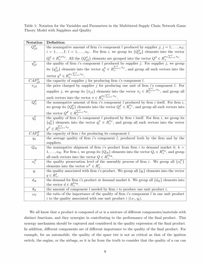
Table 1: Notation for the Variables and Parameters in the Multitiered Supply Chain Network GameTheory Model with Suppliers and Quality
Notation DefinitionQS
jil the nonnegative amount of firm i’s component l produced by supplier j; j = 1, . . . , nS ;i = 1, . . . , I; l = 1, . . . , nli . For firm i, we group its {QS
jil} elements into the vector
QSi ∈ R
nSnli
+ . All the {QSjil} elements are grouped into the vector QS ∈ R
nSPI
i=1 nli
+ .qSjil the quality of firm i’s component l produced by supplier j. For supplier j, we group
its {qSjil} elements into the vector qS
j ∈ RPI
i=1 nli
+ , and group all such vectors into the
vector qS ∈ RnS
PIi=1 nli
+ .CAPS
jil the capacity of supplier j for producing firm i’s component l.πjil the price charged by supplier j for producing one unit of firm i’s component l. For
supplier j, we group its {πjil} elements into the vector πj ∈ RPI
i=1 nli
+ , and group all
such vectors into the vector π ∈ RnS
PIi=1 nli
+ .QF
il the nonnegative amount of firm i’s component l produced by firm i itself. For firm i,we group its {QF
il} elements into the vector QFi ∈ R
nli
+ , and group all such vectors into
the vector QF ∈ RPI
i=1 nli
+ .qFil the quality of firm i’s component l produced by firm i itself. For firm i, we group its
{qFil } elements into the vector qF
i ∈ Rnli
+ , and group all such vectors into the vector
qF ∈ RPI
i=1 nli
+ .CAPF
il the capacity of firm i for producing its component l.qil the average quality of firm i’s component l, produced both by the firm and by the
suppliers.Qik the nonnegative shipment of firm i’s product from firm i to demand market k; k =
1, . . . , nR. For firm i, we group its {Qik} elements into the vector Qi ∈ RnR+ , and group
all such vectors into the vector Q ∈ RInR+ .
αFi the quality preservation level of the assembly process of firm i. We group all {αF
i }elements into the vector αF ∈ RI
+.qi the quality associated with firm i’s product. We group all {qi} elements into the vector
q ∈ RI+.
dik the demand for firm i’s product at demand market k. We group all {dik} elements intothe vector d ∈ RInR
+ .θil the amount of component l needed by firm i to produce one unit product i.ωil the ratio of the importance of the quality of firm i’s component l in one unit product
i to the quality associated with one unit product i (i.e., qi).
We all know that a product is composed of or is a mixture of different components/materials with
distinct functions, and they synergize in contributing to the performance of the final product. This
synergy mechanism should be captured and considered in the quality expression of the final product.
In addition, different components are of different importance to the quality of the final product. For
example, for an automobile, the quality of the spare tire is not as critical as that of the ignition
switch, the engine, or the airbags, so it is far from the truth to consider that the quality of a car can
9

Table 2: Functions for the Multitiered Supply Chain Network Game Theory Model with Suppliersand Quality
Function DefinitionfF
il (QF , qF ) firm i’s production cost for producing its component l; i = 1, . . . , I; l = 1, . . . , nl.fi(Q,αF ) firm i’s cost for assembling its product using the components needed.
tcFik(Q, q) firm i’s transportation cost for shipping its product to demand market k; k =
1, . . . , nR.cijl(QS) the transaction cost paid by firm i for transacting with supplier j; j = 1, . . . , nS , for
its component l.fS
jl(QS , qS) supplier j’s production cost for producing component l.
tcSjil(Q
S , qS) supplier j’s transportation cost for shipping firm i’s component l.
ocjil(π) the opportunity cost of supplier j associated with pricing firm i’s component l atπjil for producing and transporting it.
ρik(d, q) the demand price for firm i’s product at demand market k.
be represented by the quality of the spare tire only because the spare tire is of extremely low or high
quality. Therefore, the weighted summation expression is most general among the three expressions
of product quality in Pennerstorfer and Weiss (2012). Moreover, one should not neglect the fact that,
the quality of a product is also affected by its assembly processes, in which the components should be
fitted together properly in order to achieve particular functions of the product.
Thus, in this paper, we model the quality of a finished product i as a function determined by the
average quality levels of its components, the importance of the quality of the components to the quality
of the product, and the quality preservation level of the assembly process of firm i. It is expressed as:
qi = αFi (
nli∑l=1
ωilqil), i = 1, . . . , I; l = 1. (6)
Note that αFi captures the percentage of the quality preservation of product i in the assembly process
of the firm and lies between 0 and 1, that is:
0 ≤ αFi ≤ 1, i = 1, . . . , I, (7)
where 0 can also be used to represent the value for the quality preservation standard of the assembly
process.
The decay of quality can hence be captured by 1−αFi . In Nagurney and Masoumi (2012), Masoumi,
Yu, and Nagurney (2012), Nagurney and Nagurney (2012), Yu and Nagurney (2013), and in Nagurney
et al. (2013b), arc multipliers that are similar to αFi are used to model the perishability of particular
products, such as pharmaceuticals, human blood, medical nuclear products, and fresh produce, in
terms of the percentages of flows that reach the successor nodes in supply chain networks.
10

We also assume that the importance of the quality levels of all components of product i sums up
to 1, that is:nli∑l=1
ωil = 1, i = 1, . . . , I. (8)
In view of (1), (5), and (6), we can redefine the transportation cost functions of the firms tcFik(Q, q)
and the demand price functions ρik(d, q); i = 1, . . . , I; k = 1, . . . , nR, in quantities and quality levels
of the components, both by the firms and by the suppliers, the quantities of the products, and the
quality preservation levels of the assembly processes, that is:
t̂cFik = t̂c
Fik(Q,QF , QS , qF , qS , αF ) = tcF
ik(Q, q), i = 1, . . . , I; k = 1, . . . , nR, (9)
ρ̂ik = ρ̂ik(Q,QF , QS , qF , qS , αF ) = ρik(d, q), i = 1, . . . , I; k = 1, . . . , nR. (10)
The generality of the expressions in (9) and (10) allows for modeling and application flexibility. The de-
mand price functions (10) are, typically, assumed to be monotonically decreasing in product quantities
but increasing in terms of product quality levels.
As noted in Table 2, the assembly cost functions, the production cost functions, the transportation
cost functions, the transaction cost functions, and the demand price functions are general functions in
vectors of quantities and/or quality levels, since one supplier’s or one firm’s decisions will affect their
competitors’ costs and, hence, their decisions as well. In this way, the interaction among firms and
that among suppliers in their competition for resources and technologies are captured.
Furthermore, the cost functions measure not only the monetary costs in the corresponding pro-
cesses, but also other important factors, such as the time spent in conforming the processes and the
costs of ensuring and assuring quality in these processes (e.g., scrap costs, screening costs, rework
costs, and the investments for quality engineering and training). The compensation costs incurred
when customers are dissatisfied with the quality of the products, such as warranty charges and the
complaint adjustment cost, are also included, which can be utilized to measure the disrepute costs
of the firms. The costs related to quality are all convex functions of quality conformance levels (see,
e.g., Feigenbaum (1983), Juran and Gryna (1988), Campanella (1990), Porter and Rayner (1992), and
Shank and Govindarajan (1994)). In addition, since, as argued by Bender et al. (1985), one of the
most important factors that must be considered in selecting suppliers is their cost, we assume that
the cost functions of the suppliers are known by the firms.
Please note that, since, as mentioned, defectives are hard to define and identify in reality, in the
context of this paper, firms and suppliers may produce defectives. However, they are not motivated
to do so. As reflected in the demand price functions, consumers pay more for products with higher
quality, and, hence, good quality products and components will lead to more revenue. Thus, essentially,
the component quality, the quality preservation/decay level, and hence product quality are highly
dependent on the costs related to quality, the prices of the components, and consumers sensitivity to
product quality.
11

Furthermore, in this paper, we assume that transportation activities affect quality in terms of
quality preservation, and, thus, quality does not deteriorate during transportation, but, as mentioned,
may deteriorate in the assembly processes.
This model is also capable of handling the case of outsourcing by setting each nli ; i = 1, . . . , I, to
1. In such a case, the contractors do the outsourced jobs of producing products and transporting them
to the firms, and the firms do the packaging and labeling for their products and may also produce
in-house. In addition, when the number of firms and the number of the suppliers are one, this model
is able to capture the case of a single firm - single supplier supply chain where the firm procures from
one exclusive supplier, without competition, as in the models in related literature (cf. Section 1 and
Example 1).
2.1 The Behavior of the Firms and Their Optimality Conditions
Given the prices π∗i of the components that the suppliers charge firm i, and the quality qS∗of
the components produced by the suppliers, the objective of firm i; i = 1, . . . , I, is to maximize its
utility/profit UFi . It is the difference between its total revenue and its total cost. The total cost
includes the assembly cost, the production costs, the transportation costs, the transaction costs, and
the payments to the suppliers.Hence, firm i seeks to
MaximizeQi,QFi ,QS
i ,qFi ,αF
iUF
i =nR∑k=1
ρ̂ik(Q,QF , QS , qF , qS∗, αF )dik − fi(Q,αF )−
nli∑l=1
fFil (QF , qF )
−nR∑k=1
t̂cF
ik(Q,QF , QS , qF , qS∗, αF )−
nS∑j=1
nli∑l=1
cijl(QS)−nS∑j=1
nli∑l=1
π∗jilQSjil (11)
subject to:nR∑k=1
Qikθil ≤nS∑j=1
QSjil + QF
il , i = 1, . . . , I; l = 1, . . . , nli , (12)
CAPSjil ≥ QS
jil ≥ 0, j = 1, . . . , nS ; i = 1, . . . , I; l = 1, . . . , nli , (13)
CAPFil ≥ QF
il ≥ 0, i = 1, . . . , I; l = 1, . . . , nli , (14)
and (1), (2), (4), and (7).
We assume that all the cost functions and demand price functions in (11) are continuous and
twice continuously differentiable. The cost functions are convex in quantities and/or quality levels
and have bounded second-order partial derivatives. The demand price functions have bounded first-
order and second-order partial derivatives. Constraint (12) captures the material requirements in the
assembly process. Constraints (13) and (14) indicate that the component production quantities should
be nonnegative and limited by the associated capacities, which can capture the abilities of producing.
If a supplier or a firm is not capable of producing a certain component, the associated capacity should
be 0.
The firms compete in the sense of Nash (1950, 1951). The strategic variables for each firm i are
the product shipments to the demand markets, the in-house component production quantities, the
12
contracted component production quantities, which are produced by the suppliers, the quality levels
of the in-house produced components, and the quality preservation level of its assembly process.
We define the feasible set KFi as K
Fi ≡ {(Qi, Q
Fi , QS
i , qFi , αF
i )|(1), (2), (4), (7), and (12) - (14)
are satisfied}. All KFi ; i = 1, . . . , I, are closed and convex. We also define the feasible set KF ≡
ΠIi=1K
Fi .
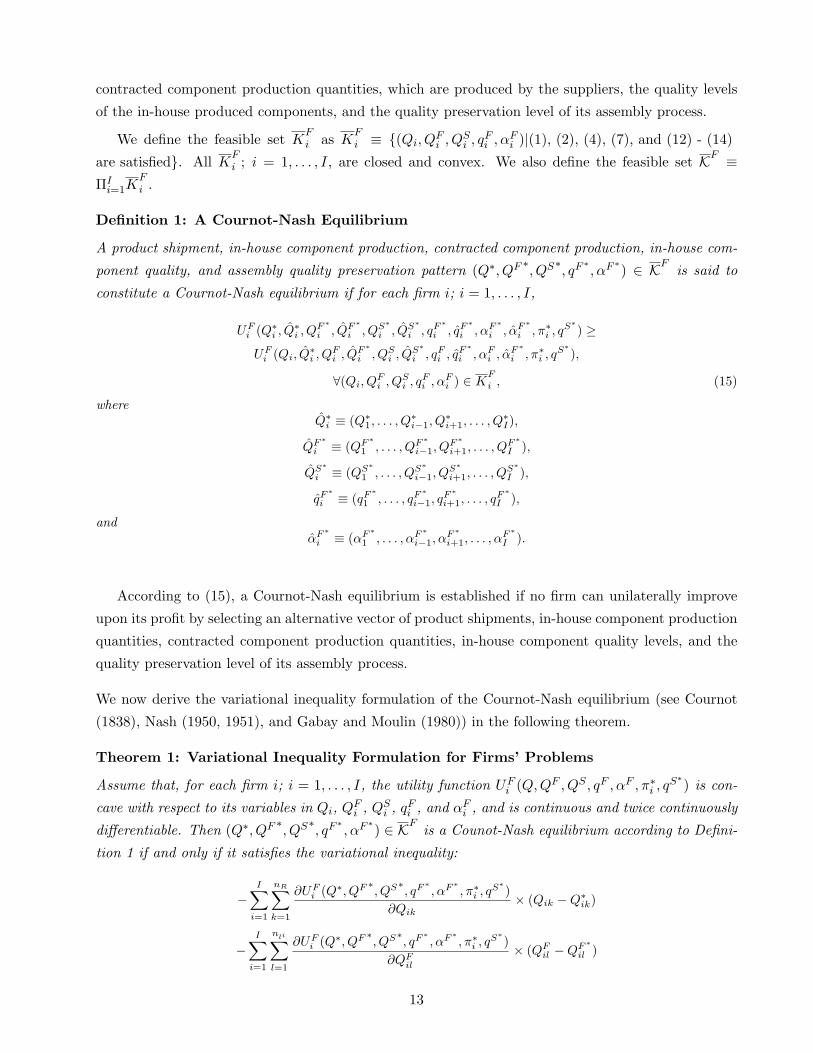
Definition 1: A Cournot-Nash Equilibrium
A product shipment, in-house component production, contracted component production, in-house com-
ponent quality, and assembly quality preservation pattern (Q∗, QF ∗, QS∗, qF ∗
, αF ∗) ∈ KF is said to
constitute a Cournot-Nash equilibrium if for each firm i; i = 1, . . . , I,
UFi (Q∗
i , Q̂∗i , Q
F∗
i , Q̂F∗
i , QS∗
i , Q̂S∗
i , qF∗
i , q̂F∗
i , αF∗
i , α̂F∗
i , π∗i , qS∗) ≥
UFi (Qi, Q̂
∗i , Q
Fi , Q̂F∗
i , QSi , Q̂S∗
i , qFi , q̂F∗
i , αFi , α̂F∗
i , π∗i , qS∗),
∀(Qi, QFi , QS
i , qFi , αF
i ) ∈ KF
i , (15)
whereQ̂∗
i ≡ (Q∗1, . . . , Q
∗i−1, Q
∗i+1, . . . , Q
∗I),
Q̂F∗
i ≡ (QF∗
1 , . . . , QF∗
i−1, QF∗
i+1, . . . , QF∗
I ),
Q̂S∗
i ≡ (QS∗
1 , . . . , QS∗
i−1, QS∗
i+1, . . . , QS∗
I ),
q̂F∗
i ≡ (qF∗
1 , . . . , qF∗
i−1, qF∗
i+1, . . . , qF∗
I ),
andα̂F∗
i ≡ (αF∗
1 , . . . , αF∗
i−1, αF∗
i+1, . . . , αF∗
I ).
According to (15), a Cournot-Nash equilibrium is established if no firm can unilaterally improve
upon its profit by selecting an alternative vector of product shipments, in-house component production
quantities, contracted component production quantities, in-house component quality levels, and the
quality preservation level of its assembly process.
We now derive the variational inequality formulation of the Cournot-Nash equilibrium (see Cournot
(1838), Nash (1950, 1951), and Gabay and Moulin (1980)) in the following theorem.
Theorem 1: Variational Inequality Formulation for Firms’ Problems
Assume that, for each firm i; i = 1, . . . , I, the utility function UFi (Q,QF , QS , qF , αF , π∗i , q
S∗) is con-
cave with respect to its variables in Qi, QFi , QS
i , qFi , and αF
i , and is continuous and twice continuously
differentiable. Then (Q∗, QF ∗, QS∗, qF ∗
, αF ∗) ∈ KF is a Counot-Nash equilibrium according to Defini-
tion 1 if and only if it satisfies the variational inequality:
−I∑
i=1
nR∑k=1
∂UFi (Q∗, QF ∗, QS∗, qF∗
, αF∗, π∗i , qS∗
)∂Qik
× (Qik −Q∗ik)
−I∑
i=1
nli∑l=1
∂UFi (Q∗, QF ∗, QS∗, qF∗
, αF∗, π∗i , qS∗
)∂QF
il
× (QFil −QF∗
il )
13

−nS∑j=1
I∑i=1
nli∑l=1
∂UFi (Q∗, QF ∗, QS∗, qF∗
, αF∗, π∗i , qS∗
)∂QS
jil
× (QSjil −QS∗
jil)
−I∑
i=1
nli∑l=1
∂UFi (Q∗, QF ∗, QS∗, qF∗
, αF∗, π∗i , qS∗
)∂qF
il
× (qFil − qF∗
il )
−I∑
i=1
∂UFi (Q∗, QF ∗, QS∗, qF∗
, αF∗, π∗i , qS∗
)∂αF
i
× (αFi − αF∗
i ) ≥ 0, ∀(Q,QF , QS , qF , αF ) ∈ KF, (16)
with notice that: for i = 1, . . . , I; k = 1, . . . , nR:
−∂UF
i
∂Qik=
"∂fi(Q, αF )
∂Qik+
nRXh=1
∂t̂cFih(Q, QF , QS , qF , qS∗
, αF )
∂Qik−
nRXh=1
∂ρ̂ih(Q, QF , QS , qF , qS∗, αF )
∂Qik× dih
−ρ̂ik(Q, QF , QS , qF , qS∗, αF )
i,
for i = 1, . . . , I; l = 1, . . . , nli :
−∂UF
i
∂QFil
=
24 nliX
m=1
∂fFim(QF , qF )
∂QFil
+
nRXh=1
∂t̂cFih(Q, QF , QS , qF , qS∗
, αF )
∂QFil
−nRXh=1
∂ρ̂ih(Q, QF , QS , qF , qS∗, αF )
∂QFil
× dih
35 ,
for j = 1, . . . , nS; i = 1, . . . , I; l = 1, . . . , nli :
−∂UF
i
∂QSjil
=
24π∗jil +
nSXh=1
nliX
m=1
∂cihm(QS)
∂QSjil
+
nRXh=1
∂t̂cFih(Q, QF , QS , qF , qS∗
, αF )
∂QSjil
−nRXh=1
∂ρ̂ih(Q, QF , QS , qF , qS∗, αF )
∂QSjil
× dih
35 ,
for i = 1, . . . , I; l = 1, . . . , nli :
−∂UF
i
∂qFil
=
24 nliX
m=1
∂fFim(QF , qF )
∂qFil
+
nRXh=1
∂t̂cFih(Q, QF , QS , qF , qS∗
, αF )
∂qFil
−nRXh=1
∂ρ̂ih(Q, QF , QS , qF , qS∗, αF )
∂qFil
× dih
35 ,
for i = 1, . . . , I:
−∂UF
i
∂αFi
=
"∂fi(Q
F , αF )
∂αFi
+
nRXh=1
∂t̂cFih(Q, QF , QS , qF , qS∗
, αF )
∂αFi
−nRXh=1
∂ρ̂ih(Q, QF , QS , qF , qS∗, αF )
∂αFi
× dih
#,
or, equivalently, in view of (1) and (12), (Q∗, QF ∗, QS∗
, qF ∗, αF ∗
, λ∗) ∈ KF is a vector of the equi-
librium product shipment, in-house component production, contracted component production, in-house
component quality, and assembly quality preservation pattern and Lagrange multipliers if and only if
it satisfies the variational inequality
I∑i=1
nR∑k=1
[−∂UF
i (Q∗, QF ∗, QS∗, qF∗, αF∗
, π∗i , qS∗)
∂Qik+
nli∑l=1
λ∗ilθil
]× (Qik −Q∗
ik)
+I∑
i=1
nli∑l=1
[−∂UF
i (Q∗, QF ∗, QS∗, qF∗, αF∗
, π∗i , qS∗)
∂QFil
− λ∗il
]× (QF
il −QF∗
il )
+nS∑j=1
I∑i=1
nli∑l=1
[−∂UF
i (Q∗, QF ∗, QS∗, qF∗, αF∗
, π∗i , qS∗)
∂QSjil
− λ∗il
]× (QS
jil −QS∗
jil)
+I∑
i=1
nli∑l=1
[−∂UF
i (Q∗, QF ∗, QS∗, qF∗, αF∗
, π∗i , qS∗)
∂qFil
]× (qF
il − qF∗
il )
+I∑
i=1
[−∂UF
i (Q∗, QF ∗, QS∗, qF∗, αF∗
, π∗i , qS∗)
∂αFi
]× (αF
i − αF∗
i )
14

+I∑
i=1
nli∑l=1
nS∑j=1
QS∗
jil + QF∗
il −nR∑k=1
Q∗ikθil
× (λil − λ∗il) ≥ 0, ∀(Q,QF , QS , qF , αF , λ) ∈ KF , (17)
where KF ≡ ΠIi=1K
Fi and KF
i ≡ {(Qi, QFi , QS
i , qFi , αF
i , λi)|λi ≥ 0 with (2), (4), (7), (13), and
(14) satisfied}. λi is the nli-dimensional vector with component l being the element λil corresponding
to the Lagrange multiplier associated with the (i, l)-th constraint (12). Both the above-defined feasible
sets are convex.
Proof: Please see the Appendix.
For additional background on the variational inequality problem, please refer to the book by Nagur-
ney (1999).
2.2 The Behavior of the Suppliers and Their Optimality Conditions
Opportunity costs of the suppliers are considered in this model. As in Nagurney, Li, and Nagurney
(2013) and Nagurney and Li (2015), we capture each opportunity cost with a general function that
depends on the entire vector of prices, since the opportunity costs of a supplier may also be affected
by the prices charged by the other suppliers.
Given the QS∗determined by the firms, the objective of supplier j; j = 1, . . . , nS , is to maximize its
total profit, denoted by USj . Its revenue is obtained from the payments of the firms, while its costs are
the costs of production and delivery and the opportunity costs. The strategic variables of a supplier
are the prices that it charges the firms and the quality levels of the components that it produces.
The decision-making problem for supplier j is as the following:
Maximizeπj ,qSj
USj =
I∑i=1
nli∑l=1
πjilQS∗
jil −nl∑
l=1
fSjl(Q
S∗, qS)−
I∑i=1
nli∑l=1
tcSjil(Q
S∗, qS)−
I∑i=1
nli∑l=1
ocjil(π) (18)
subject to:πjil ≥ 0, j = 1, . . . , nS ; i = 1, . . . , I; l = 1, . . . , nli , (19)
and (3).
We assume that the cost functions of each supplier are continuous, twice continuously differentiable,
and convex, and have bounded second-order partial derivatives.
The suppliers compete in a noncooperative in the sense of Nash (1950, 1951), with each one trying
to maximize its own profit. We define the feasible sets KSj ≡ {(πj , q
Sj )|πj ∈ R
PIi=1 nli
+ and qSj sati-
sfies (3) for j}, KS ≡ ΠnSj=1K
Sj , and K ≡ KF ×KS . All the above-defined feasible sets are convex.
Definition 2: A Bertrand-Nash Equilibrium
A price and contracted component quality pattern (π∗, qS∗) ∈ KS is said to constitute a Bertrand-Nash
equilibrium if for each supplier j; j = 1, . . . , nS,
USj (QS∗
, π∗j , π̂∗j , qS∗
j , q̂S∗
j ) ≥ USj (QS∗
, πj , π̂∗j , qS
j , q̂S∗
j ), ∀(πj , qSj ) ∈ KS
j , (20)
15

whereπ̂∗j ≡ (π∗1 , . . . , π∗j−1, π
∗j+1, . . . , π
∗nS
)
andq̂S∗
j ≡ (qS∗
1 , . . . , qS∗
j−1, qS∗
j+1, . . . , qS∗
nS).
According to (20), a Bertrand-Nash equilibrium is established if no supplier can unilaterally improve
upon its profit by selecting an alternative vector of prices that it charges the firms and the quality
levels of the components that it produces.
The variational inequality formulation of the Bertrand-Nash equilibrium according to Definition 2
(see Bertrand (1883), Nash (1950, 1951), Gabay and Moulin (1980), Nagurney (2006)) is given in the
following theorem.
Theorem 2: Variational Inequality Formulation for Suppliers’ Problems
Assume that, for each supplier j; j = 1, . . . , nS, the profit function USj (QS∗
, π, qS) is concave with
respect to the variables in πj and qSj , and is continuous and twice continuously differentiable. Then
(π∗, qS∗) ∈ KS is a Bertrand-Nash equilibrium according to Definition 2 if and only if it satisfies the
variational inequality:
−nS∑j=1
I∑i=1
nli∑l=1
∂USj (QS∗
, π∗, qS∗)
∂πjil× (πjil − π∗jil)−
nS∑j=1
I∑i=1
nli∑l=1
∂USj (QS∗
, π∗, qS∗)
∂qSjil
× (qSjil − qS∗
jil ) ≥ 0,
∀(π, qS) ∈ KS , (21)
with notice that: for j = 1, . . . , nS ; i = 1, . . . , I; l = 1, . . . , nli :
−∂US
j
∂πjil=
IXg=1
nliX
m=1
∂ocjgm(π)
∂πjil− QS∗
jil ,
for j = 1, . . . , nS ; i = 1, . . . , I; l = 1, . . . , nli :
−∂US
j
∂qSjil
=
nlXm=1
∂fSjm(QS∗
, qS)
∂qSjil
+IX
g=1
nliX
m=1
∂tcSjgm(QS∗
, qS)
∂qSjil
.
2.3 The Equilibrium Conditions for the Multitiered Supply Chain Network with Suppliers
and Quality Competition
In equilibrium, the optimality conditions for all firms and the optimality conditions for all suppliers
must hold simultaneously, according to the definition below.
Definition 3: Multitiered Supply Chain Network Equilibrium with Suppliers and Quality
Competition
The equilibrium state of the multitiered supply chain network with suppliers is one where both varia-
tional inequalities (16), or, equivalently, (17), and (21) hold simultaneously.
16

Theorem 3: Variational Inequality Formulation for the Multitiered Supply Chain Net-
work Equilibrium with Suppliers and Quality Competition
The equilibrium conditions governing the multitiered supply chain network model with suppliers and
quality competition are equivalent to the solution of the variational inequality problem: determine
(Q∗, QF ∗, QS∗
, qF ∗, αF ∗
, π∗, qS∗) ∈ K, such that:
−I∑
i=1
nR∑k=1
∂UFi (Q∗, QF ∗, QS∗, qF∗
, αF∗, π∗i , qS∗
)∂Qik
× (Qik −Q∗ik)
−I∑
i=1
nli∑l=1
∂UFi (Q∗, QF ∗, QS∗, qF∗
, αF∗, π∗i , qS∗
)∂QF
il
× (QFil −QF∗
il )
−nS∑j=1
I∑i=1
nli∑l=1
∂UFi (Q∗, QF ∗, QS∗, qF∗
, αF∗, π∗i , qS∗
)∂QS
jil
× (QSjil −QS∗
jil)
−I∑
i=1
nli∑l=1
∂UFi (Q∗, QF ∗, QS∗, qF∗
, αF∗, π∗i , qS∗
)∂qF
il
× (qFil − qF∗
il )
−I∑
i=1
∂UFi (Q∗, QF ∗, QS∗, qF∗
, αF∗, π∗i , qS∗
)∂αF
i
× (αFi − αF∗
i )
−nS∑j=1
I∑i=1
nli∑l=1
∂USj (QS∗
, π∗, qS∗)
∂πjil× (πjil − π∗jil)
−nS∑j=1
I∑i=1
nli∑l=1
∂USj (QS∗
, π∗, qS∗)
∂qSjil
× (qSjil − qS∗
jil ) ≥ 0, ∀(Q,QS , QF , qF , αF , π, qS) ∈ K, (22)
or, equivalently: determine (Q∗, QF∗, QS∗
, qF∗, αF∗
, λ∗, π∗, qS∗) ∈ K, such that:
I∑i=1
nR∑k=1
[−∂UF
i (Q∗, QF ∗, QS∗, qF∗, αF∗
, π∗i , qS∗)
∂Qik+
nli∑l=1
λ∗ilθil
]× (Qik −Q∗
ik)
+I∑
i=1
nli∑l=1
[−∂UF
i (Q∗, QF ∗, QS∗, qF∗, αF∗
, π∗i , qS∗)
∂QFil
− λ∗il
]× (QF
il −QF∗
il )
+nS∑j=1
I∑i=1
nli∑l=1
[−∂UF
i (Q∗, QF ∗, QS∗, qF∗, αF∗
, π∗i , qS∗)
∂QSjil
− λ∗il
]× (QS
jil −QS∗
jil)
+I∑
i=1
nli∑l=1
[−∂UF
i (Q∗, QF ∗, QS∗, qF∗, αF∗
, π∗i , qS∗)
∂qFil
]× (qF
il − qF∗
il )
+I∑
i=1
[−∂UF
i (Q∗, QF ∗, QS∗, qF∗, αF∗
, π∗i , qS∗)
∂αFi
]× (αF
i − αF∗
i )
+I∑
i=1
nli∑l=1
nS∑j=1
QS∗
jil + QF∗
il −nR∑k=1
Q∗ikθil
× (λil − λ∗il)
+nS∑j=1
I∑i=1
nli∑l=1
[−
∂USj (QS∗
, π∗, qS∗)
∂πjil
]× (πjil − π∗jil)
17

+nS∑j=1
I∑i=1
nli∑l=1
[−
∂USj (QS∗
, π∗, qS∗)
∂qSjil
]× (qS
jil − qS∗
jil ) ≥ 0, ∀(Q,QF , QS , qF , αF , λ, π, qS) ∈ K, (23)
where K ≡ KF ×KS.
Proof: Summation of variational inequalities (16) (or (17)) and (21) yields variational inequality (22)
(or (23)). A solution to variational inequality (22) (or (23)) satisfies the sum of (16) (or (17)) and
(21) and, hence, is an equilibrium according to Definition 3.�
We now put variational inequality (23) into standard form (cf. Nagurney (1999)): determine
X∗ ∈ K where X is a vector in RN , F (X) is a continuous function such that F (X) : X 7→ K ⊂ RN ,
and
〈F (X∗), X −X∗〉 ≥ 0, ∀X ∈ K, (24)
where 〈·, ·〉 is the inner product in the N -dimensional Euclidean space, N = InR + 3∑I
i=1 nli +
3nS∑I
i=1 nli + I, and K is closed and convex. We define the vector X ≡ (Q,QF , QS , qF , αF , λ,
π, qS) and the vector F (X) ≡ (F 1(X), F 2(X), F 3(X), F 4(X), F 5(X), F 6(X), F 7(X), F 8(X)), such
that:
F 1(X) =
[−∂UF
i (Q,QF , QS , qF , αF , πi, qS)
∂Qik+
nli∑l=1
λilθil; i = 1, . . . , I; k = 1, . . . , nR
],
F 2(X) =[−∂UF
i (Q,QF , QS , qF , αF , πi, qS)
∂QFil
− λil; i = 1, . . . , I; l = 1, . . . , nli
],
F 3(X) =
[−∂UF
i (Q,QF , QS , qF , αF , πi, qS)
∂QSjil
− λil; j = 1, . . . , nS ; i = 1, . . . , I; l = 1, . . . , nli
],
F 4(X) =[−∂UF
i (Q,QF , QS , qF , αF , πi, qS)
∂qFil
; i = 1, . . . , I; l = 1, . . . , nli
],
F 5(X) =[−∂UF
i (Q,QF , QS , qF , αF , πi, qS)
∂αFi
; i = 1, . . . , I
],
F 6(X) =
nS∑j=1
QSjil + QF
il −nR∑k=1
Qikθil; i = 1, . . . , I; l = 1, . . . , nli
,
F 7(X) =
[−
∂USj (QS , π, qS)
∂πjil; j = 1, . . . , nS ; i = 1, . . . , I; l = 1, . . . , nli
],
F 8(X) =
[−
∂USj (QS , π, qS)
∂qSjil
; j = 1, . . . , nS ; i = 1, . . . , I; l = 1, . . . , nli
]. (25)
Hence, (23) can be put into standard form (24).
Similarly, we also put variational inequality (22) into standard form: determine Y ∗ ∈ K where Y
is a vector in RM , G(Y ) is a continuous function such that G(Y ) : Y 7→ K ⊂ RM , and
〈G(Y ∗), Y − Y ∗〉 ≥ 0, ∀Y ∈ K, (26)
18

where M = InR + 2∑I
i=1 nli + 3nS∑I
i=1 nli + I, and K is closed and convex. We define Y ≡(Q,QF , QS , qF , αF , π, qS), G(Y ) ≡ (− ∂UF
i∂Qik
,−∂UFi
∂QFil
,− ∂UFi
∂QSjil
,−∂UFi
∂qFil
,−∂UFi
∂αFi
,− ∂USj
∂πjil,− ∂US
j
∂qSjil
); j = 1, . . . , nS ; i =
1, . . . , I; l = 1, . . . , nli . Hence, (22) can be put into standard form (26).
The equilibrium solution (Q∗, QF ∗, QS∗
, qF ∗, αF ∗
, π∗, qS∗) to (26) and the (Q∗, QF ∗
, QS∗, qF ∗
,
αF ∗, π∗, qS∗
) in the equilibrium solution to (24) are equivalent for this multitiered supply chain network
problem. In addition to (Q∗, QF ∗, QS∗
, qF ∗, αF ∗
, π∗, qS∗), the equilibrium solution to (24) also contains
the equilibrium Lagrange multipliers (λ∗).
3. Qualitative Properties
In this Section, we present some qualitative properties of the solution to variational inequality (24)
and (26), equivalently, (23) and (22). In particular, we provide the existence result and the uniqueness
result. We also investigate the properties of the function F given by (25) that enters variational
inequality (24) and the function G that enters variational inequality (26).
In a multitiered supply chain network with suppliers, it is reasonable to expect that the price
charged by each supplier j for producing one unit of firm i’s component l, πjil, is bounded by a
sufficiently large value, since, in practice, each supplier cannot charge unbounded prices to the firms.
Therefore, the following assumption is not unreasonable:
Assumption 1
Suppose that in our multitiered supply chain network model with suppliers and quality competition,
there exist a sufficiently large Π, such that,
πjil ≤ Π, j = 1, . . . , nS ; i = 1, . . . , I; l = 1, . . . , nli . (27)
With this assumption, we have the following existence result.
Theorem 4: Existence
With Assumption 1 satisfied, there exists at least one solution to variational inequality (24) and (26),
equivalently, (23) and (22).
Proof : Please see the Appendix.
Theorem 5: Monotonicity
Under the assumptions in Theorems 1 and 2, the F (X) that enters variational inequality (24), is
monotone, that is,
〈F (X ′)− F (X ′′), X ′ −X ′′〉 ≥ 0, ∀X ′, X ′′ ∈ K, (28)
and the G(Y ) that enters variational inequality (27) is also monotone,
〈G(Y ′)−G(Y ′′), Y ′ − Y ′′〉 ≥ 0, ∀Y ′, Y ′′ ∈ K. (29)
19

Proof : Please see the Appendix.
Definition 4: Strict Monotonicity
The function G(Y ) in variational inequality (26) is strictly monotone on K̄ if
〈G(Y ′)−G(Y ′′), Y ′ − Y ′′〉 > 0, ∀Y ′, Y ′′ ∈ K̄, Y ′ 6= Y ′′. (30)
The monotonicity of the function G is closely related to the positive-definiteness of its Jacobian
∇G (cf. Nagurney (1999)). Particularly, if ∇G is positive-definite, G is strictly monotone.
Theorem 6: Uniqueness
Assume that the strict monotonicity condition (30) is satisfied. Then, if variational inequality (26)
admits a solution, (Q∗, QF ∗, QS∗
, qF ∗, αF ∗
, π∗, qS∗), that is the only solution.
Proof : Under the strict monotonicity assumption given by (30), the proof follows the standard
variational inequality theory (cf. Kinderlehrer and Stampacchia (1980)). �
Theorem 7: Lipschitz Continuity
The function that enters the variational inequality problem (24) is Lipschitz continuous, that is,
‖ F (X ′)− F (X ′′) ‖≤ L ‖ X ′ −X ′′ ‖, ∀X ′, X ′′ ∈ K, where L > 0. (31)
Proof : Since we have assumed that all the cost functions have bounded second-order partial deriva-
tives, and the demand price functions have bounded first-order and second-order partial derivatives,
the result is direct by applying a mid-value theorem from calculus to the F (X) that enters variational
inequality (24). �
4. The Algorithm
We employ the modified projection method (see Korpelevich (1997) and Nagurney (1999)) for the
computation of the solution for the multitiered supply chain network game theory model with suppliers
and quality competition. It has been effectively used in large-scale supply chain network equilibrium
problems (cf. Liu and Nagurney (2009)). The statement of the modified projection method is as
follows, where T denotes an iteration counter:
The Modified Projection Method
Step 0: Initialization
Start with X0 ∈ K (cf. (24)). Set T := 1 and select a, such that 0 < a ≤ 1L , where L is the Lipschitz
continuity constant (cf. 31) for F (X) (cf. (24))
20
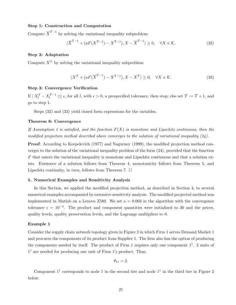
Step 1: Construction and Computation
Compute XT −1 by solving the variational inequality subproblem:
〈XT −1 + (aF (XT −1)−XT −1), X −XT −1〉 ≥ 0, ∀X ∈ K. (32)
Step 2: Adaptation
Compute XT by solving the variational inequality subproblem:
〈XT + (aF (XT −1)−XT −1), X −XT 〉 ≥ 0, ∀X ∈ K. (33)
Step 3: Convergence Verification
If | XTl −XT −1
l |≤ ε, for all l, with ε > 0, a prespecified tolerance, then stop; else set T := T + 1, and
go to step 1.
Steps (32) and (33) yield closed form expressions for the variables.
Theorem 8: Convergence
If Assumption 1 is satisfied, and the function F (X) is monotone and Lipschitz continuous, then the
modified projection method described above converges to the solution of variational inequality (24).
Proof: According to Korpelevich (1977) and Nagurney (1999), the modified projection method con-
verges to the solution of the variational inequality problem of the form (24), provided that the function
F that enters the variational inequality is monotone and Lipschitz continuous and that a solution ex-
ists. Existence of a solution follows from Theorem 4, monotonicity follows from Theorem 5, and
Lipschitz continuity, in turn, follows from Theorem 7. �
5. Numerical Examples and Sensitivity Analysis
In this Section, we applied the modified projection method, as described in Section 4, to several
numerical examples accompanied by extensive sensitivity analysis. The modified projected method was
implemented in Matlab on a Lenovo Z580. We set a = 0.003 in the algorithm with the convergence
tolerance ε = 10−4. The product and component quantities were initialized to 30 and the prices,
quality levels, quality preservation levels, and the Lagrange multipliers to 0.
Example 1
Consider the supply chain network topology given in Figure 2 in which Firm 1 serves Demand Market 1
and procures the components of its product from Supplier 1. The firm also has the option of producing
the components needed by itself. The product of Firm 1 requires only one component 11. 2 units of
11 are needed for producing one unit of Firm 1’s product. Thus,
θ11 = 2.
Component 11 corresponds to node 1 in the second tier and node 11 in the third tier in Figure 2
below.
21

j1Demand Market?
j1′?j1Firm
HH
HHHj?
j111j
Supplier 1j?
Figure 2: Supply Chain Network Topology for Example 1
The data are as follows.
The capacity of the supplier is:
CAPS111 = 120.
The firm’s capacity for producing its component is:
CAPF11 = 80.
The value that represents the perfect component quality is:
q̄11 = 75.
The supplier’s production cost is:
fS11(Q
S111, q
S111) = 5QS
111 + 0.8(qS111 − 62.5)2.
The supplier’s transportation cost is:
tcS111(Q
S111, q
S111) = 0.5QS
111 + 0.2(qS111 − 125)2 + 0.3QS
111qS111,
and its opportunity cost is:
oc111(π111) = 0.7(π111 − 100)2.
The firm’s assembly cost is:
f1(Q11, αF1 ) = 0.75Q2
11 + 200αF 2
1 + 200αF1 + 25Q11α
F1 .
The firm’s production cost for producing its component is:
fF11(Q
F11, q
F11) = 2.5QF 2
11 + 0.5(qF11 − 60)2 + 0.1QF
11qF11,
22

and its transaction cost is:
c111(QS111) = 0.5QS2
111 + QS111 + 100.
The firm’s transportation cost for shipping its product to the demand market is:
tcF11(Q11, q1) = 0.5Q2
11 + 0.02q21 + 0.1Q11q1,
and the demand price function at Demand Market 1 is:
ρ11(d11, q1) = −d11 + 0.7q1 + 1000,
where q1 = αF1 ω11
QF11qF
11+QS111qS
111
QF11+QS
111and ω11 = 1.
The equilibrium solution that we obtain using the modified projection method is:
Q∗11 = 89.26, QF∗
11 = 60.16, QS∗
111 = 118.38, qF∗
11 = 71.17,
qS∗
111 = 57.25, π∗11 = 184.53, αF∗
1 = 1.00, λ∗11 = 305.25.
with the induced demand, demand price, and product quality being
d11 = 89.26, ρ11 = 954.10, q1 = 61.94.
The profit of the firm is 33,331.69, and the profit of the supplier is 13,218.67.
For this example, the eigenvalues of the symmetric part of the Jacobian matrix of G(Y ∗) (cf. (27))
are 0.0016, 0.0101, 0.0140, 0.0169, 0.0439, 0.0503, 5.5468, which are all positive. Therefore, ∇G(Y ∗)
is positive-definite, and G(Y ∗) is locally strictly monotone at Y ∗.
Sensitivity Analysis
In Example 1, the capacities of the firm and the supplier do not constrain the production of the
components, since, at the equilibrium, the component quantities are lower than the associated capac-
ities. However, in some cases, due to disruptions to capacities, such as disasters and strikes, firms
and suppliers may not always be able to operate under desired capacities. In this sensitivity analysis,
we investigate the impacts of the capacities that constrain the production of the components on the
quantities, prices, quality levels, and the profits of the firm and the supplier.
First, we maintain the capacity of the firm at 80, and vary the capacity of the supplier from 0 to
20, 40, 60, 80, 100, and 120. The results of equilibrium quantities, quality levels, prices, and profits
are shown in Figures 3 and 4.
As indicated in Figure 3.b, when the capacity of the supplier is 0, the firm has to produce the
components for its product by itself, at full capacity, which is 80. This production pressure limits the
firm’s ability to produce with high quality, which causes a low in-house component quality (cf. Figure
3.d). Based on the data in this example, purchasing components from the supplier is always cheaper
than producing them in-house. Therefore, as the capacity of the supplier increases, the firm buys
more components from the supplier and tends to be more dependent on the supplier in component
production.
23

Figure 3: Equilibrium Component Quantities, Equilibrium Component Quality Levels, EquilibriumProduct Quantity (Demand), and Product Quality as the Capacity of the Supplier Varies
24

Figure 4: Equilibrium Quality Preservation Level, Equilibrium Lagrange Multiplier, Demand Price,Equilibrium Contracted Price, the Supplier’s Profit, and the Firm’s Profit as the Capacity of theSupplier Varies
25
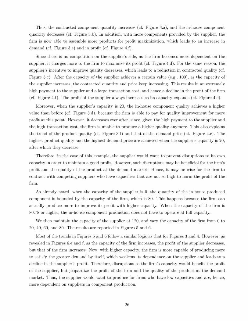
Thus, the contracted component quantity increases (cf. Figure 3.a), and the in-house component
quantity decreases (cf. Figure 3.b). In addition, with more components provided by the supplier, the
firm is now able to assemble more products for profit maximization, which leads to an increase in
demand (cf. Figure 3.e) and in profit (cf. Figure 4.f).
Since there is no competition on the supplier’s side, as the firm becomes more dependent on the
supplier, it charges more to the firm to maximize its profit (cf. Figure 4.d). For the same reason, the
supplier’s incentive to improve quality decreases, which leads to a reduction in contracted quality (cf.
Figure 3.c). After the capacity of the supplier achieves a certain value (e.g., 100), as the capacity of
the supplier increases, the contracted quantity and price keep increasing. This results in an extremely
high payment to the supplier and a large transaction cost, and hence a decline in the profit of the firm
(cf. Figure 4.f). The profit of the supplier always increases as its capacity expands (cf. Figure 4.e).
Moreover, when the supplier’s capacity is 20, the in-house component quality achieves a higher
value than before (cf. Figure 3.d), because the firm is able to pay for quality improvement for more
profit at this point. However, it decreases ever after, since, given the high payment to the supplier and
the high transaction cost, the firm is unable to produce a higher quality anymore. This also explains
the trend of the product quality (cf. Figure 3.f) and that of the demand price (cf. Figure 4.c). The
highest product quality and the highest demand price are achieved when the supplier’s capacity is 20,
after which they decrease.
Therefore, in the case of this example, the supplier would want to prevent disruptions to its own
capacity in order to maintain a good profit. However, such disruptions may be beneficial for the firm’s
profit and the quality of the product at the demand market. Hence, it may be wise for the firm to
contract with competing suppliers who have capacities that are not so high to harm the profit of the
firm.
As already noted, when the capacity of the supplier is 0, the quantity of the in-house produced
component is bounded by the capacity of the firm, which is 80. This happens because the firm can
actually produce more to improve its profit with higher capacity. When the capacity of the firm is
80.78 or higher, the in-house component production does not have to operate at full capacity.
We then maintain the capacity of the supplier at 120, and vary the capacity of the firm from 0 to
20, 40, 60, and 80. The results are reported in Figures 5 and 6.
Most of the trends in Figures 5 and 6 follow a similar logic as that for Figures 3 and 4. However, as
revealed in Figures 6.e and f, as the capacity of the firm increases, the profit of the supplier decreases,
but that of the firm increases. Now, with higher capacity, the firm is more capable of producing more
to satisfy the greater demand by itself, which weakens its dependence on the supplier and leads to a
decline in the supplier’s profit. Therefore, disruptions to the firm’s capacity would benefit the profit
of the supplier, but jeopardize the profit of the firm and the quality of the product at the demand
market. Thus, the supplier would want to produce for firms who have low capacities and are, hence,
more dependent on suppliers in component production.
26

Figure 5: Equilibrium Component Quantities, Equilibrium Component Quality Levels, EquilibriumProduct Quantity (Demand), and Product Quality as the Capacity of the Firm Varies
27
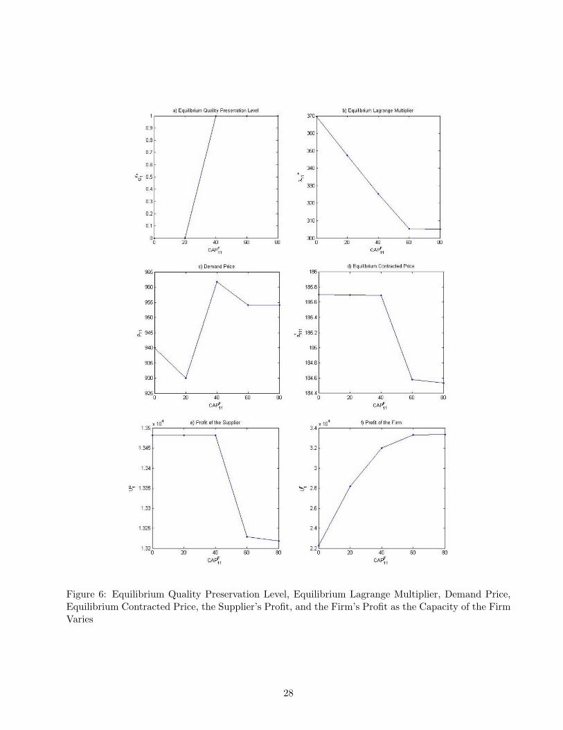
Figure 6: Equilibrium Quality Preservation Level, Equilibrium Lagrange Multiplier, Demand Price,Equilibrium Contracted Price, the Supplier’s Profit, and the Firm’s Profit as the Capacity of the FirmVaries
28

As shown in Figure 5.a, when the capacity of the firm is 0, 20, and 40, the quantity of contracted
component production is bounded by the capacity of the supplier. Actually, when the capacity of the
supplier is no less than 141.71, 133.99, and 126.20, respectively, the supplier does not need to operate
at full capacity.
Investing in Capacity Changing
This sensitivity analysis further sheds light on the investments in capacity changing for the supplier
and for the firm. If the investment is higher than the associated profit improvement, it is not wise
for the supplier or the firm to invest in themselves’ or each other’s capacity changing. Tables 3 and
4 below show the maximum acceptable investments for capacity changing for this sensitivity analysis.
The first number in each cell is the maximum acceptable investment for the supplier, and the second
is that for the firm. In the italic cells, the two numbers are with different signs.
In Tables 3 and 4, for the cells in which both numbers are negative, it is not wise for the firm or
the supplier to change the capacities at all, because their profits would decrease with the associated
capacity change. For the italic cells that are with two opposite-sign numbers, the one with the negative
number should prevent the other from investing in the associated capacity change, or, it should ask
the other for a compensation which will prevent its profit from being compromised. This situation
may occur only in 4 cases when the supplier’s capacity varies (cf. Table 3). However, in Table 4, it
happens very often when the firm’s capacity varies, which is consistent with the results in the above
sensitivity analysis. For the numbers that are 0, the associated profits will not be affected by the
corresponding capacity changes.
In addition, if there is a capacity changing offer that costs more than the summation of the two
numbers in the associated cell, it is not worthwhile for the supplier or the firm to accept the offer,
since more profit cannot be obtained by doing so. If the offer costs less, the two parties should consider
investing in the associated capacity change, and, if possible, negotiate on the separation of the payment
between themselves.
Table 3: Maximum Acceptable Investments (×103) for Capacity Changing when the Capacity of theFirm Maintains 80 but that of the Supplier Varies
PPPPPPFromTo
CAP S111=0 20 40 60 80 100 120
CAP S111=0 – 0.97, 5.89 2.86, 10.17 5.08, 13.09 7.57, 14.62 10.37, 14.77 13.22, 13.6920 -0.97, -5.89 – 1.90, 4.28 4.09, 7.20 6.60, 8.73 9.40, 8.88 12.25, 7.8040 -2.86, -10.17 -1.90, -4.28 – 2.20, 2.92 4.70, 4.45 7.51, 4.60 10.36, 3.5260 -5.06, -13.09 -4.09, -7.20 -2.20, -2.92 – 2.50, 1.53 5.31, 1.68 8.16, 0.6080 -7.57, -14.62 -6.60, -8.73 -4.70, -4.45 -2.50, -1.53 – 2.81, 0.15 5.66, -0.93100 -10.37, -14.77 -9.40, -8.88 -7.51, -4.60 -5.31, -1.68 -2.81, -0.15 – 2.85, -1.08120 -13.22, -13.69 -12.25, -7.80 -10.36, -3.52 -8.16, -0.60 -5.65, 0.93 -2.85, 1.08 –
Example 2
In Example 2, there are 2 firms competing with each other with differentiated but substitutable
products in Demand Market 1. The firms can procure the components for producing their products
29

Table 4: Maximum Acceptable Investments (×103) for Capacity Changing when the Capacity of theSupplier Maintains 120 but that of the Firm Varies
PPPPPPFromTo
CAP F11=0 20 40 60 80
CAP F11=0 – 0.00, 5.94 0.00, 9.77 -0.25, 11.10 -0.26, 11.10
20 0.00, -5.94 – 0.00, 3.83 -0.25, 5.16 -0.26, 5.1640 0.00, -9.77 0.00, -3.83 – -0.25, 1.33 -0.26, 1.3360 0.25, -11.10 0.25, -5.16 0.25, -1.33 – -0.01, 0.00480 0.26, -11.10 0.26, -5.16 0.26, -1.33 0.01, -0.004 –
from Suppliers 1 and 2 who also compete noncooperatively, and they can also produce the components
needed by themselves.
Two components are required by the product of Firm 1, components 11 and 21. 1 unit of 11 and
2 units of 21 are required for producing 1 unit of Firm 1’s product. In order to produce 1 unit Firm
2’s product, 2 units of 12 and 1 unit of 12 are needed. Therefore,
θ11 = 1, θ12 = 2, θ21 = 2, θ22 = 1.
The ratio of the importance of the quality of the components to the quality of one unit product is:
ω11 = 0.2, ω12 = 0.8, ω21 = 0.4, ω22 = 0.6.
The network topology of Example 2 is as in Figure 7. Components 11 and 21 are the same
component, which correspond to nodes 1’s in the second tier of the figure. Components 21 and 22 are
the same component, and they correspond to nodes 2’s in the second tier.
l1Demand Market
@@
@@R
��
��
l1′ 2′l? ?
l1Firms 2lHH
HHHHj? ?
�������
1l l2 1l l2�
��
��
��
\\
\\
\\
\
�������������
HHHHHHHHHHHHH
11l 21l l12 l22XXXXXXXXXXX
�����������
ll
ll
ll
ll
,,
,,
,,
,, R)Uq q�)
��
�
@@@R
��
�
@@@R
l1 l2Suppliers
Figure 7: Supply Chain Network Topology for Example 2
The other data are as follows:
30

The capacities of the suppliers are:
CAPS111 = 80, CAPS
112 = 100, CAPS121 = 100, CAPS
122 = 60,
CAPS211 = 60, CAPS
212 = 100, CAPS221 = 100, CAPS
222 = 50.
The firms’ capacities for in-house component production are:
CAPF11 = 30, CAPF
12 = 30, CAPF21 = 30, CAPF
22 = 30.
The values representing the perfect component quality are:
q̄11 = 60, q̄12 = 75, q̄21 = 60, q̄22 = 75.
The suppliers’ production costs are:
fS11(Q
S111, Q
S121, q
S111, q
S121, q
S211, q
S221) = 0.4(QS
111 + QS121) + 1.5(qS
111 − 50)2 + 1.5(qS121 − 50)2 + qS
211 + qS221,
fS12(Q
S112, Q
S122, q
S112, q
S122, q
S212, q
S222) = 0.4(QS
112 + QS122) + 2(qS
112 − 45)2 + 2(qS122 − 45)2 + qS
212 + qS222,
fS21(Q
S211, Q
S221, q
S211, q
S221, q
S111, q
S121) = QS
211 + QS221 + 2(qS
211 − 31.25)2 + 2(qS221 − 31.25)2 + qS
111 + qS121,
fS12(Q
S212, Q
S222, q
S212, q
S222, q
S112, q
S122) = QS
212 + QS222 + (qS
212 − 85)2 + (qS222 − 85)2 + qS
112 + qS122.
Their transportation costs are:
tcS111(Q
S111, q
S111) = 0.2QS
111 + 1.2(qS111 − 41.67)2, tcS
112(QS112, q
S112) = 0.1QS
112 + 1.2(qS112 − 37.5)2,
tcS121(Q
S121, q
S121) = 0.2QS
121 + 1.4(qS121 − 39.29)2, tcS
122(QS122, q
S122) = 0.1QS
122 + 1.1(qS122 − 36.36)2,
tcS211(Q
S211, q
S211) = 0.3QS
211 + 1.3(qS211 − 30.77)2, tcS
212(QS212, q
S212) = 0.4QS
212 + 1.7(qS212 − 32.35)2,
tcS221(Q
S221, q
S221) = 0.2QS
221 + 1.3(qS221 − 30.77)2, tcS
222(QS222, q
S222) = 0.1QS
222 + 1.5(qS222 − 30)2.
The opportunity costs of the suppliers are:
oc111(π111, π211) = 5(π111 − 80)2 + 0.5π211, oc112(π112, π212) = 9(π112 − 80)2 + π212,
oc121(π121, π221) = 5(π121 − 100)2 + π221, oc122(π122, π222) = 7.5(π122 − 50)2 + 0.1π222,
oc211(π211, π111) = 5(π211 − 50)2 + 2π111, oc212(π212, π112) = 8(π212 − 70)2 + 0.5π112,
oc221(π221, π121) = 9(π221 − 60)2 + π121, oc222(π222, π122) = 8(π222 − 60)2 + 0.5π122.
The firms’ assembly costs are:
f1(Q11, αF1 ) = 3Q2
11 + 0.5Q11αF1 + 100αF 2
1 + 50αF1 ,
f2(Q21, αF2 ) = 2.75Q2
21 + 0.6Q21αF2 + 100αF 2
2 + 50αF2 .
Their production costs for producing components are:
fF11(Q
F11, q
F11) = QF 2
11 + 0.0001QF11q
F11 + 1.1(qF
11 − 36.36)2,
31

fF12(Q
F12, q
F12) = 1.25QF 2
12 + 0.0001QF12q
F12 + 1.2(qF
12 − 41.67)2,
fF21(Q
F21, q
F21) = QF 2
21 + 0.0001QF21q
F21 + 1.5(qF
21 − 33.33)2,
fF22(Q
F22, q
F22) = 0.75QF 2
22 + 0.0001QF22q
F22 + 1.25(qF
22 − 36)2.
The transaction costs are:
c111(QS111) = 0.5QS2
111 + QS111 + 100, c112(QS
112) = 0.5QS2
112 + 0.5QS112 + 150,
c121(QS211) = 0.75QS2
211 + 0.75QS211 + 150, c122(QS
212) = QS2
212 + QS212 + 100,
c211(QS121) = 0.75QS2
121 + QS121 + 150, c212(QS
122) = 0.5QS2
122 + 0.75QS122 + 100,
c221(QS221) = 0.8QS2
221 + 0.25QS221 + 100, c222(QS
222) = 0.5QS2
222 + QS222 + 175.
The firms’ transportation costs are:
tcF11(Q11, q1) = 3Q2
11 + 0.3Q11q1 + 0.25q1, tcF21(Q21, q2) = 3Q2
21 + 0.3Q21q2 + 0.1q2,
and the demand price functions are:
ρ11(d11, d21, q1, q2) = −3d11 − 1.3d21 + q1 + 0.74q2 + 2200,
ρ21(d21, d11, q2, q1) = −3.5d21 − 1.4d11 + 1.1q2 + 0.9q1 + 1800,
where q1 = αF1 (ω11
QF11qF
11+QS111qS
111+QS211qS
211QF
11+QS111+QS
211+ ω12
QF12qF
12+QS112qS
112+QS212qS
212QF
12+QS112+QS
212) and q2 = αF
2 (ω21
QF21qF
21+QS121qS
121+QS221qS
221QF
21+QS121+QS
221+ ω22
QF22qF
22+QS122qS
122+QS222qS
222QF
22+QS122+QS
222).
The modified projection method converges to the following equilibrium solution:
Q∗11 = 93.56, Q∗
21 = 71.34,
QF∗
11 = 30.00, QF∗
12 = 30.00, QF∗
21 = 30.00, QF∗
22 = 30.00,
QS∗
111 = 27.37, QS∗
112 = 100.00, QS∗
121 = 45.44, QS∗
122 = 23.35,
QS∗
211 = 36.19, QS∗
212 = 57.12, QS∗
221 = 67.24, QS∗
222 = 17.99,
qF∗
11 = 38.26, qF∗
12 = 45.15, qF∗
21 = 34.93, qF∗
22 = 41.71,
qS∗
111 = 46.30, qS∗
112 = 42.19, qS∗
121 = 44.83, qS∗
122 = 41.94,
qS∗
211 = 31.06, qS∗
212 = 51.85, qS∗
221 = 31.06, qS∗
222 = 52.00,
π∗111 = 82.74, π∗112 = 85.56, π∗121 = 104.54, π∗122 = 51.56,
π∗211 = 53.62, π∗212 = 73.57, π∗221 = 63.74, π∗222 = 61.12,
αF∗
1 = 1.00, αF∗
2 = 1.00,
λ∗11 = 109.83, λ∗12 = 187.06, λ∗21 = 172.34, λ∗22 = 76.58,
and the induced demands, demand prices, and product quality levels are:
d11 = 93.56, d21 = 71.34, ρ11 = 1, 901.07, ρ21 = 1, 504.22,
q1 = 44.06, q2 = 41.13.
The firms’ profits are 94,610.69 and 57,787.69, respectively, and those of the suppliers are 15,671.13
and 6923.20.
32

The eigenvalues of the symmetric part of the Jacobian matrix of G(Y ) (cf. (27)) are 0.0089, 0.0098,
0.0100, 0.0102, 0.0107, 0.0135, 0.0147, 0.0151, 0.0158, 0.0164, 0.0198, 0.0198, 0.0201, 0.0224, 0.0254,
0.0298, 0.0409, 0.0492, 0.0540, 0.0564, 0.0578, 0.0605, 0.0650, 0.0660, 0.1000, 0.1000, 0.1000, 0.1063,
0.1500, 0.1600, 0.1600, 0.1600, 0.1800, 0.1800, 2.0280, 2.1399, which are all positive. Thus, G(Y ∗) is
locally strictly monotone at Y ∗.
Supplier Disruption Analysis and the Values of Suppliers
As mentioned in the Introduction, the manufacturing plants of suppliers may be located in different
geographical locations around the globe, which increases the vulnerability of the supply chain networks
of the firms to the disruptions that happen to the suppliers, such as those caused by natural disasters.
In this analysis, we model and analyze the impacts of the disruptions to Suppliers 1 and 2 on the
profits of the firms and the demands, prices, and quality levels of the products.
We also evaluate the values of the two suppliers and which one of them is more important to the
firms. With the values of the suppliers and the importance level of them to the firms, the firms can
make more specific and targeted efforts in their supplier management strategies and in the contingency
plans in handling the disruptions to their suppliers.
First, we present the following disruption. The data are as in Example 2, except that Supplier 1 is
no longer available for the firms to contract with or to produce or transport the components needed.The equilibrium solution achieved by the modified projection method is:
Q∗11 = 65.00, Q∗
21 = 65.00,
QF∗
11 = 30.00, QF∗
12 = 30.00, QF∗
21 = 30.00, QF∗
22 = 30.00,
QS∗
111 = 0.00, QS∗
112 = 0.00, QS∗
121 = 0.00, QS∗
122 = 0.00,
QS∗
211 = 35.00, QS∗
212 = 100.00, QS∗
221 = 100.00, QS∗
222 = 35.00,
qF∗
11 = 38.26, qF∗
12 = 45.16, qF∗
21 = 34.93, qF∗
22 = 41.75,
qS∗
211 = 31.06, qS∗
212 = 51.85, qS∗
221 = 31.06, qS∗
222 = 52.00,
π∗211 = 53.50, π∗212 = 76.25, π∗221 = 65.56, π∗222 = 62.19,
αF∗
1 = 1.00, αF∗
2 = 1.00,
λ∗11 = 107.53, λ∗12 = 448.93, λ∗21 = 242.02, λ∗22 = 95.98,
and the induced demands, demand prices, and product quality levels are:
d11 = 65.00, d21 = 65.00 ρ11 = 1, 998.07, ρ21 = 1, 569.17,
q1 = 47.12, q2 = 41.14.
The firms’ profits are 80,574.83 and 57,406.47, respectively, and Supplier 2’s profit is 13,635.49.
Without Supplier 1 and with the firms’ limited in-house production capacities, there is no competi-
tion on the suppliers’ side and the firms have to depend more on the supplier in component production.
Therefore, as shown by the results, 3 out of the 4 contracted component quantities produced by Sup-
plier 2 increase. Supplier 2 charges the firms more than before, and its profit improves. Without
Supplier 1, the firms are not able to provide as many products as before, and hence, the demands at
33

the demand market decrease. The quality of the products of Firms 1 and 2 increase, and the prices
at the demand market increase.
Under this disruption, the profit of Firm 1 decreases by 14.84%, and that of Firm 2 decreases by
0.66%. Therefore, from this perspective, Supplier 1 is more important to Firm 1 than to Firm 2. The
value of Supplier 1 to Firm 1 is 14,035.86, and that to Firm 2 is 381.22, which are measured by the
associated profit declines.
We then present the disruption in which Supplier 2 is no longer available to the firms. The other
data are the same as in Example 2.The modified projection method converges to the following equilibrium solution:
Q∗11 = 65.00, Q∗
21 = 63.79,
QF∗
11 = 30.00, QF∗
12 = 30.00, QF∗
21 = 30.00, QF∗
22 = 30.00,
QS∗
111 = 35.00, QS∗
112 = 100.00, QS∗
121 = 97.58, QS∗
122 = 33.79,
QS∗
211 = 0.00, QS∗
212 = 0.00, QS∗
221 = 0.00, QS∗
222 = 0.00,
qF∗
11 = 38.26, qF∗
12 = 45.16, qF∗
21 = 34.93, qF∗
22 = 41.75,
qS∗
111 = 46.30, qS∗
112 = 42.19, qS∗
121 = 44.83, qS∗
122 = 41.94,
π∗111 = 83.50, π∗112 = 85.56, π∗121 = 109.76, π∗122 = 52.25,
αF∗
1 = 1.00, αF∗
2 = 1.00,
λ∗11 = 119.17, λ∗12 = 442.79, λ∗21 = 256.75, λ∗22 = 86.75.
The induced demands, demand prices, and product quality levels are:
d11 = 65.00, d21 = 63.79, ρ11 = 1, 996.05, ρ21 = 1, 570.59,
q1 = 42.82, q2 = 42.11.
The firms’ profits are 83,895.42 and 53,610.96, respectively, and Supplier 1’s profit is 22,729.18.
The impacts of the disruption to Supplier 2 follow similar logic as those brought about by the
disruption to Supplier 1. The contracted component quantities by Supplier 1 increase, and its profit
increases. The demands at the demand market decrease. Firm 1’s product quality decreases, and
Firm 2’s increases. The prices at the demand market increase.
Without Supplier 2, Firm 1’s profit declines by 11.33%, and that of Firm 2 reduces by 7.23%.
Thus, Supplier 2 is more important to Firm 1 than to Firm 2 under this disruption. The value of
Supplier 2 to Firm 1 is 10,715.27, and that to Firm 2 is 4,176.73.
In addition, according to the above results, Supplier 1 is more important than Supplier 2 to Firm
1, and to Firm 2, Supplier 2 is more important.
For completeness, the disruption in which neither of the supplier is no longer available to the firms
is also considered. The other data are the same as in Example 2.The equilibrium solution obtained using the modified projection method is:
Q∗11 = 15.00, Q∗
21 = 15.00,
34
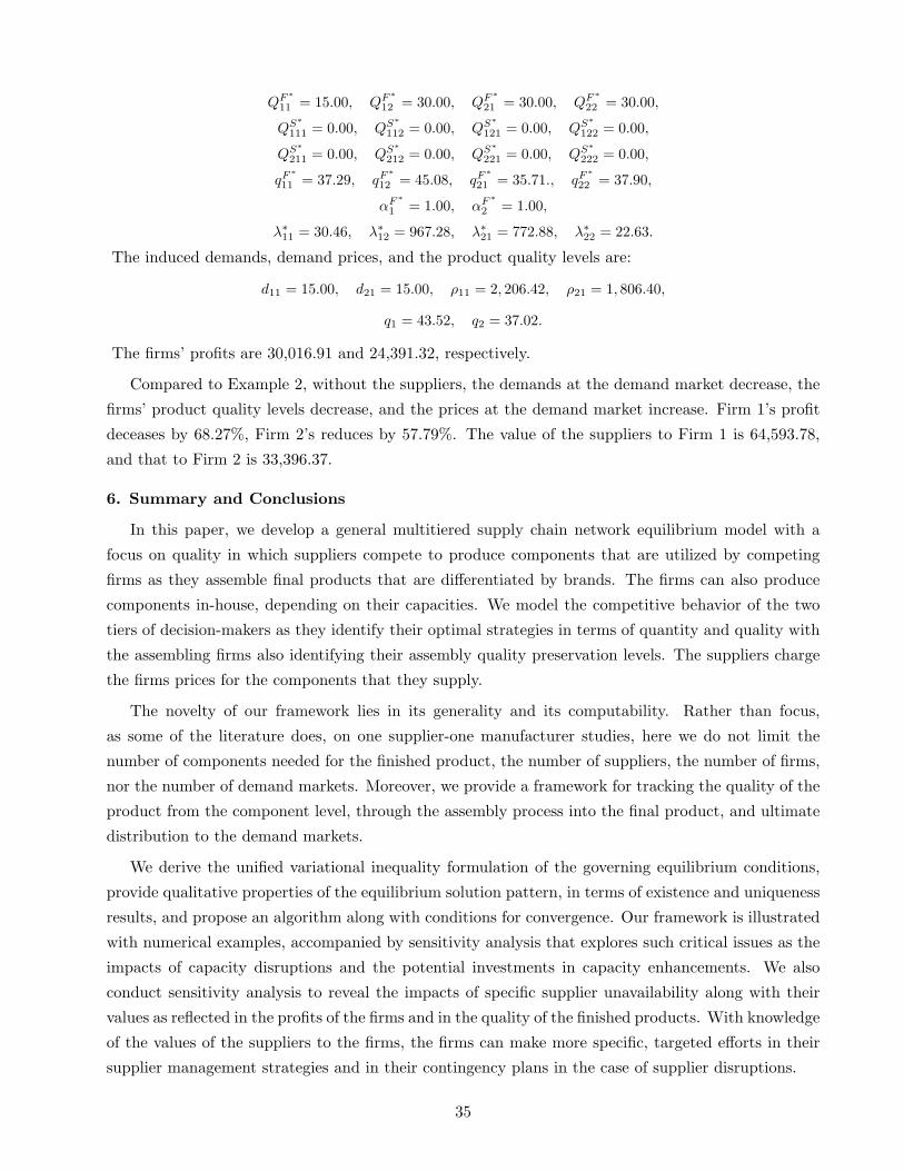
QF∗
11 = 15.00, QF∗
12 = 30.00, QF∗
21 = 30.00, QF∗
22 = 30.00,
QS∗
111 = 0.00, QS∗
112 = 0.00, QS∗
121 = 0.00, QS∗
122 = 0.00,
QS∗
211 = 0.00, QS∗
212 = 0.00, QS∗
221 = 0.00, QS∗
222 = 0.00,
qF∗
11 = 37.29, qF∗
12 = 45.08, qF∗
21 = 35.71., qF∗
22 = 37.90,
αF∗
1 = 1.00, αF∗
2 = 1.00,
λ∗11 = 30.46, λ∗12 = 967.28, λ∗21 = 772.88, λ∗22 = 22.63.
The induced demands, demand prices, and the product quality levels are:
d11 = 15.00, d21 = 15.00, ρ11 = 2, 206.42, ρ21 = 1, 806.40,
q1 = 43.52, q2 = 37.02.
The firms’ profits are 30,016.91 and 24,391.32, respectively.
Compared to Example 2, without the suppliers, the demands at the demand market decrease, the
firms’ product quality levels decrease, and the prices at the demand market increase. Firm 1’s profit
deceases by 68.27%, Firm 2’s reduces by 57.79%. The value of the suppliers to Firm 1 is 64,593.78,
and that to Firm 2 is 33,396.37.
6. Summary and Conclusions
In this paper, we develop a general multitiered supply chain network equilibrium model with a
focus on quality in which suppliers compete to produce components that are utilized by competing
firms as they assemble final products that are differentiated by brands. The firms can also produce
components in-house, depending on their capacities. We model the competitive behavior of the two
tiers of decision-makers as they identify their optimal strategies in terms of quantity and quality with
the assembling firms also identifying their assembly quality preservation levels. The suppliers charge
the firms prices for the components that they supply.
The novelty of our framework lies in its generality and its computability. Rather than focus,
as some of the literature does, on one supplier-one manufacturer studies, here we do not limit the
number of components needed for the finished product, the number of suppliers, the number of firms,
nor the number of demand markets. Moreover, we provide a framework for tracking the quality of the
product from the component level, through the assembly process into the final product, and ultimate
distribution to the demand markets.
We derive the unified variational inequality formulation of the governing equilibrium conditions,
provide qualitative properties of the equilibrium solution pattern, in terms of existence and uniqueness
results, and propose an algorithm along with conditions for convergence. Our framework is illustrated
with numerical examples, accompanied by sensitivity analysis that explores such critical issues as the
impacts of capacity disruptions and the potential investments in capacity enhancements. We also
conduct sensitivity analysis to reveal the impacts of specific supplier unavailability along with their
values as reflected in the profits of the firms and in the quality of the finished products. With knowledge
of the values of the suppliers to the firms, the firms can make more specific, targeted efforts in their
supplier management strategies and in their contingency plans in the case of supplier disruptions.
35

Future research may include the solution of larger numerical examples as well as the computational
exploration of enhancements to the algorithmic scheme (see, for example, Fu and He (2010) and He,
Yuan, and Zhang (2004)). .
Acknowledgments
We sincerely thank the three anonymous referees for their many valuable suggestions and comments.
This research was supported, in part, by the National Science Foundation (NSF) grant CISE #1111276,
for the NeTS: Large: Collaborative Research: Network Innovation Through Choice project awarded
to the University of Massachusetts Amherst. This support is gratefully acknowledged.
References
Acharyya, R., 2005. Consumer targeting under quality competition in a liberalized vertically differ-
entiated market. Journal of Economic Development, 30(1), 129-150.
Akerlof, G.A., 1970. The market for ‘lemons’: Quality uncertainty and the market mechanism. Quar-
terly Journal of Economics, 84(3), 488-500.
Amaral, J., Billington, C., Tsay, A., 2006. Safeguarding the promise of production outsourcing.
Interfaces, 36(3), 220-233.
Aoki, R., Prusa, T.J., 1997. Sequential versus simultaneous choice with endogenous quality. Interna-
tional Journal of Industrial Organization, 15(1), 103-121.
Bailey, B., 2007. Where does your food come from? Food labels don’t tell the whole inside story.
Mercury News, July 22.
Baiman, S., Fischer, P.E., Rajan, M.V., 2000. Information, contracting, and quality costs. Manage-
ment Science, 46(6), 776-789.
Banker, R.D., Khosla, I., Sinha, K.K., 1998. Quality and competition. Management Science, 44(9),
1179-1192.
Bender, P.S., Brown, R.W., Isaac, M.H., Shapiro, J.F., 1985. Improving purchasing productivity at
IBM with a normative decision support system. Interfaces, 15(3), 106-115.
Bertrand, J., 1883. Theorie mathematique de la richesse sociale. Journal des Savants, September,
499-508.
Bertsekas, D.P., Tsitsiklis, J.N., 1989. Parallel and distributed computation - Numerical methods.
Prentice Hall, Englewood Cliffs, New Jersey.
Bomey, N., 2014. Maker of GM ignition switches stymies investigation. USA Today, June 22.
Brekke, K.R., Siciliani, L., Straume, O.R., 2010. Price and quality in spatial competition. Regional
Science and Urban Economics, 40(6), 471-480.
36

Buzzell, R.D., Gale, B.T., 1987. The PIMS principles: Linking strategy to performance. Free Press,
New York.
Campanella, J., 1990. Principles of quality costs, second edition. ASQC Quality Press, Milwaukee,
Wisconsin.
Chambers, C., Kouvelis, P., Semple, J., 2006. Quality-based competition, profitability, and variable
costs. Management Science, 52(12), 1884-1895.
Chan, Y.S., Leland, H.E., 1982. Prices and qualities in markets with costly information. The Review
of Economic Studies, 49(4), 499-516.
Chao, G.H., Iravani, S.M., Savaskan, R.C., 2009. Quality improvement incentives and product recall
cost sharing contracts. Management Science, 55(7), 1122-1138.
Cheng, T.C.E., 1991. EPQ with process capability and quality assurance considerations. Journal of
the Operational Research Society, 42(8), 713-720.
Cournot, A.A., 1838. Researches into the mathematical principles of the theory of wealth, English
translation. MacMillan, London, England.
Crosby, P.B., 1979. Quality is free. McGraw-Hill, New York.
Deming, W.E., 1986. Out of the crisis. Massachusetts Institute of Technology Center for Advanced
Engineering Study, Cambridge, Massachusetts.
Denning, S., 2013. What went wrong with Boeing? Forbes, January 21.
Dixit, A., 1979. Quality and quantity competition. Review of Economic Studies, 46(4), 587-599.
Drew, C., 2014. Suppliers of jet parts require greater oversight, report says. The New York Times,
March 19.
Economides, N., 1999. Quality choice and vertical integration. International Journal of Industrial
Organization, 17(6), 903-914.
El Ouardighi, F., Kim, B., 2010. Supply quality management with wholesale price and revenue-sharing
contracts under horizontal competition. European Journal of Operational Research, 206(2), 329-340.
El Ouardighi, F., Kogan, K., 2013. Dynamic conformance and design quality in a supply chain: an
assessment of contracts? coordinating power. Annals of Operations Research, 211(1), 137-166.
Feigenbaum, A.V., 1982. Quality and business growth today. Quality progress, 15(11), 22-25.
Feigenbaum, A.V., 1983. Quality costs in total quality control, third edition. McGraw-Hill, New York.
Foster, S.T. Jr., 2008. Towards an understanding of supply chain quality management. Journal of
Operations Management, 26(4), 461-467.
Fu, X., He, B., 2010. Self-adaptive projection-based prediction-correction method for constrained
variational inequalities. Frontiers of Mathematics in China, 5(1), 3-21.
37

Gabay, D., Moulin, H., 1980. On the uniqueness and stability of Nash equilibria in noncooperative
games. In: Bensoussan, A., Kleindorfer, P., Tapiero, C.S. (Eds.). Applied stochastic control in
econometrics and management science, 271-294. North-Holland, Amsterdam, The Netherlands.
Gal-Or, E., 1983. Quality and quantity competition. Bell Journal of Economics, 14(2), 590-600.
Ghodsypour, S.H., O’Brien, C., 2001. The total cost of logistics in supplier selection, under conditions
of multiple sourcing, multiple criteria and capacity constraint. International journal of production
economics, 73(1), 15-27.
Gilmore, H.L., 1974. Product conformance cost. Quality Progress, 7(5), 16-19.
Harris, G., 2009. Peanut plant broadens product list under recall. The New York Times, January 29.
He, B.S., Yuan, X.M., Zhang, J.J.Z., 2004. Comparison of two kinds of prediction-correction methods
for monotone variational inequalities. Computational Optimization and Applications, 27, 247-267.
Hong, J.D., Hayya, J.C., 1992. Just-in-time purchasing: Single or multiple sourcing? International
Journal of Production Economics, 27(2), 175-181.
Hotelling, H., 1929. Stability in competition. The Economic Journal, 39(153), 41-57.
Hsieh, C.C., Liu, Y.T., 2010. Quality investment and inspection policy in a suppliermanufacturer
supply chain. European Journal of Operational Research, 202(3), 717-729.
Hwang, I., Radhakrishnan, S., Su, L.N., 2006. Vendor certification and appraisal: Implications for
supplier quality. Management Science, 52(10), 1472-1482.
Jayaraman, V., Srivastava, R., Benton, W.C., 1999. Supplier selection and order quantity allocation:
A comprehensive model. Journal of Supply Chain Management, 35(1), 50-58.
Juran, J.M., 1951. Quality control handbook. McGraw-Hill, New York.
Juran, J.M., Gryna, F.M., 1988. Quality control handbook, fourth edition. McGraw-Hill, New York.
Kageyama, Y., 2011. Thai floods: Honda under water. The World Post, November 10.
Kinderlehrer, D., Stampacchia, G., 1980. An introduction to variational inequalities and their appli-
cations. Academic Press, New York.
Korpelevich, G.M., 1977. The extragradient method for finding saddle points and other problems.
Matekon, 13, 35-49.
Kubota, Y., Klayman, B., 2013. Japan carmakers recall 3.4 million vehicles for Takata airbag flaw.
Reuter, April 11.
Lederer, P.J., Rhee, S.K., 1995. Economics of total quality management. Journal of Operations
Management, 12(3), 353-367.
Lehmann-Grube, U., 1997. Strategic choice of quality when quality is costly: The persistence of the
high quality advantage. RAND Journal of Economics, 28(3), 372-384.
38

Leland, H.E., 1977. Quality choice and competition. American Economics Review, 67(2), 127-137.
Leland, H.E., 1979. Quacks, lemons, and licensing: A theory of minimum quality standards. Journal
of Political Economy, 87(6), 1328-1346.
Levitt, T., 1972. Production-line approach to service. Harvard Business Review, 50(5), 41-52.
Lim, W.S., 2001. Producer-supplier contracts with incomplete information. Management Science,
47(5), 709-715.
Liu, Z., Nagurney, A., 2009. An integrated electric power supply chain and fuel market network
framework: Theoretical modeling with empirical analysis for New England. Naval Research Logistics,
56, 600-624.
Lohr, S., 2011. Stress test for the global supply chain. The New York Times, March 19.
Lu, Y., Ng, T., Tao, Z., 2012. Outsourcing, product quality, and contract enforcement. Journal of
Economics & Management Strategy, 21(1), 1-30.
Marucheck, A., Greis, N., Mena, C., Cai, L., 2011. Product safety and security in the global supply
chain: Issues, challenges and research opportunities. Journal of Operations Management, 29(7), 707-
720.
Masoumi, A.H., Yu, M., Nagurney, A., 2012. A supply chain generalized network oligopoly model
for pharmaceuticals under brand differentiation and perishability. Transportation Research E, 48,
762-780.
McDonald, J., 2014. Meat scandal hits China Starbucks, Burger King. Masslive, July 22.
Motta, M., 1993. Endogenous quality choice: Price vs. quantity competition. The Journal of Indus-
trial Economics, 41(2), 113-131.
Nagurney, A., 1999. Network economics: A variational inequality approach. Kluwer Academic Pub-
lishers, Dordrecht, The Netherlands.
Nagurney, A., 2006. Supply chain network economics: Dynamics of prices, flows, and profits. Edward
Elgar Publishing, Cheltenham, England.
Nagurney, A., Dhanda, K.K., 2000. Marketable pollution permits in oligopolistic markets with trans-
action costs. Operations Research, 48(3), 424-435.
Nagurney, A., Li, D., 2014a. Equilibria and dynamics of supply chain network competition with infor-
mation asymmetry in quality and minimum quality standards. Computational Management Science,
11(3), 285-315.
Nagurney, A., Li, D., 2014b. A dynamic network oligopoly model with transportation costs, product
differentiation, and quality competition. Computational Economics, 44(2), 201-229.
Nagurney, A., Li, D., 2015. A supply chain network game theory model with product differentiation,
39

outsourcing of production and distribution, and quality and price competition, Annals of Operations
Research, 228(1), 479-503.
Nagurney, A., Li, D., Nagurney, L.S., 2013. Pharmaceutical supply chain networks with outsourcing
under price and quality competition. International Transactions in Operational Research, 20(6), 859-
888.
Nagurney, A., Li. D., Nagurney, L.S., 2014. Spatial price equilibrium with information asymmetry in
quality and minimum quality standards. International Journal of Production Economics, 158, 300-313.
Nagurney, A., Li, D., Wolf, T., Saberi, S., 2013a. A network economic game theory model of a
service-oriented Internet with choices and quality competition. Netnomics, 14(1-2), 1-25.
Nagurney, A., Li, D., Saberi S., Wolf, T., 2014. A dynamic network economic model of a service-
oriented Internet with price and quality competition. In: Kalyagin, V.A., Pardalos, P.M., Rassias,
T.M. (Eds.). Network models in economics and finance. Springer International Publishing Switzerland,
239-264
Nagurney, A., Masoumi, A.H., 2012. Supply chain network design of a sustainable blood banking
system. In: Boone, T., Jayaraman, V., Ganeshan, R. (Eds.). Sustainable supply chains: Models,
methods and public policy implications. Springer, London, England, 49-72.
Nagurney, A., Nagurney, L., 2012. Medical nuclear supply chain design: A tractable network model
and computational approach. International Journal of Production Economics, 140(2), 865-874.
Nagurney, A., Yu, M., Masoumi, A.H., Nagurney, L.S., 2013b. Networks against time: Supply chain
analytics for perishable products. Springer Business + Science Media, New York.
Nash, J.F., 1950. Equilibrium points in n-person games. Proceedings of the National Academy of
Sciences, USA 36, 48-49.
Nash, J.F., 1951. Noncooperative games. Annals of Mathematics, 54, 286-298.
Oliver, R. L., 1981. Measurement and evaluation of satisfaction processes in retail settings. Journal
of Retailing, 57(3), 25-48.
Parker, A., 2014. Boeing hit by fresh 787 battery problem. Financial Times, January 14.
Pennerstorfer, D., Weiss, C.R., 2012. Product quality in the agri-food chain: Do cooperatives offer
high-quality wine? European Review of Agricultural Economics, 40(1), 143-162.
Porter, L.J., Rayner, P., 1992. Quality costing for total quality management. International Journal
of Production Economics, 27(1), 69-81.
Porteus, E.L., 1986. Optimal lot sizing, process quality improvement and setup cost reduction. Op-
erations research, 34(1), 137-144.
Rao, R., 2014. Indian bulk drug industry: Maintain quality conscience to face competition. Business
Standards, January 16.
40

Reyniers, D.J., Tapiero, C.S., 1995. The delivery and control of quality in supplier-producer contracts.
Management Science, 41(10), 1581-1589.
Rezaei, J., Davoodi, M., 2008. A deterministic, multi-item inventory model with supplier selection
and imperfect quality. Applied Mathematical Modelling, 32(10), 2106-2116.
Robinson, C.J., Malhotra, M.K., 2005. Defining the concept of supply chain quality management and
its relevance to academic and industrial practice. International Journal of Production Economics,
96(3), 315-337.
Rosenthal, E.C., Zydiak, J.L., Chaudhry, S.S., 1995. Vendor selection with bundling. Decision Sci-
ences, 26(1), 35-48.
Seetharaman, D., 2013. Surge in auto production impairs quality of parts, Ford purchasing boss says.
Automotive News, October 21.
Shaked, A., Sutton, J., 1982. Relaxing price competition through product dfferentiation. The Review
of Economic Studies, 49(1), 3-13.
Shank, J.K., Govindarajan, V., 1994. Measuring the cost of quality: A strategic cost management
perspective. Journal of Cost Management, 8(2), 5-17.
Shewhart, W.A., 1931. Economic control of quality of manufactured product. Van Nostrand, New
York.
Shi, H., Liu, Y., Petruzzi, N.C., 2013. Consumer heterogeneity, product quality, and distribution
channels. Management Science, 59(5), 1162-1176.
Starbird, S.A., 1997. Acceptance sampling, imperfect production, and the optimality of zero defects.
Naval Research Logistics, 44(6), 515-530.
Story, L., Barboza, D., 2007. Mattel recalls 19 million toys sent from China. The New York Times,
August 15.
Stout, H., Ivory, D., Wald, M.L., 2014. Auto regulators dismissed defect tied to 13 deaths. The New
York Times, March 8.
Strom, S., 2013. Taylor farms, big food supplier, grapples with frequent recalls. The New York Times,
August 19.
Tabuchi, H., Jensen, C., 2014. Now the air bags are faulty too - Takata acknowledges poor records in
air bag recall. The New York Times, June 23.
Tagaras, G., Lee, H.L., 1996. Economic models for vendor evaluation with quality cost analysis.
Management Science, 42(11), 1531-1543.
Tang, C.S., 2008. Making products safe: Process and challenges. International Commerce Review, 8,
48-55.
41

Xie, G., Yue, W., Wang, S., Lai, K.K., 2011. Quality investment and price decision in a risk-averse
supply chain. European Journal of Operational Research, 214(2), 403-410.
Xu, X., 2009. Optimal price and product quality decisions in a distribution channel. Management
Science, 55(8), 1347-1352.
Yip, G.S., 1989. Global strategy in a world of nations. Sloan Management Review, 89(1), 29-41.
Yu, M., Nagurney, A., 2013. Competitive food supply chain networks with application to fresh produce.
European Journal of Operational Research, 224(2), 273-282.
Zhu, K., Zhang, R.Q., Tsung, F., 2007. Pushing quality improvement along supply chains. Manage-
ment science, 53(3), 421-436.
42

Appendix
Proof of Theorem 1:
For a given firm i, under the imposed assumptions, (16) holds if and only if (see Bertsekas and
Tsitsiklis (1989) page 287) the following holds:
nR∑k=1
[−∂UF
i (Q∗, QF ∗, QS∗, qF∗, αF∗
, π∗i , qS∗)
∂Qik+
nli∑l=1
λ∗ilθil
]× (Qik −Q∗
ik)
+nli∑l=1
[−∂UF
i (Q∗, QF ∗, QS∗, qF∗, αF∗
, π∗i , qS∗)
∂QFil
− λ∗il
]× (QF
il −QF∗
il )
+nS∑j=1
nli∑l=1
[−∂UF
i (Q∗, QF ∗, QS∗, qF∗, αF∗
, π∗i , qS∗)
∂QSjil
− λ∗il
]× (QS
jil −QS∗
jil)
+nli∑l=1
[−∂UF
i (Q∗, QF ∗, QS∗, qF∗, αF∗
, π∗i , qS∗)
∂qFil
]× (qF
il − qF∗
il )
+
[−∂UF
i (Q∗, QF ∗, QS∗, qF∗, αF∗
, π∗i , qS∗)
∂αFi
]× (αF
i − αF∗
i )
+nli∑l=1
nS∑j=1
QS∗
jil + QF∗
il −nR∑k=1
Q∗ikθil
× (λil − λ∗il) ≥ 0, ∀(Qi, QFi , QS
i , qFi , αF
i , λi) ∈ KFi . (A1)
Variational inequality (A1) holds for each firm i; i = 1, . . . , I, and, hence, the summation of (A1)
yields variational inequality (17).�
Proof of Theorem 4:
We first prove that there exists at least one solution to variational inequality (26) (cf. (22)). Note
that, all the component quality levels, qSjil and qF
il , and quality preservation levels αi are bounded
due to constraints (3), (4), and (7). Because of constraint (12), all the product quantities Qik are
also bounded, since the components quantities are nonnegative and capacitated (cf. (13) and (14)).
Therefore, with Assumption 1, the feasible set of variational inequality (26) is bounded. Since the
cost functions and the demand price functions are continuously differentiable, and the feasible set is
convex and compact, the existence of a solution to (26) (cf. (22)) is guaranteed (cf. Kinderlehrer
and Stampacchia (1980) and Theorem 1.5 in Nagurney (1999)). Because (26) and (24) (cf. (23)) are
equivalent (Nagurney and Dhanda (2000)), the existence of (24) is also guaranteed. �
Proof of Theorem 5:Let Y ′ = (Q′, QS′
, QF ′, qF ′
, αF ′, π′, qS′
), Y ′′ = (Q′′, QS′′, QF ′′
, qF ′′, αF ′′
, π′′, qS′′), X ′ = (Q′, QS′
, QF ′,
qF ′, αF ′
, λ′, π′, qS′), and X ′′ = (Q′′, QS′′
, QF ′′, qF ′′
, αF ′′, λ′′, π′′, qS′′
). Then the left-hand-side of (29)can be expended to:
IXi=1
nRXk=1
"(−
∂UFi (Q′, QS′
, QF ′, qF ′
, αF ′, π′, qS′
)
∂Qik)− (−
∂UFi (Q′′, QS′′
, QF ′′, qF ′′
, αF ′′, π′′, qS′′
)
∂Qik)
#× (Q′
ik − Q′′ik)
+IX
i=1
nliX
l=1
"(−
∂UFi (Q′, QS′
, QF ′, qF ′
, αF ′, π′, qS′
)
∂QFil
)− (−∂UF
i (Q′′, QS′′, QF ′′
, qF ′′, αF ′′
, π′′, qS′′)
∂QFil
)
#× (QF ′
il − QF ′′il )
43
+
nSXj=1
IXi=1
nliX
l=1
"(−
∂UFi (Q′, QS′
, QF ′, qF ′
, αF ′, π′, qS′
)
∂QSjil
)− (−∂UF
i (Q′′, QS′′, QF ′′
, qF ′′, αF ′′
, π′′, qS′′)
∂QSjil
)
#× (QS′
jil − QS′′jil )
+IX
i=1
nliX
l=1
"(−
∂UFi (Q′, QS′
, QF ′, qF ′
, αF ′, π′, qS′
)
∂qFil
)− (−∂UF
i (Q′′, QS′′, QF ′′
, qF ′′, αF ′′
, π′′, qS′′)
∂qFil
)
#× (qF ′
il − qF ′′il )
+IX
i=1
"(−
∂UFi (Q′, QS′
, QF ′, qF ′
, αF ′, π′, qS′
)
∂αFi
)− (−∂UF
i (Q′′, QS′′, QF ′′
, qF ′′, αF ′′
, π′′, qS′′)
∂αFi
)
#× (αF ′
i − αF ′′i )
+
nSXj=1
IXi=1
nliX
l=1
"(−
∂USj (QS′
, π′, qS′)
∂πjil)− (−
∂USj (QS′′
, π′′, qS′′)
∂πjil)
#× (π′
jil − π′′jil)
+
nSXj=1
IXi=1
nliX
l=1
"(−
∂USj (QS′
, π′, qS′)
∂qSjil
)− (−∂US
j (QS′′, π′′, q′′)
∂qSjil
)
#× (qS′
jil − qS′′jil )
+IX
i=1
nRXk=1
24nliX
l=1
λ′ilθil −
nliX
l=1
λ′ilθil
35 × (Q′ik − Q′′
ik) +IX
i=1
nRXk=1
24nliX
l=1
λ′′ilθil −
nliX
l=1
λ′′ilθil
35 × (Q′ik − Q′′
ik)
+IX
i=1
nliX
l=1
ˆλ′
il − λ′il
˜× (QF ′
il − QF ′′il ) +
IXi=1
nliX
l=1
ˆλ′′
il − λ′′il
˜× (QF ′
il − QF ′′il )
+
nSXj=1
IXi=1
nliX
l=1
ˆλ′
il − λ′il
˜× (QS′
jil − QS′′jil ) +
nSXj=1
IXi=1
nliX
l=1
ˆλ′′
il − λ′′il
˜× (QS′
jil − QS′′jil ). (A2)
where λ′il, λ′′il ≥ 0, i = 1, . . . , I, l = 1, . . . , nli .
After combining terms, (A2) reduces toIX
i=1
nRXk=1
24(−∂UF
i (Q′, QS′, QF ′
, qF ′, αF ′
, π′, qS′)
∂Qik+
nliX
l=1
λ′ilθil)− (−
∂UFi (Q′′, QS′′
, QF ′′, qF ′′
, αF ′′, π′′, qS′′
)
∂Qik+
nliX
l=1
λ′′ilθil)
35×(Q′
ik − Q′′ik)
+IX
i=1
nliX
l=1
"(−
∂UFi (Q′, QS′
, QF ′, qF ′
, αF ′, π′, qS′
)
∂QFil
− λ′il)− (−
∂UFi (Q′′, QS′′
, QF ′′, qF ′′
, αF ′′, π′′, qS′′
)
∂QFil
− λ′′il)
#× (QF ′
il − QF ′′il )
+
nSXj=1
IXi=1
nliX
l=1
"(−
∂UFi (Q′, QS′
, QF ′, qF ′
, αF ′, π′, qS′
)
∂QSjil
− λ′il)− (−
∂UFi (Q′′, QS′′
, QF ′′, qF ′′
, αF ′′, π′′, qS′′
)
∂QSjil
− λ′′il)
#× (QS′
jil −QS′′jil )
+IX
i=1
nliX
l=1
"(−
∂UFi (Q′, QS′
, QF ′, qF ′
, αF ′, π′, qS′
)
∂qFil
)− (−∂UF
i (Q′′, QS′′, QF ′′
, qF ′′, αF ′′
, π′′, qS′′)
∂qFil
)
#× (qF ′
il − qF ′′il )
+IX
i=1
"(−
∂UFi (Q′, QS′
, QF ′, qF ′
, αF ′, π′, qS′
)
∂αFi
)− (−∂UF
i (Q′′, QS′′, QF ′′
, qF ′′, αF ′′
, π′′, qS′′)
∂αFi
)
#× (αF ′
i − αF ′′i )
+
nSXj=1
IXi=1
nliX
l=1
"(−
∂USj (QS′
, π′, qS′)
∂πjil)− (−
∂USj (QS′′
, π′′, qS′′)
∂πjil)
#× (π′
jil − π′′jil)
+
nSXj=1
IXi=1
nliX
l=1
"(−
∂USj (QS′
, π′, qS′)
∂qSjil
)− (−∂US
j (QS′′, π′′, q′′)
∂qSjil
)
#× (qS′
jil − qS′′jil )
+IX
i=1
nliX
l=1
24(
nSXj=1
QS′jil + QF ′
il −nRXk=1
Q′ikθil)− (
nSXj=1
QS′′jil + QF ′′
il −nRXk=1
Q′′ikθil)
35 × (λ′il − λ′′
il). (A3)
The expression in (A2), equivalently, (A3), is greater than or equal to zero, since we have assumed
in Theorems 1 and 2 that the profit functions are concave with respect to associated variables. (A2) is
derived from the left-hand-side of (29), so (29) holds true, and, hence, the G(Y ) that enters variational
inequality (26) is monotone. Because (A3) is also the left-hand-side of (28), the F (X) that enters
variational inequality (24) is also monotone. �
44
Top Related